Lab #5 DDL (Direct Differential Leveling)bechtel.colorado.edu/~halek/Spring_2016_Field_Book.docx ·...

CVEN 2012 Name:________________Group #:______________

FIELD BOOK

(Lab Manual Spring 2016)

Lab # Date: Signature: TOPIC:

1

2

3

4

5

6

7

8

9

10

11

Sr. Instructor: Milan Halek Website: http://bechtel.colorado.edu/~halek/index

Lab #1: Introduction

Objectives:

1. Create a freehand topographical sketch of your group’s plot of land.

2. Practice converting angles from decimal degrees to DMS (Degrees Minutes Seconds), and back

by hand and with the calculator.

Equipment:

Field book, pencil, and calculator

Lab Procedure:

Topographical Sketch

Create a sketch of your plot of land on the data page below.

Angles

By Hand:

DMS to decimal:

5 °6 ' 7 =5+ { {6+ { {7} over { 60 } } } over {60 } } =5 . 1019 °} {¿Decimal to DMS:

5 .1019 °=5 ° (0 .1019⋅60) '=5° 6 . 114 '=5 °6 ' (0 .114⋅60)=5°6'7

With your calculator (TI 83/84 and 89 shown here):

1. Press the ‘Mode’ key, and verify that angles are set to degrees, and NOT radians.

2. It is simple to work with angles on TI calculators. Simply type in the examples like the ones

shown below. The difficult part is finding the , ‘, “, and ¿ DMS symbols.

- For the TI83/84, the “ symbol is just above the + key. The ‘ ¿ DMS symbols are

found under the Second Angle menu.

- For the TI89, the ‘ “ symbols are found on the keypad, and the ¿ DMS symbol is

found under the Second Math menu.

3. Practice the conversions shown below.

Input: 56’7”

Output: 5.10194

Input: 5.1019444 > DMS

Output: 56’7”

Input: (23°3 ' 45+32 °43 ' 12 )>DMS

Output: 5546’57”

Input: 359 °52 ' 32. 3 \( 21 . 568222 / 24 \) + 180°37 ' 25 . 5−360 °>DMS

Output: 1442’7.2”


Note Page

Name: ________________________

Phone: ________________________

E-mail: ________________________

Crew #: ________________________

Crew Members: ________________________

________________________

________________________

________________________

________________________

Weather: ____________________________

Equipment: ________________________________________________

________________________________________________

Notes: ________________________________________________

________________________________________________

________________________________________________

________________________________________________

________________________________________________

________________________________________________

________________________________________________

________________________________________________

________________________________________________


Data Page - Topographical Sketch (Free-hand)

LeveledUnleveled

Lab #2: Interior Angle Measurement

Objectives:

3. Practice theodolite setup (Centering, Leveling)

4. Measure angle twice at direct and reversed position. Repeat the process for each of three points.

5. Practice computing adjusted angles from measured data.

Equipment:

Theodolite, Tripod, Rod, Plumb bob, and Field Book

Lab Procedure

Centering

Our theodolites have two types of centering features. One is an optical plumb bob, and the other is a

laser plumb bob. A little scope is located at the lower part of the theodolite. Through the scope, locate

the rebar or point of beginning. Some of the theodolites are equipped with a laser plumb bob, in this

case, locate the laser right on the center of the rebar.

Approximate leveling

Level the instrument with the adjustable legs of the tripod. Do

your best to bring the air bubble as close as possible to center

mark. Adjusting the length of the tripod legs, without moving

them, does not change the location of the point that the optical

plum bob or laser is pointed at.

Fine tune leveling

Leveling with leveling screws changes the location of the point

that the optical plum bob or laser is pointed at. Therefore, use it only for fine tune. A circular level

bubble can be found on one side of the scope. Operate three leveling screws to locate the bubble to the

center of the circular window. Three leveling screws are located at the bottom of the scope. Turning

each screw, raise or lower one side of the plate. Starting with any two three screws, rotate them

simultaneously inward or outward as the picture on the left

shows. Turning two screws simultaneously clockwise or

counterclockwise won’t do anything.


Angle Measurement

Measuring Interior Angle at each of your three points

1. Setup the equipment at one of your point (center and level the equipment)

2. Take a Direct Reading and record.

3. Plunge the scope

4. Take a Reverse Reading and record

5. Repeat the process for other two points

Recording the DataT @ A, CW Direct Reverse MeanB 0°00’00” 180°00’00”C 60°00’00” 240°02’20”Interior Angle 60°00’00” 60°02’20” 60°01’10”

Angle AdjustmentStation Measured AdjustedA 60°01’10” 60°00’50”B 60°00’00” 59°59’40”C 59°59’50” 59°59’30”

Sum = 60°01’10” + 60°00’00” + 59°59’50” = 180°01’00”

Misclosure: + 0°01’00”

Adjustment: - 0°01’00” / 3 = - 0°00’20”


Note Page

Name: ________________________

Crew: ________________________

Date: ________________________

Weather: ________________________

Equipment: ________________________________________________

________________________________________________

Notes: ________________________________________________

________________________________________________

________________________________________________

________________________________________________

________________________________________________

________________________________________________

________________________________________________

________________________________________________

________________________________________________

Sketch:


Data Page

STA @___ Direct Reverse

Sighting To:____

Sighting To:____ Mean

Interior Angle


Sighting To:____


Interior Angle


Sighting To:____


Interior Angle


Sighting To:____


Interior Angle

Station Measured + Correction = AdjustedABC

SUM

Misclosure = Correction =

Feb 1 -17° 16’ 42.6” 176° 37’ 53.3” 0° 16’ 13.9”Feb 2 -16° 59’ 40.5” 176° 35’ 48.8” 0° 16’ 13.8”

Theodolite @ __A_Sighting To Telescope Time ReadingPoint __B_ Direct ---------------------- 0° 00’ 00”

Sun Direct 1:46:10 PM 204° 00’ 40”Sun Direct 1:46:56 PM 204° 10’ 54”Sun Reversed 1:49:05 PM 25° 40’ 24”Sun Reversed 1:49:52 PM 25° 50’ 42”

Point_B__ (same as above) Reversed ---------------------- 180° 00’ 41”

Wolfpack input file:Lab Manual Example File Title39 58 23.9 105 11 44.9 Observer’s latitude and longitude176 37 53.3 176 35 48.8 GHA at 0 and 24 Hours-17 16 42.6 -16 59 40.5 0 16 13.85 1 Declination at 0 and 24 Hours, Semi-Diameter7 0 0 0 Time correction (7 hrs for MST and 6 for MDT)1 13 46 10 0 0 0 204 00 40 First reading ( #, Time, BS Angle, Horiz. Angle)2 13 46 56 0 0 0 204 10 54 Second reading3 13 49 05 180 0 41 25 40 24 Third reading4 13 49 52 180 0 41 25 50 42 Fourth reading

Sun

BC

A

Sun

Sun

Output data:----------------------------------------

Lab Manual Example

Observer's Astronomic Position: Latitude = 39°58'23.9" Longitude = 105°11'44.9"

Semi-diamter at 0h UT : 0°16'13.8" sighting trailing edge.

StopWatch Start Time, UTC: 7:00:00.0 DUT correction: 0.0sec

GHA of Sun at 0h UT : 176°37'53.30"GHA of Sun at 24h UT : 176°35'48.80"

Declination of Sun at 0h UT : -17°16'42.60"Declination of Sun at 24h UT : -16°59'40.50"

Pointing Time Hor. Angle Declination L H A Azimuth to Star Az of Line------------------------------------------------------------------------------------------------------------------- 1 20:46:10.0 204°00'40" -17°01'59.09" 22°56'50.7" 205°15'30" 0°56'15" 2 20:46:56.0 204°10'54" -17°01'58.54" 23°08'20.6" 205°27'19" 0°57'51" 3 20:49:05.0 205°39'43" -17°01'57.01" 23°40'35.4" 206°00'22" 0°02'07" 4 20:49:52.0 205°50'01" -17°01'56.45" 23°52'20.3" 206°12'22" 0°03'49"------------------------------------------------------------------------------------------------------------------- Average Astronomic Azimuth of Line = 0°30'00.4" Deviation in the mean = 937.1"

- Sun shots corrected for leading/trailing edges.

Some notes about using Wolfpack software to complete solar calculations:

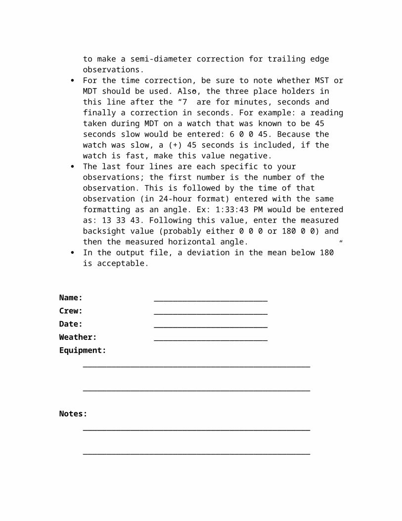
The file must have a title. If it does not, the input will be misread and results will be incorrect.

For every entry involving an angle, input data in DMS (degree, minute, second) format. Ex: 180 23’ 45” would be entered 180 23 45. The only formatting required is a space between each value.

In the third line of input data, be sure to include a “1” at the very end of the line. This tells the program to make a semi-diameter correction for trailing edge observations.

For the time correction, be sure to note whether MST or MDT should be used. Also, the three place holders in this line after the “7” are for minutes, seconds and finally a correction in seconds. For example: a reading taken during MDT on a watch that was known to be 45 seconds slow would be entered: 6 0 0 45. Because the watch was slow, a (+) 45 seconds is included, if the watch is fast, make this value negative.

The last four lines are each specific to your observations; the first number is the number of the observation. This is followed by the time of that observation (in 24-hour format) entered with the same formatting as an angle. Ex: 1:33:43 PM would be entered as: 13 33 43. Following this value, enter the measured backsight value (probably either 0 0 0 or 180 0 0) and then the measured horizontal angle.

In the output file, a deviation in the mean below 180” is acceptable.

Name: ________________________

Crew: ________________________

Date: ________________________

Weather: ________________________

Equipment: ________________________________________________

________________________________________________

Notes: ________________________________________________

________________________________________________

________________________________________________

________________________________________________

________________________________________________

________________________________________________

________________________________________________

________________________________________________________________________________________________

Sketch:

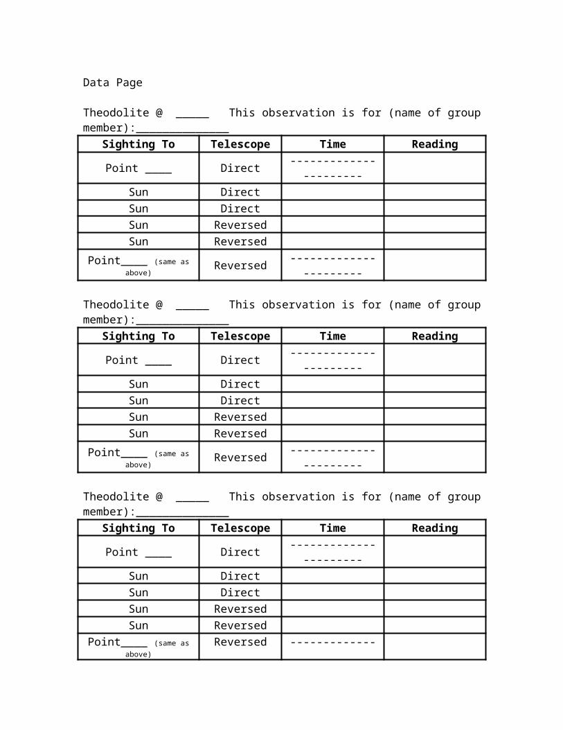
Data Page

Theodolite @ _____ This observation is for (name of group member):______________Sighting To Telescope Time ReadingPoint ____ Direct ----------------------

Sun DirectSun DirectSun ReversedSun Reversed

Point____ (same as above) Reversed ----------------------










Lab #3: Distances

Objectives:

1. Find distance of your four property lines

2. Familiarize yourself with the functions of total station

3. Practice manual distance measurement using measuring tape

Equipment:

Total Station, Tripod, Pin, Plumb bob, reflection rod, and Field Book

Lab Procedure

A: EDM

Measuring the distance from A to B using Total Station

1. Setup total station at a point on traverse (Center and level), and hold reflection rod

at another point (not the diagonal point).

2. Point telescope at the reflection mirror and press distance button.

3. Record distance (in feet) and zenith angle (Z). Be sure the telescope is still pointed

to the middle of the reflection mirror, and press the distance button again to get a

second reading. Record the second reading.

4. Move reflection rod to the other available point, and repeat the measurements.

5. Move your station to the point diagonally across from where your station is

currently set up, and take measurements to the same two points to get the lengths of

the other two lines in your traverse.

B: Tape

Measuring the distance from A to B using Tape

1. Hold one end of tape at one point, and extend it out to another.

2. Note that we are measuring horizontal distance not slop distance (tape should be

leveled)

3. Read the tape and record.

4. Repeat the process one more time on the same line for accuracy.

5. Measure the other 3 lines in your traverse.

6. If your tape is not long enough, setup a temporary point and use a pin to mark the

point.

7. Always measure from higher elevation to lower elevation.

Lab #3: Distances

Note Page

Name: ________________________

Crew: ________________________

Date: ________________________

Weather: ________________________

Equipment: ________________________________________________

________________________________________________

Notes: ________________________________________________

________________________________________________

________________________________________________

________________________________________________

________________________________________________

________________________________________________

________________________________________________

________________________________________________________________________________________________

Sketch:

Lab #3: Distances

Data PageA: EDM

Total Station at Point _____ Dist.1 Dist.2 Mean

Distance to Point ____ / / /








B: Tape ( Minimum one distance 2x )D1 D2 Mean

Point ___ to Point ___




Lab #4 Traverse & Area

Objectives:

Use your solar data to find the azimuth of a line in your traverse

Use your interior angles, distance data, and the azimuth of a line to do traverse computations on

your plot of land and find the X and Y coordinates of all your points.

Make an AutoCAD drawing of your plot of land using your calculation.

Discussion (1/2 – 1 page): A brief statement of the objective and methodology for your traverse

layout should be given here. Address how the latitude and longitude values were determined and

how the correct time was chosen. This section should also be used to state any assumptions made

or comments about your calculations, including any corrections applied and the eliminations of

erroneous field data and results. Finally, you should discuss the agreement of all manual and

computer calculations.

Wolfpack solar calculations: Compute the azimuth of your line using Wolfpack. Submit the input

data and the corresponding output. A Wolfpack solar example is in the section with the solar lab.

Note: Each person must use their own set of solar data.

Hand Traverse Computations: Submit all of your traverse computations. Spreadsheets are

acceptable, but you must show all of the formulas that you used (CTRL - ~ makes all the formulas

appear in Excel). The traverse computation sheet is helpful with this, but it does not facilitate

showing all of the necessary computations.

Wolfpack Traverse Computations: Use Wolfpack to do your traverse calculations. Submit the

input data and the corresponding output. The data must agree with your hand calculations. An

example is on the next page. 11 x 17 AutoCAD drawing of the traverse in scale. (Note: 11x17 must be folded properly).

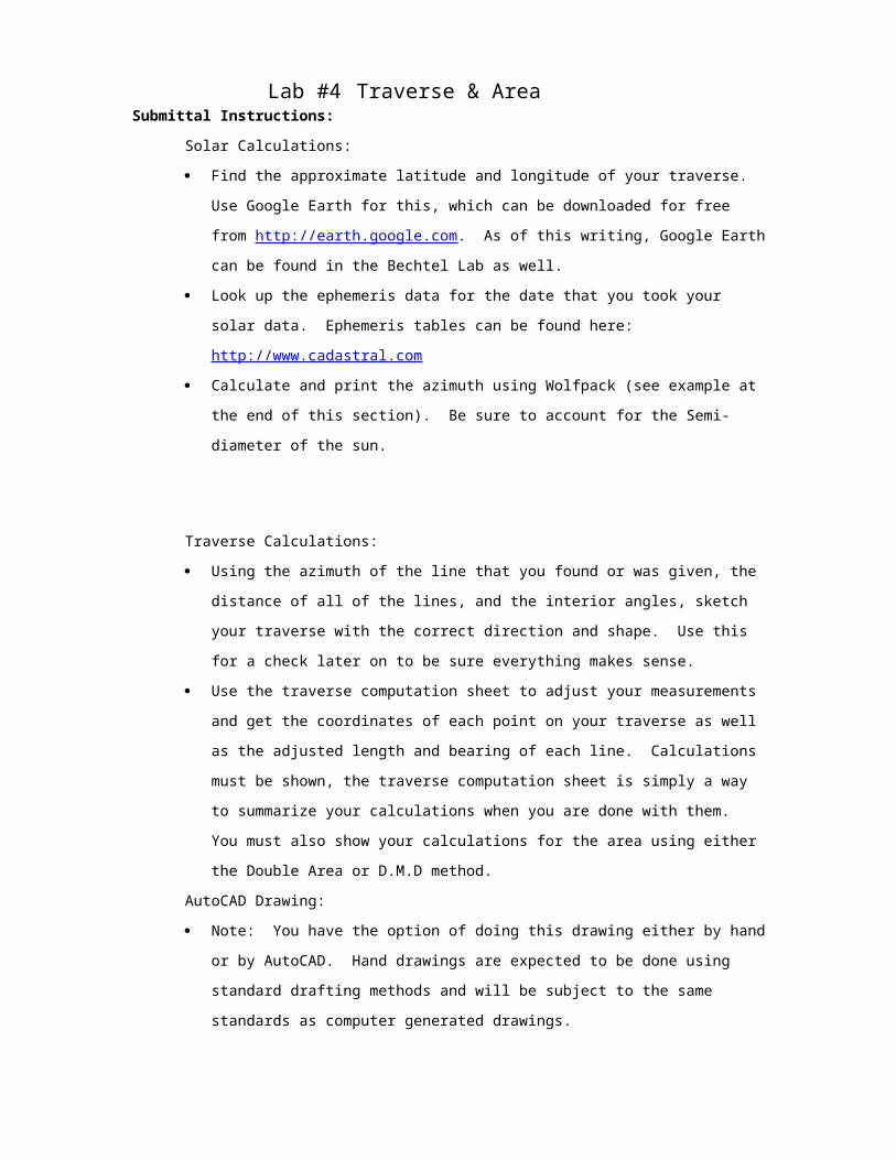
Submittal Instructions:

Solar Calculations:

Find the approximate latitude and longitude of your traverse. Use Google Earth for this,

which can be downloaded for free from http://earth.google.com. As of this writing, Google

Earth can be found in the Bechtel Lab as well.

Look up the ephemeris data for the date that you took your solar data. Ephemeris tables can

be found here: http://www.cadastral.com

Calculate and print the azimuth using Wolfpack (see example at the end of this section). Be

sure to account for the Semi-diameter of the sun.

http://www.cadastral.com/

http://earth.google.com/


Traverse Calculations:

Using the azimuth of the line that you found or was given, the distance of all of the lines, and

the interior angles, sketch your traverse with the correct direction and shape. Use this for a

check later on to be sure everything makes sense.

Use the traverse computation sheet to adjust your measurements and get the coordinates of

each point on your traverse as well as the adjusted length and bearing of each line.

Calculations must be shown, the traverse computation sheet is simply a way to summarize

your calculations when you are done with them. You must also show your calculations for

the area using either the Double Area or D.M.D method.

AutoCAD Drawing:

Note: You have the option of doing this drawing either by hand or by AutoCAD. Hand

drawings are expected to be done using standard drafting methods and will be subject to the

same standards as computer generated drawings.

Your drawing must have a border and title block. The title block should include your name,

crew number, date, course title, course number, your lab time, drawing title, and the scale.

Show the actual traverse, including individually labeled traverse points, length of each

traverse line, and the bearing of each line with the direction of the typing in agreement with

the orientation of the li

ne (a label for a line at N 45 E should be oriented at an angle of 45 degrees from true north

read from left to right)

Once you’ve drawn the traverse lines go to your layout and set your scale to an engineering

scale (1”=10’ 1”=20’ etc). Do NOT use the default font. Create a text style so that the text

in your drawing prints out at either 1/8” or 1/16”, and use City Blueprint as your font. The

default font in AutoCAD is unreadable, and points will be taken off for the overall quality and

readability of your presentation if you do not change the font.

Show the interior angles of your traverse to the nearest second.

Show the north arrow, and the correct, labeled declination for the date specified in your title

block. Here is an example of what the north arrow and declination should look like:

Using Wolfpack to complete Traverse calculations:


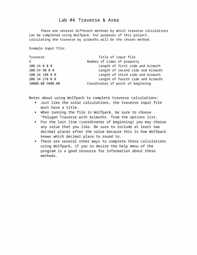
There are several different methods by which traverse calculations can be completed using Wolfpack. For purposes of this project, calculating the traverse by azimuths will be the chosen method.

Example input file:

Traverse Title of input file4 Number of sides of property100.34 0 0 0 Length of first side and Azimuth200.54 90 0 0 Length of second side and Azimuth100.34 180 0 0 Length of third side and Azimuth200.34 270 0 0 Length of fourth side and Azimuth10000.00 5000.00 Coordinates of point of beginning

Notes about using Wolfpack to complete traverse calculations: Just like the solar calculations, the traverse input file must have a title. When running the file in Wolfpack, be sure to choose “Polygon Traverse with Azimuths”

from the options list. For the last line (coordinates of beginning) you may choose any value that you like. Be

sure to include at least two decimal places after the value because this is how Wolfpack knows which decimal place to round to.

There are several other ways to complete these calculations using Wolfpack, if you so desire the help menu of the program is a good resource for information about these methods.


Nam

e:__

____

____

____

____

____

____

_La

b:__

____

____

__ P

arty

:___

____

____

_

Adj

uste

d B

earin

g

____

____

____

____

__

____

____

____

____

__

____

____

____

____

____

____

____

____

____

____

_

Adj

uste

d Le

ngth

Adj

uste

d XY

Adj

uste

d

Dep

artu

re

∑=

Latit

ude

∑=

Tra

vers

e C

ompu

tatio

n Sh

eet

Cor

rect

ion

(Com

pass

Rul

e)

CD

CL

Una

djus

ted

Dep

artu

reL*

sin(

α)

∑=

Latit

ude

L*co

s(α)

∑=

Line

ar M

iscl

osur

e:

Prec

isio

n:

Are

a (f

t2 ,acr

es,m

2 , and

hec

tare

s):

Azi

mut

h(α

)Le

ngth

Uni

ts:_

__

∑=

St a @

Lab #5 DDL (Direct Differential Leveling)

Objectives:

1. Learn and practice rod reading, instrument leveling.

2. Understand Direct Differential Leveling method.

3. Use DDL technique to find unknown elevation of various locations.

Equipment:

1. Leveling Instrument (Telescope)

2. Tripod

3. Rod

4. Field Book

Theory & Method:

Reading the Rod

Rod reading is similar to reading a ruler, the big difference being that the rods for this class are marked

in feet, tenths of a foot, and hundredths of a foot. First, check that the rod is right side up, and that the

numbers are counting upwards from the ground. One side of the rod counts upward from the top of the

rod. This is used for construction surveying and is not needed for this class, so be sure not to

accidentally site to the wrong side of the rod. The smaller black numbers are tenths of a foot. Each

white block and each black block counts as 0.01’. In other words, if you count a white space, a black

line, another white space and another black line, you’ve counted 0.04’, and NOT 0.02’.

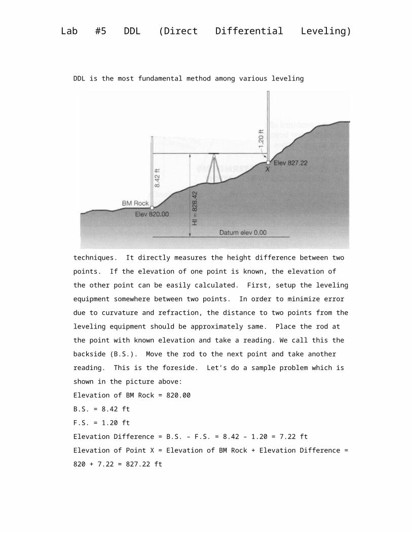
Direct Differential Leveling

DDL is the most fundamental method among various leveling techniques. It directly measures the

height difference between two points. If the elevation of one point is known, the elevation of the other

point can be easily calculated. First, setup the leveling equipment somewhere between two points. In


order to minimize error due to curvature and refraction, the distance to two points from the leveling

equipment should be approximately same. Place the rod at the point with known elevation and take a

reading. We call this the backside (B.S.). Move the rod to the next point and take another reading.

This is the foreside. Let’s do a sample problem which is shown in the picture above:

Elevation of BM Rock = 820.00

B.S. = 8.42 ft

F.S. = 1.20 ft

Elevation Difference = B.S. – F.S. = 8.42 – 1.20 = 7.22 ft

Elevation of Point X = Elevation of BM Rock + Elevation Difference = 820 + 7.22 = 827.22 ft

Lab Procedure:

The goal of this lab is to find the elevation of the four points which are assigned to each group.

Starting from the closest NGS (National Geodetic Survey) benchmark that will be shown to you in lab,

follow the DDL procedure to find the elevation of your four points.

After all four points are found, measure back to your benchmark to check your numbers and calculate

your misclosure. Do not make multiple F.S. measurements from one B.S., otherwise you will run into

trouble calculating your misclosure. If you can not get a reading from one point to the next point

either because it is too far or the slope difference is too big, setup one or several temporary points.


Text page 108

This table is a sample page of field book recording of DDL lab. After this lab you should be able to

construct a table similar to this. You do not need to complete the whole chart during the lab. During the

lab, you only need to record B.S., F.S., and B.M. elevation. The rest can be calculated afterward.


Note Page

Name: ________________________

Crew: ________________________

Date: ________________________

Weather: ________________________

Equipment: ________________________________________________

________________________________________________

Notes: ________________________________________________

________________________________________________

________________________________________________

________________________________________________

________________________________________________

________________________________________________

________________________________________________

________________________________________________________________________________________________

Sketch:


Data Page

STA B.S. H.I. F.S. Elev. Adj. Elev.

Page Check:

Adjustment:

Z

A D

T

R

V

Lab #6 Trigonometric Leveling

Objectives:

1. Practice utilization of a theodolite

2. Understand trigonometric leveling method

3. Use trigonometric leveling technique to find a relative elevation of a building

Equipment:

Theodolite, Tripod, Rod, Tape, and Field Book

Theory & Method:

Calculate the height of a building

Unknown = V,A Measured = R,D,Z

1. V = R + T = R + D * tan A

2. A = 90 – Z

Lab Procedure:

1. Pick a building that you would like to measure the height of

2. Setup the theodolite to where you can see the top of the building. Try to avoid a place right below

the point you would like to site to.

3. Sight to the point on the building that you would like to know the height of. Measure R, D, and Z

(or A). When measuring distance D, note that you must measure to a point directly below where

you are sighting to. This means that you need to site to a point on the outside wall of the building,

otherwise you won’t know where exactly to measure to.

4. Calculate V


Note Page

Name: ________________________

Crew: ________________________

Date: ________________________

Weather: ________________________

Equipment: ________________________________________________

________________________________________________

Notes: ________________________________________________

________________________________________________

________________________________________________

________________________________________________

________________________________________________

________________________________________________

________________________________________________

________________________________________________

________________________________________________

Sketch:


Data Page

R =

D =

Z =

A =

V =

N

X

X

XX

X

X

X

X X

X

X

X

X

X

B

h

A

C

D

Lab #7: Stadia

Objectives:

1. Collect data for approximately 60 to 90 points around your triangular property using total station.

2. Calculate necessary information on your points.

3. Prepare data for use in final project where you will be creating a topographical map with

AutoDesk Land Desktop.

Equipment:

Total Station, tripod, Plumb Bob, Pin, Reflector

Lab Procedure

The Goal is to collect data points so as to construct topographic map around your property lines:

(A) Planimetry Points

1. Planimetry Points are the data points which show locations (Direction, Distance) of various

objects and key landscapes.

2. Location and the number of points is decided based on necessity, where the landscape

changes shape, slope, direction, etc.

3. From a station and backside line, in order to identify a point, two key data is required

Direction () and Distance (h).

(B) Ground Points (G.P)

1. Ground Points are the ground data points which are collected mainly for the purpose of

contour line construction.

2. Set up a data point where the slope changes. For steeper slope use shorter interval.

Lab #7: Stadia

Stadia Computation Sheet (for total station)

Total Station @ _____B.S. @:______ Station Elevation:_________ HI:_______ HR:_______Pt. # Horizontal Angle Zenith Angle

(optional)Horizontal Distance

Vertical Distance Elevation Point Description

Units:B.S.

123456789101112131415161718192021222324252627282930

B.S.

Objectives:

Continue your project with your stadia points and create a topographical map using AutoDesk

Civil 3D .

Project Submittals:

Title page and Table of Contents

Discussion: Discuss briefly any aspects of your data collection that deviated from standard

procedures. Discuss the procedures used in your leveling (loops, error correction) and how they

might affect your topographical results. Identify the objectives of the stadia portion and comment

on your point selection in the field (were the points properly distributed, did you have enough?).

Identify any bad field points that were omitted from the contour generation. Conclude by briefly

commenting on your overall results and what this course has taught you.

DDL Computations: Show BS, FS, HI, elevations, corrected elevations, page check, and

misclosure. Express your data to the nearest hundredth of a foot

Stadia Computations: Include your stadia computation sheets that should have your horizontal

angle, horizontal distance, vertical distance, and elevation filled out. Transform this data into

X,Y,Z coordinates using an Excel spreadsheet. To show your calculations print out your Excel

spreadsheet with the numbers and another with the formulas that you used (CTRL - ~). Your data

should be in the nearest 10th of a foot. Look over the data before importing it into Civil 3D to be

sure that all of the numbers make sense. ( A template spreadsheet can be found on the course

website).

Working Map: The working map is essentially a tool with which you can verify and process your

field data. This map will present ALL the data collected in the field. This initial contour

generation will be modified by manual manipulation of contours and deletion of bad data points.

Information should be legible, although it is expected to be somewhat cluttered. Include the

following on the map:

Traverse stations marked by number and elevation.

You can use the existing 11x17 traverse map and add adjusted DDL elevations to stations.

All stadia points marked by number and elevation

Show all planimetry (trees, paths, ponds, boulders, lights, buildings, etc.) with an

accompanying legend.

Contour Lines generated with Civil 3D

Name Crew number, section number and title.

Use 11 x 17 of larger.

Final Map: The final map is the culmination of all the data you’ve worked to collect. The

majority of the grade will focus on presentation, professionalism, and accuracy. Spend time

making sure things are not cluttered together and all data is clearly legible (no lines through

numbers, etc.). Include the following:

Border and title block, including: name, crew number, date, course number, course title,

section number, scale, project title, and location of traverse (“Part of SW ¼, Sec. 32, T1N,

R70W, 6th P.M.”)

Your traverse lines

Smooth contours (Choose a contour interval that is appropriate for your property). Each fifth

contour should be bold and labeled (0’s and 5’s). Also label any contours that are not

explicitly clear.

Traverse stations marked by number, coordinates, and elevation. Elevations should fall

between correct contours. A separate table in the corner with this data often is the most

readable.

Use 11 x 17 paper .

True north with declination

The final map should be the same as your working map, but it should not show any of the

Stadia points. Use layers in Civil 3D and set up two layouts – one for your working map and

one for your final map. Freeze the points layer in the final map.

Additional requirements are listed in the Civil 3D instructions below.

Original Field Book that is properly marked with name, section number and crew number. The

front page should be filled out, as well as the appropriate notes for each lab. Neatness and

professionalism will be checked (organized, clear, no erasing).

Using Autodesk AutoCAD Civil 3D to complete the Project

It is recommended that each group follow these instructions exactly. Civil 3D is a complicated program, and even doing some of these steps out of order can cause problems. Read through these directions completely first.

- Open Civil 3D - Be sure that the Toolspace is shown on the left of the screen. From the Home tab,

select the Toolspace button if it is missing. The Prospector tab within Toolspace will be used primarily. (The command “showTS” will bring Toolspace back if it accidentally closed.)

- Type in “units” in the command line.- Change the Length Type to Decimal and change the Angle Type to Deg/Min/Sec.

Choose the appropriate precision for each. Check the “Clockwise” box beneath the Angle units to set the default angle measurement to clockwise.

- Ensure that the Insertion Scale is in “Feet.” Click “OK.”

Inserting your points:

- You will need to create a text file (.txt) that contains all of your points, with at least X, Y, and Z coordinates of all of your points.

- Begin with creating an Excel spreadsheet with separate columns for Point #, X, Y, and Z, entering coordinates in feet.

- Copy the point information from the Excel file into a text (.txt) file (the Notepad program in Windows works well for this.) Save your text file so that you can upload it in the coming steps.

- The file should look something like this, with a single space separating each set of numbers along a row.

1 9981.559 5169.746 5349.9322 9971.952 5169.721 5350.0763 9980.167 5169.379 5351.1194 9960.300 5139.925 5350.5415 9961.117 5115.558 5350.702

- For this text file, your traverse points should be assigned a number as well, otherwise the text file will not import into Civil 3D. (101, 102 and 103 work well here).

- Civil 3D allows you to import point files that are formatted in several different ways. The example shown above would be called “PENZ space delimited.”

P = Point NumberE = Easting (X Coordinate)N = Northing (Y Coordinate)D = Optional Point DescriptionZ = Elevation

- To Import Point File into Civil 3D, from the Insert tab, select Points from File. - Ensure that the Format corresponds to the format your text file is set up using. The

example text file above would require “PENZ (space delimited)” to be chosen here. - Click the “+” button on the right and browse for and select your text file. - Click “Add Points to Point Group” and assign a name for your points group (“Final

Project” for example).- Uncheck “Do Elevation Adjustment if Possible.”- Click “OK” to import points.- You should now have a group of points on your screen that are labeled with some small

text.- If you cannot see the points, type the letter “z” (for zoom), press “Enter,” then type the

letters “ex” (for extents) and press “Enter” again. This will zoom in so that the points fill the screen.

- It is suggested that you change your traverse points to a separate layer than your stadia points. The stadia points layer can then be turned “off” when plotting your Final Map later on. To do this, under the Home tab, in the top left of the Layers section, click the Layer Properties button and dock the Layer Properties Manager to the right of the screen. Click the New Layer button within the Layer Properties Manager and name the new layer whatever you choose.

- Select your three traverse points (you likely have assigned a number to these in the text file) and right click and choose Properties. Under the Layer option, assign these points to the new layer you have just created.

- To turn a layer on or off, in the Layer Properties Manager, click the Lightbulb icon off. If the layer is still displayed, you may also need to turn off the “Freeze” button for the layer.

Select your plotting scale: - Click on the “Layout 1” button in the bottom right of the screen:

- Click the File button, then under Print, Select Page Setup

“File” button

- Click the Modify button while Layout 1 is highlighted. - Choose your printer/plotter (you can also plot to an Adobe PDF, depending on whether

it is installed on the computer you are using).- Select the paper size you plan to plot on. (11x17/tabloid or larger is required)- Pick Portrait or Landscape layout, whichever best matches your group of points.- Set your Plot Style to Monochrome.- Click “OK” and close the Page Setup Manager.- Resize your viewport, leaving enough room for a title block.- Change the scale to a suitable scale. 1” = 10’, 1” = 20’, 1” = 30’. Note: 1:10 is NOT

the same as 1” = 10’.- Center the plot, being careful not to change the scale by zooming in or out.

Altering Your Point Labels:

- Individual Point Labels can be clicked and dragged by clicking on a point and clicking and dragging the blue box on the right. Civil 3D will automatically add a leader line and arrow to the point.

Create Text Styles:

- Now that you know what scale you are going to plot in, you can deal with text styles. Standard text styles should be used for your drawing (1/16”, 1/8” or 1/4”). City Blueprint is REQUIRED to be used as the font for this drawing.

- Your annotation scale should be set first. Under the Home tab, Palettes menu, select Properties. (You must be in model space to do this.)

- Select the scale you chose for your viewport in Layer 1. If the scale you chose is not present, select “Custom” and create the scale.

- The annotation scale should be set in both model space, and for each viewport. To change the Annotation Scale for the viewport, go to the layout and select the viewport. The Annotation Scale can now be changed under the Properties menu.

- Type “style” into the command line.- Set the font to “City Blueprint” for all of the text styles that are listed.

Display Contour Lines:

- From the Prospector tab of the Toolspace menu, right click on “Surfaces” and click “Create Surface.” Click “OK” to accept the defaults.

- Expand the Surface, the Surface 1, and then the Definitions menus. - Right Click on Point Groups and click “Add.”- Select the point group that you created when you imported your points and click “OK.”- Right Click on Surface 1 and click “Edit Surface Style.”- Under the Contours tab, contour properties can be adjusted. Under Contour Intervals,

adjust the major and minor intervals to best represent your topography. Under Contour Smoothing, change Smooth Contours from “False” to “True.”

- To remove the border from the surface, under the Borders tab, Border Types menu, change Display Exterior Borders from “True” to “False.”

- Change other contour settings as appropriate.- To remove a point from the surface, click on the point, right click on the point, and

select “Point Group Properties.” Under the Exclude tab, type in the point number(s) you wish to exclude from the surface and click “OK.” The surface will need to then be rebuilt by right clicking on Surface 1 and clicking “Rebuild.”

- Add contour labels: Select a contour, and the surface will be selected. The “Tin Surface” tab will be automatically selected, then click “add labels” on the top left side of the ribbon and from the drop-down list select “Contour – Multiple”. Then select the contour lines at points where you want to label with contour elevations. It is typical to label the major intervals only, not every contour line. If you have selected an appropriate annotation scale as described earlier, the contour labels will appear at an acceptable scale.

- Contour lines should be edited to reflect the actual contours crossing roads and sidewalks. The best way to achieve this is by using breaklines. Use the polyline command to outline streets or sidewalks on each side; this line will be used as a breakline to define the AutoCAD surface definition across the relatively flat road or sidewalk.

Hints for the final project and Civil 3D:

Often there will be one or two points within your stadia data that drastically alter the accuracy and aesthetic of your contour surface. To fix this problem the offending points must be deleted. Double check your XYZ input file for any outlying values and adjust the points list in Civil 3D accordingly. (The procedure for altering the points can be found on the previous page.)

To include planimetry for your final map, the AutoCAD Design Center maybe used. This is a library of pre-drawn surveying symbols and other landscaping symbols that can be directly inserted into your map. The help section of AutoCAD Civil 3D is a valuable resource for further information about the Design Center.

Hints for GIS Lab exercises:

To register with ESRI:

1. Go To My TrainingGo to http://training.esri.com. Click "Go to My Training." Under My Courses click "My Virtual Campus Courses." If you already have an ESRI Global Account, log in using your username and password. If you do not, click "Create New Account." 2. Start Your New CourseClick "Start a new course". Type your 14-character Course Access Code in the field provided and click "Go." Follow the instructions on your screen. (This code will be provided in lab) 3. Go To ClassFrom your course list, click the course title to begin.

Tips for Map due in Lab 1:

· Complete Exercise (Find Potential Youth Center Locations) through step 6. You should now have the potential youth center locations. Do NOT apply the map template.

· Insert – New Data Frame· Copy and Paste Layers in the New Data Frame· Use one Data Frame for a Small Map (zoomed out to full extent) and one Data

Frame for a Large Map (zoomed in to potential youth center locations).· Switch to the Layout View· Create your map with Title, Data Frames, Legend, Scale Bars, Name, North

Arrow (under Insert header)· Another tip is to remember going to Layer Properties (Rt-Click on the Layer) and

choose the Labels tab to edit the labels (size, appearance, etc.) (also change layer name) - Make labels easy to read! To save your map, DO NOT save it as an .mxd file. Go to File, Export Map, then save file as a JPEG. Show the jpeg in class or email to Dr. McCluskey.

Tips for Map due in Lab 2:· Complete Module 1 of Spatial Analysis Course· Complete Last Exercise (Reclassify Data to a Common Scale)· Convert Layer to Vector (ToolBox – Conversion Tools; From Raster; Raster To

Polygon)· Go to Symbology (under Layer Properties); Choose Categories, Unique Values,

Use GRIDCODE as Value Field, Add All Values, click on each block to change the symbology and change the labels to show both vegetation type and drought tolerance number

· Only need 1 data frame, but still need Title, Name, scale bar, north arrow, and legend

· Export map and save as JPEG then email to me or show me in lab

The final lab tutorial and data are located at: http://alovintouch.com/GEOMATICS Both files need to be downloaded (SurvData.zip & Surveydata_GIS.zip) for the final lab exercises. Tips and requirements for this lab can be found in the tutorial file. GIS Review for second midterm exam:

• GIS• GIS Analysis• Spatial Data/Attribute Data• Vector and Raster Data• Elements of a good map• ArcGIS Desktop (ArcMap, ArcCatalog, ArcToolbox)• Large and Small Scale Maps• Attribute Table• Metadata• Layout and Data View• Symbology• Geoprocessing• Reclassifiying• Classifications Used in Lab 2• Survey Aware Features• Sub-layers• LINK Tool in Lab3 There will be some general questions about what you did during the labs (possibly similar to the exam questions at the end of the modules/courses.) The lectures are posted on the class web page.You can review them for help with some of the terms you may also review the on-line tutorials.

Lab #5 DDL (Direct Differential Leveling)bechtel.colorado.edu/~halek/Spring_2016_Field_Book.docx ·...

Documents

Transcript of Lab #5 DDL (Direct Differential Leveling)bechtel.colorado.edu/~halek/Spring_2016_Field_Book.docx ·...