Lab #2 – GIS Overlay Analysis NR506 – Advanced GIS Applications in Fire Ecology and Management Objectives

• Utilize GIS tools for overlay analysis – ArcView 3x, ArcGIS 8x, ArcInfo • Become more comfortable working with ArcMap 8.3 • Explore techniques for overlay analysis between point, polygon and raster data • Understanding conditional probabilities • Explore overlay analysis techniques related to fire GIS data

Set up the ArcMap project All data for this lab is located in folder c:/NR506/data/selway All data in this folder is in projection: UTM, Zone 11, datum NAD27, map units meters 1. Open ArcMap with a new map: – Programs - Start – ArcGIS – ArcMap – OK 2. Select File – Add data. Add the following datasets: dataset description data type scale/resolution sbw_pvt Potential Vegetation Types (PVTs) for

the Selway-Bitterrot Wilderness grid 30 m pixels

sbw_ele Elevation for the Selway-Bitterrot Wilderness

grid 30 m pixels

firestarts_selway_1986-1992.shp

Fire start locations year 1996-1992. ICRB project (USFS + BLM)

shapefile

huc5.shp 5th order watersheds in the Selway-Bitterrot area

shapefile 1:100,000

Fires2000 Fire perimeters burned in year 2000 coverage 1:100,000 idahobnd Idaho state boundary coverage 1:100,000 Pvt.dbf PVT code look-up table DBASE Build pyramids for the two grids (increases the display speed when zooming in or out). Order the datasets in the layer table by moving them up or down. Layers can only be moved when Display in the lower left corner is selected. Add extensions: Select Extensions in the Tools menu on top; Check Spatial Analyst and Xtools; Close the Extensions dialog box. Display the toolbars for Spatial Analyst and Xtools by selecting them under the Toolbars option in the View menu. SAVE the ArcMap project!

1

Q 51 Rt

3. Join the PVT code lookup table to the PVT grid. The table pvt.dbf contains descriptions of the numeric PVT codes. This join will enable you to display the vegetation types with a description instead of a numeric code. Right click on the sbw_pvt data layer; select Joins and Relates; select join; enter values according to the dialog box to the right. NOTE: The VALUE in the sbw_pvt table and PVT_CODE in the pvt.dbf table are the ‘join attributes’. These attributes represent the same numeric code for a Potential Vegetation Type (PVT). Click OK.

4. Working with Layer Properties (editing legends) for display. Right click on the sbw_pvt data layer; select Properties; click on the Symbology tab on top; Choose to display the data as ‘Unique Value’ (upper left); select pvt.PVT_NAME for the Value Field; click ‘Add All Values’ To change the symbol colors, double-click on the symbol and then select a color. Click OK.

uery a GIS database

. Question #1: How many fires started in the Selway –Bitterrot Wilderness in the time period 986 – 1992? ight-click on the layer ‘firestarts_selway_1986-1992’; select Open Attribute Table; record the

otal number of fire starts in the table (see the lower bar of the table).

2

Question #2: How many of those fires have a final size larger than 1000 acres? Click Options on the lower bar of the table ; click Select by Attributes. In the Select Attributes dialog box: double-click on FINALSIZE; click > (greater than); type 1000; click ‘Apply’. Record the number of fire starts with a final size larger than 1000 acres (see the lower bar of the table). Close the dialog box and the table. Notice that the fires larger than 1000 acres are displayed on the map. Clear selected features: Right-click on the layer ‘firestarts_selway_1986-1992’ – select Selection – Clear selected features Make a summary table using Xtools in ArcMap

Xtools is a ‘third party’ extension for ArcMap free for download at: http://arcscripts.esri.com/details.asp?dbid=11731. At this site you can also read more about the tool. In this exercise we will use Xtools to summarize occurrences of fire causes (lightning, smoking, etc.) in the Selway-Bitterrot Wilderness area and summarize how much area burned by fire cause. Xtools is a useful tool and will be used frequently throughout this course. Summary tables can also be created using the Summarize Tool (right-click on a table attribute and select Summarize…), however these summations can only be applied to one single variable while Xtools can perform multiple summations.

Question #3 : What are the four causes of fire starts in the Selway-Bitterrot Wilderness 1986-1992?

Fire start codes used in the attribute table for the layer ‘firestarts_selway_1986-1992’, attribute FIRE_CAUSE. 1 LIGHTNING 2 ARSON 3 SMOKING 4 RECREATION 5 CHILDREN 6 DEBRIS BURNING 7 EQUIPMENT USE 8 RAILROAD 9 MISCELLANEOUS See metadata c:/nr506/data/selway/firestarts_selway_1986-1992_metadata.dat for further information.

6. Start the frequency table tool in Xtools by selecting Xtools – Table Operations – Multiple summarizations.

Summarize Wizard (Step1 of 3): Input layer: Firestarts_selway_1986-1992 Output: Browse and name the output table

3

Summarize Wizard (Step 2 of 3) Select FIRE_CAUSE and click the arrow pointing to the right. Xtools will sum all unique occurrences of fire causes

Question #4 : How many percent of the fires we

How much area (finalsize is exp

Summarize Wizard (Step 3 of 3) Select FINALSIZE and click the arrow pointing to the right. FINALSIZE is expressed in acres. Xtools will sum the final sizes of fires for eachunique occurrences of fire causes. Click Finish to produce the final frequency table. Use the information in the table to answer question #4 below.

re caused by lightning? ressed in acres) was burned due to recreation?

Save your ArcMap project periodically - ArcMap WILL eventually crash!(just like everything will eventually burn ☺)

4

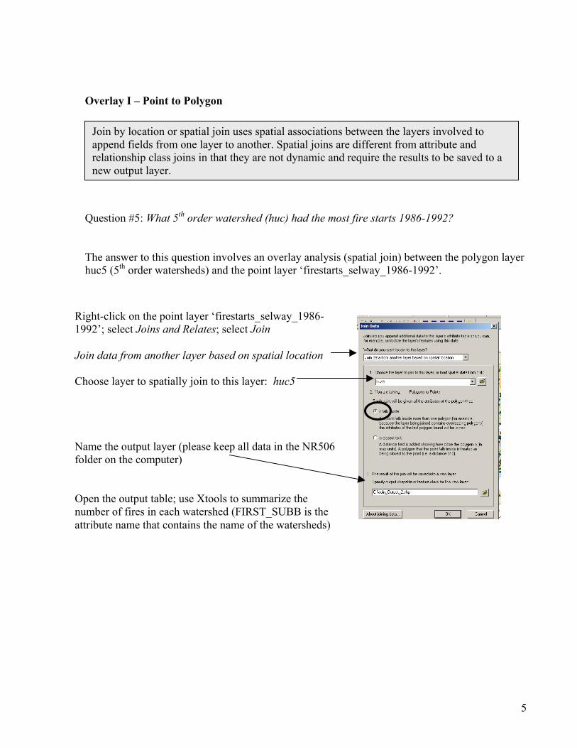
Overlay I – Point to Polygon

Join by location or spatial join uses spatial associations between the layers involved to append fields from one layer to another. Spatial joins are different from attribute and relationship class joins in that they are not dynamic and require the results to be saved to a new output layer.

Question #5: What 5th order watershed (huc) had the most fire starts 1986-1992? The answer to this question involves an overlay analysis (spatial join) between the polygon layer huc5 (5th order watersheds) and the point layer ‘firestarts_selway_1986-1992’.

Right-click on the point layer ‘firestarts_selway_1986-1992’; select Joins and Relates; select Join Join data from another layer based on spatial location Choose layer to spatially join to this layer: huc5 Name the output layer (please keep all data in the NR506 folder on the computer) Open the output table; use Xtools to summarize the number of fires in each watershed (FIRST_SUBB is the attribute name that contains the name of the watersheds)

5

8. Derive slope and aspect from the elevation layer (sbw_ele) The Spatial Analyst must be turned on in order to perform raster analysis in ArcGIS ( Tools – Extension, check Spatial Analyst). Also, the Spatial Analyst toolbar must be added to the project (View – Toolbars, check Spatial Analyst). First, select Options in the Spatial Analyst menu and define the Working directory (c:/nr506/data/selway), analysis mask (sbw_ele), extent (same as sbw_ele) and cell size (same as sbw_ele, 30 m).

Make sure that sbw_ele is the ‘active layer’ in the Spatial Analyst toolbar.

Select Surface Analysis in the Spatial Analyst drop down menu. Derive Slope (in degrees, z factor 1, cell size 30 and save the slope grid as c:/nr506/data/selway/sbw_slope) Derive Aspect (input surface is sbw_ele, cell size is 30 m, save the slope grid as c:/nr506/data/selway/sbw_aspect) Use the Layer Properties (right-click on the layer and select Properties) for sbw_slope and sbw_aspect to display the layer legends as you wish.

Save your ArcMap project periodically - ArcMap WILL eventually crash!☺

6

Overlay Analysis II – Point to Grid

The spatial join procedure described above only works when relating points to polygons. You can relate points to grids (raster data) using the Raster Calculator in the Spatial Analyst extension. A point layer can be related to multiple grids (slope, elevation, aspect, vegetation etc. ) simultaneously by using the SAMPLE command.

Question #6: How many fires started in each one of the Potential Vegetation Types 1986-1992? How much area is there in each PVT in the Selway – Bitterrrot Wilderness? Also, calculate the ratio between ‘% fire starts in PVT’ and ‘%area in PVT’ (if the ratio is larger than one more fires than expected start in this PVT).

pvt_code pvt_name # of firestarts

2 Western Red Cedar 3 Grand Fir 4 Douglas-fir 5 Lower Subalpine Moist 6 Lower Subalpine Dry 7 Upper Subalpine Moist 8 Upper Subalpine Dry 9 Persistent Herblands

10 Rock/Alpine/Barren land 11 Water

Question #7: What PVT has the highest # o What PVT has the highest # of 9. In order to answer question #6 and #7 ab

locations and then use the Raster Calculatslope and aspect each one of the fire start

Create a point-grid from firestarts_selwa1992.shp by selecting Convert in the Spadrop down menu; then select Feature toInput feature: firestarts_selway_1986-1Field: ID (unique id for each fire start loOutput cell size: 30 Output raster: c:\NR506\data\selway\f

Area (m2) = Count x 30 x 30 Count can be found in the PVT attribute table – count is the number of pixels (cells) in the grid with a certain value30 m is the cell size

% of fires started in PVT (%1)

Area in PVT

% area in PVT (%2)

Ratio (%1) /( %2)

f fire starts? fire starts in relation to its area?

ove we will create a point-grid from the fire start or in Spatial Analyst to find out what PVT, elevation, locations is located in.

7

y_1986-tial Analyst

raster; 992.shp cation)

irestart_id

Select Raster Calculator in the Spatial Analyst drop-down menu.

Enter the expression below in the Raster Calculator window. SAMPLE is a command that works in both ArcINFO Workstation and in the Spatial Analyst Raster Calculator. See Arc Workstation Documentation for more information on this command. A tab delimited text table named fire_data.txt is created. This table contains the fire ID number, along with PVT, elevation, aspect and slope for each fire start. This table can be a basis for further statistical analysis.

fire_data.txt = SAMPLE([FIRESTARTS_ID],[sbw_pvt],[sbw_ele],[sbw_aspect],[sbw_slope])

Work with the table fire_data.txt in Microsoft EXCEL to find the answers to Question #6 and #7. (You can also bring the table into EXCEL, save as a .dbf file, do the table analysis using Xtools in ArcMap).

8

Overlay III – Polygon on Grid

Np

The Zonal Statistics option in the Spatial Analyst extension is a useful tool for poly-grid or grid-grid overlay analysis. Zonal Statistics computes statistics such as minimum, maximum, mean, range etc. of continuous data (such as elevation of slope) within a zone defined by a zonegrid (or polygon cover).

Question #8: What is the min, max and averages elevation in the two watersheds White Cap Creek and Moose Creek? Watershed Min elevation, m Max elevation, m Mean elevation, m White Cap Creek Moose Creek Select Zonal Statistics in the Spatial Analyst drop down menu.

Zone dataset: huc5 (watersheds) Zone field: FIRST_SUBB (name of watershed) Value raster: sbw_ele (elevation layer) Output table: whatever you want to name it The output will be a .dbf table containing the zonal statistics (min, max, mean, range, etc.) for the value raster theme within each zone.

OTE: The Tabulate Areas option in Spatial Analyst for ArcView 3.x is also a useful tool for oly to grid overlay analysis. Unfortunately this option was removed in ArcGIS 8.x.

Question #9: How would you calculate the percent of each PVT within the Moose Creek watershed? (you don’t have to do this, simply explain how you would approach this problem using GIS - any tool is OK).

9

Overlay IV – Grid to Grid Question #10: Where are areas of Douglas-fir (pvt 4) on Flat, North, East, South and Western aspects? How much area is there? Express the areas in hectares (count x 30 x 30 / 10000) PVT Flat North East South West Douglas-fir GIS overlay analysis is a useful tool in planning and stratifying sampling locations for vegetation and fuels. In this example we are planning a stratified sampling procedure by aspect (n, e, s, w) and PVT. 10. Reclassify aspect into five classes; Flat, North, East, South and West.

Type in the ‘old values’ and ‘new values’ according to the dialog box to the left. The reclassified grid will have 5 categories (values): 1 – Flat (-1) 2 – North (0 – 45 ; 315 - 360) 3 – East (45 - 135) 4 – South (135 - 225) 5 – West (225 - 315) When typing the ‘old values’ there MUST be a space between numbers and dashes (see above) Name the output raster (asp_reclass for example) OK

Semi-colon

Select Reclassify in the Spatial Analyst drop down menu; select your aspect grid for the input raster and the Value for the reclass field; Click Classify In the Classification dialog box, select Method Equal interval with 5 classes (flat, north, east, south, west) Click OK

10

11. You are now ready to combine the two data layers (grids) asp_reclass and PVT to be able to find stratified sampling locations by aspect and PVT for your fuel sampling. Open the Raster calculator in Spatial Analyst. Enter the following command:

asp_pvt = combine([sbw_pvt], [asp_reclass]) Click Evaluate Asp_pvt is the name of the output grid, COMBINE is an ArcINFO command. The output grid (asp_pvt) is a grid that contains each unique combination of aspect class and PVT. Open the attribute table for asp_pvt and find the answer to Question #10.

11

GIS Overlay Analysis – cheat sheet Eva Strand, CNR, Remote Sensing and GIS Teaching lab, NR506, Fall 2003

Overlay type ArcView 3x ArcMap 8x ArcInfo Workstation Point to Polygon

Geoprocessing Wizard – Spatial Join Animal movement – classify point by poly

Right-click on point layer: Join and Relates – Join – Join data based on spatial location

Arc: identity

Point to Grid Spatial Analyst: Analysis – Tabulate Areas

or Script: samplegrids.ave

Spatial Analyst: Raster Calculator Use the SAMPLE command as you would in ArcInfo- GIRD

GRID: sample

Poly to Poly Geoprocessing Wizard – Intersect or Union Clip one polygon cover based on another (Geoprocessing Wizard)

Geoprocessing Wizard – Intersect or Union Clip one polygon cover based on another (Geoprocessing Wizard)

Arc: intersect or

Arc: union or

Arc: identity

Poly to Grid Spatial Analyst: Analysis – Tabulate Areas Spatial Analyst – Zonal Statistics Clip the grid with a polygon layer: Grid Analyst extension

Convert poly to grid or grid to poly and use the poly to poly or grid to grid overlay Spatial Analyst – Zonal Statistics Mask the grid with a polygon layer (first convert poly to grid)

GRID: zonalstats Mask the grid with a polygon layer (first convert poly to grid)

Grid to Grid Spatial Analyst: Analysis – Tabulate Areas

or Extension: Grid Transformations Tools – Transform Grids – Combine Mask one grid with the other

Spatial Analyst: Raster Calculator: Combine(grid1, grid2) Spatial Analyst – Zonal Statistics Mask one grid with the other

GRID: combine GRID: zonalstats Mask one grid with the other

12

Lab #2 – GIS Overlay Analysis NR506 – Advanced GIS Applications in Fire Ecology and Management Question #1: How many fires started in the Selway –Bitterrot Wilderness in the time period 1986 – 1992? Question #2: How many of those fires have a final size larger than 1000 acres? Question #3 : What are the four causes of fire starts in the Selway-Bitterrot Wilderness 1986-1992? Question #4 : How many percent of the fires were caused by lightning?

How much area (finalsize is expressed in acres) was burned due to recreation?

Question #5: What 5th order watershed (huc) had the most fire starts 1982-1992? How many fire starts? Question #6: How many fires started in each one of the Potential Vegetation Types 1986-1992? How much area is there in each PVT in the Selway – Bitterrrot Wilderness? Also, calculate the ratio between ‘% fire starts in PVT’ and ‘%area in PVT’ (if the ratio is larger than one more fires than expected start in this PVT).

pvt_code pvt_name # of fire starts

% of fires started in PVT (%1)

Area in PVT

% area in PVT (%2)

Ratio (%1) /( %2)

2 Western Red Cedar 3 Grand Fir 4 Douglas-fir 5 Lower Subalpine Moist 6 Lower Subalpine Dry 7 Upper Subalpine Moist 8 Upper Subalpine Dry 9 Persistent Herblands

10 Rock/Alpine/Barren land 11 Water

Question #7: What PVT has the highest # of fire starts? What PVT has the highest # of fire starts in relation to its area?

13

Question #8: What is the min, max and averages elevation in the two watersheds White Cap Creek and Moose Creek? Watershed Min elevation, m Max elevation, m Mean elevation, m White Cap Creek Moose Creek Question #9: How would you calculate the percent of each PVT within the Moose Creek watershed? (you don’t have to do this, simply explain how you would approach this problem using GIS - any tool is OK). Question #10: Where are areas of Douglas-fir (PVT 4) on Flat, North, East, South and Western aspects? How much area is there? Express the areas in hectares (count x 30 x 30 / 10000) PVT Flat North East South West Douglas-fir

14