Lab 12 Gaussian Quadrature - BYU ACMELab 12 Gaussian Quadrature Lab Objective: Numerical quadrature...
5
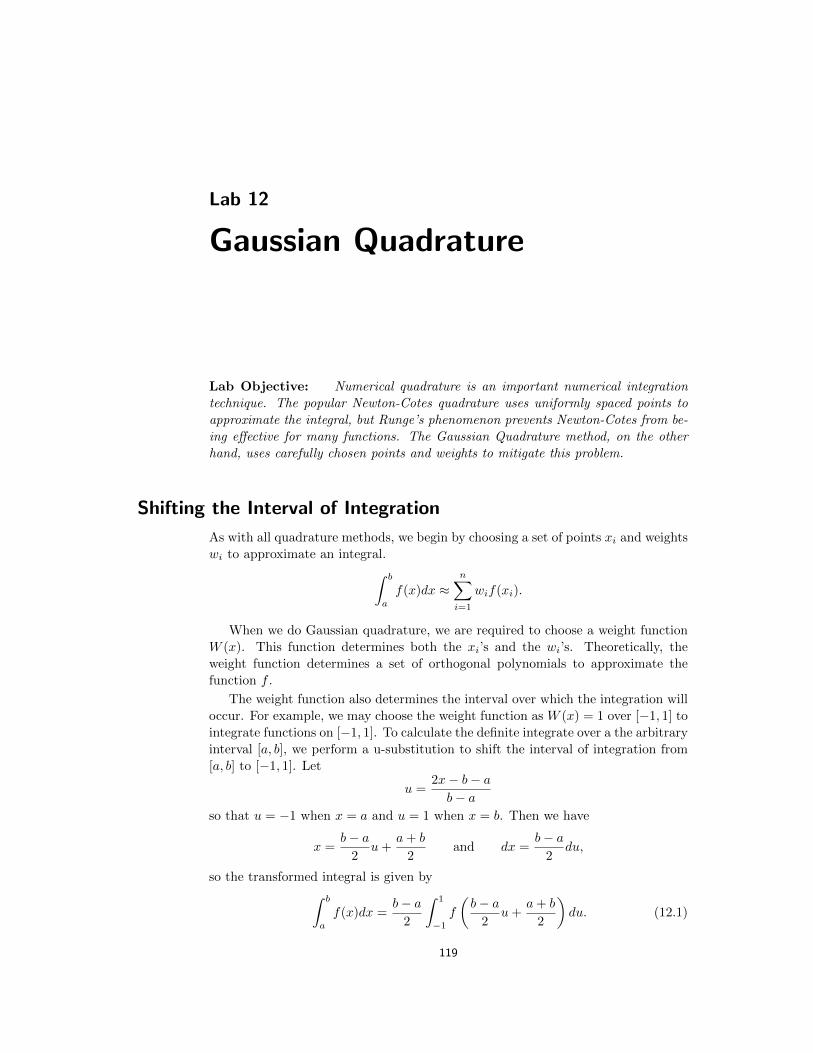
Lab 12 Gaussian Quadrature Lab Objective: Numerical quadrature is an important numerical integration technique. The popular Newton-Cotes quadrature uses uniformly spaced points to approximate the integral, but Runge’s phenomenon prevents Newton-Cotes from be- ing e↵ective for many functions. The Gaussian Quadrature method, on the other hand, uses carefully chosen points and weights to mitigate this problem. Shifting the Interval of Integration As with all quadrature methods, we begin by choosing a set of points x i and weights w i to approximate an integral. Z b a f (x)dx ⇡ n X i=1 w i f (x i ). When we do Gaussian quadrature, we are required to choose a weight function W (x). This function determines both the x i ’s and the w i ’s. Theoretically, the weight function determines a set of orthogonal polynomials to approximate the function f . The weight function also determines the interval over which the integration will occur. For example, we may choose the weight function as W (x) = 1 over [-1, 1] to integrate functions on [-1, 1]. To calculate the definite integrate over a the arbitrary interval [a, b], we perform a u-substitution to shift the interval of integration from [a, b] to [-1, 1]. Let u = 2x - b - a b - a so that u = -1 when x = a and u = 1 when x = b. Then we have x = b - a 2 u + a + b 2 and dx = b - a 2 du, so the transformed integral is given by Z b a f (x)dx = b - a 2 Z 1 -1 f ✓ b - a 2 u + a + b 2 ◆ du. (12.1) 119
Transcript of Lab 12 Gaussian Quadrature - BYU ACMELab 12 Gaussian Quadrature Lab Objective: Numerical quadrature...
Lab 12
Gaussian Quadrature
Lab Objective: Numerical quadrature is an important numerical integrationtechnique. The popular Newton-Cotes quadrature uses uniformly spaced points toapproximate the integral, but Runge’s phenomenon prevents Newton-Cotes from be-ing e↵ective for many functions. The Gaussian Quadrature method, on the otherhand, uses carefully chosen points and weights to mitigate this problem.
Shifting the Interval of Integration
As with all quadrature methods, we begin by choosing a set of points xi
and weightsw
i
to approximate an integral.
Zb
a
f(x)dx ⇡nX
i=1
wi
f(xi
).
When we do Gaussian quadrature, we are required to choose a weight functionW (x). This function determines both the x
i
’s and the wi
’s. Theoretically, theweight function determines a set of orthogonal polynomials to approximate thefunction f .
The weight function also determines the interval over which the integration willoccur. For example, we may choose the weight function as W (x) = 1 over [�1, 1] tointegrate functions on [�1, 1]. To calculate the definite integrate over a the arbitraryinterval [a, b], we perform a u-substitution to shift the interval of integration from[a, b] to [�1, 1]. Let
u =2x� b� a
b� a
so that u = �1 when x = a and u = 1 when x = b. Then we have
x =b� a
2u+
a+ b
2and dx =
b� a
2du,
so the transformed integral is given byZ
b
a
f(x)dx =b� a
2
Z 1
�1f
✓b� a
2u+
a+ b
2
◆du. (12.1)
119

120 Lab 12. Gaussian Quadrature
The general quadrature formula is then given by the following equation.Z
b
a
f(x)dx ⇡ b� a
2
X
i
wi
f
✓(b� a)
2xi
+(a+ b)
2
◆
Problem 1. Write a function that accepts a function f , interval endpointsa and b, and a keyword argument plot that defaults to False. Use (12.1) toconstruct a function g such that
Zb
a
f(x)dx =b� a
2
Z 1
�1g(u)du.
(Hint: this can be done in a single line using the lambda keyword.)
If plot is True, plot f over [a, b] and g over [�1, 1] in separate subplots. Thefunctions probably have similar shapes, but note the di↵erence in the scalingof the y-axis. Try f(x) = x2 and f(x) = (x� 3)3 over 1, 4] as examples.
Finally, return the new function g.
Integrating with Given Weights and Points
With the new shifted function g from Problem 1, we can write the quadratureformula as follows. Z
b
a
f(x)dx ⇡ b� a
2
X
i
wi
g(xi
) (12.2)
Suppose for a given weight function W (x) and a given number of points n, wehave the sample points x = [x1, . . . , xn
]T and weights w = [w1, . . . , wn
]T stored as1-d NumPy arrays. The summation in (12.2) can then be calculated with the vectormultiplication wTg(x), where g(x) = [g(x1), . . . , g(xn
)]T.
Problem 2. Write a function that accepts a function f , interval endpointsa and b, an array of points x, and an array of weights w. Use (12.2) and yourfunction from Problem 1 to calculate the integral of f over [a, b]. Return thevalue of the integral.
To test this function, use the following 5 points and weights that accom-pany the constant weight function W (x) = 1 (this weight function corre-sponds to the Legendre polynomials). See the next page for their definitionsusing NumPy.
xi
� 13
r5 + 2
q107 � 1
3
r5� 2
q107 0 1
3
r5� 2
q107
13
r5 + 2
q107
wi
322� 13p70
900
322 + 13p70
900
128
225
322 + 13p70
900
322� 13p70
900
121
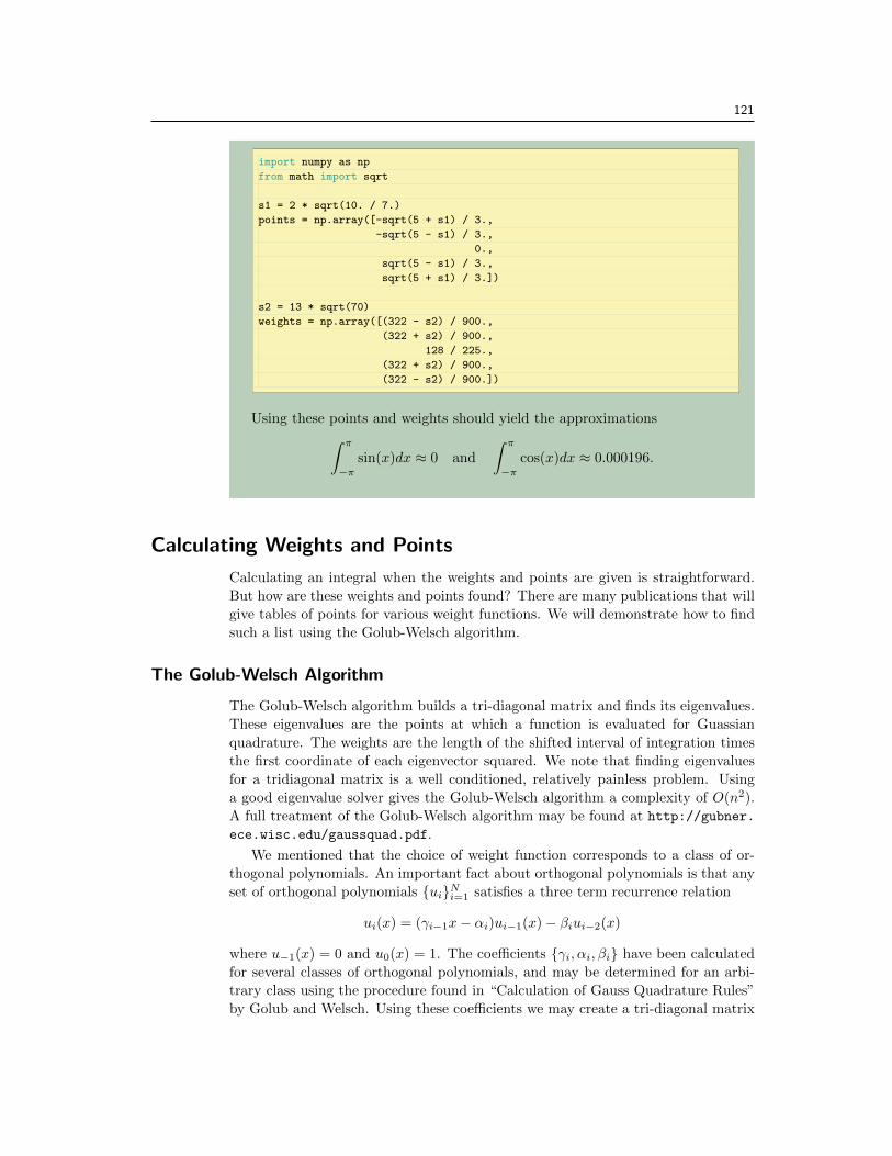
import numpy as np
from math import sqrt
s1 = 2 * sqrt(10. / 7.)
points = np.array([-sqrt(5 + s1) / 3.,
-sqrt(5 - s1) / 3.,
0.,
sqrt(5 - s1) / 3.,
sqrt(5 + s1) / 3.])
s2 = 13 * sqrt(70)
weights = np.array([(322 - s2) / 900.,
(322 + s2) / 900.,
128 / 225.,
(322 + s2) / 900.,
(322 - s2) / 900.])
Using these points and weights should yield the approximations
Z⇡
�⇡
sin(x)dx ⇡ 0 and
Z⇡
�⇡
cos(x)dx ⇡ 0.000196.
Calculating Weights and Points
Calculating an integral when the weights and points are given is straightforward.But how are these weights and points found? There are many publications that willgive tables of points for various weight functions. We will demonstrate how to findsuch a list using the Golub-Welsch algorithm.
The Golub-Welsch Algorithm
The Golub-Welsch algorithm builds a tri-diagonal matrix and finds its eigenvalues.These eigenvalues are the points at which a function is evaluated for Guassianquadrature. The weights are the length of the shifted interval of integration timesthe first coordinate of each eigenvector squared. We note that finding eigenvaluesfor a tridiagonal matrix is a well conditioned, relatively painless problem. Usinga good eigenvalue solver gives the Golub-Welsch algorithm a complexity of O(n2).A full treatment of the Golub-Welsch algorithm may be found at http://gubner.ece.wisc.edu/gaussquad.pdf.
We mentioned that the choice of weight function corresponds to a class of or-thogonal polynomials. An important fact about orthogonal polynomials is that anyset of orthogonal polynomials {u
i
}Ni=1 satisfies a three term recurrence relation
ui
(x) = (�i�1x� ↵
i
)ui�1(x)� �
i
ui�2(x)
where u�1(x) = 0 and u0(x) = 1. The coe�cients {�i
,↵i
,�i
} have been calculatedfor several classes of orthogonal polynomials, and may be determined for an arbi-trary class using the procedure found in “Calculation of Gauss Quadrature Rules”by Golub and Welsch. Using these coe�cients we may create a tri-diagonal matrix
122 Lab 12. Gaussian Quadrature
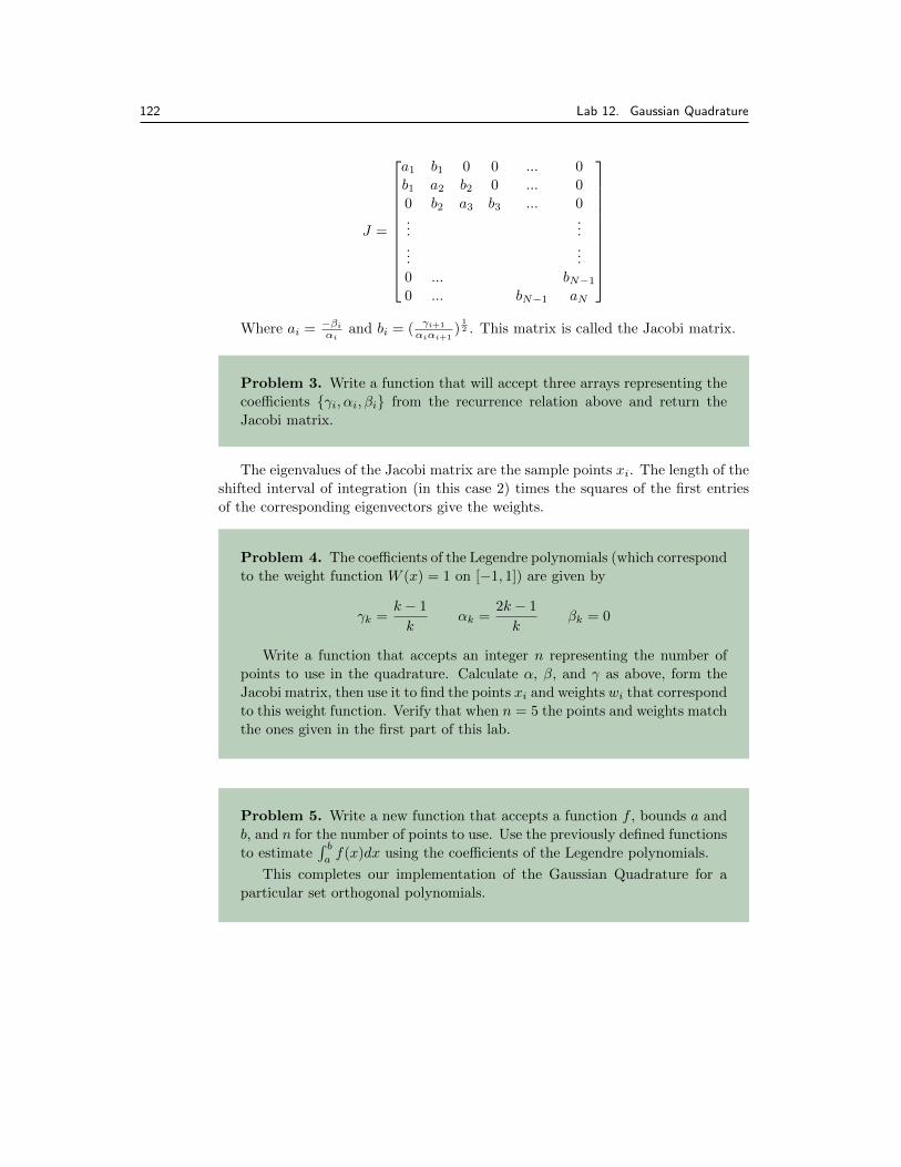
J =
2
66666666664
a1 b1 0 0 ... 0b1 a2 b2 0 ... 00 b2 a3 b3 ... 0...
......
...0 ... b
N�1
0 ... bN�1 a
N
3
77777777775
Where ai
= ��i
↵iand b
i
= ( �i+1
↵i↵i+1)
12 . This matrix is called the Jacobi matrix.
Problem 3. Write a function that will accept three arrays representing thecoe�cients {�
i
,↵i
,�i
} from the recurrence relation above and return theJacobi matrix.
The eigenvalues of the Jacobi matrix are the sample points xi
. The length of theshifted interval of integration (in this case 2) times the squares of the first entriesof the corresponding eigenvectors give the weights.
Problem 4. The coe�cients of the Legendre polynomials (which correspondto the weight function W (x) = 1 on [�1, 1]) are given by
�k
=k � 1
k↵k
=2k � 1
k�k
= 0
Write a function that accepts an integer n representing the number ofpoints to use in the quadrature. Calculate ↵, �, and � as above, form theJacobi matrix, then use it to find the points x
i
and weights wi
that correspondto this weight function. Verify that when n = 5 the points and weights matchthe ones given in the first part of this lab.
Problem 5. Write a new function that accepts a function f , bounds a andb, and n for the number of points to use. Use the previously defined functionsto estimate
Rb
a
f(x)dx using the coe�cients of the Legendre polynomials.
This completes our implementation of the Gaussian Quadrature for aparticular set orthogonal polynomials.
123
Numerical Integration with SciPy
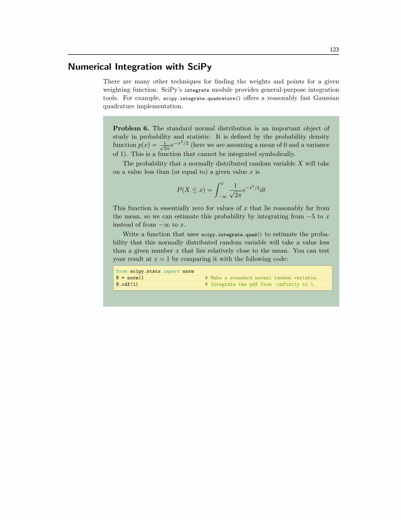
There are many other techniques for finding the weights and points for a givenweighting function. SciPy’s integrate module provides general-purpose integrationtools. For example, scipy.integrate.quadrature() o↵ers a reasonably fast Gaussianquadrature implementation.
Problem 6. The standard normal distribution is an important object ofstudy in probability and statistic. It is defined by the probability densityfunction p(x) = 1p
2⇡e�x
2/2 (here we are assuming a mean of 0 and a variance
of 1). This is a function that cannot be integrated symbolically.
The probability that a normally distributed random variable X will takeon a value less than (or equal to) a given value x is
P (X x) =
Zx
�1
1p2⇡
e�t
2/2dt
This function is essentially zero for values of x that lie reasonably far fromthe mean, so we can estimate this probability by integrating from �5 to xinstead of from �1 to x.
Write a function that uses scipy.integrate.quad() to estimate the proba-bility that this normally distributed random variable will take a value lessthan a given number x that lies relatively close to the mean. You can testyour result at x = 1 by comparing it with the following code:
from scipy.stats import norm
N = norm() # Make a standard normal random variable.
N.cdf(1) # Integrate the pdf from -infinity to 1.