Lab 0: Introduction to Networks lab - University of...
177
University of Jordan Faculty of Engineering & Technology Computer Engineering Department Computer Networks Laboratory 907528 Lab 0: Introduction to Networks lab
-
Upload
duonghuong -
Category
Documents
-
view
220 -
download
0
Transcript of Lab 0: Introduction to Networks lab - University of...
University of Jordan
Faculty of Engineering & Technology
Computer Engineering Department
Computer Networks Laboratory
907528
Lab 0: Introduction to Networks lab

1 Lab 0: Introduction to Networks lab
Introduction to Networking
By themselves, computers are powerful tools. When they are connected in a network, they
become even more powerful because the functions and tools that each computer provides can
be shared with other computers.
Network is a small group of computers that share information, or they can be very complex,
spanning large geographical areas that provide its users with unique capabilities, above and
beyond what the individual machines and their software applications can provide.
The goal of any computer network is to allow multiple computers to communicate. The type of
communication can be as varied as the type of conversations you might have throughout the
course of a day. For example, the communication might be a download of an MP3 audio file for
your MP3 player; using a web browser to check your instructor’s web page to see what
assignments and tests might be coming up; checking the latest sports scores; using an instant-
messaging service, such as Yahoo Messenger, to send text messages to a friend; or writing an e-
mail and sending it to a business associate.
Networks Advantages and Disadvantages:
-Network Hardware, Software and Setup Costs.-Hardware and Software Management & Administration Costs.-Undesirable Sharing.-Illegal or Undesirable Behavior.-Data Security Concerns.
-Connectivity and Communication.-Data SharingHardware Sharing.-Internet Access.-Data Security and Management.-Performance Enhancement and Balancing.-Entertainment.

2 Lab 0: Introduction to Networks lab
Network Types: Different types of networks are distinguished based on their size (in terms of the number of
machines), their data transfer speed, and their reach. There are usually said to be two categories
of networks:
Local Area Network (LAN)is limited to a specific area, usually an office, and cannot
extend beyond the boundaries of a single building. The first LANs were limited to a range
(from a central point to the most distant computer) of 185 meters (about 600 feet) and no more
than 30 computers. Today’s technology allows a larger LAN, but practical administration
limitations require dividing it into small, logical areas called workgroups.
A workgroup is a collection of individuals who share the same files and databases over the
LAN.
Wide Area Network (WAN)If you have ever connected to the Internet, you have used
the largest WAN on the planet. A WAN is any network that crosses metropolitan, regional, or
national boundaries. Most networking professionals define a WAN as any network that uses
routers and public network links. The Internet fits both definitions.

3 Lab 0: Introduction to Networks lab
The OSI and TCP/IP Networking Models: Models are useful because they help us understand difficult concepts and complicated systems.
When it comes to networking, there are several models that are used to explain the roles played
by various technologies, and how they interact. Of these, the most popular and commonly used
is the Open Systems Interconnection (OSI) Reference Model.
LAN WAN
Definition: LAN (Local Area Network) is a
computer network covering a
small geographic area, like a
home, office, schools, or group
of buildings.
WAN (Wide Area Network) is a
computer network that covers a
broad area or any network whose
communications links cross
metropolitan, regional, or national
boundaries over a long distance.
Speed: High speed(1000mbps) Less speed(150mbps)
Data transfer
rates:
High data transfer rate. Lower data transfer rate as
compared to LANs.
Example: Network in an organization. The Internet.
Components: Layer 2 devices like switches,
bridges. layer1 devices like
hubs , repeaters
Layers 3 devices Routers,
Switches and Technology specific
devices like ATM or Frame-relay
Switches.
Data Transmission
Error:
Experiences fewer data
transmission errors.
Experiences more data
transmission errors as compared to
LAN.
Ownership: Typically owned, controlled,
and managed by a single person
or organization.
WANs (like the Internet) are not
owned by any one organization
but rather exist under collective
distributed ownership and
management over long distances.
Set-up costs: Set-up an extra devices on the
network, it is not very
expensive.
Networks in remote areas have to
be connected, Set-up costs are
higher.
Maintenance costs: Covers a relatively small
geographical area, LAN is
easier to maintain at
relatively low costs.
Maintaining WAN is difficult
because of its wider geographical
coverage and higher maintenance
costs.
Geographical
Spread:
Have a
small geographical range.
Have a large geographical range
generally spreading across
boundaries.
Bandwidth: High bandwidth is available for
transmission.
Low bandwidth is available for
transmission.

4 Lab 0: Introduction to Networks lab
The OSI model was designed to promote interoperability by creating a guideline for network
data transmission between computers and components that have different hardware vendors,
software, operating systems, and protocols.
The idea behind the OSI Reference Model is to provide a framework for both designing
networking systems and for explaining how they work. The existence of the model makes it
easier for networks to be analyzed, designed, built and rearranged, by allowing them to be
considered as modular pieces that interact in predictable ways, rather than enormous, complex
monoliths.
TCP/IP Model
The Internet Protocol Suite, popularly known as the TCP/IP model, is a communication
protocol that is used over the Internet. This model divides the entire networking functions into
layers, where each layer performs a specific function.
This model gives a brief idea about the process of data formatting, transmission, and finally the
reception. Each of these functions takes place in the layers, as described by the model. TCP/IP
is a four-layered structure, with each layer having their individual protocol.
5 Lab 0: Introduction to Networks lab
Why Use a Layered Model?
By using a layered model, we can categorize the procedures that are necessary to transmit data
across a network. First, we need to define the term protocol: is a set of guidelines or rules of
communication.
Layered modeling allows us to:
• Create a protocol that can be designed and tested in stages, which, in turn, reduces the
complexity
• Enhance functionality of the protocol without adversely affecting the other layers
• Provide multivendor compatibility
• Allow for easier troubleshooting by locating the specific layer causing the problem
Both the TCP/IP and OSI model work in a very similar fashion. But they do have
very subtle differences too. The most apparent difference is the number of layers.
TCP/IP is a four-layered structure, while OSI is a seven-layered model.

6 Lab 0: Introduction to Networks lab
OSI model divides the network into seven layers and explains the routing of the data from
source to destination. It is a theoretical model which explains the working of the networks. Here
are the details of OSI's seven layers:
Application Layer (Layer 7)
The Application layer is a buffer between the user interface (what the user uses to perform
work) and the network application. This layer responsible for finding a communication partner
on the network. Once a partner is found, it is then responsible for ensuring that there is
sufficient network bandwidth to deliver the data.
This layer may also be responsible for synchronizing communication
and providing high level error checking between the two partners.
This ensures that the application is either sending or receiving, and
that the data transmitted is the same data received.
Typical applications include a client/server application (Telnet), an e-
mail application (SMTP), and an application to transfer files using
FTP or HTTP.
Presentation Layer (Layer 6)
The Presentation layer is responsible for the presentation of data to the Application layer. This
presentation may take the form of many structures. Data that it receives from the application
layer is converted into a suitable format that is recognized by the computer. Perform conversion
between ASCII and EBCDIC (a different character formatting method used on many
mainframes).
The Presentation layer must ensure that the application can view the appropriate data when it is
reassembled. Graphic files such as PICT, JPEG, TIFF, and GIF, and video and sound files such
as MPEG and Apple’s QuickTime are examples of Presentation layer responsibilities.
One final data structure is data encryption. Sometimes, it is vital that we can send data across a
network without someone being able to view our data, or snoop it.

7 Lab 0: Introduction to Networks lab
Session Layer (Layer 5)
The Session layer sets up and terminates communications between the two partners. Thislayer
decides on the method of communication: half-duplex or full-duplex.
Full-Duplex vs. Half-Duplex Communications
All network communications (including LAN and WAN communications) can be categorized
as Half-duplex or full-duplex. With half-duplex, communications happen in both directions, but
in only one direction at a time. When two computers communicate using half-duplex, one
computer sends a signal and the other receives; then, at some point, they switch sending and
receiving roles.
Full-duplex, on the other hand, allows communication in both directions simultaneously. Both
stations can send and receive signals at the same time. Full-duplex communications are similar
to a telephone call, in which both people can talk simultaneously.
8 Lab 0: Introduction to Networks lab
Transport Layer (Layer 4)
This layer provides end-to-end delivery of data between two nodes. It divides data into different
packets before transmitting it. On receipt of these packets, the data is reassembled and
forwarded to the next layer. If the data is lost in transmission or has errors, then this layer
recovers the lost data and transmits the same.
Transport layer add port number and sequence number to assemble and distinguish between
multiple applications segments received at a device; this also allows data to be multiplexed on
the line.
Multiplexing is the method of combining data from the upper layers and sending them through
the same data stream. This allows more than one application to communicate with the
communication partner at the same time. When the data reaches the remote partner, the
Transport layer then disassembles the segment and passes the correct data to each of the
receiving applications.
Network Layer (Layer 3)
The main function of this layer is routing data has to its intended destination on the network as
long as there is a physical network connection. The device that allows us to accomplish this
spectacular feat is the router, sometimes referred to as a Layer 3 device. While doing so, it has
to manage problems like network congestion, switching problems, etc.
In order for the router to succeed in this endeavor, it must be able to identify the source segment
and the final destination segment. This is done through network addresses, also called logical
addresses.
When a router receives data, it examines the Layer 3 data to determine the destination network
address. It then looks up the address in a table that tells it which route to use to get the data to
its final destination. It places the data on the proper connection, there by routing the packet
from one segment to another. The data may need to travel through many routers before
reaching its destination host. Each router in the path would perform the same lookup in its
table.

9 Lab 0: Introduction to Networks lab
Overview of IP Addresses
TCP/IP requires that each interface on a TCP/IP network have its own unique IP address. There
are two addressing schemes for TCP/IP: IPv4 and IPv6.
IPv4
An IPv4 address is a 32-bit number, usually represented as a four-part decimal number with
each of the four parts separated by a decimal point. In the IPv4 address, each individual byte, or
octet as it is sometimes called, can have a value in the range of 0 through 255.
The way these addresses are used varies according to the class of the network, so all you can
say with certainty is that the 32-bit IPv4 address is divided in some way to create an identifier
for the network, which all hosts on that network share, and an identifier for each host, which is
unique among all hosts on that network. In general, though, the higher-order bits of the address
make up the network part of the address and the rest constitutes the host part of the address. In
addition, the host part of the address can be divided further to allow for a sub network address.
IPv6
IPv6 was originally designed because the number of available unregistered IPv4 addresses was
running low. Because IPv6 uses a 128-bit addressing scheme, it has more than 79 octillion
times as many available addresses as IPv4. Also, instead of representing the binary digits as
decimal digits, IPv6 uses eight sets of four hexadecimal digits, like
so:3FFE:0B00:0800:0002:0000:0000:0000:000C.
Packets
At the Network layer, data coming from upper-layer protocols are divided into logical chunks
called packets. A packet is a unit of data transmission. The size and format of these packets
depend on the Network layer protocol in use. In other words, IP packets differ greatly from IPX
packets and Apple-Talk DDP packets, and the three are not compatible.

10 Lab 0: Introduction to Networks lab
Data Link Layer (Layer 2)
The main function of this layer is to convert the data packets received from the upper layer into
frames, and route the same to the physical layer. Error detection and correction is done at this
layer, thus making it a reliable layer in the model. It establishes a logical link between the nodes
and transmits frames sequentially.
The Data Link layer is split into two sub layers, the Logical Link Control (LLC) and the Media
Access Control (MAC). MAC sub layer is closer to the Physical layer.
The MAC sub layer defines a physical address, called a MAC address or hardware address,
which is unique to each individual network interface. This allows a way to uniquely identify
each network interface on a network, even if the network interfaces are on the same computer.
More importantly, though, the MAC address can be used in any network that supports the
chosen network interface.
11 Lab 0: Introduction to Networks lab
MAC layer on the receiving computer will take the bits from the Physical layer and put them in
order into a frame. It will also do a CRC (Cyclic Redundancy Check) to determine if there are
any errors in the frame.
It will check the destination hardware address to determine if the data is meant for it, or if it
should be dropped or sent on to the next machine. If the data is meant for the current computer,
it will pass it to the LLC layer.
The LLC layer is the buffer between the software protocols and the hardware protocols. It is
responsible for taking the data from the Network layer and sending it to the MAC layer. This
allows the software protocols to run on any type of network architecture.
What Is a MAC Address?
The MAC address is a unique value associated with a network adapter. MAC addresses
are also known as hardware addresses or physical addresses. They uniquely identify an
adapter on a LAN.
MAC addresses are 12-digit hexadecimal numbers (48 bits in length). By convention,
MAC addresses are usually written as the following format:
MM:MM:MM:SS:SS:SS or MM-MM-MM-SS-SS-SS
The first half of a MAC address contains the ID number of the adapter manufacturer.
These IDs are regulated by an Internet standards body (see sidebar). The second half of a
MAC address represents the serial number assigned to the adapter by the manufacturer.
MAC addresses function at the data link layer (layer 2). They allow computers to
uniquely identify themselves on a network at this relatively low level.

12 Lab 0: Introduction to Networks lab
Frames
At the Data Link layer, data coming from upper-layer protocols are divided into logical chunks
called frames. A frame is a unit of data transmission. The size and format of these frames
depend on the transmission technology. In other words, Ethernet frames differ greatly from
Token Ring frames and Frame Relay frames, and the three are not compatible.
Physical Layer (Layer 1)
As the name suggests, this is the layer where the physical connection between two computers
takes place. The data is transmitted via this physical medium to the destination's physical layer.
It is responsible for sending data and receiving data across a physical medium.
This data is sent in bits, either a 0 or a 1. The data may be transmitted as electrical signals (that
is, positive and negative voltages), audio tones, or light.
This layer also defines the Data Terminal Equipment (DTE) and the Data Circuit-Terminating
Equipment (DCE). The DTE is often accessed through a modem or a Channel Service
Unit/Data Service Unit (CSU/DSU) connected to a PC or a router. The carrier of the WAN
signal provides the DCE equipment. A typical device would be a packet switch, which is
responsible for clocking and switching.
Data Encapsulation Using the OSI Model
Since there may be more than one application using more than one communication partner
using more than one protocol, how does the data get to its destination correctly. This is
accomplished through a process called data encapsulation.

13 Lab 0: Introduction to Networks lab
Basically, it works like this:
1. A user is working on an application and decides to save the data to are mote server. The
application calls the Application layer to start the process.
2. The Application layer takes the data and places some information, called a header, at the
beginning. The header tells the Application layer which user application sent the data.
3. The Application layer then sends the data to the Presentation layer, where the data
conversion takes place. The Presentation layer places a header on all of the information
received from the Application layer (including the Application layer header). This header
identifies which protocol in the Application layer to pass it back.
4. The Presentation layer then sends the complete message to the Session layer. The Session
layer sets up the synchronized communication information to speak with the communication
partner and appends the information to another header.
5. The Session layer then sends the message to the Transport layer, where information is
placed into the header identifying the source and the destination hosts and the method of
connection (connectionless versus connection-oriented).
6. The Transport layer then passes the segment to the Network layer, where the network
address for the destination and the source are included in the header.
7. The Network layer passes the packet (connection-oriented) or the datagram
(connectionless) to the Data Link layer. The Data Link layer then includes the SSAP and the
DSAP to identify which Transport protocol to return it to. It also includes the source and the
destination MAC addresses.
14 Lab 0: Introduction to Networks lab
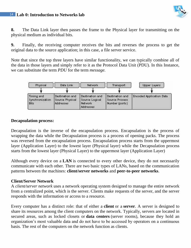
8. The Data Link layer then passes the frame to the Physical layer for transmitting on the
physical medium as individual bits.
9. Finally, the receiving computer receives the bits and reverses the process to get the
original data to the source application; in this case, a file server service.
Note that since the top three layers have similar functionality, we can typically combine all of
the data in those layers and simply refer to it as the Protocol Data Unit (PDU). In this Instance,
we can substitute the term PDU for the term message.
Decapsulation process:
Decapsulation is the inverse of the encapsulation process. Encapsulation is the process of
wrapping the data while the Decapsulation process is a process of opening packs. The process
was reversed from the encapsulation process. Encapsulation process starts from the uppermost
layer (Application Layer) to the lowest layer (Physical layer) while the Decapsulation process
starts from the lowest layer (Physical Layer) to the uppermost layer (Application Layer)
Although every device on a LAN is connected to every other device, they do not necessarily
communicate with each other. There are two basic types of LANs, based on the communication
patterns between the machines: client/server networks and peer-to-peer networks.
Client/Server Network
A client/server network uses a network operating system designed to manage the entire network
from a centralized point, which is the server. Clients make requests of the server, and the server
responds with the information or access to a resource.
Every computer has a distinct role: that of either a client or a server. A server is designed to
share its resources among the client computers on the network. Typically, servers are located in
secured areas, such as locked closets or data centers (server rooms), because they hold an
organization’s most valuable data and do not have to be accessed by operators on a continuous
basis. The rest of the computers on the network function as clients.

15 Lab 0: Introduction to Networks lab
Peer-to-Peer Network
In peer-to-peer networks, the connected computers have no centralized authority. From an
authority viewpoint, all of these computers are equal. In other words, they are peers. If a user of
one computer wants access to a resource on another computer, the security check for access
rights is the responsibility of the computer holding the resource.
Each computer in a peer-to-peer network can be both a client that requests resources and a
server that provides resources.
Application Layer Services and Protocols
Understanding Servers In the truest sense, a server does exactly what the name implies: It provides resources to the
clients on the network (“serves” them, in other words). Servers are typically powerful
computers that run the software that controls and maintains.
16 Lab 0: Introduction to Networks lab
Servers are often specialized for a single purpose. This is not to say that a single server can’t do
many jobs, but you’ll get better performance if you dedicate a server to a single task. Here are
some examples of servers that are dedicated to a single task:
File Server Holds and distributes files.
Print Server Controls and manages one or more printers for the network.
Proxy Server Performs a function on behalf of other computers.
Application Server Hosts a network application.
Web Server Holds and delivers web pages and other web content using the Hypertext
Transfer Protocol (HTTP).
Mail Server Hosts and delivers e-mail. It’s the electronic equivalent of a post office.
Fax Server Sends and receives faxes for the entire network without the need for paper.
Telephony Server Functions as a “smart” answering machine for the network. It can
also perform call center and call-routing functions.
Notice that each server type’s name consists of the type of service the server provides
(remote access, for example) followed by the word server, which, as you remember, means to
serve.
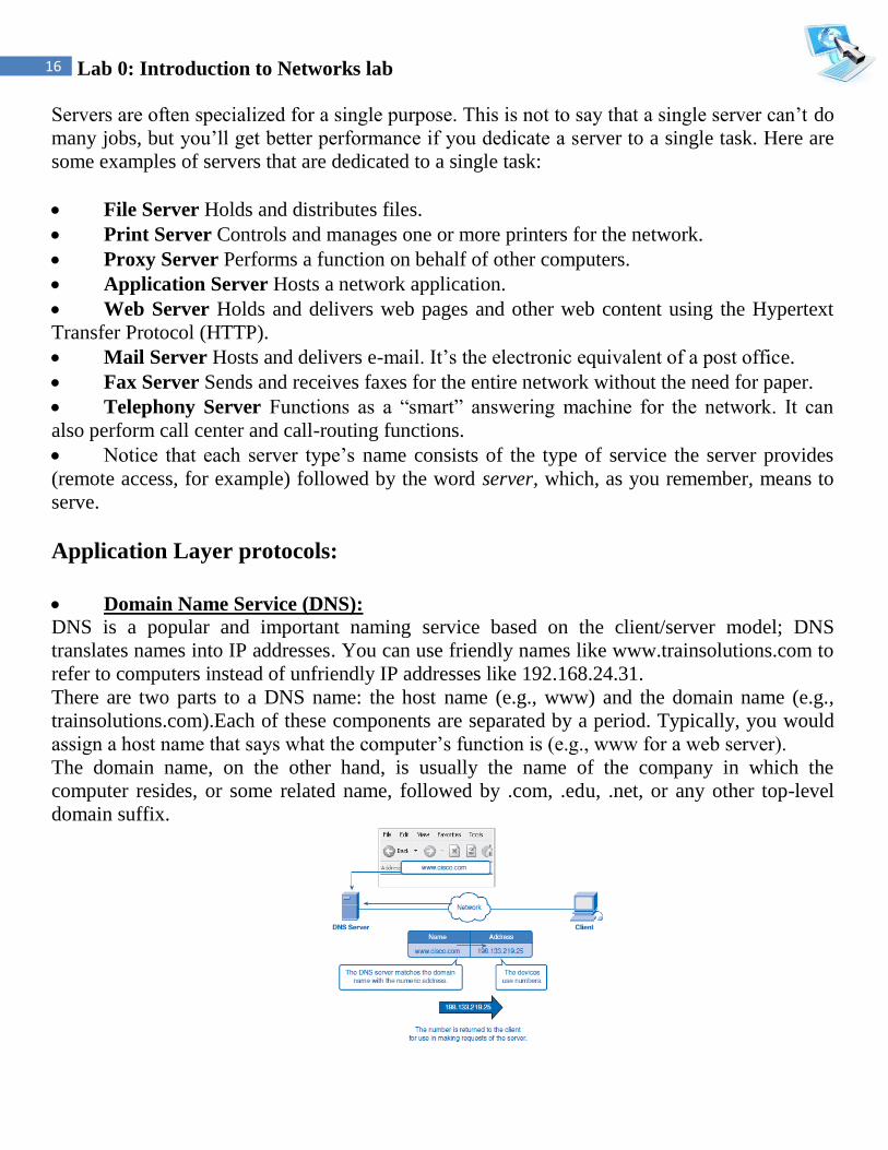
Application Layer protocols: Domain Name Service (DNS): DNS is a popular and important naming service based on the client/server model; DNS
translates names into IP addresses. You can use friendly names like www.trainsolutions.com to
refer to computers instead of unfriendly IP addresses like 192.168.24.31.
There are two parts to a DNS name: the host name (e.g., www) and the domain name (e.g.,
trainsolutions.com).Each of these components are separated by a period. Typically, you would
assign a host name that says what the computer’s function is (e.g., www for a web server).
The domain name, on the other hand, is usually the name of the company in which the
computer resides, or some related name, followed by .com, .edu, .net, or any other top-level
domain suffix.

17 Lab 0: Introduction to Networks lab
Dynamic Host Configuration Protocol (DHCP):
DHCP used to provide IP configuration information to hosts on boot up. DHCP manages
addressing by leasing the IP information to the hosts. This leasing allows the information to be
recovered when not in use and reallocated when needed.
The primary reason for using DHCP is to centralize the management of IP addresses. When the
DHCP service is used, DHCP scopes include pools of IP addresses that are assigned for
automatic distribution to client computers on an as-needed basis, in the form of leases, which
are periods of time for which the DHCP client may keep the configuration assignment. Clients
attempt to renew their lease at 50 percent of the lease duration. The address pools are
centralized on the DHCP server, allowing all IP addresses on your network to be administered
from a single server.
It should be apparent that this saves loads of time when changing the IP addresses on your
network. Instead of running around to every workstation and server and resetting the IP address
to a new address, you simply reset the IP address pool on the DHCP server. The next time the
client machines are rebooted, they are assigned new addresses.
DHCP Information can include:
• IP address.
• Subnet mask.
• Default gateway.
• Domain name.
• DNS Server.
Simple Network Management Protocol (SNMP):
SNMP allows network administrators to collect information about the network. It is a
communications protocol for collecting information about devices on the network, including
hubs, routers, and bridges. Each piece of information to be collected about a device is defined
in a Management Information Base (MIB). SNMP uses UDP to send and receive messages on
the network.
18 Lab 0: Introduction to Networks lab
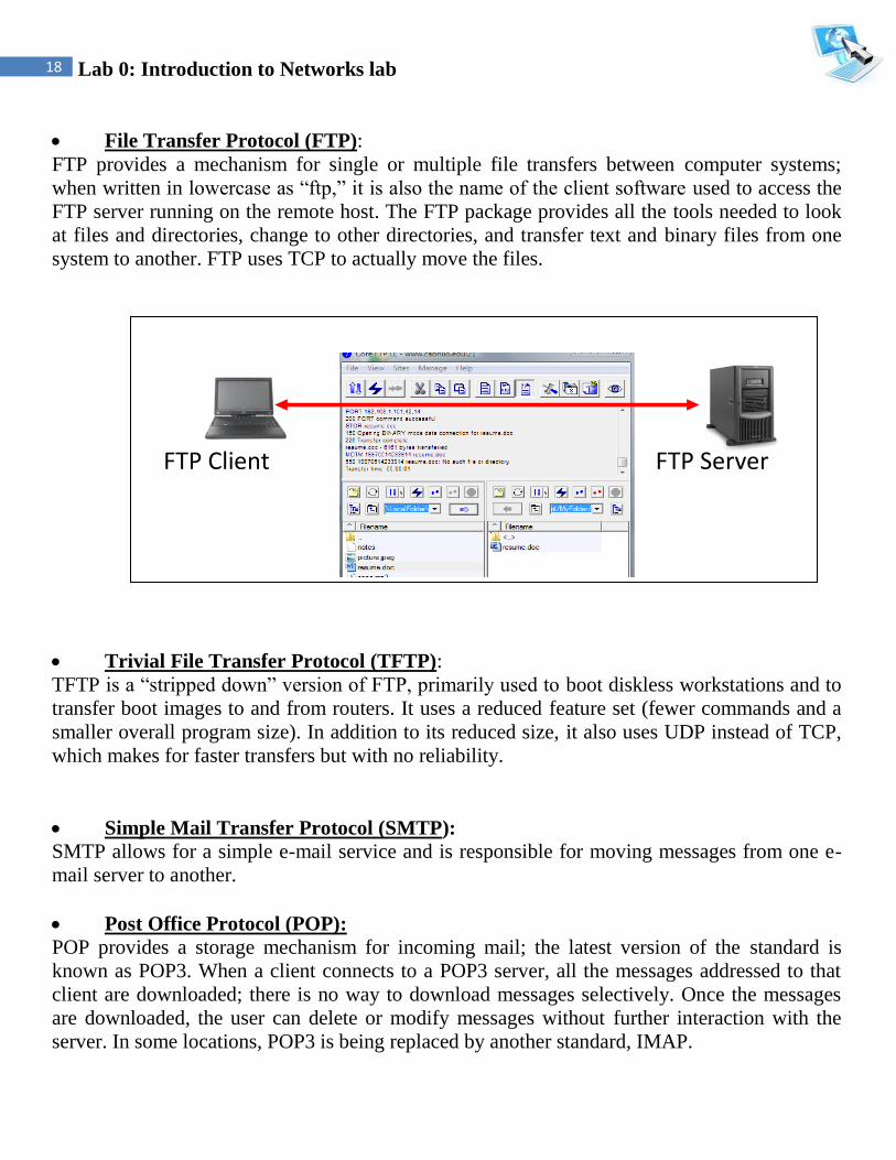
File Transfer Protocol (FTP):
FTP provides a mechanism for single or multiple file transfers between computer systems;
when written in lowercase as “ftp,” it is also the name of the client software used to access the
FTP server running on the remote host. The FTP package provides all the tools needed to look
at files and directories, change to other directories, and transfer text and binary files from one
system to another. FTP uses TCP to actually move the files.
Trivial File Transfer Protocol (TFTP):
TFTP is a “stripped down” version of FTP, primarily used to boot diskless workstations and to
transfer boot images to and from routers. It uses a reduced feature set (fewer commands and a
smaller overall program size). In addition to its reduced size, it also uses UDP instead of TCP,
which makes for faster transfers but with no reliability.
Simple Mail Transfer Protocol (SMTP):
SMTP allows for a simple e-mail service and is responsible for moving messages from one e-
mail server to another.
Post Office Protocol (POP):
POP provides a storage mechanism for incoming mail; the latest version of the standard is
known as POP3. When a client connects to a POP3 server, all the messages addressed to that
client are downloaded; there is no way to download messages selectively. Once the messages
are downloaded, the user can delete or modify messages without further interaction with the
server. In some locations, POP3 is being replaced by another standard, IMAP.
FTP Client
FTP Server
FTP Client FTP Server

19 Lab 0: Introduction to Networks lab
Telnet
Telnet is a terminal emulation protocol that provides a remote logon to another host over the
network. It allows a user to connect to a remote host over a TCP/IP connection as if they were
sitting right at that host. Keystrokes typed into a Telnet program will be transmitted over a
TCP/IP network to the host. The visual responses are sent back by the host to the Telnet client
to be displayed.
20 Lab 0: Introduction to Networks lab
Secure Shell (SSH):
SSH used to establish a secure Telnet session over a standard TCP/ IP connection. It is used to
run programs on remote systems, log in to other systems, and move files from one system to
another, all while maintaining a strong, encrypted connection.
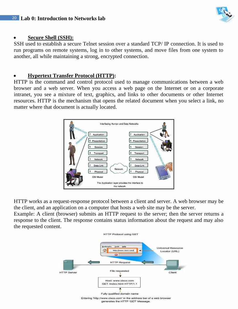
Hypertext Transfer Protocol (HTTP):
HTTP is the command and control protocol used to manage communications between a web
browser and a web server. When you access a web page on the Internet or on a corporate
intranet, you see a mixture of text, graphics, and links to other documents or other Internet
resources. HTTP is the mechanism that opens the related document when you select a link, no
matter where that document is actually located.
HTTP works as a request-response protocol between a client and server. A web browser may be
the client, and an application on a computer that hosts a web site may be the server.
Example: A client (browser) submits an HTTP request to the server; then the server returns a
response to the client. The response contains status information about the request and may also
the requested content.

21 Lab 0: Introduction to Networks lab
Two HTTP Request Methods: GET and POST
Two commonly used methods for a request-response between a client and server are: GET and
POST.
GET - Requests data from a specified resource. Its header consists of many parameters.
POST - Submits data to be processed to a specified resource
Hypertext Transfer Protocol Secure (HTTPS) HTTPS is a secure version of HTTP that provides a variety of security mechanisms to the
transactions between a web browser and the server. HTTPS allows browsers and servers to
sign, authenticate, and encrypt an HTTP message.

22 Lab 0: Introduction to Networks lab
Transport layer protocols (TCP/UDP)
TCP stands for Transmission Control Protocol, and UDP is the abbreviation for User Datagram
Protocol. Both pertain to data transmissions on the Internet, but they work very differently.
TCP UDP
Acronym for: Transmission Control Protocol User Datagram Protocol
Function: As a message makes its way
across the internet from one
computer to another. This is
connection based.
UDP is also a protocol used in
message transport or transfer. This is
not connection based.
Usage: TCP is used in case of non-time
critical applications.
UDP is used for games or applications
that require fast transmission of data.
Examples: HTTP, HTTPs, FTP, SMTP
Telnet etc...
DNS, DHCP, TFTP, SNMP, RIP,
VOIP etc...
Ordering of data
packets:
TCP rearranges data packets
in the order specified.
UDP has no order as all packets are
independent of each other. If ordering
is required, it has to be managed by
the application layer.
Speed of transfer: The speed for TCP is slower than
UDP.
UDP is faster because there is no
error-checking for packets.
Reliability: There is absolute guarantee that
the data transferred remains
intact and arrives in the same
order in which it was sent.
There is no guarantee that the
messages or packets sent would reach
at all.
Header Size: TCP header size is 20 bytes UDP Header size is 8 bytes.
Streaming of data: Data is read as a byte stream,
no indications are transmitted to
signal message(segment)
boundaries.
Packets sent and checked individually
for integrity only if they arrive.
Packets have definite boundaries
which are honored uponreceipt.
Data Flow Control: TCP does Flow Control, handles
reliability and congestion
control.
UDP does not have an option forflow
control
Error Checking: TCP does error checking UDP does error checking, but no
recovery options.
Acknowledgement: Acknowledgement segments No Acknowledgment

23 Lab 0: Introduction to Networks lab
Port number
A port number is a way to identify a specific process to which an Internet or other network
message is to be forwarded when it arrives at a server. For the Transmission Control Protocol
and the User Datagram Protocol, a port number is a 16-bit integer that is put in the header
appended to a message unit. This port number is passed logically between client and server
transport layers and physically between the transport layer and the Internet Protocol layer and
forwarded on.
For example, a request from a client (perhaps on behalf of you at your PC) to a server on the
Internet may request a file be served from that host's File Transfer Protocol (FTP) server or
process. In order to pass your request to the FTP process in the remote server, the Transmission
Control Protocol (TCP) software layer in your computer identifies the port number of 21
(which by convention is associated with an FTP request) in the 16-bit port number integer that
is appended to your request. At the server, the TCP layer will read the port number of 21 and
forward your request to the FTP program at the server.
Port Range Groups
0 to 1023 - Well known port numbers: Reserved for common services and applications.
1024 to 49151 - Registered ports; meaning they can be registered to specific protocols
by software corporations.
49152 to 65536 - Dynamic or private ports; usually assigned dynamically to client
applications initiating a connection.
Port
Number
Application Layer 4
Protocol
Description
20 FTP TCP File Transfer Protocol – Data
21 FTP TCP File Transfer Protocol – Control Commands
23 TELNET TCP Terminal connection
25 SMTP TCP Simple Mail Transfer Protocol - Email
53 DNS UDP Domain Name System
67,68 DHCP UDP Dynamic Host Configuration Protocol
69 TFTP UDP Trivial File Transfer Protocol
80 HTTP TCP Hypertext Transfer Protocol

24 Lab 0: Introduction to Networks lab
Commutation message types:
Unicast
Unicast packets are sent from host to host. The communication is from a single host to another
single host. There is one device transmitting a message destined for one receiver.
Broadcast
Broadcast is when a single device is transmitting a message to all other devices in a given
address range. This broadcast could reach all hosts on the subnet, all subnets, or all hosts on all
subnets. Broadcast packets have the host (and/or subnet) portion of the address set to all ones.
By design, most modern routers will block IP broadcast traffic and restrict it to the local subnet.
Multicast
Multicast is a special protocol for use with IP. Multicast enables a single device to
communicate with a specific set of hosts, not defined by any standard IP address and mask
combination. This allows for communication that resembles a conference call. Anyone from
anywhere can join the conference, and everyone at the conference hears what the speaker has to
say. The speaker's message isn't broadcasted everywhere, but only to those in the conference
call itself. A special set of addresses is used for multicast communication.

25 Lab 0: Introduction to Networks lab
To configure TCP/IP settings:
1. Open Network Connections
2. Click the connection you want to configure, and then, under Network Tasks,
click Change settings of this connection.
3. Do one of the following:
• If the connection is a local area connection, on the General tab, under This
connection uses the following items, click Internet Protocol (TCP/IP), and then
click Properties.
• If this is a dial-up, VPN, or incoming connection, click the Networking tab. In This
connection uses the following items, click Internet Protocol (TCP/IP), and then
click Properties.
4. Do one of the following:
• If you want IP settings to be assigned automatically, click Obtain an IP address
automatically, and then click OK.
• If you want to specify an IP address or a DNS server address, do the following:
• Click Use the following IP address, and in IP address, type the IP address.
• Click Use the following DNS server addresses, and in Preferred DNS
server and Alternate DNS server, type the addresses of the primary and
secondary DNS servers.
5. To configure DNS, WINS, and IP Settings, click Advanced.

University of Jordan
Faculty of Engineering & Technology
Computer Engineering Department
Computer Networks Laboratory
907528
Lab1: Cabling & Packet Sniffing

1 Lab1: Cabling & Packet Sniffing
Physical media refers to the physical materials that are used to transmit information in data
communications. It is referred to as physical media because the media is generally a
physical object such as copper or glass.
Although it is possible to use several forms of wireless networking, such as radio frequency
and Infrared, the majority of installed LANs today communicate via some sort of cable. In
the following sections, we’ll look at two types of cables:
Twisted pair.
Fiber optic.
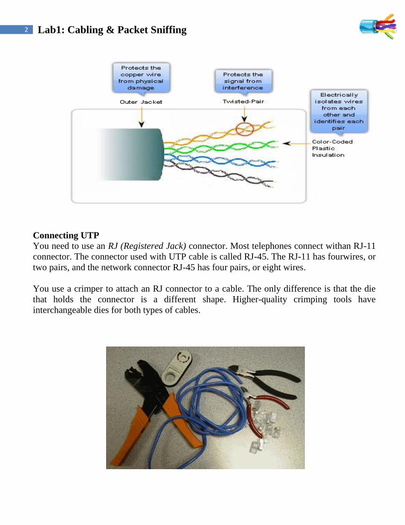
Twisted-Pair Cable
Twisted-pair cable consists of multiple, individually insulated wires that are twisted
together in pairs. Sometimes a metallic shield is placed around the twisted pairs. Hence, the
name shielded twisted-pair (STP).
Also you will see cable without outer shielding; it’s called unshielded twisted-pair (UTP).
UTP is commonly used in twisted-pair Ethernet (10Base-T, 100Base-TX, etc.), star-wired
networks.
Let’s take a look at why the wires in this cable type are twisted. When electromagnetic
signals are conducted on copper wires that are in close proximity (such as inside a cable),
some electromagnetic interference occurs. In this scenario, this interference is called
crosstalk. Twisting two wires together as a pair minimizes such interference and also
provides some protection against interference from outside sources.
2 Lab1: Cabling & Packet Sniffing
Connecting UTP You need to use an RJ (Registered Jack) connector. Most telephones connect withan RJ-11
connector. The connector used with UTP cable is called RJ-45. The RJ-11 has fourwires, or
two pairs, and the network connector RJ-45 has four pairs, or eight wires.
You use a crimper to attach an RJ connector to a cable. The only difference is that the die
that holds the connector is a different shape. Higher-quality crimping tools have
interchangeable dies for both types of cables.

3 Lab1: Cabling & Packet Sniffing
Types of Interfaces
In an Ethernet LAN, devices use one of two types of UTP interfaces - MDI or MDIX.
The MDI (media-dependent interface) uses the normal Ethernet pinouts. Pins 1 and 2 are
used for transmitting and pins 3 and 6 are used for receiving. Devices such as computers,
servers, or routers will have MDI connections.
The devices that provide LAN connectivity - usually hubs or switches - typically use MDIX
(media-dependent interface, crossover) connections. The MDIX connection swaps the
transmit pairs internally. This swapping allows the end devices to be connected to the hub
or switch using a straight-through cable.
Typically, when connecting different types of devices, use a straight-through cable. And
when connecting the same type of device, use a crossover cable.
UTP Cables Connections types:
Straight-through UTP Cables
A straight-through cable has connectors on each end that are terminated the same in
accordance with either the T568A or T568B standards.
Identifying the cable standard used allows you to determine if you have the right cable for
the job. More importantly, it is a common practice to use the same color codes throughout
the LAN for consistency in documentation.
Use straight-through cables for the following connections:
Switch to a router Ethernet port
Computer to switch
Computer to hub
Crossover UTP Cables
For two devices to communicate through a cable that is directly connected between the two,
the transmit terminal of one device needs to be connected to the receive terminal of the
other device.
The cable must be terminated so the transmit pin, Tx, taking the signal from device A at one
end, is wired to the receive pin, Rx, on device B. Similarly, device B's Tx pin must be
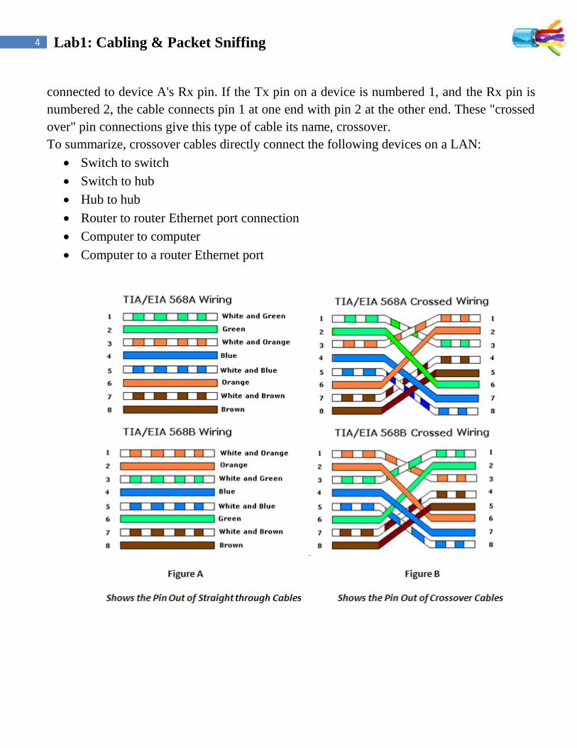
4 Lab1: Cabling & Packet Sniffing
connected to device A's Rx pin. If the Tx pin on a device is numbered 1, and the Rx pin is
numbered 2, the cable connects pin 1 at one end with pin 2 at the other end. These "crossed
over" pin connections give this type of cable its name, crossover.
To summarize, crossover cables directly connect the following devices on a LAN:
Switch to switch
Switch to hub
Hub to hub
Router to router Ethernet port connection
Computer to computer
Computer to a router Ethernet port

5 Lab1: Cabling & Packet Sniffing
Rollover UTP Cables
In a rolled cable, the colored wires at one end of the cable are in the reverse sequence of the
colored wires at the other end of the cable.
Console Cables (RJ-45 to DB-9 Female)
This cable is also known as Management Cable.
The connection to the console is made by plugging the DB-9 connector into an available
EIA/TIA 232 serial port on the computer. It is important to remember that if there is more
than one serial port, note which port number is being used for the console connection. Once
the serial connection to the computer is made, connect the RJ-45 end of the cable directly
into the console interface on the router.

6 Lab1: Cabling & Packet Sniffing
Fiber-Optic Cable
Fiber-optic cable transmits digital signals using light impulses rather than electricity; it is
immune to Electromagnetic Interference (EMI) and Radio Frequency Interference (RFI).
Light is carried on either a glass or a plastic core. Glass can carry the signal a greater
distance, but plastic costs less. Regardless of which core is used, the core is surrounded by a
glass or plastic cladding, which is more glass or plastic with a different index of refraction
that refracts the light back into the core. Around this is a layer of flexible plastic buffer.
This can be then wrapped in an armor coating and then sheathed in PVC or plenum.

7 Lab1: Cabling & Packet Sniffing
The cable itself comes in two different styles: single-mode fiber (SMF) and multimode fiber
(MMF).
Single mode fiber optic:
Glass core 8 – 10 micrometers diameter.
Laser light source produces single ray of light.
Distances up to 100km.
Photodiodes to convert light back to electrical signals.
Multimode fiber optic:
Glass core 50 – 60 micrometers diameter.
LED light source produces many rays of light at
different angles, travel at different speeds.
Distances up to 2km, limited by dispersion.
Photodiode receptors.
Cheaper than single mode.
Although fiber-optic cable may sound like the solution to many problems:
Is completely immune to EMI or RFI
Can transmit up to 40 kilometers (about 25 miles)
Here are the Problems of fiber-optic cable:
Is difficult to install
Requires a bigger investment in installation and materials.
Serial Cables In the lab experiments, you may be using Cisco routers with one of two types of physical
serial cables. Both cables use a large Winchester 15 Pin connector on the network end. This
end of the cable is used as a V.35 connection to a Physical layer device such as a
CSU/DSU.
The first cable type has a male DB-60 connector on the Cisco end and a male Winchester
connector on the network end. The second type is a more compact version of this cable and
has a Smart Serial connector on the Cisco device end. It is necessary to be able to identify
the two different types in order to connect successfully to the router.

8 Lab1: Cabling & Packet Sniffing
Data Communications Equipment and Data Terminal Equipment
The following terms describe the types of devices that maintain the link between a sending
and a receiving device:
Data Communications Equipment (DCE) - A device that supplies the clocking services to
another device. Typically, this device is at the WAN access provider end of the link.
Data Terminal Equipment (DTE) - A device that receives clocking services from another
device and adjusts accordingly. Typically, this device is at the WAN customer or user end
of the link.
If a serial connection is made directly to a service provider or to a device that provides
signal clocking such as a channel service unit/data service unit (CSU/DSU), the router is
considered to be data terminal equipment (DTE) and will use a DTE serial cable.
DCEs and DTEs are used in WAN connections. The communication via a WAN connection
is maintained by providing a clock rate that is acceptable to both the sending and the
receiving device. In most cases, the ISP provides the clocking service that synchronizes the
transmitted signal.

9 Lab1: Cabling & Packet Sniffing
When making WAN connections between two routers in a lab, connect two routers with a
serial cable to simulate a point-to-point WAN link. In this case, decide which router is
going to be the one in control of clocking. Routers are DTE devices by default, but they can
be configured to act as DCE devices.
The V35 compliant cables are available in DTE and DCE versions. To create a point-to-
point serial connection between two routers, join together a DTE and DCE cable. Each
cable comes with connectors that mate with its complementary type. These connectors are
configured so that you cannot join two DCE or two DTE cables together by mistake.
10 Lab1: Cabling & Packet Sniffing
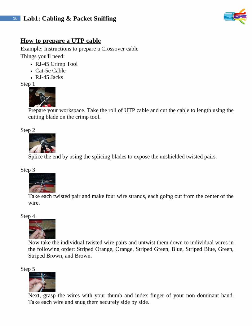
How to prepare a UTP cable
Example: Instructions to prepare a Crossover cable
Things you'll need:
RJ-45 Crimp Tool
Cat-5e Cable
RJ-45 Jacks
Step 1
Prepare your workspace. Take the roll of UTP cable and cut the cable to length using the
cutting blade on the crimp tool.
Step 2
Splice the end by using the splicing blades to expose the unshielded twisted pairs.
Step 3
Take each twisted pair and make four wire strands, each going out from the center of the
wire.
Step 4
Now take the individual twisted wire pairs and untwist them down to individual wires in
the following order: Striped Orange, Orange, Striped Green, Blue, Striped Blue, Green,
Striped Brown, and Brown.
Step 5
Next, grasp the wires with your thumb and index finger of your non-dominant hand.
Take each wire and snug them securely side by side.

11 Lab1: Cabling & Packet Sniffing
Step 6
Using the cutting blade of the crimp tool, cut the ends off of the wires to make each wire
the same height.
Step 7
Still grasping the wires, insert the RJ-45 jack on the wires with the clip facing away
from you.
Step 8
Insert the jack into the crimper and press down tightly on the tool to seal the wires in
place.
Step 9
Once the first head is made, repeat steps two through eight. When untwisting the wires
down to sing strands, use the following order: Striped Green, Green, Striped Orange,
Blue, Striped Blue, Orange, Striped Brown, Brown.
Step 10
Plug in the cable to test connectivity.
12 Lab1: Cabling & Packet Sniffing
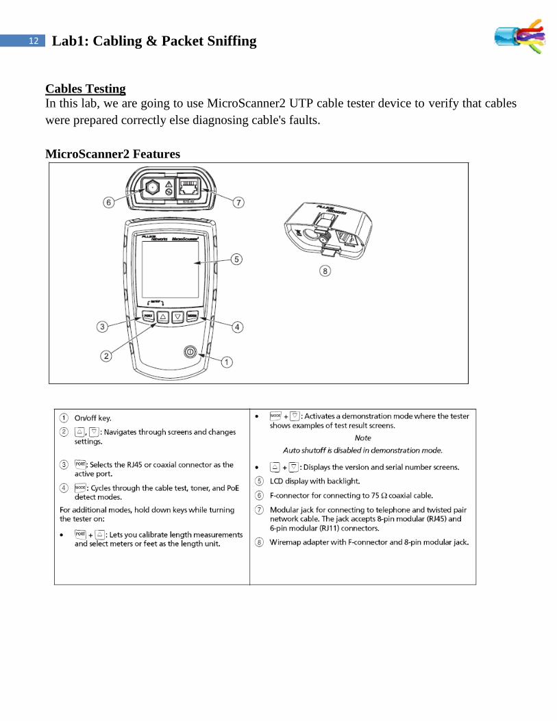
Cables Testing
In this lab, we are going to use MicroScanner2 UTP cable tester device to verify that cables
were prepared correctly else diagnosing cable's faults.
MicroScanner2 Features

13 Lab1: Cabling & Packet Sniffing
Auto Shutoff
The tester turns off after 10 minutes if no keys are pressed and nothing changes at the
tester’s connectors.
Changing the Length Units

14 Lab1: Cabling & Packet Sniffing
15 Lab1: Cabling & Packet Sniffing

16 Lab1: Cabling & Packet Sniffing
Diagnosing Wire map Faults
Open
• Wires connected to wrong pins at connector or punch down blocks
• Faulty connections
• Damaged connector
• Damaged cable
• Wrong pairs selected in setup
• Wrong application for cable

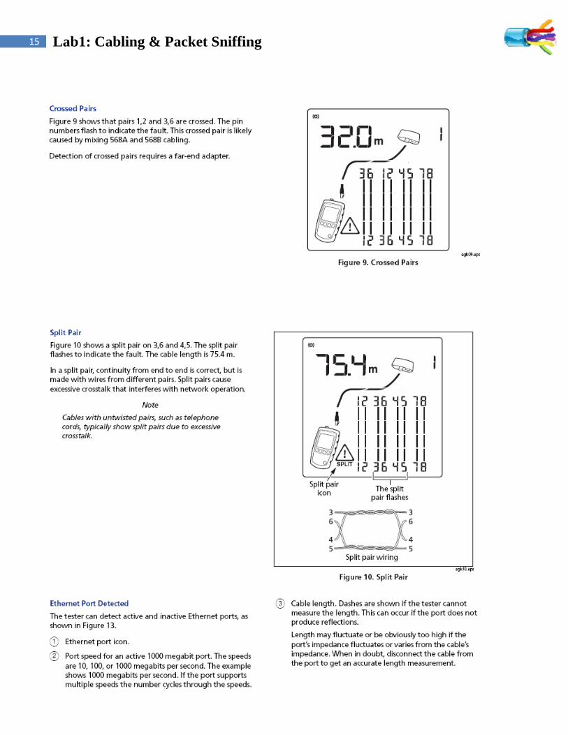
17 Lab1: Cabling & Packet Sniffing
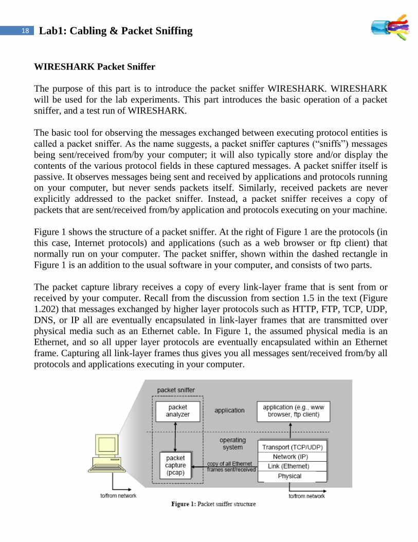
Split Pair
Wires connected to wrong pins at connector or punch down block.
Reversed Pairs
Wires connected to wrong pins at connector or punch down block.
Crossed Pairs
• Wires connected to wrong pins at connector or punch down block.
• Mix of 568A and 568B wiring standards (12 and 36 crossed).
• Crossover cables used where not needed (12 and 36 crossed).
Short
• Damaged connector
• Damaged cable
• Conductive material stuck between pins at connector.
• Improper connector termination
• Wrong application for cable
18 Lab1: Cabling & Packet Sniffing
WIRESHARK Packet Sniffer
The purpose of this part is to introduce the packet sniffer WIRESHARK. WIRESHARK
will be used for the lab experiments. This part introduces the basic operation of a packet
sniffer, and a test run of WIRESHARK.
The basic tool for observing the messages exchanged between executing protocol entities is
called a packet sniffer. As the name suggests, a packet sniffer captures (“sniffs”) messages
being sent/received from/by your computer; it will also typically store and/or display the
contents of the various protocol fields in these captured messages. A packet sniffer itself is
passive. It observes messages being sent and received by applications and protocols running
on your computer, but never sends packets itself. Similarly, received packets are never
explicitly addressed to the packet sniffer. Instead, a packet sniffer receives a copy of
packets that are sent/received from/by application and protocols executing on your machine.
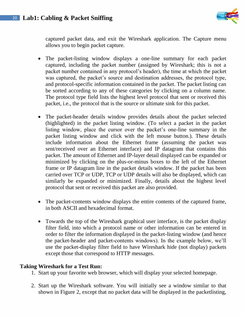
Figure 1 shows the structure of a packet sniffer. At the right of Figure 1 are the protocols (in
this case, Internet protocols) and applications (such as a web browser or ftp client) that
normally run on your computer. The packet sniffer, shown within the dashed rectangle in
Figure 1 is an addition to the usual software in your computer, and consists of two parts.
The packet capture library receives a copy of every link-layer frame that is sent from or
received by your computer. Recall from the discussion from section 1.5 in the text (Figure
1.202) that messages exchanged by higher layer protocols such as HTTP, FTP, TCP, UDP,
DNS, or IP all are eventually encapsulated in link-layer frames that are transmitted over
physical media such as an Ethernet cable. In Figure 1, the assumed physical media is an
Ethernet, and so all upper layer protocols are eventually encapsulated within an Ethernet
frame. Capturing all link-layer frames thus gives you all messages sent/received from/by all
protocols and applications executing in your computer.

19 Lab1: Cabling & Packet Sniffing
The second component of a packet sniffer is the packet analyzer, which displays the
contents of all fields within a protocol message. In order to do so, the packet analyzer must
“understand” the structure of all messages exchanged by protocols. For example, suppose
we are interested in displaying the various fields in messages exchanged by the HTTP
protocol in Figure 1. The packet analyzer understands the format of Ethernet frames, and so
can identify the IP datagram within an Ethernet frame. It also understands the IP datagram
format, so that it can extract the TCP segment within the IP datagram.
Finally, it understands the TCP segment structure, so it can extract the HTTP message
contained in the TCP segment. Finally, it understands the HTTP protocol and so, for
example, knows that the first bytes of an HTTP message will contain the string “GET,”
“POST,” or “HEAD
Running Wireshark
When you run the Wireshark program, the Wireshark graphical user interface shown in
Figure 2 will be displayed. Initially, no data will be displayed in the various windows.
The Wireshark interface has five major components:
The command menus are standard pull-down menus located at the top of the
window. Of interest to us now is the File and Capture menus. The File menu
allows you to save captured packet data or open a file containing previously
20 Lab1: Cabling & Packet Sniffing
captured packet data, and exit the Wireshark application. The Capture menu
allows you to begin packet capture.
The packet-listing window displays a one-line summary for each packet
captured, including the packet number (assigned by Wireshark; this is not a
packet number contained in any protocol’s header), the time at which the packet
was captured, the packet’s source and destination addresses, the protocol type,
and protocol-specific information contained in the packet. The packet listing can
be sorted according to any of these categories by clicking on a column name.
The protocol type field lists the highest level protocol that sent or received this
packet, i.e., the protocol that is the source or ultimate sink for this packet.
The packet-header details window provides details about the packet selected
(highlighted) in the packet listing window. (To select a packet in the packet
listing window, place the cursor over the packet’s one-line summary in the
packet listing window and click with the left mouse button.). These details
include information about the Ethernet frame (assuming the packet was
sent/received over an Ethernet interface) and IP datagram that contains this
packet. The amount of Ethernet and IP-layer detail displayed can be expanded or
minimized by clicking on the plus-or-minus boxes to the left of the Ethernet
frame or IP datagram line in the packet details window. If the packet has been
carried over TCP or UDP, TCP or UDP details will also be displayed, which can
similarly be expanded or minimized. Finally, details about the highest level
protocol that sent or received this packet are also provided.
The packet-contents window displays the entire contents of the captured frame,
in both ASCII and hexadecimal format.
Towards the top of the Wireshark graphical user interface, is the packet display
filter field, into which a protocol name or other information can be entered in
order to filter the information displayed in the packet-listing window (and hence
the packet-header and packet-contents windows). In the example below, we’ll
use the packet-display filter field to have Wireshark hide (not display) packets
except those that correspond to HTTP messages.
Taking Wireshark for a Test Run:
1. Start up your favorite web browser, which will display your selected homepage.
2. Start up the Wireshark software. You will initially see a window similar to that
shown in Figure 2, except that no packet data will be displayed in the packetlisting,

21 Lab1: Cabling & Packet Sniffing
packet-header, or packet-contents window, since Wireshark has not yet begun
capturing packets.
3. To begin packet capture, select the Capture pull down menu and select Options.
This will cause the “Wireshark: Capture Options” window to be displayed, as
shown in Figure 3.
4. You can use most of the default values in this window, but uncheck “Hide capture
info dialog” under Display Options. The networks interface (i.e., the physical
connections) that your computer has to the network will be shown in the Interface
pull down menu at the top of the Capture Options window. In case your computer
has more than one active network interface (e.g., if you have both a wireless and a
wired Ethernet connection), you will need to select an interface that is being used to
send and receive packets (mostly likely the wired interface). After selecting the
network interface (or using the default interface chosen by Wireshark), click Start.
Packet capture will now begin - all packets being sent/received from/by your
computer are now being captured by Wireshark!

22 Lab1: Cabling & Packet Sniffing
5. Once you begin packet capture, a packet capture summary window will appear, as
shown in Figure 4. This window summarizes the number of packets of various
types that are being captured, and (importantly!) contains the Stop button that will
allow you to stop packet capture. Don’t stop packet capture yet.
6. While Wireshark is running, enter the URL:
http://gaia.cs.umass.edu/wireshark-labs/INTRO-wireshark-file1.html
And have that page displayed in your browser. In order to display this page, your
browser will contact the HTTP server at gaia.cs.umass.edu and exchange HTTP
messages with the server in order to download this page. The Ethernet frames
containing these HTTP messages will be captured by Wireshark.
7. After your browser has displayed the INTRO-wireshark-file1.html page, stop
Wireshark packet capture by selecting stop in the Wireshark capture window.
This will cause the Wireshark capture window to disappear and the main Wireshark
window to display all packets captured since you began packet capture.
The main Wireshark window should now look similar to Figure 2. You now have
live packet data that contains all protocol messages exchanged between your
computer and other network entities! The HTTP message exchanges with the
gaia.cs.umass.edu web server should appear somewhere in the listing of packets
captured. But there will be many other types of packets displayed as well (see, e.g.,
the many different protocol types shown in the Protocol column in Figure 2).
8. Type in “http” (without the quotes, and in lower case – all protocol names are in
lower case in Wireshark) into the display filter specification window at the top of
the main Wireshark window. Then select Apply (to the right of where you entered

23 Lab1: Cabling & Packet Sniffing
“http”). This will cause only HTTP message to be displayed in the packet-listing
window.
9. Select the first http message shown in the packet-listing window. This should be the
HTTP GET message that was sent from your computer to the gaia.cs.umass.edu
HTTP server. When you select the HTTP GET message, the Ethernet frame, IP
datagram, TCP segment, and HTTP message header information will be displayed
in the packet-header window3. By clicking plus and- minus boxes to the left side of
the packet details window, minimize the amount of Frame, Ethernet, Internet
Protocol, and Transmission Control Protocol information displayed. Maximize the
amount information displayed about the HTTP protocol. Your Wireshark display
should now look roughly as shown in Figure 5. (Note, in particular, the minimized
amount of protocol information for all protocols except HTTP, and the maximized
amount of protocol information for HTTP in the packet-header window).
10. Exit Wireshark

1
University of Jordan
Faculty of Engineering & Technology
Computer Engineering Department
Computer Networks Laboratory
907528
Lab 2: Network Devices & Packet Tracer

2 Lab 2: Network Devices & Packet Tracer
NIC
The network interface card (NIC) is the expansion card you install in your computer to
connect, your computer to the network. This device provides the physical, electrical, and
electronic connections to the network media. A NIC is either an expansion card (the most
popular implementation) or built in to the motherboard of the computer.
NIC cards generally all have one or two light emitting diodes (LEDs) that help in
diagnosing problems with their functionality. If there are two separate LEDs, one of them
may be the Link LED, which illuminates when proper connectivity to an active network is
detected. The other most popular LED is the Activity LED. The Activity LED will tend to
flicker, indicating the intermittent transmission or receipt of frames to or from the
network.
Hub
A hub is probably the most common Physical layer device found on networks. A hub
serves as a central connection point for several network devices. It repeats what it receives
on one port to all other ports, including the port on which the signal was received, so that
the transmitting device may monitor and recover from collisions because every device in
the network connects directly to the hub through a single cable.

3 Lab 2: Network Devices & Packet Tracer
Any transmission received on one port will be sent out all the other ports in the hub
(broadcasting), including the receiving pair for the transmitting device, so that CSMA/CD
on the transmitter can monitor for collisions.
Bridge
A bridge is a network device, operating at the Data Link layer, that logically separates a
single network into two segments, but it lets the two segments appear to be one network to
higher layer protocols. The primary use for a bridge is to keep traffic meant for devices on
one side of the bridge from passing to the other side.
Switch The switch is more intelligent than a hub in that it can actually understand the frames that
pass through it. Switch builds a table of the MAC addresses of all the devices connected to
it. When two devices attached to the switch want to communicate, the sending device
sends its data on to its local segment. This data is heard by the switch (similar to the way a
hub functions).
However, when the switch receives the data it examines the Data Link header for the
MAC address of the destination device and forwards it to the correct port. This process
triggers a function within the switch that opens a virtual pipe between ports that can use
the full bandwidth of the topology.

4 Lab 2: Network Devices & Packet Tracer
Switches have risen to the high level of popularity because of their ability to prevent
collisions from occurring between the devices attached directly to their ports, thus
increasing overall network throughput and efficiency. This stems from the fact that every
port on a switch is in a different collision domain.
A collision domain is that group of devices whose frames could potentially collide with
one another.

5 Lab 2: Network Devices & Packet Tracer
The Wireless Access Point (WAP)
Layer 2 device that connect multiple wireless computers to an existing wired network.
The WAP is essentially a wireless bridge (or switch, as multiple end devices can connect
simultaneously). In addition, it can connect those wireless clients to a wired network. As
with a bridge or switch, the WAP indiscriminately propagates all broadcasts to all wireless
and wired devices while allowing filtering based on MAC addresses.
The WAP contains at least one radio antenna that it uses to communicate with its clients
via radio frequency (RF) signals. The WAP can (depending on software settings) act as
either an access point, which allows a wireless user transparent access to a wired network,
or a wireless bridge, which will connect a wireless network to a wired network yet only
pass traffic it knows belongs on the other side.
Hub Switch
Layer in the OSI model: Physical layer(Layer 1
Device)
Data Link Layer (Layer 2
devices)
Transmission Type: Only Broadcast At Initial Level Broadcast
then Uni-cast & Multicast
Table: There is no MAC table in
Hub, Hub can't learn MAC
address.
Store MAC address in
lookup table, Switch can
Learn MAC address.
Usage : LAN LAN
Ports: 4 ports 24/48 ports
Collision: In Hub collision occur. In Full Duplex mode no
Collision occurs.
Transmission Mode: Half duplex Full duplex
Collision Domain: Hub has One collision
domain.
In Switch, every port has its
own collision domain.
Cost: Cheaper than switches 3-4 times costlier than Hub
Broadcast Domain: Hub has one Broadcast
Domain.
Switch has one broadcast
domain
6 Lab 2: Network Devices & Packet Tracer
Router Routers are Network layer devices that connect multiple networks or segments to form a
larger internetwork. They are also the devices that facilitate communication within this
internetwork.
The mail functions of routers as a gateway that connect LAN to WAN either it can make
intelligent decisions about how best to get network data to its destination based on
network performance data that it gathers from the network itself. Routers do not propagate
broadcasts from one of their ports to another, meaning that each port on a router is in a
different broadcast domain.
A broadcast domain is the collection of all devices that will receive each other’s’
broadcast frames. Several companies manufacture routers, but probably three of the
biggest names in the business are Nortel Networks, Juniper Networks, and Cisco Systems.
A router is a special type of computer. It has the same basic components as a standard
desktop PC. However, routers are designed to perform some very specific functions. Just
as computers need operating systems to run software applications, routers need the
Internetwork Operating System software (IOS) to run configuration files. These
configuration files contain the instructions and parameters that control the flow of traffic
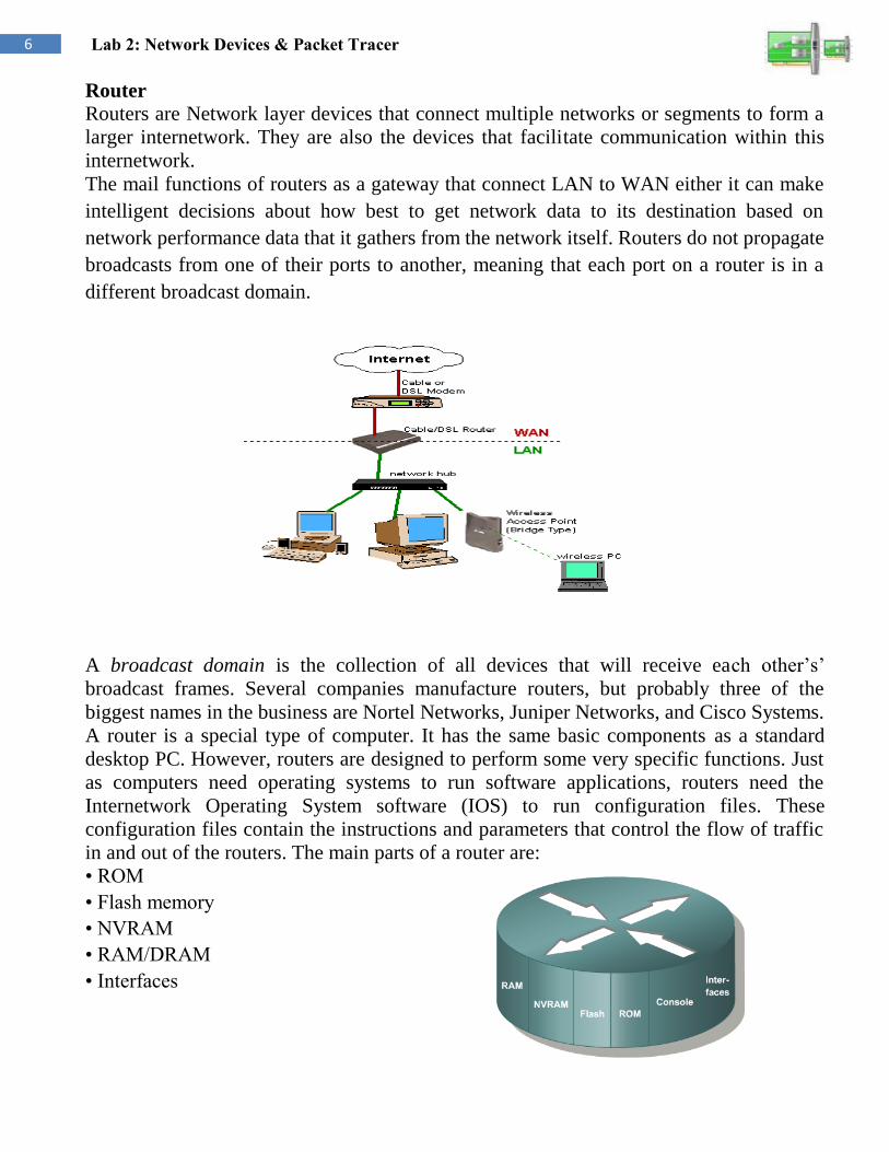
in and out of the routers. The main parts of a router are:
• ROM
• Flash memory
• NVRAM
• RAM/DRAM
• Interfaces
7 Lab 2: Network Devices & Packet Tracer
Read-only memory (ROM) Loads the bootstrap program that initializes the router’s basic hardware components. It’s
not modified during normal operations, but it can be upgraded with special plug-in chips.
The content of ROM is maintained even when the router is rebooted
Flash memory A type of erasable, programmable, read-only memory (EPROM), not typically modified
during normal operations. However, it can be upgraded or erased when necessary the
content of flash memory is maintained even when the router is rebooted.
Flash memory contains the working copy of the current Cisco IOS.Is the component that
initializes the IOS for normal router operations.
Nonvolatile random access memory (NVRAM) A special type of RAM that is not cleared when the router is rebooted .The startup
configuration file for the router is stored in NVRAM by default .This is the first file
created by the person who sets up the router The Cisco IOS uses the configuration file in
NVRAM during the router boot process
Random access memory (RAM) Also known as dynamic random access memory (DRAM) is a volatile hardware
component, its information is not maintained in the event of a router reboot changes to the
router’s running configuration take place in RAM/DRAM.
Router Interfaces:
Management ports Routers have physical connectors that are used to manage the router. These connectors are
known as management ports. Unlike Ethernet and serial interfaces, management ports are
not used for packet forwarding. The most common management port is the console port.
The console port is used to connect a terminal, or most often a PC running terminal
emulator software, to configure the router without the need for network access to that
router. The console port must be used during initial configuration of the router.
Another management port is the auxiliary port. Not all routers have auxiliary ports. At
times the auxiliary port can be used in ways similar to a console port. It can also be used
to attach a modem.
Network Interfaces The term interface refers to a physical connector on the router whose main purpose is to
receive and forward packets. Routers have multiple interfaces that are used to connect to
multiple networks. Typically, the interfaces connect to various types of networks, which
mean that different types of media and connectors are required. Often a router will need to
have different types of interfaces. For example, a router usually has FastEthernet
interfaces for connections to different LANs and various types of WAN interfaces to
connect a variety of serial links including T1, DSL and ISDN.

8 Lab 2: Network Devices & Packet Tracer
Like interfaces on a PC, the ports and interfaces on a router are located on the
outside of the router. Their external location allows for convenient attachment to the
appropriate network cables and connectors.
Like most networking devices, routers use LED indicators to provide status information.
An interface LED indicates the activity of the corresponding interface. If an LED is off
when the interface is active and the interface is correctly connected, this may be an
indication of a problem with that interface. If an interface is extremely busy, its LED will
always be on. Depending on the type of router, there may be other LEDs as well.
Router Switch
Layer: Network Layer (Layer 3
devices)
Data Link Layer (Layer 2
devices)
Transmission Type: At Initial Level Broadcast
then Uni-cast & Multicast
At Initial Level Broadcast
then Uni-cast & Multicast
Table: Store IP address in Routing
table and maintain address at
its own.
Store MAC address in lookup
table and maintain address at
its own, Switch can Learn
MAC address.
Usage: LAN & WAN LAN
Collision: No collisions. In Full Duplex Switch no
Collision occurs.
Ports: 2/4/8 24/48 ports
Transmission Mode: Full duplex Full duplex
Data Transmission form: Packet Frame (L2 Switch) Frame &
Packet (L3 switch)
Speed: 1-10 Mbps(Wireless) 100
Mbps (Wired)
10/100Mbps, 1Gbps
Broadcast Domain: Every port has its own
Broadcast domain.
Switch has one broadcast
domain.
Routing Decision: Take faster Routing Decision Take more time for
complicated routing Decision
9 Lab 2: Network Devices & Packet Tracer
Layer 3 Switches A Network layer device that has received much media attention of late is the Layer 3
Switch.
The Layer 3 part of the name corresponds to the Network layer of the OSI model. It
performs the multiport, virtual LAN, data-pipelining functions of a standard Layer 2
Switch, but it can also perform basic routing functions between virtual LANs.
Gateways A gateway is any hardware and software combination that connects dissimilar network
environments. Gateways are the most complex of network devices because they perform
translations at multiple layers of the OSI model. Router considered as a gateway because
it combine LAN environment and WAN environment.
Other Devices In addition to these network connectivity devices, there are several devices that, while
maybe not directly connected to a network, participate in moving network data:
• Modems
• CSU/DSUs
• Firewalls
Modems A modem is a device that modulates digital data onto an analog carrier for transmission
over an analog medium and then demodulates from the analog carrier to a digital signal
again at the receiving end. The term modem is actually an acronym that stands for
Modulator/Demodulator.
When we hear the term modem, different types should come to mind:
• Traditional (POTS)
• DSL
Traditional (POTS) Most modems you find in computers today fall into the category of traditional modems.
These modems convert the signals from your computer into signals that travel over the
plain old telephone service (POTS) lines. The majority of modems that exist today are
POTS modems, mainly because PC manufacturers include one with a computer.
A router is assigned the gateway address for all the devices on the LAN. One purpose of
a router is to serve as an entry point for packets coming into the network and exit point
for packets leaving the network. Gateway addresses are very important to users. Cisco
estimates that 80 percent of network traffic will be destined to devices on other
networks, and only 20 percent of network traffic will go to local devices. If a gateway
cannot be reached by the LAN devices, users will not be able to perform their job.
10 Lab 2: Network Devices & Packet Tracer
DSL Digital subscriber line (DSL) is quickly replacing traditional modem access because it
offers higher data rates for a reasonable cost. In addition, you can make regular phone
calls while online. DSL uses higher frequencies (above 3200Hz) than regular voice phone
calls use, which provides greater bandwidth (up to several megabits per second) than
regular POTS modems provide while still allowing the standard voice frequency range to
travel at its normal frequency to remain compatible with traditional POTS phones and
devices. DSL “modems” are the devices that allow the network signals to pass over phone
lines at these higher frequencies.
Most often, when you sign up for DSL service, the company you sign up with will send
you a DSL modem for free or for a very low cost. This modem is usually an external
modem, and it usually has both a phone line and an Ethernet connection. You must
connect the phone line to a wall jack and the Ethernet connection to your computer (you
must have an Ethernet NIC in your computer in order to connect to the DSL modem).
Alternatively, a router, hub, or switch may be connected to the Ethernet port of the DSL
modem, increasing the options available for the Ethernet network.
If you have DSL service on the same phone line you use to make voice calls, you must
install DSL filters on all the phone jacks where you have a phone. Or, a DSL filter will be
installed after the DSL modem for all the phones in a building. Otherwise, you will hear a
very annoying hissing noise (the DSL signals) on your voice calls.
CSU/DSUs
The Channel Service Unit/Data Service Unit (CSU/DSU) is a common device found in
equipment rooms when the network is connected via a T-series data connection or other
digital serial technology such as T1 connection. It is essentially two devices in one that are
used to connect a digital carrier to your network equipment. The Channel Service Unit
(CSU) terminates the line at the customer’s premises. It also provides diagnostics and
remote testing, if necessary. The Data Service Unit (DSU) does the actual transmission of
the signal through the CSU. It can also provide buffering and data flow control.
Firewalls A firewall is probably the most important device on a network if that network is connected
to the Internet. Its job is to protect LAN resources from attackers on the Internet.
Similarly, it can prevent computers on the network from accessing various services on the
Internet. It can be used to filter packets based on rules that the network administrator sets.
These rules state what kinds of information can flow into and out of a network’s
connection to the Internet.
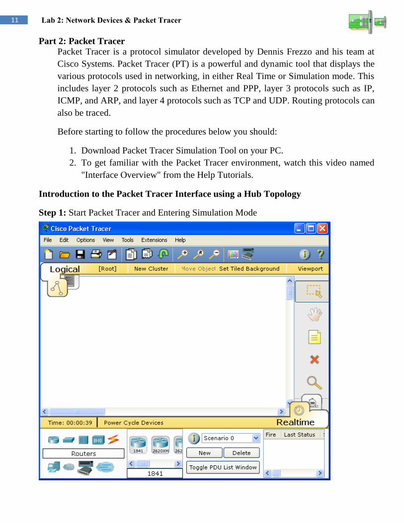
11 Lab 2: Network Devices & Packet Tracer
Part 2: Packet Tracer
Packet Tracer is a protocol simulator developed by Dennis Frezzo and his team at
Cisco Systems. Packet Tracer (PT) is a powerful and dynamic tool that displays the
various protocols used in networking, in either Real Time or Simulation mode. This
includes layer 2 protocols such as Ethernet and PPP, layer 3 protocols such as IP,
ICMP, and ARP, and layer 4 protocols such as TCP and UDP. Routing protocols can
also be traced.
Before starting to follow the procedures below you should:
1. Download Packet Tracer Simulation Tool on your PC.
2. To get familiar with the Packet Tracer environment, watch this video named
"Interface Overview" from the Help Tutorials.
Introduction to the Packet Tracer Interface using a Hub Topology
Step 1: Start Packet Tracer and Entering Simulation Mode

12 Lab 2: Network Devices & Packet Tracer
Step 2: Choosing Devices and Connections
We will begin building our network topology by selecting devices and the media in
which to connect them. Several types of devices and network connections can be
used. For this lab we will keep it simple by using End Devices, Switches, Hubs, and
Connections. Single click on each group of devices and connections to display the
various choices.
Step 3: Building the Topology – Adding Hosts
Single click on the End Devices.
Single click on the Generic host.
Move the cursor into topology area. You will notice it turns into a plus “+”
sign. Single click in the topology area and it copies the device.
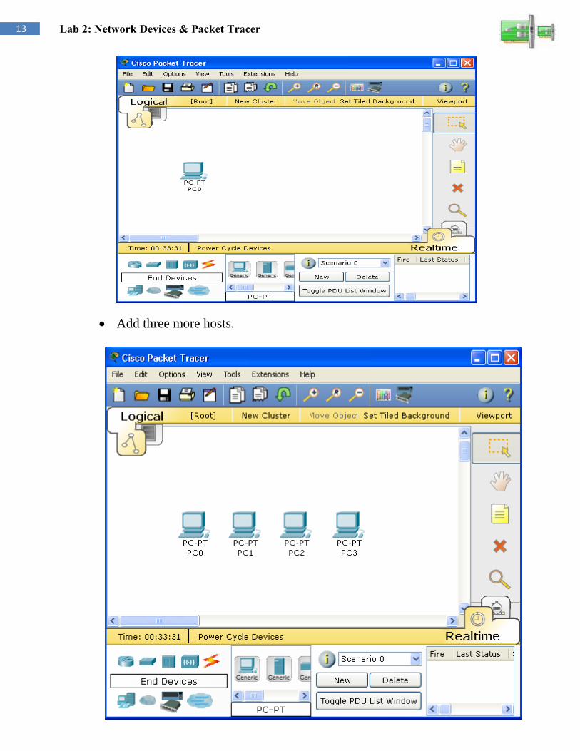
13 Lab 2: Network Devices & Packet Tracer
Add three more hosts.

14 Lab 2: Network Devices & Packet Tracer
Step 4: Building the Topology – Connecting the Hosts to Hubs and Switches
Adding a Hub: Select a hub, by clicking once on Hubs and once on a Generic
hub.
Connect PC0 to Hub0 by first choosing Connections.
Click once on the Copper Straight-through cable.
Perform the following steps to connect PC0 to Hub0:
1. Click once on PC0
2. Choose Fast Ethernet
3. Drag the cursor to Hub0
4. Click once on Hub0 and choose Port0
5. Notice the green link lights on both the PC0 Ethernet NIC and the Hub0 Port0
showing that the link is active.
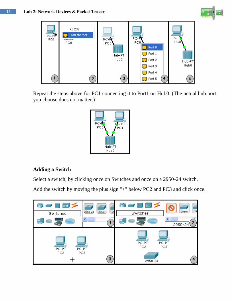
15 Lab 2: Network Devices & Packet Tracer
Repeat the steps above for PC1 connecting it to Port1 on Hub0. (The actual hub port
you choose does not matter.)
Adding a Switch
Select a switch, by clicking once on Switches and once on a 2950-24 switch.
Add the switch by moving the plus sign "+" below PC2 and PC3 and click once.

16 Lab 2: Network Devices & Packet Tracer
Connect PC2 to Switch0 by first choosing Connections.
Click once on the Copper Straight-through cable.
Perform the following steps to connect PC2 to Switch0:
1. Click once on PC2
2. Choose FastEthernet
3. Drag the cursor to Switch0
4. Click once on Switch0 and choose FastEthernet0/1
5. Notice the green link lights on PC2 Ethernet NIC and amber light Switch0
FastEthernet0/1 port. The switch port is temporarily not forwarding frames,
while it goes through the stages for the Spanning Tree Protocol (STP)
process.
6. After a about 30 seconds the amber light will change to green indicating that
the port has entered the forwarding stage. Frames can now be forwarded out
the switch port.
Repeat the steps above for PC3 connecting it to Port3 on switch0 on port
FastEthernet0/2. (The actual switch port you choose does not matter.)

17 Lab 2: Network Devices & Packet Tracer
Move the cursor over the link light to view the port. Fa means
FastEthernet, 100 Mbps Ethernet.
Step 5: Configuring IP Addresses and Subnet Masks on the Hosts
Before we can communicate between the hosts we need to configure IP Addresses
and Subnet Masks on the devices.
Click once on PC0.
Choose the Config tab. It is here that you can change the name of PC0. It is also
here where you would enter a Gateway IP Address, also known as the default
gateway. We will discuss this later, but this would be the IP address of the local
router. If you want, you can enter the IP Address 192.168.1.1.

18 Lab 2: Network Devices & Packet Tracer
Click on FastEthernet. Although we have not yet discussed IP Addresses, add
the IP Address to 192.168.1.10. Click once in the Subnet Mask field to enter the
default Subnet Mask. You can leave this at 255.255.255.0. We will discuss this
later.

19 Lab 2: Network Devices & Packet Tracer
Also, notice this is where you can change the Bandwidth (speed) and
Duplex of the Ethernet NIC (Network Interface Card). The default is Auto
(autonegotiation), which means the NIC will negotiate with the hub or switch. The
bandwidth and/or duplex can be manually set by removing the check from the Auto
box and choosing the specific option.
Bandwidth – Auto
If the host is connected to a hub or switch port which can do 100 Mbps, then the
Ethernet NIC on the host will choose 100 Mbps (Fast Ethernet). Otherwise, if the hub
or switch port can only do 10 Mbps, then the Ethernet NIC on the host will choose 10
Mbps (Ethernet).
Duplex – Auto
Hub: If the host is connected to a hub, then the Ethernet NIC on the host will choose
Half Duplex. Switch: If the host is connected to a switch, and the switch port is
configured as Full Duplex (or Autonegotiation), then the Ethernet NIC on the host
will choose Full Duplex. If the switch port is configured as Half Duplex, then the
Ethernet NIC on the host will choose Half Duplex. (Full Duplex is a much more
efficient option.) The information is automatically saved when entered.
Repeat these steps for the other hosts. Use the information below for IP
Addresses and Subnet Masks.
Verify the information: To verify the information that you entered, move the
Select tool (arrow) over each host.
Host IP Address Subnet Mask
PC0 192.68.1.10 255.255.255.0
PC1 192.68.1.11 255.255.255.0
PC2 192.68.1.12 255.255.255.0
PC3 192.68.1.13 255.255.255.0

20 Lab 2: Network Devices & Packet Tracer
Deleting a Device or Link: To delete a device or link, choose the
Delete tool and click on the item you wish to delete.
Step 6: Connecting Hub0 to Switch0
To connect like-devices, like a Hub and a Switch, we will use a Cross-over
cable. Click once the Cross-over Cable from the Connections options.
Move the Connections cursor over Hub0 and click once.
Select Port2 (actual port does not matter).

21 Lab 2: Network Devices & Packet Tracer
Move the Connections cursor to Switch0.
Click once on Switch0 and choose FastEthernet0/3 (actual port does not
matter).
The link light for switch port FastEthernet0/3 will begin as amber and eventually
change to green as the Spanning Tree Protocol transitions the port to forwarding.
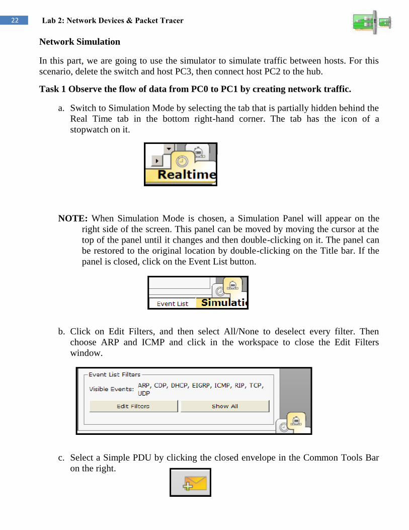
22 Lab 2: Network Devices & Packet Tracer
Network Simulation
In this part, we are going to use the simulator to simulate traffic between hosts. For this
scenario, delete the switch and host PC3, then connect host PC2 to the hub.
Task 1 Observe the flow of data from PC0 to PC1 by creating network traffic.
a. Switch to Simulation Mode by selecting the tab that is partially hidden behind the
Real Time tab in the bottom right-hand corner. The tab has the icon of a
stopwatch on it.
NOTE: When Simulation Mode is chosen, a Simulation Panel will appear on the
right side of the screen. This panel can be moved by moving the cursor at the
top of the panel until it changes and then double-clicking on it. The panel can
be restored to the original location by double-clicking on the Title bar. If the
panel is closed, click on the Event List button.
b. Click on Edit Filters, and then select All/None to deselect every filter. Then
choose ARP and ICMP and click in the workspace to close the Edit Filters
window.
c. Select a Simple PDU by clicking the closed envelope in the Common Tools Bar
on the right.
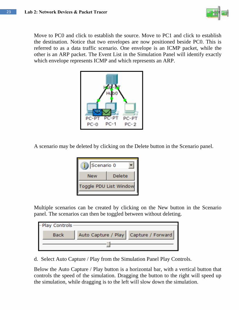
23 Lab 2: Network Devices & Packet Tracer
Move to PC0 and click to establish the source. Move to PC1 and click to establish
the destination. Notice that two envelopes are now positioned beside PC0. This is
referred to as a data traffic scenario. One envelope is an ICMP packet, while the
other is an ARP packet. The Event List in the Simulation Panel will identify exactly
which envelope represents ICMP and which represents an ARP.
A scenario may be deleted by clicking on the Delete button in the Scenario panel.
Multiple scenarios can be created by clicking on the New button in the Scenario
panel. The scenarios can then be toggled between without deleting.
d. Select Auto Capture / Play from the Simulation Panel Play Controls.
Below the Auto Capture / Play button is a horizontal bar, with a vertical button that
controls the speed of the simulation. Dragging the button to the right will speed up
the simulation, while dragging is to the left will slow down the simulation.

24 Lab 2: Network Devices & Packet Tracer
e. Choose the Reset Simulation button in the Simulation window.
Notice that the ARP envelope is no longer present. This has reset the simulation but
has not cleared any configuration changes or MAC / ARP table entries.
f. Choose the Capture / Forward button.
Notice that the ICMP envelope moved forward one device and stopped. The Capture
/ Forward button will allow you to move the simulation one step at a time.
g. Choose the Power Cycle Devices button on the bottom left, above the device
icons.
h. Choose Yes
Notice that both the ICMP and ARP envelopes are now present. The Power Cycle
Devices will clear any configuration changes not saved and clear the MAC / ARP
tables.
Task 2 View ARP Tables on each PC.
a. Choose the Auto Capture / Play button and allow the simulation to run
completely.

25 Lab 2: Network Devices & Packet Tracer
b. Click on PC-0 and select the Desktop tab.
c. Select the Command Prompt and type the command arp -a.
d. Notice that the MAC address for PC2 is in the ARP table (to view the MAC
address of PC2, click on PC2 and select the Config tab).
e. To examine the ARP tables for PC1 and PC2in another way, click on the
Inspect Tool.
Then click on PC1 and the ARP table will appear in a new window.
Note that PC2 does not have an entry in the ARP table yet. Close the ARP Table
window.
f. Click on PC2 to view the ARP table. Then close the ARP Table window.
NOTE: To deactivate the Inspect Tool, click on the Select Tool

26 Lab 2: Network Devices & Packet Tracer
Task 3 Adding routers and installing modules
a. In the Network Component Box, click on the router.
b. Select an 1841 router.
c. Move the cursor to the Logical Workspace and click on the desired location.
NOTE: If multiple instances of the same device are needed press and hold the Ctrl
button, click on the desired device, and then release the Ctrl button. A copy of the device
will be created and can now be move to the desired location.
d. Click on the router to bring up the Configuration Window. This window has
three modes: Physical, Config, and CLI (Physical is the default mode).

27 Lab 2: Network Devices & Packet Tracer
The Physical mode is used to add modules to a device, such as a WAN Interface Card
(WIC). The Config mode is used for basic configuration. Commands are entered in a
simple GUI format, with actual equivalent IOS commands shown in the lower part of the
window. The CLI mode allows for advanced configuration of the device. This mode
requires the user to enter the actual IOS commands just as they would on a live device.
e. In the Physical mode, click on the router power switch to turn the device off.
f. Select the WIC-2T module and drag it to Slot 0 on the router. Then drag a
WIC Cover to Slot1.
g. Power the device back on.
h. Click on the Network Component Box and select Connections. Then select a
Copper Straight-through connection to connect the router to the hub.
NOTE: The Smart Connection can be used to automatically select the appropriate
cable type. However, the user will have no choice as to which interface the connection is
assigned to; it will take the first available appropriate interface.
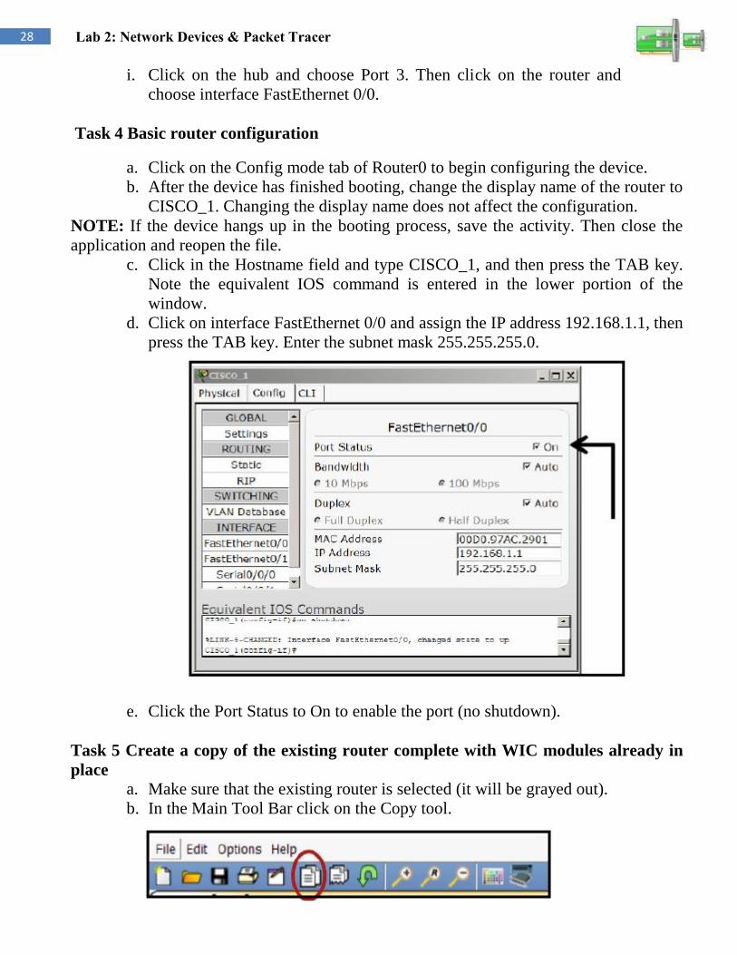
28 Lab 2: Network Devices & Packet Tracer
i. Click on the hub and choose Port 3. Then click on the router and
choose interface FastEthernet 0/0.
Task 4 Basic router configuration
a. Click on the Config mode tab of Router0 to begin configuring the device.
b. After the device has finished booting, change the display name of the router to
CISCO_1. Changing the display name does not affect the configuration.
NOTE: If the device hangs up in the booting process, save the activity. Then close the
application and reopen the file.
c. Click in the Hostname field and type CISCO_1, and then press the TAB key.
Note the equivalent IOS command is entered in the lower portion of the
window.
d. Click on interface FastEthernet 0/0 and assign the IP address 192.168.1.1, then
press the TAB key. Enter the subnet mask 255.255.255.0.
e. Click the Port Status to On to enable the port (no shutdown).
Task 5 Create a copy of the existing router complete with WIC modules already in
place
a. Make sure that the existing router is selected (it will be grayed out).
b. In the Main Tool Bar click on the Copy tool.

29 Lab 2: Network Devices & Packet Tracer
c. Click on the Paste tool and the copied device will appear in the work
area.
d. Drag the new device to the desired location.
e. Click on the Network Component Box and select Connections. Then select the
Serial DCE connection.
f. Click on the CISCO_1 router and connect to the Serial 0/0/0 interface.
g. Click on the new router (copy CISCO_1) and connect to the Serial 0/0/0
interface.
Task 6 Configuring the WAN link
a. Click on the CISCO_1 router and select the Config mode
b. Select interface Serial 0/0/0
c. Configure the interface Serial 0/0/0 with the IP address 192.168.2.1, then press
the TAB key and enter the subnet mask 255.255.255.0 on the interface.
d. Set the clock rate to 56000
e. Click the Port Status to On to enable the port (no shutdown).
f. Click on the new router and select the Config mode.
g. Change the Display Name and Hostname to CISCO_2.
h. Configure the interface Serial 0/0/0 with the IP address 192.168.2.2, then press
the TAB key and enter the subnet mask 255.255.255.0 on the interface.
i. Click the Port Status to On to enable the port (no shutdown).
NOTE: The link lights on the serial link should change from red to green to indicate the
link is active.
Task 7 Configure the routing protocol

30 Lab 2: Network Devices & Packet Tracer
a. Click on the CISCO_1 router and select the Config tab. Then click on
RIP and add the network address 192.168.1.0 and 192.168.2.0.
b. Click on the CISCO_2 router and select the Config tab. Then click on RIP and
add the network address 192.168.2.0.
NOTE: To configure RIP routing protocol, you add the directly connected networks ID IP
addresses to each router.
c. Go to each PC and set the Default Gateway to 192.168.1.1
NOTE: The default gateway is the fastethernet port which the PC is connected to.
Task 8 Set the default gateway on the PCs a. Click on PC0 and select the Config tab. Enter the default gateway address
192.168.1.1.
b. Click on PC1 and select the Config tab. Enter the default gateway address
192.168.1.1.
c. Click on PC2 and select the Config tab. Enter the default gateway address
192.168.1.1.
Task 9 Test the connectivity of the network
a. Click on the Simulation mode.
b. Select a Simple PDU and click on PC-A as the source, then click on
Cisco_2 as the destination. The ping should be successful.
c. Test the ICMP packet sent from PC1 to CISCO_1 (first open the simulation
mode and then open the info box that appears on the event list window to the
right of the ICMP packet sent from PC1 to CISCO_1).
Task 10 Save the Packet Tracer file
a. Save the Packet Tracer file as PT Basic.

University of Jordan
Faculty of Engineering & Technology
Computer Engineering Department
Computer Networks Laboratory
907528
Lab 3: Basic Device Configuration
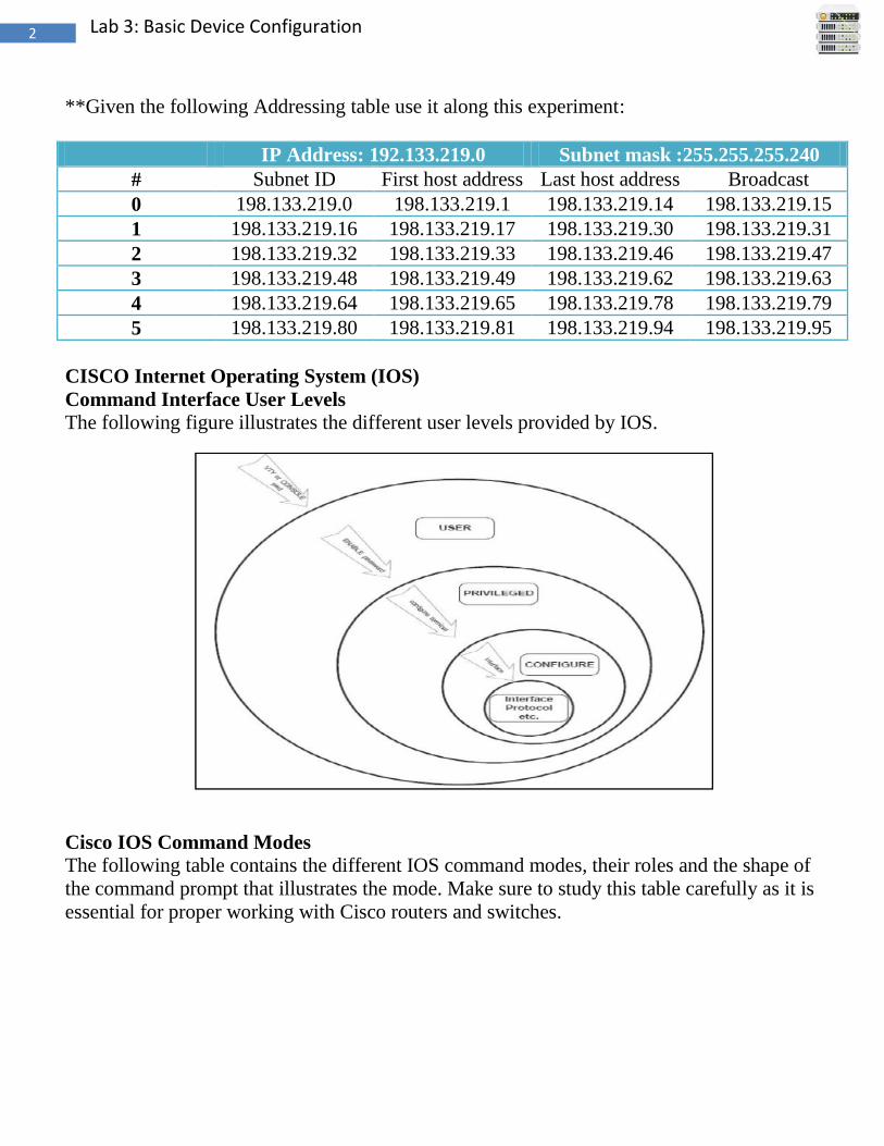
2 Lab 3: Basic Device Configuration
**Given the following Addressing table use it along this experiment:
IP Address: 192.133.219.0 Subnet mask :255.255.255.240
# Subnet ID First host address Last host address Broadcast
0 198.133.219.0 198.133.219.1 198.133.219.14 198.133.219.15
1 198.133.219.16 198.133.219.17 198.133.219.30 198.133.219.31
2 198.133.219.32 198.133.219.33 198.133.219.46 198.133.219.47
3 198.133.219.48 198.133.219.49 198.133.219.62 198.133.219.63
4 198.133.219.64 198.133.219.65 198.133.219.78 198.133.219.79
5 198.133.219.80 198.133.219.81 198.133.219.94 198.133.219.95
CISCO Internet Operating System (IOS)
Command Interface User Levels The following figure illustrates the different user levels provided by IOS.
Cisco IOS Command Modes The following table contains the different IOS command modes, their roles and the shape of
the command prompt that illustrates the mode. Make sure to study this table carefully as it is
essential for proper working with Cisco routers and switches.

3 Lab 3: Basic Device Configuration
User Exec Mode
The user EXEC mode is entered when the router is accessed via a serial connection or when
accessing the router via telnet.
The command prompt of the user EXEC mode is:
Router1>
The user EXEC mode only offers a small set of commands, such as ping, telnet, and traceroute.
Configuration parameters cannot be read or modified in this mode
Logging the user off, type:
Router1> exit
Privileged EXEC Mode
To change or view configuration information of a router, user must enter system
administrator mode called Privileged EXEC Mode
The privileged EXEC mode is used to read configuration files, reboot the router, and set
operating parameters.
Entering the privileged EXEC mode requires to type a password, called the enable
secret.
The privileged EXEC mode is entered by this command:
Router1>enable
If a password is set, then the system will require it at this stage.
Typing the password displays the following command prompt:
Router1#
4 Lab 3: Basic Device Configuration
Global Configuration Mode The global configuration mode is used to modify system wide configuration parameters,
such as routing algorithms and routing tables.
This is done by typing:
Router1#Configure terminal
The argument terminal tells the router that the configuration commands will be entered
from a terminal. The alternatives are to issue configuration commands from a configuration
file or from a remote machine via a file transfer
The command prompt in the global configuration mode is:
Router1(Config)#
Notes:
commands in the current command mode
Router1(config-if)#?
Router1#configure ?
If a certain command enables a feature of a router than adding a “no” in front of that command
disables the same feature. Sometimes it is the other way around, that is, the command to enable
a feature uses the command to disable the feature preceded by a “no”.
Examples:
Enable IP forwarding: ip routing
Disable IP forwarding: no ip routing
Add a routing table entry: ip route 10.0.2.0 255.255.255.0 10.0.3.1
Notes:
commands in the current command mode
Router1(config-if)#?
This command helps to determine if a command can be executed in the current mode
The question mark can also be used to determine the list of available options of a
command.
Router1#configure ?
If a certain command enables a feature of a router than adding a “no” in front of that command
disables the same feature. Sometimes it is the other way around, that is, the command to
enable a feature uses the command to disable the feature preceded by a “no”.
Examples:
Enable IP forwarding: ip routing
Disable IP forwarding: no ip routing
Add a routing table entry: ip route 10.0.2.0 255.255.255.0 10.0.3.1
Delete a routing table entry: no ip route 10.0.2.0 255.255.255.0 10.0.3.1
Disable a network interface: shutdown
Enable a network interface: no shutdown

5 Lab 3: Basic Device Configuration
Delete a routing table entry: no ip route 10.0.2.0 255.255.255.0 10.0.3.1
Disable a network interface: shutdown
Enable a network interface: no shutdown
Establishing a Console Session with HyperTerminal HyperTerminal is a simple Windows-based terminal emulation program for serial
communication that can be used to connect to the console port on Cisco IOS devices. A serial
interface on a computer is connected to the Cisco device via a rollover cable. Using
HyperTerminal is the most basic way to access a router for checking or changing its
configuration.
Steps: 1- Connect the console (rollover) cable to the console port on the router. Connect the other
cable end to the host computer with a DB-9 adapter to the COM 1 port.
2- From the Windows taskbar, start the HyperTerminal program by clicking Start >
Programs >Accessories > Communications > HyperTerminal.
3- At the Connection Description window, enter a session name in the Name field. Select
an appropriate icon, or leave the default. Click OK.
4- Enter the appropriate connection type, COM 1, in the Connect using field. Click OK.
5- The settings in the Hyper Terminal need to be set correctly; otherwise, "strange-looking"
or garbage characters may show up on the screen. When you set up the connection, use
these settings:
Here is a screenshot of how to configure these settings on a Windows-based PC running
Hyper Terminal:
Bits per sec : 9600
Data bits : 8
Parity : none
Stop bits : 1
Flow control : none

6 Lab 3: Basic Device Configuration
Without these settings, the router may display but does not accept any keystrokes. The
router, therefore, appears as if it is hung or has crashed. With the correct settings, you
can use Hyper Terminal to configure and monitor the router.
6- There should be a response from the router. This indicates that connection has been
successfully completed.
7- When finished, close the HyperTerminal session. Click File > Exit. When asked whether
to save the session, click Yes. Enter a name for the session.
1- Note: this process is the same for a Switch.
Basic Cisco Device Configuration
Common configuration tasks include setting the hostname, access passwords, and
(Message of the Day Banner) MOTD banner.
Interface configuration is extremely important. In addition to assigning a Layer 3 IP
address, enter a description that describes the destination connection speeds
troubleshooting time.
Configuration changes are effective immediately.
Configuration changes must be saved in NVRAM to be persistent across reboot.
Configuration changes may also be saved off-line in a text file for auditing or device
replacement. Cisco IOS switch configuration is similar to Cisco IOS router
configuration.
Configure Cisco Router Global Configuration Settings.
1- Physically connect devices.
Connect the console or rollover cable to the console port on the router. Connect the other end
of the cable to the host computer using a DB-9 or DB-25 adapter to the COM 1 port. Connect
the crossover cable between the host computer’s network interface card (NIC) and Router
interface Fa0. Ensure that power has been applied to the host computer and router.
2- Connect host computer to router through HyperTerminal.
Configure HyperTerminal with the proper settings as mentioned in previously in this
experiment. When the HyperTerminal session window comes up, press the Enter key until
there is a response from the router.
If the router terminal is in the configuration mode, exit by typing NO.
Would you like to enter the initial configuration dialog? [yes/no]:no
Press RETURN to get started!

7 Lab 3: Basic Device Configuration
When in privileged exec command mode, any misspelled or unrecognized commands will
attempt to be translated by the router as a domain name. Since there is no domain server
configured, there will be a delay while the request times out. This can take between several
seconds to several minutes. To terminate the wait, simultaneously hold down the
<CTRL><SHIFT>6 keys then release and press x:
Router>enabel
Translating "enabel"...domain server (255.255.255.255) %
Briefly hold down the keys <CTRL><SHIFT>6, release and press x
Name lookup aborted
Router>
From the user exec mode, enter privileged exec mode:
Router> enable
Verify a clean configuration file with the privileged exec command show running-config. If a
configuration file was previously saved, it will have to be removed.
3- Configure global configuration hostname setting. From the global config mode, there are many different configuration modes that may be
entered. Each of these modes allows the configuration of a particular part or function of the
IOS device. The list below shows a few of them:
Interface mode - to configure one of the network interfaces (Fa0, S0/0,..)
Line mode - to configure one of the lines (physical or virtual) (console, AUX, VTY,..)
Router mode - to configure the parameters for one of the routing protocols
From the privileged exec mode, enter global configuration mode:
Router# configure terminal
Router(config)#
Set the device hostname to Router1:
Router(config)# hostname Router1
Router1(config)#
4- Configure the MOTD banner.
In production networks, banner content may have a significant legal impact on the
organization. For example, a friendly “Welcome” message may be interpreted by a court that
an attacker has been granted permission to hack into the router. A banner should include
information about authorization, penalties for unauthorized access, connection logging,
and applicable local laws. The corporate security policy should provide policy on all banner
messages.
Router1(config)# banner motd % Your Message%

8 Lab 3: Basic Device Configuration
Configure Cisco router password access Access passwords are set for the privileged exec mode and user entry point such as console,
aux, and virtual lines. The privileged exec mode password is the most critical password, since
it controls access to the configuration mode.
1- Configure the privileged exec password.
Cisco IOS supports two commands that set access to the privileged exec mode. One command,
enable password, contains weak cryptography and should never be used if the enable secret
command is available. The enable secret command uses a very secure MD5 cryptographic hash
algorithm. Cisco says “As far as anyone at Cisco knows, it is impossible to recover an enable
secret based on the contents of a configuration file (other than by obvious dictionary attacks).”
Password security relies on the password algorithm, and the password. . In production
environments, strong passwords should be used at all times. A strong password consists of at
least nine characters of upper and lower case letters, numbers, and symbols. In a lab
environment, we will use weak passwords. Set the privileged exec password to cisco.
Router1(config)# enable secret cisco
Router1(config)#
2- Configure the console password
Set the console access password to class. The console password controls console access to the
router.
Router1(config)# line console 0
Router1(config-line)# password class
Router1(config-line)# login
3- Configure the virtual line password.
Set the virtual line access password to class. The virtual line password controls Telnet access
to the router. In early Cisco IOS versions, only five virtual lines could be set, 0 through 4. In
newer Cisco IOS versions, the number has been expanded. Unless a telnet password is set,
access on that virtual line is blocked.
Router1(config-line)# line vty 0 4
Router1(config-line)# password class
Router1(config-line)# login
Notes: There are 16 virtual lines that can be configured on a Cisco switch, 0 through 15.
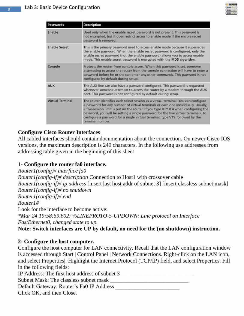
9 Lab 3: Basic Device Configuration
Configure Cisco Router Interfaces All cabled interfaces should contain documentation about the connection. On newer Cisco IOS
versions, the maximum description is 240 characters. In the following use addresses from
addressing table given in the beginning of this sheet
1- Configure the router fa0 interface.
Router1(config)# interface fa0
Router1(config-if)# description Connection to Host1 with crossover cable
Router1(config-if)# ip address [insert last host addr of subnet 3] [insert classless subnet mask]
Router1(config-if)# no shutdown
Router1(config-if)# end
Router1#
Look for the interface to become active:
*Mar 24 19:58:59.602: %LINEPROTO-5-UPDOWN: Line protocol on Interface
FastEthernet0, changed state to up.
Note: Switch interfaces are UP by default, no need for the (no shutdown) instruction.
2- Configure the host computer. Configure the host computer for LAN connectivity. Recall that the LAN configuration window
is accessed through Start | Control Panel | Network Connections. Right-click on the LAN icon,
and select Properties|. Highlight the Internet Protocol (TCP/IP) field, and select Properties. Fill
in the following fields:
IP Address: The first host address of subnet 3__________________________
Subnet Mask: The classless subnet mask ____________________________
Default Gateway: Router’s Fa0 IP Address _______________________
Click OK, and then Close.

10 Lab 3: Basic Device Configuration
Open a terminal window from start| programs|accessories|CommandPrompt, and verify
network settings with the ipconfig command.
3- Verify network connectivity.
Use the ping command to verify network connectivity with the router.
From the router hyperterminal session issue the following command.
Router1# ping <enter the host PC IP address>.
And from the command prompt window on the host computer, issue the following command
C:\Documents and Settings\admin> ping <enter Router’s Fa0 IP Address >
If ping replies are not successful troubleshoot the connection:
tatus using the command
Router1# show ip interface brief
The up in the Status column shows that this interface is operational at Layer 1. The up in
the Protocol column indicates that the Layer 2 protocol is operational. If you find
administratively down in the Status column, then this interface was not enabled with the no
shutdown command.
Verify host computer configuration with the ipconfig command.
Verify the cable connection between the router Fast Ethernet interface and the host
computer Ethernet card is crossover cable.
Note: Turn-off the firewall.
Use TFTP to Save Configuration files and IOS Images Verify network connectivity between your PC and the router using the ping command. The
ping replies must be successful.
Start t the TFTP server. If the computer is properly connected, there is no configuration of the
Cisco TFTP server needed.
Note: Your host computer is considered to be the TFTP server.

11 Lab 3: Basic Device Configuration
From the privileged EXEC prompt, issue the copy running-config tftp command. Follow the
prompts:
Router1#copy running-config tftp:
Address or name of remote host []?<enter TFTP server IP address>
Destination filename [router1-confg]? <ENTER>
!!
667 bytes copied in 0.036 secs (18528 bytes/sec)
Verify a successful upload transfer. Check the TFTP server log file. Click View > Log File.
The output should be similar to the following:
Mon Sep 16 14:10:08 2003: Receiving ‘running-config’ file from
192.168.14.1 in binary mode
Mon Sep 16 14:11:14 2003: Successful.
Note: You can save a back up of the startup-config file in the same way.
Similar to uploading a configuration file, the IOS can also be stored off-line for future use. To
discover the IOS filename, issue the Cisco IOS command show version. The filename is
highlighted, below:
Router1# show version
Cisco IOS Software, 1841 Software (C1841-ADVIPSERVICESK9-M), Version 12.4(10b),
RELEASE SOFTWARE (fc3)
Technical Support: http://www.cisco.com/techsupport
Copyright (c) 1986-2007 by Cisco Systems, Inc.
Compiled Fri 19-Jan-07 15:15 by prod_rel_team
ROM: System Bootstrap, Version 12.4(13r)T, RELEASE SOFTWARE (fc1)
Router1 uptime is 17 minutes
System returned to ROM by reload at 16:47:54 UTC Sun Mar 25 2007
System image file is "flash:c1841-advipservicesk9-mz.124-10b.bin"
*********************************************************
Or enter show flash command to view the IOS filename. Highlight the filename and copy it,
later when you are prompted to enter the flash file name use the mouse right click and select
paste to host.
The commands to upload the IOS are similar to uploading the configuration file:
Router1# copy flash tftp
Source filename []? c1841-advipservicesk9-mz.124-10b.bin
Address or name of remote host []? <enter TFTP server IP address>
Destination filename [c1841-advipservicesk9-mz.124-10b.bin]?
!!!!!!!!!!!!!!!!!!!!!!!!!!!!!!!!!!!!!!!!!!!!!!!!!!!!!!!!!!!!!!!!!!!!!!!!!!!!!!!!!!!!!!!!
22063220 bytes copied in 59.564 secs (370412 bytes/sec)
Router1#

12 Lab 3: Basic Device Configuration
Use TFTP to Restore Configuration files and IOS Images Assume that the configuration on the router has become corrupt and copy the backup startup-
config file from the tftp server to the running-config of the router. To simulate this, change the
hostname of the router from "Router1" to "Router".
Issue the following commands to copy the startup-config file from the TFTP server to the
router.
Router#copy tftp running-config
Address or name of remote host []?<enter TFTP server IP address>
Source filename []? startup-config
Destination filename [running-config]? [Enter]
Accessing tftp://192.168.14.2/startup-config...
Loading startup-config from 192.168.14.2 (via FastEthernet0): !
[OK - 667 bytes]
667 bytes copied in 9.584 secs (70 bytes/sec)
To copy the IOS image to the TFTP server, from the console session in the privileged EXEC
mode, enter the copy flash tftp command. At the prompt enter the IP address of the TFTP
server. Filenames will vary based on IOS and platform. The filename for your system was
reported in the previous step.
Router1#copy flash tftp
Source filename []?c1841-advipservicesk9-mz.124-10b.bin
Address or name of remote host []?<enter TFTP server IP address>
Destination filename [c1841-advipservicesk9-mz.124-10b.bin]? y
After entering this command and answering the process requests, the student should see the
following output on the console. The process may take a few minutes depending on the size of
the image. Do not interrupt this process.
!!!!!!!!!!!!!!!!!!!!!!!!!!!!!!!!!!!!!!!!!!!!!!!!!!!!!!!!!!!!!!!!!!!!!!!!!!!!!!!!
!!!!!!!!!!!!!!!!!!!!!!!!!!!!!!!!!!!!!!!!!!!!!!!!!!!!!!!!!!!!!!!!!!!!!!!!!!!!!!!!
!!!!!!!!!!!!!!!!!!!!!!!!!!!!!!!!!!!!!!!!!!!
22063220 bytes copied in 59.564 secs (370412 bytes/sec)
Save the Router Configuration File. Cisco IOS refers to RAM configuration storage as running-configuration, and NVRAM
configuration storage as startup-configuration. For configurations to survive rebooting or
power restarts, the RAM configuration must be copied into non-volatile RAM (NVRAM). This
does not occur automatically, NVRAM must be manually updated after any changes are made.
1- Compare router RAM and NVRAM configurations.
Use the Cisco IOS show command to view RAM and NVRAM configurations. The
configuration is displayed one screen at a time. A line containing “-- more -- “indicates that
there is additional information to display. The following list describes acceptable key
responses:

13 Lab 3: Basic Device Configuration
Display the contents of NVRAM. If the output of NVRAM is missing, it is because there is no
saved configuration:
Router1# show startup-config
startup-config is not present
Display the contents of RAM.
Router1#show running-config
2- To erase the NVRAM configuration file: Router1# erase startup-config
Erasing the nvram filesystem will remove all configuration files! Continue? [confirm]
<ENTER>
[OK]
Erase of nvram: complete
Reload the router:
Router1# reload
Proceed with reload? [confirm] <ENTER>
Key Description
<SPACE> Display the next page.
<RETURN> Display the next line.
Q Quit
<CTRL> c Quit
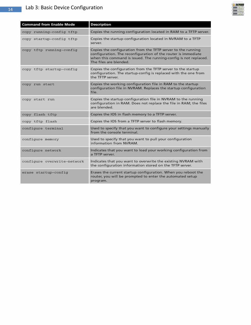
14 Lab 3: Basic Device Configuration

University of Jordan
Faculty of Engineering & Technology
Computer Engineering Department
Computer Networks Laboratory
907528
Lab 4: Basic Network Operation & Troubleshooting

2 Lab 4: Basic Network Operation and Troubleshooting
Part 1: Examining Network Properties Settings
Ipconfig:
The Ipconfig command gets its name from the acronym IP (Internet Protocol) and a
shortened term for configure. It is used to displays all current TCP/IP network configuration
values and refreshes Dynamic Host Configuration Protocol (DHCP) and Domain Name
System (DNS) settings.
Used without parameters, ipconfig displays the IP address, subnet mask, and default gateway
for all adapters.
To get to ipconfig, we have to get to the command line.
Click Start, click Run, type in “cmd” & hit enter.
Type in ipconfig & hit enter. (you can use ipconfig /all for detailed information)You will
get a screen that looks like this.
To find your computers‟ IP number, look next to “IP Address”. To find your router‟s IP
number, look next to “Default Gateway” (listed last). The router here acts as a gateway to the
Internet or another network.

3 Lab 4: Basic Network Operation and Troubleshooting
There are several options available with the ipconfig command, accessible with the command
ipconfig/? To show the most information about the network connections, use the command
ipconfig/all.
This is what the important parts of all that means::
Host name:
This is the host name. This name is configurable, and is selected typically when the machine
is first setup for use. This name can be used by other machines on the network to access this
host.
Connection-specific DNS Suffix:
This will typically give you a clue into what type of connection you have, but it is rarely
needed for troubleshooting.
Description:
This is a description of the Network Adapter.
Physical Address:
This is the MAC Address of the above mentioned Network Adapter. This is a unique
identifier for the hardware. The DHCP server will assign your IP information based on it.
DHCP Enabled:
This is pretty straight-forward. Is DHCP enabled or not? If it is enabled, your IP isDynamic.
If it is not, it is Static.
IP Address:
This is your computer‟s IP address. Note this can differ from the address you are assigned by
your ISP.
4 Lab 4: Basic Network Operation and Troubleshooting
Subnet Mask:
The subnet mask is a pretty complicated thing to explain briefly. The bottom line is if you
want two machines on a LAN to communicate to eachother without the use of a router, the
subnet mask typically needs to match. There are exceptions to this rule.
Default Gateway:
The default gateway is the IP address of the device that will allow communication with the
Internet. In a typical home connection, this is the IP address of your router.
DHCP Server:
This is the IP address of the device responsible for assigning you an IP address, unless you
are using a Static IP. In a typical home connection, this is the IP address of your router.
DNS Servers:
This is the IP address of the device responsible for translating domain names into IP
addresses. I get into more detail about this in my here.
Lease Obtained:
IP addresses assigned by a DHCP server have a lease time. This can be anywhere from a
minute to weeks, months, or even years. This completely depends on the configuration of the
DHCP server. The “Lease Obtained” section shows the date of when the DHCP lease was
obtained.
Lease Expires:
IP addresses assigned by a DHCP server have a lease time. This can be anywhere from a
minute to weeks, months, or even years. This completely depends on the configuration of the
DHCP server. The “Lease Expires” section shows the date of when the DHCP lease is set to
expire. After this date, the IP address assigned to you by the DHCP server may change.
Ipconfig Command Line Options Ipconfig has several command line options that you can utilize. You can display all of them
with the command ipconfig /?. Here is a short selection of the most common uses.
ipconfig /release – Releases all IPv4 addresses (requires DHCP)
ipconfig /renew – Renews all IPv4 addresses (requires DHCP)
ipconfig /flushdns – Flushes the DNS cache
Part 2: Examining Routes
Netstat
On host computers, netstat command displays active TCP connections, ports on which the
computer is listening, Ethernet statistics, the IP routing table, IPv4 statistics, and IPv6
statistics. Used without parameters, netstat displays active TCP connections. There are
several options available with the netstat command, accessible with the command
netstat/?.To display the contents of the IP routing table, use the command netstat –r.
5 Lab 4: Basic Network Operation and Troubleshooting
Route command displays and modifies the entries in the local IP routing table. Used without
parameters, route displays help.
An abbreviated option list for the route command is shown in the table below.
route PRINT Prints active routes
route ADD Adds a route:
route ADD network mask gateway
route DELETE Deletes a route:
route DELETE network
route CHANGE Modifies an existing route
On Cisco routers, show ip route is a common IOS command used to view the routing table of
a router. The route information displayed is much more detailed than the route information
on a host computer.
Part 3: Testing TCP/IP Network Connectivity
Two tools that are indispensable when testing TCP/IP network connectivity are ping and
tracert.
ICMP
ICMP was developed to be a companion to the original Internet Protocol, version 4. With the
creation of IP version 6 (IPv6), a new version of ICMP called ICMP version 6 (ICMPv6) was
created as well, and the original ICMP is now sometimes called ICMPv4 to differentiate it,
just as the “old” IP is now often called “IPv4”. These two versions have some differences in
their specifics, but really are very similar in overall operation.
End host and routers use ICMP as a control, messaging, and diagnostic tool. ICMP utilizes IP
to deliver its messages and is considered an integral part of IP. ICMP messages notify a host
of problems. Although ICMP does not offer a solution to these problems, it can provide
enough information for a source host to solve some of the problems that might occur in the
internetwork. The most popular ICMP message is the echo request and reply. Utilizing the
Ping utility, these messages allow you to test connectivity between end hosts.
Originally created to allow the reporting of a small set of error conditions, ICMP messages
are now used to implement a wide range of error-reporting, feedback and testing capabilities.
While each message type is unique, they are all implemented using a common message
format, sent and received based on relatively simple protocol rules. This makes ICMP one of
the easiest TCP/IP protocols to understand.
ICMP Standards for IPv4 and IPv6
If the host at the specified address receives the Echo request, it responds with an ICMP Echo
Reply datagram. For each packet sent, ping measures the time required for the reply.
As each response is received, ping provides a display of the time between the ping being sent
and the response received. This is a measure of the network performance. Ping has a timeout

6 Lab 4: Basic Network Operation and Troubleshooting
value for the response. If a response is not received within that timeout, ping gives up and
provides a message indicating that a response was not received.
Ping
Ping is a utility for testing IP connectivity between hosts. Ping sends out requests for
responses from a specified host address. Ping uses a Layer 3 protocol that is a part on the
TCP/IP suite called Internet Control Message Protocol (ICMP). Ping uses an ICMP Echo
Request datagram,used for two primary purposes:
To find out if you can reach a host
To find out if a host is responding
Here is the syntax: ping hostname or IP address
Ping sends very small packets to an IP host who will answer by sending packets back.
The ICMP packets sent to the host are called echo_request and the packets sent back
echo_response.If you receive a reply from the destination station, you knowthat you can
reach the host and that it is responding to basic IP requests.

7 Lab 4: Basic Network Operation and Troubleshooting
The Ping results have four ICMP packets have been sent and four received. This result
indicates you that the host is alive at the ICMP level.
In the first case, an external firewall blocks the ICMP requests. ICMP can be used as a first
step in an attack because it can determine the alive hosts before attacking. In this case the
network behind the firewall is hidden from the external world even it is well alive.
Blocking ICMP messages is a first security recommendation to secure a network. The
external firewall is more often used to secure professional network because it is expensive
and requires advanced skills for configuring.
In the second case, the workstation has a personal firewall that blocks the ICMP message. A
personal firewall is recommended for home computers.
In the third case, the "pinged" machine is not connected to the IP network, for instance,
because the network cable is unplugged.Theecho_request message will be discarded on the
last router of the layer 3 device before the remote host.
In the fourth case, the host is down or has its network card deactivated. Such as in the
previous case, the echo_request message will die on the last router of the layer 3 device
before the remote host.

8 Lab 4: Basic Network Operation and Troubleshooting
Step 1 Access the command prompt
Use the Start menu to open the Command Prompt window. Press
Start > Programs > Accessories > Command Prompt or Start > run >cmd
Step 2 Ping the IP address of another computer
In the window, type ping, a space, and the IP address of a computer recorded in the previous
lab.The following figure shows the successful results of ping to this IP address.
Ping uses the ICMP echo request and echo reply feature to test physical connectivity. Since
ping reports on four attempts, it gives an indication of the reliability of the connection. Look
over the results and verify that the ping was successful. Is the ping successful? If not,
perform appropriate troubleshooting.
On a Cisco device, a ping from the IOS will yield to one of several indications for each
ICMP echo that was sent. The most common indicators are:
! : indicates receipt of an ICMP echo reply
. : indicates a timed out while waiting for a reply
U : an ICMP unreachable message was received
Step 3 pings the IP address of the default gateway
Try to ping the IP address of the default gateway. If the ping is successful, it means
there is physical connectivity to the router on the local network and probably the rest of
the world.

9 Lab 4: Basic Network Operation and Troubleshooting
Step 4 Ping the IP address of a DHCP or DNS server
Try to ping the IP address of any DHCP and/or DNS server.
Step 5 Ping the Loopback IP address of this computer
There are some special testing and verification cases for which we can use ping. One case is
for testing the internal configuration of IP on the local host. To perform this test, we ping the
special reserve address of local loopback (127.0.0.1).
A response from 127.0.0.1 indicates that IP is properly installed on the host. This response
comes from the Network layer. This response is not, however, an indication that the
addresses, masks, or gateways are properly configured. Nor does it indicate anything about
the status of the lower layer of the network stack. This simply tests IP down through the
Network layer of the IP protocol. If we get an error message, it is an indication that TCP/IP is
not operational on the host.
Step 6 Ping the hostname of another computer
Try to ping the hostname of the computer of your partner. The figure shows the
successful result of the ping the hostname.

10 Lab 4: Basic Network Operation and Troubleshooting
Look over the results. Notice that the first line of output shows the host name followed by the
IP address. This means the computer was able to resolve the host name to an IP address.
Without name resolution, the ping would have failed because TCP/IP only understands valid
IP addresses, not names.
If the ping was successful, it means that connectivity and discovery of IP addresses can be
done with only a hostname. If successful, then ping a hostname also shows that there is
probably a WINS server working on the network. WINS servers or a local “lmhosts” file
resolve computer host names to IP addresses. If the ping fails, then chances are there is no
NetBIOS name to IP addresses resolution running.
Step 7 ping the Cisco web site
Type the following command: ping www.cisco.com
Step 8 ping the Microsoft web site
Type the following command: ping www.microsoft.com
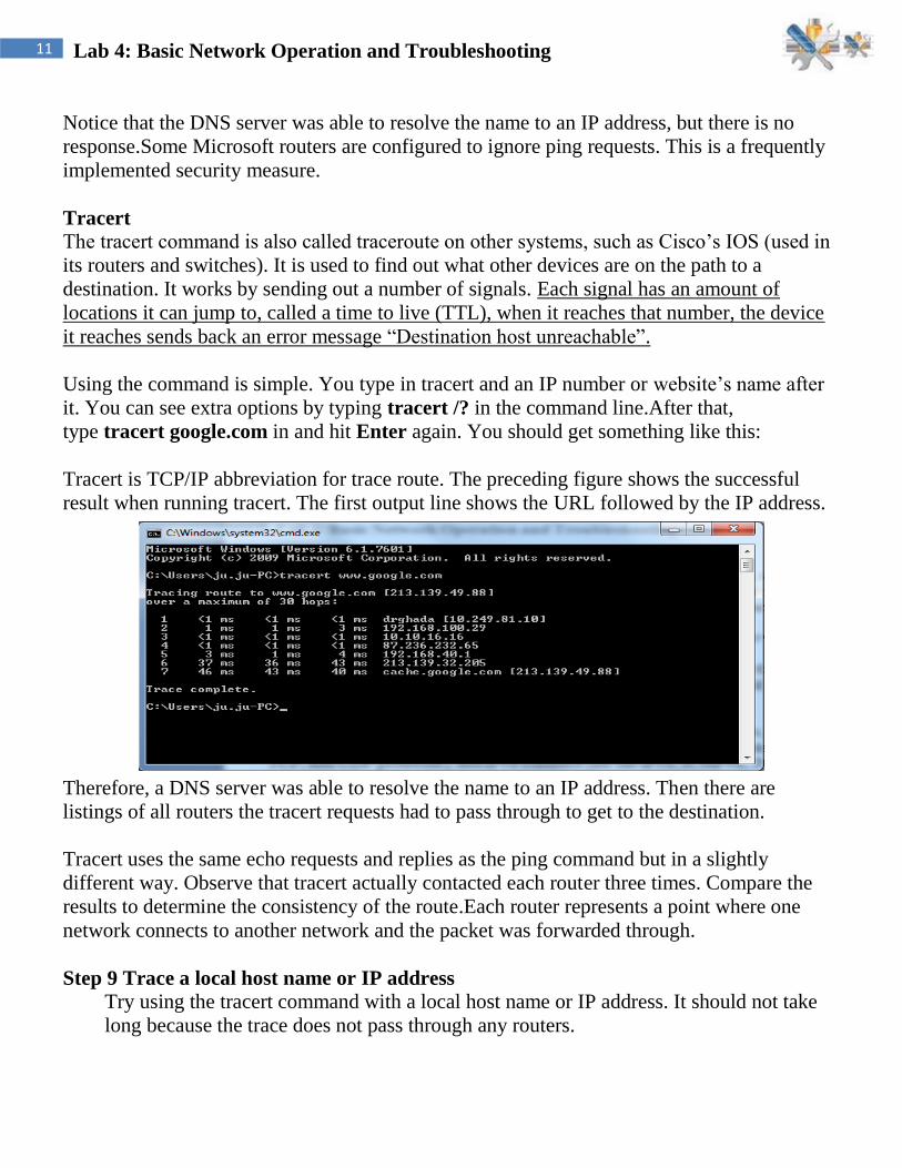
11 Lab 4: Basic Network Operation and Troubleshooting
Notice that the DNS server was able to resolve the name to an IP address, but there is no
response.Some Microsoft routers are configured to ignore ping requests. This is a frequently
implemented security measure.
Tracert
The tracert command is also called traceroute on other systems, such as Cisco‟s IOS (used in
its routers and switches). It is used to find out what other devices are on the path to a
destination. It works by sending out a number of signals. Each signal has an amount of
locations it can jump to, called a time to live (TTL), when it reaches that number, the device
it reaches sends back an error message “Destination host unreachable”.
Using the command is simple. You type in tracert and an IP number or website‟s name after
it. You can see extra options by typing tracert /? in the command line.After that,
type tracert google.com in and hit Enter again. You should get something like this:
Tracert is TCP/IP abbreviation for trace route. The preceding figure shows the successful
result when running tracert. The first output line shows the URL followed by the IP address.
Therefore, a DNS server was able to resolve the name to an IP address. Then there are
listings of all routers the tracert requests had to pass through to get to the destination.
Tracert uses the same echo requests and replies as the ping command but in a slightly
different way. Observe that tracert actually contacted each router three times. Compare the
results to determine the consistency of the route.Each router represents a point where one
network connects to another network and the packet was forwarded through.
Step 9 Trace a local host name or IP address
Try using the tracert command with a local host name or IP address. It should not take
long because the trace does not pass through any routers.
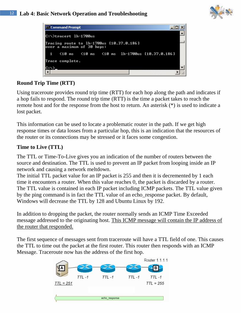
12 Lab 4: Basic Network Operation and Troubleshooting
Round Trip Time (RTT)
Using traceroute provides round trip time (RTT) for each hop along the path and indicates if
a hop fails to respond. The round trip time (RTT) is the time a packet takes to reach the
remote host and for the response from the host to return. An asterisk (*) is used to indicate a
lost packet.
This information can be used to locate a problematic router in the path. If we get high
response times or data losses from a particular hop, this is an indication that the resources of
the router or its connections may be stressed or it faces some congestion.
Time to Live (TTL)
The TTL or Time-To-Live gives you an indication of the number of routers between the
source and destination. The TTL is used to prevent an IP packet from looping inside an IP
network and causing a network meltdown.
The initial TTL packet value for an IP packet is 255 and then it is decremented by 1 each
time it encounters a router. When this value reaches 0, the packet is discarded by a router.
The TTL value is contained in each IP packet including ICMP packets. The TTL value given
by the ping command is in fact the TTL value of an echo_response packet. By default,
Windows will decrease the TTL by 128 and Ubuntu Linux by 192.
In addition to dropping the packet, the router normally sends an ICMP Time Exceeded
message addressed to the originating host. This ICMP message will contain the IP address of
the router that responded.
The first sequence of messages sent from traceroute will have a TTL field of one. This causes
the TTL to time out the packet at the first router. This router then responds with an ICMP
Message. Traceroute now has the address of the first hop.
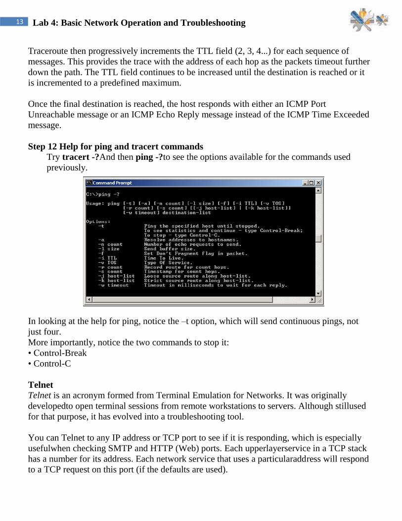
13 Lab 4: Basic Network Operation and Troubleshooting
Traceroute then progressively increments the TTL field (2, 3, 4...) for each sequence of
messages. This provides the trace with the address of each hop as the packets timeout further
down the path. The TTL field continues to be increased until the destination is reached or it
is incremented to a predefined maximum.
Once the final destination is reached, the host responds with either an ICMP Port
Unreachable message or an ICMP Echo Reply message instead of the ICMP Time Exceeded
message.
Step 12 Help for ping and tracert commands
Try tracert -?And then ping -?to see the options available for the commands used
previously.
In looking at the help for ping, notice the –t option, which will send continuous pings, not
just four.
More importantly, notice the two commands to stop it:
• Control-Break
• Control-C
Telnet
Telnet is an acronym formed from Terminal Emulation for Networks. It was originally
developedto open terminal sessions from remote workstations to servers. Although stillused
for that purpose, it has evolved into a troubleshooting tool.
You can Telnet to any IP address or TCP port to see if it is responding, which is especially
usefulwhen checking SMTP and HTTP (Web) ports. Each upperlayerservice in a TCP stack
has a number for its address. Each network service that uses a particularaddress will respond
to a TCP request on this port (if the defaults are used).

14 Lab 4: Basic Network Operation and Troubleshooting
Nslookup
The nslookuputility allows you to query a name server and quickly find out which
nameresolves to which IP address.
Whenever you are configuring a server or workstation to connect to the Internet, you
willalways have to configure DNS if you want name resolution to happen. When configuring
DNS, it is very advantageousto be able to test what IP address DNS is returning to ensure
that it is working properly.
Part 4: Address Resolution Protocol (ARP)
ARP is used as a tool for confirming that a computer is successfully resolving network Layer
3 addresses to Media Access Control (MAC) Layer 2 addresses. While the IP address is
essential to move data from one LAN to another, it cannot deliver the data in the destination
LAN by itself. Local network protocols, like Ethernet use the MAC, or Layer 2, address to
identify local devices and deliver all data.
This is an example of a MAC address:
• 00-02-A5-9A-63-5C
ARP maintains a table in the computer of IP and MAC address combinations. In other words,
it keeps track of which MAC address is associated with an IP address. If ARP does not know
the MAC address of a local device, it issues a broadcast using the IP address. This broadcast
searches for the MAC address that corresponds to the IP address. If the IP address is active
on the LAN, it will send a reply from which ARP will extract the MAC address. ARP will
then add the address combination to the local ARP table of the requesting computer.
When a computer prepares a packet for transmission, it checks the destination IP address to
see if it is part of the local network. It does this by checking to see if the network portion of
the IP address is the same as the local network. If it is, the ARP process is consulted to get
the MAC address of the destination device using the IP address. The MAC address is then
applied to the data packet and used for delivery.
If the destination IP address is not local, the computer will need the MAC address of the
default gateway. The default gateway is the router interface that the local network is
connected to in order to provide connectivity with other networks. The gateway MAC
address is used because the packet will be delivered there and the router will then forward it
to the network it is intended for.
If the computer does not receive any packets from an IP address after a few minutes, it will
drop the MAC/IP entry from the ARP table assuming the device has logged off. Later
attempts to access that IP address will cause ARP to do another broadcast and update the
table.
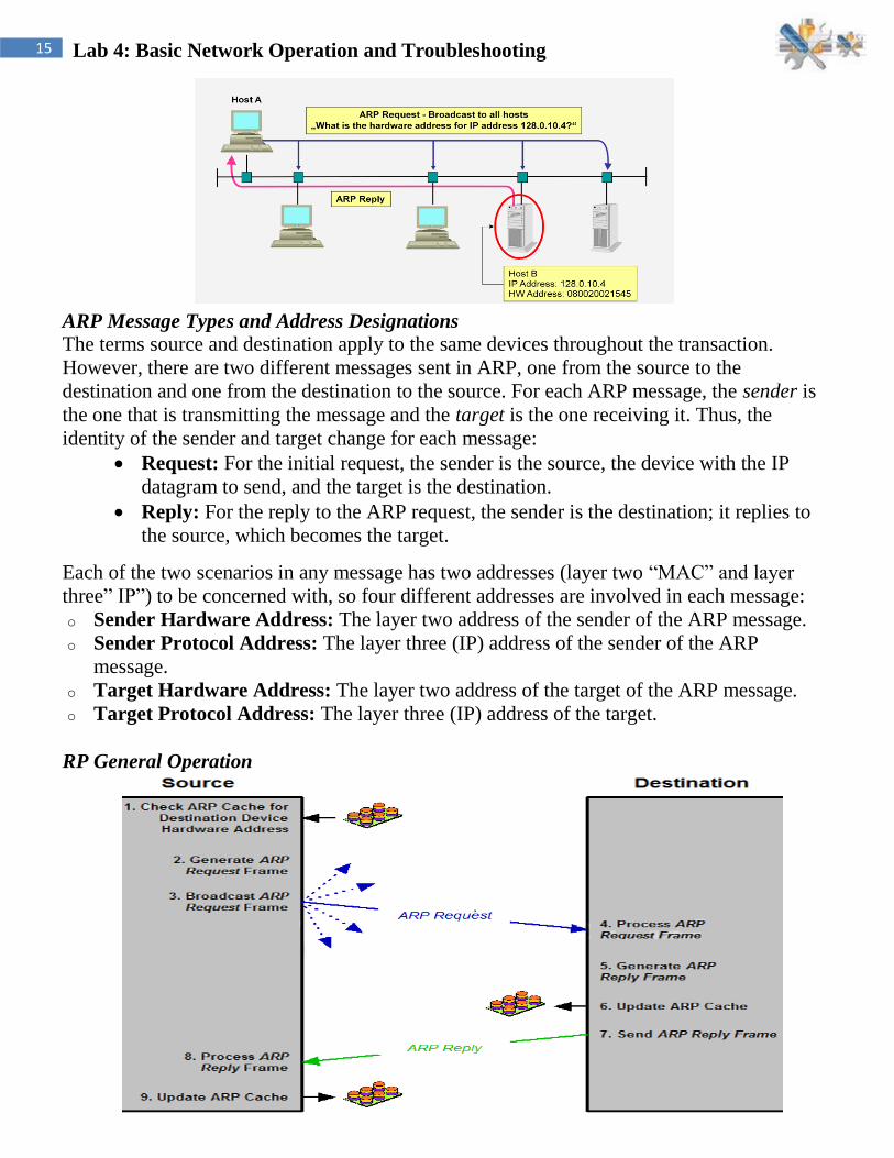
15 Lab 4: Basic Network Operation and Troubleshooting
ARP Message Types and Address Designations The terms source and destination apply to the same devices throughout the transaction.
However, there are two different messages sent in ARP, one from the source to the
destination and one from the destination to the source. For each ARP message, the sender is
the one that is transmitting the message and the target is the one receiving it. Thus, the
identity of the sender and target change for each message:
Request: For the initial request, the sender is the source, the device with the IP
datagram to send, and the target is the destination.
Reply: For the reply to the ARP request, the sender is the destination; it replies to
the source, which becomes the target.
Each of the two scenarios in any message has two addresses (layer two “MAC” and layer
three” IP”) to be concerned with, so four different addresses are involved in each message:
o Sender Hardware Address: The layer two address of the sender of the ARP message.
o Sender Protocol Address: The layer three (IP) address of the sender of the ARP
message.
o Target Hardware Address: The layer two address of the target of the ARP message.
o Target Protocol Address: The layer three (IP) address of the target.
RP General Operation

16 Lab 4: Basic Network Operation and Troubleshooting
To start theArputility in Windows 2000, follow these steps:
1. Choose Start _Run and enter cmd to open the MS-DOS Prompt window. Or, you
canchoose Start _Programs _Accessories _Command Prompt.
2. At the command prompt, typeArpand any switches you need, as discussed later in this
section.
Entered alone, theArpcommand lists only the switches you must use in order to use the arp
utility correctly.
TheArputility is primarily useful for resolving duplicate IP addresses. For example,
yourworkstation receives its IP address from a Dynamic Host Configuration Protocol
(DHCP) server, but it accidentally receives the same address as another workstation. When
you try to ping it, you get no response. Your workstation is trying to determine the MAC
address, and it can‟t do so because two machines are reporting that they have the same IP
address. To solve thisproblem, you can use the arp utility to view your local ARP table and
see which TCP/IP addressis resolved to which MAC address
Step 1 Access a command prompt
Use the Start menu to open the Command Prompt window.
Start > Programs > Accessories > Command Prompt or Start > run >cmd
Step 2 Display the ARP table
1. In the window type arp -a and press Enter. Do not be surprised if there are no entries.
The message displayed will probably be, „No ARP Entries Found‟. Windows
computers remove any addresses that are unused after a couple minutes.
2. Try pinging a couple local addresses and a website URL. Then re-run the command.
The figure below shows a possible result of the arp -a command. The MAC address for
the website will be listed because it is not local, but that will cause the default gateway
to be listed. In the example below 10.36.13.1 is the default gateway while the
10.36.13.92 and 10.36.13.101 are other network computers. Notice that for each IP
address there is a physical address, or MAC, and type, indicating how the address was
learned.
3. From the figure below, it might be logically concluded that the network is 10.36.13.0
and the host computers are represented by 223, 1, 92, and 101.

17 Lab 4: Basic Network Operation and Troubleshooting
Step 3 Use the ARP help feature
Try the command arp -? to see the help feature and look over the options
arp –s[IP Address] [MAC Address]
Simply replace the [IP Address] and [MAC Address] sections with the appropriate entries,
like so: arp –s 204.153.163.5 00–a0–c0–ab–c3–11
You can now take a look at your new ARP table by using the arp –a command. You
shouldsee something like this:
Interface: 204.153.163.3 on Interface 2
Internet Address Physical Address Type
204.153.163.2 00–a0–c9–d4–bc–dc dynamic
204.153.163.4 00–a0–c0–aa–b1–45 dynamic
204.153.163.5 00–a0–c0–ab–c3–11 static
Finally, if you want to delete entries from the ARP table, you can either wait until
thedynamic entries time out, or you can use the –d switch with the IP address of the static
entryyou‟d like to delete, like so:
arp –d 204.153.163.5
This deletes the entry from the ARP table in memory.
The arp utility doesn‟t confirm successful additions or deletions (use arp -a orarp -g for that),
but it will give you an error message if you use incorrect syntax.

18 Lab 4: Basic Network Operation and Troubleshooting
Network Troubleshooting Basics: Some Simple Steps
All tools covered in the previous parts (ping,Ipconfig, tracert) will be combined into a
troubleshooting method. This guide will teach you valuable steps in finding where a problem
is on a network connection.
A working connection shows you what is supposed to happen. If you see something
different, you will know something is up. When problems strike, at the least you can get an
idea of what is going on.
Step 0: Check the Cords & Power
The first thing you should always do is check to make sure everything is plugged in: your
computer, router, device, etc. Many laptops have a button to turn off the wireless connection;
the icon looks like a signal tower.
Step 1: Ping Yourself
You want to test that your machine is working properly. To do this, you want to ping
yourself. You use the loop-back address (127.0.0.1) to do this. Pinging the loop-back address
tests to make sure software on your computer is working properly. Typically, if something is
not working at this stage, you may just need to restart your computer.
Step 2: Ping Your Router
The next step would be to ping your router. You can find your router‟s IP address with
Ipconfig as well. Remember that Ipconfig lists your router as the “Default Gateway.”
This is done to test if your router is responding. If it is not, and you have already checked to
make sure it is on, then it may need to be turned off and turned on. Every once in a while it
may need a refresh. If the problem continues, contact you ISP for assistance to see if they can
help.
Step 3: Ping Yourself with Your IP Address
We want to test to make sure everything is working correctly between your router and your
computer. To do this, ping your IP address. It is listed in the Ipconfig command at the same
time the router IP number is. If this works, you can be pretty confident that a problem is
outside your home network.
Step 4: Ping and Tracert outside Your Network
From here, you want to test something outside your network. In a medium or larger network
setting, a server on another branch of the network will do. For a home network, the Internet
is often your only option. Since chances are the problem is that one or more websites are (or
seem) down, this is a logical thing to check.

University of Jordan
Faculty of Engineering & Technology
Computer Engineering Department
Computer Networks Laboratory
907528
IPv4 Address Subnetting

2 IPv4 Address Subnetting
Internet Protocol Version 4 (IPv4):
Even though the name seems to imply that it's the fourth iteration of the key Internet
Protocol, version 4 of IP was the first that was widely used in modern TCP/IP. IPv4, as it is
sometimes called to differentiate it from the newer IPv6. IPv4 is the Internet Protocol
version in use on the Internet today, the implementation of this protocol is running on
hundreds of millions of computers. It provides the basic datagram delivery capabilities upon
which all of TCP/IP functions and it has proven its quality in use over a period of more than
two decades.
Even though the original IP addressing scheme was relatively simple, it has become
complex over time as changes have been made to it to allow dealing with various
addressing requirements. An advanced styles of IP addressing are developed, such
as Subnetting and classless addressing.
IP Address Functions: Identification and Routing The first point that bears making is that there are actually two different functions of the IP
address:
o Network Interface Identification: Like a street address, the IP address provides unique
identification of the interface between a device and the network. This is required to
ensure that the datagram is delivered to the correct recipients.
o Routing: When the source and destination of an IP datagram are not on the same
network, the datagram must be delivered “indirectly” using intermediate systems, a
process called routing. The IP address is an essential part of the system used to route
datagram.
Any device that has data to send will have at least one IP address: one per network
interface. This means that normal hosts such as computers and network-capable printers
usually get one IP address, while routers get more than one IP address. Lower-level network
interconnection devices such as repeaters, bridges and switches don't require an IP address
because they pass traffic based on layer two (data link layer) addresses. Network segments
connected by bridges and switches form a single broadcast domain and any devices on them
can send data to each other directly without routing. Each IP address on a single
internetwork must be unique.
Since IP addresses represent network interfaces and are used for routing, this IP address is
specific to the network which it is connected. If the device moves to a new network, the IP
address will usually have to change as well.

3 IPv4 Address Subnetting
Contrasting IP Addresses and Data Link Layer Addresses
IP addresses are used for network-layer data delivery across an internetwork. This makes IP
addresses quite different from the data link layer address of a device, such as its Ethernet
MAC address.At the network layer, a single datagram may be sent “from device A to
device B”. However, the actual delivery of the datagram may require that it passes through
a dozen or more physical devices, if A and B are not on the same network.
Private and Public IP Network Addresses
On a private network a single organization controls the assignment of the addresses for all
devices; they have pretty much absolute control to do what they wish in selecting numbers
as long as each address is unique. In contrast, on a public network a mechanism is required
to ensure both that organizations don't use overlapping addresses and also to enable
efficient routing of data between organizations. The best-known example of this is of the
Internet, where public IP registration and management facilities have been created to
address this issue. There are also advanced techniques now such as Network Address
Translation (NAT) that allow a network using private addresses to be interfaced to a public
TCP/IP network.
IP Address Size represented in Binary or Decimal Notation IP address is a 32-bit binary number “set of 32 ones or zeroes”. At the lowest levels
computers always work in binary and this also applies to networking hardware and
software. But IP addresses are normally expressed with each octet of 8 bits converted to a
decimal number and the octets separated by a period (a “dot”) as "227.82.157.177" This is
usually called dotted decimal notation. Each of the octets in an IP address can take on the
values from 0 to 255 so the lowest value is theoretically 0.0.0.0 and the highest is
255.255.255.255.
Since the IP address is 32 bits wide, this provides us with a theoretical address space of 232
,
or 4,294,967,296 addresses. This seems like quite a lot of addresses! Due to how IP
addresses are structured and allocated, not every one of those addresses can actually be
used. IP are considered a single “entity”, they have an internal structure containing two
components:
o Network Identifier (Network ID): A certain number of bits, starting from the left-most
bit, are used to identify the network where the host or other network interface is located.
This is also sometimes called the network prefix or even just the prefix.
o Host Identifier (Host ID): The remainder of the bits is used to identify the host on the
network.
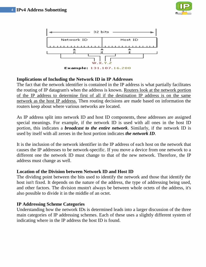
4 IPv4 Address Subnetting
Implications of Including the Network ID in IP Addresses The fact that the network identifier is contained in the IP address is what partially facilitates
the routing of IP datagram's when the address is known. Routers look at the network portion
of the IP address to determine first of all if the destination IP address is on the same
network as the host IP address. Then routing decisions are made based on information the
routers keep about where various networks are located.
As IP address split into network ID and host ID components, these addresses are assigned
special meanings. For example, if the network ID is used with all ones in the host ID
portion, this indicates a broadcast to the entire network. Similarly, if the network ID is
used by itself with all zeroes in the host portion indicates the network ID.
It is the inclusion of the network identifier in the IP address of each host on the network that
causes the IP addresses to be network-specific. If you move a device from one network to a
different one the network ID must change to that of the new network. Therefore, the IP
address must change as well.
Location of the Division between Network ID and Host ID The dividing point between the bits used to identify the network and those that identify the
host isn't fixed. It depends on the nature of the address, the type of addressing being used,
and other factors. The division mustn't always be between whole octets of the address, it's
also possible to divide it in the middle of an octet.
IP Addressing Scheme Categories Understanding how the network IDs is determined leads into a larger discussion of the three
main categories of IP addressing schemes. Each of these uses a slightly different system of
indicating where in the IP address the host ID is found.
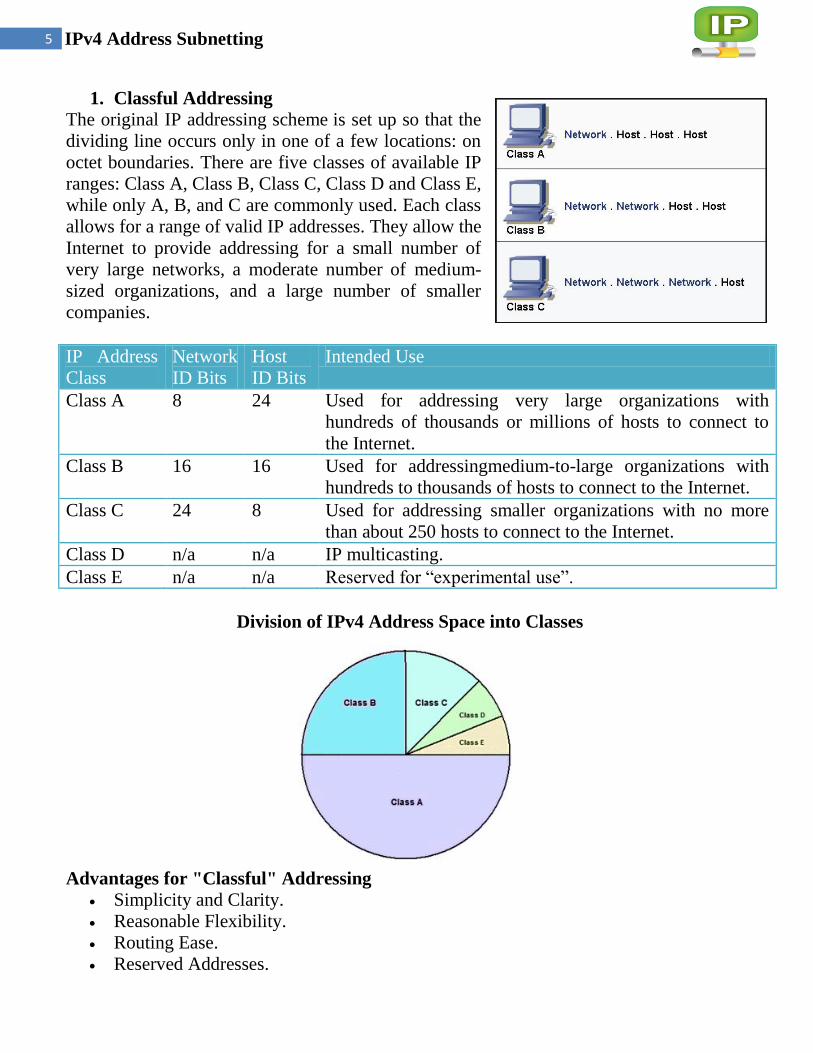
5 IPv4 Address Subnetting
1. Classful Addressing
The original IP addressing scheme is set up so that the
dividing line occurs only in one of a few locations: on
octet boundaries. There are five classes of available IP
ranges: Class A, Class B, Class C, Class D and Class E,
while only A, B, and C are commonly used. Each class
allows for a range of valid IP addresses. They allow the
Internet to provide addressing for a small number of
very large networks, a moderate number of medium-
sized organizations, and a large number of smaller
companies.
IP Address
Class
Network
ID Bits
Host
ID Bits
Intended Use
Class A 8 24 Used for addressing very large organizations with
hundreds of thousands or millions of hosts to connect to
the Internet.
Class B 16 16 Used for addressingmedium-to-large organizations with
hundreds to thousands of hosts to connect to the Internet.
Class C 24 8 Used for addressing smaller organizations with no more
than about 250 hosts to connect to the Internet.
Class D n/a n/a IP multicasting.
Class E n/a n/a Reserved for “experimental use”.
Division of IPv4 Address Space into Classes
Advantages for "Classful" Addressing
Simplicity and Clarity.
Reasonable Flexibility.
Routing Ease.
Reserved Addresses.

6 IPv4 Address Subnetting
Determining Address Class from the First Octet Bit Pattern As humans we generally work with addresses in dotted decimal notation and not in binary,
but it's pretty easy to see the ranges that correspond to the classes.
One of the benefits of the relatively simple “Classful” scheme is that information about the
classes is encoded directly into the IP address. This means we can determine in advance
which address ranges belong to each class, and the opposite is possible: we can identify
which class is associated with any address by examining just a few bits of the address. For
example, consider class B. The first two bits of the first octet are “10”. The remaining bits
can be any combination of ones and zeroes.
IP
Address
Class
Lowest
Binary Value
of First Octet
Highest
Binary Value
of First Octet
Range of First
Octet Decimal
Values
Theoretical IP Address Range
Class A 0000 0001 0111 1110 1 to 126 1.0.0.0 to126.255.255.255
Class B 1000 0000 1011 1111 128 to 191 128.0.0.0 to191.255.255.255
Class C 1100 0000 1101 1111 192 to 223 192.0.0.0 to223.255.255.255
Class D 1110 0000 1110 1111 224 to 239 224.0.0.0 to 239.255.255.255
Class E 1111 0000 1111 1111 240 to 255 240.0.0.0 to 255.255.255.255
IP Address Class A, B and C Network and Host Capacities Classes A, B and C are the ones actually assigned for normal (unicast) addressing purposes
on IP internetworks. They differ in the number of bits (and octets) used for the network ID
compared to the host ID. The number of different networks possible in each class is a
function of the number of bits assigned to the network ID, and likewise, the number of hosts
possible in each network depends on the number of bits provided for the host ID.
Based on this information, we can calculate the number of networks in each class, and for
each class, the number of host IDs per network.

7 IPv4 Address Subnetting
IP Address
Class
Network ID Bits/
Host IDBits
First Octet of
IP Address
Number of Possible
Network IDs
# Of Host IDs Per
Network ID
Class A 8 / 24 0xxx xxxx 28 = 256 2
24-2 = 16,277,214
Class B 16 / 16 10xx xxxx 216
= 65,536 216
-2 = 65,534
Class C 24 / 8 110x xxxx 224
=16,277,216 28-2 = 254
IP Addresses with Special Meanings
Most IP addresses have the “usual” meaning: they refer to an interface to a device on a
TCP/IP network. However, some IP addresses do not refer directly to specific hardware
devices in this manner. Instead, they are used to refer “indirectly” to one or more devices.
Special Address Patterns Special IP addresses are constructed by replacing the normal host ID in an IP address with
one of two special patterns. The two patterns are:
o All Zeroes: When the host bits are replaced by a set of all zeroes, the special meaning is
the equivalent of the Network ID that represent all hosts in that network especially in
the routing table.
o All Ones: When the host bits are replaced by a set of all ones, this has the special
meaning of the broadcast ID of the network, this address used to send a common
message for all hosts exists in this network.
IP Reserved, Loopback and Private Addresses
In addition to these unusable special meaning numbers, there are several other sets of IP
addresses set aside for various special uses, which are not available for normal address
assignment. These ranges of IP addresses generally fall into the following three categories:
reserved, loopback and private addresses.
Reserved Addresses
Several blocks of addresses were designated just as “reserved” with no specific indication
given of what they were reserved for. They may have been set aside for future
experimentation, or for internal use in managing the Internet, or for other purposes. These
address extract along 0.0.0.0 class and 255.0.0.0 class.
Loopback Addresses
Normally, when a TCP/IP application wants to send information, that information travels
down the protocol layers to IP where it is encapsulated in an IP datagram. That datagram
then passes down to the data link layer of the device's physical network for transmission to
the next hop, on the way to the IP destination.
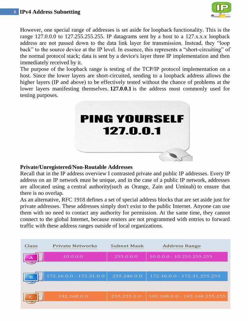
8 IPv4 Address Subnetting
However, one special range of addresses is set aside for loopback functionality. This is the
range 127.0.0.0 to 127.255.255.255. IP datagrams sent by a host to a 127.x.x.x loopback
address are not passed down to the data link layer for transmission. Instead, they “loop
back” to the source device at the IP level. In essence, this represents a “short-circuiting” of
the normal protocol stack; data is sent by a device's layer three IP implementation and then
immediately received by it.
The purpose of the loopback range is testing of the TCP/IP protocol implementation on a
host. Since the lower layers are short-circuited, sending to a loopback address allows the
higher layers (IP and above) to be effectively tested without the chance of problems at the
lower layers manifesting themselves. 127.0.0.1 is the address most commonly used for
testing purposes.
Private/Unregistered/Non-Routable Addresses Recall that in the IP address overview I contrasted private and public IP addresses. Every IP
address on an IP network must be unique, and in the case of a public IP network, addresses
are allocated using a central authority(such as Orange, Zain and Uminah) to ensure that
there is no overlap.
As an alternative, RFC 1918 defines a set of special address blocks that are set aside just for
private addresses. These addresses simply don't exist to the public Internet. Anyone can use
them with no need to contact any authority for permission. At the same time, they cannot
connect to the global Internet, because routers are not programmed with entries to forward
traffic with these address ranges outside of local organizations.
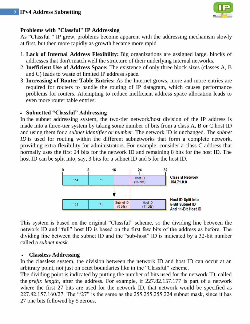
9 IPv4 Address Subnetting
Problems with "Classful" IP Addressing
As “Classful “ IP grew, problems become apparent with the addressing mechanism slowly
at first, but then more rapidly as growth became more rapid
1. Lack of Internal Address Flexibility: Big organizations are assigned large, blocks of
addresses that don't match well the structure of their underlying internal networks.
2. Inefficient Use of Address Space: The existence of only three block sizes (classes A, B
and C) leads to waste of limited IP address space.
3. Increasing of Router Table Entries: As the Internet grows, more and more entries are
required for routers to handle the routing of IP datagram, which causes performance
problems for routers. Attempting to reduce inefficient address space allocation leads to
even more router table entries.
Subnetted “Classful” Addressing
In the subnet addressing system, the two-tier network/host division of the IP address is
made into a three-tier system by taking some number of bits from a class A, B or C host ID
and using them for a subnet identifier or number. The network ID is unchanged. The subnet
ID is used for routing within the different subnetworks that form a complete network,
providing extra flexibility for administrators. For example, consider a class C address that
normally uses the first 24 bits for the network ID and remaining 8 bits for the host ID. The
host ID can be split into, say, 3 bits for a subnet ID and 5 for the host ID.
This system is based on the original “Classful” scheme, so the dividing line between the
network ID and “full” host ID is based on the first few bits of the address as before. The
dividing line between the subnet ID and the “sub-host” ID is indicated by a 32-bit number
called a subnet mask.
Classless Addressing
In the classless system, the division between the network ID and host ID can occur at an
arbitrary point, not just on octet boundaries like in the “Classful” scheme.
The dividing point is indicated by putting the number of bits used for the network ID, called
the prefix length, after the address. For example, if 227.82.157.177 is part of a network
where the first 27 bits are used for the network ID, that network would be specified as
227.82.157.160/27. The “/27” is the same as the 255.255.255.224 subnet mask, since it has
27 one bits followed by 5 zeroes.

10 IPv4 Address Subnetting
IP Address Adjuncts: Subnet Mask and Default Gateway
The original “Classful” scheme the division between network ID and host ID is implied.
However, if either Subnetting or classless addressing is used, then the subnet mask or “slash
number” are required to fully qualify the address. These numbers are considered adjuncts to
the IP address and usually mentioned as the address itself, because without them, it is not
possible to know where the network ID ends and the host ID begins.
One other number that is often specified along with the IP address for a device is the default
gateway identifier. In simplest terms, this is the IP address of the router that provides
default routing functions for a particular device. When a device on an IP network wants to
send a datagram to a device it can't see on its local IP network, it sends it to the default
gateway which takes care of routing functions. Without this, each IP device would also
have to have knowledge of routing functions and routes, which would be inefficient.
IP Subnet Addressing ("Subnetting") Concepts
The original “Classful” IP addressing scheme conceptually divides a large internetwork into
a simple two-level hierarchy: many networks of different sizes, each of which contains a
number of hosts. The system works well for smaller organizations that may connect all their
machines in a single network. However, it lacks flexibility for large organizations that often
have many subnetworks, or subnets. To better meet the administrative and technical
requirements of larger organizations, the “Classful” IP addressing system was enhanced
through a technique known as subnet addressing, or Subnetting.
IP Subnet Addressing Overview, Motivation, and Advantages
IP addressing was originally designed around the assumption of a strict two-level hierarchy
for internetworks. The first level was the network, and the second level the host. Each
organization was usually represented by a single network identifier that indicated a Class A,
B or C block dedicated to them. Within that network they had to put all of the devices they
wanted to connect to the public IP network. The original “Classful” addressing scheme,
there was no good solution to address a big company with thousands of computers and
devices on one big physical network!
The basic idea behind subnet addressing is to add an additional hierarchical level in the way
IP addresses are interpreted. The concept of a network remains unchanged, but instead of
having just “hosts” within a network, a new two-level hierarchy is created: subnets and
hosts. Each subnet is a subnetwork, and functions much the way a full network does in
conventional Classful addressing. A three-level hierarchy is thus created: networks, which
contain subnets, each of which then has a number of hosts.
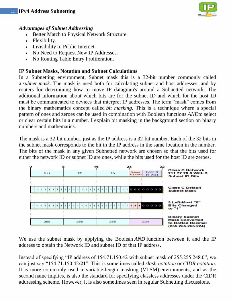
11 IPv4 Address Subnetting
Advantages of Subnet Addressing Better Match to Physical Network Structure.
Flexibility.
Invisibility to Public Internet.
No Need to Request New IP Addresses.
No Routing Table Entry Proliferation.
IP Subnet Masks, Notation and Subnet Calculations
In a Subnetting environment, Subnet mask this is a 32-bit number commonly called
a subnet mask. The mask is used both for calculating subnet and host addresses, and by
routers for determining how to move IP datagram's around a Subnetted network. The
additional information about which bits are for the subnet ID and which for the host ID
must be communicated to devices that interpret IP addresses. The term “mask” comes from
the binary mathematics concept called bit masking. This is a technique where a special
pattern of ones and zeroes can be used in combination with Boolean functions ANDto select
or clear certain bits in a number. I explain bit masking in the background section on binary
numbers and mathematics.
The mask is a 32-bit number, just as the IP address is a 32-bit number. Each of the 32 bits in
the subnet mask corresponds to the bit in the IP address in the same location in the number.
The bits of the mask in any given Subnetted network are chosen so that the bits used for
either the network ID or subnet ID are ones, while the bits used for the host ID are zeroes.
We use the subnet mask by applying the Boolean AND function between it and the IP
address to obtain the Network ID and subnet ID of that IP address.
Instead of specifying “IP address of 154.71.150.42 with subnet mask of 255.255.248.0”, we
can just say “154.71.150.42/21”. This is sometimes called slash notation or CIDR notation.
It is more commonly used in variable-length masking (VLSM) environments, and as the
second name implies, is also the standard for specifying classless addresses under the CIDR
addressing scheme. However, it is also sometimes seen in regular Subnetting discussions.

12 IPv4 Address Subnetting
IP Default Subnet Masks for Address Classes A, B and C
Just as is always the case, the subnet mask for a default, unsubnetted class A, B or C
network has ones for each bit that is used for network ID or subnet ID, and zeroes for the
host ID bits. This is called the default subnet mask for each of the IP address classes. This
default subnet masks will always have 255s or 0s when expressed in decimal notation.
IP
Address
Class
Network ID
bits / Host ID
bits
Default Subnet Mask
First Octet Second Octet Third Octet Fourth Octet
Class A 8 / 24 11111111(255) 00000000(0) 00000000(0) 00000000(0)
Class B 16 / 16 11111111(255) 11111111(255) 00000000(0) 00000000(0)
Class C 24 / 8 11111111(255) 11111111(255) 11111111(255) 00000000(0)
Deciding How Many Subnet Bits to Use
The key decision in Subnetting is how many bits to take from the host ID portion of the IP
address to put into the subnet ID. The number of subnets possible on our network is two to
the power of the number of bits we use to express the subnet ID, and the number of hosts
possible per subnet is two to the power of the number of bits left in the host ID (less two,
which I will explain later in this topic).
Thus, the decision of how many bits to use for each of the subnet ID and host ID represents
a fundamental trade-off in subnet addressing:
o Each bit taken from the host ID for the subnet ID doubles the number of subnets that are
possible in the network.
o Each bit taken from the host ID for the subnet ID (approximately) halves the number of
hosts that are possible within each subnet on the network.

13 IPv4 Address Subnetting
Trading Off Bit Allocations to Meet Subnetting Requirements This is the key design decision in Subnetting is how to divide the “Classful” host ID into
subnet ID and host ID bits. We must make this choice based on our requirements for the
number of subnets that exist in the network, and also on the maximum number of hosts that
need to be assigned to each subnet in the network.
The number of hosts allowed in each subnet is the binary power of the number of host ID
bits remaining after Subnetting, less two. The reduction by two occurs because the all-
zeroes and all-ones host IDs within each subnet are reserved for two “special meaning”
addresses: to refer to the sub network itself and its local broadcast address. In some
implementations, the number of subnets is also reduced by two because the all-zeroes and
all-ones subnet IDs were originally not allowed to be used.
IP Subnetting Summary Tables For Class A, Class B and Class C Networks
Since there are only a few options for how to subnet each of Class A, Class B and Class C
networks, Three tables have been listed for each class These tables can help you
quickly decide how many bits to use for subnet ID and host ID, and then what the subnet
mask is for their selection.

Class A
# of Subnet
ID Bit
# of Host
ID Bits
Subnets Per
Network
# of Hosts
Per Subnet
Subnet Mask(Binary / Dotted Decimal) Subnet Mask
CIDR
0 24 1 16,277,214 11111111.00000000.0000000.00000000 (255.0.0.0) /8
1 23 2 8,388,606 11111111.10000000.0000000.00000000 (255.128.0.0) /9
2 22 4 4,194,302 11111111.11000000.0000000.00000000 (255.192.0.0) /10
3 21 8 2,097,150 11111111.11100000.00000000.00000000 (255.224.0.0) /11
4 20 16 1,048,574 11111111.11110000.00000000.00000000 (255.240.0.0) /12
5 19 32 524,286 11111111.11111000.00000000.00000000 (255.248.0.0) /13
6 18 64 262,142 11111111.11111100.00000000.00000000 (255.252.0.0) /14
7 17 128 131,070 11111111.11111110.00000000.00000000 (255.254.0.0) /15
8 16 256 65,534 11111111.11111111.00000000.00000000(255.255.0.0) /16
9 15 512 32,766 11111111.11111111.10000000.00000000 (255.255.128.0) /17
10 14 1,024 16,382 11111111.11111111.11000000.00000000 (255.255.192.0) /18
11 13 2,048 8,190 11111111.11111111.11100000.00000000 (255.255.224.0) /19
12 12 4,096 4,094 11111111.11111111.11110000.00000000 (255.255.240.0) /20
13 11 8,192 2,046 11111111.11111111.11111000.00000000(255.255.248.0) /21
14 10 16,384 1,022 11111111.11111111.11111100.00000000 (255.255.252.0) /22
15 9 32,768 510 11111111.11111111.11111110.00000000 (255.255.254.0) /23
16 8 65,536 254 11111111.11111111.11111111.00000000 (255.255.255.0) /24
17 7 131,072 126 11111111.11111111.11111111.10000000(255.255.255.128) /25
18 6 262,144 62 11111111.11111111.11111111.11000000(255.255.255.192) /26
19 5 524,288 30 11111111.11111111.11111111.11100000(255.255.255.224) /27
20 4 1,048,576 14 11111111.11111111.11111111.11110000(255.255.255.240) /28
21 3 2,097,152 6 11111111.11111111.11111111.11111000(255.255.255.248) /29
22 2 4,194,304 2 11111111.11111111.11111111.11111100(255.255.255.252) /30

15 IPv4 Address Subnetting
Class B
# of
Subnet
ID Bit
# of
Host ID
Bits
# of Subnets
Per Network
# of Hosts
Per Subnet
Subnet Mask(Binary / Dotted Decimal) Subnet
Mask
CIDR
0 16 1 65,534 11111111.11111111.00000000.00000000 (255.255.0.0) /16
1 15 2 32,766 11111111.11111111.10000000.00000000(255.255.128.0) /17
2 14 4 16,382 11111111.11111111.11000000.00000000 (255.255.192.0) /18
3 13 8 8,190 11111111.11111111.11100000.00000000 (255.255.224.0) /19
4 12 16 4,094 11111111.11111111.11110000.00000000 (255.255.240.0) /20
5 11 32 2,046 11111111.11111111.11111000.00000000(255.255.248.0) /21
6 10 64 1,022 11111111.11111111.11111100.00000000 (255.255.252.0) /22
7 9 128 510 11111111.11111111.11111110.00000000(255.255.254.0) /23
8 8 256 254 11111111.11111111.11111111.00000000 (255.255.255.0) /24
9 7 512 126 11111111.11111111.11111111.10000000 (255.255.255.128) /25
10 6 1,024 62 11111111.11111111.11111111.11000000 (255.255.255.192) /26
11 5 2,048 30 11111111.11111111.11111111.11100000 (255.255.255.224) /27
12 4 4,096 14 11111111.11111111.11111111.11110000 (255.255.255.240) /28
13 3 8,192 6 11111111.11111111.11111111.11111000 (255.255.255.248) /29
14 2 16,384 2 11111111.11111111.11111111.11111100 (255.255.255.252) /30
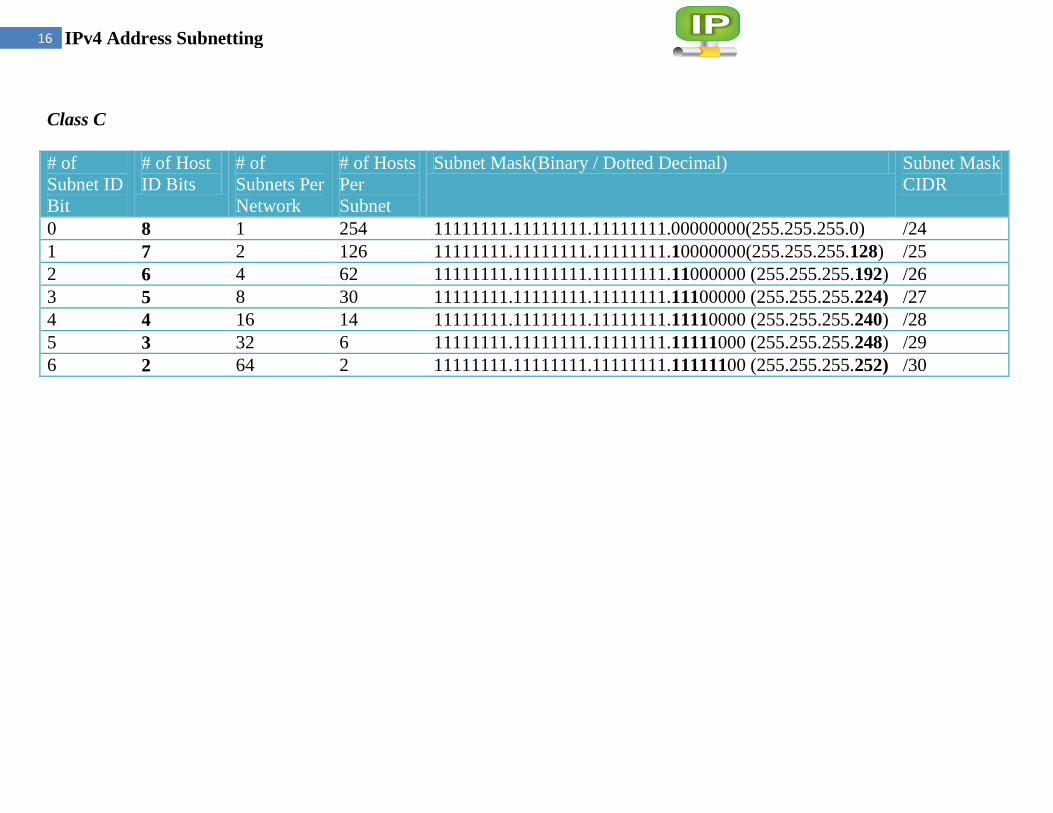
16 IPv4 Address Subnetting
Class C
# of
Subnet ID
Bit
# of Host
ID Bits
# of
Subnets Per
Network
# of Hosts
Per
Subnet
Subnet Mask(Binary / Dotted Decimal) Subnet Mask
CIDR
0 8 1 254 11111111.11111111.11111111.00000000(255.255.255.0) /24
1 7 2 126 11111111.11111111.11111111.10000000(255.255.255.128) /25
2 6 4 62 11111111.11111111.11111111.11000000 (255.255.255.192) /26
3 5 8 30 11111111.11111111.11111111.11100000 (255.255.255.224) /27
4 4 16 14 11111111.11111111.11111111.11110000 (255.255.255.240) /28
5 3 32 6 11111111.11111111.11111111.11111000 (255.255.255.248) /29
6 2 64 2 11111111.11111111.11111111.11111100 (255.255.255.252) /30

University of Jordan
Faculty of Engineering & Technology
Computer Engineering Department
Computer Networks Laboratory
907528
VLSM & Route Summarization

2 VLSM & Route Summarization
IP Variable Length Subnet Masking (VLSM)
Normal Subnet masking replaces the two-level IP addressing scheme with a more flexible
three-level method. Since it lets network administrators assign IP addresses to hosts based on
how they are connected in physical networks, subnetting is a real breakthrough for those
maintaining large IP networks. It has its own weaknesses though, and still has room for
improvement. The main weakness of normal subnetting is in fact that the subnet ID
represents only one additional hierarchical level in how IP addresses are interpreted and used
for routing.
The Problem with Single-Level Subnetting
In large networks, the need to divide our entire network into only one level of subnetworks
doesn't represent the best use of our IP address block. Furthermore, we have already seen that
since the subnet ID is the same length throughout the network, we can have problems if we
have subnetworks with very different numbers of hosts on them—the subnet ID must be
chosen based on whichever subnet has the greatest number of hosts, even if most of subnets
have far fewer.
This is inefficient even in small networks, and can result in the need to use extra addressing
blocks while wasting many of the addresses in each block.
The Solution: Variable Length Subnet Masking The solution to this situation is an enhancement to the basic subnet addressing scheme
called Variable Length Subnet Masking (VLSM). VLSM seems complicated at first, but is
easy to comprehend if you understand basic subnetting. The idea is that you subnet the
network, and then subnet the subnets just the way you originally subnetted the network. In
fact, you can do this multiple times, creating subnets of subnets of subnets, as many times as
you need (subject to how many bits you have in the host ID of your address block). It is
possible to choose to apply this multiple-level splitting to only some of the subnets, allowing
you to selectively cut the "IP address pie" so that some of the slices are bigger than others.

3 VLSM & Route Summarization
Multiple-Level Subnetting Using VLSM VLSM subnetting is done the same way as regular subnetting; it is just more complex
because of the extra levels of subnetting hierarchy. You do an initial subnetting of the
network into large subnets, and then further break down one or more of the subnets as
required. You add bits to the subnet mask for each of the "sub-subnets" and "sub-sub-
subnets" to reflect their smaller size. In VLSM, the slash notation of classless addressing is
commonly used instead of binary subnet masks
4 VLSM & Route Summarization
Let's take about the example above again and see how we can make everything fit using
VLSM. We start with our Class C network, 201.45.222.0/24. We then do three subnetting as
follows we first do initial subnetting by using one bit for the subnet ID, leaving us 7 bits for
the host ID. This gives us two subnets: 201.45.222.0/25 and 201.45.222.128/25. Each of
these can have a maximum of 126 hosts. We set aside the first of these for subnet S6 and its
100 hosts.
We take the second subnet, 201.45.222.128/25, and subnet it further into two sub-subnets.
We do this by taking one bit from the 7 bits left in the host ID. This gives us the sub-subnets
201.45.222.128/26 and 201.45.222.192/26, each of which can have 62 hosts. We set aside
the first of these for subnet S5 and its 50 hosts.
We take the second sub-subnet, 201.45.222.192/26, and subnet it further into four sub-sub-
subnets. We take 2 bits from the 6 that are left in the host ID. This gives us four sub-sub-
subnets that each can have a maximum of 14 hosts. These are used for S1, S2, S3 and S4.
VLSM greatly improves both the flexibility and the efficiency of subnetting. In order to use
it, routers that support VLSM-capable routing protocols must be employed. VLSM also
requires more care in how routing tables are constructed to ensure that there is no ambiguity
in how to interpret an address in the network.
IP Subnetting: Practical Subnet Design and Address Determination Example
This section divides subnetting into five relatively straight-forward stages that cover
determining requirements, making the design decision of how many bits to use for subnet ID
and host ID, and then determining important numbers such as the subnet mask, subnet
addresses and host addresses.
My focus in this section is on showing the practical “how” of subnetting. The topics here
work through two examples using a Class B and a Class C sample network to show you how
subnetting is done.
IP Subnetting Step #1: Requirements Analysis
When you are building or upgrading a network as a whole, the first step isn't buying
hardware, or figuring out protocols, or even design,its requirements analysis, the process of
determining what it is the network needs to do. Without this foundation, you risk
implementing a network that may perfectly match your design but not meet the needs of your
organization.

5 VLSM & Route Summarization
Analyzing the requirements of the network for subnetting isn't difficult, because there are
only a few issues that we need to consider. Since requirements analysis is usually done by
asking questions, here's a list of the most important questions in analyzing subnetting
requirements:
What class is our IP address block?
How many physical subnets are on the network? (A “physical subnet” generally refers to a
broadcast domain on a LAN; a set of hosts on a physical network bounded by routers.)
Do we adding any more physical networks in the near future, and if so, how many?
How many hosts do we have in the largest of our subnets today?
How many hosts do we having in the largest subnet in the near future?
We need to analyze the requirements above not only for the present network, but for the near
future as well. The current values for these two numbers represent how the network needs to
be designed today. However, designing only for the present is not a good idea. The term
“near future” is necessarily because it depends on how far into the future the organization
wants to look. On the one hand, planning for several years' growth can make sense, if you
have enough IP addresses to do it. On the other, you don't want to plan too far out, since
changes in the short term may cause you to completely redesign your network anyway.
IP Subnetting Step #2: Partitioning Network Address Host Bits
after we complete our brief requirements analysis, we should know the two critical
parameters that we must have in order to subnet our network: the number of subnets required
for the network, and the maximum number of hosts per subnetwork. In using these two
figures to design our Subnetted network, we will be faced with the key design decision in
subnetting: how to divide the 8, 16 or 24 bits in the “classful” host ID into subnet ID and host
ID.
We need to decide how many bits to borrow from the host ID to use for the subnet ID. The
fundamental trade-off in choosing this number is as follows:
Each bit taken from the host ID for the subnet ID doubles the number of subnets that are
possible in the network.
Each bit taken from the host ID for the subnet ID (approximately) halves the number of
hosts that are possible within each subnet on the network.
There are six possible ways this decision can be made for a Class C network, as the
following figure.

6 VLSM & Route Summarization
The relationship between the bits and the number of subnets and hosts is as follows:
o The number of subnets allowed in the network is two to the power of the number of subnet
ID bits.
o The number of hosts allowed per subnet is two to the power of the number of host ID bits,
less two.
We subtract two from the number of hosts in each subnet to exclude the “special meaning”
cases where the host ID is all zeroes or all ones. First we must calculate the number of
subnets and hosts when we use the subnet ID bits and leave the rest for the host ID.
Class B Subnetting Design Example In some cases, especially with larger networks, we may have multiple choices. Consider the
following example, the larger Class B network 166.113.0.0, where we have a total of 15
subnets and the largest has 450 hosts.

7 VLSM & Route Summarization
IP Subnetting Step #3: Determining the Custom Subnet Mask
Once we have decided how many bits to use for the subnet ID and how many to leave for the
host ID, we can determine the custom subnet mask for our network.
Calculating the Custom Subnet Mask
We determine the subnet mask in binary form from the information we already have about
our network, and then convert the mask to decimal. To refresh your memory and guide the
process, remember this: the subnet mask is a 32-bit binary number where a 1 represents each
bit that is part of the network ID or subnet ID, and a 0 represents each bit of the host ID.
Class C Custom Subnet Mask Calculation Example
Refer back to the Class C example in the previous topic. We decided to use 3 bits for the
subnet ID, leaving 5 bits for the host ID. Here are the steps we will follow to determine the
custom subnet mask for this network.
1. Determine Default Subnet Mask: Each of Classes A, B and C has a default subnet
mask, which is the subnet mask for the network prior to subnetting. It has a 1 for each
network ID bit and a 0 for each host ID bit. For Class C, the subnet mask is
255.255.255.0.
2. Change Left-Most Zeroes to Ones for Subnet Bits: We have decided to use 3 bits
for the subnet ID. The subnet mask has to have a 1 for each of the network ID or
subnet ID bits. The network ID bits are already 1 from the default subnet mask, so, we
change the 3 left-most 0 bits in the default subnet mask from a 0 to 1
3. Convert Subnet Mask To Dotted Decimal Notation: We take each of the octets in
the subnet mask and convert it to decimal. The result is our custom subnet mask in the
form we usually see it: 255.255.255.224.
4. Express Subnet Mask In “Slash Notation”: Alternately, we can express the subnet
mask in “slash notation”. This is just a slash followed by the number of ones in the
subnet mask. 255.255.255.224 is equivalent to “/27”.

8 VLSM & Route Summarization
Class B Custom Subnet Mask Calculation Example Now, let's do the same example with our Class B network (166.113.0.0) with 5 bits for the
subnet ID (with a bit less narration this time):
1. Determine Default Subnet Mask: For Class B, the subnet mask is 255.255.0.0. In
binary, this is:11111111 11111111 00000000 00000000
2. Change Left-Most Zeroes To Ones For Subnet Bits: We have decided to use 5 bits
for the subnet ID, so, we change the 5 left-most 0 bits from a 0 to 1
3. Convert Subnet Mask To Dotted Decimal Notation: We take each of the octets in
the subnet mask and convert it to decimal, to give us a custom subnet mask of
255.255.248.0
4. Express Subnet Mask In “Slash Notation”: We can express the subnet mask
255.255.248.0 as “/21”, since it is 21 ones followed by 11 zeroes. In other words, its
prefix length is 21.
IP Subnetting Step #4: Determining Subnet Identifiers and Subnet Addresses:
The network ID assigned to our network applies to the entire network. This includes all
subnets and all hosts in all subnets. Each subnet, however, needs to be identified with a
unique subnet identifier calledsubnet ID, so it can be differentiated from the other subnets in
the network. This is of course the purpose of the subnet ID bits that we took from the host ID
bits in subnetting. After we have identified each subnet we need to determine the address of
each subnet, so we can use this in assigning hosts specific IP addresses.
The key to understanding how to determine subnet IDs and subnet addresses is to always
work in binary form, and then convert to decimal later. We determine the subnet IDs and
addresses as follows
1. Subnet ID: This is just the subnet number, and can be expressed in either binary or
decimal form.

9 VLSM & Route Summarization
2. Subnet Address: This is the address formed by taking the address of the network as a
whole, and substituting the (binary) subnet ID in for the subnet ID bits. We need to do this
in binary, but only for the octets where there are subnet ID bits; the ones where there are
only network ID bits or only host ID bits are left alone.
Class C Subnet ID and Address Determination Example
This diagram shows each of the 8 possible subnets created when we use 3 bits for the subnet
ID in a Class C network. The binary subnet ID is simply substituted for the subnet bits, and
the resulting 32-bit number converted to dotted decimal form. The address of any subnet can
be found by adding 32 to the last octet of the previous subnet. This pattern occurs for all
subnetting choices; the increment depends on how many bits we are using for the subnet ID.

10 VLSM & Route Summarization
Here, the increment is 32, which is 25; 5 is the number of host ID bits left after we took 3
subnet ID bits.
Class B Subnet ID and Address Determination Example Class B network 166.113.0.0. We are using 5 bits for the subnet ID, leaving 11 hosts ID bits.
IP Subnetting Step #5: Determining Host Addresses for Each Subnet
Once we know the addresses of each of the subnets in our network, we use these addresses as
the basis for assigning IP addresses to the individual hosts in each subnet. We start by
associating a subnet base address with each physical network (since at least in theory, our
subnets correspond to our physical networks). We then sequentially assign hosts particular IP
addresses within the subnet (or in a different manner, if we prefer!)
Determining host addresses is really quite simple, once we know the subnet address. All we
do is substitute the numbers 1, 2, 3… and so on for the host ID bits in the subnet address.

11 VLSM & Route Summarization
Class C Host Address Determination Example
Let's start with our Class C example again, 211.77.20.0, which we divided into 8 subnets
using 3 subnet bits.
This diagram shows how both subnet addresses and host addresses are determined in a two-
step process. The subnet addresses are found by substituting subnet ID values (shown in red)
for the subnet ID bits of the network. Then, for any given subnet address, we can determine a
host address by substituting a host number (shown in blue) for the host ID bits within that
subnet. So, for example, host #2 in subnet #6 has “110” for the subnet ID and “00010” for
the host ID, resulting in a final octet value of “11000010” or 194.
12 VLSM & Route Summarization
"Shortcuts" For Quickly Computing Host Addresses
Defining the host IDs is really quite straight-forward. If you can substitute bits and convert to
decimal, you have all you need to know. You can also see that as was the case with defining
the subnet addresses, there are patterns that you can use in defining host IDs and
understanding how they work. These generally define ways that we can more quickly
determine certain host addresses by working directly in decimal instead of bothering with
binary substitutions. The following are some of the “shortcuts” you can use in determining
host IP addresses in a subnet environment:
o First Host Address: The first host address is always the subnet address with the last octet
incremented by 1. So, in our class C example, subnet #3's base address is 211.77.20.96.
The first host address in subnet #3 is thus 211.77.20.97.
o Subsequent Host Addresses: After you find the first host address, to get the next one you
just add one to the last octet of the previous address. If this makes the last octet 256 (which
can happen only if there are more than 8 host ID bits) you “wrap around” this to zero and
increment the third octet.
o Directly Calculating Host Addresses: If the number of host ID bits is 8 or less, you can
find host #N's address by adding “N” to the last octet's decimal value. For example, in our
class C example, subnet #3's base address is 211.77.20.96. Therefore, host #23 in this
subnet has an address of 211.77.20.119.
If there are more than 8 bits in the host ID, this only works for the first 255 hosts, after
which you have to “wrap around” and increase the value of the third octet. Consider again
subnet #13 in our Class B example, which has a base address of 166.113.104.0. Host #214
on this subnet has address 166.113.104.214, but host #314 isn't 166.113.104.314. It is
166.113.105.58 (host #255 is 166.113.104.255, then host #256 is 166.113.105.0, and we
count up 58 more (314-256) to get to #314, 166.113.105.58).
Range Of Host Addresses:
The range of hosts for any subnet is determined as follows:
First Address: Base address of subnet with last octet incremented by one.
Last Address: Base address of next subnet after this one, less two in the last octet (which
may require changing a “0” in the last octet to “254” and reducing the value of the third
octet by 1).
Broadcast Address: The broadcast address for a subnet is always one less than the base
address of the subsequent subnet. Or alternately, one more than the last “real” host address
of the subnet. So, for subnet #17 in our Class B example, the broadcast address is
166.113.143.255.
13 VLSM & Route Summarization
Important note about subnetting:
The network ID is the same for all hosts in all subnets, and all subnets in the network.
The subnet ID is the same for all hosts in each subnet, but unique to each subnet in the
network.
The host ID is unique within each subnet. Each subnet has the same set of host IDs.
IP Classless Addressing: Classless Inter-Domain Routing (CIDR) / "Supernetting"
As the early Internet began to grow dramatically, three main problems arose with the original
“classful” addressing scheme. These difficulties were addressed partially through subnet
addressing, which provides more flexibility for the administrators of individual networks on
an internet. Subnetting doesn't really tackle the problems in general terms. Some of these
issues remain due to the use of classes even with subnets.
In order to extend the life of IP version 4 until the newer IP version 6 could be completed, it
was necessary to take a new approach to addressing IPv4 devices. This new system calls for
eliminating the notion of address classes entirely, creating a new classless addressing scheme
sometimes called Classless Inter-Domain Routing (CIDR).
A Better Solution: Eliminate Address Classes
It was clear that as long as there were only three sizes of networks, the allocation efficiency
problem could never be properly rectified. The solution was to get rid of the classes
completely, in favor of a classless allocation scheme. This system would solve both of the
main problems with “Classful” addressing: inefficient address space use, and the exponential
growth of routing tables.
The idea behind CIDR is to adapt the concept of subnetting a single network to the entire
internet. In essence, then, classless addressing means that instead of breaking a particular
network into subnets, we can aggregate networks into larger “supernets”. CIDR is sometimes
called Supernetting for this reason: it applies the principles of subnetting to larger networks.
It is this aggregation of networks into supernets that allowed CIDR to resolve the problem of
growing Internet routing tables.
When we are going to apply subnetting concepts to the entire internet, we need to be able to
have subnets of different sizes. After all, that's one of our primary goals in eliminating the
classes. So CIDR is an internet-wide application of not regular one-level subnetting, but
of Variable Length Subnet Masking (VLSM). Just as VLSM lets us split a network as many
times as we want to create subnets, “sub-subnets” and “sub-sub-subnets”, CIDR lets us do
this with the entire Internet, as many times as needed.

14 VLSM & Route Summarization
Benefits of Classless Addressing and Routing:
Efficient Address Space Allocation: Instead of allocating addresses in fixed-size blocks of
low granularity, under CIDR addresses are allocated in sizes of any binary multiple.
Elimination of Class Imbalances: There is no more class A, B and C networks, so there is
no problem with some portions of the address space being widely used while others are
neglected.
Efficient Routing Entries: CIDR's multiple-level hierarchical structure allows a small
number of routing entries to represent a large number of networks. Network descriptions
can be “aggregated” and represented by a single entry. Since CIDR is hierarchical, the
detail of lower-level, smaller networks can be hidden from routers that move traffic
between large groups of networks. This is discussed more completely in the section on IP
routing issues.
No Separate Subnetting Method: CIDR implements the concepts of subnetting within the
internet itself. An organization can use the same method used on the Internet to subdivide
its internal network into subnets of arbitrary complexity without needing a separate
subnetting mechanism.
The Main Disadvantage of CIDR: Complexity
One issue is that it is no longer possible to determine by looking at the first octet to
determine how many bits of an IP address represent the network ID and how many the host
ID. A bit more care needs to be used in setting up routers as well, to make sure that routing is
accomplished correctly.
Classless Inter-Domain Routing (CIDR) Hierarchical Addressing and Notation
With VLSM, we further Subnetted the subnets, taking more bits from the host ID to give us a
multiple-level hierarchy with “sub-subnets”, “sub-sub-subnets” and so forth.
In a classless environment, we completely change how we look at IP addresses, by applying
VLSM concepts not just to one network, but to the entire Internet. In essence, the Internet
becomes just one giant network that is “Subnetted” into a number of large blocks. Some of
these large blocks are then broken down into smaller blocks, which can in turn be broken
down further.
CIDR ("Slash") Notation Just as subnetting required the use of a subnet mask to show which bits belong to the
network ID or subnet ID and which to the host ID, CIDR uses a subnet mask to show where
the line is drawn between host ID and network ID. However, for simplicity, under CIDR we
don't usually work with 32-bit binary subnet masks. Instead, we use slash notation, more
properly called CIDR notation. In this method, we show the size of the network, sometimes
called the prefix length, by following an IP address by an integer that tells us how many bits
are used for the network ID (prefix).

15 VLSM & Route Summarization
For example, consider the network specification 184.13.152.0/22. The “22” means this
network has 22 bits for the network ID and 10 bits for the host ID. This is equivalent to
specifying a network with an address of 184.13.152.0 and a subnet mask of 255.255.252.0.
This sample network provides a total of 1,022 hosts (210
minus 2). The table in the following
topic shows all the different possible network sizes that can be configured under CIDR.
IP Classless Addressing Block Sizes and "Classful" Network Equivalents
The following Table shows each of the possible theoretical ways to divide the 32 bits of an
IP address into network ID and host ID bits under CIDR. For each, the number of hosts in
each network, and the way a network of each size is represented in both slash notation and as
a conventional subnet mask. I have also shown the equivalent number of Class A, Class B
and Class C networks for each.

16 VLSM & Route Summarization
Route Summarization:
The process of advertising a set of addresses as a single address with a less-specific, shorter
subnet mask. Summarization helps reduce the number of entries in routing updates and
lowers the number of entries in local routing tables. It also helps reduce bandwidth utilization
for routing updates and results in faster routing table lookups.
The figure shows a single static route with the address 172.16.0.0 and the mask 255.248.0.0
summarizing all of the 172.16.0.0/16 to 172.23.0.0/16 classful networks. Although
172.22.0.0/16 and 172.23.0.0/16 are not shown in the graphic, these are also included in the
summary route. Notice that the /13 mask (255.248.0.0) is less than the default classful mask
/16 (255.255.0.0). It is possible that a router could have both a specific route entry and a
summary route entry covering the same network.
Calculating Summarized routes:
Summarizing networks into a single address and mask can be done in three steps. Let's look
at the following four networks:
172.20.0.0/16
172.21.0.0/16
172.22.0.0/16
172.23.0.0/16
The second step is to count the number of left-most matching bits to determine the mask for
the summary route. You can see in the figure that the first 14 left-most matching bits match.
This is the prefix, or subnet mask, for the summarized route: /14 or 255.252.0.0.

17 VLSM & Route Summarization
The third step is to copy the matching bits and then add zero bits to determine the
summarized network address. The figure shows that the matching bits with zeros at the end
results in the network address 172.20.0.0. The four networks - 172.20.0.0/16, 172.21.0.0/16,
172.22.0.0/16, and 172.23.0.0/16 - can be summarized into the single network address and
prefix 172.20.0.0/14.

18 VLSM & Route Summarization
Network
ID Bits
Host ID
Bits
Hosts Per
Network
CIDR Equivalent
Subnet Mask
# of “Classful” Networks
Class A Class B Class C
1 31 2,147,483,646 /1 128.0.0.0 128 — —
2 30 1,073,741,822 /2 192.0.0.0 64 — —
3 29 536,870,910 /3 224.0.0.0 32 — —
4 28 268,435,454 /4 240.0.0.0 16 — —
5 27 134,217,726 /5 248.0.0.0 8 — —
6 26 67,108,862 /6 252.0.0.0 4 — —
7 25 33,554,430 /7 254.0.0.0 2 — —
8 24 16,777,214 /8 255.0.0.0 1 256 —
9 23 8,388,606 /9 255.128.0.0 ½ 128 —
10 22 4,194,302 /10 255.192.0.0 ¼ 64 —
11 21 2,097,150 /11 255.224.0.0 1/8 32 —
12 20 1,048,574 /12 255.240.0.0 1/16 16 —
13 19 524,286 /13 255.248.0.0 1/32 8 —
14 18 262,142 /14 255.252.0.0 1/64 4 —
15 17 131,070 /15 255.254.0.0 1/128 2 —
16 16 65,534 /16 255.255.0.0 1/256 1 256
17 15 32,766 /17 255.255.128.0 — ½ 128
18 14 16,382 /18 255.255.192.0 — ¼ 64
19 13 8,190 /19 255.255.224.0 — 1/8 32
20 12 4,094 /20 255.255.240.0 — 1/16 16
21 11 2,046 /21 255.255.248.0 — 1/32 8
22 10 1,022 /22 255.255.252.0 — 1/64 4
23 9 510 /23 255.255.254.0 — 1/128 2
24 8 254 /24 255.255.255.0 — 1/256 1
25 7 126 /25 255.255.255.128 — — ½
26 6 62 /26 255.255.255.192 — — ¼
27 5 30 /27 255.255.255.224 — — 1/8
28 4 14 /28 255.255.255.240 — — 1/16
29 3 6 /29 255.255.255.248 — — 1/32
30 2 2 /30 255.255.255.252 — — 1/64

University of Jordan
Faculty of Engineering & Technology
Computer Engineering Department
Computer Networks Laboratory
907528
Static Routing & Default Routes

2 Static Routing & Default Routes
Static Routing: A router can learn about remote networks in one of two ways:
Manually, from configured static routes
Automatically, from a dynamic routing protocol
Static routes Static routes are commonly used when routing from a network to a stub
network. A stub network is a network accessed by a single route. For an example, see the
figure below. Here we see that any network attached to R1 would only have one way to
reach other destinations, whether to networks attached to R2 or to destinations beyond R2.
Therefore, network 172.16.3.0 is a stub network and R1 is a stub router. Running a
routing protocol between R1 and R2 is a waste of resources because R1 has only one way
out for sending non-local traffic. Therefore, static routes are configured for connectivity to
remote networks that are not directly connected to a router. Again, referring to the figure,
we would configure a static route on R2 to the LAN attached to R1. We will also see how
to configure a default static route from R1 to R2 later, so that R1 can send traffic to any
destination beyond R2.
The ip route command The command for configuring a static route is ip route. The complete syntax for
configuring a static route is:
Router(config)#ip route prefix mask {ip-address | interface-type interface-number [ip-
address]} [distance] [name] [permanent] [tag tag]
Most of these parameters are not relevant for our studies. Therefore, we will use a simpler
version of the syntax:
Router(config)#ip route network-address subnet-mask {ip-address | exit-interface }

3 Static Routing & Default Routes
The following parameters are used:
network-address - Destination network address of the remote network to be added to the
routing table
Subnet-mask - Subnet mask of the remote network to be added to the routing table. The
subnet mask can be modified to summarize a group of networks.
One or both of the following parameters must also be used:
ip-address - Commonly referred to as the next-hop router's IP address
Exit-interface - Outgoing interface that would be used in forwarding packets to the
destination network.
Real Life Static Routing Example:
Let's say that you are a network administrator and you just added a new segment to your
network and you've successfully added it to your network's routing tables. Suddenly users
on that segment can't get to a network resource such as an email server, or they can't get
out to the Internet. Static routes are a great quick fix. You can use a static route to get the
users where they need to be, which gives you time to find out what the problem is with the
dynamic routing protocol. Static routes are configured with the ip route command,
followed by the destination network and mask. After that, you must specify either the
next-hop IP address or the local exit interface. Both of the following masks are acceptable:
ip route 172.10.1.0 255.255.255.0 210.1.1.1
ip route 172.10.1.0 255.255.255.0 serial0
Remember, you're specifying either the next-hop router's IP address or the local router's
exit interface!
Default Static Route It is possible that the destination IP address of a packet will match
multiple routes in the routing table. For example, what if we had the following two static
routes in the routing table: 172.16.0.0/24 is Subnetted, 2 subnets S 172.16.1.0 is directly
connected, Serial0/0/0 and S 172.16.0.0/16 is directly connected, Serial0/0/1 Consider a
packet with the destination IP address 172.16.1.10. This IP address matches both routes.
The routing table lookup process will use the most-specific match. Because 24 bits match
the 172.16.1.0/24 route, and only 16 bits of the 172.16.0.0/16 route match, the static route
with the 24 bit match will be used. This is the longest match. The packet will then be
encapsulated in a Layer 2 frame and sent via the Serial 0/0/0 interface. Remember, the
subnet mask in the route entry is what determines how many bits must match the packet's
destination IP address for this route to be a match.
Note: This process is the same for all routes in the routing table including static routes,
routes learned from a routing protocol and directly connected networks.
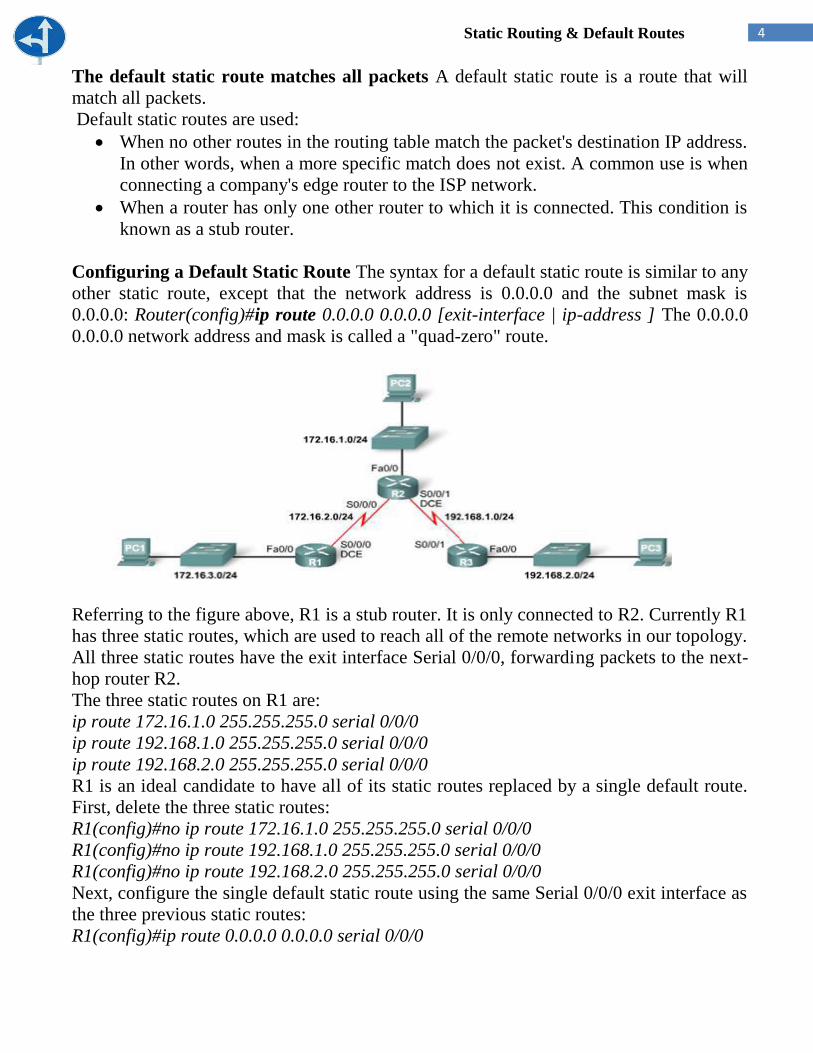
4 Static Routing & Default Routes
The default static route matches all packets A default static route is a route that will
match all packets.
Default static routes are used:
When no other routes in the routing table match the packet's destination IP address.
In other words, when a more specific match does not exist. A common use is when
connecting a company's edge router to the ISP network.
When a router has only one other router to which it is connected. This condition is
known as a stub router.
Configuring a Default Static Route The syntax for a default static route is similar to any
other static route, except that the network address is 0.0.0.0 and the subnet mask is
0.0.0.0: Router(config)#ip route 0.0.0.0 0.0.0.0 [exit-interface | ip-address ] The 0.0.0.0
0.0.0.0 network address and mask is called a "quad-zero" route.
Referring to the figure above, R1 is a stub router. It is only connected to R2. Currently R1
has three static routes, which are used to reach all of the remote networks in our topology.
All three static routes have the exit interface Serial 0/0/0, forwarding packets to the next-
hop router R2.
The three static routes on R1 are:
ip route 172.16.1.0 255.255.255.0 serial 0/0/0
ip route 192.168.1.0 255.255.255.0 serial 0/0/0
ip route 192.168.2.0 255.255.255.0 serial 0/0/0
R1 is an ideal candidate to have all of its static routes replaced by a single default route.
First, delete the three static routes:
R1(config)#no ip route 172.16.1.0 255.255.255.0 serial 0/0/0
R1(config)#no ip route 192.168.1.0 255.255.255.0 serial 0/0/0
R1(config)#no ip route 192.168.2.0 255.255.255.0 serial 0/0/0
Next, configure the single default static route using the same Serial 0/0/0 exit interface as
the three previous static routes:
R1(config)#ip route 0.0.0.0 0.0.0.0 serial 0/0/0

University of Jordan
Faculty of Engineering & Technology
Computer Engineering Department
Computer Networks Laboratory
907528
Distance Vector Routing Protocols

2 Distance Vector Routing Protocols
Fundamentals of Routing Routing is the process of forwarding packets from one network to another; Logical addressing
is used to identify each network as well as each device on the network. The actual movement
of transient traffic through the router is a separate function; it is actually considered to be the
switching function. Routing devices must perform both a routing and a switching function to
be effective.
For a routing decision to take place three major decisions must be made:
1. Is the logical destination addressing a known protocol? Is this protocol enabled on the router
and active?
2. Is the destination logical address in the routing table? If not, discard the packet and send an
ICMP (Internet Control Message Protocol) message to the sender.
3. If the destination logical address is in the routing table, to which interface will the packet be
forwarded? Once this exit, or forwarding interface, is chosen, the router must have an
encapsulation in which to place the packet. This is called framing and is required to forward
the packet to the next-hop logical device.
Once the packet is framed, it is forwarded from hop to hop until it reaches the final destination
device. Routing tables in each device are used to pass the packet to the correct destination
network.
Routing Tables
All the routing information needed for a router to forward packets to a next hop relay device
can be found in the router’s routing table. If a destination logical address is not found in the
table, the router discards the packets. A gateway of last resort can be set on the router to
forward packets not listed in the routing table. This is called setting the default route.
However, this is not a default gateway, nor does it act as a default gateway, so it is important to
not think of setting the gateway of last resort as setting a default gateway. Default gateways are
used on hosts to direct packets to a relay device if the destination logical device is not on the
local segment. Gateway-of-last-resort entries are used to send packets to a next-hop relay
device if the destination logical address is not found in the routing table. If the destination
logical address is in the routing table, then the gateway of last resort will not be used.

3 Distance Vector Routing Protocols
At the top of the routing table are the different codes that describe the entries found in a routing
table. In the example above, the entries include both directly connected static routes and RIP
entries.
Administrative Distances When configuring routing protocols, you need to be aware of administrative distances. These
are used to rate the trustworthiness of routing information received on a router from a neighbor
router. An administrative distance is an integer from 0 to 255, where 0 is the most trusted and
255 means no traffic will be passed via this route.
If a network is directly connected, it will always use the interface connected to the network. If
an administrator configures a static route, the router will believe that route over any other
learned routes.
Packet Switching After a router is started up, the routing protocol tries to establish neighbor relationships in
order to understand the network topology and build the routing table. All routing protocols
perform this differently; for example, some use broadcast addresses to find the neighbors and
some use multicast addresses. Once the neighbors are found, the routing protocol creates a peer
relationship at Layers 4 through 7 of the OSI model. Routing protocols either send periodic
routing updates or exchange Hello messages to maintain the relationship.
Only after the topology is completely understood and the best paths to all remote networks are
decided and put in the routing table can the forwarding of packets begin. This forwarding of
packets received on an interface to an exit interface is known as packet-switching.
Four basic steps for a router to packet switch:
1. The router receives a frame on an interface, runs a CRC (cyclic redundancy check), and
if it is okay, checks the hardware destination address. If it matches, the packet is pulled
from the frame. The frame is discarded and the packet is buffered in main memory.
2. The packet’s destination logical address is checked. This address is looked up in the
routing table for a match. If there is no match, the packet is immediately discarded and
an ICMP message is sent back to the originating device. If there is a match, the packet is
switched to the forwarding interface buffer.
3. The hardware address of the next-hop device must be known. The ARP cache is checked
first and if it is not found, an ARP broadcast is sent to the device. The remote device will
respond with its hardware address.

4 Distance Vector Routing Protocols
4. A new frame is created on that interface and the packet is placed in this frame. The
destination hardware address is the address of the next hop device. Notice that the packet
was not altered in any way.
Dynamic Routing Dynamic routing is the process of using protocols to find and update routing tables on routers
and to maintain a loop-free, single path to each network. This is easier than static or default
routing, but you use it at the expense of router CPU processes and bandwidth usage on the
network links. A routing protocol defines the set of rules used by a router when it
communicates between neighbor routers.
Once the router process knows the metric values of each path, then routing decisions are made.
When a route is learned from different sources, the router will first choose the route with the
lowest administrative distance. If two routes have the same AD, then the router will use the
routing metrics to determine the best path to the remote network. If the AD is the same in both
routes, as well as the metrics, then the routing protocol will load balance.
Routing Protocols There are two classes of dynamic routing protocols:
Distance-vector: the distance-vector protocol uses the distance to a remote network as a
determination of the best path to a remote network. Each time a packet goes through a router,
it’s called a hop. The route with the least number of hops to the remote network is determined
to be the best route. The vector is the determination of direction to the remote network. An
example of a distance-vector protocol is RIP and IGRP. However, not all distance-vector
protocols use hop count in their metric. IGRP uses bandwidth and delay of the line to
determine the best path to a remote network. It is considered a distance-vector protocol because
it sends out the complete routing table at periodic intervals. The periodic routing updates from
a distance-vector router are sent only to directly connected routers and sent as a broadcast of
255.255.255.255. Since the updates include all routes that the sending router knows about, this
is sometimes referred to as “routing by rumor” because a router will accept information from a
neighbor as correct. The disadvantage to distance-vector protocols is that the periodic updates
consume bandwidth even if there are no topology changes to report.

5 Distance Vector Routing Protocols
Link-state: typically called shortest path first, link-state routers create three separate tables.
One of these tables keeps track of directly attached neighbors, one determines the topology of
the entire internetwork, and one is used for the routing table. Link-state routers know more
about the internetwork than any distance-vector protocol. An example of an IP routing protocol
that is completely link-state is OSPF.
To send routing updates, the link-state router uses a triggered-update type of announcement.
These announcements are sent from a router only when a topology change has occurred within
the network. The advantage of link-state routing over distance-vector is that when an update
occurs, only the information about the link that changed is contained in the update.
There is no set way of configuring routing protocols for use with every business. This task is
performed on a case-by-case basis. However, if you understand how the different routing
protocols work, you can make good business decisions.
Distance Vector vs. Link State There are two major differences between Distance Vector routing protocols and Link State
routing protocols.
1. Distance Vector exchanges the routing updates periodically whether the topology is
change or not, this will maximize the convergence time which increases the chance of
routing loops while the Link State routing protocols send triggered change based updates
when there is a topology change. After initial flood, pass small event based triggered
link state updates to all other routers. This will minimize the convergence time that’s
why there is no chance of routing loops.
2. The Distance Vector routing protocols rely on the information from their directly
connected neighbors in order to calculate and accumulate route information. Distance
Vector routing protocols require very little overhead as compared to Link State routing
protocols as measured by memory and processor power while the Link State routing
protocols do not rely solely on the information from the neighbors or adjacent router in
order to calculate route information.

6 Distance Vector Routing Protocols
Instead, Link State routing protocols have a system of databases that they use in order to
calculate the best route to destinations in the network. An extra feature of Link State routing
protocol is that they can detect media types along with other factors. This could increase the
overhead as compare to Distance Vector routing protocols in order to measure by processor
power and memory. Routing Information Protocol (RIP) and Interior Gateway Routing
Protocol (IGRP) are the examples of Distance Vector routing protocols while the Open
Shortest Path First (OSPF) is a classic example of Link State routing protocols.
Other differences of both types of routing protocols are as follows:
Distance Vector
Distance Vector routing protocols are based on Bellman and Ford algorithms.
Distance Vector routing protocols are less scalable such as RIP supports 16 hops and
IGRP has a maximum of 100 hops.
Distance Vector are Classful routing protocols which means that there is no support of
Variable Length Subnet Mask (VLSM) and Classless Inter Domain Routing (CIDR).
Distance Vector routing protocols uses hop count and composite metric.
Common distance vector routing protocols include: RIP, IGRP.
Link State
Link State routing protocols are based on Dijkstra algorithms.
Link State routing protocols are very much scalable supports infinite hops.
Link State routing protocols are classless which means that they support VLSM and
CIDR.
Cost is the metric of the Link State routing protocols.
Link State routing protocols support contiguous subnets.
Metrics When there are multiple routes to the same destination, a router must have a mechanism for
calculating the best path. A metric is a variable assigned to routes as a means of ranking them
from best to worst or from most preferred to least preferred.
Hop Count A hop count metric simply counts router hops. For instance, from router A it is 1 hop to
network 192.168.5.0 if packets are sent out interface 192.168.3.1 (through router B) and 2 hops
if packets are sent out 192.168.1.1 (through routers C and B). Assuming hop count is the only
metric being applied, the best route is the one with the fewest hops, in this case, A-B.
But is the A-B link really the best path? If the A-B link is a DS0 (64 Kbps) link and the A-C
and C-B links are T1 (1.544 Mbps) links, the 2-hop route may actually be best because
bandwidth plays a role in how efficiently traffic travels through the network.
7 Distance Vector Routing Protocols
Bandwidth
A bandwidth metric would choose a higher-bandwidth path over a lower-bandwidth link.
However, bandwidth by itself still may not be a good metric. What if one or both of the T1
links are heavily loaded with other traffic and the 64K link is lightly loaded? Or what if the
higher-bandwidth link also has a higher delay?
Load This metric reflects the amount of traffic utilizing the links along the path. The best path is the
one with the lowest load.
Unlike hop count and bandwidth, the load on a route changes, and therefore the metric will
change. Care must be taken here. If the metric changes too frequently, route flapping—the
frequent alternating between two paths occurs.
Delay Delay is a measure of the time a packet takes to traverse a route. A routing protocol using delay
as a metric would choose the path with the least delay as the best path. There may be many
ways to measure delay. Delay may take into account not only the delay of the links along the
route but also such factors as router latency and queuing delay. On the other hand, the delay of
a route may be not measured at all; it may be a sum of static quantities defined for each
interface along the path. Each individual delay quantity would be an estimate based on the type
of link to which the interface is connected.
Reliability
Reliability measures the likelihood that the link will fail in some way and can be either variable
or fixed. Examples of variable-reliability metrics are the number of times a link has failed or
the number of errors it has received within a certain time period. Fixed-reliability metrics are
based on known qualities of a link as determined by the network administrator. The path with
highest reliability would be selected as best.
Cost This metric is configured by a network administrator to reflect more- or less-preferred routes.
Cost may be defined by any policy or link characteristic or may reflect the arbitrary judgment
of the network administrator.
The term cost is often used as a generic term when speaking of route choices. For example,
"RIP chooses the lowest-cost path based on hop count." Another generic term is shortest, as in
"RIP chooses the shortest path based on hop count." When used in this context, either lowest-
cost (or highest-cost) and shortest (or longest) merely refer to a routing protocol's view of paths
based on its specific metrics.
Classful Routing The basic definition of Classful routing is that subnet mask information is not carried within
the routine, periodic routing updates. This means that every interface and host on the network
must use the same subnet mask.

8 Distance Vector Routing Protocols
Examples of Classful routing protocols are the Routing Information Protocol version 1 (RIPv1)
and the Interior Gateway Routing Protocol (IGRP).
Devices in an internetwork must know the routing mask associated with any advertised
subnets, or those subnets cannot be advertised. If the subnet mask does not match the receiving
device, then the receiving device must summarize the received route as a Classful boundary
and then send the default routing mask in its own advertisements.
Classful routing protocols must exchange routing information using the same subnet mask
since subnet mask information is not sent in the periodic updates. The problem with Classful
routing protocols is wasted address space.
Another problem with Classful routing protocols is the periodic routing updates sent out all
active interfaces of every router. Distance-vector protocols are true Classful routing protocols
that send complete routing table entries out all active interfaces at periodic time intervals.
This can cause congestion on the slower WAN links.
Classless Routing Classless routing protocols include the subnet mask information when an update is sent. This
allows different length subnet masks to be used on the network, called Variable Length Subnet
Masks (VLSM).
What the classless protocol allows is a subnet mask of 255.255.255.240 on the LANs and a
subnet mask of 255.255.255.252 on the WANs, which saves address space.
VLSM is not the only benefit of classless routing protocols. Classless routing protocols allow
summarization at non-major network boundaries, unlike Classful routing protocols, which
allow summarization only at major network boundaries.
Another benefit of classless routing is that less bandwidth is consumed since no periodic
updates are sent out the routers’ interfaces. Updates are sent only when a change occurs, and
then only the change is sent, not the entire routing table as with Classful routing protocols. If
no changes occur, classless routing protocols send Hello messages to their directly connected
neighbors. This ensures that the neighbors are still alive. Only if a router does not receive a
Hello message from its neighbor will a convergence of the network take place.
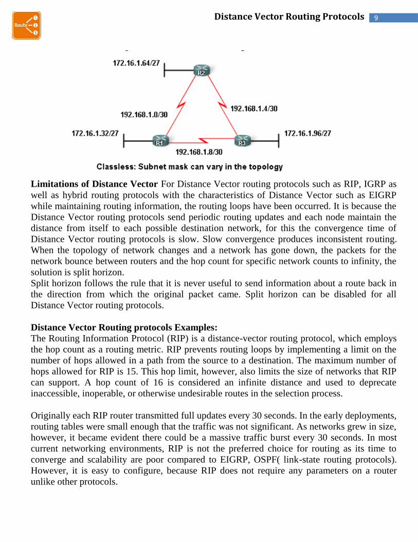
9 Distance Vector Routing Protocols
Limitations of Distance Vector For Distance Vector routing protocols such as RIP, IGRP as
well as hybrid routing protocols with the characteristics of Distance Vector such as EIGRP
while maintaining routing information, the routing loops have been occurred. It is because the
Distance Vector routing protocols send periodic routing updates and each node maintain the
distance from itself to each possible destination network, for this the convergence time of
Distance Vector routing protocols is slow. Slow convergence produces inconsistent routing.
When the topology of network changes and a network has gone down, the packets for the
network bounce between routers and the hop count for specific network counts to infinity, the
solution is split horizon.
Split horizon follows the rule that it is never useful to send information about a route back in
the direction from which the original packet came. Split horizon can be disabled for all
Distance Vector routing protocols.
Distance Vector Routing protocols Examples:
The Routing Information Protocol (RIP) is a distance-vector routing protocol, which employs
the hop count as a routing metric. RIP prevents routing loops by implementing a limit on the
number of hops allowed in a path from the source to a destination. The maximum number of
hops allowed for RIP is 15. This hop limit, however, also limits the size of networks that RIP
can support. A hop count of 16 is considered an infinite distance and used to deprecate
inaccessible, inoperable, or otherwise undesirable routes in the selection process.
Originally each RIP router transmitted full updates every 30 seconds. In the early deployments,
routing tables were small enough that the traffic was not significant. As networks grew in size,
however, it became evident there could be a massive traffic burst every 30 seconds. In most
current networking environments, RIP is not the preferred choice for routing as its time to
converge and scalability are poor compared to EIGRP, OSPF( link-state routing protocols).
However, it is easy to configure, because RIP does not require any parameters on a router
unlike other protocols.

10 Distance Vector Routing Protocols
RIP versions
RIP version 1
The original specification of RIP uses Classful routing. The periodic routing updates do not
carry subnet information, lacking support for variable length subnet masks (VLSM). This
limitation makes it impossible to have different-sized subnets inside of the same network
class. In other words, all subnets in a network class must have the same size.
RIP version 2
Due to the deficiencies of the original RIP specification, RIP version 2 (RIPv2) was
developed. It included the ability to carry subnet information, thus supporting Classless
Inter-Domain Routing (CIDR). To maintain backward compatibility, the hop count limit of
15 remained.
Enabling RIP on a Cisco router RIP can be enabled on a Cisco router by entering router configuration mode from configuration
mode. You must be in exec mode to perform the following commands:
After configuring rip, we can discover routing table by show ip route command:
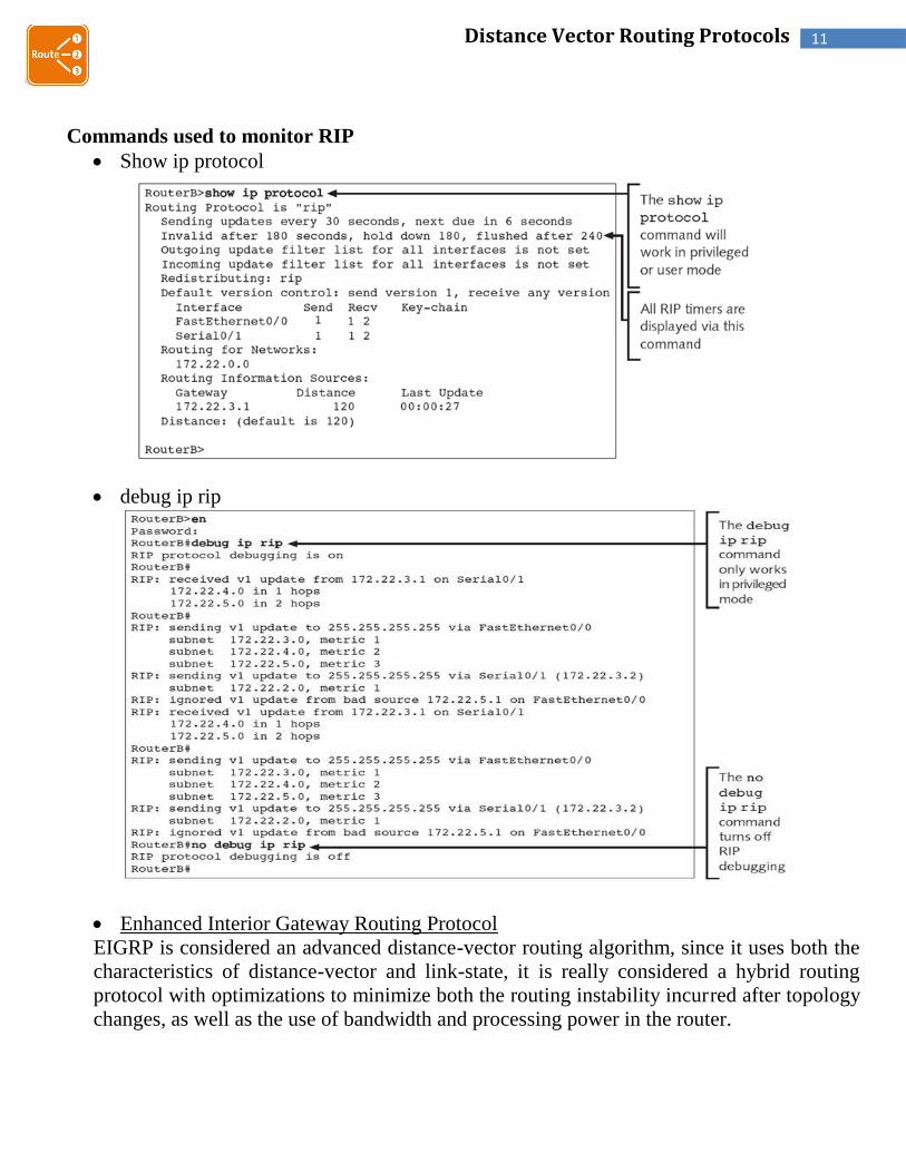
11 Distance Vector Routing Protocols
Commands used to monitor RIP
Show ip protocol
debug ip rip
Enhanced Interior Gateway Routing Protocol
EIGRP is considered an advanced distance-vector routing algorithm, since it uses both the
characteristics of distance-vector and link-state, it is really considered a hybrid routing
protocol with optimizations to minimize both the routing instability incurred after topology
changes, as well as the use of bandwidth and processing power in the router.

12 Distance Vector Routing Protocols
EIGRP stores data in three tables:
Neighbor Table: Stores data about the neighboring routers, i.e. those directly accessible
through directly connected interfaces.
Topology Table: Confusingly named, this table does not store an overview of the
complete network topology; rather, it effectively contains only the aggregation of the
routing tables gathered from all directly connected neighbors. This table contains a list
of destination networks in the EIGRP-routed network together with their respective
metrics.

13 Distance Vector Routing Protocols
Routing table: Stores the actual routes to all destinations
Unlike most other distance vector protocols, EIGRP does not rely on periodic route dumps in
order to maintain its topology table. Routing information is exchanged only upon the
establishment of new neighbor adjacencies, after which only changes are sent.
EIGRP makes use of a composite metric comprised of six different factors:
Hops, Load, Bandwidth, Reliability, Delay, MTU, by default, the formula used for metric
calculation in EIGRP is:
Metric = [(K1*Bandwidth + (K2*Bandwidth)/ (256-load) + K3*Delay)*K5/(reliability +
K4)]*256
EIGRP configuration commands:

14 Distance Vector Routing Protocols
Convergence A dynamic routing protocol must include a set of procedures for a router to inform other
routers about its directly connected networks, to receive and process the same information
from other routers, and to pass along the information it receives from other routers. Further, a
routing protocol must define a metric by which best paths may be determined.
Convergence in RIP Internetworks
RIP for IP, like most distance vector routing protocols, announces its routes in an
unsynchronized and unacknowledged manner. This can lead to convergence problems.
However, you can enable modifications to the announcement algorithms to reduce
convergence time in most situations.
Count-to-Infinity Problem
The classic distance vector convergence problem is known as the count-to-infinity problem and
is a direct result of the asynchronous announcement scheme. When RIP for IP routers add
routes to their routing table, based on routes advertised by other routers, they keep only the
best route in the routing table and they update a lower cost route with a higher cost route only
if is being announced by the same source as the current lower cost route. In certain situations,
as illustrated in the below figures, this causes the count-to-infinity problem.
Assume that the below internetwork has converged. For simplicity, assume that the
announcements sent by Router 1 on Network 1 and Router 2 on Network 3 are not included
Now assume that the link from Router 2 to Network 3 fails and is sensed by Router 2. As
shown in Figure 3.2, Router 2 changes the hop count for the route to Network 3 to indicate that
it is unreachable, an infinite distance away. For RIP for IP, infinity is 16.

15 Distance Vector Routing Protocols
However, before Router 2 can advertise the new hop count to Network 3 in a scheduled
announcement, it receives an announcement from Router 1. The Router 1 announcement
contains a route to Network 3 which is two hops away. Because two hops away is a better route
than 16 hops, Router 2 updates its routing table entry for Network 3, changing it from 16 hops
to three hops, as shown below.
When Router 2 announces its new routes, Router 1 notes that Network 3 is available three hops
away through Router 2. Because the route to Network 3 on Router 1 was originally learned
from Router 2, Router 1 updates its route to Network 3 to four hops.
When Router 1 announces its new routes, Router 2 notes that Network 3 is available four hops
away through Router 1. Because the route to Network 3 on Router 2 was originally learned
from Router 1, Router 2 updates its route to Network 3 to five hops.

16 Distance Vector Routing Protocols
The two routers continue to announce routes to Network 3 with higher and higher hop counts
until infinity (16) is reached. Then, Network 3 is considered unreachable and the route to
Network 3 is eventually timed out of the routing table. This is known as the count-to-infinity
problem.
The count-to-infinity problem is one of the reasons why the maximum hop count of RIP for IP
internetworks is set to 15 (16 for unreachable). Higher maximum hop count values would make
the convergence time longer when count-to-infinity occurs. Also note that during the count-to-
infinity in the previous example, the route from Router 1 to Network 3 is through Router 2.
The route from Router 2 to Network 3 is through Router 1. A routing loop exists between
Router 1 and Router 2 for Network 3 for the duration of the count-to-infinity problem.
Reducing Convergence Time To help reduce the convergence time of RIP for IP internetworks and to avoid count-to-infinity
and routing loops in most situations, you can enable the following modifications to the RIP
announcement mechanism:
Split horizon
Split horizon with poison reverse
Triggered updates
Split Horizon
Split horizon helps reduce convergence time by not allowing routers to advertise networks in
the direction from which those networks were learned. The only information sent in RIP
announcements are for those networks that are beyond the neighboring router in the opposite
direction. Networks learned from the neighboring router are not included.
Split horizon eliminates count-to-infinity and routing loops during convergence in single-path
internetworks and reduces the chances of count-to-infinity in multi-path internetworks. Figure
3.6 illustrates how split horizon keeps the RIP router from advertising routes in the direction
from which they were learned.

17 Distance Vector Routing Protocols
Split Horizon with Poison Reverse
Split horizon with poison reverse differs from simple split horizon because it announces all
networks. However, those networks learned in a given direction are announced with a hop
count of 16, indicating that the network is unreachable. In a single-path internetwork, split
horizon with poison reverse has no benefit beyond split horizon. However, in a multipath
internetwork, split horizon with poison reverse greatly reduces count-to-infinity and routing
loops. Count-to-infinity can still occur in a multipath internetwork because routes to networks
can be learned from multiple sources.
In the below figure, split horizon with poison reverse advertises learned routes as unreachable
in the direction from which they are learned. Split horizon with poison reverse does have the
disadvantage of additional RIP message overhead because all networks are advertised.

18 Distance Vector Routing Protocols
Triggered Updates:
Triggered updates allow a RIP router to announce changes in metric values almost immediately
rather than waiting for the next periodic announcement. The trigger is a change to a metric in
an entry in the routing table. For example, networks that become unavailable can be announced
with a hop count of 16 through a triggered update. Note that the update is sent almost
immediately, where a time interval to wait is typically specified on the router. If triggered
updates were sent by all routers immediately, each triggered update could cause a cascade of
broadcast traffic across the IP internetwork.
Triggered updates improve the convergence time of RIP internetworks but at the expense of
additional broadcast traffic as the triggered updates are propagated.
Distribute a default route with a routing protocol
Let's say you want to use your core router to tell all other routers that they should come
through this core router if they have any network that they can't access. When it comes to
configuring this, each routing protocol is different.
For this example, let's use the Routing Information Protocol (RIP). The best option is to use the
default-information originate command to send a default route to another router. Here's an
example (which assumes we've already configured RIP):
Router(config)# router rip
Router(config-router)# default-information originate
This sends the default route to all other RIP routers.

University of Jordan
Faculty of Engineering & Technology
Computer Engineering Department
Computer Networks Laboratory
907528
Link-State Routing Protocols
2 Link-state routing protocols
Introduction
We can illustrate the difference between link-state and distance vector routing with an analogy.
The analogy stated that distance vector routing protocols are like using road signs to guide you
on your way to a destination, only giving you information about distance and direction.
However, link-state routing protocols are like using a map. With a map, you can see all of the
potential routes and determine your own preferred path.
Distance vector routing protocols are like road signs because routers must make preferred path
decisions based on a distance or metric to a network. Just as travelers trust a road sign to
accurately state the distance to the next town, a distance vector router trusts that another router
is advertising the true distance to the destination network.
Link-state routing protocols take a different approach. Link-state routing protocols are more like
a road map because they create a topological map of the network and each router uses this map
to determine the shortest path to each network. Just as you refer to a map to find the route to
another town, link-state routers use a map to determine the preferred path to reach another
destination.
Routers running link-state routing protocol send information about the state of its links to other
routers in the routing domain. The state of those links refers to its directly connected networks
and includes information about the type of network and any neighboring routers on those
networks-hence the name link-state routing protocol.
The ultimate objective is that every router receives all of the link-state information about all
other routers in the routing area. With this link-state information, each router can create its own
topological map of the network and independently calculate the shortest path to every network.
Link-state routing protocols
Link-state routing protocols are also known as shortest path first protocols and built around
Edsger Dijkstra's shortest path first (SPF) algorithm.
The IP link-state routing protocols are:
Open Shortest Path First (OSPF)
Intermediate System-to-Intermediate System (IS-IS)
Link-state routing protocols have the reputation of being much more complex than their
distance vector counterparts. However, the basic functionality and configuration of link-state
routing protocols is not complex at all. Even the algorithm itself can be easily understood. Basic
OSPF operations can be configured with a router ospfprocess-id command and a network
statement, similar to other routing protocols like RIP and EIGRP.
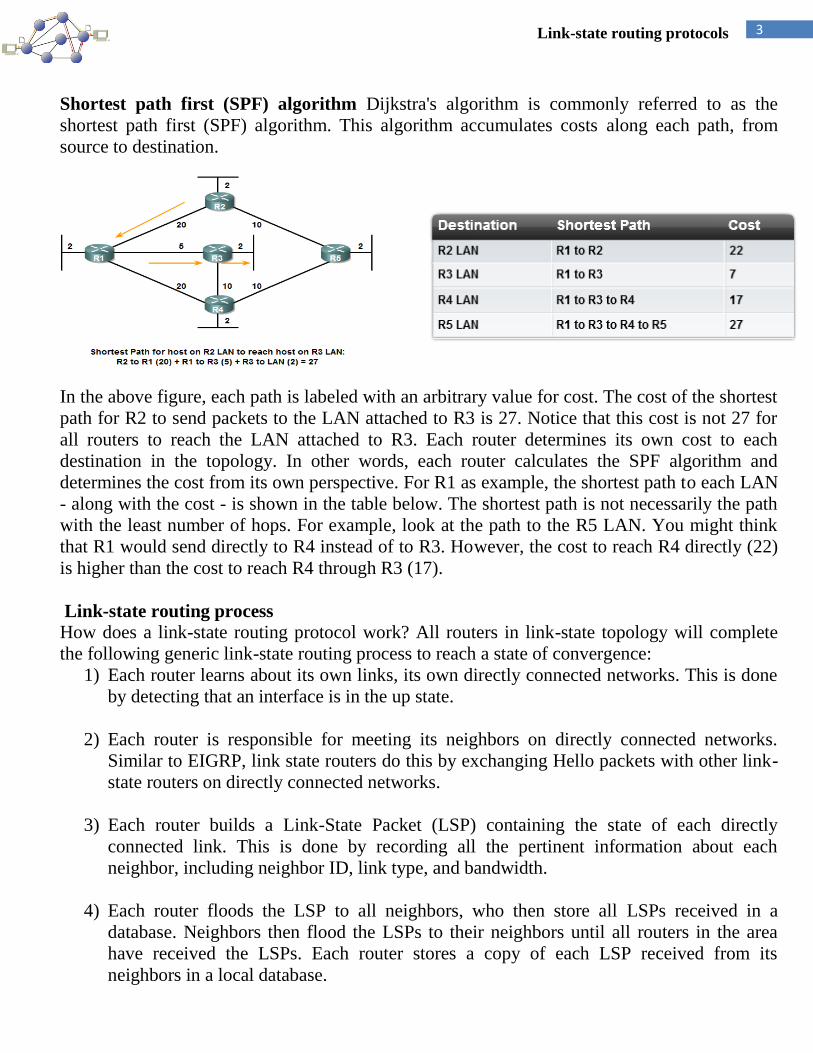
3 Link-state routing protocols
Shortest path first (SPF) algorithm Dijkstra's algorithm is commonly referred to as the
shortest path first (SPF) algorithm. This algorithm accumulates costs along each path, from
source to destination.
In the above figure, each path is labeled with an arbitrary value for cost. The cost of the shortest
path for R2 to send packets to the LAN attached to R3 is 27. Notice that this cost is not 27 for
all routers to reach the LAN attached to R3. Each router determines its own cost to each
destination in the topology. In other words, each router calculates the SPF algorithm and
determines the cost from its own perspective. For R1 as example, the shortest path to each LAN
- along with the cost - is shown in the table below. The shortest path is not necessarily the path
with the least number of hops. For example, look at the path to the R5 LAN. You might think
that R1 would send directly to R4 instead of to R3. However, the cost to reach R4 directly (22)
is higher than the cost to reach R4 through R3 (17).
Link-state routing process
How does a link-state routing protocol work? All routers in link-state topology will complete
the following generic link-state routing process to reach a state of convergence:
1) Each router learns about its own links, its own directly connected networks. This is done
by detecting that an interface is in the up state.
2) Each router is responsible for meeting its neighbors on directly connected networks.
Similar to EIGRP, link state routers do this by exchanging Hello packets with other link-
state routers on directly connected networks.
3) Each router builds a Link-State Packet (LSP) containing the state of each directly
connected link. This is done by recording all the pertinent information about each
neighbor, including neighbor ID, link type, and bandwidth.
4) Each router floods the LSP to all neighbors, who then store all LSPs received in a
database. Neighbors then flood the LSPs to their neighbors until all routers in the area
have received the LSPs. Each router stores a copy of each LSP received from its
neighbors in a local database.

4 Link-state routing protocols
5) Each router uses the database to construct a complete map of the topology and computes
the best path to each destination network. Like having a road map, the router now has a
complete map of all destinations in the topology and the routes to reach them. The SPF
algorithm is used to construct the map of the topology and to determine the best path to
each network.
Advantages of link-state routing protocols
There are several advantages of link-state routing protocols compared to distance vector routing
protocols.
1. Builds a Topological Map
Link-state routing protocols create a topological map, or SPF tree of the network topology.
Distance vector routing protocols do not have a topological map of the network. Routers
implementing a distance vector routing protocol only have a list of networks, which includes
the cost (distance) and next-hop routers (direction) to those networks. Because link-state routing
protocols exchange link-states, the SPF algorithm can build an SPF tree of the network. Using
the SPF tree, each router can independently determine the shortest path to every network.
2. Fast Convergence
When receiving a Link-state Packet (LSP), link-state routing protocols immediately flood the
LSP out all interfaces except for the interface from which the LSP was received. A router using
a distance vector routing protocol needs to process each routing update and update its routing
table before flooding them out other interfaces, even with triggered updates. Faster convergence
is achieved for link-state routing protocols. A notable exception is EIGRP.
3. Event-driven Updates
After the initial flooding of LSPs, link-state routing protocols only send out an LSP when there
is a change in the topology. The LSP contains only the information regarding the affected link.
Unlike some distance vector routing protocols, link-state routing protocols do not send periodic
updates.
4. Hierarchical Design
Link-state routing protocols such as OSPF and IS-IS use the concept of areas. Multiple areas
create a hierarchical design to networks, allowing for better route aggregation (summarization)
and the isolation of routing issues within an area.
Link-state routing protocols requirements
1. Memory Requirements
Link-state routing protocols typically require more memory, more CPU processing, and at times
more bandwidth than distance vector routing protocols. Memory requirements are due to the use
of link-state databases and the creation of the SPF tree.

5 Link-state routing protocols
2. Processing Requirements
Link-state protocols can also require more CPU processing than distance vector routing
protocols. The SPF algorithm requires more CPU time than distance vector algorithms such as
Bellman-Ford because link-state protocols build a complete map of the topology.
3. Bandwidth Requirements
The flooding of link-state packets can adversely affect the available bandwidth on a network.
This should only occur during initial startup of routers, but can also be an issue on unstable
networks.
Open Shortest Path First (OSPF)
OSPF is a link-state routing protocol that was developed as a replacement for the distance
vector routing protocol RIP. RIP was an acceptable routing protocol in the early days of
networking and the Internet, but its reliance on hop count as the only measure for choosing the
best route quickly became unacceptable in larger networks that needed a more robust routing
solution. OSPF is a classless routing protocol that uses the concept of areas for scalability. RFC
2328 defines the OSPF metric as an arbitrary value called cost. The Cisco IOS uses bandwidth
as the OSPF cost metric. OSPF's major advantages over RIP are its fast convergence and its
scalability to much larger network implementations.
OSPF message encapsulation
The data portion of an OSPF message is encapsulated in a packet. This data field can include
one of five OSPF packet types The OSPF packet header is included with every OSPF packet,
regardless of its type. The OSPF packet header and packet type-specific data are then
encapsulated in an IP packet.
1) Hello - Hello packets are used to establish and maintain adjacency with other
OSPF routers.
2) DBD - The Database Description (DBD) packet contains an abbreviated list of the
sending router's link-state database and is used by receiving routers to check
against the local link-state database.
3) LSR - Receiving routers can then request more information about any entry in the
DBD by sending a Link-State Request (LSR).
4) LSU - Link-State Update (LSU) packets are used to reply to LSRs as well as to
announce new information. LSUs contain seven different types of Link-State
Advertisements (LSAs).
5) LSAck - When an LSU is received, the router sends a Link-State
Acknowledgement (LSAck) to confirm receipt of the LSU.

6 Link-state routing protocols
The basic OSPF configuration
The router ospf command OSPF is enabled with the router ospf process-id global configuration command. The process-id
is a number between 1 and 65535 and is chosen by the network administrator. The process-id is
locally significant, which means that it does not have to match other OSPF routers in order to
establish adjacencies with those neighbors. In our topology we will enable OSPF on all three
routers using the same process ID of 1. We are using the same process ID simply for
consistency.
R1(config)#router ospf 1
R2(config)#router ospf 1
R3(config)#router ospf 1
The network command The network command used with OSPF has the same function as
when used with other IGP routing protocols: Any interfaces on a router that match the network
address in the network command will be enabled to send and receive OSPF packets. This
network (or subnet) will be included in OSPF routing updates. The network command is used in
router configuration mode.
Router(config-router)#network network-address wildcard-mask area area-id
The OSPF network command uses a combination of network-address and wildcard-mask. The
network address along with the wildcard mask is used to specify the interface or range of
interfaces that will be enabled for OSPF using this network command. The wildcard mask can
be configured as the inverse of a subnet mask. For example, R1's FastEthernet 0/0 interface is
on the 172.16.1.16/28 network. The subnet mask for this interface is /28 or 255.255.255.240.
The inverse of the subnet mask results in the wildcard mask.
255.255.255.255
- 255.255.255.252 Subtract the subnet mask
---------------
0. 0. 0. 3 Wildcard mask

7 Link-state routing protocols
The area area-id refers to the OSPF area. An OSPF area is a group of routers that share link-
state information. All OSPF routers in the same area must have the same link-state information
in their link-state databases. This is accomplished by routers flooding their individual link-states
to all other routers in the area.
When all of the routers are within the same OSPF area, the network commands must be
configured with the same area-id on all routers. Although any area-id can be used, it is good
practice to use an area-id of 0 with single-area OSPF. This convention makes it easier if the
network is later configured as multiple OSPF areas where area 0 becomes the backbone area.
The configuration below shows the network commands for all three routers, enabling OSPF on
all interfaces. At this point all routers should be able to ping all networks.
Verifying OSPF
Some powerful OSPF troubleshooting commands include:
#show ip ospf neighbor
#show ip protocols
#show ip ospf
#show ip ospf interface
The show ip ospf neighbor command can be used to verify and troubleshoot OSPF neighbor
relationships. For each neighbor, this command displays the following output:
Neighbor ID - The router ID of the neighboring router.
Pri - The OSPF priority of the interface.
State - The OSPF state of the interface. FULL state means that the router and its
neighbor have identical OSPF link-state databases.
Dead Time - The amount of time remaining that the router will wait to receive an
OSPF Hello packet from the neighbor before declaring the neighbor down. This value
is reset when the interface receives a Hello packet.

8 Link-state routing protocols
Address - The IP address of the neighbor's interface to which this router is directly
connected.
Interface - The interface on which this router has formed adjacency with the neighbor.
The show ip protocols command is a quick way to verify vital OSPF configuration information,
including the OSPF process ID, the router ID, networks the router is advertising, the neighbors
the router is receiving updates from, and the default administrative distance, which is 110 for
OSPF.
The show ip ospf command can also be used to examine the OSPF process ID and router ID.
Additionally, this command displays the OSPF area information as well as the last time the SPF
algorithm was calculated. As you can see from the sample output, OSPF is a very stable routing
protocol. The only OSPF-related event that R1 has participated in during the past 11 and half
hours is to send small Hello packets to its neighbors.
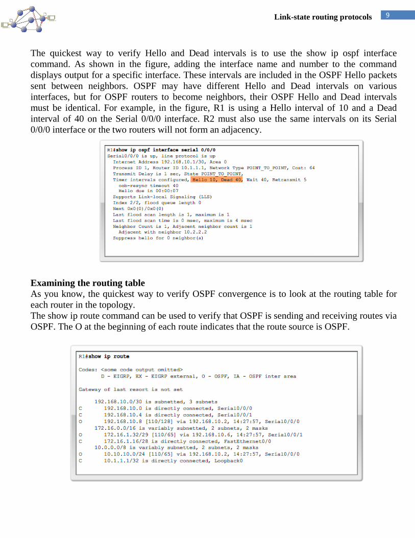
9 Link-state routing protocols
The quickest way to verify Hello and Dead intervals is to use the show ip ospf interface
command. As shown in the figure, adding the interface name and number to the command
displays output for a specific interface. These intervals are included in the OSPF Hello packets
sent between neighbors. OSPF may have different Hello and Dead intervals on various
interfaces, but for OSPF routers to become neighbors, their OSPF Hello and Dead intervals
must be identical. For example, in the figure, R1 is using a Hello interval of 10 and a Dead
interval of 40 on the Serial 0/0/0 interface. R2 must also use the same intervals on its Serial
0/0/0 interface or the two routers will not form an adjacency.
Examining the routing table
As you know, the quickest way to verify OSPF convergence is to look at the routing table for
each router in the topology.
The show ip route command can be used to verify that OSPF is sending and receiving routes via
OSPF. The O at the beginning of each route indicates that the route source is OSPF.


![ANNA UNIVERSITY COIMBATORE [Regulation 2008] B E ...enggedu.com/tamilnadu/university_syllabus/cse_5_8sem.pdfObject Oriented Systems Lab 0 0 3 2 Computer Graphics Lab 0 0 3 2 . Semester](https://static.fdocuments.us/doc/165x107/5f0e3e837e708231d43e4dda/anna-university-coimbatore-regulation-2008-b-e-object-oriented-systems-lab.jpg)