L6-9 Chapter 2
43
Process Dynamics and Control CCB3013 - Chemical Process Dynamics, Instrumentation and Control 1 6/10/2014 Chapter 2 Mathematical Modeling of Chemical Processes
-
Upload
syed-nazrin -
Category
Documents
-
view
3 -
download
0
description
good
Transcript of L6-9 Chapter 2

Pro
cess D
yn
am
ics a
nd
Co
ntr
ol
CCB3013 - Chemical Process Dynamics, Instrumentation
and Control 16/10/2014
Chapter 2
Mathematical Modeling of
Chemical Processes
Pro
cess D
yn
am
ics a
nd
Co
ntr
ol
CCB3013 - Chemical Process Dynamics, Instrumentation
and Control 26/10/2014
Chapter Objectives
End of this chapter, you should be able to:
1. Develop unsteady-state models (dynamic models) of
chemical processes from physical and chemical principles
2. Explain the rationale for dynamic models
3. Explain a general strategy for deriving dynamic models
4. Carry out simulation studies (Solution of the dynamic
models that consist of sets of ODE’s and AE’s)

Pro
cess D
yn
am
ics a
nd
Co
ntr
ol
CCB3013 - Chemical Process Dynamics, Instrumentation
and Control 36/10/2014
Mathematical Model (Eykhoff, 1974)
• “a representation of the essential aspects of an
existing system (or a system to be constructed)
which represents knowledge of that system in a
usable form”
• Everything should be made as simple as possible,
but no simpler

Pro
cess D
yn
am
ics a
nd
Co
ntr
ol
CCB3013 - Chemical Process Dynamics, Instrumentation
and Control 46/10/2014
Uses of mathematical models
Design:
• Exploring the sizing and arrangement of processing
equipment for dynamic performance
• Studying the interactions of various parts of the
process, particularly when material recycle or heat
integration is used
• Evaluating alternate process and control structures
and strategies
• Simulating start-up, shutdown, and emergency
simulations and procedures.

Pro
cess D
yn
am
ics a
nd
Co
ntr
ol
CCB3013 - Chemical Process Dynamics, Instrumentation
and Control 56/10/2014
Uses of mathematical models
Plant operation:
• Troubleshooting and processing problems
• Aiding in start-up and operator training
• Studying the effects of and the requirements for
expansion (bottle-neck removal) projects
• Optimizing plant operation
• It is usually much cheaper, safer, and faster to
conduct the kinds of studies listed above on a
mathematical model than experimentally on an
operating unit.

Pro
cess D
yn
am
ics a
nd
Co
ntr
ol
CCB3013 - Chemical Process Dynamics, Instrumentation
and Control 66/10/2014
Principles of Model Formulation
• The model equations are at best an
approximation to the real process.
• Adage: “All models are wrong, but some are
useful”
• Inherently involves a compromise between
– model accuracy and complexity
– the and effort required to develop the
model

Pro
cess D
yn
am
ics a
nd
Co
ntr
ol
CCB3013 - Chemical Process Dynamics, Instrumentation
and Control 76/10/2014
Process modeling
• Both an art and a science.
• Requires creativity to make simplifying
assumptions that result in an appropriate
model
• Dynamic models of chemical processes
consist of ODEs and/or PDEs, plus related
algebraic equations
Pro
cess D
yn
am
ics a
nd
Co
ntr
ol
CCB3013 - Chemical Process Dynamics, Instrumentation
and Control 86/10/2014
A Systematic Approach for Developing
Dynamic Models
1. State the modeling objectives and the end use of
the model. They determine the required levels of
model detail and model accuracy.
2. Draw a schematic diagram of the process and label
all process variables.
3. List all of the assumptions that are involved in
developing the model. Try for parsimony; the
model should be no more complicated than
necessary to meet the modeling objectives.

Pro
cess D
yn
am
ics a
nd
Co
ntr
ol
CCB3013 - Chemical Process Dynamics, Instrumentation
and Control 96/10/2014
Systematic Approach
4. Determine whether spatial variations of process
variables are important. If so, a partial differential
equation model will be required.
5. Write appropriate conservation equations (mass,
component, energy, and so forth).
6. Introduce equilibrium relations and other algebraic
equations (from thermodynamics, transport
phenomena, chemical kinetics, equipment
geometry, etc.).

Pro
cess D
yn
am
ics a
nd
Co
ntr
ol
CCB3013 - Chemical Process Dynamics, Instrumentation
and Control 106/10/2014
A Systematic Approach…
6. Perform a degrees of freedom analysis (Section 2.3) to ensure that the model equations can be solved.
7. Simplify the model.
• Arrange the equations so that the dependent variables (outputs) appear on the left side and the independent variables (inputs) appear on the right side.
• This model form is convenient for computer simulation and subsequent analysis.
8. Classify inputs as disturbance variables or as manipulated variables.
Pro
cess D
yn
am
ics a
nd
Co
ntr
ol
CCB3013 - Chemical Process Dynamics, Instrumentation
and Control 116/10/2014
Modeling Approaches
Physical/chemical (fundamental, global)
• Model structure by theoretical analysis
– Material/energy balances
– Heat, mass, and momentum transfer
– Thermodynamics, chemical kinetics
– Physical property relationships
• Model complexity must be determined (assumptions)
• Can be computationally expensive (not real-time)
• May be expensive/time-consuming to obtain
• Good for extrapolation, scale-up
• Does not require experimental data to obtain (data
required for validation and fitting)
• Theoretical models of chemical processes are based on
conservation laws.

Pro
cess D
yn
am
ics a
nd
Co
ntr
ol
CCB3013 - Chemical Process Dynamics, Instrumentation
and Control 126/10/2014
Mass Balance
Conservation of Component i
rate of mass rate of mass rate of mass(2-6)
accumulation in out
(2.1)
rate of component i rate of component i
accumulation in
rate of component i rate of component i(2-7)
out produced
(2.2)
Conservation of Mass

Pro
cess D
yn
am
ics a
nd
Co
ntr
ol
CCB3013 - Chemical Process Dynamics, Instrumentation
and Control 136/10/2014
Energy Balance
Conservation of Energy
rate of energy rate of energy in rate of energy out
accumulation by convection by convection
net rate of heat addition net rate of work
to the system from performed on the sys
the surroundings
tem (2-8)
by the surroundings (2.3)

Pro
cess D
yn
am
ics a
nd
Co
ntr
ol
CCB3013 - Chemical Process Dynamics, Instrumentation
and Control 146/10/2014
Energy Balance …
• Total energy of a system, Utot
int (2-9)tot KE PEU U U U (2.4)
• For the processes and examples considered in
this course, it is appropriate to make two
assumptions:
– Changes in potential energy and kinetic
energy can be neglected
– The net rate of work can be neglected

Pro
cess D
yn
am
ics a
nd
Co
ntr
ol
CCB3013 - Chemical Process Dynamics, Instrumentation
and Control 156/10/2014
Energy Balance …
• For these reasonable assumptions, the energy balance in Eq.
2-3 can be written as
int the internal energy of
the system
enthalpy per unit mass
mass flow rate
rate of heat transfer to the system
U
H
w
Q
denotes the difference
between outlet and inlet
conditions of the flowing
streams; therefore
-Δ wH = rate of enthalpy of the inlet
stream(s) - the enthalpy
of the outlet stream(s)
int (2-10)dU
wH Qdt
(2.5)

Pro
cess D
yn
am
ics a
nd
Co
ntr
ol
CCB3013 - Chemical Process Dynamics, Instrumentation
and Control 166/10/2014
Black box (empirical)
– Large number of unknown parameters
– Can be obtained quickly (e.g., linear
regression)
– Model structure is subjective
– Dangerous to extrapolate

Pro
cess D
yn
am
ics a
nd
Co
ntr
ol
CCB3013 - Chemical Process Dynamics, Instrumentation
and Control 176/10/2014
• Compromise of first two approaches
• Model structure may be simpler
• Typically 2 to 10 physical parameters estimated
(nonlinear regression)
• Good versatility, can be extrapolated
• Can be run in real-time
• linear regression
• nonlinear regression
Semi-empirical
2
210 xcxccy
/1 teKy
Pro
cess D
yn
am
ics a
nd
Co
ntr
ol
CCB3013 - Chemical Process Dynamics, Instrumentation
and Control 186/10/2014
Semi-empirical
• Number of parameters affects accuracy of model,
but confidence limits on the parameters fitted must
be evaluated.
• Objective function for data fitting – minimize sum of
squares of errors between data points and model
predictions (use optimization code to fit parameters)
• Nonlinear models such as neural nets are becoming
popular (automatic modeling)
Pro
cess D
yn
am
ics a
nd
Co
ntr
ol
CCB3013 - Chemical Process Dynamics, Instrumentation
and Control 196/10/2014
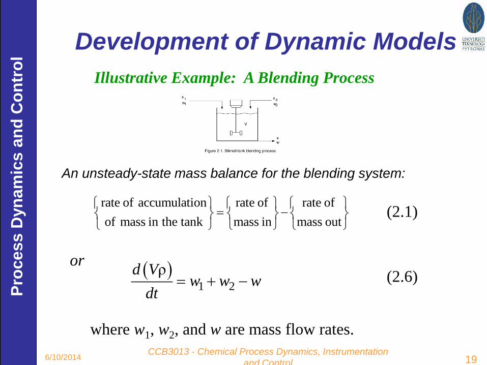
Development of Dynamic Models
An unsteady-state mass balance for the blending system:
rate of accumulation rate of rate of(2-1)
of mass in the tank mass in mass out
1 2
ρ(2-2)
d Vw w w
dt
(2.1)
(2.6)
where w1, w2, and w are mass flow rates.
or
Illustrative Example: A Blending Process

Pro
cess D
yn
am
ics a
nd
Co
ntr
ol
CCB3013 - Chemical Process Dynamics, Instrumentation
and Control 206/10/2014
Blending Process
The corresponding steady-state model was derived in
Ch. 1 (cf. Eqs. 1-1 and 1-2).
1 2
1 1 2 2
0 (2-4)
0 (2-5)
w w w
w x w x wx
(2.8)
(2.7)
1 1 2 2
ρ(2-3)
d V xw x w x wx
dt
The unsteady-state component balance is:

Pro
cess D
yn
am
ics a
nd
Co
ntr
ol
CCB3013 - Chemical Process Dynamics, Instrumentation
and Control 216/10/2014
Equation 2-10 can be simplified by expanding the
accumulation term using the “chain rule” for
differentiation of a product:
The Blending Process Revisited
1 2 (2-12)dV
w w wdt
(2.9)
1 1 2 2 (2-13)
d Vxw x w x wx
dt
(2.10)
For constant ρ, Eqs. 2-6 and 2-7 become:
Substitution of (2-11) into (2-10) gives:
(2.12)1 1 2 2 (2-15)
dx dVV x w x w x wx
dt dt
(2.11) (2-14)
d Vx dx dVV x
dt dt dt

Pro
cess D
yn
am
ics a
nd
Co
ntr
ol
CCB3013 - Chemical Process Dynamics, Instrumentation
and Control 226/10/2014
Blending Process Revisited …
Substitution of the mass balance in (2-9) for in (2-12) gives:
(2.13) 1 2 1 1 2 2 (2-16)dx
V x w w w w x w x wxdt
After canceling common terms and rearranging (2-9) and
(2-13), a more convenient model form is obtained:
(2.14)
(2.15)
1 2
1 21 2
1(2-17)
(2-18)
dVw w w
dt
w wdxx x x x
dt V V

Pro
cess D
yn
am
ics a
nd
Co
ntr
ol
CCB3013 - Chemical Process Dynamics, Instrumentation
and Control 236/10/2014
Blending Process Revisited …
• The dynamic model in Eqs. 2-14 and 2-15 is in a
convenient form for subsequent investigation based on
analytical or numerical techniques
• Specify the inlet compositions (x1 and x2) and the flow
rates (w1, w2 and w) as functions of time
• Specify the initial conditions for the dependent variables,
V(0) and x(0)
• Determine the transient responses, V(t) and x(t)

Pro
cess D
yn
am
ics a
nd
Co
ntr
ol
CCB3013 - Chemical Process Dynamics, Instrumentation
and Control 246/10/2014
Blending Process Revisited …

Pro
cess D
yn
am
ics a
nd
Co
ntr
ol
CCB3013 - Chemical Process Dynamics, Instrumentation
and Control 256/10/2014
Dynamic models of representative
processes
• Stirred-Tank Heating Process
Figure 2.3 Stirred-tank heating process with constant holdup, V.
Pro
cess D
yn
am
ics a
nd
Co
ntr
ol
CCB3013 - Chemical Process Dynamics, Instrumentation
and Control 266/10/2014
Assumptions:
• Perfect mixing
The exit temperature T is also the temperature of
the tank contents
• The liquid holdup V is constant because the inlet and
outlet flow rates are equal
• The density ρ and heat capacity C of the liquid are
assumed to be constant
Temperature dependence is neglected
• Heat losses are negligible
Stirred-Tank Heating Process

Pro
cess D
yn
am
ics a
nd
Co
ntr
ol
CCB3013 - Chemical Process Dynamics, Instrumentation
and Control 276/10/2014
Stirred-Tank Heating Process
intˆ ˆ (2-29)dU dH CdT (2.16)
Model Development
• For a pure liquid at low or moderate pressures, the internal
energy, Uint, is approximately equal to the enthalpy, H
• H depends only on temperature
• We assume that Uint = H and where the caret (^) means per
unit mass.
A differential change in temperature, dT, produces a
corresponding change in the internal energy per unit mass,
where C is the constant pressure heat capacity.
(2.17)int intˆ (2-30)U VU
The total internal energy of the liquid in the tank is:

Pro
cess D
yn
am
ics a
nd
Co
ntr
ol
CCB3013 - Chemical Process Dynamics, Instrumentation
and Control 286/10/2014
Stirred-Tank Heating Process
An expression for the rate of internal energy accumulation
can be derived from Eqs. (2-16) and (2-17):
(2.18)int (2-31)dU dT
VCdt dt
• Note that this term appears in the general energy
balance of Eq. 2-5.
(2.19) ˆ ˆ (2-32)ref refH H C T T
Suppose that the liquid in the tank is at a temperature T
and has an enthalpy, . Integrating Eq. 2-16 from a
reference temperature Tref to T gives,
H

Pro
cess D
yn
am
ics a
nd
Co
ntr
ol
CCB3013 - Chemical Process Dynamics, Instrumentation
and Control 296/10/2014
Stirred-Tank Heating Process
Without loss of generality, we assume that .
Thus, (2-19) can be written as:
0ˆ refH
(2.20) ˆ (2-33)refH C T T
(2.21)For the inlet stream: ˆ (2-34)i i refH C T T
Substituting (2-20) and (2-21) into the convection term
of (2-5) gives:
(2.22) ˆ (2-35)i ref refwH w C T T w C T T
Finally, substitution of (2-18) and (2-22) into (2-5)
(2.23) (2-36)i
dTV C wC T T Q
dt
Pro
cess D
yn
am
ics a
nd
Co
ntr
ol
CCB3013 - Chemical Process Dynamics, Instrumentation
and Control 306/10/2014
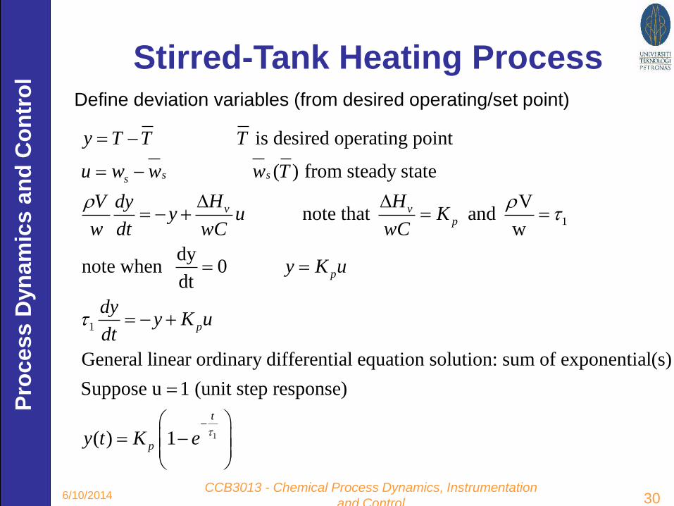
Stirred-Tank Heating Process
1
1
is desired operating point
( ) from steady state
Vnote that and
w
dynote when 0
dt
General linear ordinary differential equation solution:
s ss
v vp
p
p
y T T T
u w w w T
H HV dyy u K
w dt wC wC
y K u
dyy K u
dt
1
sum of exponential(s)
Suppose u 1 (unit step response)
( ) 1
t
py t K e
Define deviation variables (from desired operating/set point)

Pro
cess D
yn
am
ics a
nd
Co
ntr
ol
CCB3013 - Chemical Process Dynamics, Instrumentation
and Control 316/10/2014
Stirred-Tank Heating Process

Pro
cess D
yn
am
ics a
nd
Co
ntr
ol
CCB3013 - Chemical Process Dynamics, Instrumentation
and Control 326/10/2014
Example 1:
6
s
v
o
4
3 3
3
4
w =0.83 10 g hr
H =600 cal g
C=l cal g C
w=10 kg hr
=10 kg m
V=20 m
2 10 kgV
4
4
V 2 10 kg2hr
w 10 kg hr
C0= C,90= C,40= o
i
oo
i TTT
The dynamic model is
u106+-y=dt
dy2 5-
ss wwu
TTy
Steady-state balance:
vsi ΔHw)=-TTwC(
hr/kg) ( 106
) (cal/g 1 (g/hr) 1010
)cal/g(600
o5
o34
C
CwC
HK v
p

Pro
cess D
yn
am
ics a
nd
Co
ntr
ol
CCB3013 - Chemical Process Dynamics, Instrumentation
and Control 336/10/2014
Example 1:
0=y(0) T=T(0)
Step 1: at t=0 double ws
hrg10+0.83=u 6
50+-y=dt
dy2
C140=90+50=T+y=T o
ssFinal
-0.5te-l50=y
t = 0
ws
sw
50
1083.0106 65
uK p

Pro
cess D
yn
am
ics a
nd
Co
ntr
ol
CCB3013 - Chemical Process Dynamics, Instrumentation
and Control 346/10/2014
Example 1:
hr 24 / C140 = oTStep 2: Maintain New steady
state
Step 3: Then set hrkg830 = 0, = swu
50=(0) ,106+-=2 5- yuydt
dy
Solve for u = 0
0 , as
50= -0.5
yt
ey t
How long to reach y = 0.5 ?
Self-regulating, but slow

Pro
cess D
yn
am
ics a
nd
Co
ntr
ol
CCB3013 - Chemical Process Dynamics, Instrumentation
and Control 356/10/2014
Example 1:
Step 4: How can we speed up the return from 140°C to
90°C?
Now, find the time to reach y = 0.5?
ws = 0 g/hr u = -0.83 x 10⁶ g/hr
50--=2 ydt
dy tey -0.5-l50- =
At steady state with ws =0, y -50°C T 40°C
Definitely much quicker
than the case u = 0

Pro
cess D
yn
am
ics a
nd
Co
ntr
ol
CCB3013 - Chemical Process Dynamics, Instrumentation
and Control 366/10/2014
Process Dynamics• Process control is inherently concerned with unsteady
state behavior, i.e., "transient response", "process
dynamics"
Stirred tank heater: Assume a "lag" between heating element
temperature Te, and process fluid temp, T.
Heat transfer limitation = he A(Te – T)
Energy balances
Tank:
Heating element:dt
dTC-T)=mA(TQ-h e
eeee
0 0, dt
dT
dt
dT eAt steady state :
dt
dTmCwCTTTAhwCT eei )(

Pro
cess D
yn
am
ics a
nd
Co
ntr
ol
CCB3013 - Chemical Process Dynamics, Instrumentation
and Control 376/10/2014
Process Dynamics
Specify Q Calculate T, Te
2 first order equations 1 second order equation in T
Relate T to Q (Te is an intermediate variable)
fixed i TQ- u=QTy=T-
Note Ce 0 yields 1st order ODE (simpler model)
uwC
ydt
dy
w
m
wC
Cm
Ah
Cm
dt
yd
Ah
Cmm ee
ee
ee
ee
ee 1 2
2

Pro
cess D
yn
am
ics a
nd
Co
ntr
ol
CCB3013 - Chemical Process Dynamics, Instrumentation
and Control 386/10/2014
Liquid storage systems
h R
1=q
v
Rv: line resistance
57)-(2 1
hR
qdt
dhA
v
i
linear ODE
pressureambient : aav P P-Pq=C
ghpP If
* (2-61)i v i v
dhA q C ρgh q C h
dt
Non-linear
ODE

Pro
cess D
yn
am
ics a
nd
Co
ntr
ol
CCB3013 - Chemical Process Dynamics, Instrumentation
and Control 396/10/2014
Degrees of Freedom Analysis
1. List all quantities in the model that are known constants
(or parameters that can be specified) on the basis of
equipment dimensions, known physical properties, etc.
2. Determine the number of equations NE and the number
of process variables, NV. Note that time t is not
considered to be a process variable because it is neither
a process input nor a process output.
3. Calculate the number of degrees of freedom, NF = NV -
NE.

Pro
cess D
yn
am
ics a
nd
Co
ntr
ol
CCB3013 - Chemical Process Dynamics, Instrumentation
and Control 406/10/2014
Degrees of Freedom
4. Identify the NE output variables that will be obtained
by solving the process model.
5. Identify the NF input variables that must be specified as
either disturbance variables or manipulated variables, in
order to utilize the NF degrees of freedom.

Pro
cess D
yn
am
ics a
nd
Co
ntr
ol
CCB3013 - Chemical Process Dynamics, Instrumentation
and Control 416/10/2014
Degrees of Freedom Analysis
for the Stirred-Tank Model
, ,V CParameters (3): , , ,iT T w QVariables (4):
Equation (1) : Eq. 2-23 NF = 4 – 1 = 3
The process variables are classified as:
Output variable: T Input variables : Ti, w, Q
For temperature control purposes, it is reasonable to classify
the three inputs as:
Disturbance variables : Ti, w
Manipulated variable : Q
Pro
cess D
yn
am
ics a
nd
Co
ntr
ol
CCB3013 - Chemical Process Dynamics, Instrumentation
and Control 426/10/2014
Conclusion!
• Need for mathematical modeling
• Types of mathematical models
• A systematic approach
• Blending example – revisited
• Tank heater example – model developed
• Second-order system
• Linear and nonlinear systems
• Degrees of freedom

Pro
cess D
yn
am
ics a
nd
Co
ntr
ol
CCB3013 - Chemical Process Dynamics, Instrumentation
and Control 436/10/2014
For Chapter 3
• Go through Laplace Transform
• Xerox Laplace Transform Table 3.1
page 54-55, Seborg Book