Il L J

n . I I ...

r-l ) r

: J

[J. ~---j

\,.)

)] rJ) L

! I r

,--,

i I

UNIVERSITY OF MINNESOTA ST. ANTHONY FALLS LABORATORY

Engineering, Environmental and Geophysical Fluid Dynamics

Project Report No. 402

Numerical Simulation of Cavitating and Non~cavitating Flows over a Hydrofoil

by

Charles C.S. Song,

Jianming He, Fayi Zhou,. and Ge Wang

Prepared for

Office of Naval Research U. S. Navy, Department of Defense

Under Contract No. N/N00014~96~1-0128

April 1997 Minneapolis, Minnesota

The University of Minnesota is committed to the policy that all persons shall have equal access to its programs, facilities, and employment without regard to race, religion, color, sex, national origin, handicap, age or veteran status.

LastRevised: Aprll28,1997 Disk Locators: MSWord\ Winword\docs\PR4020NR.doc

PR403c.ov.doc (a:\\Disk #211)

ii

,._, I : I I

I I

r i I i

I!

I 1 LJ

! I i

TABLE OF CONTENTS

Acknowledgements ......... ,., .. , ... " .. , ... , .. " ........ , ............. , ................... ,""', ... iv Abstract ..... " ... ,., ....................... " ..... , ...... , ... , ........ ,"', ................. " ...... v List of Figures .................................. ,',.,." ... ,""""',. "., " .... , .... , ........... , ... ". vi

I. Introduction ",.,', ................................................. , ..... ,', .......... ,"' ... " ....... ,. 1

II. Theoretical Considerations, .. , .. ,", .. , ... ,.,.,', ...... " ...... , .... ,', .. "., .. , ..... , ... , ... , .. ,. 3

III. Numerical Approach" ....... " .... ", .... , .... ,.,.,',., ............................................. 5

IV. Non-Cavitating Flow Over A FoiL ............................................................. 7 4-1 Previous Studies ................................................................................. 7 4-2 Model Validation ............................................................................... 8 4-3 Unsteady Structures ........................................................................... 9

4.3 .1 Trailing edge unsteadiness (a=6°) ........................................... 9 4.3.2 Leading edge separation (a= 10°) ............................................ 9 4.3.3 Large vortex washout (a=15°) ................................................ 10 4.3.4 High attack angle stall (a=200) ............................................... 11

V. Cavitating Flow Over A Thin Foi1. ............ , ............................................... , 12. 5.1 Non-Cavitating Flow Results .............................................................. 12 5.2 Cavitating Flow Results ......................................... , ............................ 13

VI. Cavitating Flow Over a Thin Foi1. .............................................................. 16 6.1 Comparison with Experiments ............................................................ 16 6.2 Qualitative Description of Two-Dimensional Cavity Flows ................. 17

6.2.1 Moving and fixed (sheet) cavitation at small attack angle ........ 17 6.2.2 Intermittent occurrence of cloud cavitation at

medium attack angle .............................................................. 17 6.2.3 Continuous occurrence of cloud cavitation at

large attack angle ........................................... , .......... , ........... 18 6.3 Three Dimensionality of Cavitating Flow

VII. Conclusions .............................................................................................. 19

References ............................................................................................. 21

Figures 4-1 through 6-23

iii

ACKNOWLEDGMENTS

This study is sponsored by the Office of Naval Research under Contract No. NINO 00 14-96-0128. Dr. X. Y. Chen provided some help at the early stage of the program setup. The computer time has been provided by the Minnesota Supercomputer Institute, University of Minnesota through its grant program.

iv

fi

1

I-I I

'1 I I

U

[j

U fl Lj

[1 Ll

1 J

ABSTRACT

The compressible hydrodynamic approach previously developed for small Mach number non~cavitating flows has been extended to simulate cavitating flows as well as non~cavitatingflows. The extension is made possible by assuming a complex equation of state relating density and pressure to cover the liquid phase and the gas phase. Thus, the cavitation phenomenon is regarded as a single~phase flow phenomenon enabling the elimination of the cavity closure condition. The numerical model is an unsteady 3~ dimensional flow model based on a large eddy simulation approach. It is applied to typical thin hydrofoils and thick hydrofoils at non~cavitating conditions and various cavitating flow conditions, including moving cavity, stable sheet cavity and sheet cavity/cloud cavity cyclical flow conditions. Computations are carried out primarily for 2~dimensional foils, but 3~dimensional flow characteristics are also examined.

The computational results are compared with some available data;. good quantitative and qualitative agreements are indicated. It is considered very significant that the sheet cavitation/cloud cavitation phenomenon is found to be similar to the viscous boundary layer flow separation/vortex shedding and washout phenomenon in many respects. Cavitation is found to trigger boundary layer separation in otherwise non~ separated flow. -

v

Fig. 4-1

Fig. 4-2

Fig. 4-3

Fig. 4-4

Fig. 4-5

Fig. 4-6 .

Fig. 4-7

Fig. 4-8

Fig. 4-9

Fig. 4-10

Fig. 4-11

Fig. 4-12

Fig. 4-13

Fig. 5-1

LIST OF FIGURES

Medium mesh system (381x64x3) around a NACA0015 foil.

Comparison of computed pressure coefficients with experiment data (Izumida et aI., 1980) for NACA0015 foil at non-cavitating condition.

Computed pressure coefficient distributions along foil surface based on three different mesh systems: coarse mesh (191x32x3), medium mesh (381x64x3), and fine mesh (761xI28x3).

Instantaneous vorticity component (ooz) contours on the mid-span cross­section of NACA662-415 foil at 0.=6° during one period of trailing edge vortex shedding .

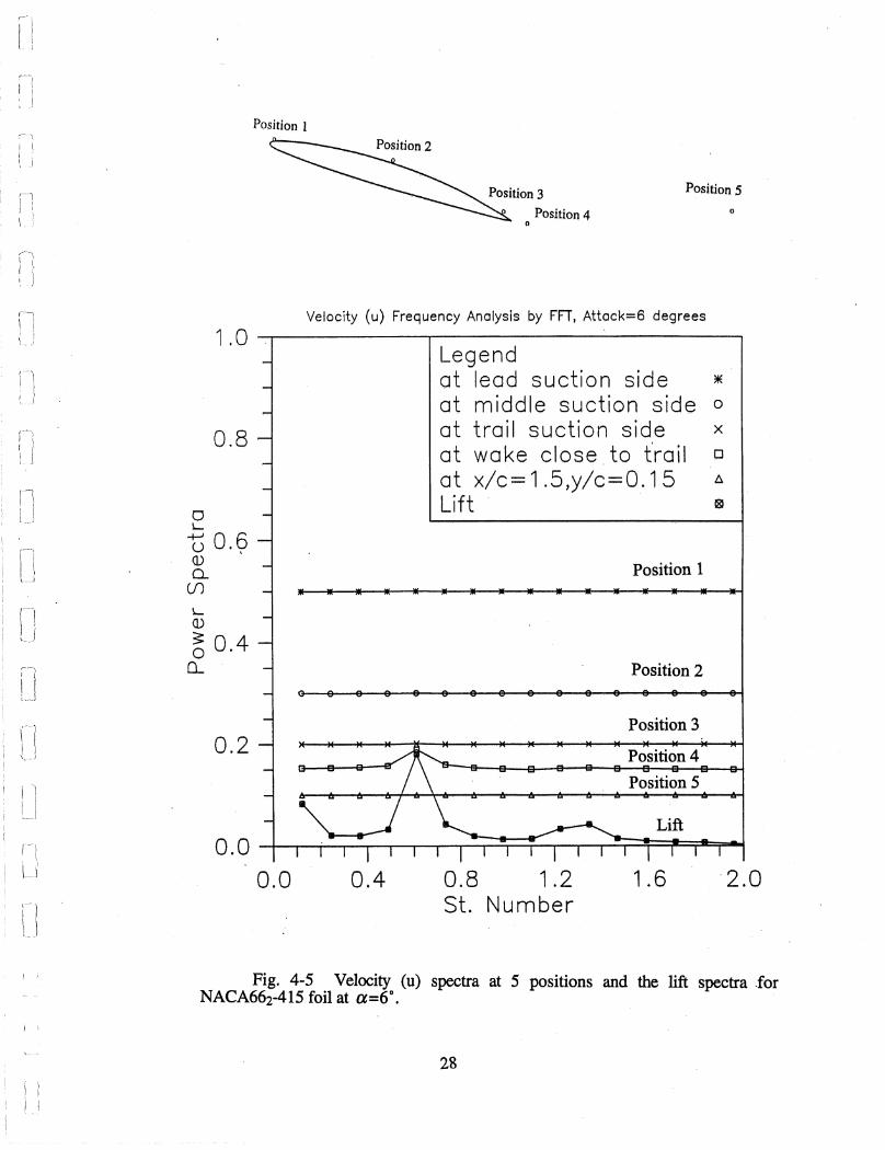
. Velocity (u) spectra at 5 positions and the lift spectra for NACA662-415

foil at 0.=6°.

Instantaneous vorticity component (coz) contours on the mid-span cross­section ofNACA662-415 foil at 0.=10°.

Close-up of the leading edge vortex shedding during one cycle featured by instantaneous vorticity component (coz) contours on the mid-span cross­section ofNACA662-415 foil at 0.=10°.

Velocity (u) spectra at 5 positions and the lift spectra for NACA662-415

foil at 0.= 1 0°.

Instantaneous vorticity component (coz) contours on the mid-span cross­section ofNACA662-415 foil at 0.=15° during one period of stall washout.

Velocity (u) spectra at 5 positions and the lift spectra forNACA662-415

foil at 0.= 15°.

Instantaneous velocity vectors on the mid-span cross-section of NACA662-415 foil at 0.=15°.

Instantaneous vorticity component (coz) contours on the mid-span cross­section ofNACA662-415 foil at 0.=20°.

Velocity (u) spectra at 5 positions and the lift spectra for NACA662-415

foil at a.=20°.

Instantaneous vorticity component (coz) contours on the mid-span cross­section of an E.N. foil at 0.=6.2° under non-cavitating condition.

vi

[I

n 11 I , I :

11 , I I !

r, , I

I 1, L,

o o []

U rJ' L

U [l I !

I I

Fig. 5-2

'Fig. 5-3

Fig. 5-4

Fig. 5-5

Fig. 5-6

Fig. 5-7

Fig. 5-8

Fig. 5-9

Fig. 5-10

Fig. 5-11

Fig. 5-12

Fig. 5·13

Fig. 5-14

Fig. 5-15

Fig. 5-16

Fig. 6-1

Time-averaged velocity field around an E.N. foil at cx.=6.2° under hon­cavitating condition.

Close-up of the velocity field at the leading 'edge of an E.N. foil at cx.::::::6.2° under non-cavitating condition.

Time-averaged pressure coefficient contours around an E.N. foil at (X.::::::6.2° under non-cavitating condition.

Time-averaged pressure coefficient distribution along E.N. foil surface at (1.::::::6.2° under non-cavitating condition.

Instantaneous vorticity component (roz) contours on the mid-span cross­section of an E.N. foil at a=6.2° under cavitating condition of 0'::::::1.2.

Experimental photographs taken by Kubota et al. (I 989) for an E.N. foil at a=6.2° under cavitating condition of 0'=1.2.

Comparison of computed velocity field with experimental result (Kubota et al., 1989) offlow over an E.N. foil at (X.=6.2° under cavitating condition of 0'=1.2.

Instantaneous velocity field around an E.N. foil at a=6.2° under cavitating; 'i,',

condition of 0'=1.2. ',',,"\

Close-up of instantaneous velocity fields at the leading edge of an E.N. foil at a=6.2° 'under cavitating condition of 0"=1.2, featured by one period leading edge vortex shedding due to the cavitation.

Computed time-space (t,y) distributions of vorticity component (roz) at three vertical sections: (a) x/c=0.25; (6) x/c=0.65, (c) x/c=1.05, for an E.N. foil at cx.::::::6.2° under cavitating condition of 0'=1.2.

Measured time-space (t,y) distributions of vorticity component «(i)z) at x/c=1.05 (Kubota et aI., 1989) for an E.N. foil at cx.=6.2° under cavitating condition of 0"=1.2.

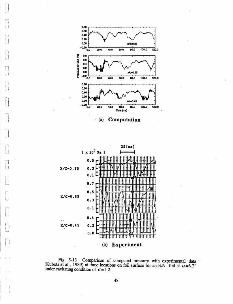
Comparison of computed pressure with experimental data (Kubota et aI., 1989) at three locations on foil surface for an E.N. foil at cx.=6.2° under cavitating condition of 0'::::::1.2. '

Computed long period pressure change with time at five locations on foil surface for an E.N. foil at cx.=6.2° under cavitating condition of 0'::::::1.2.

Comparison of computed normal velocity at x/c=1.25 and y/c::::::0.133 with experimental data (Kubota et aI., 1989) for an E.N. foil at cx.=6.2° under cavitating condition of 0"::::::1.2.

Computed time-averaged pressure distributions on E.N. foil surface at, cx.=6.2° with different cavitation numbers.

Relationship between pressure and density.

vii

Fig. 6-3

Fig. 6-4

Fig. 6-5

Fig. 6-6

Fig. 6-7

Fig. 6-8

Fig. 6-9

Fig. 6-10

Fig. 6-11

Fig. 6-12

Fig. 6-13

Fig. 6-14

Fig. 6-15

Fig.6 .. J6

Fig. 6-17

Fig. 6-18

Comparison of vortex-type cavity appearance onNACA0015 foil at a=20° under cavitating condition of 0"=1.7, (a) experimental photograph; (b) computed density distribution.

Instantaneous. pressure field around NACA0015 foil at a=4° under cavitating condition of 0"=1.5 (moving cavity).

Instantaneous density distribution around NACAOO 15 foil at a=4° under cavitating condition of 0"=1.5 (moving cavity).

Instantaneous vorticity around NACA0015 foil at a=4° under cavitating condition of 0"=1.5 (moving cavity).

Instantaneous pressure field around NACA0015 foil at a=4° under cavitating condition of 0"=1.0 (stable. sheet cavity).

Instantaneous density distribution around NACAOO 15 foil at a=4 0 under cavitating condition of 0"=1.0 (stable sheet cavity).

Instantaneous vorticity around NACAOO 15 foil at a=4 0 under cavitating condition of 0"=1.0 (stable sheet cavity) ..

Instantaneous pressure field around NACAOO 15 foil at a=8° under cavitating condition of 0" = 1. 0 (stable sheet cavity).

Instantaneous density distribution around NACAOO 15 foil at a=8° under cavitating condition of 0" = 1. 0 (stable sheet cavity).

Instantaneous vorticity around NACAOO 15 foil at a=8° under cavitating condition of 0"=1.0 (stable sheet cavity).

Instantaneous pressure field around NACA0015 foil at a=8° under cavitating condition of 0"=1.0 (sheet and cloud cavities).

Instantaneous density distribution around NACAOO 15 foil at a=8° under cavitating condition of 0"=1.0 (sheet and cloud cavities).

Instantaneous vorticity around NACAOO 15 foil at a=8° under cavitating condition of (j ~ 1. 0 (Sheet and cloud cavities r . Instantaneous pressure field around NACAOO 15 foil at a=20° under cavitating condition of 0"=1.0 (sheet and cloud cavities).

Instantaneous density distribution around NACAOO 15 foil at a =200 under cavitating condition of 0"=.1.0 (sheet and cloud cavities).

Instantaneous vorticity around NACAOO 15 foil at a=20° under cavitating condition of 0"=1.0 (sheet and cloud cavities).

Instantaneous pressure field around NACA0015 foil at three span-wise sections at a=8° under cavitating condition of 0"=1.0, (a) left end section (Section 1, NZ=2), (b) mid-section (Section 2, NZ=15), (c) right end section (Section 3, NZ=28) ..

viii

rl II n I I I I iJ

ri I I

I 1 .. 1

'I

U

[l

[J

n

U , II

lJ fl LJ

[J

U [j

lJ []

, I

I I •

I I

. I I \

Fig. 6~19 Instantaneous density distribution around NACAOO 15 foil at three span~ wise sections at q.=8° under cavitating condition, of 0'=1.0, (a) left end section (Section 1, NZ=2), (b) mid~section (Section 2, NZ=15), (c) right end section (Section 3, NZ=28).

Instantaneous velocity field around NACAOO 15 foil at three span-wise sections at cx.=8° under cavitating condition of 0'=1.0, (a) left end section (Section 1, NZ=2), (b) mid~section (Section 2, NZ=15), (c) right end section (Section 3, NZ=28).

Instantaneous pressure field around NACAOO 15 foil at three vertical levels at cx.=8° under cavitating condition of 0'=1.0, (a) foil surface level (Section 1, NY=l), (b) y/c=0.05 (Section 2, NY=9), (c) y/c=O.l (Section 3, NY=15).

Instantaneous density distribution around NACAOO 15 foil at three vertical levels at cx.=8° under cavitating condition of 0'=1.0, (a) foil surface level (Section 1, NY=I), (b) y/c=0.05 (Section 2, NY=9), (c) y/c=O.1 (Section 3, NY=15).

Instantaneous velocity field around NACA0015 foil at three vertica1levels at cx.=8° under cavitating condition of 0'=1.0, (a) foil surface level (Secti()n 1, NY=I), (b) y/c=0.05 (Section 2, NY=9), (c) y/c=O.1 (Section 3, NY=15).

ix

I. INTRODUCTION

Traditionally, cavitating flows are regarded as two-phase flows and fundamentally different from non-cavitating flows. Thus, classical works of Helmholtz (1868) and Kirchhoff (1869) neglect the density of the gas and treat cavitating flows as free'-surface potential flows of the . liquid phase. This tradition has been extended for about a century by numerous investigators, such as Riabouchinsky(1919), Wu (1956), and Tulin (1958), to name a few. The most serious problem limiting the progress of the free-surface potential flow approach is the need for a cavity closure condition for finite length cavities to approximate the real fluid flow phenomenon. Different closure models have been proposed by a number of researchers, SU9h as the image model (Riabouchinsky, 1919), the re-entrantjet model, the transition model (Wu, 1956), the singularity model (Tulin, 1958), and the open cavity model (Song, 1965). The free-surface boundary value problem can also become unmanageably complex when there are many cavitation bubbles or when a cavity is highly unstable.

To overcome the difficulty presented by the unsteady and multiple free surfaces, Kubota et al. (1992) proposed a "bubble two-phase flow model" based on an assumption that the fluid consists of a bubble-water mixture; and the bubble volume change is governed by a modified Rayleigh's equation. In this way the existence of cavitation is inferred by the existence of a large void fraction region. An ingenious idea--and they were able to qualitatively mimic the appearance of unsteady sheet and cloud cavities. However, the paper gives no quantitative comparison with experimental results. Combining the ideas of Kubota et al. with Song and Yuan's (1988) weakly compressible fluid, a simpler single-phase cavitating and non-cavitating flow model can be produced.

The weakly compressible flow (also known as compressible hydrodynamic flow) model is based on the assumption that the equation for state of water can be approximated by a linear equation relating pressure and density. Recently Song (1996) and Song and Chen (1996) showed that the weakly compressible flow equations contain the inner solution (compressibility boundary layer flow) and the outer solution (incompressible flow) under small Mach number conditions. Furthermore, the outer solution is independent of the sound speed used in the model; therefore, an incompressible flow solution can be obtained with greatly increased speed. This approach is now further extended to include a more general equation of state that approximates the pressure­density relationship extending from the liquid phase to the gas phase. The linear relationship is still assumed for the liquid phase, but the gas phase is represented by a function that makes the density decrease very rapidly when tv.e pressure falls below a specified critical pressure. The fully compressible flow equations of continuity and

1

r' . I I •

\1

(-,

I i I i \ !

momentum are used for the gas phase, but all quantities are continuous at the gas~liquid interface.

This new single phase unsteady three-dimensional flow model with a complex equation of state is applied to: 1) a non-cavitating flow about a two-dimensional foil, 2) an R.N. (Elliptic Nose) foil with sheet and cloud cavitation, and 3) a NACA0015 foil with and without cavitation. Quantitative as well as qualitative comparisons with experimental data are made and good agreements are obtained.

2

II. THEORETICAL CONSIDERATIONS

The importance of compressibility has long been overlooked by most hydrodynamicists. But, much like the fact that viscosity cannot be ignored in the viscous (space) boundary layer, Song (1996) has shown that the compressibility cannot be ignored in the compressibility (time) boundary layer. The fundamental characteristics of the equations of motion change when the viscous terms are dropped. Similarly, the characteristics of the equation of continuity changes when the fluid is assumed to be incompressible and the time derivative term is dropped. Therein lies the fundamental difficulty in representing the real fluid flows with the classic hydrodynamic equations, no matter how large the Reynolds number or how small the Mach number. The remedy proposed by Song and Yuan (1988) is to assume the flow to be IIbarotropic li rather than incompressible, and write the equation of state as

where a is the speed of sound.

iP=d­op

The equation of continuity can now be written as

iJp + V .pel-v =pv .Vd­Ot

(1)

(2)

For weakly compressible flow, the speed of sound is assumed to be constant, hence, the density is a linear function of pressure. In this case, the right-hand side of Eq. (2) is zero and the equation of continuity simplifies to

(3)

where the subscript "0" represents a reference quantity. Note that both Eqs. (2) and (3) are written in conservative form--one with and the other without a source term.

For a cavitating flow problem, it is necessary to simulate at least approximately the vaporization phenomenon. To simulate a rapid change in density below the critical pressure, the following equation is selected for the equation of state,

3

i

r-I i I I I

ii I

I

L

5 . p= L4P'

;=0 for Pe <P <Pc (4)

The above equation is joined by the following equation at the upper end,

for Pc<P (5)

and joined by the following equation at the lower e~d.

p=Bp, for P<Pe (6)

The coefficients are so adjusted that the resulting pressure~density curve has a desirable shape.

Since the Mach number of the flow inside a cavity may not be small, it is prudent to use the equations of motion for fully compressible fluid to simulate the flow inside the cavity. The equations of continuity and motion may be written in a conservative form as follows.

F=iE+ jF+kG (7)

where S is source which mayor may not exist and i, j, k are the unit vectors in x, y, and z directions, respectively. The functions U, E, F, G, and S are defined in the following.

U = [p,pu,pv,pw]T (8)

(9)

(10)

(11)

[ - 2 ]T S = pV. Va ,0,0,0 (12)

4

III. NUMERICAL ApPROACH

The finite volume approach with MacCormack's (1969) predictor· corrector method has been used with good results. Equation (7) is first integrated over a computational finite volume and divided by the volume. In the process, the volume integral of divergence is converted to the surface integral by applying the divergence theory. The resulting equation is

au I - -- +-J M F .lidA = S a ,1V (13)

In the above equation bar means volume averaged quantity, A is surface area, and ii is the unit normal vector on the surface of integration. Since the quantities to be calculated are always the volume averaged values, the superscript bar will be dropped hereafter. The above equation is a simple statement of the law of conservation where the rate of increase

of U in a volume is equal to the net influx of F plus the source S. Thus, Eq. (13) can be discretized with any standard finite difference scheme. A detailed description of the process used herein is described by Yuan (1988).

Since a finite volume approach can resolve only the quantity of scale larger than the finite volume used, it is necessary to use a closure model for turbulent flow simulation. A simple Smagorinsky (1963) subgrid scale turbulence model is used. This model assumes that the shear stress tenser 'r;j can be calculated by adding an eddy viscosity Vt

to the kinematic viscosity v. Smagorinsky proposed the following equation for the eddy viscosity.

(14)

In the above equation C is a coefficient to determined and ,1 is the size of the finite volume. Experience indicates that a C distribution which is zero on the wall and increases to 0.12 outside of the boundary layer generally gives satisfactory results.

The size of the finite volume used is often too large to adequately resolve the sharp velocity gradient near a solid wall. For this reason a wall function or a partial slip condition (becomes non· slip when boundary layer is thick) -is used; see He and Song (1991) for a description of this condition. Because the cavity is assumed to be a

5

lJ

: .. / , I l-"

I I

continuous extension of the liquid, no free surface boundary condition is necessary. Only the hydrodynamic quantities are of interest (acoustics are ignored); therefore, an arbitrarily large value ofM=O.4 is chosen for the liquid part of the flow to speed up the compu,tation. Recall that the outer solution of the weakly compressible flow equation is independent of M and is the incompressible flow.

6

IV. Non-Cavitating Flow Over A Foil

Flow over a hydrofoil even at non-cavitating conditions generates a very complicated unsteady flow phenomena similar to those found in two-dimensional diffuser flow with different diffusion angle, especially at large angle of attack. At a small angle of attack, the flow separation may occur at the trailing edge, and the unsteady characteristics of the flow are dominated by the trailing edge vortex shedding much like the unsteady shear-layer flow. As the attack angle increases, the unsteady separation point on the suction side moves upstream. At a large enough attack angle, the separation may occur near the leading edge, and a periodical vortex shedding like the well-known Von Karman's vortex shedding from a bluff body may take place. However, in some cases, a number of vortices may accumulate near the foil before one large and strong negative vortex is washed out. Each negative vortex being washed out induces a positive vortex at the trailing edge which is also washed out, thus, generating a low-frequency oscillation.

The vortex shedding and vortex washout phenomena described above are simulated using this model, and the results are presented in this section. The main effort of the non-cavitating flow study is focused on the unsteadiness of the flow at different attack angles. The computed mean pressure distribution on the foil agrees very well with the experimental data. Most of the unsteady characteristics found in previous experiments are also successfully simulated.

4-1 Previous Studies

Numerous experiments and numerical studies of the flow over a foil at non­cavitating conditions have been carried out for several decades, and a good understanding of general flow patterns has been achieved. The progress and the state-of-the-art on the subject can be learned from a number of review papers (McCroskey, 1982; Carr, 1988; and Doligalski et at, 1994). However, some important flow characteristics, such as the dynamics of stall vortex and unsteady flow structures, are still far from being completely understood. Also a systematic and detailed study on how the unsteady stall phenomena are affected by the attack angle change is lacking. For example, Zaman et al. (1989) observed the occurrence of low frequency oscillations of velocity and lift when the flow approaches the stalling condition. But some questions related to the low frequency oscillation phenomenon remain unanswered due to insufficient experimental data. Because of its importance to rotor craft, low frequency stall received extensive experimental studies in recent years by Acharya and Metwall (1992), Currier and Fung

7

-, I I

Ii

I: I (

l 1

,-I (.

, I I' I " ,. __ J

II L.J

;'\ I . U

(1992), and Chandrasekhara et al. (1993). The low frequency stall frequently that occurs with a pitching foil has also been found to occur in some cases around a stationary foil.

The numerical model described above can be used with both cavitating and non­cavitating flow cases. In fact, when the cavitation number is set to a very large number, the flow becomes non-cavitating flow. In this section, the numerical model is used to simulate the flow over a stationary foil at different attack angles under non-cavitating flow conditions. The objectives of the non-cavitating flow study are: 1) demonstrating how the unsteadiness of the vortex generation process is affected by the attack angle; 2) revealing more details of the dynamic stall process by means of numerical visualization; 3) providing the bases for comparing and facilitating a further understanding of cavitating flow around hydrofoils.

4-2 Model Validation

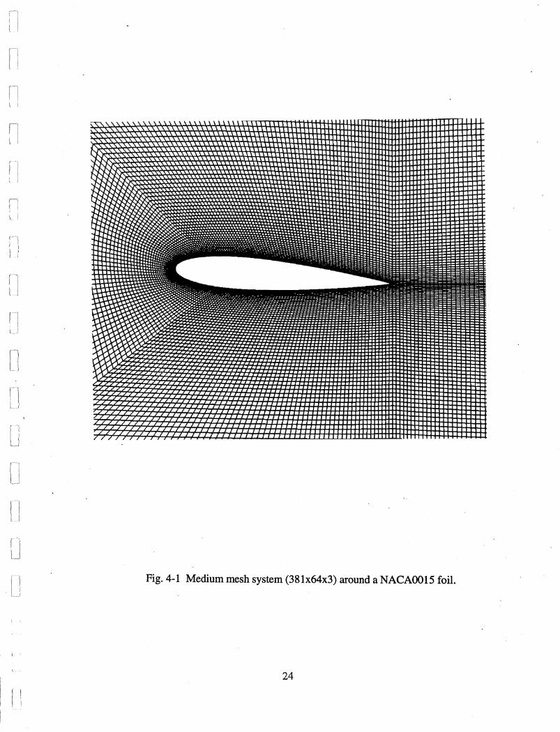
Very small Mach number flow or a weakly compressible flow is considered, and p and a in Eqs. (8-12) are set equal to constants. A body-fitted grid system is used to ensure accuracy. To assure that the computed results will be grid independent, three mesh systems (191x32x3, 381x64x3, 761x128x3) were tested. This model contains only three", grid points in the spanwise direction so that basically two-dimensional flow is represented. Part of the medium mesh system (381x64x3) around the NACA0015 foil is shown in Fig. 4-1. It was found that the medium mesh system is fine enough to resolve the large-scale unsteady structures, Therefore, the results discussed in this report are based on medium mesh for comparison purposes unless otherwise indicated. The Reynolds number used in the compution is 105,

The numerical model was first tested on NACAOO 15 standard foil, which has been intensively studied by Izumida et al, (1980) and Kubota et al. (1992) by experiment and computation under cavitating and non-cavitating conditions. Fig. 4-2 shows the comparison of the computed time-averaged pressure distribution on the foil surface with the experimental data of Izumida et al. for attack angle (a) of 0, 4, and 8 degrees. The experimental data were taken only on the suction side. As the figure indicates, the computed results agree very well with the experiments. The computed lift coefficients at three attack angles are 0.0, 0.474, and 0.905, respectively.

To test the effect of the grid size, three mesh systems (191x32x3, 381x64x3, and 761x128x3) wer.e used for the case of a =8°. The time-averaged pressure distributions based on the three meshes are shown in Fig. 4-3. It appears that the results using the medium size mesh are very close to those using the fine mesh. Since the fine mesh takes more than eight times the work to generate the same results than the medium mesh system, the computed results discussed below are all based on the medium mesh system.

8

4-3 Unsteady Structures

A non-symmetrical foil NACA662-415 was chosen for the unsteady flow. study.

Four different attack angles 6°, 10° , 15° , and 20° were selected for the study. Results showed that the flows at these attack angles represent different unsteady flow regimes. These flow regimes are very similar to the flow regimes in two-dimensional symmetrical diffusers of different diffusion angles, as found experimentally by Fox and Kline (1962) and computationally by He and Song (1991).

4.3.1 Trailing edge unsteadiness (a=6 0)

At this small attack angle the flow separates near the trailing edge on the suction side, which results in unsteady vortex shedding from the trailing edge. The separation point moves upstream as the attack angle increases. Fig. 4-4 shows instantaneous vorticity contours during one period of the trailing-edge vortex shedding. In the other region away from the trailing edge, the flow is steady, and there is no leading edge separation.

Fig. 4-5 shows the power· spectra·of lift and velocity component (u) recorded at five positions, as sketched at the top of the figure. As the figure indicates, only the lift and the velocity in the wake near the trailing edge (position 4) show the unsteadiness due to the trailing-edge vortex. shedding. The Strouhal number (fc-sin alU) of the wake oscillation is 0.60. This flow regime corresponds to the steady flow regime of the two­dimensional diffuser at a 6° diffusion angle (see He and Song, 1991).

4.3.2 Leading edge separation (a= J 0 0 )

When the attack angle is about 10°, the leading edge separation occurs, which generates a leading edge separation bubble (clockwise rotating eddy). Vorticity generated at the separation point continuously feeds the· eddy, causing the eddy to grow in size and intensity. When the eddy grows·· to a certain size, part detaches and forms a primary dynamic stall vortex. Such a process of vortex generation and detachment is similar to bluff-body vortex shedding.· The detached· vortex moves downstream with the main flow (U) at an approximate speed (Doligalski et aI., 1994),

k V =u--

c 2d (15)

where k is the vortex strength, and d is the distance from the center of the vortex to the foil surface. Due to the relatively small vortex strength, the speed of vortex convection is not much different from that of the main flow.

Fig. 4-6 shows the instantaneous vorticity contours during one period of the vortex shedding at 0..= 10°. The detached vortex remains very close to the foil surface

9

~,

I I

:1

il

! \ I

:1 . ,

LJ

n .; 1 I~,

[1 U

(l \

Ll

i'l L.

I I., " J

I I iii

while being transported from the leading edge to the trailing edge. When this clockwise rotating vortex reaches the trailing edge, it induces a counterclockwise rotating vortex at the trailing edge. Four instantaneous close-up views of the leading edge vortex within one cycle of shedding is shown in Fig. 4-7.

Fig. 4-8 shows the power spectra of lift and the velocity component (u) recorded at the same five positions, as stated above. The most significant spectral peak in the figure is at the leading edge, where the unsteadiness due to the vortex shedding is very strong. The Strouhal number (f·c'sin aJU) of the leading edge vortex shedding is 0.2. This flow regime corresponds to the small transitory stall regime of two-dimensional diffuser at a 13 0 diffusion angle.

4.3.3 Large vortex washout (a=J5°)

As the attack angle increases, the shed vortex becomes stronger, and its moving speed decreases according to Eq. (15). At this large attack angle, a vortex merging and washout phenomenon take place. A vortex that was shed earlier moves slowly and appears to wait for the trailing vortices to catch-up and merge, resulting in a large vortex in the vicinity of the foil. This large combined vortex is eventually washed out of the foil .' region into the wake. The large stall washout generates strong, low frequency oscillatory lift and drag. .

Fig. 4-9 shows 'one period of combined vortex washout featured by the instantaneous vorticity contours at cx.=15°. In Fig. 4-9(a), one large stall vortex is washed out from the foil. The vortex at the trailing edge in this figure is induced by the large clockwise stall vortex. Hence, the induced small but high strength vortex at the trailing edge at this stage is a counterclockwise vortex. In the leading edge region, as more shed vortices shed and merge, the combined vortex becomes larger and larger. Since the large vortex moves downstream slowly, the new shed vortices from the leading edge can still catch up before it reaches the trailing edge. This flow regime corresponds to the large transitory stall of the two-dimensional diffuser of 18° diffusion angle (He and Song, 1991). Such a vortex structure and its unsteady behavior are also very similar to the coalescence of vortex cavitation observed in a water tunnel experiment using high-speed photograph (Kubota, et al., 1992). In fact, a recent study (Song, et aI., 1997) to be described later shows that the cavitation-induced unsteady flow structure over a foil at a small attack angle is similar ,to that of non-cavity flow at a larger angle.

At the saine five positions as before, the instantaneous velocity component (u) and lift were recorded. Their power spectra are shown in Fig. 4-10. Due to the larger leading edge separation eddy, Position 1 falls inside of the eddy and has very little velocity fluctuation. In contrast, Position 2 is close to the end of the separation eddy and has strong oscillation ofthe leading eddy shedding frequency (fl·c·sin aJU=0.17). At Position

5 (near wake region) the low frequency large eddy washout (f2·c·sin aJU=0.05) is more significant. An interesting feature is that the unsteady lift contains two dominant

10

frequencies: the low washout frequency 'and a higher frequency (:£3 oeosin cx/U=0.3). The higher frequency unsteadiness is found to' be related to the trailing edge secondary vortex shedding similar to that at low angle of attack. The unsteadiness of the leading edge vortex shedding does not contribute much to lift oscillation because there is more than one such vortex on the foil, and their effect on lift cancel out each other.

Fig. 4-11 shows the details of the leading edge vortex shedding featured by the velocity vectors. The unstable large recirculation at the leading edge is clearly· seen. The complex flow structure contains the spike-like eruption, shear . layer roll-up, and viscous­inviscid interaction, as described by Doligalski etal. (1994), and visualized in experiments by Acharya and Metwally (I 992}. A similar low frequency, combined eddy washout phenomenon was also found in an experiment by Zaman et al. (1989). The shedding vortex accumulation on the foil surface is also very similar to the cavitation coalescence found in experiments using high-speed photographs (Kubota et al., 1992).

4.3.4 High attack angle stall (a=200)

As the attack angle is increased further; the shed vortex from the leading edge is more detached from the foil surface. As a result,the vortex'merging becomes'less significant. The extreme case is cx.=90°, in which case the only large-scale unsteadiness is the bluff-body vortex shedding.

Fig. 4-12 shows one period of the leading-edge vortex shedding featured by the instantaneous vorticity contours at cx.=20°. The power spectra of u at the five positions and the lift are 'displayed in Fig. 4-13. It is seen that the unsteady flow velocity at all five positions are, dominated by the leading-edge vortex shedding, which has a Strouhal Number (focosin cx./U) of 0.17, although large eddy washout can still occur from time to time. In this case, the lift power spectrum shows a small peak representing the'leading­edge vortex shedding.

In summary, the above discussed four cases represent four flow' regimes of flow over a hydrofoil at different attack angles. Each regime features different large-scale unsteady structures. The flow regimes are very similar to those found in a two­dimensional diffuser flow with different opening angle (Fox and' Kine, 1962; He and Song, 1991). ,

11

;"1 ,\

. i \ _ J

fl II

I I

v. CAVITATING FLOW OVER A THIN FOIL

As mentioned before, flow at a cavitating condition is much more complicated than the corresponding non-cavitating flow. Not only do cavity generation and collapse lend difficulties for numerical simulation, but there are more factors to be considered. In the current cavitating flow study, two types of foil shapes were examined: the NACAOOl5 which represents a typical thick foil (thickness ratio of 12%); and the R.N. (Elliptic Nose) foil which is a relatively thin foil. The cavitating flow results over the NACAOO 15 foil will be discussed separately in the next section since different phenomena were observed. In this section, the cavitating flow results over an E.N. foil is analyzed.

It is known that during non-cavitating conditions, the separation point at the suction side of a thick foil moves upstream to the half foil chord as the attack angle increases before the leading edge vortex shedding occurs. However, for a thin foil, the leading edge vortex shedding occurs at a relatively small attack angle due to the high peak negative pressure at the leading edge. The so-called E.N. foil is a symmetrical hydrofoil with a thickness ratio of 8%. The foil geometry can be expressed as (Kawanami et aI., 1996),

y = +(0.05746 x - 0.06079)

Y = ±~~x(0.6 - x) 15

(0.4187 :s; x :s; 1.0)

(0 :s; x :s; 1.0)

(16)

(17)

The other reason to study this foil is that an extensive experimental study on cloud cavitation around this foil and its unsteady structures were reported by Kubota et al. (1989). Recently, Kawanami et al. (1996) reported a follow-up study of this foil about the mechanism and control of cloud cavitation. In order to compare the modeling results, conditions were set to be the same as those used in their experiments.

The same mesh system used for the non-cavitating flow computation was used. To compare the experiments, an attack angle of 6.2 degrees was used in the computation, but different cavitation numbers were tested.

5.1 Non .. Cavitating Flow Results

As the basis for comparison with cavitating flow characteristics, non-cavitating flow at the same modeling configuration was first simulated. it was found that the flow

12

field over the E.N. foil at the attack angle of 6.2 degrees at non-cavitating conditions is mostly steady except for the unsteady vortex shedding at the trailing edge.

Fig. 5-1 shows one period of the vortex shedding at the trailing edge featured by the vorticity contours. As indicated in the figure, the shed vortices from the trailing edge gradually defuse in the wake region. There is no separation at the leading edge. Fig. 5-2 shows the time-averaged velocity vectors. No boundary layer separation except at the trailing edge is shown. The close-up of the velocity vectors at the leading edge is shown in Fig. 5-3, The time-averaged pressure coefficient distribution around the foil is shown in Fig. 5-4. Fig. 5-5 displays the pressure coefficient distribution on the foil surface. At the leading edge, there is a sharp negative pressure peak higher than 4. The sharp negative peak is typical in a thin foil like this. The computed time~averaged lift coefficient at this attack angle (6.2°) is 0.754.

5.2 Cavitating Flow Results

At cavitating conditions under the same attack angle (a=6.2°) the flow patterns are totally different from those of the non-cavitating flow. When the ambient pressure is lowered below the critical value, cavitation starts in the leading edge region due to the peak negative pressure at the leading edge. The cavitation bubble exhibits a distinctively periodical behavior, alternating between the growth stage and the break-up stage. During the growth stage, vorticity is continuously produced near the leading edge and fed into the bubble making the bubble grow and form a large sheet cavity. The sheet cavity is relatively stable during the growth stage. But it becomes unstable and breaks away from the upper section and forms a large clockwise rotating free eddy. Actually, this free eddy is highly turbulent and contains numerous small cavitating eddies called "cloud cavitation."

Fig. 5-6 shows one cycle of the cloud cavitation featured by instantaneous vorticity contours when the cavitation number is about 1.2. In Fig. 5-6(a), a large sheet cavity is still growing as one cloud cavitation has just been washed out away from the foil ' s trailing edge. In Fig. 5-6(b), a large portion of the sheet cavity is beginning to break away at about the 1/4 chord point. In Fig. 5-6 (c) the sheet cavity that has broken away turned into a full fledged cloud cavity and moved to about the 3/4 chord point where relatively high ambient pressure is causing the cloud cavity to start collapsing. From Fig. 5-6( d) to Fig. 5-6(e), the collapsed cloud cavitation is gradually dying out as it is washed away from the foil section, while another sheet cavity is forming. This completes one cycle of sheet cavity growth--break-up into cloud cavity--collapse and washout of cloud cavity. This same periodical characteristics of sheet and cloud cavitation was observed in experiments by Kubota et al. (1989). Fig. 5-7 shows the photographs of one period of the cavitation cloud from generation to washout, taken from the experiment by Kubota et al. (1989). Although Fig. 5-6 and Fig. 5-7 show flow visualization using different physical quantities, the flow patterns shown are strikingly similar. The computed velocity field also illustrates the same unsteady characteristics as shown in Fig. 5;..8(a). Similar velocity measurements during one cycle of cloud cavitation based on LDV measurements of Kubota et al. are

13

il , )

n I I, t,

Cl I I,

:,' I

[l \

'i i

l J

r­'L I

n Ii I ,I , j I.

, I

I I l

shown in Fig. 5-8(b). It appears that the large-scale unsteady structure of the cloud cavitation obtained by the computational model agrees very well with the experimental results. Compared with the non-cavitating flow shown in Fig. 5-1, cavitating flow is. much more unstable. But there are many similarities when compared with the non-cavitating flow at an attack angle of 15° where vortex shedding and washout occur as shown in Fig. 4-9.

The velocity vectors around the foil at the moment when the sheet cavity begins to break away from the foil's upper section, corresponding to Figs. 5-6(c), is shown in Figs. 5-9. This figure indicates the three different vortex structures as mentioned above. They are the leading edge vortex production which takes place in the first 10% of the foil section (between points 1 and 2), the large sheet cavity which extends to 25% of the foil (between points 2 and 3), and the cavitation cloud which moves from the foil's middle section to the wake (downstream of point 3). The highly unsteady leading edge vortex production zone should probably be regarded as a part of the sheet cavity structure. Fig. 5-10 shows the close-up of the velocity field in the vorticity production zone (between points 1 and 2) during one cycle of oscillation.

Time-space (t,y), distributions of vorticity at three sections (x/c=0.25, 0.65, 8lld:, 1.05) are shown in Fig. 5-11. At x/c=0.25, Fig. 5-11(a), the vorticity contour lines are nearly parallel to the t-axis, indicating that the sheet cavity'is relatively stable. Periodically near the time of break up, the contour lines become normal to the time axis, indicatiIlg rapid change. At xlc=0.65 as shown in Fig. 5-11(b), the large vortex structure of cloud cavitation appears periodically. After each cloud cavitation with negative vorticity passing this foil section, a small positive vortex structure is induced. In Fig. 5-11(c), located 0.05c downstream of the trailing edge, the vortex of cloud 'cavitation becomes weaker. Positive vorticity induced by the flow on the pressure side is present near y = 0 most of the, time. Therefore, the vorticity distribution at this wake section changes from negative in the upper level to positive in the lower level. The computed vortex structure at the wake section was also recorded in Kubota et a1.'s experiment (1989) using LDV. Fig. 5-12 shows the experimental results.

Fig. 5-13 (a) shows the computed pressure fluctuations recorded at three locations (xlc=0.45, 0.65, and 0.85), respectively. At x/c=0.45 as shown in Fig. 5-7(a), the high frequency pressure oscillations with sharp cut-off at p = 0 represents the sheet cavity pressure fluctuations. At x/c=0.85 as shown at the top of Fig. 5-13(a), the pressure fluctuation reflects mostly' the change due to the cloud cavitation. The computed frequency is about 23 Hz and the maximum pressure coefficient is about 0.58xl0E5 Pa. The measured pressure data at the same locations (Kubota et al., 1989) are shown in Fig. 5-13(b). The measured frequency is 25.4 Hz and the ma;ximum pressure coefficient is about 0.52xl0E5 Pa.' The agreement between the computation and the experiment is surprisingly good. For a longer time period, the pressure change with time at five locations along the foil surface is shown in Fig. 5-14. At xlc=O.25, high frequency oscillation of the sheet cavity is predominant, but the dominant frequency gradually decreases as X/C increases. At x/c=1.05, the pressure fluctuation is fully dominated by the

14

large-scale cavitation cloud. The computed normal velocity at xlc=O.25 near the foil surface (y/c==OJ33) is shown in Fig. 5-15(a). The corresponding data ofI<.ubota et aI.are shown in Fig. 5 .. 15(b).

Fig. 5-16 shows the computed time-averaged pressure distribution on the foil surface at different cavitation numbers compared with that of non-cavity flow. As the cavitation number decreases, the flat pressure zone on the suction side, which represents the vapor pressure, becomes longer, indicating that the cavity is getting longer.

15

~

I I

Ii L_I

[J

u

I I \

VI. CAVITATING FLOW OVER A THICK FOIL

As noted before, the cavitation characteristics of a thick foil are somewhat different from those of a thin foil. The location of cavitation occurrence varies more with the attack angle and the phenomenon of sheet cavity breakdown, leading to less predictability of cloud cavitation. In this section, cavitating flow results over a typical thick foil NACAOO 15 are presented. The same mesh system described previously was also used in this case to study the basic characteristics of the cavitating flow. In addition, the number of grids in the spanwise direction has been increased from 3 to 15 and then to 30 to study the three-dimensionality of the flow.

As shown before, non-cavitating flows over a NACAOO 15 foil with various attack angle were simulated first to check for the accuracy of the model as well as to serve as a reference. The comparison of computed pressure coefficient distribution on the foil surface and the experimental data was shown in Fig. 4-2. Good agreements have been noted. Fig. 6-1 shows the pressure-density relationship in the gas phase. Note that the critical pressure coefficient of 0.10 can be chosen arbitrarily. This figure shows a rapid drop of density to 10 % of water within the pressure coefficient drop of 0,01, which is substantially milder than the real vaporization process. But the numerical results of cavitation phenomenon appear insensitive to this curve. The equation of state for Cp > 0.10 is assumed to be linear and matches this curve at the critical point.

6.1 Comparison with Experiments

Only a high speed photograph of cavitating flow at a 20 degree attack angle and the cavitation number of 1.7 published by Kubota et al. (1992) is available for comparison for this foil. Fig. 6-2 (a) is the photograph of the cavitating flow in a water tunnel. and Fig. 6-2 (b) is the corresponding computed instantaneous density distribution. Here the cavitation zones indicated by the relative density less than one are painted white and the non-cavitating zones are shown in black. Small amounts of sheet cavitation near the nose and a larger cloud cavitation away from the trailing edge are captured both experimentally and computationally; they show striking similarities.

16

6.2 Qualitative Description of Two-Dimensional Cavity Flows

6.2.1 Moving and fixed (sheet) cavitation at small attack angle

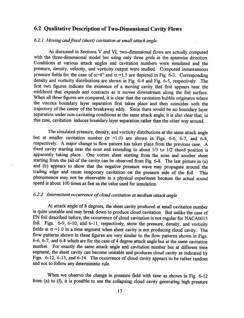
As discussed in Sections V and VI, two-dimensional flows are actually computed with the three-dimensional model but using only three grids in the spanwise direction. Conditions at various attack angles and cavitation numbers were simulated and the pressure, density, velocity, and vorticity output were studied. Computed instantaneous pressure fields for the case of cx.:=4° and cr =1.5 are depicted in Fig. 6-3. Corresponding density and vorticity distributions are shown in Fig. 6 .. 4 and Fig. 6-5, respectively. The first two figures indicate the existence of a moving cavity that first appears near the midchord that expands and contracts as it moves downstream along the foil surface. When all three figures are compared, it is clear that the cavitation bubble originates where the viscous boundary layer separation first . takes place and then coincides with the trajectory of the center of the breakaway eddy. Since there would be no boundary layer separation under non-cavitating conditions at the same attack angle, it is also clear that, in this. case, cavitation induces boundary layer separation rather than the other way around.

The simulated pressure, density, and vorticity distributions at the same attack angle but at smaller cavitation number (cr =1.0) are shown in Figs. 6-6, 6-7, and 6-8, respectively. A major change. in flow pattern has taken place from the previous case. A fixed cavity starting near the nose and extending to about 1/3 to 1/2 chord position is apparently taking place. One vortex sheet starting from the nose and another sheet starting from the tail of the cavity can be observed from Fig. 6-8. The last· picture in ( a) and (b) appears to show that the negative pressure wave may propagate around the trailing edge and cause temporary cavitation on the pressure side of the foil. . This phenomenon may not be observable in a physical experiment because the actual sound speed is about 100 times as fast as the value used for simulation.

6.2.2 Intermittent occurrence of cloud cavitation at medium attack angle

At attack angle of 8 degrees, the sheet cavity produced at small cavitation number is quite unstable and may break down to produce cloud cavitation. But unlike the case of EN foil described before, the occurrence of cloud cavitation is not regular for NACAOO 15 foil. Figs. 6-9, 6-10, and 6-11, r~spectively, show the pressure,density, and vorticity fields at cr = 1. 0 in a time segment when sheet cavity is not producing cloud cavity. The flow patterns shown in these ,figures are very similar to the flow patterns shown in Figs. 6-6, 6-7, and 6-8 which are for the case of 4 degree attack angle but at the same cavitation number. For exactly the same attack angle and cavitation number but at different time segment, the sheet cavity can become unstable and produces cloud cavity as indicated by Figs. 6-12, 6-13, and 6-14. The occurrence of cloud cavity appears to be rather random and not to follow any deterministic rule.

When we observe the change in pressure field with time as shown in Fig. 6-12 from (a) to (t), it is possible to see the collapsing cloud cavity generating high pressure

17

'l l , n I I

r' i I I I

n 11 I I

n

11 u

r~ U

o lJ

[J

u u I I

I I I

I l __ •

I

! ! I ! .

concentration near the 1/3 chord position as indicated by a dark area. This pressure is far above the stagnation pressure, indicating the dynamic and compressibility effect of a

. collapsing cavity. From (d) to (f), it is possible to observe the propagation .of the compression wave away from the center of the collapse. This pressure wave is not quantitatively accurate because the sound speed used in the computation is only about 100th of the real sound speed.

6.2.3 Continuous occurrence of cloud cavitation at large attack angle

At large attack angle and low cavitation number, even a thick foil as the NACA 0015 will continuously produce cloud cavitation or supercavitation. The instantaneous patterns of pressure, density and vorticity for the case of p=20° and cr =1.0 are shown in Figs. 6-15,6-16, and 6-17, respectively.

6.3 Three Dimensionality of Cavitating Flow

To study the three dimensionality of the flow the finite span equal to a 0.7 chord length was selected and the span was divided into 30 equal grid intervals. A nonslip boundary condition was used to simulate a typical water tunnel testing condition. Only,', the results for the case of an 80 attack angle and a cavitation number of 1.0 at an instant' when cloud cavity exists are presented here.

Fig. 6-18 shows the pressure distribution over three different cross-sections: one near the left wall, one at the center of the span, and the other near the right wall. The pressure patterns are very different, and the collapsing cloud cavity condition can be seen only near the right wall at this instant. The corresponding density distribution is shown in Fig. 6-19; the velocity distribution is shown in Fig. 6-20.

Fig. 6-21 shows the pressure distributions over three surfaces roughly parallel with the foil suction surface but at different distances away from the foil. This figure again clearly shows that the cavity collapse occurs near the right wall and near the foil surface. The corresponding density distribution and velocity distribution are shown in Figs. 6-22 and 6-23. Note that the upstream half of Section 1 in Fig. 6-23 is the foil surface and the velocity is zero according to the boundary condition. A wavy vortex pattern in the span direction is a typical flow pattern over a finite span foil with or without cavitation.

18

r \

VII. CONCLUSIONS

The Compressible Hydrodynamic Approach previously developed for large Reynolds number - small Mach number flows has been extended and applied to cavitating and non-cavitating flows about hydrofoils of different shapes at different attack angles and for different cavitation numbers. The unifying factor between the previous approach and the extended approach as well the difference between the present approach, the incompressible flow approach, and the fully compressible flow approach is in the assumption regarding the equation of state. The compressibility characteristics represented by the equation of state directly affect the property of the equation of continuity in much the same way the assumption on viscosity affects the equation of motion. The concept of compressibility boundary layer greatly speeds up the computation of small Mach number flows making it feasible to solve complex problem with currently available computers. The large eddy simulation concept is also incorporated here in order to efficiently simulate the dynamics of large scale eddies. Specific conclusionsconceming non-cavitating flows and their relationships with cavitating flows are listed below.

1. When the cavitation number and the Reynolds numbers are both large, the non­cavitating flow pattern depends greatly with the attack angle. For small angle of attack there is likely to be no boundary layer separation, or the boundary layer separates only at the trailing edge. The separation point is likely to move upstream as the angle of attack is increased.

2. At modest angle of attack, the boundary layer may breakup and produce large­scale vortex shedding. This shedding ·is quite periodic if the foil is thin and the· separation point is fixed at the leading edge. At a larger attack angle, two or more shed eddies may merge near the trailing edge of the foil producing a larger and stronger eddy . This eddy washes out more or less periodically at substantially lower frequencies than vortex shedding.

3. Lift and drag o~cillations due to 'vortex washout and the wake instability are quite significant.. In contrast, vortex shedding generates relatively weak oscillations. This is due to the fact that there are multiple eddies distributed on the foil surface, and their effect on forces cancel each other out.

4. The vortex shedding and washout phenomena of hydrofoil are very much similar to the shedding and washout phenomena of the two-dimensional straight diffuser.

5. For a thin foil like the E.N., cavitation is likely to start at the leading edge. The resulting cavitation is quite periodical and predictable. Vorticity generated at the

19

I] iJ

[I I \

I

I

I I

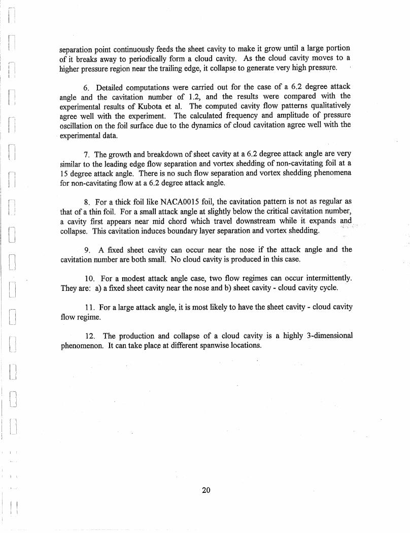
separation point continuously feeds the sheet cavity to make it grow until a large portion of it breaks away to periodically form a cloud cavity. As the cloud cavity moves to a higher pressure region near the trailing edge, it collapse to generate very high pressure.

6. Detailed computations were carried out for the case of a 6.2 degree attack angle and the cavitation number of 1.2, and the results were compared with the experimental results of Kubota et al. The computed cavity flow patterns qualitatively agree well with the experiment. The calculated frequency and amplitude of pressure oscillation on the foil surface due to the dynamics of cloud cavitation agree well with the

. experimental data.

7. The growth and breakdown of sheet cavity at a 6.2 degree attack angle are very similar to the leading edge flow separation and vortex shedding of non-cavitating foil at a 15 degree attack angle. There is no such flow separation and vortex shedding phenomena for non-cavitating flow at a 6.2 degree attack angle.

8. For a thick foil like NACA0015 foil, the cavitation pattern is not as regular as that of a thin foil. For a small attack angle at slightly below the critical cavitation number, a cavity first appears near mid chord which travel downstream while it expands and collapse. This cavitation induces boundary layer separation and vortex shedding.

9. A fixed sheet cavity can occur near the nose if the attack angle and the cavitation number are both small. No cloud cavity is produced in this case.

10. For a modest attack angle case, two flow regimes can occur intermittently. They are: a) a fixed sheet cavity near the nose and b) sheet cavity .. cloud cavity cycle.

11. For a large attack angle, it is most likely to have the sheet cavity - cloud cavity flow regime.

12. The production and collapse of a cloud cavity is a highly 3-dimensional phenomenon. It can take plac~ at different spanwise locations.

20

REFERENCES

Acharya, M., and Metwally, M. H., 1992, "Unsteady pressure field and 'Vorticity production over a pitching airfoil," AIM Journal, 30: 403-11.

Carr, L., 1988, "Progress in analysis and prediction of dynamic stall, II Journal of Aircraft, 25: 6-:-17.

Chandrasekhara, M:S., Carr, L. W., Wilder,M. C., 1'993, "Interferometric investigations of compressible dynamic stall over a transiently pitching airfoil," AIM Paper 93-0211.

Currier, J., and Fung, F.-Y., 1992, "Analysis of the onset of dynamic stall," AIM Journal, 30: 2469.-77.

Doligalski, T. L., Smith,C. R, and Walker, J. D. A., 1994, "Vortex interactions with walls," Annu. Rev. FluidMech., Vol. 26,pp. 573-616.

Fox, R W., and Kline, S. J., 1962, "Flow regime data and design methods for curved subsonic diffuser," Journal of Basic Engineering, Trans. ASME, Vol. 84, pp. 303-312. .

He, J. and Song, C.C.S., 1991, "Numerical Simulation and Visualization of Two­dimension.a1 Diffuser Flow", ASME, FED-Vol. 128,355-361.

Helmholtz, H., 1868, liOn Discontinuous Movements of Fluid" Phil. Mag., 36, No.4, 337-346.

lzumida, Y., Tamiya, S., and Kato, H., 1980, liThe relationship between characteristics of partial cavitation and flow separation," Proc. 10th IAHR. Symp., Tokyo, pp. 168-181.

Kawanami, Y., Kato, H., Yamaguchi, H., Tagaya, Y., and Tanimura, M., 1996, "Mechanism and Control of Cloud Cavitation," FED-Vol. 236, pp. 329-336.

Kirchhoff, G., 1869, "Zur Theorie Freier Flussigkeitsstrahlen", Jr. reine u. angew, Math., 70, 289-298.

Kiya, M." and Sasaki, K., 1985, "Structure of large-scale vortices and unsteady reverse flow in the reattaching zone of a turbulent separation bubble, II Journal of Fluid Mechanics, Vol. 154, pp. 463-491.

Kubota, A., Kato, H., Yamaguchi, H., and Maeda, M., 1989, "Unsteady structure measurement of cloud cavitation on a foil section using conditional sampling technique," Journal of Fluids Engineering, Trans. AS:ME, Vol. 111, pp. 204-210.

21

I'

Ii I:

1 I l

'I I : l!

n u

lJ o [J

[]

[]

U l-1 J

I :

i I

Kubota, A., Kato, H. and Yamaguchi, H., 1992, "A new Modeling of Cavitating Flows: a Numerical Study of Unsteady Cavitation on a Hydrofoil Section", Journal of Fluid Mechanics, Vol. 240,59-96.

MacCormack, R. W., 1969, "The effect of Viscosity in Hypervelocity Impact Cratering", AIAA Paper 69-354, Cincinnati, Ohio.

McCroskey, W. J., 1982, "Unsteady airfoils," Annu. Rev. FluidMech., vol. 26, pp. 285 ... 311.

Riabouchinsky, D., 1919, "On Steady Fluid Motion with Free Surface", Proc. London Math. Soc. 19,206-215.

Smagorinsky, J., 1963, "General Circulation Experiments with the Primitive Equations," Monthly Weather ReView, Vol. 91, No.3, pp. 99-164.

Song, C. S., 1965, "Two-dimensional Supercavitating Plate Oscillating Under a Free Surface", Journal of Ship Research, Vol. 9, No.1, 40-55.

Song, C.C.S. and Yuan, M., 1988, "A weakly Compressible Flow Model and Rapid Convergence Methods", Journal of Fluid Engineering, Vol. 110, 441-445.

Song, C. C. S., 1996, "Compressibility boundary Layer Theory and its Significanceiu·,. Computational Hydrodynamics", Journal of Hydrodynamics, Series B, Vol.. 8," . No. 2, 92-101

Song, C.C.S. and Chen, x., 1996, IICompressibility Boundary Layer and Computation of Small Mach Number Flows", Hydrodynamics, Theory and Applications, Proc. 2nd International Conf. on Hydrodynamics, Hong Kong, 815-820.

Tulin, M. P., 1958, "New Development in the Theory of Supercavitating Flows ll , Proc. Second Symp. on Naval Hydrodynamics, ONRIACR-38, pp. 235-260.

Wu, T. Y., 1956, "A Free Streamline Theory for Two-dimensional Fully Cavitated Hydrofoils II , Journal of Mathematics and PhYSics, 35, 236-265.

Yuan, M., 1988, "Weakly Compressible Flow Model and Simulations of Vortex-Shedding Flow about a Circular Cylinder," Ph.D. Thesis, University of Minnesota.

Zaman, K. B. M. Q., McKinzie, D. J., and Rumsey, C. L., 1989, "A natural low­frequency oscillation of the flow over an airfoil near stalling conditions, II Journal of Fluid Mechanics, Vol. 202, pp. 403-442.

22

[]

n r·~1

I I I ! l J

n I I , I

)1 ~ I

lJ

I I

i I

r 1

Figures 4-1 through 6-23

23

Ii : .1 I

II lJ 11 \ I LJ

I I I '

Fig. 4-1 Medium mesh system (381x64x3) around a NACAOO15 foil.

24

a. U

I

t-..) VI

3.0

2.5

2.0

1.5

1.0

0.5

0 . .0

, -0.5

i-- -- 1---;

\ \ \

r----. , , ,, _____ J :~

~ ..

\

Attack=O.O Oeg, Computed - - - - Attack=4.0 Oeg, Computed

\ , '\

\ ,. - - - Attack=8.0 Oeg, Computed

• Attack=O.O Oe9, Experiment

,......... I '- ' I ...... • ......

• Attack=8.0 Oeg, Experiment ... Attack=4.0 Oec, Exoeriment

\. ...... -...... ...... ...... ..... ........

..... - "­..... - ............. -- ........ .. _ ...... - ...... - ...... . ... ...........

._,--... ------ --:.1::-, --~- --, --- ----- --::-, --------- -, -... :--------:' ... ----, -- --- --f " --- .,.-f /' --=--~-

1/ --~ , I '/

-1.0 0.0 0.1 0.2 0.3 0.4 0.5

xlc 0.6 .0.7 .0.8 .0.9

Fig. 4-2 Comparison of computed pressure coefficients with experiment data (Izumida, et aI., 1980) for NACAOO15 foil at non-cavitating condition.

1.0

I' I i t .1

I, I !. i I

n I i

,-'I

I I ; J

r--, j I

II

-1

\.1 , I

I I

r I I

C. () I

3.5

3.0 G-----e Coarse mesh (191 x32x3) G-----e Medium mesh (381 x64x3)

2.5 ~ Fine mesh (761x128x3)

2.0

1.5

1.0

0.5

0.0

-0.5

-1.0 0.0 0.1 0.2 0.3 0.4 0.5

xlc

Fig. 4-3 Computed pressure coefficient distributions along foil surface based on three different mesh systems: coarse mesh (191x32x3), medium mesh (381x64x3), and fine mesh (761x128x3).

26

1.0

,

,- \ . i I

! 'l r

r ' I \ )

1 1 !,

r~-\

i \

I: J

:1 \ --

r- \ [_ J

1---',

1.J

\-1 I \ '- -

I \ lJ

\ I

c:::: (a)

c:::: (b) ~~ 0

• Q OC c:::: - --~~Q.Oo

(c)

c::::: - =--(d)

Fig. 4-4 Instantaneous vorticity component (roz) contours on the mid-span cross-section of NACA662-415 foil at a=6° during one period of trailing edge vortex shedding.

27

,-'

I

I,

11 , I

\]

L_i

Position 1

Position 5

Position 4 o o

Velocity (u) Frequency Analysis by FFT, Attack=6 degrees

1 .0 --,--------,----------------,

o l-

0.8

t) 0.6 Q) 0..

(J)

I­Q)

~ 0.4 0....

0.2

Legend at lead suction side * at middle suction side 0

at trail suction side x

at wake close to frail 0

a t xl c = 1 . 5 ,y I c = O. 1 5 b-

Lift !8l

Position 1

Position 2

Position 3

Position 4

Position 5

o.o~~~~~~~~~~~~~~~

0.0 0.4 0.8 1 .2 St. Number

1 .6 2.0

Fig. 4-5 Velocity (u) spectra at 5 positions and the lift spectra Jor NACA662-415 foil at a=6°.

28

,-I I I I , ,

r-, ; \

I

r-l, ! I i , i J

I~ I !, \. I

,--, I I I ! i I

'--1 I I LJ

i !

i I

) I

. (a)

•

-o "'00 ••

(

Fig, 4--6 Instantaneous vorticity component ((J)z) contours on the mid-span cross~section ofNACA662-415 foil at a=10·,

29

il \. l

n

1\

Ll·

C\ , I , ,

, I I

I ,,~

1 I i I

Fig, 4-7 Close-up of the leading edge vortex shedding during one cycle.

featured by instantaneous vorticity component (Wz ) contours on the mid-span cross-section ofNACA6~-415 foil at a=10·,

30

1~1

I I , i

-'~\

I I,

I

I ,

J i

; -\ r \

L._..I

Position 1

Position 5

Position 4 o

o

Velocity (u) Frequency Analysis by FFT, Attack= 10 degrees

16.0~--------~--------------~--~~

14.0

12.0

o ~ 10.0 (j (J) 0..

(f) 8.0 I­(J)

~

oc: 6.0

4.0

2.0

Position 1

Legend at lead suction side * at middle suction side 0

at trail suction side x at wake close to trail 0

at x/c= 1 .5,y/c=0.15 6-

Lift 181

Position 2

Position 3

Position 4

Position 5

0.0 -l-J~~!:"""':~~~~~ ....................... ~....-­, 0.0 0.2 0.4 0.6

St. Number 0.8 1.0

Fig. 4-8 Velocity (u) spectra at 5 positions and the lift spectra for NACA662-415 foil at a=10°.

31

[-'I I,

\ I

'~1

11 (

I 11 I I

. i I , ' l,,,1

o I

o·

J ..

o O~O ='

Fig. 4-9 Instantaneous vorticity component ( lOz) contours on the mid-span cross-section ofNACA66241S foil at a=lS" during one period of stall washout.

32

I

! \

I , r

Position 1

Position 5

Position 4 o

o

Velocity (u) Frequency Analysis by FFT, Attack= 15 degrees

24.0 ...-,----------,-------------, Legend

20.0

o 16.0 !.-

-+-' U ill 0...

(f) 12.0 !.­OJ ~ o

D- 8.0

4.0

at lead suction side * at middle suction side 0

at trail suction 'side x

at wake close to trail 0

at x/c= 1 .5,y/c=0.15 I.:.

Lift 181

Position 1

. Position 3

Position 4

0.0 -+-~-,-:~--,-:~~.~~ ..... ~ .... ~~ 0.0 0.2 0.4 0.6

St. Number 0.8 1.0

Fig. 4-10 Velocity (u) spectra at 5 positions and the lift spectra for NACA66r415 foil at a=15°.

33

'I ! '( I ,

j

r'

n \_1

r,-1

LJ

\] I II

U

................ ". ........ .-.............. ,.,.. ...... -- ..... ".---- .. .:- .................... -.. ". .. ". .... - ...... , .... ........ flO .............. __ ......... ". -........ "'"

:;1": ......... --.-....... #" ..... :- ... ,~'", ........ ... ::! -, " ... , .. ~"~",~', ... : ........................ ~ "' .. '" ... ~\~~,,~'\\ ..................... .. '.. \ \ ... ... . ',,: ...... : ................ .

',410" ..... IiIt .......... .

... 4io : .......................... ..

.. .. .. .. .. .. .. .. .. .. .. .. .. ..

.. ...... .{{(((((((((( - -: -::::: ~::: : : . .. : : : : :.:: : ~ ~ : ~ ~ ~ ~ ~ ~ ~ ~ ~ ~ ~ ~

.. ....... -. . .... 111!--- .. -... -."'--- ... _-- ... . _- ......... _---_ .. .......... .. .. ...... "!" fII".,.

.... -.................. .,. ..... , .... -...... ---......... .................... .. .. .. .. .. ... .. .. .. ~,,",: ........... " .. .. .. .. • .' • • • .. '" .. - .... .... .... fill .. ".f.F/. - •• ,., ............... , ::1/6 ....... "~.:: ......... : ........ \'\, .... "'.. . .... "", ,. ........................... ..

•• ',' ' ................. IIt ....... .. :'." , ...... II :~"" ...... _ ....... . ..... . . .:.' ..... ""' ...... . .. .... . ........................ ..

.. ::~!~~} ~ ~\".:::.}:.:::::::?:: .. : : : : : : : : .. .. : { { { { { {({ ({ { ( - ............... :.: ... :::: .. ::::: .. ::::::::::::~; ................................ _ .....

.. '!II ........ : ............ - ...... ______ _ ..... -.-._------_ .. _ .. --..............•.

Fig. 4-11 Instantaneous ,velocity vectors on the mid-span cross-section of NACA662-415 foil at a=15°.

34

rl , I l :

, J

rl i 'I ; I I ,

\~l I "

.)

,­,

, I,

! i I _

,

I 'I \

Cl'

o· 00 -D

(Q)G ?

o

. , . •

/)

Fig. 4-12 Instantaneous vorticity component (lOz) contours on the mid­span cross-section ofNACA662-415 foil at a=20°.

35

I

iJ

~I

I :

I / \ .

l ;

,I I 'I I )

i I u

pi U

Position 1

Position 5

Position 4 o o

Velocity (u) Frequency Analysis by FFT, Attack:=20 degrees

16.0~--------~--------------------~ Legend

14.0

12.0

o ~ 10.0 u ill 0..

(J) 8.0 l..... ill ~

~ 6.0

4.0

2.0

at lead suction side * at middle suction side 0

at trail suction side x at wake close to trail 0

at x/c= 1 .5,y/c=0.15 6.

Lift 181

Position 1

o . 0 -+---.----,r---T""~...,....-:;....---,---.--..,.......:~~:=;:!!2~~~~::bI

. 0.0 0.2 0.4 0.6 St. Number

0.8 1 .0

Fig. 4-13 Velocity eu) spectra at 5 positions and the lift spectra for NACA662-415 foil at a=20°.

36

[I I I I ' I I

\\

I-I U

L\

\\ .

( I L\

~J

I \

(J

Fig. 5-1 Jnstantaneous vorticity component ( CO,) contours on the mid-span cross-section of an E.N. foil at a 0=6.2" under non-cavitating condition.

37

I I I I I I I I I I I I I I I I I I I I I I I . I I I I I I I I I I I I I I I I I I I I I I I I I I I I I I I I I I I I I I I I I I I I I I I I I I I I I I I I I I I

( I

\ \

1\ \ '\

\

[\

\\ \ \ U

\\

II,

-----

----------------

----~I""'I

------------- -- ------~----------------- ----- ----- ----

= = = - --= --- -- -- -- ---- ------

~-- -:::----- --:: --- -- -- --===;= ;=----:::::::

'. -:: --- - -- - - - .: : : - - - - : : -- - =- =- = = : : : : : : : : -

------ ----------: ---:: :: :: :: :: ------ - ---- -: : : : : : : : :

--- ---- -----::---- -- ------ --::------- -----

---- ---- : -- ---- -- --- -= = :: : : - - -- -- -- -- --- - --- -: : : - - - -: : : : : :

- - ----.:-- - - --: -- - - - .: .: .:.: .: ::.: :: -- -- -: -: -= -= -:: - :: -= -: : :::: :: -------------------------------:_-::::::: ::.::::::: = -- --- -- -:: -:-: ::::: ~~::: ~~~ ~:::::----- - - -- - --- - --- - -.: :: : - -------- ----- -------: : : : --

Fig. 5-2 Time-aVeraged velocity field around an E.N. foU at a=6.2" undet non-cavitating condition.

38

I I I I I I I I I I I I I I I I I I I I I I I I I I I I I I I I I I I I I I I I I I I I I I I I I I I I I I I I I I I I I I I I I I I I I I I I I I I I I I I I I I I I I I

I ~i

Ci f I I I , )

r-; , , i.1

r~1 I

[l 11 iJ

U '~1 l_

1-' . I lJ

[J

,/

./

/ / / I I .-

/ .-/ / /

,/ ", ".

/' ,/ -.,/ . ".. ".- ..... /' - "-,/ ,. -...

Fig. 5~3 Close~up ofthe velocity field at the leading edge of an E.N. foil at a=6.2° under nOi1~cavitating condition.

39

n i 1

11 \ I

11

i[j

,- I

LJ

I i

I j I

Fig, 54 Time-averaged pressure coefficient contours around an E.N. foil at a:::;6.2D under non-cavitating condition.

40

r-1 I I I ,

il : -\ I I

I I

i J

r-j L~

'-I ! I LJ

(-I

l I

fi

IJ

U

SHEET AND CLOUD CAVITATION SIMULATION Mean Pressure Coefficient (Cp) on Foil Surface (EN Foil), CI=O,754

4.0 Legend

3.5 Non-Cavity Flow,Attack=6.2 *

3.0

2.5

2.0 0..

0 I

1.5

1.0

0.5

0.0

-0.5

-1.0 , 0.0 0.2 0.4 0.6 0.8 1 .0

X/c

Fig. 5-5 Time-averaged pressure coefficient distribution along E.N. foil surface at a=6.2° under non-cavitating condition.

, 41

..j:>.. tv

'------_____ -.J ~~" r--'--

\~ __ -.-J ~-) --I

-~

Unsteady Cloud Cavitation (E.N. Foil, a = 6.2 0 ,(1 = 1.2)

o

~.", (a)~ObU

o ....

-::::::::--" • 0 <> _ .~ (b)~ ~ GlOO Q ;;.

~ ~~? °D ( ) - -~

C? 0<::) ~

°0 .....

Computation (vorticity)

Fig. 5-6 Instantaneous vorticity component (OJ z) contours on the mid-span cross-section of an E.N. foil at a=6.2° under cavitating condition of <T=1.2.

Experiment (photographs)"

." , Fig. 5-7 Experimental photographs taken by Kubota et al. (1989) for an E.N. foil at a=6.2° under cavitating condition of <J=1.2.

~ w

L __ "-,--, r---' C~ ;- i

~ ==] .-----1

Velocity Field Comparison (E.N. Foil, a = 6.2 0 ,CJ' = 1.2)

(a) Computation

• - 0 ~r:-y l.. I"r-'Y .~ .-.. ~

: '. 1.0 I/e •

I·'r--, ·-l ... ~

: ,'i . i .... ~--.:... ~'~ : ~ ~ ~ ~~'~ ~~ \ ~--;;;::::::..-,;.' '\ ~' ~ -~H ' ,

h' : : ,. ~::..

:-

l.l •••• 0 ~ ~'l I.'f ~ ··1... '- • ·i .. , Y

. . , ' , , ,,-...... 1

.. ,1- \\ ~_ ...... ' • A

~ ... . . ,

: ~ &, .... , . ..) ~ " -... "

" . .

. . , . .. ....,.,.... , . : ~,l" \' '. • , 'I • J

~~J , .

(b) Experiment

1.,[ ......... .. ~ .L-'" .

.. _. " . . " (~-'\' :, ' .. -- . ~:.

:-- '

~-I.' •. r •

. : : i[)-;-... .".",. ' .... 11 .. ,

.;--; ... ' - (... I

~:

Fig. 5-8 Comparison of computed velocity field with experimental result (Kubota et al., 1989) of flow over an E.N. foil at a=6.2° under cavitating condition of 0'= 1. 2.

_J __ 0"1

____ ---.J

I I I I I I I I I I I I I I I I I I I I I I I I I I I I I I I I I I I I I I I I I I I I I I I I I I I I I I I I I I I I I I I

\

\ I

J

--------------------------- ------~--- ... -- -~----

,-

!

= :: ::-

= :: = -----=--- -

-~-------::::: -- -- -- --

-- ------- ------ --------- ----- ---. ------- ----: ----:: - -:::::-------- - -:: -- - -:: :: ---- --- ------

--- ------ --- --- ---- -------'-- ------ ----::::::-------:-----::::-----

--- ---- ----------:----- -------------- ------ - .. ---------~----:::---- -:::---------._- --- --- --- ----

Fig.5-9 lnstantanWUS velocity field around an E.N. foil at a=6.Z" under cavitating condition of (1= 1.2.

44

'1 II

n u

n \]

II U

u n u

lJ n U ,'---1 I I U

I '

,- , 45

[]

n l j

Cl L J

o

il LJ

\ \

I '. I

y

(a) x/c=O.25

(b) x/c=O.65

• I

(c) x/c=1.0S

+ +

t

Fig. 5~11 Computed time-space (t,y) distributions of vorticity component

(lOz) at three vertical sections: (a) xlc=O.25; (b) xlc=O.6S, (c) x/c=1.05, for an E.N. foil at a=6.2° under cavitating condition of CT= 1.2.

46

n [1'

[1

[I ("1

II . I L,'

~l \ I LJ

'~1

I ! U r-l

IU

I,U I i I

I '

, !

Y/C Y(M! VORTICITY (III)

80 70

0,4 ~O

$0 40

0.2 30

o

20 10 o

Fig. 5~12 Measured time~space (t,y) distributions of vorticity component (li)~) at xlc=1.05 (Kubota et aI., 1989) for an E.N. foii at ,cx=6.2° under cavitating condition of (1:1.2.

47

n n ~\

[I

Cl ,I

[l

\-11 L

IOJ

r--. \ LJ

!l \....,

'-, , U r--I LJ ~-l

U r--) l.J C-)

I j u

fl U

I [j

I

, i I

I J ,

~~ 0,11() .

0.40 .

=~ 0.0 ;!D.O 40.0 II().O 1I().01oo.0 120.0

lU~ m M . & 0.4 J ~== ..0.20•0 ;!D.O 40.0 . II().O II().O 100.0 120.0

-~ 0.11()

0.40 =~ ~.200.0 ;!D.O 40.0 80.0 80.0 100.0 120.0 11mI (l1li) .

. ,(a) Computation

X/C-O.85

X/C-O.65

X/C-O.45

Fig. 5-13 Comparison of computed pressure with experimental data· (Kubota et al., 1989) at three locations on foil surface for an E.N. foil at a=6.2° under cavitating condition of 0"=1.2.

48

fl

"', I \ I j

I 'i

III

\]

'1 !I I,J

c

i U I ,I

1.0

0.0 X/o=1.05

-1·~.00

x/o=0.85

0.0 x/o=0.45

x/o=0.25 -1 . 0 Lt-...J.....'---'--L..'---'-...J.....J......J..--1-L-L...--1-L--L.-L...L-L...-L-'--'-...!-J"::-:-~'---'----'-:-:-::"---1-L.-I.....-J

~.OO 0.05 0.10 0.15 0.20 Time (8)

Fig. 5-14 Computed long period pressure change with time at five locations on foil surface for an E.N. foil at a=6.2° under cavitating condition of (j= 1.2.

49

1', 1 I \1

ii' , 1 I,

[1

o U r-) L}

u

i I

" I

S'

0.'

O.!! •

0.2

o

~ 0.30 ~

~ 0.20

a; E 0.10 o z

o 0.1 0.2 0.3

Experiment

0.00 0 0.00 0.05 0.10 0.15 .20

Time (8)

Computation

Fig. 5 .. 15 Comparison of computed normal velocity at X/c=1.25 and y/c=0.133 with experimental data (Kubota et al., 1989) for an E.N. foil at a=6.2° under cavitating condition of (J'= 1.2.

so

0.. u I

I \ . U

SHEET AND CLOUD CAVITATION SIMULATION Mean Pressure Coefficient (Cp) on E.N. Foil Surface, Attack=6.2 degrees

4.0 ----rr----------,-------------,

3.5

3.0

2.5

2.0

1.5

1 .0

0.5

0.0

-0.5

-1.0

.0.0 0.2

Legend Non-Cavity Flow ?IE

Cavitation No.=0.7 0

Cavitation No.=1.0 x Cavitation No.= 1.2 0

0.4 0.6 0.8 X/C

1.0

Fig. 5-16 Computed time-averaged pressure distributions on E.N. foil surface at a=6.2° with different cavitation numbers.

51

r ~

i I I, ~

r-: I '

I i:

lJ

Ii I !.

[--I I I \~

[1

U [I LJ

I I

L.

1.0

0.9 -,,--,

c <::l.. 0.8 --<::l.. '-'

"1-1

~ 0.7 -

..... ~ 0.6 I-~ ~

<:> 0.5 U I-

~ 0.4 .r;j I-

~ ~ 0.3 I-

0.2 .....

0.1 .....

0.0 0.00

I I I I I I I I I

r -

-

-

-

-

-

J -

I I I I I I I

0.01 0.02 0.03 0.04 0.05 0.06 0.07 0.08 0.09 0.10 Pressure Coefficient

Fig. 6-1 Relationship between pressure and density

52

o o D

r I

Li I I I

I i I

(a) High speed photograph of cavitating flow taken by Kubota et al. (1992).

(b) Computed instantaneous density distribution

Fig. 6-2 Comparison of vortex-type cavity appearance on NACAOO15 foil at a=20· under' cavitating condition of a=1.7, (a) experimental photograph; (b) computed density distribution.

53

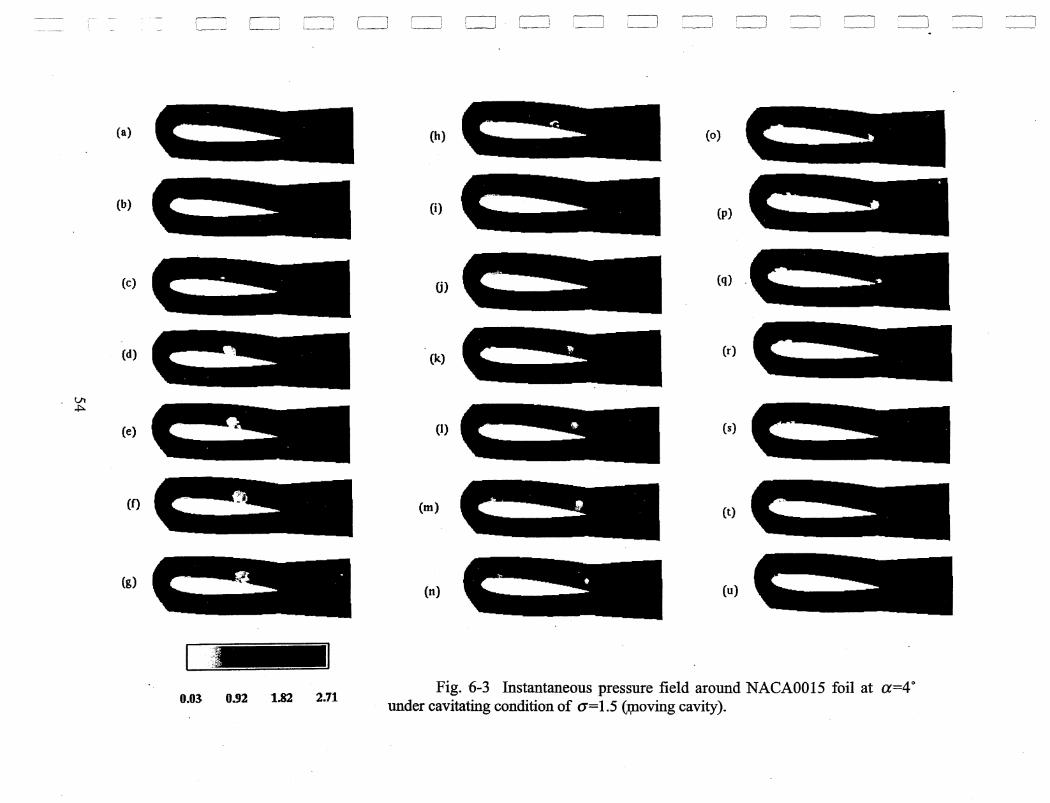
Vl ..j::>.

(a)

(b)

(e)

(d)

(e)

(f)

(g)

I ~ c=J i l CJ c::::J CJ CJ CJ -'--1 ~ __ I r:=J 1 ~l CJ ~

~ __ i . )

O.Ol 032 1.82 2.71

(h) (0)

(i) (p)

(j) (q) .

(k) (r)

(I) (s)

em) (t)

(n) (a)

Fig. 6-3 Instantaneous pressure field around NACA0015 foil at a=4° under cavitating condition of 0-=1.5 (tpoving cavity).

==:J ---r

VI VI

(a)

(b)

(e)

(d)

(e)

(f)

(g)

i i C-'i r-' L.----J ! 1 c=J c=J

(h)

(i)

(j)

(k)

(1)

(m)

(n)

c::::J c::J I j L_J ,----, ~

(0)

(P)

(q)

(r)

(s)

(t)

(u)

==:J

Fig. 6-4 Instantaneous density distributioll around NACA0015 foil at a=4° under cavitating condition of cr=1.5 (moving cavity).

,---, ~ ----"J :----,

~ ~ ------1

r----

VI 0'1

(a)

(b)

(e)

, (d)

(e)

(f)

(g)

l~ '-i r-, L----J '--------'

~-.

-16.0 -0.7 14.7 30.0

'--'I I~

I~ ,.--, ~, ~ I~~_.J L-...-J c:=J ~ L-=:J :~ =:J , I ==-:J

(h) (0) ~".

(i) (p) ~-.,.

(j) ~~- (q) _-.'-"" . (k)

(I)

(m)

(n)

~­~-.

~--.

~---

~'.-"

(r)

(5)

(t)

(u)

~ -~

....~ ..........

" ' .. .. '" ,

l

Fig. 6-5 Instantaneous vorticity around NACA0015 foil at a=4° under cavitating condition of a= 1.5 (moving cavity) . ..

=:J

Vt -..J

(a)

(b)

(c)

(d)

(e)

(I)

0.82

r--, c-: r-\ I i '------'1 I ] I~i j'---"l '~--.J I L....-...----.J. L--.........J ~ ~

~."" •... ;i

_C' .. '" .'"

4 • ,· ... c., ,-":

(g)

"""'.

~~ (h)

~ (1)

~., 0)

{:tc,

~ .. (k)

~, (I)

'C,,_ ..

~ •• "l'<:;,~i" ' .. ' . . ,"',,' '-"-......

..... ' .• " ,"_",.,..c.-, ' __

~"."""'" ~~

. ';";i:~:.~ .~

~"'. ~

~" .... "' •.. ;:~.j:.... :off!!'

'. ,'" ..

~wf: ~ ..

-~ , ~....J L~ • I

(m)

(n)

(0)

(P)

(q)

(r)

~ c==J :-i.l~

..... " ... :'"'''.. • .' . • J .•

, .~-, "",:~ ,': ,,~.

........

.. "" .. < ..•. :{,,?:"~2.!;:i~ ..t' " .. ',' I

'" .. I

. '

~ ....................... :t ..... '<' .. . ~ .. ~

~,

~& ~

~.~

.1.39 2.76 Fig. 6-6 Instantaneous pressure field around NACA0015 foil at a=4 D

under cavitating condition of CT=1.0 (stable sheet cavity).

Vl 00

(a)

(b)

(c)

(d)

(e)

(f)

,~--,

L~~ Ii L l r-] c=J c=:J . r--) :-l --~

,-----, L-..J L_ -\ ~~

~~.--J ~; 1 --~!

(g) (m)

(h) .. -_ .... ~~ (n)

(1) (0)

0) (P)

(k) (q)

(I) (r)

Fig. 6-7 Instantaneous density distribution around NACA0015 foil at a=4° under cavitating condition of (1=1.0 (stable sheet. cavity).

~

~

~-

~.

'-~ c--, '----------J

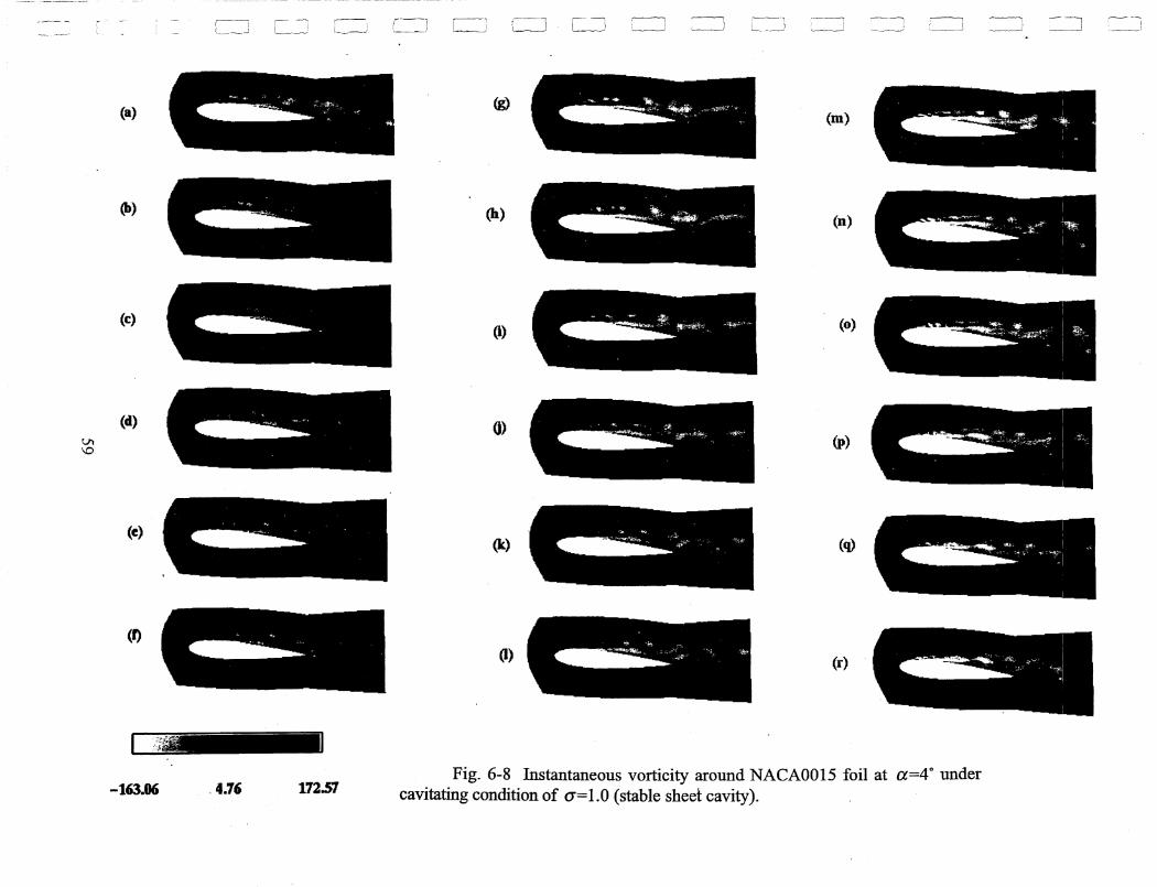
Vl \0

!-

(a)

(b)

(c)

(d)

(e)

(f)

-163.06

------ ---~ --~ -- ---

~i Lc- i r-- i r-----; '-1 ,--, l __ ..J --.J L~ __ ,--! l-...-.) L.--.J c=J(J'~ L _-.-J

c;-Z'1 -;-,;t~,-, (g) ~. ~;: ~

-?t

(h) .. ~-~

(1) :{,.~\ ''!'f;~~lif' _ ......

0) ~;p";,;;,,

(It) c_v .... ,"J;:,,"'. ,.~;..'

(I) -"'"' ~~,. ~A~

:~

(m)

(n)

(0)

(P)

(q)

(r)

-'I ;----' ------' ~ ~

, -]

--iI>-

~. '~~

~~;$."'~'

~-"~'- . :,:.:.:_~~'~"'-C-!

~

~""

.4.76 172.57 Fig. 6-8 Instantaneous vorticity around NACA0015 foil at a=4" under

cavitating condition of u=1.0 (stable shed cavity).

~, -I . __ .1

0"1 o

(a)

(b)

(e)

(d)

(e)

(f)

c---

L~' ,

L __ ~ '~~}

,,~ ,t ,l;j~" , J ~~F~'

~:{~:,. - ~ .'i""- I}

.~~

~.~~"H

~it~ !~~

~,~

0.02 0.85 1.67 2.50

,----~.

(g)

(h)

(i)

OJ

(k)

(I)

~ ~-__ J

~4'~~

~~

.... , 1'1,.~,!r> Ff ",;.i!,~~. ;.xt~"f .... _.,-

~"f~

~ ~.~

~ '~~

0'-1.0 SHEET CAVITATION

, "'"-.----------'

(m)

(n)

(0)

(p)

(q)

(r)

PRESSURE(ATTACK ANGLE=8 DEG. NACA0015)

--, I

~ '*"~

~~ ~~C"'l:'."" .~. "",,"">.. ,- '-l~f t"" ... '., .'~ .. -*

.e}~

~ J~

f­~~.

Fig. 6-9 Instantaneous pressure field around NACA0015 foil at a=8Q

under cavitating condition of (j=l.O (stable sheet cavity). '

-~I ~_.....o

-- ::J ----I

,.-------J

0\ .....

(a)

(b)

(e)

(d)

(e)

(f)

L-~ c_......------'

~';I"~

~-:!.

~~

~ .~

L_~j

. (g)

(h)

(i)

0)

(k)

(\)

.-~' , '. l--=-~!

,~ \

''--------~

-.........&

a-l.O SHEET CAVITATION ,

(m)

(n)

(0)

(p)

(q)

(r)

DENSITY(ATTACK ANGLE=8 DEG, NACA0015)

,----'

Fig. 6-10 Instantaneous density distribution aroupd NACA0015 foil at a=S' under cavitating condition of (1=1.0 (stable sheet cavity).

=J ===

0\ N

(a)

(b)

(e)

(d)

(e)

(f)

,--i_~~·

J -l '--~_.----/

,--" )-~I L..-.-.J ,'---------'

~.~~.<-;~2._~~~~;,;~1'::-~-;":'~Jf ,t_~~~~~r;_'~, ~" ')C.',*,~' •. .t'''.:f'w\.jt~. -,~~ ~'(;'

- ",....qp

~~.jft~f~~:f~~~~.

~;1~~tfF

~~;iJi~t~~'

~~1l~;'¥<£:4~'

~-

-16.V -'.7 14.7 ~.O

r-J

(g)

(h)

(I)

(j)

(k.)

(I)

a-LO

r----i ~

~1 [---, (--'1

L_l ~ ~

~;~"~~

~.,';·ttt4t,r·' -- '4

~:.r

~:~:,

~:.:.v.

SHEET CAVITATION

!'--\ .-----'

(m)

(n)

(0)

(p)

(q)

(r)

=-~ __ J ~--- -"I

'-~.----c=J

; -; ~;<'f~-}~~~l~~l:i ~~'~"J.t'·Mj "-i:~ ~~!. "':-

~:~~:lr.

'~~'~J~:~:t "c{ ... : ~ ..

,------, ,--j

~4-~>;.~f~.

~~;~~b:c~ft.w! ~~'

~~~~;l.f:~>~~""7 ~,<'"

VORTICITY(ATTACK ANGLE=8 DEG. NACA0015)

Fig. 6-11 Instantaneous vorticity around NACA0015 foil at a=8' under cavitating condition of (1=1.0 (stable sheet cavity).

-, . __ -..1 :~:=-l

0\ W

(a)

(b)

(e)

(d)

(e)

(f)

~--'~

@J' .. < :,:'ir~_; '-~~~Ai:~ ~~"~ ~;!,;;~'·il~" ..... ~~~ ~,- .. "",,:". -F~:- -~ '-'~ ~

" /", .', ' \,

~",,: '~"i:':~~_Jiij -"'. ';;.~~ "" . h. "'" .. ~_~~;-: :>t,~\. .... --.

~'. , .. ~;?;§~,-- '.}"'-: ~

~~''l.'''C'''''' "~';'!",'; • ';''1. ~ :?K'. 5"'4; _'" -~< . ~~~li~~~_~~'4:~.

"'~~';';:;~'t r ~".,~,':, ;"'<f ,'. "f>J,', ~

. '" ',',t:t.:';;.lt;,;:''11:; .' :

0.02 0.&5 1.67 2.50

C~ --~i ,r--l

L-~-~-----..--' ~~

(g)

(h)

(i)

(j)

(k)

(\)

, n;lilt:·~ ~ ~~l ;~ ~),t

{ ~,~, :·r,;.~~,,::.~~.. p

, "t·l~d • \Il~ , • ~:.'~'f 1 " ~:-.:-" '~-?'~~~ .. ~,:~~?~~::~ .. ~

~-. ~t·. _-r;';;- :":~""'~:\.ft... "1

~,1~~~' fl,' ~.l~::~' ': ':\",,~")'"

..±1t':~.:~1i.~~ " ~'~"

. '''' . J.1~ ""i "'Ja);,j ~'~~":-i4l';~'l,~' ~\~~" ~ri!~

rr-1.0 CLOUD CAVITATION

--1 , --!

(m)

(n)

(0) c:_ (p)

(q) ~~'," ~ ;-/~, , ", ",~:-

...... ' "

(r) S

- .• h~ ff' ,.. ~v, -f ...". 1i.-l' ~4f.a~1I,,;"" ;', A,' ~. 'lit -'_~~~~v. ~~ ,~' . PRESSURE(ATTACKANGLE=8 DEG, NACA0015)

Fig. 6-12 Instantaneous pressure field around NACA0015 foil at a=8° under cavitating condition of 0'=1.0 (sheet and cloud cavities).

~[ ~.--. "~I

<.-....--~.---'

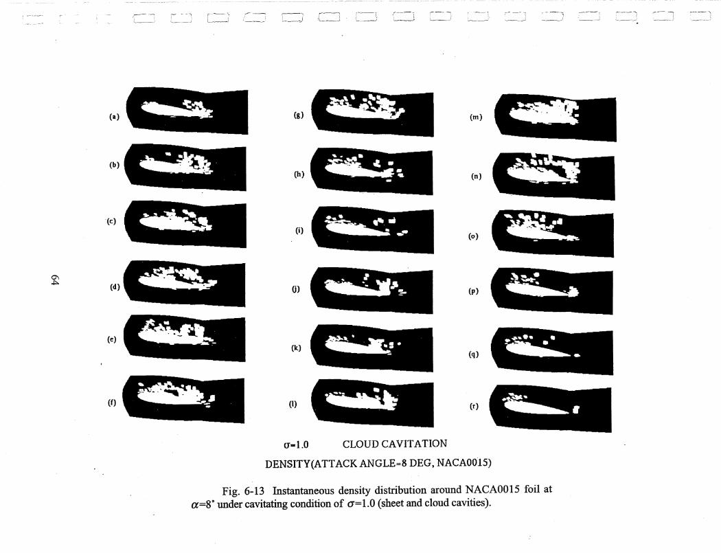
0\ ~

(a)

(b)

(e)

(d)

(e)

(f)

'~---..

'---------' ,--, L.-----J ~'_, __ J .~.---=:\ L--..-J

(g)

(h)

(i)

0>

(It)

~'# • ,,-. . .. -~ .... " -.,-

I ~.: ... ~ ~~

~.

.----,

(m)

(n)

(0) -= (p)

...... ...... (q)

.,....... . ~ . ..

~~ (1) ~ (r) ~.

u-1.0 CLOUD CAVITATION

DENSITY(ATTACKANGLE=8 DEG, NACA0015)

Fig. 6-13 Instantaneous density distribution around NACA0015 foil at a=So under cavitating condition of <1=1.0 (sheet and cloud cavities).

"--1 --1

0\ Vl

-,,--'-"~ =J __ --1 ---' r--- -

;......._."_--:;;;.J

'--I ,~--'

(a)

(b)

(e)

(d)

(e)

(f)

~';~~ 'I'

.. ' ,., .. ;, ~~ft..,~~4,~.\~~;;;;.,~; ~::'::::;¥i.,.lJ'.~ ~-.- . .,

~~~~'f

~~~t~{

~~~~

~·">,:.?'~ii;:;"~~:~fJ~~~~11;; ~~'~",~ ~-:-,--\ ..

-16.0 -0.7 14.7 30.0

(g) ~~r~.~i.~~~~~

(m)

(h) ~:f~:;=~~'~~i (n)

(i) ~!:~~~:f~: (0)

(j) ~;,\;!~{:~;t!~)t

(p)

(k) ~~:;:'~:~i~~C

~- ~ -~ ",., (q)

(1) ~t~~~:~: (r)

a-l.O CLOUD CAVITATION VORTICITY(ATTACKANGLE=8 DEG. NACA0015)

_~:..,~;,7(';;·1!:.·~:'~'~k. ·.'?~i~.ir : ~~(-$~' ~-~~"-.~ ~>-

',>.< !-t 'C" K"~', " '. ,_". ~ . ~ "~l :~ ~~ -~~. i1h tf; i'~ ~4~tw~;~r: -,,~~. "'~""~'1:"'P;~~;-'~-~ .~'p" ~.~ .--.-- .~ ... --~. -

~ ~~~~~.~~,,,

~ ~

,-:~ .. , ... ":,,, .. , '. . '. "4~:~ __ '-';~'4.~~."', ·f?: _";"~' ... ,.~. _.:.;~~ . < '" :Co-, .::\.. _ .,; _ '~> ~'''"''~~.;:~.'''.''''<. <, ' .. . ", "-. '...".

- ---:--- - ",.

Fig. 6-14 Instantaneous vorticity around NACA0015 foil at a=8° under cavitating condition of a=1.0 (sheet and cloud cavities). '

---- i

0\ 0\

(a)

(b)

(e)

(d)

(e)

(l)

0.02

- , I \-=J

~~.~--~

, ! '-------.-...:;.';c-"

'.1 __ II i ;

L--J ----1

._---....:::-l

(g)

(h)

(i)

(j)

(It) (q)

(r) (I)

IT-1.0

0.85 1.67 250 PRESSURE(ATTACKANGLE=20 DE,G. NACA0015)

Fig. 6-15 Instantaneous pressure field around NACA0015 foil at a=20· under cavitating condition of 0'=1.0 (sheet and cloud cavities).

,~-l

-_.;...--.-J _ __ J --

0\ 'I

(a)

(b)

(e)

(d)

(e)

(f)

:' ~~- ~---- , ~ _~~J

- r-i ,--~,

,...--- i· _' __ 0)"

r----' I \ ~'

--, ,-----~~ j L_ _ ~~_>'

(i)

(j)

(k) (q)

(I) (r)

(1-1.0

DENSITY(ATTACKANGLE=20 DEG, NACA0015)

Fig. 6-16 Instantaneous density distribution arou:p.d NACA0015 foil at a=20' under cavitating condition of (}=1.0 (sheet and cloud cavities).

- ---~\

---~ ~~~-::J ;~~_J

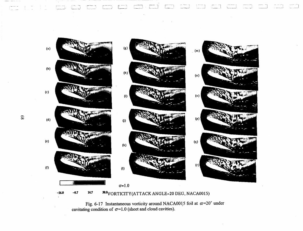
0\ 00

(a)

(b)

(e)

(d)

(e)

(f)

1--

-16.0

c_~ C=' L=J L ___ :J 1-~1 L ... ____ ; ~~.---J ~~~-J !

(g)

(h)

(i)

(j)

(k) (q)

(I) (r)

(f-l.O -0.7 14.7 3O·OyORTICITY(ATTACKANGLE=20 DEG. NACA0015)

Fig. 6-17 Instantaneous vorticity around NACAOOl,5 foil at a=20· under cavitating condition of cr=l.O (sheet and cloud cavities).

--=-=1 _~.--J ~ -- --1 -~:.

\

il

Iii

I I I . . I

II l

P II

u

Section 1 (NZ=2)

Section 2 (NZ=15)

Section 3 (NZ=28)

5.93

3.96

1.99

0.02 0"=1.0 t{f=16.72

PRESSURE FIELD (ATTACKANGLE=8 DEG. NACA0015. NS. NZ=29)

Fig. 6-18 Instantaneous pressure field around NACAOOI5 foil at three span-wise sections at a=8° under cavitating condition of 0"=1.0. (a) left end section (Section I. NZ=2) , (b) mid-section (Section 2, NZ=I5), (c) right end section (Section 3, NZ=28).

69

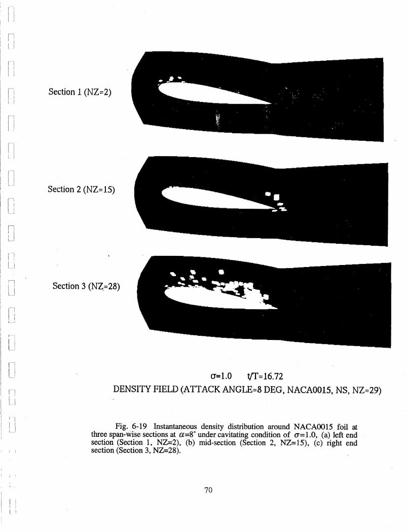
n [I

rl I j

Ii Section 1 (NZ;::2) , I II

il I II

1--' , I

I' ____ ---.J

1', : .. j. l_

Section 2 (NZ= 15)

n Section 3 (NZ,=28) lJ

,-, I ' Li

ri I I l_1

i I

I '

a=1.0 t{f=16.72

DENSITY FIELD (ATTACK ANGLE=8 DEG. NACA0015, NS, NZ=29)

Fig. 6-19 Instantaneous density distribution around NACAOO15 foil at three span-wise sections at a=8° under cavitating condition of (1=1.0, (a) left end section (Section 1, NZ=2), (b) mid-section (Section 2, NZ=15), (c) right end section (Section 3, NZ=28).

70

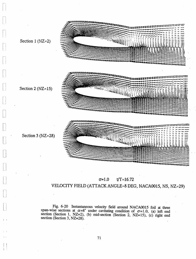
r\, lJ

II n

o o D o o o u o o i i

; \

\ \

Section. 1 (NZ=2)

Section 3 (NZ=28)

0'=1.0 t{f=16.72 VELOCITY FIELD (ATTACKANGLE=8 DEG. NACA001S. NS, NZ=29)

Fig. 6~20 Instantaneous velocity field around NACAOO15 foil at three span~wise sections at a=8° under cavitating condition of 0'=1.0, (a) left end section (Section 1, NZ=2) , (b) mid~section (Section 2, NZ=15). (c) right end section (Section 3, NZ=28).

71

[I

[1

Ii [l [-.-1

_,

Section 1 (NY =1, Surface)

Section 2 (NY =9)

[1 Section 3 (NY = 15)

U

L1

[]

[j

U I I I

5.93

3~96

1.99

0.02 0"=1.0 t{f=16.72

PRESSURE FIELD (ATTACKANGLE=8 DEG, NACA0015, NS, NZ=29)

Fig. 6-21 Instantaneous pressure field around NACAOO15 foil at three vertical levels at a=8° under cavitating condition of 0"=1.0, (a) foil surface level (Section I, NY=1), (b) y/c=0.05 (Section 2, NY=9), (c) y/c=0.1 (Section 3, NY=15).

72

r­il

, [-1, I I I

Il I I

[1

[J

[I

(]

! U

lJ,

U

I I

Section 1 (NY:::l, Suriace)

Section 2 (NY =9)

Section 3 (NY = 15)

a=1.0 t{f=16.72

DENSITY FIELD (ATTACKANGLE=8 DEG, NACA0015, NS, NZ=29)

Fig. 6-22 Instantaneous density distribution around NACAOO15 foil at three vertica1levels at a=8° under cavitating condition of 0'=1.0, (a) foil surface level (Section 1, NY=1), (b) y/c=0.05 (Section 2, NY=9), (c) y/c=0.1 (Section 3, NY=15).

73

, I

rl I I I (

I' • I I I I

rl

II

n il

[\ ["1 lJ

[\ '"1 I I u

Section 1 (NY:::1, Surface)

I"P

Section 2 (NY::: 9)

--Section 3 (NY::: 15)

I' I

r ,.tl I -

------"'~ .. , .". .. #",.,._,..,"~ ~"" ,,., _ ..... ". ". ". ",. "'" _ ...... ___ -"t _ - ....

,."" ,I,..,.". ~ ,. , I """ f# f' ~ •• I , , {I .. ,. .. .,. .... _ ~ ~ ~ ~ - ......... - - - - ---...... ". '-!I"~~ I' ~" II f # •• " " t , ,., f" .. ~ __ --~ -- .... - - .... _ ...... - - ----•• , ... I I • .,..".,,~ ~" , .... , , , ",. ....... " ... '" __ .- ~;# ~ .. _ ~ .... ____ ...... __

__ ~"'.'f! ..... ,.' f".""." .. II ....... --""..- ... .,..., .. _ ....... .,....-_,..._

.·-'.~ .. ··".IiI~ .. ~' ...... ".~. I'" .. _,.,..~",.~,,- ____ -.._~_

.... :;:.::.: ... :.':::::;.::;;;~'. ~~~: ::.::'::====.:::===:::::.:::. . , ... , ... ,,, .. ,.,,, ... ,,,,, .. , .~-_.,.I;-_------- ........... ~ .... • , ..... , ~, ... I"f"-"~ """''''''' •• ', .. _"'~"'-~""If"'#_-.,---"" ___ ~-.. ..... -..~ I I" ...... , , ......... _ ... ,.".". " f" _ " I , ,. ,.,...". - .- .". _ ..... -.......---,. ~ _ -... __ ...... --. .'I."' ............ __ .. "~IIfI_,. .. ""'." " ... __ "...".fII" __ .....--.----..... __ ---.-.. ..... ~

:.~:~~:::: :~~::=::::~::~,~,::: ::::::;::':;':::::=:::--':::'==::::::== '" ••• ~ .. , " ... II , • , • " • ~ , ••• "'\ ,," , , , • .. ~ _~_ ........ """'- ,"- _______ ..... __ -","'.""''''''''' ....... ,.",."~,,., 'I"'" I, " .. # _~,._ ... ~,;::::::. __ """ _ .... -..

:~:::~:~~~~:::':-~~~::: ~:~:::: ~ ~; ~! ;:::.::::~::.::::=:::~::::::: .~'/~." •••• ~# •••• , • •• ~ ....... ,. .. - ... ---- ..... --. ........... " .... -

oq~"'I!"".'."~"'-"~'" •• "'", ..... ", .. ,. ~""'" ..... ____ -. __ ........... ....., ....... ~-~ • y-rd4o"''' .". """.'" '" !II .. _ •• , • " ..... ~ ~ .... _ .. _______ ........... -.. ......... _ ............ _---

... ~~ •• ,'~ •• ""''''''' ,,,iII~lo ••• ,., •• .,. ...... __ ~~-______ ~ "'J',~ ... ,. ....... ,",,,,,,,,,,'"'''''''''''' ~ .... _ ... _ ...................... _____ _

........ :::!:~::~:~~::::~~:::::::~ : ~ ~ :::.~~ ~ = :::::-===::-::-=:: ===::a= , ..... " • , , f , ... ,. f#'" • '\ , ___ ". , , • .. ....... _ f"" _____ ~ ... ~ .. _ - ". fI" """' ... , .......... " ..... -- .. ,.., ... __ .. __ ....... '"' .......... - _ .. ~

----"" ............. 10"' ... ----------... "" "''' .. ,,,, .. ,,, ...... -------------"\'~ "' ..... , .. .,."\ -"""""..,.,.. '" -----------"---....... ~--""''''----~ .. ~.".-''''''. ~ -- .... ---~-,.--~-1 !",! .. _~_ .. ".".,.~" .. " ~ _____ - _______ _ .. , .... .,.,,-_. .., ",,- ",~~---------~-

~I/J"",_""_"",,,,~-_,,, ......... ", "., ~ ".,..."". ________ ...... .."... ........ ".'''.,'' .... f .. _~"""'"",,,,..... _________ ...

• • •• ,. •••••• ., t1': II , , I I ,. _ "." """ ~ ___ ..... ,.... __ .--__ --.....~ - - , " • 1 • I • , •• , .. _ ,. \ • , , '" ___ ~.",-..".,...-'.--_______ --.... .....

""_"""_.~"."" .. '. I, """''''''~''''''''''''~''''-~ _____ -. ....... .... ,. .. ~ .. "'f" .,.. f ~,. -~~ .... ,-----------... .......... - ____ -... "' .... ".", •••• "" 1iII""" __ """""""~"""'''-____ ,"",",''''''----'''' __ ........ , 1 •• 1 •• '" ••• ~ .... _ ~ ",. """,,~ _ """ _ - - _ ..... --.",- __

... "'t#f.~ ............. , .. "- ... ,.,. .... """'~_. __ """"' ___ ....... , __ __

... ;;.~;.::.:::::;::.::~=-:.:.:.:.::.==::.::=..:.:.:::::::: =~:::==::: =-;::::~ ~ ~::::::~:::::::.: :==:::-----:::.::..=..:::::::. =. = ::: ::

-~,."-.,-",.",,,."'----- _--...--,--. - ..... -.. ~:.:::::::: ::-;~ ;:~~~~ .. ~ :-:::::::.-~=====:::::::::::::::::.::. = ,,."" .. _ ...... ~,." .... , 0""'" ... "" .... ________ ""-" ..................... ""'-"\ .... _

.... " •• ,,"' ••.• , .... , .'tI~_ .. ____ .. __ ... __ """--..... - - ........... '""_ ~ • " .' • ~ • " - ... '" .... - ... 'lito ... --. -... ........ - -

(1'=1.0 t/T=16.72 VELOCITY FIELD (ATTACKANGLE=8 DEG, NACA0015, NS, NZ=29)

Fig. (j~23 Instantaneous velocity field around NACAOO15 foil at three vertical levels at a=8° under cavitating condition of 0"=1.0, (a) foil surface level (Section 1, NY=1), (b) y!c=0.05 (Section 2, NY=9), (c) y/c=0.1 (Section 3, NY=15).

74