kyei barfour.pdf
74
59 KWAME NKRUMAH UNIVERSITY OF SCIENCE AND TECHNOLOGY INSTITUTE OF DISTANCE LEARNING TOPIC: MODELLING QUEUING SYSTEM IN THE BANKING INDUSTRY: CASE STUDY GHANA COMMERCIAL BANK, SUAME, KUMASI ECOBANK, ASHTOWN, KUMASI AND BARCLAYS BANK OF GHANA, TANOSO BRANCHES By KYEI BAFFOUR, YAW ANOKYE, BSc MATHS A Thesis Submitted To the Department of Mathematics, Kwame Nkrumah University of Science and Technology In partial fulfilment of the requirement for the degree of MASTER OF SCIENCE Department of Mathematics Institute of Distance Learning
-
Upload
doankhuong -
Category
Documents
-
view
220 -
download
3
Transcript of kyei barfour.pdf

59
KWAME NKRUMAH UNIVERSITY OF SCIENCE AND
TECHNOLOGY
INSTITUTE OF DISTANCE LEARNING
TOPIC:
MODELLING QUEUING SYSTEM IN THE BANKING
INDUSTRY: CASE STUDY
GHANA COMMERCIAL BANK, SUAME, KUMASI
ECOBANK, ASHTOWN, KUMASI AND
BARCLAYS BANK OF GHANA, TANOSO BRANCHES
By
KYEI BAFFOUR, YAW ANOKYE, BSc MATHS
A Thesis Submitted To the Department of Mathematics,
Kwame Nkrumah University of Science and Technology
In partial fulfilment of the requirement for the degree of
MASTER OF SCIENCE Department of Mathematics
Institute of Distance Learning

60
DECLARATION
I hereby declare that this submission is my own work towards the MSc. and that, to the
best of my knowledge, it contains no material previously published by another person nor
material which has been accepted for the award of any other degree of the University,
except where due acknowledgment has been made in the text.
……………………... ………………….…… …………………
Kyei Baffour, Yaw Anokye Signature Date
(PG 2011508)
Certified by:
Prof. S. K. Amponsah Signature Date
(Supervisor)
Certified by:
……………………. ………………….…… ………………………….
Prof I. K Dontwi Signature Date

61
DEDICATION
This work is dedicated to my wife, Dorcas; daughter, Nhyira; parents, Very Rev & Mrs Kyei
Baffour, and all my siblings, teachers and all those who contribute to the betterment of the
well being of humankind.

62
ABSTRACT
The issue of queuing is a bother to both management and customers in the
delivery of service in the banking industry. The main idea or pivot of the queuing system is
a teller who provides some services to a population of customers. This study therefore
determined whether the present capacity level in the banking industry strike a balance
between waiting and service time using Barclays Bank, Tanoso Branch, Ghana Commercial
Bank, Suame Branch and Ecobank, Ashtown Branch as a case of interest. Primary data on
five hundred and fifty-eight (558) customers arriving at the case of study throughout the
selected hours and days were collected, taken into consideration; the arrival, processing
and departure times of each customer. By using the queuing rule First-come, First-serve as
practiced by the case study and 𝑀𝑀/𝑀𝑀/𝑠𝑠 queuing model, the performance measures were
calculated uncovering the applicability and extent of usage of queuing models in achieving
customer satisfaction at lowest cost by minimizing waiting times, idle times, capacity
utilization and queues at the bank. The study shows how the data collected at the
respective dates possesses the Markovian properties, that is, Poisson and Exponential
Distributions, hence the use of two “M’s” in the 𝑀𝑀/𝑀𝑀/𝑠𝑠 queuing model. It determined the
probabilistic analysis that the teller(s) is idle and also determined the probability of certain
number of arrivals occurring at a given time. It was observed that any time the number of
tellers at BBG an Ecobank were reduced to two during a peak day, the queue elongated
resulting in high capacity utilization factor and hence a high waiting time. It is therefore
recommended that management makes better decisions relating to number of tellers that
would be necessary to serve customers during peak and off-peak hours, days and weeks.

63
TABLE OF CONTENTS
CONTENT PAGE
NUMBER
DECLARATION I
DEDICATION ii
ABSTRACT iii
TABLE OF CONTENT Iv
LIST OF TABLES vii
LIST OF FIGURES viii
LIST OF ABBREVIATION x
ACKNOWLEDGEMENT xi
CHAPTER 1
INTRODUCTION
1.0 Background of the Study 1
1.1 Statement of the Problem 4
1.2 Objectives of the Study 8
1.3 Methodology 9
1.4 Justification 9
1.5 Limitation 9

64
1.6 Organization of the Thesis 10
CHAPTER 2
LITERATURE REVIEW
2.0 Introduction 11
2.1 Evolution of Queuing Theory 11
2.2 Queuing Researches In The Banking Industry 18
CHAPTER 3
METHODOLOGY OF THE STUDY
3.0 Introduction 21
3.1 Primary Data Collection 21
3.2 Description of Queuing System 22
3.2.1 Queuing Systems in the Banking Industry 24
3.3 Fundamental Queuing Relations 26
3.4 Customer Arrival and Inter Arrival Distributions 26
3.4.1 Probability Distribution 27
3.4.2 Exponential Distribution 27
3.4.3 Poisson Distribution 28
3.5 Teller Utilization Factor (𝜌𝜌) 30
3.6 Little’s Law 30
3.7 Queuing Model Description 31
3.7.1 𝑀𝑀/𝑀𝑀/1 Model 32

65
3.7.2 𝑀𝑀/𝑀𝑀/𝑠𝑠 Model 35
3.8 Data Sheet Processing 39
CHAPTER 4
ANALYSIS AND DISCUSSION OF RESULTS
4.0 Introduction 40
4.1 Primary Data Examination 41
4.2 Discussion Of Findings 44
4.3 Queuing Model Analysis 48
4.3.1 Performance Analysis 49
CHAPTER 5
SUMMARY, RECOMMENDATIONS AND CONCLUSION
5.0 Introduction 54
5.1 Summary of Findings 54
5.2 Conclusion 55
5.3 Recommendation to Stakeholders 56
5.4 Recommendation to Future Researchers 57
BIBLIOGRAPHY 59
APPENDICES

66
Appendix 1.0 64
Appendix 2.0 68
Appendix 3.0 73
Appendix 4.0 75

67
LIST OF TABLES
TABLE
NO. TITLE
PAGE
NO.
4.1 Summary of Primary Data Collected on 27th, April, 30th April and
2nd May, 2012 43
4.2 Probability of the number of customers or fewer that would have
arrived using confident interval of 95%
46
4.3 Probability of the highest turning points of the Poisson Distribution
Graphs in Appendix 2.0
47
4.4 Probability that a customer and five customers are in the Queuing
system
50
4.5 Presentation of results for considering one to four tellers at a given
point in time
52
A1.0 Poisson Model for data collected on 30th April, 2012 66
A3.0 Queuing Analysis on data collected between 27th April, 2012 and
2nd May, 2012
74
68
LIST OF FIGURES
FIGURE
NO.
TITLE PAGE
NO.
3.1
3.2
Hypothetical structure of a Queuing system in banks
Single Tellers Queuing System
22
24
3.3 Multiple Tellers, Single-Stage Queuing System 25
3.4 Several ,Parallel Servers-Several Queues Model 25
3.5 Transition diagram for a single teller processing 32
3.6 Transition diagram for a multiple teller possessing 36
4.1 Graphical presentation of data collected at GCB on 2nd May, 2012 42
4.2 Poisson Arrival Distribution Graph for data collected on 27th April,
2012
47
4.4 Probability of a number of customers in the System for 27th April,
2012
51
A1.1 Graphical presentation of data collected at BBG on 27th April,
2012
64
A1.2 Graphical presentation of data collected at BBG on 30th April,
2012
64
A1.3 Graphical presentation of data collected at BBG on 2nd May, 2012 65

69
A1.4 Graphical presentation of data collected at Ecobank on 27th April,
2012
65
A1.5
Graphical presentation of data collected at Ecobank on 30th April,
2012
66
A1.6 Graphical presentation of data collected at Ecobank on 2nd May,
2012
66
A1.6 Graphical presentation of data collected at GCB on 27th April,
2012
67
A1.7 Graphical presentation of data collected at GCB on 30th April,
2012
67
A2.1 Poisson Arrival Distribution for data collected on 30th April, 2012 71
A2.1 Poisson Arrival Distribution for data collected on 2nd May, 2012 72
A3.1 Probability of a number of customers in the System for 30th April,
2012
73
A3.2 Probability of a number of customers in the System for 2nd May,
2012
73

70
LIST OF ABBREVIATIONS
ACRONYMS MEANING
GCB Ghana Commercial Bank
BBG Barclays Bank of Ghana
ECO Ecobank.
i.i.d Independent and identically distributed
r.v Random Variable

71
ACKNOWLEDGEMENT
It has been by the abundant grace and magnanimity of god that I have come this far. . I am
forever grateful to the omnipotent and ever loving God.
Special thanks go to Prof. S. K. Amponsah, my supervisor, whose resourceful knowledge
and guidance has helped me to come up with this thesis. Rev. Dr. William Obeng – Denteh
of the Mathematics department of K.N.US.T also deserve commendation for his
encouragement.
I wish to express my heartfelt thanks to the Branch Managers of Ghana Commercial Bank
(GCB), Suame Branch, Barclays Bank of Ghana (BBG) Tanaso Branch and Ecobank, Ashtown
Branch for given me the permission to use their respective outfit as the case of study.
Finally, to all my friends especially Emmanuel Oppong-Gyebi whose inputs into this work is
highly commendable, Richmond Asante, Isaac Adu Kuffour and all my relatives, it is through
your prayers, sacrifices and inspirations that have brought me to this level. I wish you God’s
abundant grace, love, peace, prosperity and guidance.
Kyei Baffour, Yaw Anokye.

72
CHAPTER 1
INTRODUCTION
1.1 BACKGROUND OF THE STUDY
The banking sector is the largest and most competitive segment of Ghana’s financial
sector. The liberalisation of the banking sector in the 90’s led to an increase in the
number of banks in the country. The universal banking concept introduced in 2003
by the Central Bank of Ghana also opened wide the doors of the Ghanaian banking
industry to investors who decided to establish as many as banks. Most of these banks
are operating in the country under African Ownership and management. Currently,
the number of banks operating in Ghana is 28 (BoG, 2010), with numerous emerging
and existing Rural Banks, Credit Unions and Micro Finance, but the aggressive
competition has forced long-operating banks to reconfigure their strategy and
business to sustain or improve their competitive advantage. Consequently, the
banking industries have largely implemented service delivery technology as a way of
augmenting the services traditionally provided by bank personnel.
Competition has become keener due to regulatory imperatives of universal banking,
technological inventions, quality of customers and globalisation of the market and
also due to customers’ awareness of their rights. Customers have become
increasingly demanding, as they require high quality, low priced and immediate
service delivery. They want additional improvement of value from their chosen
banks (Olaniyi, 2004). This has resulted in a paradigm shift in the banking business.
The modern banking in Ghana has shifted from a seller’s market to buyer’s market.

73
The buyer’s market puts emphasis on customer needs, wants and satisfaction.
Competition is making customer retention more important than ever. The bank that
is unable to satisfy its customers is likely to lose them. Actually, all banks suffer
from voluntary churn – the decision by the customer to switch to another bank. This
is particularly true for Ghanaian banks. Ankomah (2008) estimates annual churn rate
for banks to be between 10 and 18 per cent on average.
In this emerging market, customers are not that loyal to one particular bank and
managers are greatly aware that providing quality customer satisfaction is a key
retention component that results in the industry profitability. Hence, the major banks
have been forced to consider how to create a loyal customer base that will not be
eroded even in the face of fierce competition. Therefore, these banks must realize the
necessity of studying and understanding various antecedents (viz. service quality and
customer satisfaction) of the customer retention which might help them to develop a
loyal customer base. The banking industry, whose service depends on building long
term relationship need to concentrate on maintaining customer’s loyalty. In this
respect, retention is greatly influenced by service quality. As such, banks often invest
in managing their relationships with customers and maintaining quality to ensure that
customers whose loyalty is in the short term will continue to be loyal in the long
term, the need has also arise to bring sanity in the baking hall to avoid unnecessary
long queues. High quality service helps to generate customer satisfaction and
customer retention by soliciting new customers, and improved productivity and
financial performance.
As information technology becomes more sophisticated, banks in many parts of the
world are adopting a multiple-channel strategy. Changes in banking industry as a

74
result of challenges posed by technologically innovative competitors such as those
resulting from deregulation, rapid global networking, and the rise in personal wealth
have thus made the implementation of sophisticated delivery systems. The
technology of electronic banking, for examples; Automated Teller Machines (ATMs),
Internet, Mobile and Telephone Banking, etc, are aimed to render faster and
convenient banking services to customers in anywhere and at anytime, a strategy
necessary in many cases. These electronic banking has already advanced in the
developed countries, but only few customers in Ghana subscribe to it. However, it,
cannot entirely replace the more traditional channels. Research indicates that a
substantial portion of the customer base may always demand the type of personal
interaction that can only be provided by individual branch personnel (Lewis et al.,
1994). In other relation, it has been observed that, as the country population
increases, the customer population also increases. Hence, queue(s) may be witness in
the banking halls. At time, the subsidiary channel like, the ATMs do witness queues
by the customers, how much less queues at the respective banking halls in Ghana?
Since service delivery in banks is personal, customers are either served immediately
or join a queue if the system is busy. A queue occurs when facilities are limited and
cannot satisfy demand made against them at a particular period. However, most
customers are not comfortable with waiting or queuing (Olaniyi, 2004). The danger
of keeping customers in a queue is that their waiting time may amount to or could
become a cost to them (i.e. bank customers).
When we encounter a queue, we often make a quick estimate of the expected waiting
time and decide whether to join the queue based on the amount of time we are
willing to wait. Basically, queuing is a core of almost every transaction undertaken

75
by customers within banking industry. However, several concerns are being raised by
customers over the unsatisfactory service condition as a result of queue(s) delay.
There may be several factors arising to this fact, but not withstanding those
accessions, the ultimate aim for every customer is to spend limited time at the
banking halls. As a result of these constraints, most managers attempt to solve
queuing problems procuring additional facilities or hiring more workers to reduce
the waiting time.
Almost all banks are opening more branches and some are even forming mergers to
have a bigger capital base and also maximise profit. The most recent is Ecobank and
TTB in April, 2012 has increased their branches to forty-two (42).
1.2 PROBLEM STATEMENT
In this era of shrinking markets, banks can gain competitive edge over rivals by
devoting resources to improve customer satisfaction in order to retain existing
customers instead of wasting useful time and resource to win new customers.
Excellent customer satisfaction has a positive correlation with profitability, growth
and customer retention and on the other hand, poor customer service causes
considerable damage to goodwill of the banking industry and this eventually leads to
financial loss and dwindling market share. In this regards, customers must be
absolutely satisfied at the banking hall in order not to be stressed upon receiving and
paying in their own resources as a result of long queues, poor service quality and
unnecessary long waiting time.

76
Queue is a social phenomenon and if managed well, it would be beneficial to the
society, especially to both the unit that waits and the one that serves. Queue is a line
of customers waiting their turn for service. Queuing occurs when customers arrive
faster than they can be served and the system temporarily buffers them in queues.
Queuing system is a system that includes the customer population source, a queuing
discipline as well as the service system.
The ultimate objective of this analysis of queuing systems is to determine
whether customer satisfaction can be enhanced through managing the queuing
systems in the banking industry using selected cases of study so that informed and
intelligent decisions can be made in their management. This study is based on a
mathematical building process as well as designing and implementing of an
appropriate experiment involving that model. This encompasses the study of arrival,
behaviour of customers, service times, service discipline, service capacity and the
departure of customers at the case of interest, which is the marketing strategy of
many banks as well. The problems are categorised into three main parts and can be
identified as:
1. Arrival Problems. Usually, there is an assumption that service times are
independent and identically distributed, and that they are independent of the inter
arrival times. For example, the service times can be deterministic or exponentially
distributed. It can also occur that service times are dependent of the queue length.
Most queuing models assume that the inter arrival times are independent and have a
common distribution. In many practical situations customers arrive according to a
Poisson stream (i.e. exponential inter arrival times).

77
If the occurrence of arrivals and service delivery are strictly according to
schedule, a queue can be avoided. But in practice, this does not happen. In most
cases the arrivals are the product of external factors. Therefore, the best one can do is
to describe the input process in terms of random variables which can represent either
the number arriving during a time interval or the time interval between successive
arrivals. Customers may arrive one by one, or in batches. If customers arrive in
groups, their size can be a random variable as well. An example of batch arrivals is
the Customs Office at Aflao where travel documents of bus passengers have to be
checked.
Customer population can be considered as finite or infinite. When potential
new customers for the queuing system are affected by the number of customers
already in the system, the customer population is finite. When the number of
customers waiting in line does not significantly affect the rate at which the
population generates new customers, the customer population is considered infinite.
Banking customer population is infinite since they do not restrict a specific number
of customers to be serviced each day and work strictly with time.
2. Behavioural problems. The study of behavioural problems of queuing at
banks is intended to understand how customers behave under various conditions.
This normally affects the smooth service delivery irrespective of the facilities that a
bank may have if much attention is not given to it. Customer’s behaviour at the
banking hall may destruct attention of the one that serves and can bring serving to a
halt. A customer may balk, renege, or jockey and their queuing analysis is based on
behavioural problem researches. Balking occurs when the customer decides not to
enter the queue. Reneging occurs when the customer enters the queue but leaves

78
before being serviced. Jockeying occurs when a customer changes from one line to
another, hoping to reduce the waiting time. A good example of this is picking a line
at GCB, Suame Kumasi Branch and changing to another line with the hope of
serving quicker. The models used in this supplement assumed that customers are
patient; they do not balk, renege, or jockey; and the customers come from an infinite
population.
3. Operational problems. The operational system is characterized by the
number of queues, the number of tellers, the arrangement of the tellers, the arrival
and service patterns, and the service priority rules. Under this heading, all problems
that are inherent in the operation of queuing systems are included. How many
customers can wait at a time if a queuing system is a significant factor for
consideration? There may be a single teller or a group of tellers helping the
customers. If the banking hall is large, one can assume that for all practical purposes,
it is infinite. In many queues, it is useful to determine various waiting times and
queue sizes for particular components of the system in order to make judgments
about how the system should be run. Some of such problems are statistical in nature.
Others are related to the design, control, and the measurement of effectiveness of the
systems. In many situations customers in some classes get priority in service over
others. Also, there are other factors of customer behaviour such as balking, reneging,
and jockeying that require consideration as well. The slow pace and the number of
tellers also affect the time a customer waits in the queuing system.
1.3 OBJECTIVES OF THE STUDY

79
The primary objective of this study in line with the identified problems is to
determine whether the present capacity level in the banking industry, strikes a
balance between waiting and service time using Barclays Bank of Ghana, Tanoso
branch, Ecobank, Ashtown branch and Ghana Commercial Bank, Suame branch as
case study. This would be carried out by measuring customers;
a) The arrival time.
b) The processing time.
c) The departure time.
The study specifically aims to determine:
i) The probabilistic analysis that the teller(s) will be idle.
ii) The amount of waiting time a customer is likely to experience in a system;
iii) How the waiting time will be affected if there are changes in the facilities and
iv) Make policy recommendation base on the findings from the study.
1.4 METHODOLOGY
In an observational way, primary data would be collected at the same time and
date at the two cases of study in some selected days within January and February,
2010. Microsoft Office Excel 2007 would be used to assess and interpret data with
the help of various method of queuing analysis. Secondary data used to execute the

80
literature review of the study was gathered from the internet, professional magazines,
research papers, journals, and textbooks.
1.5 JUSTIFICATION
Queues are so commonplace in society that it is highly worthwhile to study them,
even if one waits in the check line for a few seconds. It may take some creative
thinking, but if there is any sort of scenario where time passes before a particular
event occurs, there is probably some way to develop it into a queuing model.
1.5 LIMITATION
It was a big task in observing and taking customers arrival, processing and
departure times, especially at GCB, Suame branch which use several single teller
with single stage queues arranged in parallel.
1.7 ORGANIZATION OF THE STUDY
Chapter one highlights on the background of study, the objectives, some of
the challenges faced during the study and the organisation of the study. Chapter two
shows the origin of queuing theory and also highlight on the works of some of its
contributors that lead to the study of this thesis topic. In chapter three, the
methodology used to achieve the objectives under study would be clearly stated.

81
Component of the basic queuing system, fundamental queuing relations and various
assumptions related to model development are explicitly mentioned, and overall
model structure would be explained. Analysis and interpretation of data collected
would be done in chapter four. Summary of findings, recommendation and
conclusion would also appear in chapter five.
CHAPTER 2
LITERATURE REVIEW
2.0 INTRODUCTION
This chapter shows the origin of queuing theory and also highlights on the
works of some of its contributors that lead to the study of this thesis topic.
2.1 EVOLUTION OF QUEUING THEORY
Queuing Theory had its beginning in the research work of a Danish engineer named
A. K. Erlang. In 1909 Erlang experimented with fluctuating demand in telephone
traffic. Eight years later he published a report addressing the delays in automatic
dialing equipment. At the end of World War II, Erlang’s early work was extended to
more general problems and to business applications of waiting lines.

82
In Erlang’s work, as well as the work done by others in the twenties and thirties, the
motivation has been the practical problem of congestion. Notable example is the
works of (Molina, 1927; Fry, 1928). During the next two decades several
theoreticians became interested in these problems and developed general models
which could be used in more complex situations. Some of the authors with important
contributions are Crommelin, Feller, Jensen, Khintchine, Kolmogorov, Palm, and
Pollaczek. A detailed account of the investigations made by these authors may be
found in books by (Syski, 1960; Saaty, 1961). Kolmogorov and Feller’s study of
purely discontinuous processes laid the foundation for the theory of Markov
processes as it developed in later years.
Noting the inadequacy of the equilibrium theory in many queue situations,
(Pollaczek, 1934) began investigations of the behaviour of the system during a finite
time interval. Since then and throughout his career, he did considerable work in the
analytical behavioural study of queuing systems, (Pollaczek, 1965). The trend
towards the analytical study of the basic stochastic processes of the system
continued, and queuing theory proved to be a fertile field for researchers who wanted
to do fundamental research on stochastic processes involving mathematical models.
To this day a large majority of queuing theory results used in practice are those
derived under the assumption of statistical equilibrium. Nevertheless, to understand
the underlying processes fully, a time dependent analysis is essential. But the
processes involved are not simple and for such an analysis sophisticated
mathematical procedures become necessary.
Queuing theory as an identifiable body of literature was essentially defined by the
foundational research of the 1950’s and 1960’s. The queue M/M/1 (Poisson arrival,

83
exponential service, single server) is one of the earliest systems to be analyzed. The
first of such solution was given by (Bailey, 1954) using generating functions for the
differential equations governing the underlying process, while Lederman and Reuter
(1956) used spectral theory in their solution. Laplace transforms were later used for
the same problem, and their use together with generating functions has been one of
the standard and popular procedures in the analysis of queuing systems ever since.
A probabilistic approach to the analysis was initiated by Kendall (1951, 1953) when
he demonstrated that imbedded Markov chains can be identified in the queue length
process in systems M/G/1 and GI/M/s. Lindley (1952) derived integral equations for
waiting time distributions defined at imbedded Markov points in the general queue
GI/G/1. These investigations led to the use of renewal theory in queuing systems
analysis in the 1960’s. Identification of the imbedded Markov chains also facilitated
the use of combinatorial methods by considering the queue length at Markov points
as a random walk.
Mathematical modelling is a process of approximation. A probabilistic model brings
it a little bit closer to reality; nevertheless it cannot completely represent the real
world phenomenon because of involved uncertainties. Therefore, it is a matter of
convenience where one can draw the line between the simplicity of the model and
the closeness of the representation. In the 1960’s several authors initiated studies on
the role of approximations in the analysis of queuing systems. Because of the need
for useable results in applications various types of approximations have appeared in
the literature (Bhat et al., 2002).
By the end of 1960’s most of the basic queuing systems that could be considered as
reasonable models of real world phenomena had been analyzed and the papers

84
coming out dealt with only minor variations of the systems without contributing
much to methodology. There were even statements made to the effect that queuing
theory was at the last stages of its life. But such predictions were made without
knowing what advances in the computer technology would mean to queuing theory.
At later instance, in the seventies, its application has been extended to computer
performance evaluation and manufacturing. The need to analyze traffic processes in
the rapidly growing computer and communication industry is the primary reason for
the resurgence of queuing theory after the 1960’s. Research on queuing networks by
(Jackson, 1957; Coffman and Deming, 1973; Kleinrock 1975) laid the foundation for
a vigorous growth of the subject. Some of the special queuing models of the 1950’s
and 1960’s have found broader applicability in the context of computer and
communication systems and some other real life problems such as banking,
manufacturing systems, to mention but a few.
In any theory of stochastic modelling statistical problems naturally arise in the
applications of the models. Identification of the appropriate model, estimation of
parameters from empirical data and drawing inferences regarding future operations
involve statistical procedures. These were recognized even in earlier investigations
in the studies by Erlang. The first theoretical treatment of the estimation problem was
given by (Clarke, 1957) who derived maximum likelihood estimates of arrival and
service rates in an M/M/1 queuing system. Billingsley’s (1961) treatment of
inference in Markov processes in general and Wolff’s (1965) derivation of likelihood
ratio tests and maximum likelihood estimates for queues that can be modelled by
birth and death processes are other significant advances that have occurred in this
area.

85
The first paper on estimating parameters in a non-Markovian system is by (Goyal
and Harris, 1972), who used the transition probabilities of the imbedded Markov
chain to set up the likelihood function. Since then significant progress has occurred
in adapting statistical procedures to various systems. For instance, (Basawa and
Prabhu, 1988) considered the problem of estimation of parameters in the queue
GI/G/1; (Rao, et al. 1984) used a sequential probability ratio technique for the
control of parameters in M/Ek/1 and Ek/M/1; and Armero (1994) used Bayesian
techniques for inference in Markovian queues, to identify only a few. More recent
investigations are by (Bhat and Basawa, 2002) who use queue length as well as
waiting time data in estimating parameters in queuing systems.
Hillier’s (1963) paper on economic models for industrial queue problems is, perhaps,
the first paper to introduce standard optimization techniques to queuing problems.
While Hillier considered an M/M/1 queue, (Heyman, 1968) derived an optimal
policy for turning the server on and off in an M/G/1 queue, depending on the state of
the system. Since then, operations researchers trained in mathematical optimization
techniques have explored their use in much greater complexity to a large number of
queuing systems. These have paved way for us to study the queuing systems in some
selected banks by using queuing theory.
Queuing Discipline, that is to say, when an arrival occurs, it is added to the end of
the queue and service is not performed on it until all of the arrivals that came before
it are served in the order they arrived. Although this is a very common method for
queues to be handled, it is far from the only way. Bank queues are typical example
that outlines a first-come-first-serve discipline, or an FCFS discipline. Barrer (1957)
compared this with a situation where the customers are served at random, and found

86
that the steady state probability of service is slightly less for random selection.
Another situation of interest has two classes of customer with different priorities.
Other possible disciplines include last-come-first-served or LCFS, and service in
random order, or SIRO. While the particular discipline chosen will likely greatly
affect waiting times for particular customers (nobody wants to arrive early at an
LCFS discipline), the discipline generally doesn’t affect important outcomes of the
queue itself, since arrivals are constantly receiving service regardless.
A probabilistic approach to the queuing capacity analysis was initiated by (Kendall,
1951, 1953) when he demonstrated that embedded Markov chains can be identified
in the queue length process in systems M/G/1 and GI/M/s. Lindley (1952) derived
integral equations for waiting time distributions defined at embedded Markov points
in the general queue GI/G/1.
Models with dependencies between inter arrival and service times have been studied
by several authors. Models with a linear dependence between the service time and
the preceding inter arrival time have been studied in (Cidon, et. al, 1991). Mitchell,
et al (1977) analyzes the M/M/1 queue where the service time and the preceding
inter arrival time have a bivariate exponential density with a positive correlation. The
linear and bivariate exponential cases are both contained in the correlated M/G/1
queue studied by (Borst,et al, 1993). The correlation structure considered in Borst,et
al (1993) arises in the following framework: customers arrive according to a Poisson
stream at some collection point, where after exponential time periods, they are
collected in a batch and transported to a service system.
Single-server queues with Markovian Arrival Processes (MAP), MAP/G/1 queue
provides a powerful framework to model dependences between successive inter

87
arrival times at the bank, but typically for the case where the arrival process is
Poisson and the service times are independent and identically distributed (i.i.d.)
random variables with a general distribution function G, has been investigated by
(Newel, 1966). The present study concerns single-server queues where the inter
arrival times and the service times depend on a common discrete time Markov
Chain; i.e., the so-called semi-Markov queues. As such, the model under
consideration is a generalization of the MAP/G/1 queue, by also allowing
dependencies between successive service times and between inter arrival times and
service times. The more challenging problem of customers’ behaviour on the waiting
time was first addressed by (Barrer 1957; Gnedenko and Kovalenko, 1968) in the
M/M/1 setting. There are also works on the similarly challenging problem of
customers’ behaviour on waiting plus service time, including (Loris-Teghem 1972;
Gavish and Schweitzer, 1977; Hokstad; 1979; Van Dijk, 1990).
In order to serve the customers at faster rates, there must be good customer advisors,
faster computers and better networks provided the computers are networked to avoid
queuing or jamming networks. The need to analyze service mechanism in the rapidly
growing computer and communication industry is the primary reason for the
strengthening of queuing theory after the 1960’s. Research on queuing networks and
books such as (Coffman and Deming, 1973; Kleinrock, 1976) laid the foundation for
a vigorous growth of the subject. In tracking this growth, one may cite the following
survey type articles from the journal Queuing Systems: (Coffman and Hoffri, 1986),
describing important computer devices and the queuing models used in analyzing
their performance.

88
Traffic processes in computers and computer networks have necessitated the
development of mathematical techniques to analyse them. The first article on
queuing networks is by (Jackson, 1957). Mathematical foundations for the analysis
of queuing networks are due to (Whittle, 1968; Kingman, 1969), who treated them in
the terminology of population processes. Complex queuing network problems have
been investigated extensively since the beginning of the 1970’s.
Customers finally leave one by one after being served. This is because each teller
can serve one person at a time. The interest of many researchers has not been in
customers’ departure, resulting in little or no research on departure.
2.2 QUEUING RESEARCHES IN THE BANKING INDUSTRY
Queuing-based teller staffing models was introduced into the financial industry in
the late 1960s and early 1970s primarily to control increasing labour expenses
(Brewton, 1989). Transactions such as deposits, withdrawals, and cash-checking
were handled exclusively by human tellers until the introduction of Automated
Teller Machines (ATMs). Although automated banking and on-line banking have
decreased the need for human tellers, many retail banks still rely on them to provide
timely and personalized customer service. Agboola and Salawa (2008) identified
various Information and Communication (ICT) in use and determined how they
could be utilized for optimal performance on business transactions in the banking
industry.
Price Waterhouse Cooper’s publication (1999) indicates that the primary aim of the
introduction of modern electronic delivery channels was to cut costs and congestions

89
by attracting lower-value customers to non-branch channels. However, the result was
quite different in the experimented areas from that expected: high-value customers
started to use these channels, while the lower-value customers continued to use
branches. This is never the same in a developing country like Ghana where every
customer want to correspond directly with the personal bankers.
Wenny and Whitney (2004) determined bank teller scheduling using simulation with
arrival rates. They investigated scheduling of banks at a branch in Indonesia and the
model accounts for real system behaviour including changing arrival rates, customer
balking and reneging for randomly selected hours in the day. Travis and Michael
(2007) assume that all servers at retail banking have the same service time
distribution and that this distribution is exponential. These assumptions are
motivated more by operational and analytical convenience than supported by data.
Oladapo (1988) study conducted in Nigeria revealed a positive correlation between
arrival rates of customers and bank’s service rates. He concluded that the potential
utilization of the banks service facility was 3.18% efficient and idle 68.2% of the
time. However, Ashley (2000) asserted that even if service system can provide
service at a faster rate than customer’s arrival rate, queues can still form if the arrival
and service processes are random. Emuoyibofarhe, et al., (2005) studied the queuing
problem of banks in Nigeria, taking First Bank plc, Marina branch Lagos as a case of
interest, and apply queuing theory to solve the multiple server problem (𝑀𝑀/𝑀𝑀/𝑠𝑠/./
∞/∞ queuing system) which yielded results upon which the management of the bank
could optimality distribute servers (cashier) to minimize waiting times, idle times
and queues in the bank.

90
One week survey conducted by Elegalam, (1978) revealed that 59.2% of the 390
persons making withdrawals from their accounts spent between 30 to 60 minutes
while 7% spent between 90 and 120 minutes. Baale (1996) while paraphrasing
Alamatu and Ariyo (1983) observed that the mean time spent was 53 minutes but
customers prefer to spend a maximum of 20 minutes. Their study revealed worse
service delays in urban centres (average of 64.32 minutes) compared to (average of
22.2 minutes) in rural areas. To buttress these observations, Juwah (1986) found out
that customers spend between 55.27 to 64.56 minutes making withdrawal from their
accounts.
Efforts in this study are directed towards application of queuing models in capacity
planning to reduce customer waiting time and total operating costs.
CHAPTER 3
METHODOLOGY OF THE STUDY
3.0 INTRODUCTION
In this chapter, the methodology used to achieve the objectives under study is
clearly stated. Component of the basic queuing system, fundamental queuing
relations and various assumptions related to model development are explicitly
mentioned, and overall model structure is explained.

91
3.1 PRIMARY DATA COLLECTION
Data was collected at an even time and date at the three cases of study. The
data of most fundamental importance were arrival time, service time and departure
time of customers. These data were randomly collected within an hour interval
between the period of 8:30am to 4:30 pm on 27th and 30th of April and 2nd May,
2012. These days are assumed to be some of the busiest days of the mouth. Summary
of the data collected are shown in Table 4.1 and 4.2. Monday and Fridays are
assumed to be the peak days for the case study, as customer’s business proceeds
from weekend are deposited in banks on Mondays and also the closing week’s
proceeds on Fridays. Most customers do withdraw for the weekends on Fridays.
Series of interviews and observations of customer’s attitude survey was also carried
out to know the causes of some customers reneging, balking or jockeying.
3.2 DESCRIPTION OF QUEUING SYSTEM
A queuing system can be described as customers arriving for service, waiting
for service if not immediate, utilizing the service, and leaving the system after being
served. Figure 3.1 shows the basic components of a queuing system and identify
them into four main elements namely: customer population, the queue, the service
mechanism and departure.
Service Mechanism Queue Calling
Population
Arrival point at the bank

92
Figure 3.1 Hypothetical structure of a Queuing system in banks
The queue discipline is the order or manner in which customers from the queue are
selected for service. There are a number of ways in which customers in the queue are
served. Some of these are:
Customers can be served one by one or in batches. In this context, the rules
such as;
i) Dynamic queue disciplines are based on the individual customer attributes in the
queue. Few of such disciplines are:
a) Service in Random Order (SIRO) - Under this rule customers are selected for
service at random, irrespective of their arrivals in the service system. In this
every customer in the queue is equally likely to be selected. The time of
arrival of the customers is, therefore, of no relevance in such a case.
b) Priority Service - Under this rule customers are grouped in priority classes on
the basis of some attributes such as service time or urgency or according to
some identifiable characteristic, and FCFS rule is used within each class to
provide service. Treatment of VIPs in preference to other patients in a
hospital is an example of priority service.
Service Process
Departure from the

93
ii) Static queue disciplines are based on the individual customer's status in the
queue. Few of such disciplines are:
a) If the customers are served in the order of their arrival, then this is known as
the first-come, first-served (FCFS) service discipline. Prepaid taxi queue at
airports where a taxi is engaged on a first-come, first-served basis is an
example of this discipline.
b) Last-come-first-served (LCFS) - Sometimes, the customers are serviced in
the reverse order of their entry so that the ones who join the last are served
first. For example, assume that letters to be typed, or order forms to be
processed accumulate in a pile, each new addition being put on the top of
them. The typist or the clerk might process these letters or orders by taking
each new task from top of the pile. Thus, a just arriving task would be the
next to be serviced provided that no fresh task arrives before it is picked up.
Similarly, the people who join an elevator last are the first ones to leave it.
For the queuing models, the assumption that customers are serviced on the first-
come-first-served basis would be considered.
The service mechanism can involve one or several queues consisting of more than
one teller arranged in series and / or parallel. But for these cases of study, the tellers
are arranged in parallel. The uncertainties involved in the queuing model’s service
mechanism are the number of tellers, the number of customers getting served at any
time, and the duration and mode of service. Random variables are used to represent
service times, and the number of tellers, when appropriate.
3.2.1 QUEUING SYSTEMS IN THE BANKING INDUSTRY

94
The central element of the system is a teller, who provides services to customers.
Customers from some population of customers arrive at the bank to be served. Some
of the services may include; cash deposit, cash withdrawal, cheque deposit and
withdrawal, foreign currency deposit and withdrawal, and enquires. Below are three
main queuing systems used in the banking industry:
1. Single Teller, Single Queue. The models that involve one queue – one service
facility are called single teller models where customer waits till the service
point is ready to take him for servicing.
2. Figure 3.2 Single Tellers Queuing System
3. Several (Parallel) Tellers, Single Queue – In this type of model there is more
than one teller and each teller provides the same type of facility. The
customers wait in a single queue until one of the service channels is ready to
take them in for servicing.
Arrivals Queue Service Facility Customers Leave
Arrivals Queue
Service Facility Customers Leave
95
Figure 3.3 Multiple Tellers, Single-Stage Queuing System
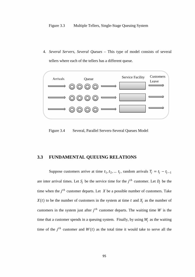
4. Several Servers, Several Queues – This type of model consists of several
tellers where each of the tellers has a different queue.
Figure 3.4 Several, Parallel Servers-Several Queues Model
3.3 FUNDAMENTAL QUEUING RELATIONS
Suppose customers arrive at time 𝑡𝑡1, 𝑡𝑡2, … 𝑡𝑡𝑗𝑗 , random arrivals 𝑇𝑇𝑗𝑗 = 𝑡𝑡𝑗𝑗 − 𝑡𝑡𝑗𝑗−1
are inter arrival times. Let 𝑆𝑆𝑗𝑗 be the service time for the 𝑗𝑗𝑡𝑡ℎ customer. Let 𝐷𝐷𝑗𝑗 be the
time when the 𝑗𝑗𝑡𝑡ℎ customer departs. Let 𝑋𝑋 be a possible number of customers. Take
𝑋𝑋(𝑡𝑡) to be the number of customers in the system at time 𝑡𝑡 and 𝑋𝑋𝑗𝑗 as the number of
customers in the system just after 𝑗𝑗𝑡𝑡ℎ customer departs. The waiting time 𝑊𝑊 is the
time that a customer spends in a queuing system. Finally, by using 𝑊𝑊𝑗𝑗 as the waiting
time of the 𝑗𝑗𝑡𝑡ℎ customer and 𝑊𝑊(𝑡𝑡) as the total time it would take to serve all the
Arrivals Queue Service Facility Customers Leave

96
customers in the waiting queue at time 𝑡𝑡 (the total remaining workload at time 𝑡𝑡), the
intermediate queuing relations such as Lambda (λ) and Mu (𝜇𝜇) are derived.
Lambda (λ) is the expected number of customers per whatever units 𝑡𝑡 is
measured in. 𝜆𝜆 = 𝑁𝑁𝑁𝑁𝑁𝑁𝑁𝑁𝑁𝑁𝑁𝑁 𝑜𝑜𝑜𝑜 𝑐𝑐𝑁𝑁𝑠𝑠𝑡𝑡𝑜𝑜𝑁𝑁𝑁𝑁𝑁𝑁𝑠𝑠𝑇𝑇𝑜𝑜𝑡𝑡𝑇𝑇𝑇𝑇 𝑡𝑡𝑡𝑡𝑁𝑁𝑁𝑁 𝐼𝐼𝐼𝐼𝐼𝐼𝑜𝑜𝑇𝑇𝐼𝐼𝑁𝑁𝐼𝐼
𝜆𝜆𝑡𝑡 is therefore the average number of customer arrivals during 𝑡𝑡 amount of time.
Mu (𝜇𝜇) is the average number of customers a teller can handle per unit time.
𝜇𝜇 = 𝑁𝑁𝑁𝑁𝑁𝑁𝑁𝑁𝑁𝑁𝑁𝑁 𝑜𝑜𝑜𝑜 𝑐𝑐𝑁𝑁𝑠𝑠𝑡𝑡𝑜𝑜𝑁𝑁𝑁𝑁𝑁𝑁𝑠𝑠 𝑇𝑇 𝑡𝑡𝑁𝑁𝑇𝑇𝑇𝑇𝑁𝑁𝑁𝑁 𝑐𝑐𝑇𝑇𝐼𝐼 ℎ𝑇𝑇𝐼𝐼𝐼𝐼𝑇𝑇𝑁𝑁𝑇𝑇𝑜𝑜𝑡𝑡𝑇𝑇𝑇𝑇 𝑡𝑡𝑡𝑡𝑁𝑁𝑁𝑁 𝐼𝐼𝐼𝐼𝐼𝐼𝑜𝑜𝑇𝑇𝐼𝐼𝑁𝑁𝐼𝐼
3.4 CUSTOMER ARRIVAL AND INTER ARRIVAL DISTRIBUTIONS
There are many possible assumptions for distribution of the 𝑇𝑇𝑗𝑗 :
Assumption 1: The customer inter-arrival times, i.e. the time between
arrivals, are independent and identically distributed (usually written as “i.i.d”).
Independent means, for example, that: customers do not come in groups, and tellers
do not work faster when the queue is longer. All arriving customers enter the
queuing system if there is room to wait. Also all customers wait till their service is
completed in order to depart.
Assumption 2: The service times are independent and identically distributed
random variables. Also, the tellers are stochastically identical, i.e. the service times
are sampled from a single distribution. In addition, the tellers adopt a work-
conservation policy, i.e. the teller is never idle when there are customers in the
system and perform identical task.

97
3.4.1 PROBABILITY DISTRIBUTION
Probability of the number of customers in the system Pj is often possible to
describe the behaviour of a queuing system by means of estimating the probability
distribution or pattern of the arrival times between successive customer arrivals. The
mean values of most of the other interesting performance measures can be deduced
from 𝑃𝑃𝑗𝑗 : 𝑃𝑃𝑗𝑗 = 𝑃𝑃[𝑡𝑡ℎ𝑁𝑁𝑁𝑁𝑁𝑁 𝑇𝑇𝑁𝑁𝑁𝑁 𝑗𝑗 𝑐𝑐𝑁𝑁𝑠𝑠𝑡𝑡𝑜𝑜𝑁𝑁𝑁𝑁𝑁𝑁𝑠𝑠 𝑡𝑡𝐼𝐼 𝑡𝑡ℎ𝑁𝑁 𝑠𝑠𝑠𝑠𝑠𝑠𝑡𝑡𝑁𝑁𝑁𝑁].
3.4.2 EXPONENTIAL DISTRIBUTION
The most commonly used queuing models are based on the assumption of
exponentially distributed service times and inter arrival times. The exponential
distribution with parameter 𝜇𝜇 is given by 𝜇𝜇 𝑁𝑁−𝜇𝜇 𝑡𝑡 for 𝑡𝑡 ≥ 0. If 𝑇𝑇 is a random variable
that represents inter-service times with exponential distribution, then 𝑃𝑃(𝑇𝑇 ≤ 𝑡𝑡) =
1 − 𝑁𝑁−𝜇𝜇 𝑡𝑡 and 𝑃𝑃(𝑇𝑇 > 𝑡𝑡) = 𝑁𝑁−𝜇𝜇 𝑡𝑡 . It has the interesting property that its mean is equal
to its standard deviation 𝐸𝐸[𝑇𝑇] = 1𝜇𝜇 .
3.4.3 POISSON DISTRIBUTION
The Poisson distribution is used to determine the probability of a certain
number of arrivals occurring at a given time.
Definitions

98
1. The counting process {X(𝑡𝑡𝑗𝑗 ), 𝑡𝑡𝑗𝑗 ≥ 0} is said to be a Poisson process having
random selection of inter arrival time, 𝑇𝑇 in a time interval(𝑡𝑡𝑗𝑗−1, 𝑡𝑡𝑗𝑗 ), 𝑇𝑇 = Δ𝑡𝑡 =
𝑡𝑡𝑗𝑗 − 𝑡𝑡𝑗𝑗−1 from the probability of having 𝑘𝑘 points with an arrival rate 𝜆𝜆, 𝜆𝜆 > 0, if:
a. 𝑋𝑋(0) = 0. That is, when arrival enters an empty queue.
b. The process has independent increments.
c. The number of arrivals in any interval of length 𝑡𝑡 is Poisson distributed with
mean 𝜆𝜆𝑡𝑡. That is for all 𝑡𝑡𝑗𝑗−1, 𝑡𝑡 ≥ 0,
𝑃𝑃{𝑋𝑋�𝑡𝑡𝑗𝑗 � − 𝑋𝑋�𝑡𝑡𝑗𝑗−1� = 𝑘𝑘} = [𝜆𝜆(𝑡𝑡𝑗𝑗−𝑡𝑡𝑗𝑗−1)]𝑘𝑘
𝑘𝑘 !𝑁𝑁−[𝜆𝜆(𝑡𝑡𝑗𝑗−𝑡𝑡𝑗𝑗−1)] 𝑘𝑘 = 0, 1, 2, …
Given a time interval (0, 𝑡𝑡), 𝑡𝑡 = 𝑡𝑡 − 0 from a probability having 𝑘𝑘 number of
customers. 𝑃𝑃[𝑡𝑡 = 𝑘𝑘] = (𝜆𝜆𝑡𝑡 )𝑘𝑘
𝑘𝑘 !𝑁𝑁−(𝜆𝜆𝑡𝑡 )
Where 𝜆𝜆 is an average customer arrival rate, 𝑘𝑘, the number of customers arriving at
time interval 𝑡𝑡 (number of events) and 𝜆𝜆𝑡𝑡, therefore the average number of
customers arriving during 𝑡𝑡 amount of time. The random time between arrival of
customers, 𝑡𝑡, in the random arrival time 𝑡𝑡𝑗𝑗 , 𝑗𝑗 = 1, 2, … are i.i.d and follows
exponential distribution with parameter 𝜆𝜆, is 𝐸𝐸[𝑡𝑡] = 1𝜆𝜆.
Thus, the mean inter arrival time 𝑡𝑡 is the reciprocal of the arrival rate. The
Poisson process has stationary increments and that expected number of customers
to arrive in time interval 𝑡𝑡 is 𝐸𝐸(𝑘𝑘) = 𝜆𝜆𝑡𝑡. Arrivals occurring according to a Poisson
process are often referred to as random arrivals. This is because the probability of
arrival of a customer in a small interval is proportional to the length of the interval
and is independent of the amount of elapsed time since the arrival of the last
customer, 𝑡𝑡𝑗𝑗 . That is, when customers are arriving according to poisson process, a
99
customer is likely to arrive at one instant as any other, regardless on the instants at
which the other customer arrives.
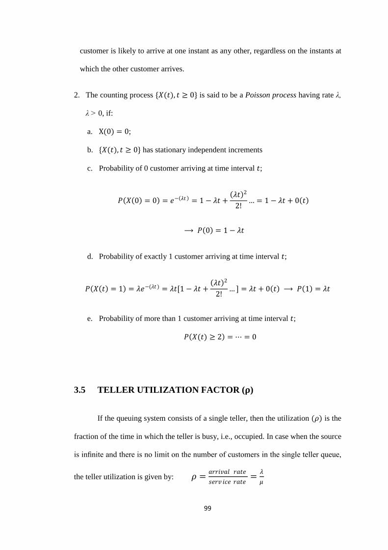
2. The counting process {𝑋𝑋(𝑡𝑡), 𝑡𝑡 ≥ 0} is said to be a Poisson process having rate λ,
λ > 0, if:
a. X(0) = 0;
b. {𝑋𝑋(𝑡𝑡), 𝑡𝑡 ≥ 0} has stationary independent increments
c. Probability of 0 customer arriving at time interval 𝑡𝑡;
𝑃𝑃(𝑋𝑋(0) = 0) = 𝑁𝑁−(𝜆𝜆𝑡𝑡 ) = 1 − 𝜆𝜆𝑡𝑡 +(𝜆𝜆𝑡𝑡)2
2!… = 1 − 𝜆𝜆𝑡𝑡 + 0(𝑡𝑡)
⟶ 𝑃𝑃(0) = 1 − 𝜆𝜆𝑡𝑡
d. Probability of exactly 1 customer arriving at time interval 𝑡𝑡;
𝑃𝑃(𝑋𝑋(𝑡𝑡) = 1) = 𝜆𝜆𝑁𝑁−(𝜆𝜆𝑡𝑡 ) = 𝜆𝜆𝑡𝑡[1 − 𝜆𝜆𝑡𝑡 +(𝜆𝜆𝑡𝑡)2
2!… ] = 𝜆𝜆𝑡𝑡 + 0(𝑡𝑡) ⟶ 𝑃𝑃(1) = 𝜆𝜆𝑡𝑡
e. Probability of more than 1 customer arriving at time interval 𝑡𝑡;
𝑃𝑃(𝑋𝑋(𝑡𝑡) ≥ 2) = ⋯ = 0
3.5 TELLER UTILIZATION FACTOR (𝛒𝛒)
If the queuing system consists of a single teller, then the utilization (𝜌𝜌) is the
fraction of the time in which the teller is busy, i.e., occupied. In case when the source
is infinite and there is no limit on the number of customers in the single teller queue,
the teller utilization is given by: 𝜌𝜌 = 𝑇𝑇𝑁𝑁𝑁𝑁𝑡𝑡𝐼𝐼𝑇𝑇𝑇𝑇 𝑁𝑁𝑇𝑇𝑡𝑡𝑁𝑁𝑠𝑠𝑁𝑁𝑁𝑁𝐼𝐼 𝑡𝑡𝑐𝑐𝑁𝑁 𝑁𝑁𝑇𝑇𝑡𝑡𝑁𝑁
= 𝜆𝜆𝜇𝜇

100
If there are more than one teller serving, the utilization factor becomes: 𝜌𝜌 = 𝜆𝜆𝑠𝑠 𝜇𝜇
,
where 𝑠𝑠 is the number of tellers. 𝜌𝜌 is used to formulate the condition for stability of
the queuing system. The condition for stability is always between zero and one,
0 ≤ 𝜌𝜌 ≤ 1. If the utilization exceeds this range then the situation is unstable and
would need additional teller(s). That is, on average the number of customers that
arrive in a unit time must be less than the number of customers that can be served.
3.6 LITTLE’S LAW
The relation between 𝐿𝐿 and 𝑊𝑊 is given by Little’s Law. Letting 𝐿𝐿 to be the
average number of customers in the queuing system at any moment of time assuming
that the steady-state has been reached, 𝐿𝐿 can be broken down into 𝐿𝐿𝑞𝑞 , the average
number of customers waiting in the queue, and 𝐿𝐿𝑠𝑠, the average number of customers
in service. Since customers in the system can only be either in the queue or in
service, it goes to show that 𝐿𝐿 = 𝐿𝐿𝑞𝑞 + 𝐿𝐿𝑠𝑠 . Likewise, 𝑊𝑊 being the average time a
customer spends in the queuing system. 𝑊𝑊𝑞𝑞 is the average amount of time spent in
the queue itself and 𝑊𝑊𝑠𝑠 is the average amount of time spent in service. As was the
similar case before, 𝑊𝑊 = 𝑊𝑊𝑞𝑞 + 𝑊𝑊𝑠𝑠. It should be noted that all averages in the above
definitions are the steady-state averages.
Defining 𝜆𝜆 as the arrival rate into the system, that is, the number of customers
arriving in the system per unit of time, it can be shown that
𝐿𝐿 = 𝜆𝜆𝑊𝑊, 𝐿𝐿𝑞𝑞 = 𝜆𝜆𝑊𝑊𝑞𝑞 , 𝐿𝐿𝑠𝑠 = 𝜆𝜆𝑊𝑊𝑠𝑠
3.7 QUEUING MODEL DESCRIPTION

101
Kendall shorthand notation is used to identify and describe the queuing
systems. The basic representation introduced by David Kendall has the form
𝐴𝐴/𝐵𝐵/𝑠𝑠/𝐾𝐾/𝑁𝑁/𝑍𝑍, where 𝐴𝐴 is the arrival time distribution, 𝐵𝐵 is the service time
distribution, 𝑠𝑠 is the number of tellers, 𝐾𝐾 is the largest possible number of customers
in the system (the capacity of the system), 𝑁𝑁 is the number of customers in the
source, and 𝑍𝑍 is the queuing discipline.
This notation can be shortened to 𝐴𝐴/𝐵𝐵/𝑠𝑠 where 𝐾𝐾 and 𝑁𝑁 are assumed to be
infinite and 𝑍𝑍 is assumed to be first-come, first-serve (FCFS). Banking queues
possess the Markovian Memoryless properties and hence 𝐴𝐴 and 𝐵𝐵 are replaced by
the two 𝑀𝑀′𝑠𝑠 to obtain the 𝑀𝑀/𝑀𝑀/𝑠𝑠 model that would be used to estimate the number
of tellers needed during each time interval.
Modelling the three main queuing systems in the case of study, that is, Single
Teller with Single-Stage Queue, Multiple Tellers with Single-Stage Queue, and
Multiple single tellers with Single-Stage Queues in Parallel, would be possible by
using 𝑀𝑀/𝑀𝑀/1 and 𝑀𝑀/𝑀𝑀/𝑠𝑠 models. These models arrival’s occur according to
Poisson process and has exponential distribution. These two assumptions are often
called Markovian properties, hence the use of the two "𝑀𝑀, 𝑠𝑠" in the notation used for
the models
3.7.1 𝑴𝑴/𝑴𝑴/𝟏𝟏 MODEL
It is the simplest realistic queue model which assumes the arrival rate follows
a Poisson distribution and the time between arrivals follows an exponential

102
distribution, has only one teller, with infinite system capacity and population, and
with First-In, First Out (FIFO) as its queuing discipline.
Consider a single stage queuing system where the arrivals are according to a
Poisson process with average arrival rate λ per unit time. That is, the time between
arrivals is according to an exponential distribution with mean 1/𝜆𝜆. For this system
the service times are exponentially distributed with mean 1/𝜇𝜇 and there is a single
teller. The service rate must be greater than the arrival rate, that is, 𝜇𝜇 > 𝜆𝜆. If 𝜇𝜇 ≤ 𝜆𝜆,
the queue would eventually grow infinitely large. Figure 3.5 shows transition
diagram for a single teller processing of a 𝑀𝑀/𝑀𝑀/1 model.
Figure 3.5 Transition diagram for a single teller processing.
Steady state probability 𝑃𝑃𝑗𝑗 of being in state 𝑗𝑗 = 0, 1, 2, … 𝑗𝑗 + 1 is:
𝑗𝑗 = 0
𝑗𝑗 = 1
𝑗𝑗 = 2⋮
𝑗𝑗𝑡𝑡ℎ 𝑁𝑁𝑞𝑞𝑁𝑁𝑇𝑇𝑡𝑡𝑡𝑡𝑜𝑜𝐼𝐼
𝜆𝜆𝑃𝑃0 = 𝜇𝜇𝑃𝑃1
(𝜆𝜆 + 𝜇𝜇)𝑃𝑃1 = 𝜆𝜆𝑃𝑃0 + 𝜇𝜇𝑃𝑃2
(𝜆𝜆 + 𝜇𝜇)𝑃𝑃2 = 𝜆𝜆𝑃𝑃1 + 𝜇𝜇𝑃𝑃3⋮
(𝜆𝜆 + 𝜇𝜇)𝑃𝑃𝑗𝑗 = 𝜆𝜆𝑃𝑃𝑗𝑗−1 + 𝜇𝜇𝑃𝑃𝑗𝑗+1
𝜆𝜆 𝜆𝜆 𝜆𝜆 𝜆𝜆 𝜆𝜆
0
2 j-1 j j+1
𝜇𝜇 𝜇𝜇 𝜇𝜇 𝜇𝜇 𝜇𝜇
𝜆𝜆 𝜆𝜆 𝜆𝜆 𝜆𝜆 𝜆𝜆
103
Putting it all together:
𝜆𝜆𝑃𝑃0 = 𝜇𝜇𝑃𝑃1,
𝑃𝑃1 = 𝜆𝜆𝜇𝜇𝑃𝑃0,
𝜆𝜆𝑃𝑃1 = 𝜇𝜇𝑃𝑃2,
𝑃𝑃2 = �𝜆𝜆𝜇𝜇�
2𝑃𝑃0,
… ,
… ,
𝜆𝜆𝑃𝑃𝑗𝑗 = 𝜇𝜇𝑃𝑃𝑗𝑗+1
𝑃𝑃𝑗𝑗 = �𝜆𝜆𝜇𝜇�𝑗𝑗𝑃𝑃0
Since
�𝑃𝑃𝑗𝑗 = 1, ⟹ 𝑃𝑃0 ��𝜆𝜆𝜇𝜇�𝑗𝑗
= 1 ⟹ 𝑃𝑃0 =1
∑ �𝜆𝜆𝜇𝜇�𝑗𝑗 ∞
𝑗𝑗=0
∞
𝑗𝑗=0
∞
𝑗𝑗=0
𝐿𝐿𝑁𝑁𝑡𝑡 𝜌𝜌 =𝜆𝜆𝜇𝜇
, 𝑡𝑡ℎ𝑁𝑁𝐼𝐼 ��𝜆𝜆𝜇𝜇�𝑗𝑗
= �𝜌𝜌𝑗𝑗 = 1 − 𝜌𝜌∞
1 − 𝜌𝜌 =
11 − 𝜌𝜌
∞
𝑗𝑗=0
, ∀ 𝜌𝜌 < 1∞
𝑗𝑗=0
Therefore, the probability of any given number of customers being in the system is
given by
𝑃𝑃0 =1
∑ 𝜌𝜌𝑗𝑗 ∞𝑗𝑗=0
= 1 − 𝜌𝜌
and 𝑃𝑃𝑗𝑗 = 𝜌𝜌𝑗𝑗 (1 − 𝜌𝜌) as the steady-state probability of state 𝑗𝑗. If 𝜌𝜌 ≥ 1, then it must
be that 𝜆𝜆 ≥ 𝜇𝜇, and if the arrival is greater than the service rate, then the state of the
system will grow without end.
The steady-state probability for this system is known, 𝐿𝐿 can now be solved.
Assuming 𝐿𝐿 is the average number of customers present in the system, waiting in
queue or being served, the formula is represented as;
𝐿𝐿 = �𝑗𝑗𝑃𝑃𝑗𝑗 =∞
𝑗𝑗=0
(1 − 𝜌𝜌)�𝑗𝑗𝜌𝜌𝑗𝑗 =∞
𝑗𝑗=0
(1 − 𝜌𝜌)𝜌𝜌�𝑗𝑗𝜌𝜌𝑗𝑗−1 ∞
𝑗𝑗=0

104
= (1 − 𝜌𝜌)𝜌𝜌𝐼𝐼𝐼𝐼𝜌𝜌
��𝜌𝜌𝑗𝑗∞
𝑗𝑗=0
� = (1 − 𝜌𝜌)𝜌𝜌𝐼𝐼𝐼𝐼𝜌𝜌
�1
1 − 𝜌𝜌�
= (1 − 𝜌𝜌)𝜌𝜌 �1
(1 − 𝜌𝜌)2� = 𝜌𝜌
(1 − 𝜌𝜌) =
𝜆𝜆 𝜇𝜇�
1 − 𝜆𝜆 𝜇𝜇�=
𝜆𝜆𝜇𝜇 − 𝜆𝜆
The average time customers spend in system, waiting plus being served 𝑊𝑊 is
𝑊𝑊 =𝐿𝐿𝜆𝜆
=𝜆𝜆
𝜇𝜇 − 𝜆𝜆 .
1𝜆𝜆
= 1
𝜇𝜇 − 𝜆𝜆
The average time customers spend in waiting in queue before service starts 𝑊𝑊𝑞𝑞 is
𝑊𝑊𝑞𝑞 = 𝑊𝑊 −1𝜇𝜇
= 1
𝜇𝜇 − 𝜆𝜆−
1𝜇𝜇
=𝜆𝜆
𝜇𝜇(𝜇𝜇 − 𝜆𝜆)=
𝜌𝜌𝜇𝜇 − 𝜆𝜆
The average time a costumer spent in service 𝑊𝑊𝑠𝑠 is
𝑊𝑊𝑆𝑆 = 𝑊𝑊 −𝑊𝑊𝑞𝑞 =1
𝜇𝜇 − 𝜆𝜆−
𝜌𝜌𝜇𝜇 − 𝜆𝜆
=1 − 𝜌𝜌𝜇𝜇 − 𝜆𝜆
The average number of customers waiting in the queue 𝐿𝐿𝑞𝑞 is
𝐿𝐿𝑞𝑞 = 𝜆𝜆𝑊𝑊𝑞𝑞 = 𝜆𝜆 .𝜆𝜆
𝜇𝜇(𝜇𝜇 − 𝜆𝜆)=
𝜆𝜆2
𝜇𝜇2(1 − 𝜆𝜆 𝜇𝜇� )=
𝜌𝜌2
1 − 𝜌𝜌

105
𝐿𝐿𝑠𝑠 can be solved to determine the average number of customers that are in service at
any given moment. In this particular system, there will be one customer in service
except for when there are no customers in the system. Thus, it can be calculated as
𝐿𝐿𝑆𝑆 = 𝐿𝐿 − 𝐿𝐿𝑞𝑞 =𝜌𝜌
(1 − 𝜌𝜌)−
𝜌𝜌2
(1 − 𝜌𝜌)=𝜌𝜌(1 − 𝜌𝜌)(1 − 𝜌𝜌)
= 𝜌𝜌
These formulas imply that it can be easy to tell how busy the teller is by just
watching the length of the queue.
3.7.2 𝑴𝑴/𝑴𝑴/𝒔𝒔 MODEL
The description of an 𝑀𝑀/𝑀𝑀/𝑠𝑠 queue is similar to that of the classic 𝑀𝑀/𝑀𝑀/1
queue except that there are 𝑠𝑠 tellers. By letting 𝑠𝑠 = 1, all the results for the 𝑀𝑀/𝑀𝑀/1
queue can be obtained. The number of customers in the system at time 𝑡𝑡, 𝑋𝑋(𝑡𝑡), in the
𝑀𝑀/𝑀𝑀/𝑠𝑠 queue can be modelled as a continuous Time Markov Chain. The condition
for stability is 𝜌𝜌 = 𝜆𝜆𝑠𝑠𝜇𝜇
< 1 where 𝜌𝜌 is called the teller utilization factor, the
proportion of time on average that each teller is busy. The total service rate must be
greater than the arrival rate, that is, 𝑠𝑠𝜇𝜇 > 𝜆𝜆. If 𝑠𝑠𝜇𝜇 ≤ 𝜆𝜆, the queue would eventually
grow infinitely large. Figure 3.6 shows a transition diagram for a multiple teller
processing of a 𝑀𝑀/𝑀𝑀/𝑠𝑠 model.
0
1
3 j-1 j j+1
2
𝜆𝜆 𝜆𝜆 𝜆𝜆 𝜆𝜆 𝜆𝜆 𝜆𝜆 𝜆𝜆 𝜆𝜆

106
Figure 3.6 Transition diagram for a multiple teller processing
Steady state probability 𝑃𝑃𝑗𝑗 of being in state 𝑗𝑗 = 0, 1, 2, … 𝑗𝑗 + 1 is:
𝑗𝑗 = 0
𝑗𝑗 = 1
𝑗𝑗 = 2
𝑗𝑗 = 3⋮
𝑗𝑗𝑡𝑡ℎ 𝑁𝑁𝑞𝑞𝑁𝑁𝑇𝑇𝑡𝑡𝑡𝑡𝑜𝑜𝐼𝐼
𝜆𝜆𝑃𝑃0 = 𝜇𝜇𝑃𝑃1
(𝜆𝜆 + 𝜇𝜇)𝑃𝑃1 = 𝜆𝜆𝑃𝑃0 + 2𝜇𝜇𝑃𝑃2
(𝜆𝜆 + 2𝜇𝜇)𝑃𝑃2 = 𝜆𝜆𝑃𝑃1 + 3𝜇𝜇𝑃𝑃3
(𝜆𝜆 + 3𝜇𝜇)𝑃𝑃3 = 𝜆𝜆𝑃𝑃2 + 4𝜇𝜇𝑃𝑃4⋮
(𝜆𝜆 + 𝑗𝑗𝜇𝜇)𝑃𝑃𝑗𝑗 = 𝜆𝜆𝑃𝑃𝑗𝑗−1 + (𝑗𝑗 + 1)𝜇𝜇𝑃𝑃𝑗𝑗+1
Putting them together to obtain,
𝜆𝜆𝑃𝑃0 = 𝜇𝜇𝑃𝑃1,
𝑃𝑃1 =𝜆𝜆𝜇𝜇𝑃𝑃0,
𝑃𝑃1 =𝜆𝜆𝜇𝜇𝑃𝑃0,
𝑃𝑃1 =𝜆𝜆𝜇𝜇𝑃𝑃0,
𝜆𝜆𝑃𝑃1 = 2𝜇𝜇𝑃𝑃2,
𝑃𝑃2 =𝜆𝜆
2𝜇𝜇𝑃𝑃1,
𝑃𝑃2 =𝜆𝜆
2𝜇𝜇�𝜆𝜆𝜇𝜇�𝑃𝑃0,
𝑃𝑃2 =12!�𝜆𝜆𝜇𝜇�
2
𝑃𝑃0,
𝜆𝜆𝑃𝑃2 = 3𝜇𝜇𝑃𝑃3,
𝑃𝑃3 =𝜆𝜆
3𝜇𝜇𝑃𝑃2,
𝑃𝑃3 = �𝜆𝜆
3𝜇𝜇� �
𝜆𝜆2𝜇𝜇� �𝜆𝜆𝜇𝜇�𝑃𝑃0,
𝑃𝑃3 =13!�𝜆𝜆𝜇𝜇�
3
𝑃𝑃0,
… ,
⋯ ,
⋯ ,
⋯ ,
𝜆𝜆𝑃𝑃𝑗𝑗 = (𝑗𝑗 + 1)𝜇𝜇𝑃𝑃𝑗𝑗+1
𝑃𝑃𝑗𝑗+1 =𝜆𝜆
(𝑗𝑗 + 1)𝜇𝜇𝑃𝑃𝑗𝑗 ,
𝑃𝑃𝑗𝑗+1 = �𝜆𝜆
(𝑗𝑗 + 1)𝜇𝜇�… �
𝜆𝜆𝜇𝜇�𝑃𝑃0
𝑃𝑃𝑗𝑗+1 =1
(𝑗𝑗 + 1)!�𝜆𝜆𝜇𝜇�𝑗𝑗+1
𝑃𝑃0,
⋯ , 𝑃𝑃𝑗𝑗+𝑘𝑘 =1
(𝑗𝑗 + 𝑘𝑘)!�𝜆𝜆𝜇𝜇�𝑗𝑗+𝑘𝑘
𝑃𝑃0, 𝑘𝑘 = 1, 2, 3, …
And in general: 𝑃𝑃𝑗𝑗 = 1𝑗𝑗 !�𝜆𝜆𝜇𝜇�𝑗𝑗𝑃𝑃0
Since
𝜇𝜇 2𝜇𝜇 3𝜇𝜇 (𝑗𝑗 − 1)𝜇𝜇 𝑗𝑗𝜇𝜇 𝑗𝑗𝜇𝜇 𝑗𝑗𝜇𝜇

107
�𝑃𝑃𝑗𝑗 = 1, ⟹ 𝑃𝑃0 ��𝜆𝜆𝑗𝑗!𝜇𝜇
�𝑗𝑗
= 1 ⟹ 𝑃𝑃0 =1
∑ � 𝜆𝜆𝑗𝑗!𝜇𝜇�𝑗𝑗 ∞
𝑗𝑗=0
∞
𝑗𝑗=0
∞
𝑗𝑗=0
Let
𝜌𝜌 =𝜆𝜆𝑠𝑠𝜇𝜇
, 𝑡𝑡ℎ𝑁𝑁𝐼𝐼 �1𝑗𝑗!�𝜆𝜆𝜇𝜇�𝑗𝑗
= �(𝑠𝑠𝜌𝜌)𝑗𝑗!
𝑗𝑗
∞
𝑗𝑗=0
, ∀ 𝜌𝜌 < 1∞
𝑗𝑗=0
The probability of any given number of customers being in the system is given 𝑃𝑃0
follows from normalization, yielding
𝑃𝑃0 = ��(𝑠𝑠𝜌𝜌)𝑗𝑗
𝑗𝑗!+
𝑠𝑠−1
𝑗𝑗=0
(𝑠𝑠𝜌𝜌)𝑠𝑠
𝑠𝑠!.
11 − 𝜌𝜌
�
−1
The probability that at any given time there are no customers waiting or being served
at steady state:
𝑃𝑃0 = ��(𝑠𝑠𝜌𝜌)𝑗𝑗
𝑗𝑗!+
𝑠𝑠−1
𝑗𝑗=0
(𝑠𝑠𝜌𝜌)𝑠𝑠
𝑠𝑠! (1 − 𝜌𝜌)�
−1
The probability that at any given time there are 𝑗𝑗 customers in the system;
If 𝑗𝑗 ≤ 𝑠𝑠 then Probability (𝑗𝑗 in system) = 𝑃𝑃0(𝑠𝑠𝜌𝜌)𝑗𝑗
𝑗𝑗 !
If 𝑗𝑗 ≥ 𝑠𝑠 then Probability (𝑗𝑗 in system) = 𝑃𝑃0𝑠𝑠𝑠𝑠𝜌𝜌𝑗𝑗
𝑠𝑠!
The expression for the average waiting time and queue lengths are fairly complicated
and depend on the probability of the average number of customers waiting in queue
to be served,

108
𝐿𝐿𝑞𝑞 =𝑃𝑃0(𝜆𝜆 𝜇𝜇⁄ )𝑆𝑆𝜌𝜌𝑠𝑠! (1 − 𝜌𝜌)2 = 𝑃𝑃0
𝑆𝑆𝑆𝑆𝜌𝜌𝑆𝑆+1
𝑆𝑆! (1 − 𝜌𝜌)2 , 𝑤𝑤ℎ𝑁𝑁𝑁𝑁𝑁𝑁 𝜌𝜌 =𝜆𝜆𝑠𝑠𝜇𝜇
The average number of customers in service 𝐿𝐿𝑠𝑠,
𝐿𝐿𝑠𝑠 = �𝑗𝑗𝑃𝑃𝑗𝑗 + �𝑠𝑠𝑃𝑃𝑗𝑗 = 𝑠𝑠𝜌𝜌∞
𝑗𝑗=𝑠𝑠
𝑠𝑠−1
𝑗𝑗=1
Now, the average number of customers in the system becomes
𝐿𝐿 = 𝐿𝐿𝑞𝑞 + 𝐿𝐿𝑠𝑠 = 𝐿𝐿𝑞𝑞 + 𝑠𝑠𝜌𝜌 = 𝐿𝐿𝑞𝑞 +𝜆𝜆𝜇𝜇
The average time customers spend in waiting in queue before service starts 𝑊𝑊𝑞𝑞 is
𝑊𝑊𝑞𝑞 = 𝐿𝐿𝑞𝑞𝜆𝜆
.
The average time customers spent waiting in the system, including service 𝑊𝑊 is
𝑊𝑊 =𝐿𝐿𝜆𝜆
=𝐿𝐿𝑞𝑞 + 𝜆𝜆
𝜇𝜇𝜆𝜆
=𝐿𝐿𝑞𝑞𝜆𝜆
+1𝜇𝜇
= 𝑊𝑊𝑞𝑞 +1𝜇𝜇
The average time a customer spent service 𝑊𝑊𝑠𝑠 is
𝑊𝑊𝑠𝑠 = 𝑊𝑊 −𝑊𝑊𝑞𝑞 = �𝑊𝑊𝑞𝑞 +1𝜇𝜇� −𝑊𝑊𝑞𝑞 =
1𝜇𝜇
3.8 DATA SHEET PROCESSING
109
For the best results, estimates of the arrival rate, service rate, departure rate
and current number of tellers should be obtained. With this information available,
data collected can be analysed from the respective banks by first keying them onto
the Microsoft Excel 2010 data table. Simple Microsoft Excel functions are the basis
for creating data tables and graphs which show the effects of customers’ arrival rate,
service time on utilization, waiting times and times customers spend in the system.
CHAPTER 4
ANALYSIS AND DISCUSSION OF RESULTS
4.0 INTRODUCTION
The 𝑀𝑀/𝑀𝑀/𝑠𝑠 queuing model is used to calculate the performance measures that are
necessary in analysing data collected. The following assumptions are made when
modelling in this environment.
1) The customers are patient (no balking, reneging, or jockeying) and come
from a population that can be considered infinite.
2) Customer arrivals are described by a poisson distribution with an average
arrival rate of 𝜆𝜆 (lambda). This means that the time between successive
customer arrivals follows an exponential distribution with an average of 1/𝜆𝜆.
3) The customer services are described by a poisson distribution with an
average service rate of 𝜇𝜇 (mu). This means that the service time for one
customer follows an exponential distribution with an average of 1/𝜇𝜇.

110
4) The waiting line priority rule used is first-come, first-serve.
The poisson distribution is a limiting case of the binomial distribution and therefore,
these two important assumptions would be necessary when dealing with poisson
process.
1) 𝜆𝜆 is constant. Each of the expected arrival rate does not change over the hour
period.
2) Independence, which means no memory and no groups. Customers do not tend
to arrive in groups. The fact that a customer just walked into the banking hall
does not make it any more or less likely that a different customer is coming
soon. If nobody comes or if ten times 𝜆𝜆 customers come, during the last time
period, the expected number of customers during the next time period is still 𝜆𝜆.
Poisson and exponential distributions are often called the Markovian properties,
hence the use of the two “M’s” in the notation used for this model. The operating
characteristics of a queuing system are calculated using 𝑀𝑀/𝑀𝑀/𝑠𝑠 queuing model
proved earlier.
4.1 PRIMARY DATA EXAMINATION
Using Microsoft 2010, raw data graphs for respective days depicting the arrival,
service and departure times of customers are drawn and shown in Appendix 1.0.

111
These graphs are plotted with number of customers against time. Customer number
starts from 0 𝑡𝑡𝑜𝑜 𝑗𝑗, where 𝑗𝑗 = 1, 2, 3, … and time begins from zero second to one hour.
From left to right part of each graph in figures 4.1 below, and all figures in Appendix
1.0, show the departure time curve followed by service time and finally, the arrival
time. The gap between arrival time and service time are wider than that of service
time and departure time except data collected on 27th April, 2012 morning that the
arrivals are not all that wider. But as the time increases, the gab between arrival and
service times widens although that of the service and departure times remain
partially constant. The graph below shows raw data graph for GCB on Wednesday,
2nd May, 2012.
Figure 4.1 Raw Data Graph for GCB on 2nd May, 2012
0:00:00
0:07:12
0:14:24
0:21:36
0:28:48
0:36:00
0:43:12
0:50:24
0:57:36
1:04:48
1 5 9 13 17 21 25 28 32
Customer Number
GCB on Wed, 2nd May, 2012, 3:00pm to 4:00pm
Customer Number Arrival Time Service Time
Teller TwoTeller One Teller Three

112
Before the data collected is analysed to see if they possess the Markovian properties,
the behaviour of customers is now studied from the graphs in figures 4.1, and all
figures in Appendix 1.0, taking into consideration some of the comments raised by
customers during observations. Some customers attributed the reasons why they
jockey, renege or balk from queue to long queues, long waiting time, network
problem, the slowness of a teller and bad attitude on the side of a staff. The tellers
also testified to the fact that some customers are impatient, assumed that they are
loyal customers and there is no need to join the queue.
Looking at customer’s behaviour from the data collection point of view, the queue
population was unlimited; there were no collusion, jockeying, reneging and balking
behaviour of customers at all the branches. There were preferential treatments for
some “special people” who receive quick services at the expense of others. Tellers
especially from Barclays and Ecobank easily vacate their cubicles at will. This
allows customers make complains after realising a long waiting time than expected.
The table below shows summary of primary data that were randomly selected
within an hour on 27th and 30th April, and 2nd May, 2012.
Table 4.1 Summary of Primary Data Collected on 27th and 30th April and 02nd
May, 2012
DATE 27th April 30th April 02nd May TIME
RANGE 8:30am - 9:30am 12:00pm – 1:00pm 3:00pm – 4:00pm
BANK BBG ECO GCB BBG ECO GCB BBG ECO GCB Number of Customers 64 30 33,35,32 48 26 26,31,30 68 31 37,35,32
Total 100 87 104

113
Number of Tellers 3 2 3 3 2 3 3 2 3
Number of
Customers served
55 23 27,26,25 45 25 25,28,27 55 28 26,26,28
Total 78 80 80
All tellers were present throughout the data collection exercise. GCB uses multiple
single tellers with single-stage Queues arrange in Parallel whilst BBG and Ecobank
use single queue to multiple tellers. 2nd May receives the highest number of
customers arriving even at the later part of the closing period of the working hours. It
was made clear by the employees that Mondays and Fridays are peak days and since
Monday, 1st May was Workers Day holiday, the following day was busier than
expected.
4.2 DISCUSSION OF FINDINGS
All data are collected within an hour. In order to have simple average calculations
throughout this analysis, an hour (01: 00: 00) would be taken as 1.00. The rate of
customer arrival at the banks fluctuates throughout the day and there might be
differences in arrivals from day to day, but it is assumed that they are independent
and identically distributed.
Changes in banking industry as a result of challenges posed by technologically
innovative competitors such as those resulting from deregulation, has seen to it that
BBG, Ecobank and GCB are fully equipped with rapid global networking, induction
of electronic banking and the rise in personal wealth have thus provided good
customer service as a key strategy for firm profitability. Hence customers from these

114
banks can transact business at any branch of their choice. Therefore, customers
arriving rate can be attributed to the size of the banking hall and the location of these
branches but not their year of establishment (i.e. whether it is an old or new branch).
These make it obvious that, the customer arriving rate at GCB, Suame Branch may
be greater than that of BBG, Tanoso Branch and Ecobank, Ash-town Branch
respectively. Throughout the three hours in three days of data collection at the
respective branches, five hundred and fifty-eight (558) customers arrived at the
selected branches, (194) in 27th April, (161) – 30th April and (203) in 2nd May, 2012.
32.26% of customers arrived at BBG, 15.59% at Ecobank whilst 52.15% at GCB.
The lowest arriving customers were recorded on 30th April for all selected branches.
It was noted that 84.05% of the arriving customers were served.
Consider the Poisson model for data collected on 30th April, 2012 in Table
A2.0 in Appendix 2.0. Lambda (𝜆𝜆) for BBG is 48.00, Ecobank, 52.00 and that of
GCB is 87.00 expected arriving customers per hour, taken one hour to be 1.00.
Using a probability limit of 0.95, by looking down the running total of the
probabilities, the first number that is bigger than or equal to 0.95 is selected. On the
side of BBG from Table A2.0, the probability, 0.9508, is in the row where number of
customers (𝑋𝑋𝑗𝑗 ) is 77, hence 0.9508 is the probability that 77 or fewer customers
would have arrived at BBG on that faithful hour and day. The table below shows the
number of customers that should have arrived at the respective banks and their
probability using a probability limit of 0.95.

115
Table 4.2 Probability of the number of customers or fewer that would have arrived
by 0.95 probability limit.
DATE BANK 𝑿𝑿𝒋𝒋 𝑷𝑷𝑷𝑷𝑷𝑷𝑷𝑷 𝑷𝑷𝒐𝒐 ≤ 𝑿𝑿𝒋𝒋
27TH APRIL
BBG 77 0.9508
ECOBANK 48 0.9514
GCB 117 0.9572
30TH APRIL
BBG 60 0.9605
ECOBANK 64 0.9547
GCB 103 0.9586
2 ND MAY
BBG 82 0.9573
ECOBANK 67 0.9504
GCB 121 0.9542
The Poisson distribution provides a realistic model for many random
phenomena and it is characterised by the mean (average arrival rate) and variance
being equal. Distribution with two different average arrival rate (𝜆𝜆) of BBG,
Ecobank and GCB for each day are plotted on the graphs in Appendix 2.0. Poisson
distribution is skewed. They may seem to be symmetrical about their average arrival
rates, but are not. The degree of skewness depends on 𝜆𝜆𝑡𝑡. The larger 𝜆𝜆𝑡𝑡 is, the more
the Poisson distribution approaches a symmetrical bell shape, the shape of the
normal distribution. The smaller 𝜆𝜆𝑡𝑡 is, the more the peak is to the left of centre.
Consider, the poisson distribution graph of data collected on 27th April, 2012
in Figure 4.2 below, the 𝜆𝜆𝑡𝑡 of GCB is greater than that of Ecobank and BBG
respectively and all their shape approach a symmetrical bell shape.

116
Figure 4.2 Poison Arrival Process for 27th April, 2012
As 𝑋𝑋𝑗𝑗 increases from 0, the probability of exactly 𝑋𝑋𝑗𝑗 arrivals rises at first. The
highest probability is at 𝑋𝑋𝑗𝑗 = 𝜆𝜆𝑡𝑡 − 1 and 𝑋𝑋𝑗𝑗 = 𝜆𝜆𝑡𝑡. According to Table A2.0 in
Appendix 2.0, for Ecobank, it was 𝑋𝑋𝑗𝑗 = 37 and 𝑋𝑋𝑗𝑗 = 38 with probability of 𝑋𝑋𝑗𝑗 being
0.5430 and 𝑋𝑋𝑗𝑗 = 99 and 𝑋𝑋𝑗𝑗 = 100 with probability of 𝑋𝑋𝑗𝑗 being 0.5266 for GCB.
After attaining a higher value of 𝑋𝑋𝑗𝑗 , the probability of 𝑋𝑋𝑗𝑗 diminishes, approaching
zero (0) as 𝑋𝑋𝑗𝑗 gets very large. Table 4.3 below shows the probability of 𝑋𝑋𝑗𝑗 , where the
curve starts to turn for all data collected.
Table 4.3 Probability of the highest turning points of the Poisson Distribution
Graphs in Appendix 2.0
-0.0100
0.0000
0.0100
0.0200
0.0300
0.0400
0.0500
0.0600
0.0700
0 8 16 24 32 40 48 56 64 72 80 88 96 104 112 120
Prob
of x
Number of Customers (x)
Poisson Arrival Process for 27th April, 2012
BBG
ECO
GCB

117
DATE BANK 𝑿𝑿𝒋𝒋 𝑷𝑷𝑷𝑷𝑷𝑷𝑷𝑷 𝑷𝑷𝒐𝒐 ≤ 𝑿𝑿𝒋𝒋
27TH APRIL
BBG 63 and 64 0.5332
ECOBANK 37 and 38 0.5430
GCB 99 and 100 0.5266
30TH APRIL
BBG 47 and 48 0.5383
ECOBANK 51 and 52 0.5368
GCB 86 and 87 0.5285
2 ND MAY
BBG 67 and 68 0.5322
ECOBANK 54 and 55 0.5358
GCB 103 and 104 0.5260
4.3 QUEUING MODEL ANALYSIS
Presentation of result on queuing analysis on data collected within April and
May, 2012 is shown in Table A3.0 in Appendix 3.0. On Table A3.0, the Total Time
involved (𝑡𝑡), Number of Customers Arrived (𝑋𝑋𝑗𝑗 ), Number of Customers Served and
the Number of Tellers (𝑠𝑠) are entered into the input section. The ‘Intermediate
Calculations’ calculates the Average Arrival Rate (𝜆𝜆) and Average Service Rate (𝜇𝜇).
‘Performance Measures’ also calculates: the Average Teller Utilization - 𝑅𝑅ℎ𝑜𝑜 (𝜆𝜆/
𝑠𝑠𝜇𝜇), Probability that the system is empty - 𝑃𝑃0, Average number of customers in the
system – 𝐿𝐿, Average number of customers in the queue - 𝐿𝐿𝑞𝑞 , Average number of
customers waiting in the service - 𝐿𝐿𝑠𝑠, Average time spent in the system – 𝑊𝑊,
Average time spent in the queue - 𝑊𝑊𝑞𝑞 and finally, the Average time a customer is
served - 𝑊𝑊𝑠𝑠. The extreme column of the table shows the unit of measurements.

118
4.3.1 PERFORMANCE ANALYSIS
One advantage of using the 𝑀𝑀/𝑀𝑀/𝑠𝑠 model is that given an arrival rate,
average service duration and the number of tellers, formulae for performance
measures such as the probability of a positive waiting time or the average waiting
time is easily obtained and implemented on a spreadsheet.
All average arriving rates are greater than the average service rate. The closer
the average service rate to the average arriving rate, the smaller utilization factor
becomes. The lowest capacity utilization of 0.35556 was recorded by BBG on 30th
April, 2012 with its arriving rate of 48.00 against its average service rate of 45.00 at
time where all tellers were available. Ecobank lowest utilisation factor of 0.59375
was also recorded on 27th April, 2012 whilst that of GCB, 0.36250 was also
recorded on 30th April, 2012. All tellers were available during data collection and
this implies that the tellers were at their best and managed to serve many customers
as possible.
All utilization factors for the data in Table A3.0 were stable. Generally, there
are two items of interest; utilization - how much time is the tellers busy or working,
and waiting time - how long do customers have to wait for service? These two items
usually conflict. As utilization (𝜌𝜌) increases, waiting time increases and vice versa.
The highest utilisation factor of 0.68750 was recorded by Ecobank on 2nd May,
followed by 0.61905 on 30th April, 2012. It was observed that the very day that the
highest utilization factor was recorded, the highest waiting time of 0.04741 was also
obtained.

119
The waiting time is measured from the time of the customer demands for
service to the time at which transaction begins (e.g. a teller is available to transact
business). It is important to note that the model’s waiting time predictions pertained
only to waiting times due to teller unavailability and do not include any other
possible waiting times prior to seeing a teller such as filling savings and debit forms
and seeing personal banker, which would have to been estimated independently. As
the number of tellers decreases, the closer the utilization approaches one. That is the
main reason why the highest utilization factors were recorded at Ecobank on 2nd
May and 30th April, 2012 respectively, when there were only two tellers working.
The greater the capacity utilization factor, the smaller the probability of the
system to be empty and as the probability increases, the more probability of the
number of customers in the entire queuing system approaches zero. Table 4.4 shows
the highest probability that a customer and three customers are in the Queuing
system as depicted in Figure 4.5 below and all figures in Appendix 3.0. The
probability that there are no customers in the system is given in Table A3.0.
Table 4.4 Probability that a customer and five customers are in the Queuing system
Highest Probability that a customer is in
the system
Probability that three customers are in the
system DATE BANK 𝑿𝑿𝒋𝒋 𝑷𝑷𝑷𝑷𝑷𝑷𝑷𝑷 𝑷𝑷𝒐𝒐 𝑿𝑿𝒋𝒋 𝑿𝑿𝒋𝒋 𝑷𝑷𝑷𝑷𝑷𝑷𝑷𝑷 𝑷𝑷𝒐𝒐 𝑿𝑿𝒋𝒋
27TH APRIL
BBG 1 0.30584 3 0.08032 ECOBANK 1 0.25490 3 0.10671 GCB 1 0.26902 3 0.09448
30TH BBG 1 0.33905 3 0.06858
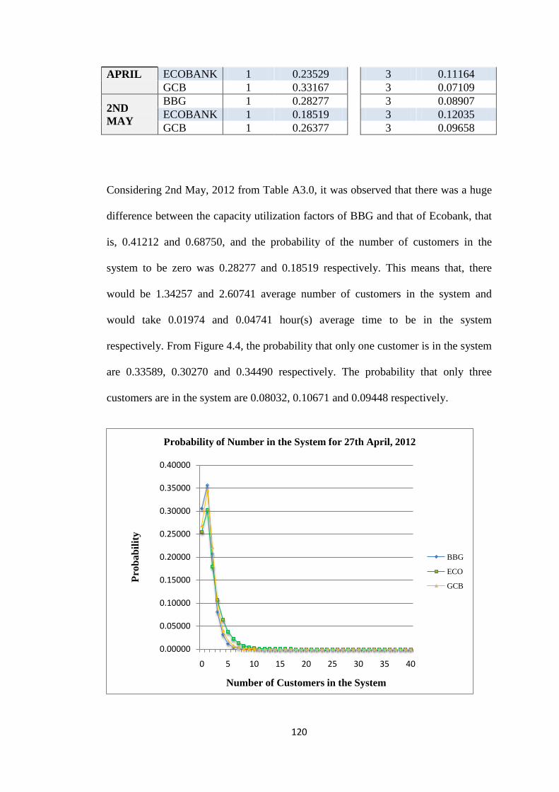
120
APRIL ECOBANK 1 0.23529 3 0.11164 GCB 1 0.33167 3 0.07109
2ND MAY
BBG 1 0.28277 3 0.08907 ECOBANK 1 0.18519 3 0.12035 GCB 1 0.26377 3 0.09658
Considering 2nd May, 2012 from Table A3.0, it was observed that there was a huge
difference between the capacity utilization factors of BBG and that of Ecobank, that
is, 0.41212 and 0.68750, and the probability of the number of customers in the
system to be zero was 0.28277 and 0.18519 respectively. This means that, there
would be 1.34257 and 2.60741 average number of customers in the system and
would take 0.01974 and 0.04741 hour(s) average time to be in the system
respectively. From Figure 4.4, the probability that only one customer is in the system
are 0.33589, 0.30270 and 0.34490 respectively. The probability that only three
customers are in the system are 0.08032, 0.10671 and 0.09448 respectively.
0.00000
0.05000
0.10000
0.15000
0.20000
0.25000
0.30000
0.35000
0.40000
0 5 10 15 20 25 30 35 40
Prob
abili
ty
Number of Customers in the System
Probability of Number in the System for 27th April, 2012
BBG
ECO
GCB

121
Figure 4.4 Probability of a number of customers in the System for 27th April,
2012
From the results obtained, the highest capacity utilization of 0.68750
obtained at Ecobank on 2nd May, 2012 has an average number of customers waiting
in queue to be 1.23241 customers, 1.37500 average number of customers in the
service at a point in time, with an average waiting time in the queue and in the
queuing system to be 0.02241 hour(s) and 0.04741 hour(s) respectively.
Assuming there is one teller, two tellers, three tellers and four tellers,
comparing their performance measures and to making policy recommendations,
taking into consideration, the average arrival rate, 𝜆𝜆 = 52.00 and service rate,
𝜇𝜇 = 36.00, Table 4.5 presents the results for considering one to four tellers at a
given time.
Table 4.5 Presentation of results for considering one to four tellers at a given point
in time
Model Type M / M / 1 M / M / 2 M / M / 3 M / M / 4 Performance Measures
Rho (𝜌𝜌) 1.44444 0.72222 0.48148 0.36111 Probability the system is empty, 𝑃𝑃0 -0.44444 0.16129 0.22440 0.23398 Average number in the system, 𝐿𝐿 -3.25000 3.01935 1.64629 1.48199 Average number waiting in the queue, 𝐿𝐿𝑞𝑞 -4.69444 1.57491 0.20185 0.03755 Average time in the system, 𝑊𝑊 -0.06250 0.05806 0.03166 0.02850 Average time in the queue, 𝑊𝑊𝑞𝑞 -0.09028 0.03039 0.00388 0.00072 Average time a customer is served, Ws 0.02778 0.02778 0.02778 0.02778

122
Average number waiting in the service,𝐿𝐿𝑠𝑠 1.44444 1.44444 1.44444 1.44444
From the Table 4.5, it was observed that, as the number of tellers’ (𝑠𝑠) increase, the
teller utilization factor (𝜌𝜌) increases, increasing the probability that a system is
empty (𝑃𝑃0) and hence the good the performance measures. The average number of
customers waiting in the service and time they are served remain constant throughout
all the model types. The inappropriateness of a single teller model (𝑀𝑀/𝑀𝑀/1) to
solve customer-waiting problems becomes apparent as the utilization factor of
1.4444 becomes unstable as a result of the arrival rate (𝜆𝜆) being greater than the
service rate (𝜇𝜇). The remaining performance indicators under the model type
(𝑀𝑀/𝑀𝑀/1) revealed negative times and number of customers. But there is no
negative number of customers waiting at a negative time in the queue.
It is therefore much prudent to increase the number of tellers to have a stable
utilization factor. However, multi-teller models were compared and it was observed
that;
a) Using a model type with three-teller system is better than a two-teller system
in all complicating result. For instance, assuming that there are three tellers
serving the arriving customers, there will be 1.64629 customers waiting in
queue instead of 3.01935 customers; a customer will spend 0.03166 hour(s)
in the system instead of 0.05806 hour(s). A three-teller system has a high
probability of being idle 0.22440 than two-teller system.

123
b) If all facilities are available, then a four-teller system will be preferable than
three and two-teller system.
CHAPTER 5
SUMMARY, RECOMMENDATIONS AND
CONCLUSION
5.0 INTRODUCTION
This chapter concludes the analysis and gives recommendation that would be
necessary to reduce capacity utilization of facilities, enhancing free movement of
customers and reduction of time a customer spends at the banking hall.
5.1 SUMMARY OF FINDINGS
Out of five hundred and fifty-eight (558) customers arriving at the two banks,
84.05% customers were served, 52.15% of them transacted business with GCB,
32.26% with BBG whilst 15.59% with Ecobank. The average arriving number of
customers per hour each day for the three day data collection period was 60, 29 and
97 customers for BBG, Ecobank and GCB respectively.
Network constraints and tellers are considered to be the cause of long
queuing especially at GCB as some tellers work at a slow pace and easily vacate

124
their cubicles to do other business within the bank while customers keep waiting.
Since the study concentrated on queues within the bank only, it was very difficult to
identify customers balking but there were some jockeying behaviour of customers
recorded with no reneging.
The data collected possess the Markovian properties and was capable to be
analysed with the queuing model 𝑀𝑀/𝑀𝑀/𝑠𝑠. All average arriving rates (λ) are greater
than the average service rate (µ). The closer the average service rate to the average
arriving rate, the smaller utilization factor becomes. The greater the capacity
utilization factor, the smaller the probability of the system to be empty and as the
probability increases, the more the probability of the number of customers in the
entire queuing system approaches zero. 2nd May,2012, was the busiest day among
the selected data collection days at all selected branches.
Considering one-teller system up to four-teller system, the average number of
customers waiting in the system and time they are served remain constant from one
teller to four tellers. The inappropriateness of a single teller model for solving
customer-waiting problems becomes apparent as it shows negative figures for all
performance criteria except 𝑊𝑊𝑠𝑠 and 𝐿𝐿𝑠𝑠. If facilities are available, then a four-teller
system would be preferable than three and two-teller system.
5.2 CONCLUSION

125
With the knowledge of probability theory and stochastic process, it is
possible to derive many different queuing models, including but not limited to the
ones we observed in this study.
It was observed that the trade-offs between utilization of the present capacity
level in the banking industry was easily seen by making better decisions relating to
tellers and potential waiting times for customers. It also uncovered the applicability
and extent of usage of queuing models in achieving customer satisfaction at lowest
cost.
There were consistency in the number of tellers at GCB but there were
several times that the number of tellers at BBG and Ecobank were reduced to either
two or one, resulting in long queues and the recording of the highest capacity
utilization factors at Ecobank. Based on the data collected, Monday and Fridays
confirm to be the peak days of the week.
5.2 RECOMMENDATION TO STAKEHOLDERS
Based on the conclusion of this study, the following recommendations are
suggested for efficiency improvement and quality of service to customers in the
selected branches and the banking industry as a whole:
1. It is clear that during peak times, the moment the number of tellers is reduced
to less than three; it exerts unnecessary pressure in the banking hall, and on
the entire queuing system and staff of the bank. Hence, increasing the
capacity utilization on the banking facilities. It is recommended that any time

126
a teller is at break or is on leave, especially at peak periods, managers should
replace them to avoid time delays due to long queue of customers.
2. Tellers must be well equipped with fast computers, uninterrupted network
service and must be trained to work fast as much as possible. It was observed
that as the average time a customer is served by a teller (𝑊𝑊𝑠𝑠) decreases, the
average number of customers in the system (𝐿𝐿𝑠𝑠) also decreases and hence a
good performance measures.
3. The queue characteristics should be viewed from a strategic point by
managers or director of operations as to whether the waiting time is
reasonable and acceptable by increasing the number of tellers to reduce the
capacity utilization factor and unnecessary pressure at the banking hall if and
only if the facilities are available.
For instance, since the banking halls of BBG, Tanoso and Ecobank, Ash-
town Branches are very small, the management should always increase the
number of tellers to four or three respectively to reduce the average time a
customer spends in the banking hall.
4. Introduction to banking ethics, communication skills and regular training of
employees to enable them to eliminate unnecessary delays when serving a
customer for a better improvement of staff-customers relationship.
5. Conjecture of customers on queues seems to be very common at GCB. The
manger should provide queuing guards in order to prevent the rampant
walking around and jockeying of customers inside the banking hall.
5.3 RECOMMENDATION TO FUTURE RESEARCHERS

127
It is important to note that the model’s waiting time predictions pertain only
to waiting time due to teller unavailability and do not include any other possible
waiting times prior to seeing a teller such as filling savings and debit forms and
enquiries times, which would have to be estimated separately. I therefore recommend
to future researchers to work on the total time a customer spends in the banking hall,
taking into account time the customer enters the bank but not the queue and the time
he/she departs from the banking hall irrespective of what transactions the customer
deals at the bank.
The challenges posed by customers on technologically innovative subsidiary
channels such as the Automated Teller Machines (ATMs), Internet, Mobile and
Telephone banking cannot be left out and need thorough queuing analysis on their
queuing systems.
The applications of queuing theory extend well beyond waiting line at the
banking industry. It may take some creative thinking, but if there is any sort of
scenario where time passes before a particular event occurs, there is probably some
way to develop it into a queuing model. Queues are so commonplace in society that
it is highly worthwhile to study them, even if only a few seconds off one’s wait in the
check line.
BIBLIOGRAPHY
Agboola A. A and Salawu R. O.(2008), “Optimizing the Use of Information and
Communication Technology (ICT) in Nigerian Banks”, Journal of Internet
Banking and Commerce, Vol. 13, no.1, pp. 4-15

128
Ankaah, K. N. (1995), “Banks as providers of funds for building business,” The
Ghanaian Banker, Journal of the chartered Institute of Bankers Ghana, pp. 6.
Ashley D.W. (2002), “Introduction to Waiting Line Models” available at,
http/www.google.com.
Armero, C. (1994), “Bayesian inference in Markovian queues”, pp. 419-426.
Bailey, N. T. J. (1954), “A continuous time treatment of a simple queue using
generating functions”, J. Roy. Statist. Soc. B, 16, pp. 288-291.
Baker S.L. (2006), “Queuing Theory Cookbook” Lect. Notes,
hspm.sph.sc.edu/courses/716.html
Bale, A.F. (2002), “Managerial Applications of Queuing Models in the Service
Industry: A Case Study of Afribank Nigeria Plc., Ilorin Main Branch”. A Research
Paper submitted to Bus. Admin. Dep’t, University of Ilorin, Ilorin.
Barrer, D.Y. (1957), “Queuing with impatient customers and ordered service”,
Operation Research 5, pp. 650-656.
Basawa, I. V. and Prabhur, N. U. (1988), “Large sample inference from single
server queues”, Queueing Systems, 3, pp. 289-306.
Bassett, G. (1992), “Operations Management for Service Industries: Competing in
the Service Era”, Quorum Books.
Benjamin A.I, Levy H. and David, R. (2004), “Quantifying fairness in queueing
systems: principles and applications”, Rutcor Research Report, New Jersey, pp. 3-6

129
Bhat, U. N. and Basawa, I. V. (2002), “Maximum likelihood estimation in queuing
systems”, Advances on Methodological and Applied Aspects of Probability and
Statistics, (Ed. N. Balakrishnan), Taylor & Francis, N.Y., pp. 13-29.
Billingsley, P. (1961), “Statistical Inference for Markov Processes”, University of
Chicago Press.
Brewton, J.P. (1989), “Introduction to Probability Models”, 18 Ed, University of
Columbia Academic Press, pp. 22-24.
Brockmeyer, E., Halstrom and H. L., Jensen, A. (1960), “The Life and Works of A.
K. Erlang, Acta Polytechnica Scandinavica, Applied Math. and Comp. Machinery”,
Series No. 6, Copenhagen.
Cidon I., Guerin R., Khamisy A. and Sidi M. (1991), “On queues with inter-arrival
times proportional to service times”, Tech. Rept. EE PUB. No. 811, Technion.
Clarke, A. B. (1957), “Maximum likelihood estimates in a simple queue”, Ann.
Math. Statist., 28, pp. 1036-1040.
Elegalam (1978), “Customer retention versus cost reduction technique” A paper
presented at the Bankers forum held at Lagos, pp.9-10.
Fry, T. C. (1928), “Probability and its Engineering Uses”, Van Nostrand Co.
Gaver, D. P. Jr. (1968), “Diffusion approximations and models for certain
congestion problems”, J. Appl. Prob. 5, pp. 607-623.
Goyal, T. L. and Harris, C. M. (1972), “Maximum likelihood estimation for queues
with state dependent service”, Sankhya A34, 65-80.

130
Heyman, D. P. (1968), “Optimal operating policies for M/G/1 queueing systems”,
Operations Res.16, 362-382.
Hillier, F. S. (1963), “Economic models for industrial waiting line problems”,
Management Sci. 10, 119-130.
Iglehart, D. L. and Whitt, W. (1970), “Multiple channel queues in heavy traffic I”,
Adv. Appl. Prob., 2, pp. 150-177.
Incoom, S. E. (1998), “Regulation and Supervision.” The monetary and financial
system bankers’ workbook series, C.I.B., Accra, pp. 227 – 234.
Jackson, J. R. (1957), “Networks of waiting lines”, Oper. Res. 5, pp. 518-521.
Kapstein, E.B. (1991), “Supervision International Banks, Origins and Implications
of the Basle Accord”, Essays in international finance, No. 185, pp. 1-14.
Klinrock, L. (1976), “Queueing Systems Vol. II: Computer Applications”, John
Wiley & Sons, New York.
Ledermann, W. and Reuter, G. E. (1956), “Spectral theory for the differential
equations of simple birth and death processes,” Phil. Trans. Roy. Soc., London
A246, pp. 321-369.
Leonard, K. (1975), “Queueing Systems” Vol. 1, John Wiley and Sons, New York.
Lewis, B. R., Orledge J. and Mitchell, B.S (1994), “Service quality: Students
assessment of banks and societies”, International Journal of Bank Marketing, Vol.
12, No.4, pp. 3-12.
131
Lindley, D. V. (1952), “The theory of queues with a single server”, Proc. Comb.
Phil. Soc. 48, pp. 277-289.
Mitchell, C.R, Paulson A.S. and Beswick C.A. (1977), “The effect of correlated
exponential service times on single server tandem queues”, Naval Research
Logistics Quaterly 24 pp. 95–112.
Molina, E. C. (1927), “Application of the theory of probability to telephone
trunking problems”, Bell System Tech. J. 6, pp. 461-494.
Oladapo A. (1988), “Relationship between Arrival Rates of Customers and Bank’s
Service Rates”, Seminar Paper Series, University of Ife.
Olaniyi T.A. (2004), “An appraisal of Techniques for minimizing cost of customers
waiting in first bank of Nigeria Plc Ilorin”, Ilorin Journal of Business and Social
Science, Vol.9, No. 1&2, pp. 139-145.
Pollaczek, F. (1934), “Uber das Warteproblem”, Math. Zeitschrift, 38, pp. 492-537.
Pollaczek, F. (1965), “Concerning an analytical method for the treatment of
queuing problems”, Univ. of North Carolina, Chapel Hill, pp. 1-42.
Rao, S. S., Bhat, U. N. and Harishchandra, K. (1984), “Control traffic intensity in a
queue - A method based on SPRT”, O.R 21, pp. 63-80.
Borst S.C., Boxma O.J., and Comb´e M.B(1993), “An M/G/1 queue with customer
collection”, Comm. Statist. Stochastic Models 9 pp. 341–371.
Saaty, T. L. (1961), “Elements of Queueing Theory and Applications”, Mc-Graw
Hill Book Co., New York.

132
Syski, R. (1960), “Introduction to Congestion Theory in Telephone Systems, Oliver
and Boyd”, London.
Travis C. and Michael M. (2007), “Analysis of Teller Service Times in Retail
Banks” University of North Texas, CS-BIGS, pp. 16-25
Wenny C. and Whitney C. (2004), “Determining Bank Teller Scheduling using
Simulation with Changing Arrival Rates”, J.O.M, pp. 1-8
William S. (2000), “Queuing Analysis”, www.WilliamStallings.com, pp 1-18.
Whittle, P. (1968), “Equilibrium distributions for an open migration process”, J.
Appl. Prob. 5, 567-571.
Wolff, R. W. (1965), “Problems of statistical inference for birth and death queueing
models”, Operations Res. 13, 343-357.