SCOR Switzerland Ltd Audit Committee Meeting August 28, 2012

Kurtosis and skewness estimation for non-life reserve risk distribution ASTIN colloquium 2013 Eric Dal Moro

2

Disclaimer

Any views and opinions expressed in this presentation or any material distributed in conjunction with it solely reflect the views of the author and nothing herein is intended to, or should be deemed, to reflect the views or opinions of the employer of the presenter.

The information, statements, opinions, documents or any other material which is made available to you during this presentation are without any warranty, express or implied, including, but not limited to, warranties of correctness, of completeness, of fitness for any particular purpose.

3

SCOR Internal Model - P&C

Group

LOB1 LOB2

New Bus Unearned

Treaty P Treaty NP Fac.

LE1 LE2

Reserves

Treaty P Treaty NP Fac.

LE1 LE2

LeafNode

1

MarginalSim. Loss

MarginalSim. Prem

MarginalSim. Exp

Determ.Patterns

LeafNode2

MarginalSim. Loss

Determ.Patterns

Clayton copula calibrated via Probex

4

0.00%

2.00%

4.00%

6.00%

8.00%

10.00%

12.00%

12'000'000 14'000'000 16'000'000 18'000'000 20'000'000 22'000'000 24'000'000 26'000'000 28'000'000 30'000'000

5

Agenda

Reserve risk distribution – What do we know ?

Skewness and kurtosis – Some basic properties

Reserve risk distribution – A proposal for a new approach

Simulations to the ultimate

Application to real triangles

The Johnson distribution

Conclusion

References

6

1 2 3 4 5

1 C1,1 C1,2 C1,3 C1,4 C1,5

2 C2,1 C2,2 C2,3 C2,4

3 C3,1 C3,2 C3,3

4 C4,1 C4,2

5 C5,1

UWY Dvpt Ultimate

Reserve risk distribution – What do we know in a chain-ladder framework ?

11 , ˆ

1,

11,

I-kC

Cf kI

jkj

kI

jkj

k ≤≤=∑

∑−

=

−

=+

21 ˆ

11ˆ

2

1 ,

1,,

2 I-kfor fC

CC

kI

kI

ik

ki

kikik ≤≤

−

−−= ∑

−

=

+σ

∑=

I

jIjC

1,

ˆ ∑ ∏∑= +−=

+−=

=I

j

I

jIkkjIj

I

jIj fCC

1 11,

1,

ˆˆ

IC ,1ˆ

IC ,2ˆ

IC ,3ˆ

IC ,4ˆ

IC ,5ˆ Best Estimate

1,,ˆˆ

+−−= jIjIjj CCR

Reserves

From Mack (1993):

( )

( )

+=

+=

∑∑

∑ ∑∑

∑∑

−

=

−

−+=

=

−

−+=−

=

+==

kI

nnk

ki

I

iIk k

kIii

I

i

I

iIkkI

nnk

k

kI

ijIjIii

I

ii

CCfCRmse

with

C

fCCRmseRmse

1

,

1

12

22,

2

1

1

1

2

2

1,,

2

1ˆ1

ˆˆˆˆ

(1) ˆ

ˆ2ˆˆˆˆ

σ

σ

7

Reserve risk distribution – What do we know in other frameworks ?

Bornhuetter – Ferguson

Best estimate known

Estimate of the standard deviation known (see Mack 2008)

Mix Bornhuetter – Ferguson / Chain-ladder

Best estimate known

Hybrid chain-ladder method provides an estimate of the standard deviation (see Arbenz 2010)

GLM based on incremental triangles

Best estimate known

Different estimates of the standard deviation given (See Merz-Wüthrich 2008)

Cape-Cod

Best estimate known

No estimate of the standard deviation

8

Reserve risk distribution – How do we get the distribution today ?

Assume a lognormal distribution with mean given by Best Estimate and standard deviation given by Mack standard equation (see equation (1) on slide 3).

Bootstrapping techniques based on Pearson residuals (see England and Verall 2006)

Generalized Linear Models based on incremental triangles (see Merz and Wüthrich 2008)

Usual assumption: The distribution of the random element of the incremental claim Xi,j belongs to the Exponential Dispersion Family (e.g. Poisson, Gamma …)

Model of Salzman, Wüthrich, Merz on higher moments of the Claim Development Result in General Insurance (ASTIN Bulletin 2012)

Two models assumed for the distribution of the individual claims development factor : Gamma and Lognormal models

All of the above models use some distributional assumptions.

ji

jiji C

CF

,

1,,

+=

9

Skewness and kurtosis – Some basic properties

The following properties are taken from Wikipedia:

The skewness of a random variable X is the third standardized moment, denoted γ1 and defined as

where µ3 is the third moment about the mean µ and σ is the standard deviation.

33

3

1 σµ

σµγ =

−

=XE

10

Skewness and kurtosis – Some basic properties

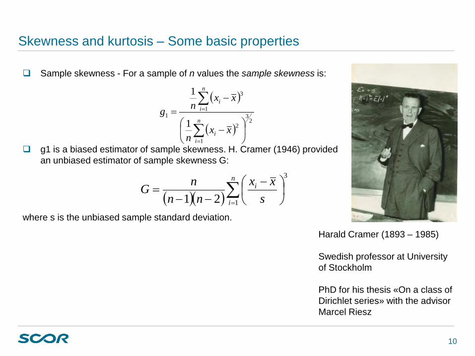
Sample skewness - For a sample of n values the sample skewness is:

g1 is a biased estimator of sample skewness. H. Cramer (1946) provided an unbiased estimator of sample skewness G:

where s is the unbiased sample standard deviation.

( )

( )2

3

1

2

1

3

11

1

−

−=

∑

∑

=

=

n

ii

n

ii

xxn

xxng

( )( )∑=

−

−−=

n

i

i

sxx

nnnG

1

3

21

Harald Cramer (1893 – 1985) Swedish professor at University of Stockholm PhD for his thesis «On a class of Dirichlet series» with the advisor Marcel Riesz

11

Skewness and kurtosis – Some basic properties

The fourth standardized moment is defined as

where µ4 is the fourth moment about the mean µ and σ is the standard deviation.

Excess kurtosis is defined as:

44

4

2 σµ

σµβ =

−

=XE

344

2 −=σµγ

Excess kurtosis Leptokurtic: D: Laplace distribution S: Hyperbolic secant distribution L: Logistic distribution N: Normal distribution Platykurtic: C: Raised cosine distribution W: Wigned semicircle distribution U: Uniform distribution

12

Skewness and kurtosis – Some basic properties

For a sample of n values the sample excess kurtosis is

g2 is a biased estimator of the sample excess kurtosis. H. Cramer (1946) provided an “unbiased” estimator of sample excess kurtosis as follows. We denote :

Then an unbiased estimator of the fourth centered moment is:

( )

( )3

1

1

2

1

2

1

4

2 −

−

−=

∑

∑

=

=

n

ii

n

ii

xxn

xxng

( )∑=

−=n

ii xx

nm

1

44

1 ( )∑=

−=n

ii xx

nm

1

22

1

( )( )( )( )

( )( )( )( )321

323321

32 224

2

4 −−−−

−−−−

+−=

nnnnnmm

nnnnnnM

13

Reserve risk distribution – A proposal for a new approach

1 2 3 4 5

1 C1,1 C1,2 C1,3 C1,4 C1,5

2 C2,1 C2,2 C2,3 C2,4

3 C3,1 C3,2 C3,3

4 C4,1 C4,2

5 C5,1

UWY Dvpt Ultimate

∑=

I

jIjC

1,

ˆ

IC ,1ˆ

IC ,2ˆ

IC ,3ˆ

IC ,4ˆ

IC ,5ˆ

( )( )[ ] 2

3,1,1,

,1,1,

,...,|

,...,|

kiiki

kiiki

CCCVar

CCCSK

+

+Assumption on skewness : depends on k but not on i where:

For one development year the skewness/kurtosis is the same for any UWY. Context : Reserving portfolio which risks are similar for every UWY.

( ) ( )( )[ ]kiikiikikikiiki CCCCCECECCCSK ,1,3

,1,1,1,,1,1, ,...,|,...,|,...,| +++ −=

( )( )[ ]2,1,1,

,1,1,

,...,|,...,|

kiiki

kiiki

CCCVarCCCKT

+

+Assumption on kurtosis: depends on k but not on i where: ( ) ( )( )[ ]kiikiikikikiiki CCCCCECECCCKT ,1,

4,1,1,1,,1,1, ,...,|,...,|,...,| +++ −=

14

Skewness : Use of the new approach

With the above assumption, under a Mack model for the volatility, we have: ( )

( )[ ]( )[ ]

( ) [ ] 23

,32

3

,2

k,1,1,

23

,2

,1,1,

23

,1,1,

,1,1,k

,...,|

,...,|

,...,|

,...,|such that

kikkikkiiki

kik

kiiki

kiiki

kiikik

CSkCCCCSK

C

CCCSK

CCCVar

CCCSK

==⇒

==∃

+

+

+

+

σγ

σγγ

Then, it is possible to show that the estimator below is unbiased.:

31for ˆ1ˆ3

1 ,

1,23

3

1,

2

1

23

,

3,

I-k fC

CC

C

CkI

kSkI

ik

ki

ki

kI

iki

kI

iki

k ki≤≤

−

−−

= ∑

∑

∑

−

=

+

−

=

−

=

Comments: 1 – The formula for has a similar “shape” as the formula for 2 – The formula for uses the usual weighted average (power 1.5) of cubic differences. 3 – As for the formula of , outliers can play a major role in the estimation of 4 – The homogeneity formulas in terms of power of Ci,k is kept in the above formulas.

3ˆkkS 2ˆ kσ3ˆkkS

2ˆ kσ 3ˆkkS

15

Kurtosis : Use of the new approach

With the above assumption, under a Mack model for the volatility, we have: ( )

( )[ ]( )

[ ]( ) [ ] 2

,42

,2

k,1,1,

2,

2

,1,1,2

,1,1,

,1,1,k

,...,|

,...,|

,...,|,...,|

such that

kikkikkiiki

kik

kiiki

kiiki

kiikik

CKtCCCCKT

C

CCCKTCCCVarCCCKT

==⇒

==∃

+

+

+

+

σγ

σγγ

Then, it is possible to show that the estimator below is unbiased.:

Notes: 1 – The formula is “as expected”. 2 – There is the “usual correction” equal to 3 times the square of the variance estimator. 3 – The homogeneity formulas in terms of power of Ci,k is kept in the above formulas.

( )

41for

1

462ˆ3ˆ

ˆ

4

1,

1

4,

2

1

2,

1

4

1,

,

3

1,

1

3,

2

1,

1

2,

22

4

1 ,

1,2

4

,

I-k

C

CC

C

C

C

C

C

Cf

CC

C

tK

kI

iki

kI

iki

kI

ikikI

ikI

iki

ki

kI

iki

kI

iki

kI

iki

kI

iki

k

kI

ik

ki

ki

k

ki

≤≤

−

+

−

+

−−

−

=

∑

∑∑∑

∑

∑

∑

∑

∑∑

−

=

−

=

−

=−

=−

=

−

=

−

=

−

=

−

=−

=

+ σ

16

Skewness/Kurtosis : Simulation to the ultimate

1 2 3 4 5

1 C1,1 C1,2 C1,3 C1,4 C1,5

2 C2,1 C2,2 C2,3 C2,4

3 C3,1 C3,2 C3,3

4 C4,1 C4,2

5 C5,1

UWY Dvpt Ultimate

11 , ˆ

1,

11,

I-kC

Cf kI

jkj

kI

jkj

k ≤≤=∑

∑−

=

−

=+

21 ˆ

11ˆ

2

1 ,

1,,

2 I-kfor fC

CC

kI

kI

ik

ki

kikik ≤≤

−

−−= ∑

−

=

+σ

∑=

I

jIjC

1,

ˆ

IC ,1ˆ

IC ,2ˆ

IC ,3ˆ

IC ,4ˆ

IC ,5ˆ

31for ˆ1ˆ3

1 ,

1,23

3

1,

2

1

23

,

3,

I-k fC

CC

C

CkI

kSkI

ik

ki

ki

kI

iki

kI

iki

k ki≤≤

−

−−

= ∑

∑

∑

−

=

+

−

=

−

=

Supporting distribution to estimate the distributional properties of Ci,I. ⇒ Recursive calculation

(see Mack 1999)

Assumption: The chosen supporting distribution should not be influencing the overall simulated skewness.

4ˆktK

17

i Ci1 Ci2 Ci3 Ci4 Ci5 Ci6 Ci7 Ci8 Ci9 Ci10

ξ2 ξ3 ξ4 ξ5 ξ6 ξ7 ξ8 ξ9 ξ10Asymmetry

6

7

8

9

10

2

3

4

5

Skewness/Kurtosis : Simulation to the ultimate – Generalized Pareto Distribution

);;(ˆ,,, kkikiki sGPDC ζµ∝

Parameters of all distributions at step k are known

Estimation of parameters of all distributions at

step k+1

( ));;(

1ˆ,,

,,,, kkiki

k

kikikiki sGPD

UsC

k

ζµζ

µζ

∝−

+=−

( )

312112

ˆˆ

1

113

1

31

1+

++

+

++ −

−+==

k

kk

k

kk

kSζ

ζζσ

ξ

( ) ( )12

1

21,

1,

,2,1, 211

ˆ1ˆˆˆ

++

+−

=

+ −−=

+=

∑ kk

kikI

jkj

kikkiki

s

C

CCarianceV

ζζσ

1

1,1,,1, 1

ˆˆˆ+

+++ −+==

k

kikikikki

sCfC

ζµ

( )( )( )2

11

311

221

41

1271453 3

ˆ

ˆ

++

++

+

+

+−−−

=kk

kk

k

ktKζζζζ

σ

18

Application to real triangles

The calculations of Skewness/Kurtosis per development year as well as the simulations to ultimate on the triangle using the GPD distribution were performed on the following triangle:

Schedule P triangles provided by G Meyers on the CAS website – Accident year 1988 to 1997 (10 x 10 triangles - http://www.casact.org/research/index.cfm?fa=loss_reserves_data):

Farmers Alliance – Private Motor

NC Farm Bureau – Private Motor

New Jersey Manufacturers – Private Motor

Pennsylvania – Product Liability

West Bend – Product Liability

First example triangle in Mack 1993 (10 x 10 triangle)

SCOR Global P&C 2011 reserve triangles – Excel files (15x15 triangle - http://www.scor.com/en/investors/financial-reporting/presentations.html)

Casualty proportional worldwide

Motor non-proportional worldwide

19

Application to real triangles – Skewness and Kurtosis per development year – 10x10 triangles

1 2 3 4 5 6 7

0.611 -0.256 -0.349 -0.090 1.049 0.477 0.273

317.02% 177.30% 166.23% 146.75% 340.69% 165.38% NA

0.703 0.412 0.727 -0.047 -0.058 -0.769 0.500

223.54% 201.65% 182.26% 78.01% 144.84% 237.28% NA

0.583 0.187 0.414 -0.565 -0.141 0.230 -0.008

204.32% 229.15% 207.06% 192.21% 103.56% 104.25% NA

0.774 1.716 -0.540 -1.059 -0.620 0.164 0.111

324.61% 620.07% 298.72% 369.19% 164.25% 119.36% NA

-0.008 1.060 0.525 -0.507 -0.030 -0.484 -0.113

205.13% 411.28% 302.64% 200.90% 125.54% 121.50% NA

0.137 0.215 0.638 -0.433 0.402 -0.026 -0.497

184.92% 170.29% 265.62% 162.92% 185.65% 123.00% NA

Mack 1993

Private MotorNew Jersey

Manufacturers

Product Liability Pennsylvania

Product Liability West Bend

k

Private Motor Farmers Alliance

Private Motor NC Farm Bureau

( )224 ˆ/ˆkktK σ

( ) 2323 ˆ/ˆ

kkkS σ

( )224 ˆ/ˆkktK σ

( ) 2323 ˆ/ˆ

kkkS σ

( )224 ˆ/ˆkktK σ

( ) 2323 ˆ/ˆ

kkkS σ

( )224 ˆ/ˆkktK σ

( ) 2323 ˆ/ˆ

kkkS σ

( )224 ˆ/ˆkktK σ

( )224 ˆ/ˆkktK σ

( ) 2323 ˆ/ˆ

kkkS σ

( )224 ˆ/ˆkktK σ

( )224 ˆ/ˆkktK σ

( ) 2323 ˆ/ˆ

kkkS σ

( )224 ˆ/ˆkktK σ

20

Application to real triangles – Skewness and Kurtosis per development year – 15x15 triangles SCOR

1 2 3 4 5 6 7 8 9 10 11 12

1.031 0.070 -0.372 -0.119 -0.390 0.537 -0.334 0.863 -0.842 0.868 -0.843 0.518

233.59% 291.73% 339.24% 193.39% 194.71% 260.08% 226.84% 314.55% 294.64% 266.31% 257.91% NA

1.491 0.286 0.348 -0.155 0.621 0.177 0.920 0.411 0.658 0.713 0.865 -0.212

631.06% 201.17% 403.49% 234.55% 294.37% 167.42% 292.94% 194.28% 291.68% 245.21% 265.76% NA

Casualty Prop

Motor NonProp

k

( )224 ˆ/ˆkktK σ

( ) 2323 ˆ/ˆ

kkkS σ

( )224 ˆ/ˆkktK σ

( )224 ˆ/ˆkktK σ

( ) 2323 ˆ/ˆ

kkkS σ

( )224 ˆ/ˆkktK σ

21

Application to real triangles – Simulation to ultimate

Mu Sigma2Resulting skewness

Resulting kurtosis

Private Motor Farmers Alliance -374 1493 -400% -0.01 297% NA NA NA NAPrivate Motor NC Farm 19'415 9'528 49% 0.32 298% 9.77 0.216 1.59 781%Private Motor New Jersey Manuf. 109'719 11'961 11% 0.07 295% 11.60 0.012 0.33 319%Product Liab. Pennsylvania 1'474 1'784 121% 0.06 350% 6.84 0.903 5.41 8222%Product Liab. West Bend 2150 1899 88% 0.35 384% 7.38 0.577 3.34 2784%

18'680'856 2'447'095 13% 0.13 292% 16.73 0.017 0.40 328%WW Casualty Prop SCOR 219'461'925 79'722'452 36% 0.14 300% 19.14 0.124 1.14 539%

WW Motor NP SCOR 402'645'321 53'078'447 13% 0.17 289% 19.80 0.017 0.40 328%

Mack 1993 triangle

CoV Overall simulated skewness

Overall simulated

kurtosisLogN

LoB Company Chain-ladder

reserves

Chain-ladder stdev

22

The Johnson distribution

We recall that the family of Johnson distribution has the following properties (see also Johnson 1949):

where f is a function of simple form and z is a unit normal variable. Depending on f, the Johnson distribution is noted as follows: : Distribution SL : Distribution SU : Distribution SB : Distribution SN

−

+=λξδγ xfz

log=f

1sinh −=f

−+

−+=

xxzλξξδγ log

−

+=λξδγ xz

Norman Lloyd Johnson (FIA) PhD 1948 for his thesis «A family of Frequency Curves» done under the advisor Egon Sharpe Pearson

23

The Johnson distribution

The Johnson distribution is available in the software R: Package “SuppDists”

Fitting of a Johnson distribution on the first 4 moments can be done with the function:

JohnsonFit Getting the main statistics of a known Johnson distribution (with its 4 parameters and its

type can be done with the function: sJohnson

24

The Johnson distribution – Fitting to simulated data

Type Fitted Mean Fitted Stdev Fitted Skewness

Fitted Kurtosis

Private Motor Farmers Alliance -374 1493 -400% -0.01 297% SN -374 1'493 - 300%Private Motor NC Farm 19'415 9'528 49% 0.32 298% SB 19'355 9'406 0.19 287%Private Motor New Jersey Manuf. 109'719 11'961 11% 0.07 295% SN 109'719 11'961 - 300%Product Liab. Pennsylvania 1'474 1'784 121% 0.06 350% SU 1'474 1'784 0.06 350%Product Liab. West Bend 2150 1899 88% 0.35 384% SU 2'150 1'899 0.35 348%

18'680'856 2'447'095 13% 0.13 292% SB 18'645'236 2'428'748 0.18 278%WW Casualty Prop SCOR 219'461'925 79'722'452 36% 0.14 300% SL 219'461'925 79'722'452 0.14 303%

WW Motor NP SCOR 402'645'321 53'078'447 13% 0.17 289% SB 401'885'733 52'707'797 0.21 278%

LoB Company Chain-ladder

reserves

Mack 1993 triangle

CoV Overall simulated skewness

Overall simulated

kurtosis

Johnson fittingChain-ladder stdev

25

The Johnson distribution – Comparison of VaR 99%

Johnson Lognormal

Private Motor Farmers Alliance 3'099 NA NAPrivate Motor NC Farm 43'432 51'358 18%Private Motor New Jersey Manuf. 137'544 140'453 2%Product Liab. Pennsylvania 5'864 8'556 46%Product Liab. West Bend 7'214 9'430 31%

24'555'541 25'089'172 2%WW Casualty Prop SCOR 411'994'159 467'889'645 14%

WW Motor NP SCOR 531'340'556 541'742'729 2%

Mack 1993 triangle

VaR 99% Difference LogN

Johnson VaR 99%

LoB Company

26

The Johnson distribution – Case of West Bend / Product Liability 1 2 3 4 5 6 7 8 9

1.692 1.487 1.269 1.016 1.150 1.130 0.862 1.007 1.000

31.078 66.326 70.197 33.319 23.011 3.421 14.919 0.015 0.000

-0.008 1.060 0.525 -0.507 -0.030 -0.484 -0.113 NA NA

205.13% 411.28% 302.64% 200.90% 125.54% 121.50% NA NA NA

Product Liability West Bend

k

( )224 ˆ/ˆkktK σ

( ) 2323 ˆ/ˆ

kkkS σ

2ˆ kσ

kf̂

( )224 ˆ/ˆkktK σ

27

Reserve risk distribution – Conclusions and next steps

The usual feelings on the reserving distribution seem to be confirmed by the study

The distribution is slightly positively skewed

The distribution is not sharp

The use of the Lognormal distribution can fit with the above feelings in the case where the coefficient of variation is small.

When the coefficient of variation is high (e.g. more than 36%), the lognormal distribution may not be adequate anymore. Use of alternatives should be sought.

Next steps

Find formulae for overall skewness and kurtosis

Find distributions that can fit specific lines of business

28

References and contacts

ARBENZ P., SALZMANN R., 2010: “A robust distribution-free loss reserving method with weighted data- and expert-reliance”, http://www.risklab.ch/hclmethod

CRAMER H., 1946: “Mathematical methods of statistics”, Princeton: Princeton University Press DAL MORO ERIC, 2012 “Application of skewness to non-life reserving”, Paper presented to the ASTIN Colloquium of

Mexico-City, 2 October 2012 ENGLAND, P.D., VERRALL, R.J., 2002: “Stochastic claims reserving in general insurance”, Paper presented to the

Institute of Actuaries, 28 January 2002 ENGLAND, P.D., VERRALL, R.J., 2006: “Predictive distributions of outstanding liabilities in General Insurance”,

Annals of Actuarial Science, Volume 1, Issue 02, September 2006, pp 221-270 JOHNSON N.L., 1949: “Systems of Frequency Curves Generated by Methods of Translation”, Biometrika, Vol 36 No

1/2 MACK Thomas, 1993a : “Distribution-free calculation of the standard error of chain-ladder reserve estimates”, ASTIN

Bulletin Vol 23, No2, 1993 MACK Thomas, 1993b : “Measuring the variability of Chain-Ladder Reserve Estimates”, Casualty Actuarial Society

Prize Paper Competition MACK Thomas, 1999: “The standard error of chain-ladder reserve estimates, Recursive calculation and inclusion of a

tail factor”, ASTIN Bulletin Vol 29, No2, 1999 MACK Thomas, 2008 : “The Prediction Error of Bornhuetter/Ferguson”, ASTIN Bulletin Vol 38, No1, 2008 WÜTHRICH, M. V., MERZ, M., 2008: “Stochastic Claims Reserving Methods in Insurance“, Wiley, Chichester ARBENZ, P., CANESTRARO, D. (2010): PrObEx - A new method for the calibration of copula parameters from prior

information, observations and expert opinions. SCOR Paper n. 10 ARBENZ, P. and CANESTRARO, D. (2012): Estimating copula for insurance from scarce observations, expert

opinion and prior information: a Bayesian approach. ASTIN Bulletin

Contact details eric_dal_moro@yahoo.com