Introduction Kummer models Edwards model Conclusion

Kummer lines & Edwards models

of elliptic curve over characteristic 2 fields

O. DIAO and D. LUBICZ

GeoCrypt’11, Bastia - La Marana

20-24 june 2011

Introduction Kummer models Edwards model Conclusion

Plan

Introduction

Kummer models

Edwards model

Conclusion

Introduction Kummer models Edwards model Conclusion

Motivations

• Why char. 2? because it gives an easy hardware implementation;

• Kummer models give:

– efficient representation of element of EC;

– efficient computation of pairings;

– DLP exist on it and is hard.

• Edwards models give:

– complete addition law;

– Side Channel Attacks can be avoid.

• Supersingular E.C.

– give very fast addition law;

– We can secure it to avoid MOV & FR attacks.

Introduction Kummer models Edwards model Conclusion

Introduction

• [Edw. 07] introduce a model of elliptic curve over C;

• [Ber.Lan. & Far.] give binary (ordinary) Edwards model;

• Binary (ord.) model come from usual Edwards model [D. 10];

• [Gau.&Lub. 08] study Kummer lines (except supersingular case).

Non known Edwards model and Kummer line for supersingular EC.

Edwards model is described by level 4 theta functions.

Kummer line is described by level 2 theta functions.

Introduction Kummer models Edwards model Conclusion

Kummer line

Definition: Let (A,+) be an abelian variety over field k , the

Kummer variety associated is:

KA := A/± := {P ∈ A, such that P = −P}.

The group law + give not a group law on KA.

But, if we know P,Q and P −Q on KA, we can compute P +Q.

Then, on KA exponent exist and so DLP.

Introduction Kummer models Edwards model Conclusion

Kummer line

Over C, the arith. of KE can be deduced by R. theta identity:

PseudoAdd(P1,P2,R)

In: Pi = [xi : yi ] and R = P1 − P2

Out: P3 = P1 + P2 := [x : y ]

1. x ′ = (x21 + y2

1 )(x22 + y2

2 );

2. y ′ = A00A01

(x21 − y2

1 )(x22 − y2

2 );

3. x = (x ′ + y ′)/x3;

4. y = (x ′ − y ′)/y3.

Complexity: 2M + 2S + 2m

Double(P1)

In: P = [x1 : y1]

Out: 2P = [x : y ].

1. x ′ = (x21 + y2

1 )2;

2. y ′ = A00A01

(x21 − y2

1 )2;

3. x = (x ′ + y ′);

4. y = a00a01

(x ′ − y ′);

Complexity: 4S + 2m

Introduction Kummer models Edwards model Conclusion

Ordinary Kummer lineRemark: above formulae are valid modulo odd p (i.e. valid

over finite field of odd char.)

Introduction Kummer models Edwards model Conclusion

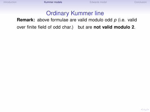
Ordinary Kummer lineRemark: above formulae are valid modulo odd p (i.e. valid

over finite field of odd char.) but are not valid modulo 2.

Introduction Kummer models Edwards model Conclusion

Ordinary Kummer lineRemark: above formulae are valid modulo odd p (i.e. valid

over finite field of odd char.) but are not valid modulo 2.

Solution: [Gau.&Lub. 08]

1. Choose an ordinary elliptic curve over F2m ;

2. Lift it over Z2m (so we can use 2−adic valuation);

3. Change of variables (old theta (x , y)⇒ new theta (X ,Y ));

4. Compute formulae using new theta functions;

5. Reduce modulo 2.

Introduction Kummer models Edwards model Conclusion

Ordinary Kummer line

Valid formulae for ordinary Kummer line over F2m .

PseudoAdd(P1,P2,R)

In: Pi = [Xi : Yi ] and R = P1 − P2

Out: P3 = P1 + P2 := [X : Y ]

1. X = (X1X2 + Y1Y2)2/X3;

2. Y = (X1Y2 + X2Y1)2/Y3;

Complexity: 3M + 2S + 1m

Double(P1)

In: P = [X1 : Y1]

Out: 2P = [X : Y ].

1. X = (X 21 + Y 2

1 )2;

2. Y = (X1Y1)2/b;

Complexity: 1M + 3S + 1m

Here

– b is new theta constant.

Introduction Kummer models Edwards model Conclusion

Kummer line for supersingular elliptic curve

Introduction Kummer models Edwards model Conclusion

Supersingular Kummer line

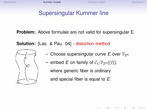
Problem: Above formulae are not valid for supersingular E.

Solution: [Las. & Pau. 04] - distortion method

– Choose supersingular curve E over F2m

– embed E on family of Ct/F2m((t)),

where generic fiber is ordinary

and special fiber is equal to E .

Introduction Kummer models Edwards model Conclusion

Supersingular Kummer line

Let E/F2m : V 2 + a3V = U3 + a4U + a6 be supersingular;

and let Ct : V 2 + tnUV + a3V = U3 + a4U + a6 for n ∈ N.

We have C0 := E is supersingular and Ct is ordinary iff t 6= 0.

Introduction Kummer models Edwards model Conclusion

Supersingular Kummer line

Let E/F2m : V 2 + a3V = U3 + a4U + a6 be supersingular;

PseudoAdd(Q1,Q2,R)

In: Qi = [Ui : Zi ] and R = Q1 −Q2

Out: Q3 = Q1 + Q2 := [U : Z ]

1. Z = (U1Z2 + U2Z1)2/Z3;

2. U = (a43Z 2

1 Z 22 + U3Z )/Z3.

Complexity: 4M + 1S + 1m

Double(Q1)

In: Q = [U1 : Z1]

Out: 2Q = [U : Z ].

1. Z = a43Z 4

1 ;

2. U = U41 + a4

4Z 41 .

Complexity: 4S + 2m

Application:

– We can compute pairings

Introduction Kummer models Edwards model Conclusion

Example of Weil pairing computation

F25 := F2[x ]/(x5 + x2 + 1). Let α root of x5 + x2 + 1.

Let E : y2 + α5y = x3 + α23x + 1 be supersingular curve.

We have #E(F25) = 25, choose ` = 5 and embed. degree d = 4.

So, we choose F(25)4 := F25 [x ]/(x4 + αx3 + α15x2 + α6x + α)

P := (α13, α6) ∈ E [`](F25) and Q := (β967372, β791798) ∈ E [`](F(25)4)

where β is the root of x4 + αx3 + α15x2 + α6x + α

We compute P + Q := (β638382, β116583) ∈ E [`](F(25)4)

Introduction Kummer models Edwards model Conclusion

Example of Weil pairing computation

We use [Rob&Lub] algorithm:

O P 2P · · · `P = λ0P · O

Q P ⊕ Q 2P ⊕ Q · · · `P ⊕ Q = λ1P · O

2Q P ⊕ 2Q...

...

`Q = λ0Q · O P ⊕ `Q = λ1

Q · P

and find Weil pairing

w(P,Q) =λ1

Q

λ0Q·λ0

P

λ1P:=

α17

β878005 ·β416202

β614001 := β419430 2

Introduction Kummer models Edwards model Conclusion

Binary Edwards models

• Ordinary Edwards model over characteristic two

• Supersingular Edwards model over characteristic two.

Introduction Kummer models Edwards model Conclusion

Edwards model

Let a ∈ C∗, an Edwards model of elliptic curve is:

E : x2 + y2 = a2(1 + x2y2).

The corresponding Weierstrass model is

C : z2 = (x2 − a2)(x2 − 1/a2);

The corresponding level 4 Theta model is of form:{a2

00X 20 = a2

01X 21 + a2

10X 22

a200X 2

3 = a210X 2

1 − a201X 2

2

⇔

{Z 2

0 + Z 22 = 2λZ1Z3

Z 21 + Z 2

3 = 2λZ0Z2

Introduction Kummer models Edwards model Conclusion

Edwards model

Let a ∈ C∗, an Edwards model of elliptic curve is:

E : x2 + y2 = a2(1 + x2y2).

Addition: Pi = (xi ; yi) on E , the sum P3 = P1 + P2 is give by:

x3 =1a· x1y2 + x2y1

1 + x1x2y1y2y3 =

1a· y1y2 − x1x2

1− x1x2y1y2

Complexity: 4M + 2I + 2m (using Montgomerry ladder)

Remark:

• The additive formulae are valid when P1 := P2.

• Addition law can be describe geometrically [A. 08].

Introduction Kummer models Edwards model Conclusion

Edwards model1. C the unic conic pass through ∞1 := [1 : 0 : 0],

∞2 := [0 : 1 : 0], O := (0,1),P1 and P2.

2. C intersect Edwards curve E at unic other point P

3. The symmetric of P give the point P3.

Introduction Kummer models Edwards model Conclusion

Binary ordinary Edwards modelRemark: Edwards model is valid over odd field, but is singular

curve over characteristic 2 field.

Introduction Kummer models Edwards model Conclusion

Binary ordinary Edwards modelRemark: Edwards model is valid over odd field, but is singular

curve over characteristic 2 field.Solution: [D. 10]

1. Choose an ordinary elliptic curve over F2m ;

2. Lift it over Z2m (so we can use 2−adic valuation);

3. Change of theta (old (Xi)1<=i<=4 ⇒ new (Zi)1<=i<=4)

4. Compute formulae using new theta functions;

5. Reduce modulo 2.

Introduction Kummer models Edwards model Conclusion

Binary ordinary Edwards modelThe binary (ordinary) Edwards model over k is of form:

Ec : x2 + y2 + cxy = 1 + x2y2, with c ∈ k∗.

The corresponding Weierstrass model is

C : z2 + tz = t3 + 1/c4;

The corresponding level 4 theta model is:{Z 2

0 + Z 22 = λZ1Z3

Z 21 + Z 2

3 = λZ0Z2, where λ2 = c.

Introduction Kummer models Edwards model Conclusion

Binary ordinary Edwards modelThe binary (ordinary) Edwards model over k is of form:

Ec : x2 + y2 + cxy = 1 + x2y2, with c ∈ k∗.

Addition: Pi = (xi ; yi) on Ec , the sum P3 = P1 + P2 is give by:

x3 =(x1 + x2)(1 + y1y2)

(y1 + y2)(1 + x1x2)and y3 =

x1x2 + y1y2

1 + x1x2y1y2.

Complexity: 5M + 2I

Remark: We can describe the addition law geometrically.

Introduction Kummer models Edwards model Conclusion

Conclusion• Use two methods to tackle problems of characteristic 2;

• Have efficient formulae for Kummer line (⇒ pairings);

• Have a supersingular Edwards model but addition law is slow;

Introduction Kummer models Edwards model Conclusion

Conclusion• Use two methods to tackle problems of characteristic 2;

• Have efficient formulae for Kummer line (⇒ pairings);

• Have a supersingular Edwards model but addition law is slow;

• We need to efficient the addition law on supersingular Edwards.

• What about genus 2 Edwards models?

Introduction Kummer models Edwards model Conclusion

References

Bernstein D.J., Lange T., and Farashahi R.R.Binary Edwards curves.Cryptology ePrint Archive, 2008/171

Carls R.,Theta null points of 2-adic canonical liftsPreprint is available at arXiv 2005

Edwards H. M.A normal form for elliptic curvesBulletin of the American Mathematical Society 44(2007)

Gaudry P.,Fast genus 2 arithmetic based on Theta functions.Journal of Mathematical Cryptology. pp. 243-265. 2007.

Gaudry P. and Lubicz D.The arithmetic of characteristic 2 Kummer surfaces and of elliptic Kummer lines.Finite Fields and Their Applications, 2009.

Laszlo Y. and Pauly C.,The Frobenius map, rank 2 vector bundles and Kummer ′s quartic surface in characteristic 2 and 3.Advances Mathematics. pp 185(2):246–269, 2004.

Mumford D.,Tata lectures on theta I et II, volume 43 of Progress in Mathematics.Birkhäuser Boston Inc., Boston, MA, 1984.