krls: A Stata Package for Kernel-Based Regularized Least ...jhain/Paper/JSS2015_RR.pdf · 2 krls: A...

JSS Journal of Statistical Software, Volume , Issue . http://www.jstatsoft.org/

krls: A Stata Package for

Kernel-Based Regularized Least Squares

Jeremy FerwerdaMassachusetts Institute of Technology

Jens HainmuellerStanford University

Chad J. HazlettUniversity of California Los Angeles

Abstract

The Stata package krls implements kernel-based regularized least squares (KRLS), amachine learning method described in Hainmueller and Hazlett (2014) that allows users totackle regression and classification problems without strong functional form assumptionsor a specification search. The flexible KRLS estimator learns the functional form fromthe data, thereby protecting inferences against misspecification bias. Yet it neverthelessallows for interpretability and inference in ways similar to ordinary regression models. Inparticular, KRLS provides closed-form estimates for the predicted values, variances, andthe pointwise partial derivatives that characterize the marginal effects of each independentvariable at each data point in the covariate space. The method is thus a convenient andpowerful alternative to OLS and other GLMs for regression-based analyses. We alsoprovide a companion package and replication code that implements the method in R.

Keywords: machine learning, regression, classification, prediction, Stata, R.

1. Overview

GLMs remain the workhorse modeling technology for most regression and classification prob-lems in social science research. GLMs are relatively easy to use and interpret, and allow avariety of outcome variable types with different assumed conditional distributions. However,by using the data in a linear way within the appropriate link function, all GLMs impose strin-gent functional form assumptions that are often potentially inaccurate for social science data.For example, linear regression typically requires that the marginal effect of each covariate isconstant across the covariate space. Similarly, logistic regression assumes that the log-odds

http://www.jstatsoft.org/

2 krls: A Stata Package for Kernel-Based Regularized Least Squares

(that the outcome equals one) are linear in the covariates. Such constant marginal effectassumptions can be dubious in the social world, where marginal effects are often expected tobe heterogenous across units and levels of other covariates.

It is well-known that misspecification of models leads not only to an invalid estimate of howwell the covariates explain the outcome variable, but may also lead to incorrect inferencesabout the effects of each covariate (see e.g., Larson and Bancroft 1963; Ramsey 1969; White1981; Hardie and Linton 1994; Sekhon 2009). In fact, for parametric models, leaving out animportant function of an observed covariate can result in the same type of omitted variablebias as failing to include an important unobserved confounding variable. The conventionalapproach to dealing with this risk is for the user to attempt to add additional terms (e.g.,a squared term, interaction, etc.) that can account for specific forms of interactions andnonlinearities. However “guessing” the correct functional form is often difficult. Moreover,including these higher-order terms can actually worsen the problem and lead investigatorsto make incorrect inferences due to misspecification (see Hainmueller and Hazlett 2014). Inaddition, results may be highly model dependent, with slight modifications to the functionalform changing estimates radically (e.g., King and Zeng 2006; Ho, Imai, King, and Stuart2007).

Presumably, social scientists are aware of these problems but commonly resort to GLMsbecause they lack convenient alternatives that would allow them to easily relax the functionalform assumptions while maintaining a high degree of interpretability. While more flexiblemethods, such as neural networks (e.g., Beck, King, and Zeng 2000a) or generalized additivemodels (GAMs, e.g., Hastie and Tibshirani 1990; Beck and Jackman 1998; Wood 2004) haveoccasionally been proposed, they have not received widespread usage by social scientists, mostlikely because they lack the ease of use and interpretation that GLMs afford.

This paper introduces a Stata (StataCorp 2015) package called krls which implements kernel-based regularized least squares (KRLS), a machine learning method described in Hainmuellerand Hazlett (2014) that allows users to tackle regression and classification problems withoutmanual specification search and strong functional form assumptions. To our knowledge, Statacurrently offers no packaged routines to implement machine learning methods like KRLS.1

One important contribution of this article therefore is to close this gap by providing Statausers with a routine to implement the KRLS method and thus to benefit from advances inmachine learning. In addition, we also provide a package called KRLS that implements thesame methods in R (R Core Team 2014). While the focus of this article is on the Statapackage, below we also briefly discuss the R version and provide companion replication codethat implements all examples in both Stata and R.

KRLS was designed to allow investigators to move beyond GLMs for classification and re-gression problems, while retaining their ease-of-use and interpretability. The KRLS estimatoroperates in a much larger space of possible functions based on the idea that observations withsimilar covariate values are expected to have similar outcomes on average.2 Furthermore,KRLS employs regularization which amounts to a prior preference for smoother functions

1One exception is the gam command by Royston and Ambler (1998), which provides a Stata interface toa version of the Fortran program gamfit for the GAM model written by Trevor Hastie and Robert Tibshirani(Hastie and Tibshirani 1990).

2This notion that similar observations should having similar outcomes is also a motivation for methodssuch as smoothers and k-nearest neighbors models. However, while those other methods are “local” and thussusceptible to the curse of dimensionality, KRLS retains the characteristics of a “global” estimator, i.e., theestimate at a given point may depend to some degree on any other observation in the dataset. Accordingly, it

Journal of Statistical Software 3

over erratic ones. This allows KRLS to minimize over-fitting, reducing the variance andfragility of estimates, and diminishing the influence of “bad leverage” points. As explainedin Hainmueller and Hazlett (2014), the regularization also helps to recover efficiency so thatKRLS is typically not much less efficient than OLS even if the data are truly linear. KRLS ap-plies most naturally to continuous outcomes, but also works well with binary outcomes. Themethod has been shown to have comparable or superior performance to many other machinelearning approaches for both (continuous) regression and (binary) classification tasks, suchas k-nearest neighbors, support vector machines, neural networks, and generalized additivemodels (Rifkin, Yeo, and Poggio 2003; Zhang and Peng 2004; Hainmueller and Hazlett 2014).

Central to its useability, the KRLS approach produces interpretable results similar to thetraditional output of GLMs, while allowing richer interpretations if desired. In addition, itallows closed-form solutions for many quantities of interest. Finally, as shown in Hainmuellerand Hazlett (2014), the KRLS estimator has desirable statistical properties, including un-biasedness, consistency, and asymptotic normality under mild regularity conditions. Givenits combination of flexibility and interpretability, KRLS can be used for a wide variety ofmodeling tasks. It is suitable for modeling problems whenever the correct functional form isnot known, including exploratory analysis, model-based causal inference, prediction problems,propensity score estimation, or other regression and or classification problems.

The krls package is distributed through the Statistical Software Components (SSC) archiveprovided at http://ideas.repec.org/c/boc/bocode/s457704.html.3 The key commandin the krls package is krls which functions much like Stata’s reg command and fits a KRLSmodel where the outcome variable is regressed on a set of covariates. Following this modelfit, a second function, predict, can be used to predict fitted values, residuals, and otherquantities just like with other Stata estimation commands. We illustrate the use of thisfunction with example data originally used in Beck, Levine, and Loayza (2000b). This datafile, growthdata.dta, “ships” with the krls package.

2. Understanding kernel-based regularized least squares

The approach underlying KRLS has been well established in machine learning since the 1990sunder a host of names including regularized least squares (e.g., Rifkin et al. 2003), regular-ization networks (e.g., Evgeniou, Pontil, and Poggio 2000), and kernel ridge regression (e.g.,Saunders, Gammerman, and Vovk 1998, Cawley and Talbot 2002).4

Hainmueller and Hazlett (2014) provide a detailed explanation of the KRLS methodology andestablish its statistical properties together with simulations and real-data examples. Here wefocus on how users can implement this approach through the krls package. We thus provideonly a brief review of the theoretical background.

We first set notation and key definitions. Assume that we draw i.i.d. data of the form (yi, xi),where i = 1, ..., N indexes the observations, yi ∈ R is the outcome of interest, and xi isa 1 × D real-valued vector xi in RD, taken to be our vector of covariate values. For ourpurposes, a kernel is defined as a (symmetric and positive semi-definite) function of two input

is more resistant to the curse of dimensionality and can be used in data with hundreds or even thousands ofdimensions.

3We thank the editor Christopher F. Baum for managing the SSC archive.4The method discussed here may also be considered a (Gaussian) radial basis function (RBF) neural network

with weight decay and is also closely related to Gaussian process regression (Wahba 1990; Rasmussen 2003).

http://ideas.repec.org/c/boc/bocode/s457704.html


patterns, k(xi, xj), mapping onto a real-valued output.5,6 For our purpose, kernel functionscan be treated as providing a measure of similarity between the covariate vectors of twoobservations. Here we use the Gaussian kernel, defined as

k(xj , xi) = e−‖xj−xi‖

2

σ2 , (1)

where ‖xj−xi‖ is the Euclidean distance between the covariate vectors xj and xi and σ2 ∈ R+

is the bandwidth of the kernel function. This kernel function evaluates to its maximum valueof one only when the covariate vectors xj and xi are identical, and approaches zero as xj andxi grow far apart.

As examined in Hainmueller and Hazlett (2014), KRLS can be understood through severalperspectives. Here we limit discussion to the viewpoint we believe is most valuable for thosewithout prior experience in kernel methods, the “similarity-based view” in which the KRLSmethod can be thought of in two stages. First, it fits functions using kernels, based on thepresumption that there is useful information embedded in how similar a given observation isto other observations in the dataset. Second, it utilizes regularization, which gives preferenceto simpler functions. We describe both stages below.

2.1. Fitting with kernels

We begin by assuming that the target function y = f(x) can be well approximated by somefunction in the space of functions represented by

f(x) =N∑i=1

cik(x, xi) (2)

where k(x, xi) measures the similarity between our point of interest (x) and one of N covariatevectors xi, and ci is a weight for each covariate vector. Functions of this type leverageinformation about the similarity between observations. Imagine we have some test-point x?

at which we would like to evaluate the function value, and suppose that the covariate vectorsxi and their weights ci have all been fixed. For such a test point, the predicted value is givenby

f(x?) = c1k(x?, x1) + c2k(x?, x2) + . . .+ cNk(x?, xN ).

Since k(x?, xj) is a measure of the similarity between x? and xj , we see that the value ofk(x?, xj) will grow larger as we move the test-point x? closer to xj . In other words, thepredicted outcome at the test point is given by a weighted sum of how similar the test pointis to each observation in the (training) data set. The equation can thus be thought of as

f(x?) = c1(similarity of x? to x1) + c2(sim. of x? to x2) + . . .+ cN (sim. of x? to xN ).

Introducing a matrix notation helps to illustrate the underlying operations. Let matrix K bethe N ×N symmetric kernel matrix whose jth, ith entry is k(xj , xi); it measures the pairwise

5The use of kernels for regression in our context should not be confused with non-parametric methodscommonly called “kernel regression” that involve using a kernel to construct a weighted local estimate (Fanand Gijbels 1996; Li and Racine 2007).

6By positive semi-definite, we mean that∑i

∑j αiαjk(xi, xj) ≥ 0, ∀αi, αj ∈ R, x ∈ RD, D ∈ Z+.


similarities between each of the N covariate vectors xi. Let c = [c1, ..., cN ]> be the N × 1vector of choice coefficients and y = [y1, ..., yN ]> be the N × 1 vector of outcome values.Equation 2 as applied to each observed x in the observed data or training set can then berewritten in vector form as:

y = Kc =

k(x1, x1) k(x1, x2) . . . k(x1, xN )

k(x2, x1). . .

...k(xN , x1) k(xN , xN )

c1c2

cN

. (3)

In this form we see KRLS as a linear system in which we estimate y? for any x? as a lin-ear combination of basis functions, each of which is a measure of x?’s similarity to otherobservations in the (training) data set.

2.2. Regularization

While this approach re-expresses the data in terms of new basis functions, it effectively solvesfor N parameters using N observations. A perfect fit could be sought by choosing c =K−1y, but even when K is invertible, such a fit would be highly unstable and lacking ingeneralizability. To make use of the information in the columns of K, we impose an additionalassumption: that we prefer smoother, less complicated functions. We thus employ Tikhonovregularization (Tychonoff 1963), solving an optimization problem over both empirical fit andmodel complexity given by choosing

argminf∈H

∑i

(V (yi, f(xi))) + λR(f) (4)

where V (yi, f(xi)) is a loss function that computes how “wrong” the function is at eachobservation, H is a hypothesis space of possible functions, R is a “regularizer” measuring the“complexity” of function f , and λ ∈ R+ is a parameter that determines the tradeoff betweenmodel fit and complexity. Larger values of λ result in a larger penalty for the complexity ofthe function thus placing a higher premium on model parsimony; lower values of λ will havethe opposite effect of placing a higher premium on model fit.

For KRLS, we choose V to be squared loss, and we choose the regularizer R to be the squareof the L2 norm,7 〈f, f〉H = ||f ||2K . For the Gaussian kernel, this choice of norm imposes anincreasingly high penalty on “wiggly” or higher-frequency components of f . Moreover, thisnorm can be computed as ||f ||2K =

∑i

∑j cicjk(xi, xj) = c>Kc (Scholkopf and Smola 2002).

Finally, the hypothesis space H is the space of functions described above, y = Kc. Theresulting Tikhonov problem is

c? = argminc∈RD

(y −Kc)>(y −Kc) + λc>Kc. (5)

Accordingly, y? = Kc? provides the best fitting approximation. For a fixed choice of λ,since this fit is a least-squares fit, it can be interpreted as providing the best approximation

7To be precise, this the L2 norm in the Reproducing Kernel Hilbert Space of functions defined by our choiceof kernel.


to the conditional expectation function, E[y|X,λ]. Notice that this minimization is almostequivalent to a ridge regression in a new set of features, one which measures the similarity ofa covariate vector to each of the other covariate vectors.8

Finally, we can solve for the solution by differentiating the objective function with respectto the choice coefficients c and solving the resulting first order conditions, arriving at theclosed-form solution

c? = (K + λI)−1y. (6)

3. Numerical implementation

One key advantage of KRLS is that we have a closed-form solution for the estimator of thechoice coefficients that provides the solution to the Tikhonov regularization problem withinour flexible space of functions. This estimator, as described in Equation 6, is numericallyattractive. We need to build the kernel matrix K by computing all pairwise distances andthen add λ to the diagonal. The resulting matrix is symmetric, positive definitive, and well-conditioned (for large enough λ) so inverting it is straightforward. The only caveat here isthat creating the (N ×N) kernel matrix can be memory intensive in very large data sets.

3.1. Data processing and choice of parameters

Before examining the choice of λ and σ2, it is important to note that krls always standardizesvariables prior to analysis by subtracting off the sample means and dividing by the samplestandard deviations.9

First, we must chose the regularization parameter λ. The default in the krls function is touse a standard cross-validation technique, choosing the value of λ that minimizes the sumof the squared leave-one-out errors. In other words, we find the λ that optimizes how wella model that is fitted on all but one observation predicts the left-out observation. For anychoice of λ, N different leave-one-out predictions can be made. The sum of squared errorsover these gives the leave-one-out error (LOOE). One nice numerical feature of this approachis that the LOOE can be efficiently computed in O(N1) time for any valid choice of λ usingthe formula LOOE = c

diag(G−1)where G = K+λI (see Rifkin and Lippert 2007). Notice that

the krls function also provides the lambda() option which users can use to supply a desiredvalue of λ and this feature can be used to implement more complicated approaches if needed.

Second, we also must choose the kernel bandwidth σ2. In the context of KRLS this is princi-pally a measurement decision incorporated into the kernel definition that governs how distanttwo covariate vectors xi and xj can be from each other and still be considered relatively

8A conventional ridge regression using the columns of K as predictors would use the norm ||f ||2 = 〈c, c〉,while we use the norm ||f ||2K = c>Kc, corresponding to a space of functions induced by the kernel. This ismore fully explained in Hainmueller and Hazlett (2014).

9De-meaning the data (or otherwise accounting for an intercept) is important in regularized methods: thefunctions f(x) and f(x) + b for constant b do not in general have the same norm, and thus will be penalizeddifferently by regularization. Since this is generally undesirable, we simply remove additive constants by de-meaning the data. Normalizing the data to have a variance of one for each covariate is commonly used inpenalized methods such as KRLS to ensures that the model is invariant to unit-of-measure decisions on anyof the covariates. All estimates are subsequently returned to the original scale and location so this re-scalingdoes not affect the generalizability or interpretation.


similar.10 Accordingly, for KRLS our objective is to chose σ2 such that the columns of Kextract useful information from X. A reasonable requirement for social science data is that atleast some observations can be considered similar to each other, some are different from eachother, and many fall in-between. As explained in Hainmueller and Hazlett (2014), a reliablechoice to satisfy this prior is to set σ2 = D, where D = dim(X). A theoretical justificationfor this default choice is that for standardized data the average (Euclidean) distance betweentwo observations that enters into the kernel calculation, E[||xj − xi||2], is equal to 2D. Thechoice of σ2 = 1D typically produces a reasonable empirical distribution of the values in K.The krls command also provides a sigma() that allows the user to apply her own value forσ2 if needed.

3.2. Interpretation and quantities of interest

One important benefit of KRLS over many other flexible modeling approaches is that thefitted KRLS model lends itself to a range of interpretational tools. Below we briefly discussthe quantities of interest that users may wish to extract and make inferences about from fittedmodels.

Estimating E[y|X] and first differences

KRLS provides an estimate of the conditional expectation function that describes how theaverage of y varies across levels of X = x. This allows the routine to produce fitted valuesor out-of-sample predictions. Other quantities of interest such as first differences can also becomputed. For example, to estimate the average treatment effect of a binary variable, W , wecan simply create two datasets that are identical to the original X, but in the first set W to onefor all observations and in the second set W to zero. We can then compute the first differenceusing 1

N

∑i[y|W = 1, X]− 1

N

∑i[y|W = 0, X] as our estimate of the average marginal effect.

Of course, the covariates can be set to other values such as the sample means, medians, etc.The krls command automatically computes and reports average first differences of this typewhen covariates are binary, with closed-form estimates of standard errors.

Partial derivatives

KRLS also provides a closed-form estimator for the pointwise partial derivatives of y with re-spect to any particular covariate. Let x(d) be a particular variable, such thatX = [x1 . . . x(d) . . . xD].Then for a single observation, j, the partial derivative of y with respect to variable d can beestimated by

∂y

∂x(d)j

=−2

σ2

∑i

cie−||xi−xj ||

2

σ2 (x(d)i − x

(d)j ) (7)

Estimating the partial derivatives allows researchers to explore the pointwise marginal effects

10Note that this differs from the role of the kernel bandwidth in traditional kernel regression or kernel densityestimation where the bandwidth is typically the only smoothing parameter used for fitting. In KRLS the kernelis simply used to form K and then fitting occurs through the choice of c and a complexity penalty that isgoverned by λ. The resulting fit is thus expected to be less dependent on the exact choice of σ2 than is trueof those kernel methods in which the bandwidth is the only parameter. Moreover, since there is a tradeoffbetween σ2 and λ (increasing either can increase smoothness), a range of σ2 values is typically acceptable andleads to similar fits after optimizing over λ.


of each covariate and to summarize them as desired. By default, krls computes the sample-average partial derivative of y with respect to x(d) at each point in the observed dataset

1

N

N∑i

[∂y

∂x(d)j

]=−2

σ2N

∑j

∑i

cie−||xi−xj ||

2

σ2 (x(d)i − x

(d)j ). (8)

These average marginal effects are reported in an output table that may be interpreted ina manner similar to a regression table produced by reg or other GLM commands. Theseare convenient to examine as they are somewhat analogous to the β coefficients in a linearmodel. However, it is important to remember that the underlying KRLS model now alsocaptures non-linear relationships, and the sample average pointwise marginal effects provideonly a summary. For example, a covariate could have a positive marginal effect on one areaof the covariate space and a negative effect in the other, but the average marginal effect maybe near zero. To this end, KRLS allows for interpretation beyond these average values. Inparticular, krls provides users with the means to directly assess marginal effect heterogeneityand interpret interactions, as we explain in the empirical illustrations below.

4. Implementing kernel-based regularized least squares

In this section we describe how users can utilize kernel-based regularized least squares withthe krls package.

4.1. Installation

krls can be installed from the Statistical Software Components (SSC) archive by typing

ssc install krls, all replace

on the Stata command line. A dataset associated with the package, growthdata.dta, will bedownloaded to the default Stata folder when the option all is specified.

4.2. Basic syntax

The main command in the package is the krls command that fits the KRLS model. Thebasic syntax of the krls command follows the standard Stata command form

krls depvar covar [if] [in] [, options]

A dependent variable and at least one independent variable are required. Both the dependentand independent variables may be either continuous or binary. The if and in options can beused to restrict the estimation sample to subsets of the full data set in memory.

4.3. Data

We illustrate the use of krls with the growthdata.dta data set (Beck et al. 2000b) that con-tains average GDP growth rates over 1960-1995 for 65 countries and various other covariatesthat are potentially related to growth. For each country the data set measures the followingvariables:


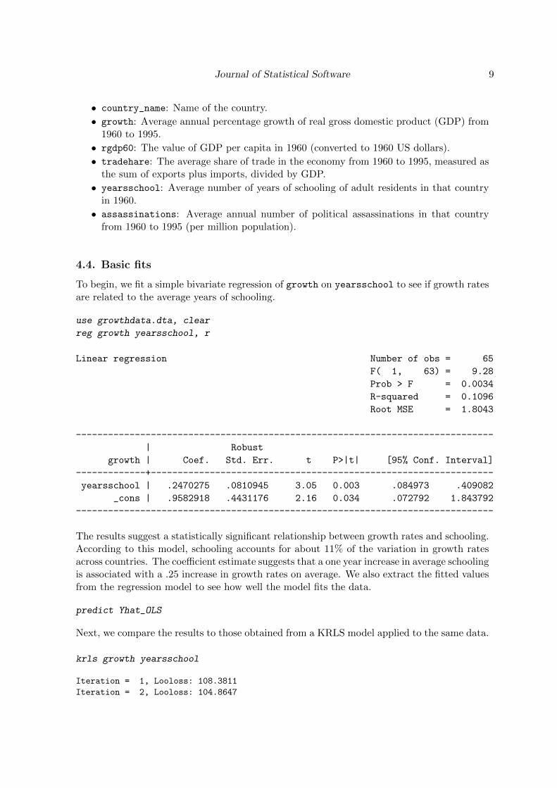
• country_name: Name of the country.

• growth: Average annual percentage growth of real gross domestic product (GDP) from1960 to 1995.

• rgdp60: The value of GDP per capita in 1960 (converted to 1960 US dollars).

• tradehare: The average share of trade in the economy from 1960 to 1995, measured asthe sum of exports plus imports, divided by GDP.

• yearsschool: Average number of years of schooling of adult residents in that countryin 1960.

• assassinations: Average annual number of political assassinations in that countryfrom 1960 to 1995 (per million population).

4.4. Basic fits

To begin, we fit a simple bivariate regression of growth on yearsschool to see if growth ratesare related to the average years of schooling.

use growthdata.dta, clear

reg growth yearsschool, r

Linear regression Number of obs = 65

F( 1, 63) = 9.28

Prob > F = 0.0034

R-squared = 0.1096

Root MSE = 1.8043

------------------------------------------------------------------------------

| Robust

growth | Coef. Std. Err. t P>|t| [95% Conf. Interval]

-------------+----------------------------------------------------------------

yearsschool | .2470275 .0810945 3.05 0.003 .084973 .409082

_cons | .9582918 .4431176 2.16 0.034 .072792 1.843792

------------------------------------------------------------------------------

The results suggest a statistically significant relationship between growth rates and schooling.According to this model, schooling accounts for about 11% of the variation in growth ratesacross countries. The coefficient estimate suggests that a one year increase in average schoolingis associated with a .25 increase in growth rates on average. We also extract the fitted valuesfrom the regression model to see how well the model fits the data.

predict Yhat_OLS

Next, we compare the results to those obtained from a KRLS model applied to the same data.

krls growth yearsschool

Iteration = 1, Looloss: 108.3811








Pointwise Derivatives Number of obs = 65

Lambda = .9855

Tolerance = .065

Sigma = 1

Eff. df = 4.879

R2 = .3191

Looloss = 94.54

growth | Avg. SE t P>|t| P25 P50 P75

-------------+--------------------------------------------------------------------

yearsschool | .336662 .076462 4.403 0.000 -.107486 .136233 .914981

-------------+--------------------------------------------------------------------

The upper left shows the iterations from the cross-validation to find the regularization pa-rameter λ that minimizes the leave-one-out error.11 The upper right reports details aboutthe sample and model fit, similar to the output of reg. The table below reports the averageof the pointwise marginal effects of schooling along with its standard error, t statistic, andp value. It also reports the 1st quartile, median, and 3rd quartile of the pointwise marginaleffects under the P25, P50, and P75 columns.

In comparison to the OLS results, the KRLS results also suggest a statistically significantrelationship between growth rates and schooling, but the average marginal effect estimate issomewhat bigger and suggests that a one year increase in schooling is associated with a .34percentage point increase in growth rates on average. Moreover, we find that the R2 fromKRLS is about three times higher and schooling now accounts for about 32% of the variationin growth rates.

Further investigation reveals that this improved model fit results because the relationshipbetween growth and schooling is not well characterized by a simple linear relationship asimplied by the OLS model above. Instead, the relationship is highly non-linear and theKRLS fit accurately learns the shape of this conditional expectation function from the data.To observe this we can use the predict function to obtain fitted values from the KRLSmodel. The predict function works much as the predict function for post model estimationin Stata, producing fitted values by default. Other options include se and residuals tocalculate standard errors of predicted values or residuals respectively.

predict Yhat_KRLS

Now we plot the fitted values to compare the model fits from the regression and the KRLSmodel. We also add to the plot the fitted values from a more flexible OLS model, Yhat_OLS2,that includes as predictors a third order polynomial of schooling.

twoway (scatter growth yearsschool, sort) ///

(line Yhat_KRLS yearsschool, sort) ///

11In the remaining examples, we show only values from the final iteration.


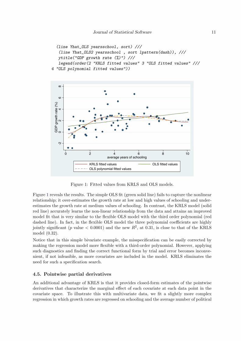
(line Yhat_OLS yearsschool, sort) ///

(line Yhat_OLS2 yearsschool , sort lpattern(dash)), ///

ytitle("GDP growth rate (%)") ///

legend(order(2 "KRLS fitted values" 3 "OLS fitted values" ///

4 "OLS polynomial fitted values"))

-20

24

68

GDP

gro

wth

rate

(%)

0 2 4 6 8 10average years of schooling

KRLS fitted values OLS fitted valuesOLS polynomial fitted values

Figure 1: Fitted values from KRLS and OLS models.

Figure 1 reveals the results. The simple OLS fit (green solid line) fails to capture the nonlinearrelationship; it over-estimates the growth rate at low and high values of schooling and under-estimates the growth rate at medium values of schooling. In contrast, the KRLS model (solidred line) accurately learns the non-linear relationship from the data and attains an improvedmodel fit that is very similar to the flexible OLS model with the third order polynomial (reddashed line). In fact, in the flexible OLS model the three polynomial coefficients are highlyjointly significant (p value < 0.0001) and the new R2, at 0.31, is close to that of the KRLSmodel (0.32).

Notice that in this simple bivariate example, the misspecification can be easily corrected bymaking the regression model more flexible with a third-order polynomial. However, applyingsuch diagnostics and finding the correct functional form by trial and error becomes inconve-nient, if not infeasible, as more covariates are included in the model. KRLS eliminates theneed for such a specification search.

4.5. Pointwise partial derivatives

An additional advantage of KRLS is that it provides closed-form estimates of the pointwisederivatives that characterize the marginal effect of each covariate at each data point in thecovariate space. To illustrate this with multivariate data, we fit a slightly more complexregression in which growth rates are regressed on schooling and the average number of political


assassinations in a country.

reg growth yearsschool assassinations , r


F( 2, 62) = 7.13

Prob > F = 0.0016

R-squared = 0.1217

Root MSE = 1.8064

--------------------------------------------------------------------------------

| Robust


---------------+----------------------------------------------------------------

yearsschool | .2366611 .0859996 2.75 0.008 .0647505 .4085718

assassinations | -.4282405 .3216043 -1.33 0.188 -1.071118 .2146374

_cons | 1.118467 .5184257 2.16 0.035 .0821487 2.154785

--------------------------------------------------------------------------------

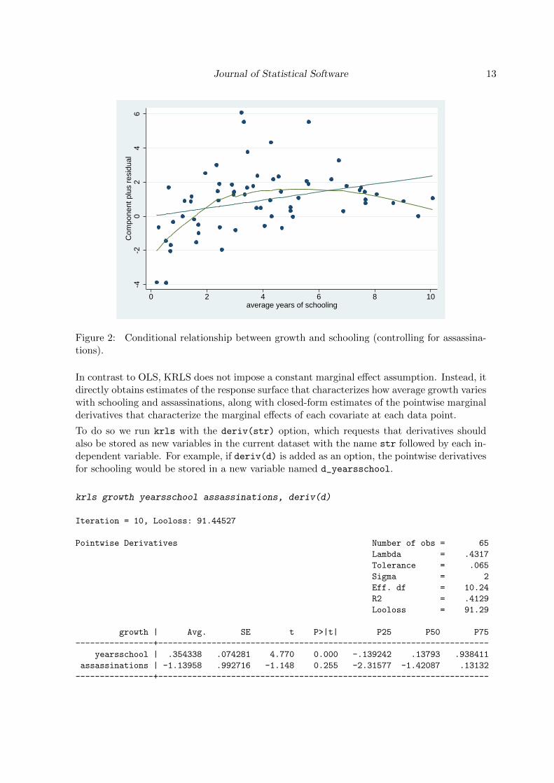
With this OLS model we find that one additional year of schooling is associated with a.24 increase in the growth rate. However, this model assumes that this marginal effect ofschooling is constant across the covariate space. To probe this assumption, we can generate acomponent-plus-residual (CR) plot to visualize the relationship between growth and schooling,controlling for the linear component of the assassinations variable. The results are shown inFigure 2. As in the first example, the regression is clearly misspecified; as indicated by thelowess line, the conditional relationship is nonlinear.

cprplot yearsschool , lowess


-4-2

02

46

Com

pone

nt p

lus

resi

dual


Figure 2: Conditional relationship between growth and schooling (controlling for assassina-tions).

In contrast to OLS, KRLS does not impose a constant marginal effect assumption. Instead, itdirectly obtains estimates of the response surface that characterizes how average growth varieswith schooling and assassinations, along with closed-form estimates of the pointwise marginalderivatives that characterize the marginal effects of each covariate at each data point.

To do so we run krls with the deriv(str) option, which requests that derivatives shouldalso be stored as new variables in the current dataset with the name str followed by each in-dependent variable. For example, if deriv(d) is added as an option, the pointwise derivativesfor schooling would be stored in a new variable named d_yearsschool.

krls growth yearsschool assassinations, deriv(d)



Lambda = .4317

Tolerance = .065

Sigma = 2

Eff. df = 10.24

R2 = .4129

Looloss = 91.29


----------------+--------------------------------------------------------------------

yearsschool | .354338 .074281 4.770 0.000 -.139242 .13793 .938411

assassinations | -1.13958 .992716 -1.148 0.255 -2.31577 -1.42087 .13132

----------------+--------------------------------------------------------------------


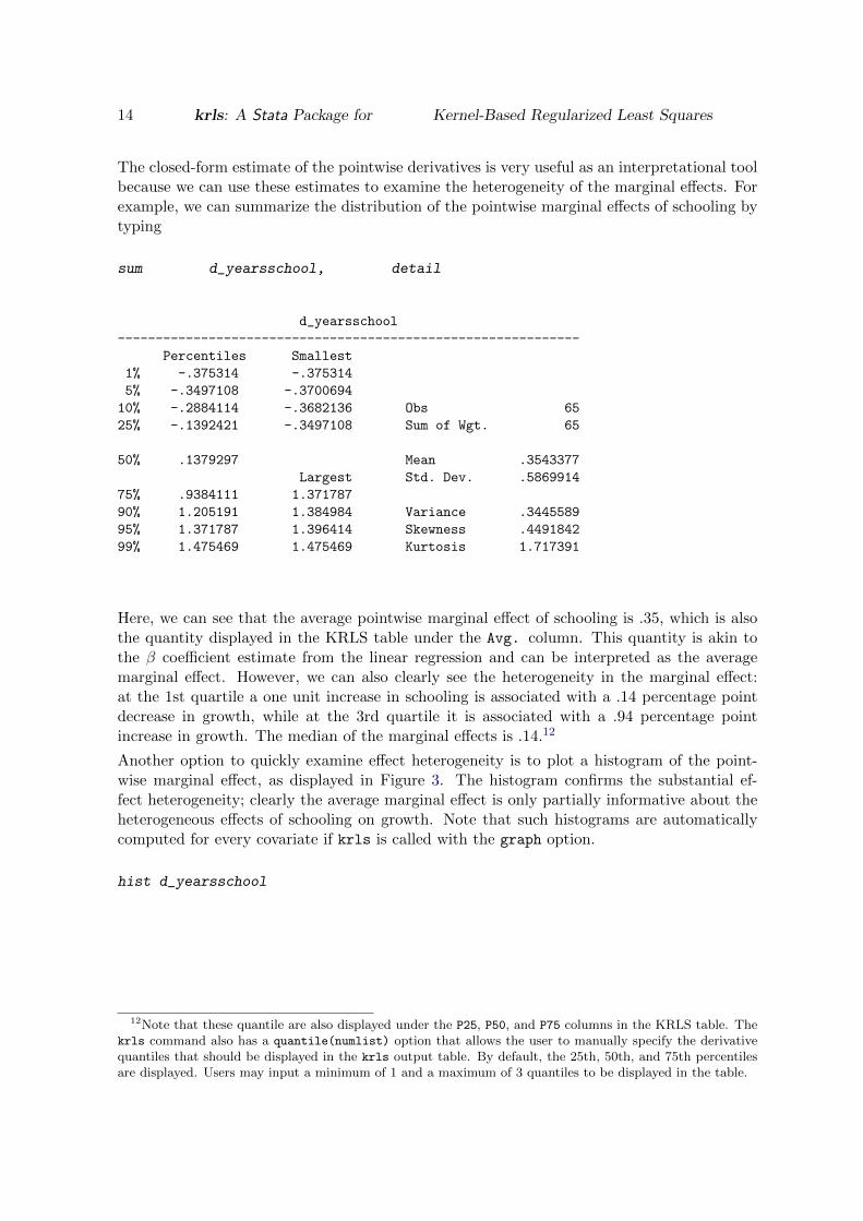
The closed-form estimate of the pointwise derivatives is very useful as an interpretational toolbecause we can use these estimates to examine the heterogeneity of the marginal effects. Forexample, we can summarize the distribution of the pointwise marginal effects of schooling bytyping

sum d_yearsschool, detail

d_yearsschool

-------------------------------------------------------------

Percentiles Smallest

1% -.375314 -.375314

5% -.3497108 -.3700694

10% -.2884114 -.3682136 Obs 65

25% -.1392421 -.3497108 Sum of Wgt. 65

50% .1379297 Mean .3543377

Largest Std. Dev. .5869914

75% .9384111 1.371787

90% 1.205191 1.384984 Variance .3445589

95% 1.371787 1.396414 Skewness .4491842

99% 1.475469 1.475469 Kurtosis 1.717391

Here, we can see that the average pointwise marginal effect of schooling is .35, which is alsothe quantity displayed in the KRLS table under the Avg. column. This quantity is akin tothe β coefficient estimate from the linear regression and can be interpreted as the averagemarginal effect. However, we can also clearly see the heterogeneity in the marginal effect:at the 1st quartile a one unit increase in schooling is associated with a .14 percentage pointdecrease in growth, while at the 3rd quartile it is associated with a .94 percentage pointincrease in growth. The median of the marginal effects is .14.12

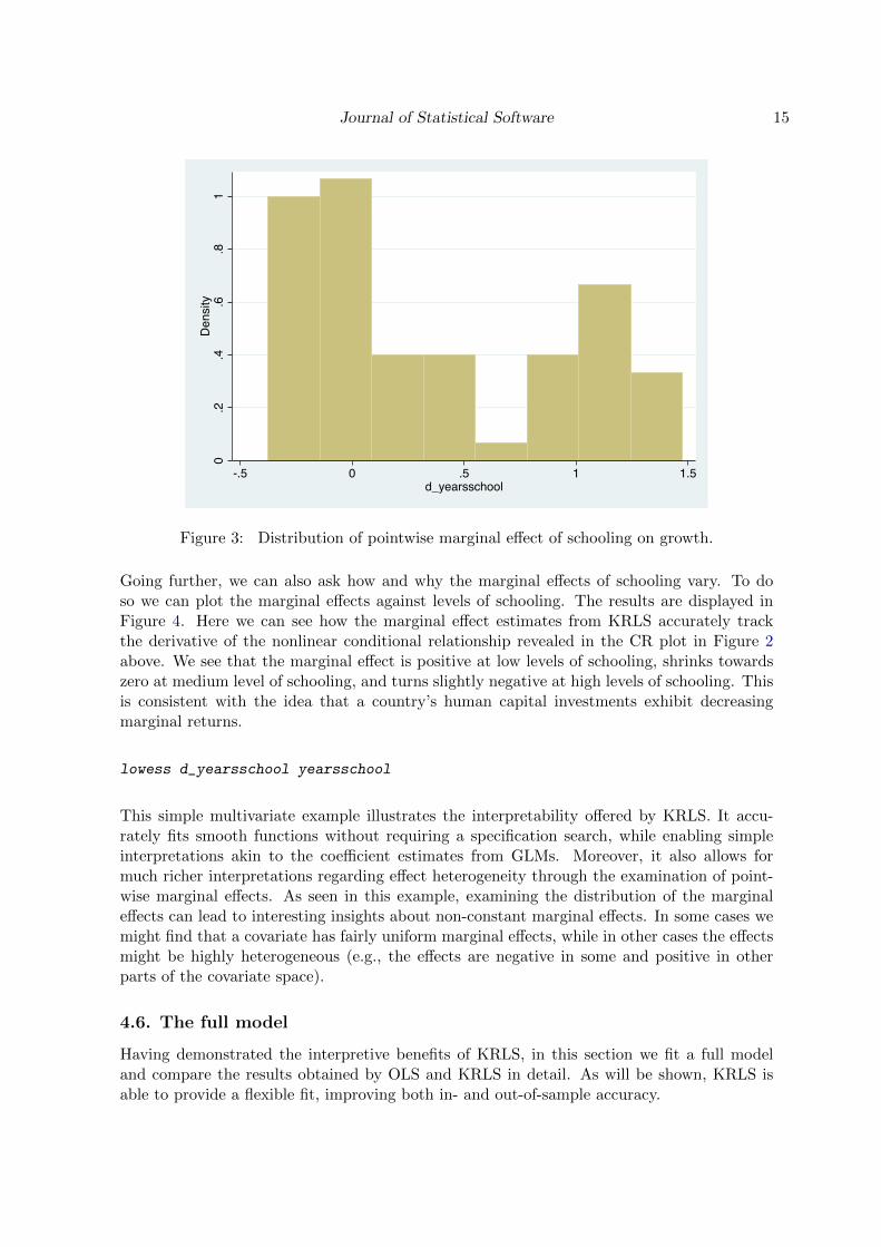
Another option to quickly examine effect heterogeneity is to plot a histogram of the point-wise marginal effect, as displayed in Figure 3. The histogram confirms the substantial ef-fect heterogeneity; clearly the average marginal effect is only partially informative about theheterogeneous effects of schooling on growth. Note that such histograms are automaticallycomputed for every covariate if krls is called with the graph option.

hist d_yearsschool

12Note that these quantile are also displayed under the P25, P50, and P75 columns in the KRLS table. Thekrls command also has a quantile(numlist) option that allows the user to manually specify the derivativequantiles that should be displayed in the krls output table. By default, the 25th, 50th, and 75th percentilesare displayed. Users may input a minimum of 1 and a maximum of 3 quantiles to be displayed in the table.


0.2

.4.6

.81

Density

-.5 0 .5 1 1.5d_yearsschool

Figure 3: Distribution of pointwise marginal effect of schooling on growth.

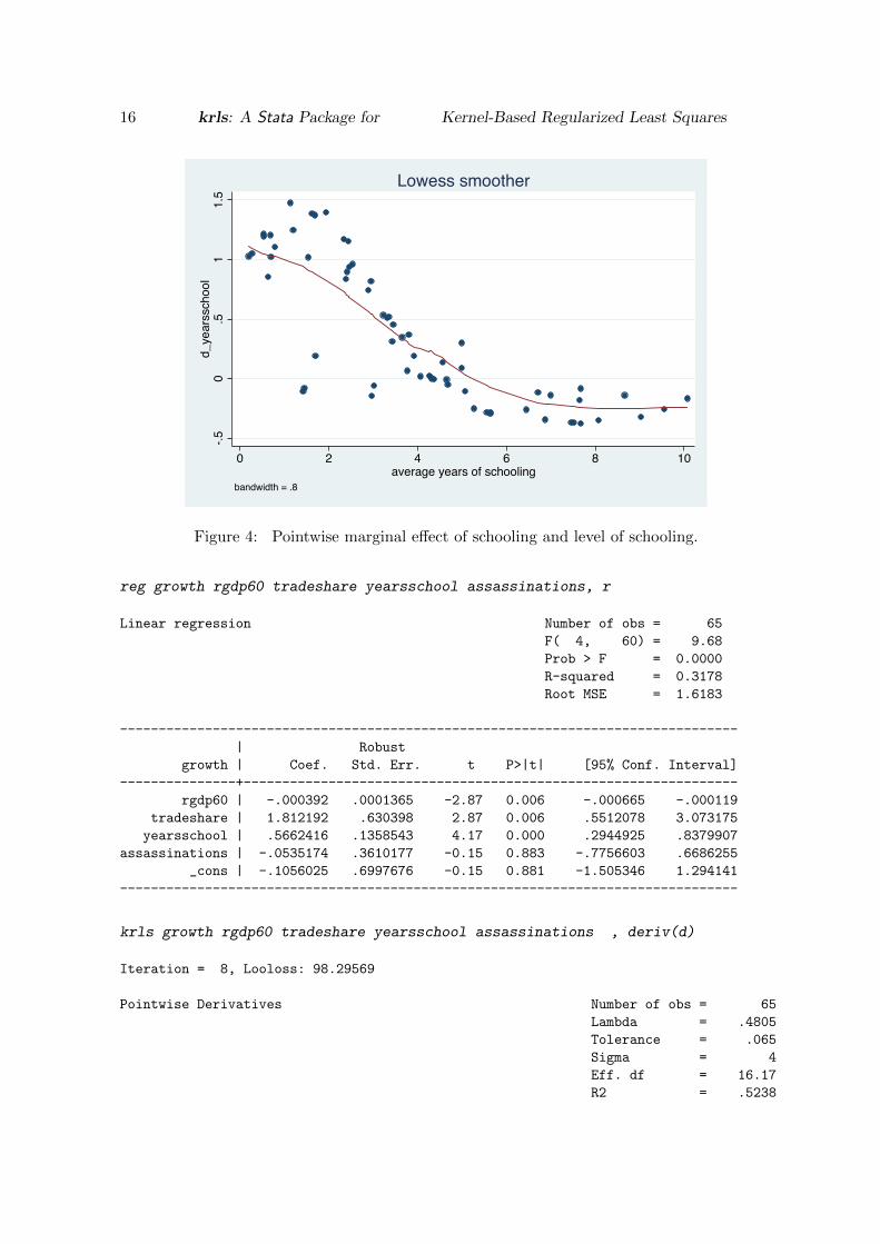
Going further, we can also ask how and why the marginal effects of schooling vary. To doso we can plot the marginal effects against levels of schooling. The results are displayed inFigure 4. Here we can see how the marginal effect estimates from KRLS accurately trackthe derivative of the nonlinear conditional relationship revealed in the CR plot in Figure 2above. We see that the marginal effect is positive at low levels of schooling, shrinks towardszero at medium level of schooling, and turns slightly negative at high levels of schooling. Thisis consistent with the idea that a country’s human capital investments exhibit decreasingmarginal returns.

lowess d_yearsschool yearsschool

This simple multivariate example illustrates the interpretability offered by KRLS. It accu-rately fits smooth functions without requiring a specification search, while enabling simpleinterpretations akin to the coefficient estimates from GLMs. Moreover, it also allows formuch richer interpretations regarding effect heterogeneity through the examination of point-wise marginal effects. As seen in this example, examining the distribution of the marginaleffects can lead to interesting insights about non-constant marginal effects. In some cases wemight find that a covariate has fairly uniform marginal effects, while in other cases the effectsmight be highly heterogeneous (e.g., the effects are negative in some and positive in otherparts of the covariate space).

4.6. The full model

Having demonstrated the interpretive benefits of KRLS, in this section we fit a full modeland compare the results obtained by OLS and KRLS in detail. As will be shown, KRLS isable to provide a flexible fit, improving both in- and out-of-sample accuracy.


-.50

.51

1.5

d_ye

arss

choo

l


bandwidth = .8

Lowess smoother

Figure 4: Pointwise marginal effect of schooling and level of schooling.

reg growth rgdp60 tradeshare yearsschool assassinations, r


F( 4, 60) = 9.68

Prob > F = 0.0000

R-squared = 0.3178

Root MSE = 1.6183

--------------------------------------------------------------------------------

| Robust


---------------+----------------------------------------------------------------

rgdp60 | -.000392 .0001365 -2.87 0.006 -.000665 -.000119

tradeshare | 1.812192 .630398 2.87 0.006 .5512078 3.073175

yearsschool | .5662416 .1358543 4.17 0.000 .2944925 .8379907

assassinations | -.0535174 .3610177 -0.15 0.883 -.7756603 .6686255

_cons | -.1056025 .6997676 -0.15 0.881 -1.505346 1.294141

--------------------------------------------------------------------------------

krls growth rgdp60 tradeshare yearsschool assassinations , deriv(d)



Lambda = .4805

Tolerance = .065

Sigma = 4

Eff. df = 16.17

R2 = .5238


Looloss = 97.5


----------------+--------------------------------------------------------------------

rgdp60 | -.000181 .000095 -1.918 0.060 -.000276 -.000206 -.000124

tradeshare | .510791 .650697 0.785 0.435 -.795706 .189738 2.04949

yearsschool | .44394 .081513 5.446 0.000 .061748 .389433 .823161

assassinations | -.899533 .589963 -1.525 0.132 -1.78801 -.872617 -.123334

----------------+--------------------------------------------------------------------

Comparing the two models, we first see that the (in-sample) R2 for KRLS is 52%, while thatof OLS is only 31%. The average marginal effects from KRLS differ from the coefficients inthe OLS model for many of the covariates. For example, the effect of trade’s share of GDPis 1.81 and significant in the OLS model, while in the KRLS models the average marginaleffect is less than a third of the size, 0.51, and highly insignificant. Moreover, while the OLSmodel suggests that assassinations have essentially no relationship with growth, the averagemarginal effect from the KRLS model is sizable: Increasing the number of assassination byone is associated with a decrease of 0.90 percentage points in growth on average.

What explains the differences in the coefficient estimates? At least part of the discrepancyis due to the previously established nonlinear relationship between schooling and growth.Accordingly, we introduce a third order polynomial for schooling to capture this nonlinearity.

reg growth rgdp60 tradeshare c.yearsschool##c.yearsschool##c.yearsschool ///

assassinations , r


F( 6, 58) = 7.80

Prob > F = 0.0000

R-squared = 0.4515

Root MSE = 1.476

----------------------------------------------------------------------------------

| Robust

growth | Coef. Std. Err. t P>|t|

------------------------------------------+---------------------------------------

rgdp60 | -.0003038 .0001372 -2.21 0.031

tradeshare | 1.436023 .6188359 2.32 0.024

yearsschool | 2.214037 .6562595 3.37 0.001

c.yearsschool#c.yearsschool | -.3138642 .1416605 -2.22 0.031

c.yearsschool#c.yearsschool#c.yearsschool | .0150468 .0088306 1.70 0.094

assassinations | -.3608613 .3457803 -1.04 0.301

_cons | -1.888819 .8992876 -2.10 0.040

----------------------------------------------------------------------------------

This improves the model fit to an R2 of 0.45 and the polynomial terms are highly jointlysignificant. But even with this improved regression model our fit is still lower than thatfrom the KRLS model, and results remain widely different for trade’s share in the economyand assassinations. To determine the source of these differences, we next examine how themarginal effects of the trade share variable depend on other variables. As a useful diagnostic,we regress the pointwise marginal effect estimates on the whole set of covariates.


reg d_tradeshare rgdp60 tradeshare yearsschool assassinations

Source | SS df MS Number of obs = 65

-------------+------------------------------ F( 4, 60) = 11.11

Model | 102.319069 4 25.5797673 Prob > F = 0.0000

Residual | 138.099021 60 2.30165035 R-squared = 0.4256

-------------+------------------------------ Adj R-squared = 0.3873

Total | 240.41809 64 3.75653266 Root MSE = 1.5171

--------------------------------------------------------------------------------

d_tradeshare | Coef. Std. Err. t P>|t| [95% Conf. Interval]

---------------+----------------------------------------------------------------

rgdp60 | .0000478 .0001369 0.35 0.728 -.0002261 .0003216

tradeshare | 2.822354 .7162343 3.94 0.000 1.389672 4.255035

yearsschool | -.2612007 .1335487 -1.96 0.055 -.5283379 .0059365

assassinations | -1.275047 .4112346 -3.10 0.003 -2.097639 -.4524557

_cons | .1635381 .5924303 0.28 0.783 -1.021499 1.348575

--------------------------------------------------------------------------------

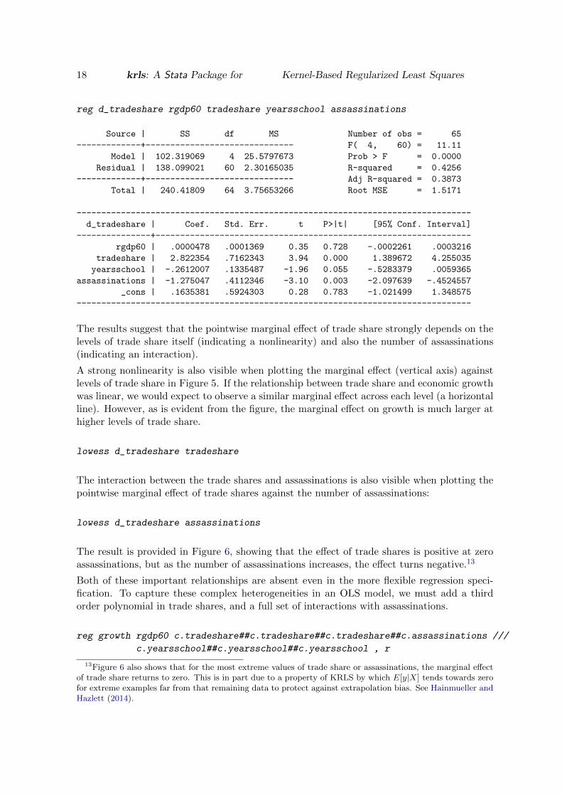
The results suggest that the pointwise marginal effect of trade share strongly depends on thelevels of trade share itself (indicating a nonlinearity) and also the number of assassinations(indicating an interaction).

A strong nonlinearity is also visible when plotting the marginal effect (vertical axis) againstlevels of trade share in Figure 5. If the relationship between trade share and economic growthwas linear, we would expect to observe a similar marginal effect across each level (a horizontalline). However, as is evident from the figure, the marginal effect on growth is much larger athigher levels of trade share.

lowess d_tradeshare tradeshare

The interaction between the trade shares and assassinations is also visible when plotting thepointwise marginal effect of trade shares against the number of assassinations:

lowess d_tradeshare assassinations

The result is provided in Figure 6, showing that the effect of trade shares is positive at zeroassassinations, but as the number of assassinations increases, the effect turns negative.13

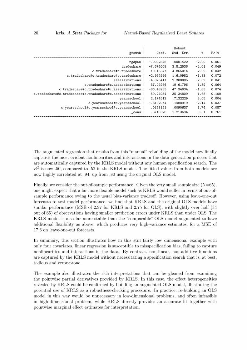
Both of these important relationships are absent even in the more flexible regression speci-fication. To capture these complex heterogeneities in an OLS model, we must add a thirdorder polynomial in trade shares, and a full set of interactions with assassinations.

reg growth rgdp60 c.tradeshare##c.tradeshare##c.tradeshare##c.assassinations ///

c.yearsschool##c.yearsschool##c.yearsschool , r

13Figure 6 also shows that for the most extreme values of trade share or assassinations, the marginal effectof trade share returns to zero. This is in part due to a property of KRLS by which E[y|X] tends towards zerofor extreme examples far from that remaining data to protect against extrapolation bias. See Hainmueller andHazlett (2014).


-4-2

02

4d_

trade

shar

e

0 .5 1 1.5 2trade share of GDP

bandwidth = .8

Lowess smoother

Figure 5: Pointwise marginal effect of trade share and level of trade share.

-4-2

02

4d_

trade

shar

e

0 .5 1 1.5 2 2.5number of assassinations

bandwidth = .8

Lowess smoother

Figure 6: Pointwise marginal effect of trade share and number of assassinations.


F( 11, 53) = 89.65

Prob > F = 0.0000

R-squared = 0.5012

Root MSE = 1.4723

------------------------------------------------------------------------------------------------


| Robust

growth | Coef. Std. Err. t P>|t|

--------------------------------------------------------+---------------------------------------

rgdp60 | -.0002845 .0001422 -2.00 0.051

tradeshare | -7.674608 3.812536 -2.01 0.049

c.tradeshare#c.tradeshare | 10.15347 4.865014 2.09 0.042

c.tradeshare#c.tradeshare#c.tradeshare | -2.954996 1.610982 -1.83 0.072

assassinations | -4.823411 2.308085 -2.09 0.041

c.tradeshare#c.assassinations | 37.04956 19.61796 1.89 0.064

c.tradeshare#c.tradeshare#c.assassinations | -86.43233 47.34634 -1.83 0.074

c.tradeshare#c.tradeshare#c.tradeshare#c.assassinations | 59.24934 35.34809 1.68 0.100 |

yearsschool | 2.174512 .7132229 3.05 0.004 |

c.yearsschool#c.yearsschool | -.3192074 .1488919 -2.14 0.037

c.yearsschool#c.yearsschool#c.yearsschool | .0158121 .0090637 1.74 0.087

_cons | .3710328 1.213694 0.31 0.761

------------------------------------------------------------------------------------------------

The augmented regression that results from this “manual” rebuilding of the model now finallycaptures the most evident nonlinearities and interactions in the data generation process thatare automatically captured by the KRLS model without any human specification search. TheR2 is now .50, compared to .52 in the KRLS model. The fitted values from both models arenow highly correlated at .94, up from .80 using the original OLS model.

Finally, we consider the out-of-sample performance. Given the very small sample size (N=65),one might expect that a far more flexible model such as KRLS would suffer in terms of out-of-sample performance owing to the usual bias-variance tradeoff. However, using leave-one-outforecasts to test model performance, we find that KRLS and the original OLS models havesimilar performance (MSE of 2.97 for KRLS and 2.75 for OLS), with slightly over half (34out of 65) of observations having smaller prediction errors under KRLS than under OLS. TheKRLS model is also far more stable than the “comparable” OLS model augmented to haveadditional flexibility as above, which produces very high-variance estimates, for a MSE of17.6 on leave-one-out forecasts.

In summary, this section illustrates how in this still fairly low dimensional example withonly four covariates, linear regression is susceptible to misspecification bias, failing to capturenonlinearities and interactions in the data. By contrast, non-linear, non-additive functionsare captured by the KRLS model without necessitating a specification search that is, at best,tedious and error-prone.

The example also illustrates the rich interpretations that can be gleaned from examiningthe pointwise partial derivatives provided by KRLS. In this case, the effect heterogeneitiesrevealed by KRLS could be confirmed by building an augmented OLS model, illustrating thepotential use of KRLS as a robustness-checking procedure. In practice, re-building an OLSmodel in this way would be unnecessary in low-dimensional problems, and often infeasiblein high-dimensional problem, while KRLS directly provides an accurate fit together withpointwise marginal effect estimates for interpretation.


5. Further issues

5.1. Binary predictors

As explained in Hainmueller and Hazlett (2014), KRLS works well with binary independentvariables. However, their effects should be interpreted using first differences (rather than thepointwise partial derivatives) to accurately capture the expected difference in the outcomewhen moving from the low to the high value of the predictor. The krls command auto-matically detects binary covariates and reports first differences rather than average marginaleffects in the output table and pointwise derivatives. Such variables are also marked with anasterisk as binary variables in the output table. To briefly illustrate this we code a binaryvariable for countries where the years of schooling is 3 years or higher and add this binaryregressor.

gen yearsschool3 = (yearsschool>3)

krls growth rgdp60 tradeshare yearsschool3 assassinations

.



Lambda = 1.908

Tolerance = .065

Sigma = 4

Eff. df = 8.831

R2 = .3736

Looloss = 104.8


----------------+--------------------------------------------------------------------

rgdp60 | -5.4e-06 .00005 -0.108 0.915 -.000106 -3.7e-06 .000122

tradeshare | .73428 .531422 1.382 0.172 -.083988 .611573 1.62604

*yearsschool3 | 1.26789 .42485 2.984 0.004 .750781 1.17464 1.8717

assassinations | -.26203 .317978 -0.824 0.413 -.660828 -.12919 .048142

----------------+--------------------------------------------------------------------

* average dy/dx is the first difference using the min and max (i.e., usually 0 to 1)

The results suggest that going from less to more than 3 years of schooling is associated with a1.27 percentage point jump in growth rates on average. As can be seen by the lower R2 (0.37,compared to 0.52), dichotomizing the continuous schooling variable results in a significantloss of information. With KRLS there is typically no reason to dichotomize variables becausethe model is flexible enough to capture nonlinearities in the underlying continuous variables.

5.2. Choosing the smoothing parameter by cross-validation

The krls command returns the number of iterations used to converge on a value for λ in theupper left panel of the function output. By default, the tolerance for the choice of λ is setsuch that a solution is reached when further changes in λ improve the proportion of variance


explained (in a leave-one-out sense) by less than 0.01%. This sensitivity level can be adjustedusing the ltolerance() option. Decreasing the sensitivity may improve execution time butmay result in the selection of a suboptimal value for lambda.

Further options for predictions

If the user is interested only in predictions, they can specify the suppress option to instructkrls not to calculate derivatives, first differences, and the output table. This significantlydecreases execution time, especially in higher dimensional examples.

In some cases the user might also be interested in obtaining uncertainty estimates for thepredicted values. These can be accomplished in KRLS because the method provides a closed-form estimator of the full variance-covariance matrix for fitted and predicted values. Followingthe model fit, users can simply use predict, se to generate a variable that contains thestandard errors for the predicted values.

The variance-covariance matrix of the coefficients is stored by default in e(Vcov_c). Usersmay also wish to obtain the full variance-covariance matrix for the fitted values for furthercomputations. To save execution time this matrix is not saved by default, but it can berequested using the vcov option of the krls command. If the model is fit with this optionspecified, the variance-covariance matrix of the fitted values is returned in e(Vcov_y). Alter-natively, the svcov(filename) option can be used to save this variance-covariance matrix toan external dataset.

Further options for extracting results

By default, krls returns the output table of pointwise derivatives and first differences inmatrix form in e(Output). Alternatively, the keep(filename) option can be used to storethe output table in a new dataset specified by filename.dta. sderiv(filename) can besimilarly used to save derivatives in a new dataset.

6. Kernel-based regularized least squares in R

For R users we have developed the KRLS package (Hainmueller and Hazlett 2015) whichimplements the same methods as in the Stata package described above. The KRLS pack-age is available for download on the Comprehensive R Archive Network (CRAN, http:

//CRAN.R-project.org/). We also provide a companion script that replicates all the ex-amples described above in the R version of the package.

Overall, the R and the Stata versions produce the same results and we see no significantadvantage in using one or the other (except that R is available as Free Software under theterms of the Free Software Foundation’s GNU General Public License). In particular, thenumerical implementation of the KRLS estimator is nearly identical across the two versions,with comparable run times and memory requirements.

The command structure is also broadly similar in both packages, although the commandsin the R version more closely follow the typical structure of R estimation commands. Inparticular, the main function in the R package is krls() which fits the KRLS model oncethe user–at a minimum–has specified the dependent and independent variables. In addition,the convenience functions summary(), plot(), and predict() are provided to summarize or

http://CRAN.R-project.org/

http://CRAN.R-project.org/


plot the results from the fitted KRLS model object and to generate predicted values (withstandard errors) for in-sample and out-of-sample predictions. For example, we can replicatethe full model described above using the following code

R> library(foreign)

R> library(KRLS)

R> growth <- read.dta("growthdata.dta")

R> covars <- c("rgdp60", "tradeshare",

"yearsschool", "assassinations")

R> k.out <- krls(y=growth$growth,

X=growth[,covars])

R> summary(k.out)

* *********************** *

Model Summary:

R2: 0.5237912

Average Marginal Effects:

Est Std. Error t value Pr(>|t|)

rgdp60 -0.0001814697 9.462225e-05 -1.9178330 5.981703e-02

tradeshare 0.5107908139 6.506968e-01 0.7849905 4.354973e-01

yearsschool 0.4439403707 8.151325e-02 5.4462354 9.729103e-07

assassinations -0.8995328084 5.899631e-01 -1.5247272 1.324954e-01

Quartiles of Marginal Effects:

25% 50% 75%

rgdp60 -0.0002764298 -0.0002057956 -0.0001242661

tradeshare -0.7957059378 0.1897375034 2.0494918408

yearsschool 0.0617481348 0.3894334721 0.8231607478

assassinations -1.7880077113 -0.8726170582 -0.1233344601

7. Conclusion

In this article we have described how to implement kernel regularized least squares using thekrls package for Stata. We also provided an implementation in R through the KRLS package(Hainmueller and Hazlett 2015).

The KRLS method allows researchers to overcome the rigid assumptions in widely used modelssuch as GLMs. KRLS fits a flexible, minimum-complexity regression surface to the data,accommodating a wide range of smooth non-linear, non-additive functions of the covariates.Because it produces closed-form estimates for both the fitted values and partial derivativesat every observation, the approach lends itself to easy interpretation. In future releases, wehope to improve upon the krls function by improving its speed (the current implementationbegins to slow with several thousand observations), by allowing for weights, and by providingoptions for heteroskedasticity-robust and cluster-robust standard errors.

We illustrate the use of the krls function by analyzing GDP growth rates over 1960-1995 for 65countries (Beck et al. 2000b). Compared to OLS implemented through reg, krls reveals non-linearities and interactions that substantially alter both the quality of fit and the inferences


drawn from the data. In this case, an OLS model could be re-built using insights from thekrls model. In general, however, use of krls obviates the need for a tedious specificationsearch which may still leave some important non-linearities and interactions undetected.

Acknowledgments

We would like to thank Yiqing Xu for helpful comments.


References

Beck N, Jackman S (1998). “Beyond Linearity by Default: Generalized Additive Models.”American Journal of Political Science, 42(2), 596–627.

Beck N, King G, Zeng L (2000a). “Improving Quantitative Studies of International Conflict:A Conjecture.” American Political Science Review, 94, 21–36.

Beck T, Levine R, Loayza N (2000b). “Finance and the Sources of Growth.” Journal ofFinancial Economics, 58(1), 261–300.

Cawley G, Talbot N (2002). “Reduced Rank Kernel Ridge Regression.” Neural ProcessingLetters, 16(3), 293–302.

Evgeniou T, Pontil M, Poggio T (2000). “Regularization Networks and Support Vector Ma-chines.” Advances in Computational Mathematics, 13(1), 1–50.

Fan J, Gijbels I (1996). Local Polynomial Modeling and Its Applications. Chapman and Hall.

Hainmueller J, Hazlett C (2014). “Kernel Regularized Least Squares: Reducing Misspecifica-tion Bias with a Flexible and Interpretable Machine Learning Approach.”Political Analysis,22(2), 143–168.

Hainmueller J, Hazlett C (2015). KRLS: Kernel-based Regularized Least Squares. R packageversion 0.3-6, URL http://CRAN.R-project.org/package=KRLS.

Hardie W, Linton O (1994). “Applied Nonparametric Methods.” Handbook of Econometrics,4, 2295–2339.

Hastie T, Tibshirani R (1990). Generalized Additive Models. Chapman & Hall, London.

Ho D, Imai K, King G, Stuart E (2007). “Matching as Nonparametric Preprocessing forReducing Model Dependence in Parametric Causal Inference.” Political Analysis, 15(3),199–236.

King G, Zeng L (2006). “The Dangers of Extreme Counterfactuals.” Political Analysis, 14,131–159.

Larson H, Bancroft T (1963). “Biases in Prediction by Regression for Certain IncompletelySpecified Models.” Biometrika, 50(3/4), 391–402.

Li Q, Racine J (2007). Nonparametric Econometrics: Theory and Practic. Princeton Univer-sity Press.

R Core Team (2014). R: A Language and Environment for Statistical Computing. R Foun-dation for Statistical Computing, Vienna, Austria. URL http://www.R-project.org/.

Ramsey J (1969). “Tests for Specification Errors in Classical Linear Least-Squares RegressionAnalysis.” Journal of the Royal Statistical Society B, 31(2), 350–371.

Rasmussen CE (2003). “Gaussian Processes in Machine Learning.” In O Bousquet, U vonLuxburg, G Ratsch (eds.), Advanced Lectures on Machine Learning, volume 3176 of LectureNotes in Computer Science, pp. 63–71. Springer-Verlag. ISBN 3-540-23122-6.

http://CRAN.R-project.org/package=KRLS

http://www.R-project.org/


Rifkin R, Yeo G, Poggio T (2003). “Regularized Least-Squares Classification.” Nato ScienceSeries Sub Series III Computer and Systems Sciences, 190, 131–154.

Rifkin RM, Lippert RA (2007). “Notes on Regularized Least Squares.” Technical report, MITComputer Science and Artificial Intelligence Laboratory.

Royston P, Ambler G (1998). “Generalized Linear Models.” Stata Technical Bulletin, 42,38–43.

Saunders C, Gammerman A, Vovk V (1998). “Ridge Regression Learning Algorithm in DualVariables.” In Proceedings of the 15th International Conference on Machine Learning.Morgan Kaufmann, San Francisco, CA.

Scholkopf B, Smola A (2002). Learning with Kernels: Support Vector Machines, Regulariza-tion, Optimization, and Beyond. The MIT Press.

Sekhon J (2009). “Opiates for the Matches: Matching Methods for Causal Inference.” AnnualReview of Political Science, 12, 487–508.

StataCorp (2015). Stata Stata Statistical Software: Release 14. StataCorp LP.

Tychonoff A (1963). “Solution of Incorrectly Formulated Problems and the RegularizationMethod.” Doklady Akademii Nauk SSSR, 151, 501–504. Translated in Soviet Mathematics,4, 1035-1038.

Wahba G (1990). Spline Models for Observational Data. Society for Industrial Mathematics.

White H (1981). “Consequences and Detection of Misspecified NonLinear Regression Models.”Journal of the American Statistical Association, 76(374), 419–433.

Wood S (2004). “Stable and Efficient Multiple Smoothing Parameter Estimation for General-ized Additive Models.” Journal of the American Statistical Association, 99(467), 673–686.

Zhang P, Peng J (2004). “SVM vs Regularized Least Squares Classification.” In 17th Inter-national Conference on Pattern Recognition, volume 1, pp. 176–179.

Affiliation:

Jens HainmuellerDepartment of Political Science andGraduate School of BusinessStanford UniversityStanford, CA 94305, United States of AmericaE-mail: [email protected]: http://http://www.stanford.edu/~jhain/

Journal of Statistical Software http://www.jstatsoft.org/

published by the American Statistical Association http://www.amstat.org/

Volume , Issue Submitted: 2013-09-25Accepted:

mailto:[email protected]

http://http://www.stanford.edu/~jhain/

http://www.jstatsoft.org/

http://www.amstat.org/

krls: A Stata Package for Kernel-Based Regularized Least ...jhain/Paper/JSS2015_RR.pdf · 2 krls: A...

Documents

Transcript of krls: A Stata Package for Kernel-Based Regularized Least ...jhain/Paper/JSS2015_RR.pdf · 2 krls: A...