Korovkin Theorems and applications in approximation … · Korovkin Theorems and applications in...

Korovkin Theorems and applications

in approximation theory and

numerical linear algebra

Fabiola Didone, Michele Giannuzzi, Luca Paulon

Dept. SBAI, Sapienza University - Roma,

Stefano Serra Capizzano∗

Dept. of Physics and Mathematics, University Insubria - Como

([email protected])

March 14, 2011

Abstract

We rst review the classical Korovkin theorem concerning the approx-imation in sup norm of continuous functions C(K) dened over a compactdomain K of RN , N ≥ 1, via a sequence of linear positive operators actingfrom C(K) into itself. Then we sketch its extension to the periodic caseand, by using these general tools, we prove the rst and the second Weier-strass theorem, regarding the approximation of continuous functions viaBernstein polynomials and Cesaro sums, respectively. As a second, moreunexpected, application we show the use of the Korovkin theory for thefast solution of a large Toeplitz linear system Anx = b, by preconditionedconjugate gradients (PCG) or PCG-NE that is PCG for normal equations.More in detail Frobenius-optimal preconditioners are chosen in some suit-able matrix algebras. The resulting approximation operators are linearand positive and the use of a properly modied Korovkin theorem is thekey for proving the spectral clustering of the Frobenius-optimal precondi-tioned matrix-sequence. As a consequence, the resulting PCG/PCG-NEshows superlinear convergence behavior under mild additional assump-tions. Three appendices and few guided exercises end this note.

1 Introduction

The rst goal is the constructive approximation of continuous functions over acompact domain K of RN , N ≥ 1, via functions which are simpler from thecomputational viewpoint. The initial choice is the polynomial one because theevaluation at a given point of a generic polynomial just implies a nite number

∗These notes were produced as part of the exam sustained by the rst three authors

and concerned the series of lectures titled Approssimazione matriciale, precondizionamento

e sistemi lineari di grandi dimensioni that the fourth author has given during February and

April 2010 in Rome, at the Department of Fundamental and Applied Sciences for Engineering

SBAI, Sapienza University, under invitation of Prof. Daniela Giachetti, on behalf of the

PhD Program in Mathematics.

1

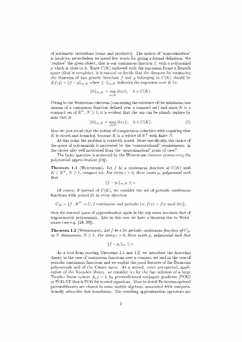
of arithmetic operations (sums and products). The notion of approximationis intuitive; nevertheless we spend few words for giving a formal denition. Wereplace the given object, that is our continuous function f , with a polynomialp which is close to it. Since C(K) endowed with the sup-norm forms a Banachspace (that is complete), it is natural to decide that the distance for measuringthe closeness of two generic functions f and g belonging to C(K) should bed(f, g) = ‖f − g‖∞,K where ‖ · ‖∞,K indicates the sup-norm over K i.e.

‖h‖∞,K = supx∈K|h(x)|, h ∈ C(K).

Owing to theWeierstrass theorem (concerning the existence of the minimum/ma-ximum of a continuous function dened over a compact set) and since K is acompact set of RN , N ≥ 1, it is evident that the sup can be plainly replace bymax that is

‖h‖∞,K = maxx∈K|h(x)|, h ∈ C(K). (1)

Here we just recall that the notion of compactness coincides with requiring thatK is closed and bounded, because K is a subset of RN with nite N .

At this point the problem is correctly posed. More specically, the choice ofthe space of polynomials is motivated by the computational requirements. Isthe choice also well motivated from the approximation point of view?

The latter question is answered by the Weierstrass theorem (concerning thepolynomial approximation [19]).

Theorem 1.1 (Weierstrass). Let f be a continuous function of C(K) withK ⊂ RN , N ≥ 1, compact set. For every ε > 0, there exists pε polynomial suchthat

‖f − pε‖∞,K ≤ ε.

Of course, if instead of C(K), we consider the set of periodic continuousfunctions with period 2π in every direction

C2π = f : RN → C, f continuous and periodic i.e. f(x) = f(x mod 2π),

then the natural space of approximation again in the sup norm becomes that oftrigonometric polynomials. Also in this case we have a theorem due to Weier-strass (see e.g. [19, 39]).

Theorem 1.2 (Weierstrass). Let f be a 2π periodic continuous function of C2π

in N dimensions, N ≥ 1. For every ε > 0, there exists pε polynomial such that

‖f − pε‖∞ ≤ ε.

As a tool from proving Theorems 1.1 and 1.2, we introduce the Korovkintheory in the case of continuous functions over a compact set and in the case ofperiodic continuous functions and we exploit the good features of the Bernsteinpolynomials and of the Cesaro sums. As a second, more unexpected, appli-cation of the Korovkin theory, we consider its for the fast solution of a largeToeplitz linear system Anx = b, by preconditioned conjugate gradients (PCG)or PCG-NE that is PCG for normal equations. More in detail Frobenius-optimalpreconditioners are chosen in some matrix algebras, associated with computa-tionally attractive fast transforms. The resulting approximation operators are

2

linear and positive and the use of a properly modied Korovkin theorem is thekey for proving the spectral clustering of the Frobenius-optimal preconditionedmatrix-sequence. As a consequence, the resulting PCG shows superlinear con-vergence behavior under mild additional assumptions.

The notes are organized as follows. In section 2 we report some basic de-nitions and tools. In Section 3 we report the Korovkin theorem, its proof, andsome basic variants, whose analysis is completed in the last two appendices (seealso the exercises in Section 10). Then, with the help of the Korovkin theory andof the Bernstein polynomials presented in Section 4.1, we produce a construc-tive proof of Theorem 1.1 in Section 4. As a byproduct, we furnish a tool forproving theorems of Weierstrass type in many dierent contexts (dierent spacesendowed with various norms, topologies, dierent models of approximation etc).As a second, more unexpected, application we show in Section 5 the use of theKorovkin theory for the fast solution of a large Toeplitz linear system Anx = b,by preconditioned conjugate gradients (PCG). More in detail Frobenius-optimalpreconditioners are chosen in some proper matrix algebras. The resulting ap-proximation operators are linear and positive and the use of a properly modiedKorovkin theorem is the key for proving the spectral clustering of the Frobenius-optimal preconditioned matrix-sequence. As a consequence, the resulting PCGshows superlinear convergence behavior under mild additional assumptions. Aconclusion section ends the notes (Section 6), together with three appendices(Sections 7, 8 , and 9) and a section devoted to exercises (Section 10).

2 Preliminary denitions and notions

We present the Korovkin theorem [17, 19]. We emphasize the simplicity of theassumptions, the possibility of their plain checking, the strength of the thesiswhich can be adapted in a variety of settings (dierent spaces endowed withvarious norms, topologies, dierent models of approximation etc).

More specically, given a sequence of operators from C(K) in itself, it issucient to verify their linearity and positivity and their convergence to g,when applied to g, for a nite number of test functions g (which can be chosenas simple polynomials). The conclusion is the pointwise convergence to theidentity over C(K), that is the convergence for any continuous function. Lastbut not the least the proof can be made very essential with tools of elementaryCalculus.

We now start with the basic denition of linear positive operator (LPO)and with denition of sequence of approximating operators (for giving a precisenotion to the pointwise convergence to the identity).

Denition 2.1. Let S be a vector space of functions with values in the eld K(with K being either R or C) and let Φ be an operator from S to S. We denethe pair of properties of Φ:

1. for any choice of α and β in K and for any choice of f e g in S, we haveΦ(αf + βg) = αΦ(f) + βΦ(g) (linearity);

2. for any choice of f ≥ 0, f ∈ S, we have Φ(f) ≥ 0 (positivity).

An operator Φ satisfying both conditions is linear and positive. We write inshort LPO.

3

Denition 2.2. Let (S, ‖ · ‖) be a Banach space of functions with values in theeld K (with K being either R or C) and let Φn be a sequence of operators eachof them from S in S. The sequence is a sequence of approximating operators or,more briey an approximation process, if for every f ∈ S we have

limn→∞

‖Φn(f)− f‖ = 0.

(In other words Φn converges pointwise to the identity operator from (S, ‖ · ‖)into itself).

3 Korovkin Theorem

In its simplest one-dimensional version the Korovkin theorem says that if asequence of LPOs (see Denition 2.1) applied to g approximates uniformly g,with g being one of the test functions 1, x, and x2, then it approximates allcontinuous functions, that is the sequence represents an approximation of theidentity operator, from the space of the continuous functions into itself, in thesense of Denition 2.2.

Theorem 3.1. Let K be a compact subset ∈ R and let Φn be a sequence oflinear and positive operators Φn : C(K)→ C(K) on the Banach space (C(K), ‖·‖∞,K). Assume that

||Φn(g)− g||∞,K → 0, for n→∞, ∀g ∈ 1, x, x2,

or Φn(g) approximates the function g as n goes to innity (this is called theKorovkin test). Then

||Φn(f)− f ||∞,K → 0, for n→∞, ∀f ∈ C(K),

or Φn(f) approximates all continuous functions dened over a compact set K,as n tends to innity.

Proof The given assumption on the test functions

||Φn(g)− g||∞,K → 0, for n→∞,

can be written asΦn(g(y))(x) = g(x) + εn(g(y))(x)

where εn(g(y))(x) represents the error we make approximating g(x) with Φn(g(y))(x)and hence it is such that ||εn(g(y))||∞,K → 0. We want to prove that

||Φn(f)− f ||∞,K → 0 for n→∞, ∀f ∈ C(K)

and therefore we x f ∈ C(K) and ε > 0, and, equivalently to the thesis, we wantto prove that there exists n (as a function of f and ε) such that for any n ≥ nand for every x ∈ K we have |Φn(f(y))(x)−f(x)| < ε. Therefore we manipulatethe latter quantity and more precisely we write ∆n(f)(x) = |Φn(f(y))(x)−f(x)|and

∆n(f)(x) = |Φn(f(y))(x)− 1 · f(x)|= |Φn(f(y))(x)− (Φn(1)(x)− εn(1)(x))f(x)| (2)

4

since 1 = Φn(1)(x)− ε(1)n (x).

Using the triangle inequality, from (2) and by using linearity rst and thenagain the triangle inequality, we obtain that

∆n(f)(x) ≤ |Φn(f(y))(x)− Φn(1)f(x)|+ |f(x)||εn(1)(x)|≤ |Φn(f(y))(x)− Φn(1)f(x)|+ ‖f‖∞,K‖εn(1)‖∞,K= |Φn(f(y))(x)− Φn(f(x))(x)|+ ‖f‖∞,K‖εn(1)‖∞,K≤ |Φn(f(y)− f(x))(x)|+ ‖f‖∞,K‖εn(1)‖∞,K .

We exploit again the positivity of Φn(·) and we nd

∆n(f)(x) ≤ Φn(|f(y)− f(x)|)(x) +ε

4, ∀n ≥ n1

since ‖ε(1)n(x)‖∞,K → 0 for n tending to ∞.The idea of the proof is to bound from above the quantity |f(y) − f(x)|,

uniformly with respect to x, y ∈ K and using only test functions.We preliminarily observe that if K is a compact set then C(K) = UC(K),

with UC(K) denoting the set of all uniformly continuous functions. As a con-sequence we have

∀ε > 0 ∃δ > 0 : |x− y| < δ ⇒ |f(x)− f(y)| < ε ∀x, y ∈ K

(the Cantor Theorem stating that continuity and uniform continuity are thesame notion, when the domain is compact).Thus, in general, we obtain |f(x) − f(y)| ≤ ε if the points x and y are closeenough. The latter condition can be rewritten as follows

|f(x)− f(y)| ≤ εχz:|z−x|<δ(y) + 2||f ||∞,Kχz:|z−x|≥δ(y).

However the righthand-side is not continuous, and it cannot be in general anargument for the operator Φn(·). We want to majorize it by using a contin-uous function: we will succeed by nd a bound from above made by linearcombinations of the test functions. First we observe that

|z − x| ≥ δ ⇔ |z − x|δ

≥ 1,

which in turn is equivalent to

(z − x)2

δ2≥ 1

In conclusion in the set the inequality is satised we can write

χz:|z−x|≥δ(y) = 1 ≤ (y − x)2

δ2.

Otherwise we have

χz:|z−x|≥δ(y) = 0 ≤ (y − x)2

δ2.

5

Therefore, uniformly with respect to x, y ∈ K, for any ε > 0 we nd δ = δε 0such that

|f(x)− f(y)| ≤ ε+ 2‖f‖∞,K(y − x)2

δ2.

Hence, by applying the operator Φn(·), for every n ≥ n1 we nd that

∆n(f)(x) ≤ ε

4+ Φn

(ε+ 2

‖f‖∞,Kδ2

(y − x)2

)(x)

=ε

4+ εΦn(1)(x) + 2

‖f‖∞,Kδ2

Φn(y2 − 2xy + x2)(x). (3)

Moreover Φn(1)(x) = (1 + εn(1)(x)) since the constant 1 is a test function.Therefore the righthand-side in (3) can be written as

ε

4+ε(1+εn(1)(x))+2

‖f‖∞,Kδ2

x2+εn(y2)(x)−2x[x+εn(y)(x)]+x2(1+εn(1)(x)).

Now we choose ε = ε4 and we observe that, by denition of limit, there exist

n2, n3 such that for n ≥ n2 we have εn(1)(x) ≤ 1, uniformly with respect tox ∈ K, and for n ≥ n3 we have

‖f‖∞,K‖εn(y2)(x)− 2xεn(y)(x) + x2εn(1)(x)‖∞,K ≤δ2ε

2.

Finally the proof is concluded by taking n ≥ n, with n = maxn1, n2, n3(depending on both f and ε), and by observing that

∆n(f)(x) ≤ ε

4+2ε+2

‖f‖∞,Kδ2

εn(y2)(x)−2xεn(y)(x)+x2εn(1)(x) ≤ ε

4+3ε = ε.

2

In the following section, in order to prove the Weierstrass Theorem, we willpropose some special polynomial sequence of linear positive operators Φnsatisfying the Korovkin test (with Φn(f) being a polynomial for every f ∈C(K)). However we should not forget that the Korovkin Theorem is very general(and exible). Indeed no assumptions are required on the regularity of Φn(f).In reality, by following step by step the proof given above, we discover thatproof is still valid even if Φn(f) is not necessarily continuous. In fact we onlyneed that it makes sense to write ‖Φn(f)‖∞,K or equivalently that Φn(f) isessentially bounded (Φn(f) ∈ L∞(K)).

3.1 Few variations and a list of applications

As anticipated in the last section, the Korovkin Theorem is very exible. Herewe list a few changes that can be made by obtaining a rich series of new state-ments. Then we list a series a interesting applications

First Case: LetK be a compact subset of RN and T = 1, x1, x2, . . . , xN , ‖x‖22the set of test functions. The proof of theorem is formally the same, but xmust be regarded as a vector of size N . Regarding the uniform continuitythe right characterization to be chosen is as follows

∀ε > 0 ∃δ > 0 : ‖x− y‖2 < δ ⇒ |f(x)− f(y)| < ε ∀x, y ∈ K.

6

As a consequence the key majorization is the one reported below.

|f(y)− f(x)| ≤ εχz:||z−x||2≤δ(y) + 2‖f‖∞,K χz:||z−x||2≥δ(y)

≤ ε+ 2‖f‖∞,K‖y − x‖22

δ2, (4)

since ‖z − x‖2 ≥ δ ⇒ ‖z−x‖22δ2

≥ 1. Noting that

‖y − x‖22 = (yT − xT )(y − x) = ‖x‖22 + ||y||22 − 2

d∑j=1

xjyj

we conclude that the function appearing in (4), with respect to the dummyvariable y, is just a linear combination of test functions and therefore therest of the proof is identical (see Appendix B).

Second Case: Let C2π be the set of 2π-periodic functions. The set of thetest functions is given by

T = 1, e√−1x.

We also use the function e−√−1x but since it is the conjugate of the second

test function we do not need to put it in the Korovkin test. Indeed, if fis real valued then f = f+ − f− with f+ = max0, f, f− = max0,−fbeing both nonnegative so that Φ(f) is real valued if f is and Φ(·) is linearand positive. As a consequence, for a general complex valued function f wehave Φ(f) = ¯Φ(f). Taking into account the latter, the proof only changeswhen reasoning about the uniform continuity. A possible distance betweenx and y is dened as

|e√−1x − e

√−1y|.

As a consequence a clever characterization of the notion of uniform conti-nuity is given as

∀ε > 0 ∃δ > 0 : |e√−1x − e

√−1y| ≤ δ ⇒ |f(x)− f(y)| < ε ∀x, y ∈ R.

Hence the key upper-bound is

|f(y)− f(x)| ≤ εχy:|e√−1x−e

√−1y|≤δ(y) + 2‖f‖∞ χy:|e

√−1x−e

√−1y|≥δ(y)

≤ ε+ 2‖f‖∞|e√−1x − e

√−1y|2

δ2

≤ ε+ 2‖f‖∞δ2

(2− e−√−1xe

√−1y − e

√−1xe−

√−1y),

since|e√−1x − e

√−1y|2

δ2≥ 1,

where 2− e−√−1xe

√−1y − e

√−1xe−

√−1y is the linear combination of test

functions, with regard to the dummy variable y (see Appendix C, also forthe multivariate setting).

7

Third case: With reference to Theorem 3.1, the Korovkin set T = 1, x, x2can be replaced by any Chebyshev set C = p0(x), p1(x), p2(x) of continu-ous functions over the compact setK such that the 3×3 Vandermonde-likematrix

(pj(xk))j,k=0,1,2

is invertible for every choice of points xk such that x0 < x1 < x2,x0, x1, x2 ∈ K. It is worth noticing that an analogous result does not holdin more than one dimension, due to topological reasons (see Exercise 12).

As already stressed in the introduction, among classical applications of theKorovkin theory, we can list the rst and the second Weierstrass Theorems(a huge variety of applications in approximation theory can be found in thework by Altomare and coauthors [1]). As a more exotic application we nallymention the use of the Korovkin tools in the approximation of Toeplitz matrixsequences via (computationally simpler) matrix algebras [25], including the setof circulant matrices associated to the celebrated fast Fourier transform (FFT).The corresponding Korovkin test is successfully veried for all ω-circulants with|ω| = 1, with all known sine, cosine, and Hartley transform spaces (see [10, 11,2]) and is extended to the case of block structures [26] and to some operatortheory settings [18]: to the matrix version setting we devoted the analysis inSection 5.

4 Proof of the Weierstrass Theorem

In this section we rst introduce the Bernsterin polynomials (and the relatedsequence of operators) and we prove linearity, positivity and the proof of thepositive answer to the Korovkin test. The we give a (semi)-constructive proofof the Weierstrass Theorem. The only non-constructive tool concerns the useof the Tietze extension Theorem (see [21]).

4.1 The Bernstein polynomials

We furnish a concrete example of a sequence of linear positive operators. Wewill perform the Korovkin test. For the sake of simplicity we rst consider theone-dimensional case with N = 1 and K = [0, 1]. The Bernstein polynomials off , indicated by Bn(f), are dened as

Φn(f)(x) ≡ Bn(f)(x) =

n∑ν=0

(nν

)xν(1− x)n−νf

(νn

). (5)

It is straightforward to verify that it is a linear and positive operator, sinceit is expressed as linear combination of nonnegative polynomials xν(1 − x)n−ν

of degree n, via the coecients (nν

)f(νn

),

which are all nonnegative if f ≥ 0. From these remarks we immediately getboth positivity and linearity of the operator Bn.

8

4.1.1 Bernstein polynomials and Korovkin test

We now perform the Korovkin test. For g ∈ 1, x, x2 we prove that Bn(g)converges uniformly to g on [0, 1].

For g = 1 we have

Bn(1)(x) =

n∑ν=0

(nν

)xν(1− x)n−ν

= (x+ (1− x))n = 1

and thus the error εn(1) is identically zero.For g(x) = x we have

Bn(g(y))(x) =

n∑ν=0

(nν

)xν(1− x)n−ν

ν

n

=

n∑ν=1

n!

ν!(n− ν)!

ν

nxν(1− x)n−ν

=

n∑ν=1

(n− 1ν − 1

)xν(1− x)n−ν

=

n−1∑q≡ν−1=0

(n− 1q

)xq+1(1− x)n−1−q

= xBn−1(1)(x) = x

and hence, also in this case, the error εn(y) is identically zero.Finally we consider g(x) = x2 so that

Bn(g(y))(x) =

n∑ν=0

(nν

)xν(1− x)n−ν

ν2

n2

=

n∑ν=0

(nν

)xν(1− x)n−ν

ν(ν − 1)

n2

+

n∑ν=0

(nν

)xν(1− x)n−ν

ν

n2

=

n∑ν=2

(nν

)xν(1− x)n−ν

ν(ν − 1)

n2+

1

nBn(y)(x)

=n− 1

n

n∑ν=2

(nν

)xν(1− x)n−ν

ν(ν − 1)

n(n− 1)+

1

nx

=n− 1

n

n∑ν=2

(n− 2ν − 2

)xν(1− x)n−ν +

1

nx

=n− 1

n

n−2∑q≡ν−2=0

(n− 2q

)xq+2(1− x)n−2−q +

1

nx

=n− 1

nx2Bn−2(1)(x) +

1

nx =

n− 1

nx2 +

1

nx

= x2 +x(1− x)

n.

9

In conclusion the error εn(y2)(x) = x(1−x)n converges uniformly to zero so that

the test of Korovkin has a positive answer. Then, by invoking the KorovkinTheorem, we deduce that Bn is an approximation process on C([0, 1], ‖ · ‖∞).

Remark 4.1. We note that the error is identically zero for the rst and secondtest functions. If the error in the third test function would have been identicallyzero, then we would have concluded

Bn(f(y))(x) = f(x), ∀f, x, n.

Hence C(K) would coincide with space of polynomials: the latter is clearly nottrue, so we necessarily expected a non-zero error for j = 2 (refer to Exercise 2and also Exercise 3 for a deeper understanding on the results).

4.1.2 The case of the multidimensional Bernstein polynomials

We generalize the notion of Bernstein polynomial in the multidimensional set-ting. We considerK = [0, 1]N and on this set we dene the Bernstein polynomialof f denoted by Bn(f), with n = (n1, . . . , nN ) multi-index:

Bn(f(y))(x) =

n1∑ν1=0

· · ·nN∑νN=0

(n1

ν1

)· · ·(nNνN

)(6)

xν1(1− x)n1−ν1 · · ·xνN (1− x)nN−νN f

(ν1

n1, . . . ,

νNnN

).

It is trivial to verify that the given operator is linear and positive since it isa linear combination of nonnegative polynomials of degree n

xν1(1− x)n1−ν1 · · ·xνN (1− x)nN−νN

via the coecients (n1

ν1

)· · ·(nNνN

)f

(ν1

n1, . . . ,

νNnN

),

which are all nonnegative if f ≥ 0. From these observations both linearity andpositivity directly follow.

4.2 A Korovkin based proof of the Weierstrass Theorem

We prove Theorem 1.1 of which we recall once again the statement and then weproceed with its proof based on the Korovkin theory.

Let f be any function belonging to C(K) with K ⊂ RN , N ≥ 1, compactset. For every ε > 0 there exists pε polynomial such that

‖f − pε‖∞,K ≤ ε.

Proof The proof is organized by steps and more precisely by treating the caseof a domain K of increasing complexity.Step 1: K = [0, 1]

10

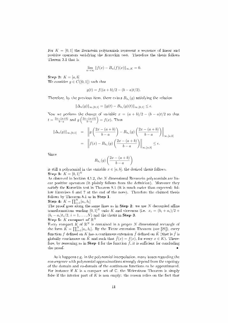
For K = [0, 1] the Bernstein polynomials represent a sequence of linear andpositive operators satisfying the Korovkin test. Therefore the thesis followsTherem 3.1 that is

limn→∞

‖f(x)−Bn(f)(x)‖∞,K = 0.

Step 2: K = [a, b]We consider g ∈ C([0, 1]) such that

g(t) = f((a+ b)/2− (b− a)t/2).

Therefore, by the previous item, there exists Bnε(g) satisfying the relation

‖∆n(g)‖∞,[0,1] = ‖g(t)−Bnε(g)(t)‖∞,[0,1] ≤ ε.

Now we perform the change of variable x = (a + b)/2 − (b − a)t/2 so that

t = 2x−(a+b)b−a and g

(2x−(a+b)b−a

)= f(x). Thus

‖∆n(g)‖∞,[0,1] =

∥∥∥∥g(2x− (a+ b)

b− a

)−Bnε(g)

(2x− (a+ b)

b− a

)∥∥∥∥∞,[a,b]

=

∥∥∥∥f(x)−Bnε(g)

(2x− (a+ b)

b− a

)∥∥∥∥∞,[a,b]

≤ ε.

Since

Bnε(g)

(2x− (a+ b)

b− a

)is still a polynomial in the variable x ∈ [a, b], the desired thesis follows.Step 3: K = [0, 1]N

As observed in Section 4.1.2, the N dimensional Bernstein polynomials are lin-ear positive operators (it plainly follows from the denition). Moreover theysatisfy the Korovkin test in Theorem 8.1 (it is much easier than expected: fol-low Exercises 6 and 7 at the end of the note). Therefore the claimed thesisfollows by Theorem 8.1 as in Step 1.Step 4: K =

∏Ni=1[ai, bi]

The proof goes along the same lines as in Step 2: we use N decoupled anetransformations sending [0, 1]N onto K and viceversa (i.e. xi = (bi + ai)/2 +(bi − ai)ti/2, i = 1, . . . , N) and the thesis in Step 3.Step 5: K compact of RNEvery compact K of RN is contained in a proper N dimensional rectangle ofthe form K =

∏Ni=1[ai, bi]. By the Tietze extension Theorem (see [21]), every

function f dened on K has a continuous extension f dened on K (that is f isglobally continuous on K and such that f(x) = f(x), for every x ∈ K). There-fore, by reasoning as in Step 4 for the function f , it is sucient for concludingthe proof. •

As it happens e.g. in the polynomial interpolation, many issues regarding theconvergence with polynomial approximations strongly depend from the topologyof the domain and co-domain of the continuous functions to be approximated.For instance if K is a compact set of C, the Weierstrass Theorem is simplyfalse if the interior part of K is non emply: the reason relies on the fact that

11

the uniform limit over any compact contained in a given open domain Ω of asequence of holomorphic functions over Ω (e.g. a sequence of polynomials withΩ being the internal part of K) is still holomorphic over Ω.

4.3 An historical note: the original proof given by Weier-

strass

In this section we sketch the original proof provided by Weierstrass in his work.Of course the proof is not explicitly based on the theory of linear positive oper-ators (the Korovkin theory is more recent and is dated around 1958-1960), butit uses a special sequence of linear positive operators that is those of Gauss-Weierstrass.

The n-th Gauss-Weiertrass operator is dened as

(GWn(f))(x) =

√n

2π

∫ ∞−∞

e−n(t−x)2

2 f(t)dt. (7)

Unlike the Bernstein case, we observe that (GWn(f))(x) is not a polynomialin general but it is a smooth function belonging to C∞ on the whole real lineR (thanks to the role of a Gaussian weight).

The remaining part of the proof follows according to the ideas describedbelow:Step 1. We take the Taylor polynomial pn,m(x) of degree m associated with(GWn(f))(x) and it is possible to prove that

limm→∞

‖(GWn(f))(x)− pn,m(x)‖∞,K = 0

for every compact K of R.Step 2. It is possible to prove that (GWn(f))(x) converges uniformly to f(x)for every compact K of R, as n tends to innity.

The two considered steps imply the Weierstass Theorem for every compactK of R. It should be mentioned that the proof is only partially constructivesince pn,m is dened using information on f not available in general (except vianumerical evaluations).

5 Application of the Korovkin theory to precon-ditioning

This section deals with some applications of Korovkin theory to the precondi-tioning, since we are interested to design fast iterative solvers when the size nof our linear system is large. More in detail we consider the case of Toeplitzmatrices and we show that the approximation of such matrices in specic ma-trix algebras can be reduced, at least asymptotically, to a single test on theshift matrix: the idea behind this surprising simplication is the use of the Ko-rovkin machinery on the spectrum of the matrices approximating the Toeplitzstructures.

The section is organized into three parts: in the rst we give preliminarydenitions and tools, in the second we present Toeplitz matrices, the space ofapproximation, and the approximation strategy and nally in the third part westate and prove the Korokvin theorem in the setting of Toeplitz matrix sequenceswith continuous symbol.

12

5.1 Denitions and tools

Denition 5.1. A matrix sequence An, An square matrix of size n, is clus-tered at s ∈ C (in the eigenvalue sense), if for any ε > 0 the number of theeigenvalues of An o the disk

D(s, ε) := z : |z − s| < ε

is o(n). In other words

qε(n, s) := #λj(An) : λj /∈ D(s, ε) = o(n), n→∞.

If every An has only real eigenvalues (at least for all n large enough), then s isreal and the disk D(s, ε) reduces to the interval (s−ε, s+ε). The cluster is strongif the term o(n) is replace by O(1) so that the number of outlying eigenvalues isbounded by a constant not depending on the size n of the matrix.

We say that a preconditioner Pn is optimal for An if the sequence P−1n An

is clustered at one (or to any positive constant) in the strong sense. Since

P−1n An = In + P−1

n (An − Pn),

it is evident that for the optimality we need to prove the strong cluster at zero ofAn−Pn; for details on this issue refer to [12]; in addition several useful resultson preconditioning can be found in [3, 20], while in [15, 23] the reader can nda rich account on general Krylov methods. The (weak or general) clustering isalso of interest, as a heuristic indication that the preconditioner is eective.

Remark 5.2. The previous Denition 5.1 can be stated also for the singularvalues instead of the eigenvalues just replacing λ with σ and eigenvalue withsingular value.

Given a matrix A we dene the Schatten p norm, p ∈ [1,∞), as the p norm

of the vector of its singular values i.e. ‖A‖S,p =[∑n

j=1 σpj (A)

]1/p. By taking a

limit on p the Schatten ∞ norm is exactly the spectral norm i.e. the maximalsingular value. Among these norms the one which interesting both from acomputational viewpoint and from a theoretical viewpoint is the Schatten 2norm which is called the Frobenius norm in the Numerical Analysis community.We dene now the Frobenius norm as it is usually dened in a computationalsetting

‖A‖F =

n∑j,k=1

|Aj,k|21/2

. (8)

Of course if A is replaced by QA with Q unitary matrix, then every columnwill maintain the same Euclidean length and therefore ‖QA‖F = ‖A‖F ; on theother hand, if A is replaced by AP with P unitary matrix, then every rowwill maintain the same Euclidean length and therefore ‖AP‖F = ‖A‖F . Thesetwo statements show that ‖ · ‖F is a unitarily invariant (u.i.) norm so that‖QAP‖F = ‖A‖F for every matrix A and for every unitary matrices P andQ; a rich and elegant account on the properties of such norms can be found in[5]. Therefore, taking into account the singular value decomposition [14] of A

13

and choosing P and Q as the transpose conjugate of the left and right vectorsmatrices, we conclude that ‖A‖F = ‖Σ‖F with Σ being the diagonal matrix withthe singular values σ1(A) ≥ σ2(A) ≥ · · · ≥ σn(A) on the diagonal. Therefore

‖ · ‖F = ‖ · ‖S,2,

so that the Schatten 2 norm has a very nice computational expression that onlydepends on the entries of the matrix. Furthermore the denition in (8) revealsthat ‖A‖2F = 〈A,A〉, with 〈A,B〉 = trace(B∗A) being the (positive) Frobeniusscalar product. Therefore the Frobenius norm comes from a positive scalarproduct and consequently the space of the matrices of size n with the Schatten2 norm is a Hilbert space: this further property represents a second importantingredient for the strategy of approximation that we follow in order to obtain agood preconditioner.

The following lemma links the notion of clustering with a quantitative esti-mate of the Schatten p norms.

Lemma 5.3. Assume that a sequence of matrices Xn is given and that‖Xn‖S,p = O(1) for some p ∈ [1,∞). Then Xn is clustered at zero in thestrong sense.

Proof The assumption implies that there exist a constant M such that‖Xn‖S,p ≤M for n large enough. Consequently the proof reduces to a series ofinequalities as shown below

Mp ≥ ‖Xn‖S,p (by the assumption ‖Xn‖S,p ≤M, n ≥ n)

=

n∑j=1

σpj (Xn) (by definition of ‖ · ‖S,p)

≥∑

j:σj(Xn)>ε

σpj (Xn) (for any fixed ε > 0)

≥∑

j:σj(Xn)>ε

εp

= εp#j : σj(Xn) > ε.

Therefore, for every ε > 0, we have proved that the cardinality of the set ofsingular values of Xn exceeding ε, for n large enough, is bounded by the con-stant (M/ε)p which, by denition, is equivalent to write that Xn is clusteredat zero in the strong sense. •

The result above is nicely complemented by the following remark.

Remark 5.4. With reference to Lemma 5.3, if the assumption that ‖Xn‖S,p =O(1) for some p ∈ [1,∞) is replaced by the weaker request that ‖Xn‖S,p = o(n)for some p ∈ [1,∞), then the same proof of the lemma shows that Xn isclustered at zero in the weak sense.

14

5.2 Toeplitz sequences, approximating spaces, and approx-

imation strategy

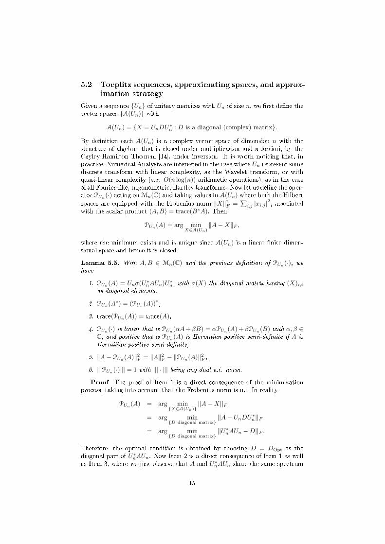
Given a sequence Un of unitary matrices with Un of size n, we rst dene thevector spaces A(Un) with

A(Un) = X = UnDU∗n : D is a diagonal (complex) matrix.

By denition each A(Un) is a complex vector space of dimension n with thestructure of algebra, that is closed under multiplication and a fortiori, by theCayley-Hamilton Theorem [14], under inversion. It is worth noticing that, inpractice, Numerical Analysts are interested in the case where Un represent somediscrete transform with linear complexity, as the Wavelet transform, or withquasi-linear complexity (e.g. O(n log(n)) arithmetic operations), as in the caseof all Fourier-like, trigonometric, Hartley transforms. Now let us dene the oper-ator PUn(·) acting on Mn(C) and taking values in A(Un) where both the Hilbert

spaces are equipped with the Frobenius norm ‖X‖2F =∑i,j |xi,j |

2, associated

with the scalar product 〈A,B〉 = trace(B∗A). Then

PUn(A) = arg minX∈A(Un)

‖A−X‖F ,

where the minimum exists and is unique since A(Un) is a linear nite dimen-sional space and hence it is closed.

Lemma 5.5. With A,B ∈ Mn(C) and the previous denition of PUn(·), wehave

1. PUn(A) = Unσ(U∗nAUn)U∗n, with σ(X) the diagonal matrix having (X)i,ias diagonal elements,

2. PUn(A∗) = (PUn(A))∗,

3. trace(PUn(A)) = trace(A),

4. PUn(·) is linear that is PUn(αA+ βB) = αPUn(A) + βPUn(B) with α, β ∈C, and positive that is PUn(A) is Hermitian positive semi-denite if A isHermitian positive semi-denite,

5. ‖A− PUn(A)‖2F = ‖A‖2F − ‖PUn(A)‖2F ,

6. ‖|PUn(·)‖| = 1 with ‖| · ‖| being any dual u.i. norm.

Proof The proof of Item 1 is a direct consequence of the minimizationprocess, taking into account that the Frobenius norm is u.i. In reality

PUn(A) = arg minX∈A(Un)

||A−X||F

= arg minD diagonal matrix

||A− UnDU∗n||F

= arg minD diagonal matrix

||U∗nAUn −D||F .

Therefore, the optimal condition is obtained by choosing D = DOpt as thediagonal part of U∗nAUn. Now Item 2 is a direct consequence of Item 1 as wellas Item 3, where we just observe that A and U∗nAUn share the same spectrum

15

by similarity (U∗n is the inverse of Un). The rst part of item 4 is again a directconsequence of the representation formula in Item 1, while for the second partwe just observe that the positive semi-deniteness of A is equivalent to thatof U∗nAUn so that its diagonal σ(U∗nAUn) is made up by nonnegative numberswhich are the eigenvalues of the Hermitian matrix PUn(A). Item 5 is nothing butthe Pythagora law holding in any Hilbert space. The proof of Item 6 is reducedto prove ‖|PUn(A)‖| ≤ ‖|A‖| for every complex matrix, since PUn(I) = I. Thegeneral result is given in [28], thanks to a general variational principle. For thesubsequent purposes we need in fact only the statement for the spectral norm.In that case, using the singular value decomposition [14], it is easy to see that

‖A‖ = max‖u‖2=‖v‖2=1

|v∗Au|, (9)

so that

‖A‖ = max‖u‖2=‖v‖2=1

|v∗Au|

≥ maxi=1,...,n

|u∗iAui|

= ‖PUn(A)‖with u1, . . . , un being the orthonormal columns forming Un and where in the lastequality we used the key representation formula in Item 1. We nally observethat ‖PUn‖F = 1 is a direct consequence of the Pythagora law in Item 5. •

We will apply the former projection technique to Toeplitz matrix-sequencesTn where the n-th matrix Tn is of the form

(Tn)j,k = aj−k(f) (10)

with aj , j ∈ Z, given coecients. In the following we are interested to the casewhere, given f ∈ L1(0, 2π), the entries of the matrix Tn are dened via theFourier coecients of f that is

aj =1

2π

∫ 2π

0

f(t)e−√−1jt dt.

The latter denes a sequence Tn(·) of operators, Tn : L1(0, 2π) → Mn(C),which are clearly linear, due to the linearity of the Fourier coecients, andpositive as proved in detail below. In fact, if f is real valued then it is immediateto see that the conjugate of aj is exactly a−j so that by (10) we deduce thatT ∗n(f) = Tn(f). Now we observe that for any pair of vector u and v (with entriesindexed from 0 to n− 1) we have the identity

v∗Tn(f)u =

n−1∑j,k=0

vj(Tn(f))j,kuk

=

n−1∑j,k=0

vjaj−k(f)uk

=1

2π

∫ 2π

0

f(t)

n−1∑j,k=0

vjuke−√−1jte

√−1kt dt

=1

2π

∫ 2π

0

f(t)pv(t)pu(t) dt, (11)

16

where, for a given vector x of size with entries indexed from 0 to n − 1, thesymbol px(t) stands for the polynomial

px(t) =

n−1∑k=0

xke√−1kt.

It is worth noticing the the map from Cn with Euclidean norm to the spacePn−1 of polynomials of degree at most n − 1 on the unit circle with the HaarL2(0, 2π) norm is an isometry, since

‖x‖22 =1

2π

∫ 2π

0

|px(t)|2 dt. (12)

Now the positivity of the operator is a plain consequence of the integral repre-sentation in (11), since for every u ∈ Cn and every nonnegative f ∈ L1(0, 2π),we have

u∗Tn(f)u =1

2π

∫ 2π

0

f(t)|pu(t)|2 dt ≥ 0.

In fact, a little more eort (see [24]) leads to conclude u∗Tn(f)u = 0 if and onlythe nonnegative symbol f is zero a.e.

Therefore the composition of PUn(·) and Tn(·) is also a linear and positiveoperator from L1(0, 2π) to A(Un) ⊂Mn(C).

Now starting from the eigenvalues of PUn(Tn(f)) we may construct a linearpositive operator from L1(0, 2π) to C2π; in fact we will be interested mainly tothe case where f ∈ C2π so that we will consider the restriction of PUn(Tn(·)) toC2π.

The costruction proceeds as follows. Let f be a function belonging to C2π.We consider the j-th eigenvalue of PUn(Tn(f)) which is

λj(f, n) = (U∗nTn(f)Un)jj , j = 0, . . . , n− 1, (13)

which can be seen a linear positive functional with respect to the argument fthat is λj(·, n) : C2π → C is a linear positive functional. We now dene a globaloperator Φn(·) from C2π into itself as reported below

Φn(f(y))(x) =

λj(f(y), n), if x mod 2π = 2πj

nlinear interpolation at the endpoints, if x mod 2π ∈ Ij,n

for j = 0, 1, ..., n − 1, Ij,n =[

2πjn , 2π(j+1)

n

), and with λn(f, n) set equal to

λ0(f, n) = (U∗nTn(f)Un)00 for imposing periodicity. We observe that for everyf ∈ C2π the function Φn(f(t))(x) is also continuous and 2π periodic. Indeed,the operator

Φn : C2π → C2π

is linear, since the sampling points in (13) are linear functionals and the inter-polation retains the property of linearity. Furthermore if f is nonnegative, thenλj(f, n) are all nonnegative (due the positivity of all the functionals λj(·, n))and the linear interpolation preserves the non-negativity. As a conclusion, Φnis a sequence of linear positive operators from C2π into C2π and hence we canapply the Korovkin theorem in its periodic version.

17

5.3 The Korovkin theorem in a Toeplitz setting

As a nal tool we need a quantitative version of the Korovkin theorem fortrigonometric polynomials. We report it in the next lemma. Then we specializesuch a result for dealing with the operators Φn constructed from the eigenvaluefunctionals in (13) and, nally, we prove the Korovkin theorem in the Toeplitzsetting.

Lemma 5.6. Let us consider the standard Banach space C2π endowed the sup-norm. Let us denote by T = 1, e

√−1x the standard Korovkin set of 2π periodic

test functions and let us take a sequence Φn of linear positive operators fromC2π in itself. If for any g ∈ T

maxg∈T‖Φn(g)− g‖∞ = O(θn),

with θn tending to zero as n tends to innity, then, for any trigonometric poly-nomial p of xed degree (independent of n), we nd

‖Φn(p)− p‖∞ = O(θn).

Proof We rst observe that, by the linearity and by the positivity of Φn(see the discussion at the beginning of the rst item in Section 3.1), we get

‖Φn(e±√−1y)(x)− e±

√−1x‖∞ = O(θn).

Moreover, from the linearity of the space of the trigonometric polynomials,the claimed thesis is proved if we prove the statement for the monomials e±k

√−1x

for any positive xed integer k. Therefore setting w = e√−1y and z = e

√−1x we

haveΦn(wk)(x)− zk = Φn(wk)(x)− Φn(1)(x)zk +O(θn)

= Φn(wk)(x)− Φn(zk)(x) +O(θn)= Φn(wk − zk)(x) +O(θn).

Now it is useful to manipulate the dierence wk − zk. Actually the followingsimple relations hold:

wk − zk = (w − z)kzk−1 + (w − z)·(wk−1 − zk−1 + z(wk−2 − zk−2) + . . .+ zk−2(w − z))

= (w − z)kzk−1 + |w − z|2 1(w−z) ·

(wk−1 − zk−1 + z(wk−2 − zk−2) + . . .+ zk−2(w − z)).

Furthermore, setting

R(w, z) =1

(w − z)(wk−1 − zk−1 + z(wk−2 − zk−2) + . . .+ zk−2(w − z)),

we nd that

‖R(w, z)‖∞ = ‖ 1(w−z) · (w

k−1 − zk−1+

+z(wk−2 − zk−2) + . . .+ zk−2(w − z))‖∞= ‖ 1

(w−z) · (wk−1 − zk−1+

+z(wk−2 − zk−2) + . . .+ zk−2(w − z))‖∞≤

∑k−1j=1 j = (k − 1)k/2.

18

Now we exploit the linearity and the positivity of the operators Φn(·) andthe fact that z and x are constants with regard to the operator Φn(·).

|Φn(wk − zk)(x)| = |Φn((w − z)kzk−1)(x) + Φn(|w − z|2R(w, z))(x)|= |Φn(w − z)(x)kzk−1 + Φn(|w − z|2R(w, z))(x)|= |O(θn)kzk−1 + Φn(|w − z|2R(w, z))(x)|.

By linearity we have Φn(|w − z|2R(w, z))(x) = Φn(|w − z|2Re(R(w, z)))(x) +√−1Φn(|w−z|2Im(R(w, z)))(x) where Re(s) and Im(s) denote the real and the

imaginary part of s respectively. By the triangle inequality and by the positivityof Φn we deduce

|Φn(|w − z|2R(w, z))(x)| ≤ |Φn(|w − z|2Re(R(w, z)))(x)|++|Φn(|w − z|2Im(R(w, z)))(x)|

≤ Φn(|w − z|2|Re(R(w, z))|)(x)++Φn(|w − z|2|Im(R(w, z))|)(x)

≤ 2Φn(|w − z|2‖R(w, z)‖∞)(x).

Therefore, by taking into account the preceding relationships we obtain

|Φn(wk − zk)(x)| ≤ |O(θn)k|+ Φn(|w − z|2)2‖R(w, z)‖∞≤ O(θn) + Φn(|w − z|2)2‖R(w, z)‖∞≤ O(θn) + Φn(|w − z|2)(k − 1)k≤ O(θn) + Φn(2− wz − zw)(k − 1)k≤ O(θn) + (2 +O(θn))− (z +O(θn))z−−z(z +O(θn)))(k − 1)k = O(θn).

The latter, together with the initial equations, implies that

‖Φn(wk)(x)− zk‖∞ = O(θn)

and the lemma is proved. •

Here we report a specic version of the above lemma, adapted to the specicsequence Φn constructed in the previous subsection, which is more suited forthe subsequent clustering analysis.

Lemma 5.7. Let us consider the standard Banach space C2π endowed the sup-

norm, let us dene x(n)j = 2πj

n , j = 0, . . . , n − 1, and let us take the sequenceΦn of linear positive operators from C2π in itself, dened via the linear eigen-value functionals in (13). If

maxi=0,...,n−1

‖λj(e√−1x, n)− e

√−1x

(n)j ‖∞ = O(θn),

with θn = O(n−1), for n going to innity, then, for any trigonometric polyno-mial p of xed degree (independent of n), we nd

‖Φn(p)− p‖∞ = O(n−1).

Proof First of all we observe that the special nature of the operators Φnimplies that only the single test function g(x) = e

√−1x must be considered.

19

Indeed the identity matrix I belongs to the algebra A(Un) since Un is unitary.Therefore we have no error: in fact we have

g = 1⇒ Tn(1) = I ⇒ PUn(Tn(1)) = P(I) = I,

so that λj(1, n) = 1 and therefore

Φn(1)(x) ≡ 1.

As in the previous lemma, since PUn(A∗) = P∗Un(A), we have Tn(e−√−1t) =

T ∗n(e√−1t), PUn(Tn(e−

√−1t)) = P∗Un(Tn(e

√−1t)), so that

λj(e−√−1t, n) = λj(e

√−1t, n)

that is in generalΦn(f) = Φn(f).

The proof now is reduced to the application of Lemma 5.6, if we prove thatthe given assumption

maxi=0,...,n−1

‖λj(e√−1x, n)− e

√−1x

(n)j ‖∞ = O(θn)

implies

‖Φn(e√−1y)(x)− e

√−1x‖∞ = O(n−1)

uniformly with respect to x ∈ R. The proof is plain. In fact let h(x) = e√−1x.

Then q(x) = Φn(e√−1y)(x) is continuous, 2π periodic, piecewise linear, and

such that |h(x) − q(x)| = O(θn) uniformly for x = x(n)j . We have to prove the

same estimate for x ∈ (x(n)j , x

(n)j+1). We have

h(x)− q(x) = h(x)− h(xj) + h(x(n)j )− q(x(n)

j ) + q(x(n)j )− q(x)

= α1 + α2 + α3,

where

α1 = h(x)− h(x(n)j ),

α2 = h(x(n)j )− q(x(n)

j ),

α3 = q(x(n)j )− q(x).

Now |α2| = O(θn) by hypothesis, |α3| = O(n−1) because q is a piecewise lin-ear function, almost interpolating with error O(θn) the Lipschitz continuousfunction h, where the latter observation or a direct Taylor expansion implies|α3| = O(n−1). •

Theorem 5.8. Let us consider the standard Banach space C2π endowed the

sup-norm, let us dene x(n)j = 2πj

n , j = 0, . . . , n − 1, and let us take the se-quence Φn of linear positive operators from C2π in itself, dened via the lineareigenvalue functionals in (13). If

maxi=0,...,n−1

‖λj(e√−1x, n)− e

√−1x

(n)j ‖∞ = O(θn),

with θn tending to zero, as n tends to innity, then for every f ∈ C2π thesequence Tn(f)− PUn(Tn(f)) is weakly clustered at zero.

20

Proof By denition of clustering (see Denition 5.1) and taking into con-sideration the singular value decomposition, see [14], given f ∈ C2π, the thesisamounts in proving that, for every ε > 0, there exist sequences Nn,ε andRn,ε such that

Tn(f)− PUn(Tn(f)) = Nn,ε +Rn,ε, (14)

with ‖Nn,ε‖ < ε and rank(Rn,ε) ≤ r(ε)n with

limε→0

r(ε) = 0.

We take a generic function f ∈ C2π. By virtue of the secondWeierstrass theorem(i.e. Theorem 1.2 with N = 1), for every δ > 0 there exists pδ for which

‖f − pδ‖∞ < δ

where pδ is a trigonometric polynomial. Hence, taking into account the linearityof PUn(·) and Tn(·) proved in Section 5.2, we obtain

Tn(f)− PUn(Tn(f)) = Tn(f)− Tn(pδ) + Tn(pδ)− PUn(Tn(pδ))

+PUn(Tn(pδ))− PUn(Tn(f))

= Tn(f − pδ) + Tn(pδ)− PUn(Tn(pδ)) + PUn(Tn(Pδ − f))

= E1 + E2 + E3,

where E1 = Tn(f − pδ), E2 = Tn(pδ)−PUn(Tn(pδ)), E3 = PUn(Tn(Pδ − f)) arethe error terms. At this point we observe that relations (9) and (11) implies

‖E1‖ ≤ ‖f − pδ‖∞ < δ

, while the previous inequality and Item 6 in Lemma 5.5, with the choice of thespectral norm, leads to

‖E3‖ ≤ ‖E1‖ < δ.

Now we must prove handle the term E2 and for it we consider the Frobeniusnorm, having in mind both Remark 5.4 and Item 5 in Lemma 5.5 (the Pythagoraequality). In fact

‖E2‖2F = ‖Tn(pδ)‖2F − ‖PUn(Tn(pδ))‖2F

with

p(t) = pδ(t) =

q∑j=−q

aje√−1jt.

By looking at the entries of the Toeplitz matrix Tn(p) generated by the polyno-mial p = pδ, we have (n− 2q)‖p‖2L2 ≤ ‖Tn(p)‖2F ≤ n‖p‖2L2 since

q∑j=−q

|aj |2 = ‖p‖2L2 .

Therefore‖Tn(p)‖2F = n||p||2L2 +O(1)

so that‖E2‖2F = n‖p‖2L2 +O(1)− ‖PUn(Tn(p))‖2F .

21

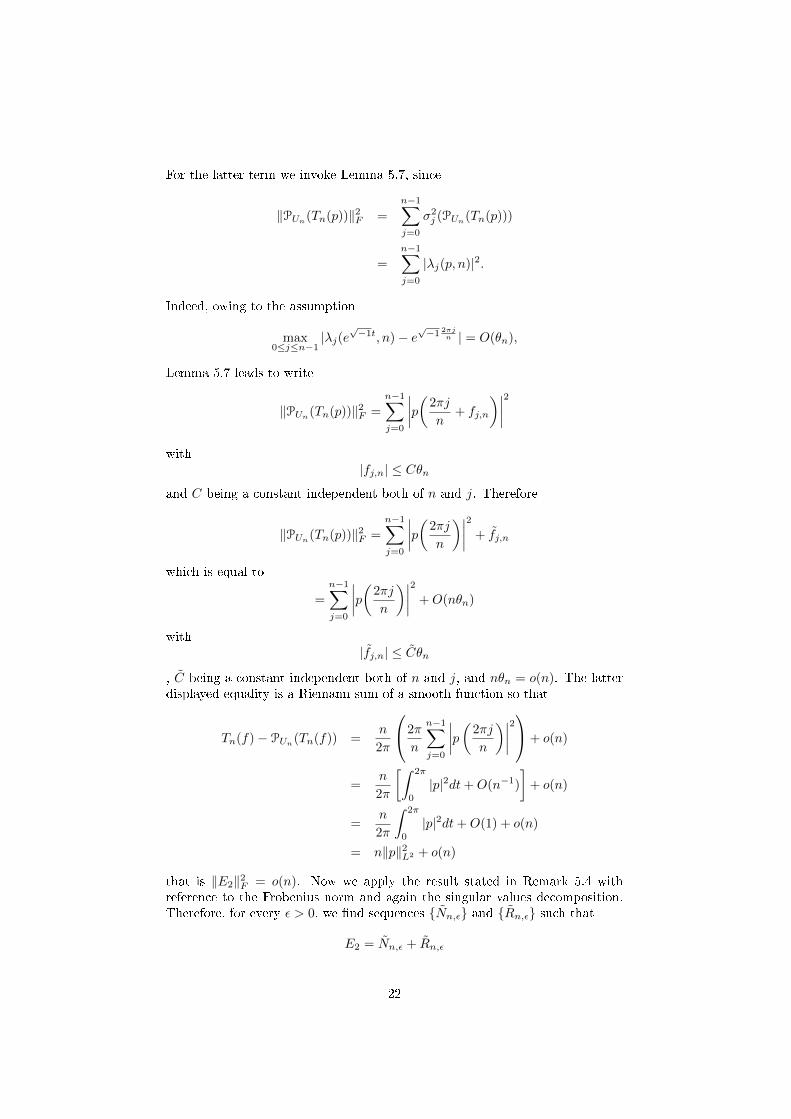
For the latter term we invoke Lemma 5.7, since

‖PUn(Tn(p))‖2F =

n−1∑j=0

σ2j (PUn(Tn(p)))

=

n−1∑j=0

|λj(p, n)|2.

Indeed, owing to the assumption

max0≤j≤n−1

|λj(e√−1t, n)− e

√−1 2πj

n | = O(θn),

Lemma 5.7 leads to write


n−1∑j=0

∣∣∣∣p(2πj

n+ fj,n

)∣∣∣∣2with

|fj,n| ≤ Cθnand C being a constant independent both of n and j. Therefore


n−1∑j=0

∣∣∣∣p(2πj

n

)∣∣∣∣2 + fj,n

which is equal to

=

n−1∑j=0

∣∣∣∣p(2πj

n

)∣∣∣∣2 +O(nθn)

with|fj,n| ≤ Cθn

, C being a constant independent both of n and j, and nθn = o(n). The latterdisplayed equality is a Riemann sum of a smooth function so that

Tn(f)− PUn(Tn(f)) =n

2π

2π

n

n−1∑j=0

∣∣∣∣p(2πj

n

)∣∣∣∣2+ o(n)

=n

2π

[∫ 2π

0

|p|2dt+O(n−1)

]+ o(n)

=n

2π

∫ 2π

0

|p|2dt+O(1) + o(n)

= n‖p‖2L2 + o(n)

that is ‖E2‖2F = o(n). Now we apply the result stated in Remark 5.4 withreference to the Frobenius norm and again the singular values decomposition.Therefore, for every ε > 0, we nd sequences Nn,ε and Rn,ε such that

E2 = Nn,ε + Rn,ε

22

‖Nn,ε‖ < ε/3 and rank(Rn,ε) ≤ r(ε)n with

limε→0

r(ε) = 0.

Finally we choose δ = ε/3 and the proof is concluded with reference to (14) andwith the equalities

Rn,ε = Rn,ε, Nn,ε = Nn,ε + E1 + E3.

•We follow the same proof given in Theorem 5.8. In particular, in all the

relevant equations the terms o(n) are replaced by terms of constant order. Inthe following we give all the proof for the sake of completeness. (Notice that in[25], the proof is given under a more general assumption that the grid pointsconsidered in Lemma 5.7 enjoy a property of quasi-uniform distribution, whenthe weak clustering of Tn(f)−PUn(Tn(f)) is derived, or a property of uniformdistribution, when the strong clustering of Tn(f)− PUn(Tn(f)) is obtained.)



n , j = 0, . . . , n − 1, and let us take the se-quence Φn of linear positive operators from C2π in itself, dened via the lineareigenvalue functionals in (13). If

maxi=0,...,n−1

‖λj(e√−1x, n)− e

√−1x

(n)j ‖∞ = O(θn),

with θn = O(n−1), for n going to innity, then for every f ∈ C2π the sequenceTn(f)− PUn(Tn(f)) in clustered at zero.

Proof In analogy with the previous theorem, by denition of strong clus-tering and taking into consideration the singular value decomposition, givenf ∈ C2π, the thesis amounts in proving that, for every ε > 0, there exist se-quences Nn,ε and Rn,ε such that


with ‖Nn,ε‖ < ε and rank(Rn,ε) ≤ r(ε).We take a generic function f ∈ C2π. By virtue of the second Weierstrass

theorem (i.e. Theorem 1.2 with N = 1), for every δ > 0 there exists pδ forwhich

‖f − pδ‖∞ < δ





= E1 + E2 + E3,

where E1 = Tn(f − pδ), E2 = Tn(pδ)−PUn(Tn(pδ)), E3 = PUn(Tn(Pδ − f)) arethe error terms. At this point, we observe that relations (9) and (11) implies

‖E1‖ ≤ ‖f − pδ‖∞ < δ

23

, while the previous inequality and Item 6 in Lemma 5.5, with the choice of thespectral norm, leads to

‖E3‖ ≤ ‖E1‖ < δ.

Now we must prove handle the term E2 and for it we consider the Frobeniusnorm, having in mind both Lemma 5.3 and Item 5 in Lemma 5.5 (the Pythagoraequality). In fact


with

p(t) = pδ(t) =

q∑j=−q

aje√−1jt.

Now looking at the entries of the Toeplitz matrix Tn(p) generated by the poly-nomial p = pδ, we have (n− 2q)‖p‖2L2 ≤ ‖Tn(p)‖2F ≤ n‖p‖2L2 since

q∑j=−q

|aj |2 = ‖p‖2L2 .





n−1∑j=0

σ2j (PUn(Tn(p)))

=

n−1∑j=0

|λj(p, n)|2.


max0≤j≤n−1

|λj(e√−1t, n)− e

√−1 2πj

n | = O(n−1),



n−1∑j=0

∣∣∣∣p(2πj

n+ fj,n

)∣∣∣∣2with

|fj,n| ≤C

n

and C being a constant independent both of n and j. Therefore


n−1∑j=0

∣∣∣∣p(2πj

n

)∣∣∣∣2 + fj,n

24

which is equal to

=

n−1∑j=0

∣∣∣∣p(2πj

n

)∣∣∣∣2 +O(1)

with

|fj,n| ≤C

n

and C being a constant independent both of n and j. The latter displayedequality is a Riemann sum of a smooth function so that


2π

2π

n

n−1∑j=0

∣∣∣∣p(2πj

n

)∣∣∣∣2+O(1)

=n

2π

[∫ 2π

0

|p|2dt+O(n−1)

]+O(1)

=n

2π

∫ 2π

0

|p|2dt+O(1)

= n‖p‖2L2 +O(1)

that is ‖E2‖2F = O(1). Furthermore the application of Lemma 5.3 with theFrobenius norm, in connection with the use of the singular value decomposition,implies that for every ε > 0, we nd sequences Nn,ε and Rn,ε such that

E2 = Nn,ε + Rn,ε

‖Nn,ε‖ < ε/3 and rank(Rn,ε) ≤ r(ε). Finally we choose δ = ε/3 and the proofis concluded with reference to (15) and with the equalities

Rn,ε = Rn,ε, Nn,ε = Nn,ε + E1 + E3.

•



n , j = 0, . . . , n−1, and let us take the sequenceΦn of linear positive operators from C2π in itself, dened via the linear eigen-value functionals in (13). If

maxi=0,...,n−1

‖λj(e√−1x, n)− e

√−1x

(n)j ‖∞ = O(θn),

with θn tending to zero, as n tends to innity, then for every f ∈ L1(0, 2π) thesequence Tn(f)− PUn(Tn(f)) is weakly clustered at zero.

Proof By denition of clustering (see Denition 5.1) and taking into con-sideration the singular value decomposition, see [14], given f ∈ C2π, the thesisamounts in proving that, for every ε > 0, there exist sequences Nn,ε andRn,ε such that


with ‖Nn,ε‖ < ε and rank(Rn,ε) ≤ r(ε)n with

limε→0

r(ε) = 0.

25

We take a generic function f ∈ L1(0, 2π). By virtue of the density of trigono-metric polynomials in the space L1(0, 2π), in the L1 topology, for every δ > 0there exists pδ for which

‖f − pδ‖L1 < δ





= E1 + E2 + E3,

where E1 = Tn(f − pδ), E2 = Tn(pδ)−PUn(Tn(pδ)), E3 = PUn(Tn(Pδ − f)) arethe error terms. At this point we invoke a variational characterization in [28]which leads to the inequality

‖E1‖S,1 ≤ ‖f − pδ‖∞ < δn

, while the previous inequality and Item 6 in Lemma 5.5, with the choice of theSchatten 1-norm, leads to

‖E3‖S,1 ≤ ‖E1‖S,1 < δn.

Therefore, by applying result stated in Remark 5.4 with the Schatten 1-normand by recalling the singular value decomposition, we nd sequences Nn,δ andRn,δ such that

E1 + E3 = Nn,δ + Rn,δ

‖Nn,δ‖ <√δ and rank(Rn,ε) ≤

√δn.

Now we must prove handle the term E2 and for it we consider the Frobeniusnorm, having in mind both Remark 5.4 and Item 5 in Lemma 5.5 (the Pythagoraequality). In fact


with

p(t) = pδ(t) =

q∑j=−q

aje√−1jt.

By looking at the entries of the Toeplitz matrix Tn(p) generated by the polyno-mial p = pδ, we have (n− 2q)‖p‖2L2 ≤ ‖Tn(p)‖2F ≤ n‖p‖2L2 since

q∑j=−q

|aj |2 = ‖p‖2L2 .



26



n−1∑j=0

σ2j (PUn(Tn(p)))

=

n−1∑j=0

|λj(p, n)|2.


max0≤j≤n−1

|λj(e√−1t, n)− e

√−1 2πj

n | = O(θn),



n−1∑j=0

∣∣∣∣p(2πj

n+ fj,n

)∣∣∣∣2with

|fj,n| ≤ Cθnand C being a constant independent both of n and j. Therefore


n−1∑j=0

∣∣∣∣p(2πj

n

)∣∣∣∣2 + fj,n

which is equal to

=

n−1∑j=0

∣∣∣∣p(2πj

n

)∣∣∣∣2 +O(nθn)

with|fj,n| ≤ Cθn

, C being a constant independent both of n and j, and nθn = o(n). The latterdisplayed equality is a Riemann sum of a smooth function so that


2π

2π

n

n−1∑j=0

∣∣∣∣p(2πj

n

)∣∣∣∣2+ o(n)

=n

2π

[∫ 2π

0

|p|2dt+O(n−1)

]+ o(n)

=n

2π

∫ 2π

0

|p|2dt+O(1) + o(n)

= n‖p‖2L2 + o(n)

that is ‖E2‖2F = o(n). Now we apply the result stated in Remark 5.4, withreference to the Frobenius norm, and again the singular values decomposition.Therefore, for every ε > 0, we nd sequences Nn,ε and Rn,ε such that

E2 = Nn,ε + Rn,ε

27

‖Nn,ε‖ < ε/2 and rank(Rn,ε) ≤ r(ε)n with

limε→0

r(ε) = 0.

Finally we choose δ = ε2/4 and the proof is concluded with reference to (16)and with the equalities

Rn,ε = Rn,ε2/4 + Rn,ε, Nn,ε = Nn,ε2/4 + Nn,ε.

•

Remark 5.11. We may notice that it is not necessary to know the functionf to construct the continuous linear operator, but only its Fourier coecients,which in turn can be numerically evaluated in a stable a fast way by using the(discrete) fast Fourier transform (see [13]).

5.3.1 The check of the Korovkin test in the matrix Toeplitz setting

Let us follow Theorem 5.9 and let us consider rst the most popular choice ofthe sequence Un that is the case where Un is the discrete Fourier matrix Fn[35] with

Fn =(e−√−1 2πjk

n

)n−1

j,k=0.

In that case the related algebra A(Fn) (in the sense of Section 5.2) is the algebraof circulants [9, 13] in which X ∈ A(Fn) if and only if

X =(b(j−k) mod n

)n−1

j,k=0

for some complex coecients b0, . . . , bn−1 where

X = FnD(X)F ∗n , [D(X)]j,j = pb

(2πj

n

), pb(t) =

n−1∑k=0

bke√−1kt.

In this case the minimization in the Frobenius norm is very easy because theproblem decouples into n distinct one-variable minimization problems. In par-

ticular if T =(a(j−k)

)n−1

j,k=0is of Toeplitz type then

minX∈A(Fn)

‖TX‖2F = minb0,...,bn−1∈C

n−1∑k=0

|ak − bk|2(n− k) + |ak−n − bk|2k

whose optimal solution is expressible explicitly as

bk =kak−n + (n− k)ak

n. (17)

Now we are ready for the Korovkin test (see Theorem 5.9). We take g(x) =

e√−1x and the Toeplitz matrix of size n generated by g(x) that is Tn(g(x))

which is the transpose of the Jordan block of size n. In other words the (j, k)entry of Tn(g(x)) is 1 if j − k = 1 and is zero otherwise. According to formula

28

(17) we have b1 = 1− 1/n and bk = 0 for k 6= 1. Therefore the j-th eigenvalueof the optimal approximant is

λj(e√−1x, n) =

(F ∗nTn(e

√−1x)Fn

)j,j

= (1− 1/n)e√−1 2πj

n .

As a consequence

maxij=0,...,n−1

‖λj(e√−1x, n)− e

√−1x

(n)j ‖∞ = n−1

with x(n)j = 2πj

n and the crucial assumption of Theorem 5.9 is fullled. Thereforewe conclude that the sequence Tn(f) − PUn(Tn(f)) is clustered at zero, forevery f ∈ C2π and weakly clustered at zero for every f ∈ L1(0, 2π).

In the literature we nd many sequences of matrix algebras associated tofast transforms. The Korovkin test was performed originally for the circulantsand all ω-circulants with |ω| = 1 in [25]. The test in the case of all known sineand cosine algebras was veried in [10], while the case all Hartley transformspaces was treated in detail in [2]. It should be observed that the extension tothe case of multilevel block structures (see [26]) is not dicult, as mentionedand briey sketched in the next subsection.

5.3.2 The multilevel case

By following the notations of Tyrtyshnikov, a multilevel Toeplitz matrix oflevel N and dimension n1 × n2 × · · · × nN is dened as the matrix generatedby the Fourier coecients of a multivariate Lebesgue integrable function f =f(x1, . . . , xN ) according to the law given in equations (6.1) at page 23 of [32](see also [31]). In the following, for the sake of readability, we shall often writen for the N -tuple (n1, . . . , nN ), n = n1 · · ·nN . Then, for f ∈ L1((0, 2π)N ) beingN -variate and taking values into the rectangular matrices Ms,t(C), we denethe sn× tn multilevel Toeplitz matrix by

Tn(f) =

n1−1∑j1=−n1+1

· · ·nN−1∑

jN=−nN+1

J (j1)n1⊗ · · · ⊗ J (jN )

nN ⊗ a(j1,...,jN )(f), (18)

where⊗ denotes the tensor or Kronecker product of matrices and J(`)m , (−m+1 ≤

` ≤ m−1, is them×mmatrix whose (i, j)th entry is 1 if i−j = ` and 0 otherwise;thus J−m+1, . . . , Jm−1 is the natural basis for the space of m × m Toeplitzmatrices. In the usual multilevel indexing language, we say that [Tn(f)]r,j =aj−rwhere (1, . . . , 1) ≤ j, r ≤ n = (n1, . . . , nN ), i.e., 1 ≤ j` ≤ n` for 1 ≤ ` ≤ N andthe j-th Fourier coecient of f that is

aj =1

(2π)N

∫[0,2π]N

f(t)e−√−1(j1t1+···+jN tN ) dt,

J = (j1, . . . , jN ), is a rectangular matrix of size s × t. The latter relation to-gether with (18) denes a sequence Tn(·) of operators, Tn : L1((0, 2π)N ) →Msn,tn(C), which are clearly linear, due to the linearity of the Fourier coe-cients, and positive in a sense specied in [26]. Similarly, given the unitary

29

matrix Un related to the transform of a one-level algebra, a corresponding N -level algebra is dened as the set of n1× n2× · · · × nN matrices simultaneouslydiagonalized by means of the following tensor product of matrices

Un = Un1⊗ Un2

⊗ · · · ⊗ UnN , (19)

with A ⊗ B being the matrix formed in block form as (Ai,jB). Now, sincewe are interested in extending the results proved in the preceding sections tom dimensions, we analyze what is necessary to have and, especially, what iskept when we switch from one dimension to m dimensions: for the rst levelwe used the Weierstrass and Korovkin Theorems, the last part of Lemma 5.5,Lemma 5.3 and Remark 5.4. Surprisingly enough, we nd that all these toolshold or have a version in N dimensions: for the Korovkin and the WeierstrassTheorems, the multidimensional extensions are classic results, while Lemma5.3 and Remark 5.4 contain statements not depending on the structure of thematrices and Lemma 5.5 is valid for any algebra and so for multilevel algebrasas well (recall that Un in (19) is unitary).

Therefore, we instantly deduce the validity in m dimensions of the mainstatements of this paper that is Theorems 5.8, 5.9, 5.9. However, we remarkthat we have no examples in which the strong convergence holds.

For instance, in the two-level circulant and τ cases, only the weak conver-gence has been proved because the number of the outliers is, in both cases,equal to O(n1 + n2) [6, 11] even if the function f is a bivariate polynomial:more precisely, this means that the hypotheses of Theorem 5.9, regarding thestrong approximation in the polynomial case, are not fullled by the two-levelcirculant and τ algebras and therefore strong convergence cannot be proved inthe general case (see also [26]). Very recently, in [29] and [30] it has been provedthat any sequence of preconditioners belonging to Partially Equimodular al-gebras [30] cannot be superlinear for sequence of multilevel Toeplitz matricesgenerated by simple positive polynomials. Here, Partially Equimodular refersto some very weak assumptions on Un that are instanly fullled by all the knownmultilevel trigonometric algebras.

6 Concluding Remarks

In these notes, we have shown classical applications of the Korovkin theory tothe approximation of functions. A new view on the potential of the Korovkintheorems is provided in a context of Numerical Linear Algebra. Here the mainnovelty is that the poor approximation from a quantitative viewpoint (see Ex-ercise 3) is not a limitation. In reality, when employing preconditioned Krylovmethods for the solution of large linear system, only a modest quantitative ap-proximation of the spectrum is required in order to design optimal iterativesolvers (see [12] and [4] for the specic commection between the spectrum ofthe preconditioned matrices and the iteration count of the associated iterativemethod).

7 Appendix A: General Tools

Linear and positives operators properties are necessary to prove the KorovkinTheorem. Therefore we consider following Lemma. It shows that the monotony

30

is obtained by properties linearity and positivity.

Lemma 7.1. Let A and B be vector spaces both endowed with a partial orderingand let Φ : A → B be a linear and positive operator. Then Φ is monotone thatis, if f and g are elements of A with f ≥ g we necessarily have Φ(f) ≥ Φ(g).

Proof By the assumption f ≥ g we nd

f − g ≥ 0A.

then, using the positivity of the operator Φ we have

Φ(f − g) ≥ Φ(0A) = 0B.

Finally by linearity we obtain Φ(f)− Φ(g) ≥ 0B which in turn leads to

Φ(f) ≥ Φ(g).

2

As a direct consequence of the above lemma we get the isotonic property, atleast if f = f∗. In fact if our spaces are equipped with the modulus we have

±f ≤ |f |

and therefore the monotonicity implies

±Φ(f) ≤ Φ(|f |)⇔ |Φ(f)| ≤ Φ(|f |).

The latter is known as isotonic property. However not all vectorial spaces havea modulus, for example a modulus is not dened for linear space generated bythe test functions in Theorem 3.1.

Example: A well known example of isotonic functional is the integral denedin the space of complex valued integrable functions (L1[a, b]). In fact for f ∈L1[a, b] we know that ∣∣∣∫ b

af(x)dx

∣∣∣ ≤ ∫ b

a

|f(x)|dx.

Concerning generalized versions of the isotonic property the reader is referred to[28], where, in the context of general matrix valued linear positive operators, itis proved that |‖Φn(f)‖| ≤ |‖Φn(|f |)‖| for every f ∈ Lp(Ω), p ≥ 1, Ω equippedwith a σ-nite measure, for every matrix valued linear positive operator Φn(·),n ≥ 1, from Lp(Ω) to Mn(C), for every unitarily invariant norm. The space Lp

can be replaced by C(K) for some compact set K in RN , N ≥ 1, thanks to theRadon-Nykodim theorem (see [21]).

8 Appendix B: the (algebraic) Korovkin theoremin N dimensions

We now give a full proof of the Korovkin theorem in N dimensions. Concerningnotation we recall that the symbol ‖ · ‖2 indicates the Euclidean norm over CN

that is ‖x‖2 =(∑N

i=1 |xi|2)1/2

for x ∈ CN .

31

Theorem 8.1 (Korovkin). Let K be a compact set of RN and let us considerthe standard Banach space C(K) endowed the sup-norm. Let us denote byT = 1, xi, ‖x‖22 : i = 1, . . . , N the standard Korovkin set of test functions andlet us take a sequence Φn of linear positive operators from C(K) in itself. Iffor any g ∈ T

Φn(g) uniformly converges to g

then Φn is an approximation process i.e.

Φn(f) uniformly converges to f, ∀f ∈ C(K).

Proof We set f ∈ C(K), we take an arbitrary ε > 0 and we show that thereexists n large enough for which ‖f − Φn(f)‖∞,K ≤ ε, for every n ≥ n. Hencewe take any point x of K and we consider the dierence

f(x)− Φn(f(y))(x)

where y is the dummy variable inside the operator Φn, where the function facts. We now observe that the constant function 1 belongs to the Korovkintest set T and therefore 1 = (Φn(1))(x) − εn(1)(x), where εn(1) uniformlyconverges to zero over K. As a consequence, the use of the linearity of any Φnleads to

f(x)− Φn(f(y))(x) = [Φn(1)(x)− εn(1)(x)]f(x)− Φn(f(y))(x)

= Φn(f(x)− f(y))(x)− εn(1)(x)f(x).

Thus there exists a value n1 such that for every n ≥ n1 we nd

|εn(1)(x)f(x)| ≤ ‖εn(1)‖∞,K‖f‖∞,K ≤ ε/4.

By exploiting the linearity and positivity of Φn (see Appendix A), we obtain

|f(x)− Φn(f(y))(x)| ≤ |Φn(f(x)− f(y))(x)|+ ε/4 (20)

≤ Φn(|f(x)− f(y)|)(x) + ε/4.

As in the one-dimensional case the remaining part of the proof consists in a clevermanipulation of the term |f(x) − f(y)|, of which we look for a sharp upper-bound, with the underlying idea of exploiting both the linearity and positivity ofthe operators and the assumption of convergence on the Korovkin test functions.

For manipulating the quantity |f(x)− f(y)| we use the denition of uniformcontinuity. We are allowed to assume f uniformly continuous, since the notionsof continuity and uniform continuity are the same when the function is denedon a compact set. Therefore for every ε1 > 0, there exists δ > 0 such that‖x− y‖2 ≤ δ implies |f(x)− f(y)| ≤ ε1. Now, depending on the new parameterδ (and then in correspondence to the behavior of our function f), we dene thepair of sets

Qδ = y ∈ K : ‖x− y‖2 ≤ δ, QCδ = K\Qδ.

We observe that |f(x)−f(y)| is bounded from above by ε1 onQδ and by 2‖f‖∞,Ksu QCδ , thanks to the triangle inequality. We denote by χJ the characteristicfunction of the set J. Therefore the observation that x, y ∈ QCδ implies ‖x−y‖2 >δ leads to

1 ≤ ‖x− y‖22/δ2,

32

for x, y ∈ QCδ . As a consequence we deduce the following chain of relationships.

|f(x)− f(y)| ≤ ε1χQδ(y) + 2‖f‖∞,KχQCδ (y)

≤ ε1χQδ(y) + 2‖f‖∞,KχQCδ (y)‖x− y‖22/δ2

≤ ε1 + 2‖f‖∞,K‖x− y‖22/δ2.

The use of the positivity of Φn allows one to conclude

Φn(|f(x)− f(y)|) ≤ Φn(ε1 + 2‖f‖∞,K‖x− y‖22/δ2

).

Finally, using the linearity of Φn and setting ∆n(f)(x) = |f(x)−Φn(f(y))(x)|,from (20) we infer the concluding relations, that is

∆n(f)(x) ≤ Φn(|f(x)− f(y)|)(x) + ε/4

≤ Φn(ε1 + 2‖f‖∞,K‖x− y‖22/δ2

)(x) + ε/4

= ε1Φn(1)(x) + 2‖f‖∞,K/δ2Φn(‖x− y‖22

)(x) + ε/4

= ε1Φn(1)(x) + 2‖f‖∞,K/δ2

Φn

(N∑i=1

x2i − 2xiyi + y2

i

)(x) + ε/4

= ε1Φn(1)(x) + 2‖f‖∞,K/δ2

N∑i=1

Φn(x2i − 2xiyi + y2

i

)(x) + ε/4

= ε1Φn(1)(x) + 2‖f‖∞,K/δ2

N∑i=1

[x2iΦn(1)(x)− 2xiΦn(yi)(x) + Φn(y2

i )(x)]

+ ε/4

= ε1Φn(1)(x) + 2‖f‖∞,K/δ2[N∑i=1

[x2iΦn(1)(x)− 2xiΦn(yi)(x)

]+ Φn(‖y‖22)(x)

]+ε/4.

We have now reduced the argument of Φn to a linear combination of testfunctions. Therefore we can proceed with explicit computations: setting Φn(g) =g + εn(g), with εn(g) uniformly converging to zero over K, we have

∆n(f)(x) ≤ ε1(1 + εn(1)(x)) + 2‖f‖∞,K/δ2[N∑i=1

[x2iΦn(1)(x)− 2xiΦn(yi)(x)

]+ Φn(‖y‖22)(x)

]+ ε/4

= ε1(1 + εn(1)(x)) + 2‖f‖∞,K/δ2[N∑i=1

[x2i εn(1)(x)− 2xiεn(yi)(x)

]+ εn(‖y‖22)(x)

]+ ε/4.

Finally, due to the uniform convergence to zero of the error functions εn(g),we deduce that there exists a value n ≥ n1 for which, for every n ≥ n we nd

33

εn(1))(x) ≤ 1 and

2‖f‖∞,K/δ2

[N∑i=1

[x2i εn(1)(x)− 2xiεn(yi)(x)

]+ εn(‖y‖22)(x)

]≤ ε/4.

In conclusion, by combining the partial results and by choosing properly ε1 asa function of ε, we have proven the thesis namely

∆n(f)(x) = |f(x)− Φn(f(y))(x)| ≤ ε, ∀n ≥ n.

•

9 Appendix C: the (periodic) Korovkin theoremin N dimensions

We now give a full proof of the Korovkin theorem in N dimensions in the 2πperiodic case. We consider the Banach space

C2π = f : RN → C, f continuous and periodic i.e. f(x) = f(x mod 2π)

endowed with the sup-norm. The only substantial change will be in the set oftest functions and in a clever variation of the notion of uniform continuity.

Theorem 9.1 (Korovkin). Let us consider the standard Banach space C2π en-

dowed the sup-norm. Let us denote by T = 1, e√−1xi : i = 1, . . . , N the

standard Korovkin set of 2π periodic test functions and let us take a sequenceΦn of linear positive operators from C2π in itself. If for any g ∈ T

Φn(g) uniformly converges to g

then Φn is an approximation process i.e.

Φn(f) uniformly converges to f, ∀f ∈ C2π.

Proof. We x f ∈ C2π, we take an arbitrary ε > 0 and we show that thereexists n large enough for which ‖f − Φn(f)‖∞,K ≤ ε, for every n ≥ n. Hencewe take any point x of K and we consider the dierence

f(x)− Φn(f(y))(x)

where y is the dummy variable inside the operator Φn, where the function facts. We now observe that the constant function 1 belongs to the Korovkin testset T and therefore 1 = Φn(1)(x)− εn(1)(x), where εn(1) uniformly convergesto zero over K. As a consequence, the use of the linearity of any Φn leads to

f(x)− Φn(f(y))(x) = [Φn(1)(x)− εn(1)(x)]f(x)− Φn(f(y))(x)

= Φn(f(x)− f(y))(x)− εn(1)(x)f(x).

Thus there exists a value n1 such that for every n ≥ n1 we nd

|εn(1)(x)f(x)| ≤ ‖εn(1)‖∞,K‖f‖∞,K ≤ ε/4.

34

By exploiting the linearity and positivity of Φn (see Appendix A), we obtain

|f(x)− Φn(f(y))(x)| ≤ |Φn(f(x)− f(y))(x)|+ ε/4 (21)

≤ Φn(|f(x)− f(y)|)(x) + ε/4.

As in Theorem 8.1, the remaining part of the proof consists in a clever manip-ulation of the term |f(x) − f(y)|, of which we look for a sharp upper-bound,with the underlying idea of exploiting both the linearity and positivity of theoperators and the assumption of convergence on the Korovkin test functions.

For manipulating the quantity |f(x)− f(y)| we use the denition of uniformcontinuity. We are allowed to assume f uniformly continuous, since the notionsof continuity and uniform continuity are the same when the function is denedon a compact set and the set RN can be reduced to the compact set [0, 2π]N

thanks to the 2π-periodicity considered in the assumptions. Therefore for everyε1 > 0, there exists δ > 0 such that ‖z(x)−z(y)‖2 ≤ δ implies |f(x)−f(y)| ≤ ε1with

[z(x)]i = e√−1xi , i = 1, . . . , N.

Now, depending on the new parameter δ (and then in correspondence to thebehavior of our function f), we dene the pair of sets

Qδ = y ∈ RN : ‖z(x)− z(y)‖2 ≤ δ, QCδ = RN\Qδ.

We observe that |f(x) − f(y)| is bounded from above by ε1 on Qδ and by2‖f‖∞,RN su QCδ , thanks to the triangle inequality. We denote by χJ the char-acteristic function of the set J. Therefore the observation that x, y ∈ QCδ implies‖z(x)− z(y)‖2 > δ leads to

1 ≤ ‖z(x)− z(y)‖22/δ2,

for x, y ∈ QCδ . As a consequence we deduce the following chain of relationships.

|f(x)− f(y)| ≤ ε1χQδ(y) + 2‖f‖∞,RNχQCδ (y)

≤ ε1χQδ(y) + 2‖f‖∞,RNχQCδ (y)‖z(x)− z(y)‖22/δ2

≤ ε1 + 2‖f‖∞,RN ‖z(x)− z(y)‖22/δ2.

The use of the positivity of Φn allows one to conclude

Φn(|f(x)− f(y)|) ≤ Φn(ε1 + 2‖f‖∞,RN ‖z(x)− z(y)‖22/δ2

).

Finally, using the linearity of Φn and setting ∆n(f)(x) = |f(x)−Φn(f(y))(x)|,

35

from (21) we infer the concluding relations, that is

∆n(f)(x) ≤ Φn(|f(x)− f(y)|)(x) + ε/4

≤ Φn(ε1 + 2‖f‖∞,RN ‖z(x)− z(y)‖22/δ2

)(x) + ε/4

= ε1Φn(1)(x) + 2‖f‖∞,RN /δ2Φn(‖z(x)− z(y)‖22

)(x) + ε/4

= ε1Φn(1)(x) + 2‖f‖∞,RN /δ2

Φn

(N∑i=1

1− e−√−1xie

√−1yi − e

√−1xie−

√−1yi + 1

)(x) + ε/4

= ε1Φn(1)(x) + 2‖f‖∞,RN /δ2

N∑i=1

Φn

(2− e−

√−1xie

√−1yi − e

√−1xie−

√−1yi

)(x) + ε/4

= ε1Φn(1)(x) + 2‖f‖∞,RN /δ2

N∑i=1

[Φn(2)(x)− [z(x)]iΦn([z(y)]i)(x)− [z(x)]iΦn([z(y)]i)(x)

]+

+ε/4.

We have now reduced the argument of Φn to a linear combination of testfunctions. Therefore we can proceed with explicit computations: setting Φn(g) =g + εn(g), with εn(g) uniformly converging to zero over K, we obtain that∆n(f)(x) is bounded from above by

ε1(1 + εn(1)(x)) + 2‖f‖∞,RN /δ2 ·

·

[N∑i=1

[2εn(1)(x)− [z(x)]iεn([z(y)]i)(x)− [z(x)]iεn([z(y)]i)(x)

]]+

+ε/4.

Finally, due to the uniform convergence to zero of the error functions εn(g),we deduce that there exists a value n ≥ n1 for which, for every n ≥ n we ndεn(1)(x)) ≤ 1 and the quantity

2‖f‖∞,RN /δ2

[N∑i=1

2εn(1)(x)− [z(x)]iεn([z(y)]i)(x)− [z(x)]iεn([z(y)]i)(x)

]

globally bounded from above by ε/4. In conclusion, by combining the partialresults and by choosing properly ε1 as a function of ε, we have proven the thesisnamely

∆n(f)(x) = |f(x)− Φn(f(y))(x)| ≤ ε, ∀n ≥ n.

•

10 Exercises

1. With reference to the notations of Section 4.3 complete the proof of theWeierstrass Theorem by using the Gauss-Weierstrass operators.

36

2. Let Φn be a sequence of linear positive operators from C[0, 1] into it-self such that Φn(g(t))(x) = g(x) for all x ∈ [0, 1], for all standard testfunctions g(t) = tj , j = 0, 1, 2. Prove that the sequence is trivial i.e.Φn(f) ≡ f for every f ∈ C[0, 1]. (Compare this result with the case ofinterpolation operators: conclude that interpolation operators, which arelinear, cannot be positive).

3. Let Φn be a sequence of linear positive operators such that Φn acts onC[0, 1], Φn(f) is a polynomial of degree at most n for every f ∈ C[0, 1]and such that the innity norm of n2(Φn(g(t))(x)− g(x)) goes to zero asn tends to innity, for all standard test functions g(t) = tj , j = 0, 1, 2.Prove that such a sequence cannot exist. Hint: for that exercise a goodstarting point is the following saturation result. Let f ∈ Ck[0, 1] for somek ≥ 0 and let

En(f) = minp∈Pn

‖f − p‖∞,[0,1].

Then for every k ≥ 0, for every non-increasing, nonnegative sequence εntending to zero as n tends to innity, there exists f ∈ Ck[0, 1] such that

En(f)nk ≥ εn.

(Compare this result with the case of interpolation operators and espe-cially with the Faber Theorem [33] and Jackson estimates [16, 19]: in-terpolation operators do not guarantee convergence for every continuousfunction f , but could be extremely fast convergent if f is smoother).

4. Give a (constructive) proof of the saturation theorems stated in the pre-vious exercise: start with the case k = 0.

5. With reference to the notations of Section 4.3, consider the sentence theproof is only partially constructive since pn,m is dened using informationon f not available in general (except via numerical evaluations) given inthe last part of the section: identify this information.

6. Prove the multiplicative separability property for the Bernstein operatorsi.e.

Bn(f(t))(x) = Bn(g(t))(x)Bn(h(t))(x)

whenever f(t) = g(t)h(t) with

n = (n1, . . . , nN ),

t = (t1, . . . , tN ),

x = (x1, . . . , xN ),

v = (vi1 , . . . , iq), 1 ≤ i1 < · · · < iq ≤ N,v = (vj1 , . . . , jr), 1 ≤ j1 < · · · < jr ≤ N,

q + r = N,

i1, . . . , iq ∪ j1, . . . , jr = 1, . . . , N.

7. Verify the multidimensional Korovkin test for multidimensional Bernsteinoperators (use the multiplicative separability property of the previous ex-ercise and reduce the multidimensional case to the unidimensional casealready treated in Section 4.1).

37

8. Prove the Korovkin Theorem by varying some ingredients

a Following the proof of Theorem 9.1, prove:

Φn(g) converges in L1 norm to g, ∀g ∈ T

then the sequence Φn of LPOs is an approximation process namely

Φn(f) converges in L1 norm to f, ∀f ∈ C2π.

b Give the Korovkin test set in the case periodic and real.

c Give the Korovkin test set in the case periodic, real, and even i.e.f(−x) = f(x), x ∈ [0, π].

d With reference to the previous items give the Korovkin test set in themultidimensional setting.

9. For f ∈ L1(−π, π) let Cn(f)(x) = 1n+1

∑nk=0 Fk(f)(x) be its Cesaro sum

of degree n with Fk(f)(x) =∑kj=−k aje

√−1jx, being its k-th Fourier sum

and aj = aj(f) being its j-th Fourier coecient. Let Tn(f) be the (n +1)× (n+ 1) Toeplitz matrix dened as

Tn(f) = (as−t)ns,t=0 .

and v(x) be the vector of length n+ 1 with k-th entry given by e−√−1kx.

[a] Prove the identity Cn(f)(x) = 1n+1v

∗(x)Tn(f)v(x).

[b] We already proved that Tn(·) : L1(−π, π)→Mn(C) is a LPO. Usingthe latter prove that Cn(·) : L1(−π, π)→ L1(−π, π) is a LPO.[c] Assuming that f ∈ L∞(−π, π) and that f is real-valued, prove thatCn(f)(x) ≥ ess inf f and Cn(f)(x) ≤ ess sup f , ∀x ∈ [−π, π] (if you prefer,assume that f ∈ C2π).[d] By using the right Korovkin theorem prove that ∀f ∈ C2π

limn→∞

‖Cn(f)(x)− f(x)‖∞ = 0.

Notice that the latter furnishes a constructive proof of the second Weier-strass Theorem (see Theorem 1.2).[e] From the monumental book of Zygmund on Trigonometric Series [39]we learn that the k-th Cesaro sum is such that

Ck(f)(x) = f(x) +s(f)(x)

k + 1+ rk(f)(x) (22)

where f is smooth enough, s(f)(x) is a bounded function independent of k,and ‖rk(f)(x)‖∞ is of the order of the best trigonometric approximationof degree k, for k →∞. Suppose that one has computed g1 = Cn−1(f)(x)and g2 = C3n−1(f)(x) for some suciently large value of n. How toexploit (22) in order to compute f(x) within an error of the order of‖rn−1(f)(x)‖∞?[f ] Show that Cn(2− 2 cos(t))(0) ∼ n−1 by direct computation.

We set h(t) = (et2 − 1)(3 + sign(|t| − 1)| sin(t+ 1)|5/π), t ∈ (−π, π].

Is it true that Cn(h(t))(0) ∼ n−1?Is it true that Cn(hα(t))(0) ∼ n−1 for α ∈ (1, 2]?Is it true that Cn(hα(t))(0) ∼ n−1 for every xed α?

38

10. Prove all Korovkin results discussed so far, namely Theorems 8.1, 9.1, andLemma 5.6, by using the size depending norms

‖f‖∞,Jn = supx∈Jn

|f(x),

where Jn ⊂ K, K compact, in the algebraic case and Jn mod 2π · e ⊂[0, 2π)N , N ≥ 1, in the periodic case with e being the N dimensionalvector of all ones and with x ∈ Jn mod 2π · e if xj , j = 1, . . . , N , is ofthe form yj mod 2π and y ∈ Jn. The above generalization was used in[25, 26]; refer to [1] for a monumental survey on the Korovkin theory.

11. With reference to Lemma 5.6 prove that the same statement holds trueif G is the linear space of the continuous even periodic functions, if p isan even polynomial (with a nite cosine expansion) and if the Chebyshevset pii=0,1,2 is given by 1, cosx, cos 2x over I = [0, π] with Jn ⊂ I (usea similar argument and combine it with a simple technique of inductivetype).

12. Let Ω a set of Rd with d ≥ 2. Let C = g0(x), . . . , gk(x), k ≥ 1, bea collection of real-valued continuous functions over Ω. Prove that thereexist a collection of pair-wise distinct points x0, . . . , xk (i.e. xi 6= xj ifi 6= j) such that the (k + 1)× (k + 1) Vandermonde-like matrix

(gj(xk))kj,k=0

is singular whenever Ω contains a Y shaped domain (the tram switchingproof).

References

[1] F. Altomare, M. Campiti, (Appendix A by Michael Pannenberg and Ap-pendix B by Ferdinand Beckho), Korovkin-type approximation theory andits applications. de Gruyter Studies in Mathematics, 17. Walter de Gruyter,Berlin, 1994.

[2] A. Arico', S. Serra-Capizzano, M. Tasche, Fast and numerically stablealgorithms for discrete Hartley transforms and applications to precondi-tioning, Comm. Informat. Syst., 5-1 (2005), pp. 2168.

[3] O. Axelsson, V. Barker, Finite Element Solution of Boundary Value Prob-lems, Theory and Computation. Academic Press Inc., New York, 1984.

[4] O. Axelsson, G. Lindskög, The rate of convergence of the preconditionedconjugate gradient method, Numer. Math., 52 (1986), pp. 499523.

[5] R. Bhatia. Matrix Analysis. Springer-Verlag, New York, NY, 1997.

[6] R.H. Chan, X. Jin, A family of block preconditioners for block systems,SIAM J. Sci. Stat. Comput., 13 (1992), pp. 12181235.

[7] R.H. Chan, M. Ng, Conjugate gradient method for Toeplitz systems,SIAM Rev., 38 (1996), 427482.

39

[8] T.F. Chan, An optimal circulant preconditioner for Toeplitz systems,SIAM J. Sci. Stat. Comput., 9 (1988), pp. 766771.

[9] P. Davis, Circulant Matrices. John Wiley and Sons, New York, 1979.

[10] F. Di Benedetto, S. Serra-Capizzano, A unifying approach to abstractmatrix algebra preconditioning, Numer. Math., 82-1 (1999), pp. 5790.

[11] F. Di Benedetto, S. Serra-Capizzano, Optimal multilevel matrix algebraoperators, Linear Multilin. Algebra, 48 (2000), pp. 3566.

[12] F. Didone, M. Giannuzzi, L. Paulon, S. Serra-Capizzano, Solution of alarge linear system using the Preconditioned Conjugate Gradient Method.From lectures titled Approssimazione matriciale, precondizionamento esistemi lineari di grandi dimensioni by S. Serra-Capizzano in Rome, at theDepartment MeMoMat, University La Sapienza, 2010.

[13] F. Didone, M. Giannuzzi, L. Paulon, S. Serra-Capizzano, How to performa Toeplitz matrix-vector product eciently. From lectures titled Approssi-mazione matriciale, precondizionamento e sistemi lineari di grandi dimen-sioni by S. Serra-Capizzano in Rome, at the Department MeMoMat,University La Sapienza, 2010.

[14] G.H. Golub, C.F. Van Loan, Matrix Computations. The Johns HopkinsUniversity Press, Baltimore 1983.

[15] A. Greenbaum, Iterative methods for solving linear systems, SIAM publ.,Philadelphia, 1997.

[16] D. Jackson, The Theory of Approximation. American Mathematical Soci-ety, New York, 1930.

[17] P.P. Korovkin, Linear Operators and Approximation Theory (English trans-lation). Hindustan Publishing Co., Delhi, 1960.

[18] K. Kumar, N. Namboodiri, and S. Serra-Capizzano, A tutorial on the Ko-rovkin theory in approximation, (numerical) linear algebra, and operatortheory. In preparation.

[19] I.P. Natanson, Constructive Function Theory, I. Frederick Ungar Publish-ing Co., New York, 1964.

[20] M. Ng, Iterative methods for Toeplitz systems. Oxford University Press,New York, 2004. .

[21] W. Rudin, Real and Complex Analysis. McGraw-Hill, Singapore, 1986.

[22] W. Rudin, Functional Analysis. McGraw-Hill, Singapore, 1986.

[23] Y. Saad, Iterative methods for sparse linear systems. PWS Publishing,Boston, MA, 1996.

[24] S. Serra-Capizzano, Some theorems on linear positive operators and func-tionals and their applications, Comput. Math. Appl., 39-7/8 (2000), pp.139167.

40

[25] S. Serra-Capizzano, A Korovkin-type Theory for nite Toeplitz operatorsvia matrix algebras, Numer. Math., 82-1 (1999), pp. 117142.

[26] S. Serra-Capizzano, A Korovkin based approximation of multilevel Toepli-tz matrices (with rectangular unstructured blocks) via multilevel trigono-metric matrix spaces, SIAM J. Numer. Anal., 36-6 (1999), pp. 18311857.

[27] S. Serra-Capizzano Korovkin tests, approximation, and ergodic theory,Math. Comput., 69 (2000), pp. 15331558.

[28] S. Serra-Capizzano, P. Tilli, On unitarily invariant norms of matrix valuedlinear positive operators, J. Inequalities Appl., 7-3 (2002), pp. 309330.

[29] S. Serra Capizzano and E. Tyrtyshnikov, Any circulant-like preconditionerfor multilevel matrices is not superlinear, SIAM J. Matrix Anal. Appl., 21-2 (1999), pp. 431439.

[30] S. Serra-Capizzano, E. Tyrtyshnikov, How to prove that a preconditionercan not be superlinear, Math. Comput., 72-243 (2003), pp. 13051316.

[31] P. Tilli, A note on the spectral distribution of Toeplitz matrices, LinearMultilin. Algebra, 45 (1998), pp. 147159.

[32] E. Tyrtyshnikov, A unifying approach to some old and new theorems ondistribution and clustering, Linear Algebra Appl., 232 (1996), pp. 143.

[33] E. Tyrtyshnikov, A brief introduction to numerical analysis. BirkhäuserBoston, Inc., Boston, MA, 1997.

[34] E. Tyrtyshnikov, N. Zamarashkin, Spectra of multilevel Toeplitz matrices:advanced theory via simple matrix relationships, Linear Algebra Appl.,270 (1998), pp. 1527.

[35] C. Van Loan, Computational Frameworks for the Fast Fourier Transform.SIAM, Philadelphia, 1992.

[36] H. Widom, Toeplitz matrices. In Studies in real and complex analysis, I.Hirshman Jr. Ed., Math. Ass. Amer., 1965.

[37] H. Widom, Szegö limit Theorem: the higher dimensional matrix case, J.Funct. Anal., 39 (1980), pp. 182198.

[38] H. Widom, On the singular values of Toeplitz matrices, Zeit. Anal. Anw.,8 (1989), pp. 221229.

[39] A. Zygmund, Trigonometric Series. Cambridge University Press, Cam-bridge, 1959.

41

Korovkin Theorems and applications in approximation … · Korovkin Theorems and applications in...

Documents

Transcript of Korovkin Theorems and applications in approximation … · Korovkin Theorems and applications in...