Koop, Osiewalski and Steel - NYU Stern School of Business

JOURNAL OF Econometrics

ELSEVIER Journal of Econometrics 76 (1997) 77-105

Bayesian efficiency analysis through individual effects: Hospital cost frontiers

Gary K o o p a, J acek Osiewalsk i b, M a r k F.J. Steel*' c

a Department of Economics, University of Toronto, Toronto, Ont. MSS 1A1, Canada b Department of Econometrics, Academy of Economics, 31-510 KrakJw, Poland

c CentER and Department of Econometrics, Tiiburg University, 5000 LE Tilburg, The Netherlands

(Received May 1994; final version received June 1995)

Abstract

This paper develops Bayesian tools for making inferences about finn-specific inefficiencies in panel data models. We begin by establishing a Bayesian setting in which fixed and random effects models are defined. What distinguishes these classes of models is the marginal prior independence of the effects. We show how such models can be analyzed using Monte Carlo integration or Gibbs sampling. These techniques are applied to a panel of U.S. hospitals. Our empirical findings illustrate the different characteristics of both types of models, as well as the influence of the particular priors used on the finn effects.

Key words: Stochastic frontier models; Panel data; Fixed effects; Random effects; Gibbs sampler; Hospital cost function JEL classi]ication: C1 !; C23; 110

1. Introduction

This paper develops Bayesian tools for making inferences about firm-specific inefficiencies in panel data models. We use the stochastic cost frontier methodology for panel data described in, for instance, Schmidt and Sickles (1984). We

* Corresponding author.

We would like to thank the VA Management Science Group, Bedford, for providing the data used in this study. The first author acknowledges the hospitality of the Center for Economic Research, Tilhurg University. The second author acknowledges the hospitality of the Department of Econometrics, Tilburg University, during early work on this paper, and was visiting CORE, Universit6 Catholique de Lou~ain, partly supported by the Belgian Program on Interuniversity Poles of Attraction during the preparation of the present version. An associate editor and two anonymous referees made many helpful suggestions.

0304-4076/97/$15.00 © 1997 Elsevier Science S.A. All rights reserved PII S 0 3 0 4 - 4 0 7 6 ( 9 5 )0 I 783 -0

78 G. Koop et al./Journal of Econometrics 76 (1997) 77-105

introduce firm-specific or individual effects, which are assumed to be constant over time. No time effects will be considered in this paper. This methodology is typically implemented using one of two approaches which are often called the fixed and random effects models. The differences between these two types of models can be viewed, from a Bayesian perspective, as a difference in the structtu'e of the prior information.

We develop a Bayesian framework in which we define fixed effects and random effects models. Our Bayesian fixed effects models are characterized by marginal prior independence between the individual effects, which are thus not linked across firms, but are only assumed constant over time. We distinguish the standard individual effects (SIE) model, where an improper prior on individual intercepts is used. We call our second fixed effects model the maroinally independent efficiency distribution (MIED) model. In the latter model we use a proper prior on the firm-specific effects, which are still independent. In this context, the stochastic frontier interpretation implies that the inefficiency error should be one-sided, and the Bayesian approach allows us to easily incorporate this prior information.

In the so-called Bayesian random effects models we assume prior links between the individual effects: their means can be functionally related to certain firm characteristics, which defines the varying efficiency distribution (VED) model, or they can all be drawn from a common distribution, leading to the common efficiency distribution ( CED) model.

With respect to the existing Bayesian stochastic frontier literature, i.e., van den Broeek, Koop, Osiewalski, and Steel (1994) and Koop, Osiewalski, and Steel (1994a), we have incorporated the following methodological advances: i) treatment of panel data as opposed to a cross-section analysis, ii) explicitly allowing etliciencies to depend on firm characteristics, iii) providing Bayesian counterparts to the classical fixed and random effects stochastic frontier models.

Our work relates closely to previous Bayesian work on random coefficient models, particularly McCulloch and Rossi (1994). i These authors develop computational tools for working with panel data models with individual effects. Re- cent extensions and empirical applications can be found in Allenby, McCulloch, and Rossi (1995). Our work differs from previous Bayesian work in that the one-sided nature of the inefficiency distribution implies that the individual effect takes a different form from traditional specifications.

This paper uses data from a large panel of U.S. hospitals from 1987-1991 to investigate hospital efficiencies. Our application indicates that the techniques we propose are computationally feasible. We explicitly state the consequences of certain prior assumptions, and illustrate the differences between Bayesian fixed

I The interested reader can find early work on the closely related topic of Bayesian hierarchical models in Lindley and Smith (1972). The use of the Gibbs sampler with such models was pioneered by Gelt~nd and Smith (1990).

G. Koop et ai. I Journal o f Econometrics 76 (1997) 77-105 79

and random effects models. The estimated frontier is largely consistent with economic regularity conditions, and prior sensitivity of inference on efficiencies is examined. In addition to measuring hospital-specific efficiencies, we also seek to explain why some hospitals are more efficient than others by incorporating exogenous variables which may be expected to affect efficiency (i.e., nonprofit, for-profit, or government-ran dummies and a measure of workers per patient). Our random effects models clearly indicate that for-profit hospitals are less efficient than nonprofit or government-run hospitals. The VED model indicates that hospitals with more clinical workers per patient are less efficient, which perhaps indicates that there are important quality dimensions that our output measures do not capture.

2. Efficiency analysis with panel data

In order to measure hospital efficiencies, we adopt the stochastic frontier framework first developed by Meeusen and van den Broeck (1977) and Aigner, Lovell, and Schmidt (1977). This methodology postulates a cost frontier, reflecting technology common to all firms, which represents the minimum attainable cost of producing a given level of output(s). Deviations from this frontier reflect either measurement error or inefficiency. Measurement error is assumed to be symmet- ric and Normally distribuied, while inefficiency has some one-sided distribution. For instance, if y~ is the log of costs of firm i and xi is a vector of k appropriate explanatory variables, then a typical stochastic frontier model may be specified a s

Yi = Oto + x~fl + vi + ui, ( I )

where the k-dimensional vector fl describes the frontier, ui and v, are independent of each other, v, ~ is i.i.d. Normal and u~ is i.i.d, with some one-sided distribution, i = 1 . . . . ,n. Given these assumptions, the likelihood function can be derived and inferences made about the firm-specific inefficiencies. We analyze overall productive efficiency in the sense of Fan'ell (1957) (see Kopp and Diewert, 1982). We interpret (1) as defining a conditional model for Yi given xi, and thus we assume that sufficient conditions for the weak exogeneity of xi are fulfilled (see Engle, Hendry, and Richard, 1983). On account of the independence across firms, we can then validly use (1) for predictions corresponding to, as yet, unobserved firms, as explained in Osiewalski and Steel (1996).

In previous work (van den Broeck, Koop. Osiewalski, and Steel, 1994), we have argued for the adoption of a Bayesian perspective for making inferences from such models, since such an approach yields exact finite sample results, allows us to mix over models, to conduct inference on the actual efficiencies, and surmounts some difficult statistical issues which arise in classical analyses. In the present application, we have panel data and new issues arise which necessitate


an extension of our previous work. The classical econometric analysis of firm efficiency with panel data is described in Sehmidt and Sickles (1984). If we extend (1) to allow for a time component (t = 1 . . . . . T) and assume that efficiency is constant over time for a given firm, we obtain

Yi = (0~0 + Ui)IT + Xl'fl + vi, (2)

where Yi is now a T x 1 vector containing observations for firm i, X/is T x k, lr is a T x 1 vector of ones, and vi is i.i.d. N(0,a21r), i = 1 . . . . . n. There are two ways of proceeding with this model, which correspond to the distinction between the fixed effects and the random effects model used in panel data analysis.

In the classical fixed effects model, we define 0ti = ~to + ui, where the ui's are the individual effects. The inefficiency is thus associated with the firm-specific intercept. Schmidt and Sickles define fii = &i- &, where &i are OLS ~,stimates of the intercepts and & = minj(&j). The hi's (or exp(-f i i ) 's) are used as measures of inefficiency (efficiency). Note that this approach assumes that the firm with the smallest ~i is fully efficient and measures inefficiencies as deviations from this firm, i.e., it leads to the analysis of relative efficiencies. Furthermore, the use of the min operator above makes the classical distribution theory for the ~i's difficult and, hence, it is hard to calculate standard errors for the efficiencies. The Bayesian approach provides the tools to surmount such problems, as will be stressed below.

In the classical random effects model, it is assumed that u; has some one-sided distribution and maximum likelihood estimation can be carried out as described in Pitt and Lee (1981) and Schmidt and Sickles (1984). The disadvantage of this approach over the fixed effects approach is that a distributional assumption must be made for the inefficiencies. The advantage is that the problems with the distributional theory of the ~g's described above do not occur. Furthermore, Simar (1992) argues that, in practice, the fixed effects model may produce poor estimates of the parameters and the efliciencies in the (usual) case where T ,~ n and regressors do not vary much over time.

McCulloch and Rossi (1994) rightly remark that 'in the Bayesian point of view, there is no distinction between fixed and random effects models, only between hierarchical and nonhierarchical models'. However, we feel it is useful to construct a Bayesian framework in which the widely used panel data termino- logy is preserved, and fixed and random effects models are clearly distinguished. The distinguishing characteristic of both groups of models will, of course, not be the deterministic or random nature of the effects, but rather the marginal prior links between the effects. Typically, these n effects will be assumed to be a priori independent, either marginally, which gives us the Bayesian fixed effects structure, or conditionally upon a small number m ,~ n of additional parameters, which link the effects and introduce marginal dependence of these effects across time or individuals. In the latter case, we talk of Bayesian random effects models, which, by construction, require nontrivial hierarchical prior structures.

G. Koop et al. / Journal of Econometrics 76 (1997) 77--105 81

2.1. Bayesian f ixed effects models

Standard individual effects ( SIE) model We start from the basic individual effects model in (2). As in the classical

analysis, we define 0ei = CZo + ui and let • = (~l, . . . . ~n)'. Under the standard noninformative prior, p(ot, fl, e -2) cx ~2, the full Bayesian model, therefore, is given by:

II

p(y,~z, fl, a -2 IX) = ca2I-I f ~ ( y i ]xifl + ctitr, tr2Ir), i=!

(3)

where c > 0, and f r ( . [a ,B) denotes the probability density function of a T- variate Normal distribution with mean vector a and covariance matrix B. We immediately infer from (3) that the marginal posterior distribution of (o~,fl) is the (n + k)-variate Stude~ t-t distribution with n(T - 1 ) - k degrees of freedom. In our application n = 382 and T = 5, so degrees of freedom are around 1,500 (the exact value depends on k). In the light of this, the Student-t posterior will be virtually identical to a Normal distribution and, for tl e rest of the SIE case, we present results in terms of this Normal approximation. Details of the posterior distribution are given in the Appendix.

In the present paper, interest centres on firm-specific and predictive efficiency. In the classical analysis of Schmidt and Sickles (1984), the authors assumed one firm was fully efficient and measured inefficiencies relative to this firm. In our Bayesian analysis of this model with an improper uniform prior on ~, we, too, need to measure inefficiency relative to the most efficient firm, but we do not assign this status to one particular firm. In fact, our approach allows us to formally treat the uncertainty implicit in deciding which is the most efficient firm. That is, due to parameter uncertainty, it is not necessarily the case that the firm with the smallest &i is the most efficient, where &i is the posterior mean of ~i (see Appendix). Formally, we define relative firm-specific efficiency as r ~ t = exp(-uret) , where u tel = ui - m i n j ( u j ) = ~i - minj(~y). The nonnegativity restriction, following directly from the interpretation of the inefficiency term, is not imposed on u~ here, but rather on u/re]. As the definition of ui re1 depends on the number of firms in the sample under consideration, this makes the implicit prior on r[ el a function of n. The implied prior distributions for the efficiencies, r[ el, are characterized by a point mass of l/n at full efficiency (r tel = 1) and p(rrel)cx 1/r tel for rret G(O, 1). The latter is an L-shaped improper density, which for an arbitrarily small a E(0, 1 ) puts an infinite mass in (0,a), but only a finite mass in [a, 1). Thus the implied prior strongly favors low efficiency.

If we knew which firm was most efficient, it would be straightforward to calculate inefficiencies relative to this firm. However, we do not know this, and must formally incorporate this uncertainty into the analysis. The marginal posterior distributions of u tel and of the relative efficiency of the ith firm, r[et, have a

82 (7. Koop et al./ Journal of Econometrics 76 (1997) 77-105

point mass at full efficiency given by

P(u[ ~l = 01 y,X) = P(~ = minj~j J y, X) = P~,

and we have the following density function for u: el > 0:

(4)

n P(uI~IIY, X) = E p(uF l y,A,u)"" r¢l = O)P(u ;e l : O I y , X )

j=l, j~i H

= ~ Pjp(u[°lly, X, u y = O ) . (5) j = l , j ~ i

In other words, we calculate the distribution of the efficiency of firm i relative to tim'. j for all j , and then weight by the probability that the jth firm is the most efficient. This allows us to calculate exact, finite sample results for the relative efficiencies, and deals with the difficult distributional issues which arise in the classical analysis of Schmidt and Sickles as a result of the min operator being present.

It remains to describe how to calculate Pj and p(u~Clly, X, ujel = 0). Pj is the probability that firm j is most efficient and can be expressed as

Pj = P ( A(xi - c~j >~O l y, X ) = P(rl(J) ~O l y, X),

where r/(y) is the ( n - 1 ) × i vector consisting of o~i-otj for i = 1 ... . , n, i ¢ j . Since the ~,'s are Normally distributed, it follows that the marginal posterior of r/c j) is the ( n - l)-variate Normal distribution with mean and covariance matrix given in the Appendix. Thus, Pj is the posterior probability mass located in the positive orthant of the ( n - I )-dimensional space of ~/(/). It is possible to obtain analytical approximations to ~, but we choose to perform Monte Carlo integration since the Monte Carlo draws used for calculating P~ can also be used for calculating p(u[Cljy, X, uJ'~t = 0). That is, for each j , we draw random vectors from the appropriate (n - l)-dimensional Normal distribution and count the propgrtion of draws which have all elements positive; this proportion is an estimate for Pj. Note that this procedure theoretically is very computationally intensive since it must be performed for all n firms. In practice, however, it will usually be the case that only a few firms have nonnegligible Pj's. For this reason, we pursue the following strategy: the firms are ordered from the smallest &j to the largest. We start by computing PI (which is typically the largest), followed by P2, etc. We stop computation when ~ Pj > 0.999. All subsequent P/'s are set to zero. Hence, the computational demands of this approach are much reduced.

p(uFIjy, X ,u~t= 0) can be calculated as a by-product of the Monte Carlo integration procedure described in the previous paragraph. That is, p(u:elJy . A;t~7 ! - 0) i,, c~|~fivalent Io pof , : ' ly , X,~ltJ~>~O), which is the appropriate marginal from the joint truncated Normal distribution. Hence, the accepted

G. Koop et al./Journal of Econometrics 76 (1997) 77-105 83

Monte Carlo draws used in calculating the Pj's automatically provide draws from p(u[ el ly, X,u} el = 0). As log costs is the dependent variable, and interest centres on exp(-u[et), the Monte Carlo draws are transformed and used to plot the efficiency measure. 2

Marginally independent efficiency distribution ( M I E D ) model Our second Bayesian fixed effects model is still characterized by the ab-

sence of links between the individual effects, which translates into marginal prior independence between the ui's. In the preceding discussion of the standard model, a noninformative prior was used for ~. We now use an informative prior. When dealing with stochastic frontiers, the individual effects, ui, are measures of inefficiency and thus, by definition, are nonnegative. This fact has motivated various classical maximum likelihood studies (e.g., Pitt and Lee, 1981; Schmidt and Sickles, 1984) and will be at the basis of our models with proper distributions on the individual effects.

As before, Eq. (2) provides the basic model, and let u = (ul . . . . . u,) ' be the vector of firm-specific inefficiencies. The nonnegativity of the ui's can be thought of as prior information that the researcher should impose. We assume a particular one-sided prior distribution for u that is similar to that used in van den Broeck, Koop, Osiewalski, and Steel (1994). The reader is referred to this paper for more details regarding this prior. We let u, be independent of vi and i.i.d, exponential with firm-specific mean 2~. Note that the specification of a distribution for the ui's allows us to talk of absolute inefficiencies, unlike the standard individual effects case. The parameters 2~ l are assumed to have independent exponential priors with means all equal to - l / I n ( r * ) (i = 1 . . . . . n). The marginal prior of the efficiency of firm i, ri = exp(-u..-), is given by p(ri) = t~lJ}t~(-ln(ri)l i, l , - l n ( r * ) ) , where

cf ' (a)F(b) c

denotes the density function of the three-parameter inverted Beta or Beta prime distribution (see Zellner, 1971, pp. 375-376). Since r* can be shown to be the prior median efficiency, prior elicitation can be performed based on an easily understood quantity (see van den Broeck, Koop, Osiewalski, and Steel, 1994, See. 6). As a result of the prior independence of the 2~'s, efficiencies are marginally

2 One more point should be noted before proceeding to the one-sided individual effects case. It is often of interest to allow for firm-specific inefficiency to depend upon some other variables. For example, for hospitals it is of interest to see if different organizational structures (e.g., nonprofit vs. for-profit) tend to imply different efficiency levels. However, variables such as for-profit status do not vary over time. If we were to introduce such time-invariant variables, then the k × k matrix S defined in the Appendix would be singular and the posterior would not be defined. Hence, for the standard individual effects case we do not allow for firm-specific efficieneies to depend on organizational structure or other firm. characteristics.

84 G. Keep et al./Journal of Econometrics 76 (1997) 77-105

prior independent. We stress that an explicit parameterization in terms of 2i's is not formally required, as we could immediately start from the marginal Inverted Beta prior distributions on the ui's. The corresponding Bayesian model then be- c o m e s

p(y ,u , cto, fl, tr -2 IX) = p ( y IX, u, oto, fl, tr-2)p(u)p(oto, fl, cr -2) B

= ca2I-I f r ( y i Ixifl + (o~o + ui)lr, a21r) i=1

x fm(u i l 1, 1,-In(r*)) . (6)

However, introducing the incidental parameters 2,. and thus using a trivial hierarchical prior structure considerably facilitates the numerical analysis of this model through Gibbs sampling. In addition, it allows for a more direct comparison with the random effects models, to be introdt:ced later.

In the absence of data corresponding to a particular firm f , the individual effect uf will not be updated by the observations in the sample. Note that the latter result requires both prier independence between uf and (u, 0c0, r, a -2) as well as sampling independence over firms, which is assumed throughout. Therefore, in Bayesian fixed effects models the sample cannot help us in predicting individual effects (efficiencies) of t;nobserved fiims.

We wish to make inferences about ~0, P, tr 2, and u. It turns out that the joint posterior distribution is very difficult to work with. However, conditional posterior distributions have relatively simple forms. This suggests that a Gibbs sampler can be set up for this model. 3 Details of the Gibbs sampler are given in the Appendix.

2.2. Bayesian random effects models

In this Subsection, we Ibcus on models where the individual effects are in some way related across firms. Here we distinguish between two models depend- ing on the way in which these links are implemented. In the usual panel context, one often considers a hierarchical prior for • where 0c is Normal with mean #~ and variance cr~. The parameters ta~ and a~ -2 in turn have a Normal-Gamma prior distribution (see, e.g., Box and Tiao, 1973). It can easily be seen that this model has the same type of structure as a classical Normal random effects model, which is commonly assumed in the panel data literature, as, e.g., in Simar (1992). The resulting variance component model with an intra-class covariance structure is typically analyzed using generalized least squares in a classical framework

3 An introduction to the Gibbs sampler is given in Gelfand and Smith (1990) or Keep (1994). A disc~lssion of' the use of Gibbs sampling techniques in stochastic frontier models with cross-sectional d~ta is given m Keep, Steel. and Osiewaiski (1995), A discussion of Gibbs sampling techniques for random coelticients mode~s with panel data is given in McCulloch and Rossi (1994).

G. Koop et al. I Journal of Econometrics 76 (1997) 77-105 85

(see, e.g., Schmidt and Sickles, 1984; Simar, 1992), and can readily be treated using Gibbs sampling in a Bayesian context (see Gelfand and Smith, 1990; McCulloch and Rossi, 1994). However, we are here dealing with individual effects, ui, that are nonnegative by definition, and thus we will use hierarchical structures that reflect this property. For classical maximum likelihood estimation of random one-sided individual effects models, see Pitt and Lee (1981) and Schmidt and Sicldes (1984).

Varying efficiency distribution (VED) models One might reasonably assume that the efficiency of hospitals with similar char-

acteristies could be related. One way of implementing such links is to parameterize the mean inefficiencies 2i, which were all independent in the MIED model, as exp(-w~7), where wi is an m x 1 vector of exogenous dummy variables, which do not have a time component, to be used in explaining firm-specific inefficiency (e.g., nonprefit status) and 7 = (71 ...Tm) ~ is an m x 1 parameter vector, linking the firm effects across the sample. The parameter vector 7 is assumed to have a proper prior, independent of the other parameters. All other assumptions are identical to the MIED model. The Bayesian model is now:

p(y,u,7,~o,~,~r -2 IX, W)

= p(y IX, u,7,~o,[3, a-Z)p(u,71 Wl, p(o~o,~,tr -2) (7) n

= ctr2p(7)['[ f~(Yi IXifl + (~0 + ui)lr, tr2Ir)fc(ui[l,exp(w~7)), i=1

where W = (wl ...w,,)'. We assume wit ----- 1 for all i It is worth noting that our framework explicitly allows for functional links between Xi and wj, given that we condition on X (and W) throughout. That is, we could allow for the individual effects to be correlated with the variables describing the frontier.

The conditional posterior for 7 depends on the form of the prior for 7. In order to maintain comparability with the common efficiency distribution case, to be introduced later, we reparameterize as

ol

exp(w~r) = 171 O)v,,, j = l

where ~bj = exp(Tj). 4 We express our prior information in terms of the q~j's. In particular, we assume that they are, a priori, i.i.d. Gamma with parameters

4 The assumption the wiy's arc 0-1 dummy variables is of importance for technical reasons in that the conditional distributions of tile ?pi's have a simple Gamma form only with dummy variables. An early version of this paper (Koop, Osiewaiski, and Steel, 1994b) allowed for the w's to be other than dummies. In this case, the conditionals for the ~bi's do not have a convenient form. To surmount this problem we used an independence Metropolis algorithm (see Tierney, 1991 ). The reader is referred to our earlier working paper for more details.


aj and gj, j = 1 . . . . . m. Despite the conditional prior independence of the ui's, inefficiencies are marginally linked through the common parameter y in the conditional mean. The properties of this prior will be discussed shortly, and details regarding the Gibbs sampler for this model are given in the Appendix.

Common efficiency distribution ( CED ) model In the previous VED model only the efficiencies of the firms with the same

characteristics (as measured by wi) are drawn from a common distribution. Here we will de~eiop an important special case of the VED model, where m = 1, and, since w;l = 1, this amounts to assuming that all individual effects are independent drawings from the same distribution. Thus, the links between firm effects will be even stronger than in the previous model.

We now assume that ui is still independent of vi and i.i.d, exponentially distributed with a common mean /~. Thus, the CED is a special case of the VED model with m = 1 and /~ = ~b~ -l. The Bayesian model is given by (7) with W = ZN, and y = - I n ( # ) . The prior on #-1 is now taken to be exponential with mean - l / I n ( r * ) , i.e., the same as the marginal prior for each 271 used to parameterize the MIED model. Therefore, the marginal distribution of ri will be exactly the same as in the latter model, but the ri 's will no longer be a priori independent. As # now has the interpretation of a common mean inefficiency, we will also be interested in inference on / t . For T = 1 our CED model reduces exactly to the exponential model used for analyzing cross-sectional data in van den Broeck, Koop, Osiewalski, and Steel (199,~). Again, the Gibbs sampler is a natural method to treat the nt~mefcal integration required for posterior and predictive inference and details are given in the Appendix.

We remind the reader that the CED model is a special case of the VED model, and we would like to specify a prior on the latter that is consistent with the prior assumed for the CED model. In the VED model each ¢/Jj had a Gamma prior distribution with parameters aj and ,qj, j = 1 . . . . . m. To ensure that the prior for the VED model is consistent with that of the CED model, we set g/i = - I n ( r * ) , gj = 1 for j = 2 . . . . . m, and aj = 1 for j = 1 . . . . . m. In other words, we centre the prior over the CED model with the same hyperparameter, r*, which is no longer the prior median if m > 1. In the VED case, P(ri<~r*) = E[(1 + 1-I~J__2 ~b2)-I ], where the expectation is with respect to the prior of

~b2 . . . . . ~bm. 5 Applying Jensen's inequality, we conclude that P(ri ~<r*) > 0.5, i.e., the prior median efficiency is less than r* whenever m > 1.

Tables 1 and 2 and Fig. 1 illustrate some pr'operties o f the prior for the varying and common efficiency distribution cases. Table 1 contains prior efficiency means and standard deviations for various values of r* for aj = g2 = 1 ( j = 2 . . . . . m). Although changing r* changes the prior moments, a comparison of m = 1 with

5 Tile derivations in this paragraph are straightforward extensions of derivations given in van den Broeck, Koop, Osiewalski, and Steel (1994, Sec. 6).

G. Koop et al./Journal of Econometric~ 76 (1997) 77-105

Table ! Prior means of efficiency for different values of r* (prior standard deviations in parentheses)

87

r* = 0.01 0.20 0.50 0.80 0.99

MIED 0.16 0.32 0.48 0.69 0.96 CED (0.26) (0.32) (0.34) (0.30) (0.11)

VED 0.10 0.19 0.28 0.42 0.78 (m = 4) (0.23) (0.31) (0.35) (0.39) (0.32)

Table 2 Prior means of efficiency for different values of aj and g j, j > I, r* = 0.8 (prior standard deviations in parentheses)

ej = gj = 0.6 I 5 10 25 100

VED 0.31 0.42 0.62 0.65 0.67 0.68 (m = 4) (0.39) (0.39) (0.34) (0.32) (0.31) (0.31)

7.50 { ~ MIED, CED

6.00

4 . 5 0 : : i .

II '.

3.00 } .

1.50 ~

0 . 0 0

VED (m=4) "average"

.......... SIE (relative)

I

'. I

0 . 0 0 0 . 2 0 0 . 4 0 0 . 6 0 0 . 8 0 1.00

Fig. I. Marginal prior of efficiencies, one-sided individual effects(r* = 0.8), SIE model.

m = 4 for r * = 0.8 in Fig. 1 indicates that the priors have roughly similar prop-

erties with respect to efficiency. Table 2 investigates the effect o f changing aj and gj ( j = 2 . . . . . m) for the

m = 4 case. We keep aj = ~/j, but let them take on a common value different

from I. This implies that the ~ j ' s still have mean 1 (and hence are centred over

the m = 1 model) , but al lows their prior variances to take on values different

from 1. It can be seen that changing these prior variances has a reasonably

88 G. Koop et al,/ Journal of Econometrics 76 (1997) 77-105

small effect on the prior means o f efficiency relative to prior standard deviations. The latter change very little across priors. Hence, in our empirical work, we set aj = gj = 1 ( j = 2 . . . . . m ) , which is judged a reasonable value, and do not investigate other values for these prior hyperparameters. Clearly, as aj and gj

grow for j = 2, . . . . m, the prior for ~j ( j > 1) will become tighter around one and prior efficiency for the case m = 4 will tend to that with m = 1 (which can be derived from the model with m > 1 by restricting all q~j ( j > 1) to be one)~

Fig. 1 plots the marginal prior density of efficiency for the m = 1 (r* = 0.8) and m = 4 (r* = 0.8, aj = gj = 1 for j = 2 . . . . ,m) cases. For m = 4 we take the average values o f the wij. In our prior sensitivity analysis, to be discussed in Section 4, we find that posterior results for m = 1 are extremely robast for the random effect models, even to enormous changes in t *. In view of this, the small differences in prior between the m = 1 and m = 4 cases will undoubtedly have negligible empiricai consequences. In contrast, the choice of r* is found to be much more important in the MIED model, in line with the fixed effects structure of that model. In addition, Fig. 1 ~ ontains the continuous part of the implied prior on the relative efficiency r tel for the SIE model (with arbitrary scaling), from which it is obvious that this mo6el corresponds to a very s t ' m g prior belief in low efficiency. The proper priors, on the other hand, convey a genuine sense o f lack of strong prior information. The particular U-shaped form or their densities reflects the thick tail of the marginal prior on ug, which is evid6at from (6) in the case of the MIED model.

3. Hospital cost function estimation

The theory of tb: muitiple-pr~iect firm implies that a firm's cos ts should depend upon the quantity of each outi~at produced as well as the input prices laced by the firm. Given data on outputs and input prices, the researcher can select a functional form for the cest frontier and estimate its parameters. Hospital cost function estimation poses problems which render it difficult to apply such a strategy in a straightforward manner. 6 A modern hospital produces a myriad of outputs that are hard to quantify. 7 For most standard functional forms (e.g., the translog), the large number of outputs causes the number of parameters to be

0 Cowing, Holtmann, and Powers (1983) provide a discussion of some of the difficulties inherent in hospital cost function estimation.

"t Most theories of the firm imply that cost minimization should be a reasonable objective function even for nonprofit or government-run institutions. Empirical evidence for or against the assumption of cost minimization is scant. One exception is Eakin and Kniesner (1988), which estimates a long-run cost function (using 1975-76 data) that allows for systematic allocative inefficiency and rejects the a~sumption of cost minimization. However, since estimated differences between shadow and observed marginal costs are small, the authors conclude that use of traditional minimum cost functions may yield fairly accurate estimates of output concepts, such as economies of scale and scope.


estimated to be very large. As a result, researchers have worked with highly aggregated data. Early work in this area avoided such flexible functional forms and worked with ad hoc (usually linear) specifications, where the class of explanatory variables was expanded beyond that implied by economic theory (see Breyer, 1987, for a discussion). Much of the recent work (see Vita, 1990; Granneman, Brown, and Pauly, 1986) has criticized these ad hoe specifications and worked with flexible functional forms such as the translog. In this paper, we intend to follow the path of these latter authors and work with highly aggregated data and a translog functional form.

In addition to the general area of hospital cost analysis, there has also been a great deal of interest in the specific area of hospital efficiency analysis. A recent special issue of the Journal of Health Economics (Vol. 13, No. 3, 1994) is devoted to hospital efficiency analysis using mathematical programming or sampling-theory statistical methods. The interested reader is referred to this issue for more details. Suffice it to note here that none of the empirical work in the special issue uses panel data (see Zuckerman, Hadley, and Iezzoni, 1994; Vitaliano and Toren, 1994a), but that the potential usefulness of panel data is stressed in the discussion (see Skinner, 1994; Dor, 1994; Vitaliano and Toren, 1994b). Hence, our paper can be thought of as a logical extension of the existing empirical hospital efficiency literature.

Breyer (1987), in a survey of the hospital cost function literature, argues that the true 'output' of a hospital is improvement in patient health. Defined in this way, 'output is impossible to measure, so Breyer recommends using observ- able intem~ediate products as proxies for output. In particular, he suggests three important hospital output dimensions that can easily be measured: i) number of eases (as a proxy for medical services), ii) number of inpatient days (as a proxy for nursing, accommodation, and other 'hotel' services), and iii) number of beds (to satist~, an op,ion demand for hospital services). 8 In this present paper, we use these three variables as measures of output. In addition, we include the number of outpatient visits and a ease mix index as other aspects of outputs that are included in our cost frontier. We use data for n = 382 nonteaehing U.S. hospitals (over the years 1987-1991) which were selected so as to constitute a relatively homogeneous sample. The Data Appendix to Koop, Osiewalski, and Steel (1994b) provides more detail.

In our cost frontier, we also include a measure of capital stock (total fixed assets). The fact that such a variable is included means that all our results should be interpreted as applying in the short run.

In terms of inputs, labour is predominant. Our data source (described in Koop, Osiewalski, and Steel, 1994b) contains only one aggregate wage index. The other major input in hospital technology is general materials and supplies.

8 It has been argued by some researchers that the number of beds is better considered as a particular type of capital, this should be kept in mind when consideri,g our empirical results.

90 (7. Koop et aL /Journal o f Econometrics 76 (1997) 77-105

Unfortunately, we have no measurements on this. However, given the whole- sale buying power of most hospitals, it is reasonable to assume that the price of materials is fairly constant across hospitals. Hence, we treat the price of materials as a constant. Such a treatment is undoubtedly reasonable cross-sectionally, but is not reasonable over time. Thus, we add a time trend and a time trend squared as explanatory variables in our cost frontier to try to capture the missing time dimension of the price of materials or other dynamics that are not modelled explicitly.

With this data, we can specify a standard cost function where costs depend on five output categories, one capital stock, two input prices, a time trend, and a time trend squared. We choose a translog specification and impose linear homogeneity in prices. The impositic~ of linear homogeneity allows us to normalize with respect to the price of materials (which is a constant), yielding the resulting cost frontier:

5 5 5 In C = ~o + ~ l i In Y~ + i6 lnP + ~ ~ d/i j In Y~ In Yj + 17(ln P) 2

i= I i= 1 j=i

5 +~"~ 17+iln Y/lnP + ills InK + ~ tJ3+i In ~ InK

i=1 i=1

Jc'fll9 In P I n K + fl2o(ln K) 2 + fl21t + f122t 2, (8)

where ~/l~j are the remaining 15 elements of fl (~'~j = ~bji). A brief description of the variables is given in Table 3, and more detail is provided in the Data Appendix to Koop, Osiewalski, and Steel (1994b). The explanatory variables (wq) for the varying etliciency distribution model are taken to be the ownership status (i.e., nonprofit or for-profit, the omitted category being government-run) and a dummy variable which equals one if the ratio of clinical personnel to average daily census is above average.

4. Empirical results

In this section we discuss our empirical findings for the models considered in Section 2: the standard individual effects (SIE) model, the marginally independent efficiency distribution (MIED) model, the varying efficiency distribution (VEDI model, and the common efficiency distribution (CED) model. We remind the reader that the first two of these models are Bayesian fixed effects models, the second pair constitute Bayesian random effects models. These models are ar- ranged in order of increasing prior links between the firm-specific efficiencies. The findings from these models are discussed and compared in different subsections

G. Koop et al./ Journal of Econometrics 76 (1997) 77-105

Table 3 Description of variables

91

C = costs (facility operating expenditure)

111 = number of discharges Y2 = number of inpatient days Y3 = number of beds 114 = number of outpatient visits Y5 = case mix index

P = wage index

K = capital stock

t = time trend

wl = intercept w2 = dummy variable for nonprofit hospitals w3 = dummy variable for for-profit hospitals (dummy for govenuncnt-run hospitals dropped) w4 = dummy which equals 1 if ratio (averaged over years) of clinical workers to average daily

census is above average ( = 0 otherwise)

containing: 9 i) properties of the efficiencies, ii) a sensitivity analysis with respect to the chosen prior, and iii) explaining hospital-specific efficiencies. It is worth emphasizing that prior elicitation is done on the basis of r*, which is the prior median efficiency in the MIED and CED models, and we set this prior hyperparameter to 0.8 throughout our analysis, except for the discussion of prior sensitivity.

For the SIE model we used 20,000 direct Monte Carlo drawings. The other models were analyzed through a sequential implementation of the Gibbs sampler, where we discard the first 500 observations and retain the next 20,000. Many runs of different lengths and from various starting values were conducted. The results were always the same up to the number of digits presented here. Thus, convergence of the samplers seems ensured.

Properties of the efficiency measures The Bayesian techniques used in this paper yield exact posterior distributions

for the efficiency measures of each of our n hospitals. These are probably of greatest interest for policy purposes. However, space precludes a detailed pre- sentation of efficiencies for each hospital. Instead, we present a detailed analysis of the three firms which have minimum, median, and maximum values for ~i in (A.3), thus representing low, medium, and high efficiency levels. The corresponding efficiencies will be denoted by rmin, treed, and rmax, respectively. For the random effects models we consider an 'average' hospital. The notion of the efficiency of an 'average' or 'typical' out-of-sample finn, rf, is discussed in van

9 Since the emphasis of the paper is on efficiency analysis we do not report the properties of the frontier itself. The interested reader is referred to Koop, Osiewalski, and Steel (1994b) for results in this area.

92 (7. Koop et al./Journal of Econometrics 76 (1997) 77-105

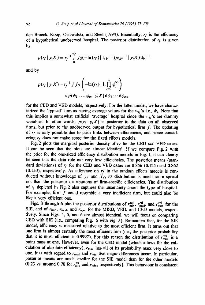
den Broeck, Keep, Osiewalski, and Steel (1994). Essentially, rf is the efficiency of a hypothetical unobserved hospital. The posterior distribution of rf is given by

OO

p(rl ly, X )= r;-~ f f~(-ln(r:)l 1,#-~)p(p - ' I y ,X)d#- ' 0

and by

P(rf l y'X) = rfl f fG (-ln(rf ) l l' f i ~Pf '

x p(4'~ . . . . . ~'m I y,X)d~b~'"" d~m,

for the CED and VED models, respectively. For the latter model, we have characterized the 'typical' firm as having average values for the wij's i.e., ~j. Note that this implies a somewhat artificial 'average' hospital since the wifs are dummy variables. In other words, p(rfly, X) is posterior to the data on all observed firms, but prior to the unobserved output for hypothetical firm f . The updating of rf is only possible due to prior links between efficiencies, and hence consid- ering rf does not make sense for the fixed effects models.

Fig. 2 plots the marginal posterior density of rf for the CED and VED cases. It can be seen that the plots are almost identical. If we compare Fig. 2 with the prior for the one-sided efficiency distribution models in Fig. 1, it can clearly be seen that the data rule out very low efficiencies. The posterior means (standard deviations) of r/ for the CED and VED cases are 0.856 (0.125) and 0.862 (0.120), respectively. As inference on O in the random effects models is conducted without knowledge of yf and Xf, its distribution is much more spread out than the posterior distributions of firm-specific efficiencies. The distribution of t) depicted in Fig. 2 also captures the uncertainty about the bpe of hospital. For example, firm f could resemble a very inefficient firm, but could also be like a very efficient one.

Figs. 3 through 6 plot the posterior distributions of r ~ , r ~ d, and rm~x for the SIE, and of rmin, treed, and rmax for the MIED, VED, and CED models, respectively. Since Figs. 4, 5, and 6 are almost identical, we will focus on comparing CED with SIE (i.e., comparing Fig. 6 with Fig. 3). Remember that, for the SIE model, efficiency is measured relative to the most efficient firm. It turns out that one firm is almost certainly the most efficient firm (i.e., the posterior probability that it is most efficient is 0.9997). For this reason the distribution of r ~ is a point mass at one. However, even for the CED model (which allows for the cal- culation of absolute efficiency), r ,m has all ot its probability mass very close to one. It is with regard to rmcd and rmi, that major differences occur. In particular, posterior means are much smaller tbr the SIE model than for the other models (0.23 vs. around 0.70 for t'r~lmi, and train, respectively). This behaviour is consistent


7 . 5 0

6 . 0 0

4.50

3.00

1.50

.......... V E D

C E D

( m = 4 ) " a v e r a g e

0.00 0 .005 .105 .205 .305 .405 .505 .605 .705 .805

// "] jt

/ /

, /

Fig. 2, Posteriors for r ( f ) (P: = 0.8).

. 9 0 5 . 995

2 1 . 0 0

16 .80

12 .60

8.40

4.20

0 . 0 0 -

0 . 0 0 5 . 1 0 5 . 6 0 5 . 2 0 5 . 3 0 5

j t i I

w l a 1 j

#

t i

. 405 . 505

io@int mass

.......... m i n e f f .

. . . . . m e d e f f .

. . . . . m a x e f f .

. 705 .805 . 9 0 5 .995

Fig. 3. Posteriors for efficiencies, SIE model,

with the important difference between the SIE and one-sided distribution models. The implied prior on r~ el (see Fig. 1) simply does not rule out very low relative efficiencies for many firms. From the fact that the posterior results for the MIED model (with r* =0.8) are quite close to those of the random effects models, we refer that it is not the fixed effects nature that induces the SIE model to behave so differently from the rest. Rather, it is the improper prior structure on the intercepts.

94 G. Koop et ai./Journal of Econometrics 76 (19~7) 77-105

2 1 . 0 0

1 6 . 8 0

1 2 . 6 0

8 . 4 0

4 . 2 0

.......... m i n

. . . . . m e d

. . . . . m a x

o.oo 0 . 0 0 5 . 1 0 5 . 2 0 5

e f f .

e f f .

e f f .

?

?

• 3 0 5 . 4 0 5 . 5 0 5 . 6 0 5 . 7 0 5

6 0 . 1 ' ~ :

! t I |

!

I t

, I ! t I

I t I |

I I I

I : ; \

. 8 0 5 . 9 0 5 . 9 9 5

Fig. 4. Posteriors for efficiencies, MIED model (r* = 0.8).

2 1 . 0 0

16 .80

1 2 . 6 0

8 . 4 0

4 . 2 0

.......... rain

. . . . . r e e d

. . . . . m a x

e f f . 58'51' 1

e f f . i i

e f f . . i l

F I ' : 1 I I -I I

• ' # I i : 1 ' I I ~ I , ! I ! ; I

! i . I I I j I ' 1

• ; I i 1 I

; I 'I,I . - p I~ I : ' i I t l • : ~ f~l : I I'1 I

" : i I ' d

• ' ", I | /I : ', t/ I

• ' , I t . ' , ~ s . . _ , J

0 . 0 0 0 . 0 0 5 . 1 0 5 . 2 0 5 . 3 0 5 . 4 0 5 . 5 0 5 . 6 0 5 . 7 0 5 . 8 0 5

Fig. 5. Postefiors~refficiencies, VED m ~ e l ( r * = 0 . 8 , m =4) .

. 905 . 9 9 5

If we replace the one-sided prior distribution (with r* =0.8) on the inefficiencies by the improper prior structure of the SIE model, we tend to substantially decrease the hospital efficiencies. Over~.ll, the average posterior mean efficiency is 0.47 for the SIE model and around 0.85 for the one-sided efficiency distribu-

G. Koop et al. IJour~iat of Econometrics 76 (1997) 77 105 95

21 .00

16.80

12.60

8 .40

4 .20

0 .00 0 . 0 0 5 . 1 0 5

.......... m i n e l f .

. . . . . r e e d e f f .

. . . . . m a x e f f .

6o41

..." " . .

.205 .305 .405 .505 .605 .705 .805

Fig. 6. Postefiors ~refficiencies, CED model(r* =0.8).

\ I 1 I

1

I!

I

I | l t l

l i t

e I J

.905 .995

tion models. However, the differences go beyond merely decreasing efficiency of each hospital; in many cases the ranking of efficiencies changes. The Spearman rank correlation between the n-vector of posterior means of hospital-specific efficiencies for the SIE and CED cases is only 0.43.

To illustrate the fact that the standard individual effects model considers relative, rather than absolute, measures of efficiency, we have eliminated the firm with the highest value of &~ (which was most efficient with probability 0.9997). Then we need to consider six candidates for most efficient firm in order to cap- turc a probability mass of at least 0.999, and the average posterior mean etii- ciency jumps to 0.55. Using the CED model on this reduced sample leads to an average posterior mean efficiency of 0.85, which hardly differs from that with the full sample. The results from the one-sided models are, in our subjective opinion, much more reasonable than those of the SIE model, both in terms of the efficiency measures (is it reasonable that, as the SIE model would have, there are many hospitals with efficiencies less than 30% of the most efficient firm?) and the frontier itself (fewer suggestions that regularity conditions are violated for the one-sided cases) Thus, we would advise against use of the SIE model. Therefore, in the rest of the discussion of our empirical results, we will primarily concentrate on the one-sided efficiency distribution models.

Even for the one-sided distribution models, the inference on firm-specific efficiencies suggests that cost-minimization is not achieved by many of the hospitals in our sample. Our analysis cannot tell us, however, whether this fact is due to managerial error, to some missing output (e.g., quality of care) or to a different objective function.

96 G Koop et al. I Journal of Econometrics 76 (1997) 77-105

Prior sensitivity analysis The one-sided individual effects models are based upon proper priors for effi-

ciencies. We believe that we have elicited quite reasonable priors, but it is always important to carry out a sensitivity analysis to see if the choice of prior hyperparameters (in our case r*) has an important effect on our results. This prior hyperparameter r* has the interpretation of the prior median efficiency for both the MIED and CED models. Let us compare these two models, as this enables us to isolate the effect of prior independence. For our previous discussions, we have set r*= 0.8, implying that we assign a prior probability of 0.5 to any hospital being less than 80 percent efficient.

Fig. 7 displays the average of posterior mean efficiencies over the 382 hospitals within the sample, say F, as a function of r*. The striking feature of these graphs is t ~ t F is virtually constant over the whole range of r* from 0.01 until 0.99 for the CED model. It seems the random effect nature of this model links the effi¢iencies sufficiently to ensure that the data dominate the prior information. In sharp contrast, the fixed effects MIED model does not lead to such robustness, as F varies substantially with r*. The independence assumption inhereat to this model, combined with the small value of T, implies that the data information on each individual efficiency is much weaker than in the CED case. If we take a value of r* in line with the data, say r* = 0.8, then both models lead to virtually the same inference on firm efficiencies, but if we deviate from ~uch a prior median efficiency, differences between the models grow. As r* becomes very small, the MIED model will have marginal priors on the efficiencies that are still proper, but will start to look like the marginal priors on relative efficiencies for the SIE model. As both models are fixed effects models and their only difference lies in the fbrm of the marginal prio~, we find, indeed, that results for the MIED model with r* = 0.01 are relatively close to the SIE model.

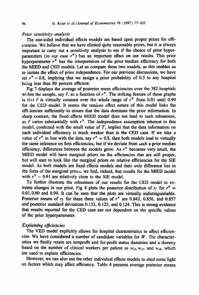
To further illustrate the robustness of our results for the CED model to ex- treme changes in our prior, Fig. 8 plots the posterior distribution of rf for r* = 0.01,0.80 and 0.99. It can be seen that the plots are virtually indistinguishable. Posterior means of rf for these three values of r* are 0.843, 0.856, and 0.857 and posterior standard deviations 0.133, 0.125, and 0.124. This is strong evidence that results reported for the CED case are not dependent on the specific values of the prior hyperparameter.

Explaining efficiencies The VED model explicitly allows for hospital characteristics to affect efficien-

cies. We have considered a number of candidate variables for W. The characteristics we finally retain are nonprofit and for-profit status dummies and a dummy based on the number of clinical workers per patient as w~2, w~3, and wi4, which are used to explain efficiencies.

However, we can also use the other individual effects models to shed some light on fhctors which may affect efficiency. Table 4 presents average posterior means

1.00

0 . 9 0

0.80

0.70

0 . 6 0

0 . 5 0 0.01

................ M I E D

. . . . . . . . C E D


. . . - " "

, . . . . . " , . . , "

. . . . . . . ' " "

7 . 5 0

0.21 0 .40 0 . 6 0 0.79

Fig. 7. Average posterior mean efficiency as a function of r*.

0.99

6 . 0 0

4 . 5 0

3 . 0 0

1 .50

0.00 0 .005 .105 .205 .305

............. r-X- = 0 . 0 1

. . . . . . . . r - X - = 0 . 8

r - X - = 0 . 9 9

. . . .

• 4 0 5 . 505 .605 .705 . 8 0 5 .905 .995

Fig. 8. Sensitivity of p(r(f)ly, X), CED model.

and standard deviations of individual efficiencies for for-profit, nonprofit, and government-run hospitals. Once again, the one-sided efficiency cases yield very similar results for r* = 0.8. However, results for the SIE model are quite different. For the random effects models a clear pattern emerges: for-profit hospitals are less efficient than nonprofit or government-run hospitals.

98 G. Keep et al./Journal of Econometrics 76 (1997) 77-105

Table 4 Averages of posterior means of efficiencies for hospital subgroups (averages of posterior standard deviations in parentheses)

Nonprofit For-profit Govt.-run All

SIE 0.456 0.485 0.502 0.467 (0.028) (0.029) (0.029) (0.028)

MIED 0.853 0.819 0.821 0.843 (0.026) (0.027) (0.028) (0.026)

VED 0.866 0.793 0.871 0.855 (0.026) (0.027) (0.026) (0.026)

CED 0.861 0.796 0.870 0.851 (0.026) (0.027) (0.026) (0.026)

Table 5 Posterior means and standard deviations of 7

71 72 Y3 ~4

Mean 2.05 -0.02 -0.50 -0.25 Std. dev 0.16 0.16 0.19 0.11

The varying efficiency distribution model allows us to investigate directly the effect of the w,'s on efficiency. Posterior means and standard deviations for the elements of)' are given in Table 5. The posterior means of )' given in Table 5 are consistent with government-run hospitals being most efficient followed by nonprofit and for-profit hospitals. An approximate Bayesian Highest Posterior Density interval test (see Zell!vler, 1971, pp. 298-302) favours the VED model. Remem- ber that the CED model is equal to the VED model with ~2 = " " = )'m ~ 0. If the posterior for the i~'j's ( j = 2 . . . . ,m) is approximately Normal, then the distribution of the inner product of the standardized )'y's is approximately Z~-i. For our data, this quantity, evaluated at zero, is 17.50. Since m = 4, this indicates that the VED model provides explanatory power beyond the CED model.

The strongest findiing is that for-profit status tends to decrease hospital efficiency. In addition, the posterior mean of )'4, the coefficient on the dummy for high worker to patient ratios, indicates that having a greater number of workers tends to decrease efficiency as well. The posterior means of )'3 and )'4 are both more than two standard deviations from zero. We find the result that for-profit hospitals tend to be less efficient than other hospitals counter-intuitive. One possible explanation is that for-profit hospitals tend to compete by offering higher quality service. Since it is hard to directly observe quality, low efficiency might actually be capturing higher quality. However, one way in which hospitals can offer higher quality is by providing more clinical personnel. The fact that 73 is

G. Koop et aL /Journal of Econometrics 76 (1997) 77-105 99

7.50

6.00

4.50

3 .00

1.50

0 .00 0 . 0 0 5 . 105

.............. non-prof i t

. . . . . . . . for -prof i t /

government /

L' " J ~ • 2 0 5 .305 .405 .505 .605 .705 .805 .905 .995

Fig. 9. p(r(f)[y,X) for hospital types, VED model (r* = 0.8,m = 4).

still significant when w4 is added indicates that this latter mechanism for improv- ing quality does not suffice to explain the failure of for-profit hospitals to achieve high efficiency.

In Koop, Osiewalski, and Steel (1994a), a relative predictive measure of lack of fit is developed, a detailed justification of which is given therein. If we let ~ft = UJ'q-Of t , then we advocate using EO:t~Iy, X) = E(a2+ 2#21Y, X) as a measure of fit for the CED model. For the VED model, exp(-w~,) is anal- ogous to /~, so we use E(tr2 + 2exp(-2~'y) ly , X,W), where ~ is the average of the w~'s, which we use tbr wf corresponding to the average firm. The measure of fit is 0.061 for the CED model and 0.056 for the VED model. In other words, in terms of our measure of fit, the VED model does better. We cam~ot construct a comparable measure for the other models. However, note the posterior mean of a 2 is 0.0034 for the SIE model, 0.0042 for fl,e MIED, and 0.0043 for both random effects models. The fact that the prior of the SIE model strongly favours low efficiencies implies that measurement error is smaller for this latter model, as much more of the total error is allocated to inefficiency.

Fig. 9 plots the posterior density of rf for nonprofit, for-profit, and government- run hospitals based on the VED model. Corresponding means (standard deviations) are 0.871 (0.114), 0.806 (0.161), and 0.872 (0.114) for nonprofit, fo,- profit, and government-run hospitals, respectively. This merely reinforces our previous conclusions, viz. that for-profit hospitals tend to be less efficient than other hospitals.


5. Conclusion

In this paper we have described and analyzed Bayesian models for inference on finn-specific efficiencies. We show how, by using different prior sUactures, we can derive Bayesian analogues to the classical fixed and random individual effects models. The fixed effects models are characterized by the absence of links between individual effects, and thus do not require a hierarchical prior structure. Within this class, we define the standard individual effects (SIE) model, which puts an improper uniform prior on the finn-specific intercepts and measures relative efficieneies in terms of differences between the intercepts, and the marginally independent efficiency distribution (MIED) model, where independent proper one-sided priors are used for individual effects, and efficiencies are thus defined in absolute terms. Bayesian random effects models do link individual effects through the hierarchical structure of the prior, parameterizing the n effects in terms of a small number m <~n of additional parameters. The common efficiency distribution (CED) model takes m = 1 and assigns a common exponential prior distribution to inefficiencies; the varying efficiency distribution (VED) model allows the mean of the exponential prior to vary according to m - 1 hospital characteristics.

The seemingly innocuo~,s fiat prior on individual intercepts associated with the SlE model enables us to reinterpret many classical results in a Bayesian context. However, adoption of this model necessarily implies a strong prior belief in low firm efficiencies, which is very different from those commonly held. Fur- thermore, the fixed effects nature of this model makes it diffic~dt for the data to correct this prior information when T is small. For this reason, we would advocate using the one-sided individual effects models for inference on efficiencies in a stochastic frontier context. Whereas the MIED model allows us to capture our prior beliefs through any proper distribution, its fixed effects structure still implies a large sensitivity to the choice of the particular prior when T is not large. Furthermore, the lack of links between individual effects inherent to fixed effects models make prediction of these effects for unobserved firms a useless exercise.

We apply our methods to a panel of U.S. hospitals and obtain reasonable results for both random effects models, which display an impressive robustness with respect to large changes in our prior hyperparameter.

Appendix

SIE model

The SIE model can be analyzed using Monte Carlo integration. The marginal posterior for the parameters of the cost frontier, ~, is the k-variate Normal

G. Koop et al./ Journal of Econometrics 76 (1997) 77-105 101

distribution with n

E(flly, X ) = fl = S -~ ~" (X~ - ~rYc~)'(y~ - :P,~r), i=1

where

1 I 1 I Xi = -~Xi IT, fii = -~ITYi '

(A.1)

n

s i - (x~ - z r ~ ) ' ( x ~ - ~ r ~ ) , S = ~ s , . i=1

Eq. (A.1) is the so-called 'within estimator' from the panel data literature. The covariance matrix for the marginal posterior for fl is given by

V(fl]y,X) = b2S - i , (A.2)

where

~2 = 1 n ^ I (Yi - &~*r - X i f l ) ( Y i - &i*r -Xif3). n ( T - 1 ) - k i=l

The marginal posterior of • is the n-variate Normal distribution with means

E(otily, X ) = & i = ~i-.~[fl , i = 1, . . . . n, (A.3)

and covariances

cov(~i,~jly, X ) = (r2 ( 6 ( T J ) + £ , S - ' £ j ) , i , j = l , . . . ,n , (A.4)

where 6( i , j ) = 1 if i = j and 0 otherwise. Since the ~t~.'s are Normally distributed, it follows that the marginal posterior

of r/(j) is the ( n - l)-variate Normal distribution with means

E(~llJ)ly, X ) = &~ - &j,

and covariances

c o v ( , l J ~ . . l ~ J ~ l y . X ) = ~ ~ ( £ ~ - ~ j ) ' s - ~ ( ~ h - ~ j ) + - , .

• t J) is ej- - e j . for i, h = 1, . . . , n, i ¢ j , h # j , where '1i

MIED model

The conditional distributions used in the Gibbs sampler have simple forms. In particular, conditional on u and 2 -I = (2~-I .. . 2~ -l )', the posterior density of the frontier parameters and precision, e - 2 has the usual Normal-Gamma form:

p(oto,[J, tr-2lY, X,u,2 -I ) = p(a-21y, X,u)p(oto, flly, X,u ,a-2) , (A.5)

102

where

p(tr-2ly, X,u)=fG(tr-2 I

and

G Koop et al./Journal qf Econometrics 76 (1997) 77-105

n T - k - 1 2

(A.6)

-'). (A.7)

where

and

f i , = ~1 ~ Yit, U = - Ui, l i t i=l t=l n i=l

T ,¢,= __! Ex,,. RT i=l ~=!

The conditional posterior for the inefficiencies takes the form:

p(uly, X, O~o,/3, ~-2, 2-1 )

cxf~v(ul.~-(tn:,~,(~fl°) -tT2.;-' ~-In) xI+(u),

p(uly, X, O~o,/3, ~-2, 2-1 )

T .v

(i) ?= , £= n

(z'~ / '

z , /

and l+(u) is the indicator function for R~.. In other words, the ui's are indepen- dently Normally distributed, but truncated to the positive orthant. The conditional

(A.8)

Here,

In the previous equations, s~(.la, b) denotes the density function of the Gamma distribution with mean a/b and variance a/b:, y = (yl... Y,,)', an nT x 1 vector, X = ( X ( . " • .X,~), an n T x k matrix, and

~, - l ( nr(?* - ~) ) X'X ~,X'y - X'(l. ® tr)U "


posterior for 2 -I becomes

n

P(A-lly, X,u,~o, fl, ~-2) = P ( 2 - ~ I u) = 1-I J~(A/-ll2,u~ - I n ( r * ) ) . i=l

(A.9)

A Gibbs sampler can be set up in terms of Eqs. (A.5), (A.8), and (A.9). Random sampling from all these densities is standard. Note that, despite the high dimensionality of the problem (2n + k + 2 = 803 in our problem), three steps suffice for each Gibbs draw. It is worth stressing that this specification assumes a separate efficiency distribution for each firm. Thus, conditionally upon the parameters describing the frontier, the u : s are posterior independent and are only updated by the T observations for firm i, similarly as the ~ ' s in the SIE model.

VED model

The conditional posterior for the frontier parameters is identical to that given previously in Eqs. (A.5), (A.6), and (A.7). The conditional posterior for the inefficiencies takes the form:

p(uly, X, W, ~0, fl, tr -2, ?) _ _ 0 -2

x l+(u), (A.10)

where ~ = (exp(w~,)...exp(w'n~,))'. In other words, the u;'s are again indepen- dently Normally distributed, truncated to the positive orthant. The conditional distribution of any of the ~bj,'s (~bh = exp(~,h), h = l , . . . ,m) depends only on u and q~(-h) = (61, . . . . t/~h-I, q~h+l, . . . . ¢km)' and is given by

P(~bhlW'u'dp(-h))= fG (~bh[ah + ~ wih'ffh + ~ Wihu~ l-[ ~bT'J) i=1 yeh (A.11)

With the Gibbs sampler we now have to deal with numerical integration in only n + k + m + 2 dimensions (423 in our empirical application).

CED model

The Gibbs sampler can be implemented by cyclical drawings from (A.5) and (A.8) , where 2 -~ = #-zt , , , and from the full conditional for #- l which is

p(#-l]y,X,u,~,fl, 0- -2) = p(#-Ilu ) = f~(#-~ I(n + 1), n a - In(r*)). (A.12)


References

Aigner, D., C. Lovell, and P. Schmidt, 1977, Formulation and estimation of stochastic frontier production function models, Journal of Econometrics 6, 21-37.

Allenby, G., R. McCuUoch, and P. Rossi, 1995, Hierarchical probit models with applications to target couponing, in: R. Kass and N. Singpurwalla, eds., Bayesian case studies, forthcoming.

Box, G.E.P. and G.C. Tiao, 1973, Bayesian inference in statistical analysis (Addison-Wesley, Reading, MA).

Breyer, F., 1987, The specification of a hospital cost function: A comment on the recent literature, Journal of Health Economies 6, 147-157.

Broeck J. van den, G. Keep, J. Osiewalski, and M.F.J. Steel, 1994, Stochastic frontier models: A Bayesian perspective, Journal of Econometrics 61,273-303.

Cowing, T., ~. Holtman, and S. Powers, 1983, Hospital cost analysis: A survey and evaluation of recent studies, Advances in Health Economics and Health Services Research 4, 257-303.

Dor, A., 1994, Non-minimum cost functions and the stochastic frontier: On applications to health care providers, Journal of Health Economics 13, 329-334.

Eakin, B. and T. Kniesner, 1988, Estimating a non-minimum cost function for hospitals, Southern Economic Journal 54, 583-597.

Engle, R.F., D.F. Hendry, and J.F. Richard, 1983, Exogeneity, Econometrica 51,277-304. Farrell, M., 1957, The measurement of productive efficiency, Journal of the Royal Statistical Society

A 120, 253-281. Gelfand, A. and AILM. Smith, 1990, Sampling-based approaches to calculating marginal densities,

Journal of the American Statistical Association 85, 398-409. Grannemann, T., R. Brown, and M. Pauly, 1986, Estimating hospital costs: A multiple-output analysis,

Journal of Health Economics 5, 107-127. Keep, G., 1994, Recent progress in applied Bayesian econometrics, Journal of Economic Surveys 8,

1-34. Keep, G., J. Osiewalski, and M. Steel, 1994a, Bayesian efficiency analysis with a flexible form: The

AIM cost function, Journal of Business and Economic Statistics 12, 93-106. Keep, G., J. Osiewalski, and M. Steel, 1994b, Hospital efficiency analysis with individual effects: A

Bayesian approach, Center for Economic Research discussion paper no. 9447 (Tilburg University, Tilburg).

Keep, G., MF.J. Steel, and J. Osiewalski, 1995, Posterior analysis of stochastic frontier models using Gibbs sampling, Computational Statistics 10, 353-373.

Kopp, R. and W.E. Diewert, 1982, The decomposition of frontier cost fu,ction deviations into measures of technical and allocative inefficiency, Journal of Econometrics 19, 319-332.

Lindle~, D. and A.F.M. Smith, 1972, Bayes estimates for the linear model, Journal of the Royal Statistical Society B 34, 1-41.

McCulloch, R. and P.E. Rossi, 1994, An exact likelihood analysis of the mu!tinomial probit model, Journal of Econometrics 64, 207-240.

Meeusen, W. and J. van den Broeek, 1977, Efficiency estimation from Cobb-Douglas production functions with composed error, International Economic Review 8, 435-444.

Osiewalski, J. and M. Steel, 1996, A Bayesian analysis of exogeneity in models pooling time-series and cross-section data, Journal of Statistical Planning and Inference 50, 187-206.

Pitt, M. and L.-F. Lee, 1981, The measurement and sources of technical inefficiency in the Indonesian weaving industry, Journal of Development Economics 9, 43-64.

Schmidt, P. and R. Sickles, 1984, Production frontiers and panel dat~. Journal of Business and Economic Statistics 2, 367--374.

Simar, L., 1992, Estimating efficieneies from frontier models with panel data: A comparison of parametric, non-parametric and semi-parametric methods with bootstrapping, Journal of Productivity Analysis 3, 171-203.


Skinner, J., 1994, What do stochastic frontier cost functions tell us about efficiency?, Journal of Health Economics 13, 323-328.

Tierney, L., 1991, Exploring posterior distributions using Markov chains, in: E.M. Keramidas and S.M. Kaufman, eds., Computing science and statistics: Proceedings of the 23rd symposium on the interface (Interface Foundation of North America, Fairfax, VA).

Vita, M., 1990, Exploring hospital production relationships with flexible functional forms, Journal of Health Economies 9, !-21.

Vitaliano, D. and M. Toren, 1994a, Cost and efficiency in nursing homes: A stochastic frontier approach, Journal of Health Economies 13, 281-300.

Vitaliann, D. and M. Torch, 1994b, Froh'ier analysis: A reply to Skinner, Dor and Newhouse, Journal of Health Economies 13, 341-343.

Zellner, A., 1971, An introduction to Bayesian inference in econometrics (Wiley, New York, NY). Zuckerman, S., J. Hadley, and L. lezzoni, 1994, Measuring hospital efficiency with ~ontier cost

functions, Journal of Health Economics 13, 255-280.

Koop, Osiewalski and Steel - NYU Stern School of Business

Documents

Transcript of Koop, Osiewalski and Steel - NYU Stern School of Business