CS240A: Databases and Knowledge Bases Temporal Applications and SQL:1999
Knowledge Bases and DatabasesPart 1: First-Order Queries
Diego Calvanese
Faculty of Computer ScienceMaster of Science in Computer Science
A.Y. 2008/2009
unibz.itunibz.it
Overview of Part 1: First-order queries
1 First-order logic1 Syntax of first-order logic2 Semantics of first-order logic3 First-order logic queries
2 First-order query evaluation1 Query evaluation problem2 Complexity of query evaluation
3 Conjunctive queries1 Evaluation of conjunctive queries2 Containment of conjunctive queries [Optional]3 Unions of conjunctive queries
D. Calvanese Part 1: First-Order Queries KBDB – 2008/2009 (1/65)
unibz.itunibz.it
Syntax of first-order logic Semantics of first-order logic First-order logic queries
Chap. 1: First-Order Logic
Chapter I
First-Order Logic
D. Calvanese Part 1: First-Order Queries KBDB – 2008/2009 (2/65)
unibz.itunibz.it
Syntax of first-order logic Semantics of first-order logic First-order logic queries
Chap. 1: First-Order Logic
Outline
1 Syntax of first-order logic
2 Semantics of first-order logic
3 First-order logic queries
D. Calvanese Part 1: First-Order Queries KBDB – 2008/2009 (3/65)

unibz.itunibz.it
Syntax of first-order logic Semantics of first-order logic First-order logic queries
Chap. 1: First-Order Logic
Outline
1 Syntax of first-order logic
2 Semantics of first-order logic
3 First-order logic queries
D. Calvanese Part 1: First-Order Queries KBDB – 2008/2009 (4/65)
unibz.itunibz.it
Syntax of first-order logic Semantics of first-order logic First-order logic queries
Chap. 1: First-Order Logic
First-order logic
First-order logic (FOL) is the logic to speak about objects, whichare the domain of discourse or universe.
FOL is concerned about properties of these objects and relationsover objects (resp., unary and n-ary predicates).
FOL also has functions including constants that denote objects.
D. Calvanese Part 1: First-Order Queries KBDB – 2008/2009 (5/65)
unibz.itunibz.it
Syntax of first-order logic Semantics of first-order logic First-order logic queries
Chap. 1: First-Order Logic
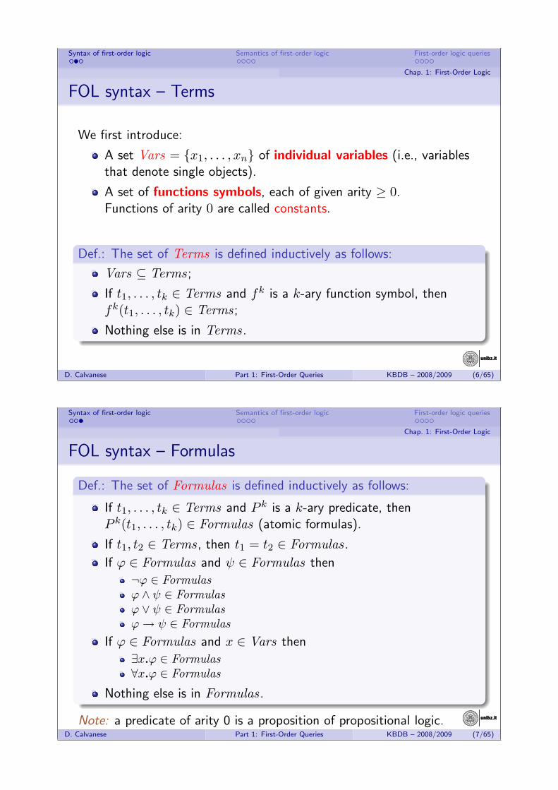
FOL syntax – Terms
We first introduce:
A set Vars = {x1, . . . , xn} of individual variables (i.e., variablesthat denote single objects).
A set of functions symbols, each of given arity ≥ 0.Functions of arity 0 are called constants.
Def.: The set of Terms is defined inductively as follows:
Vars ⊆ Terms;
If t1, . . . , tk ∈ Terms and fk is a k-ary function symbol, thenfk(t1, . . . , tk) ∈ Terms;
Nothing else is in Terms.
D. Calvanese Part 1: First-Order Queries KBDB – 2008/2009 (6/65)
unibz.itunibz.it
Syntax of first-order logic Semantics of first-order logic First-order logic queries
Chap. 1: First-Order Logic
FOL syntax – Formulas
Def.: The set of Formulas is defined inductively as follows:
If t1, . . . , tk ∈ Terms and P k is a k-ary predicate, thenP k(t1, . . . , tk) ∈ Formulas (atomic formulas).
If t1, t2 ∈ Terms, then t1 = t2 ∈ Formulas.
If ϕ ∈ Formulas and ψ ∈ Formulas then
¬ϕ ∈ Formulasϕ ∧ ψ ∈ Formulasϕ ∨ ψ ∈ Formulasϕ→ ψ ∈ Formulas
If ϕ ∈ Formulas and x ∈ Vars then
∃x.ϕ ∈ Formulas∀x.ϕ ∈ Formulas
Nothing else is in Formulas.
Note: a predicate of arity 0 is a proposition of propositional logic.D. Calvanese Part 1: First-Order Queries KBDB – 2008/2009 (7/65)
unibz.itunibz.it
Syntax of first-order logic Semantics of first-order logic First-order logic queries
Chap. 1: First-Order Logic
Outline
1 Syntax of first-order logic
2 Semantics of first-order logic
3 First-order logic queries
D. Calvanese Part 1: First-Order Queries KBDB – 2008/2009 (8/65)
unibz.itunibz.it
Syntax of first-order logic Semantics of first-order logic First-order logic queries
Chap. 1: First-Order Logic
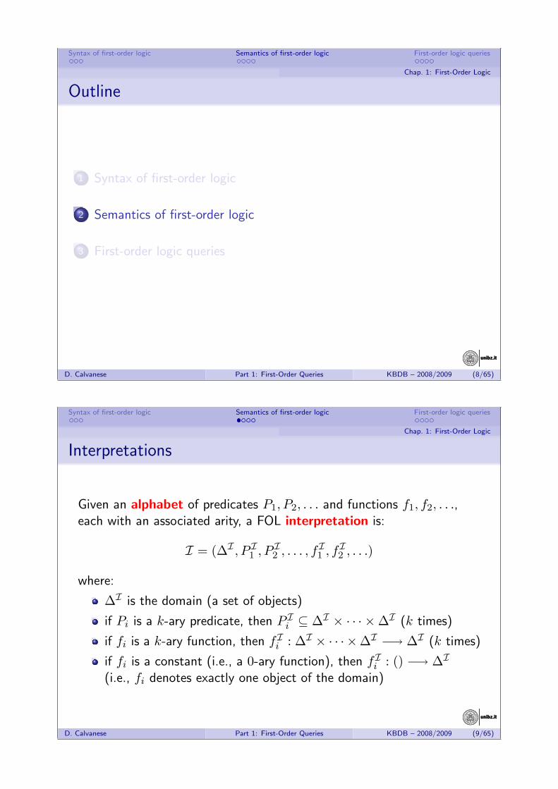
Interpretations
Given an alphabet of predicates P1, P2, . . . and functions f1, f2, . . .,each with an associated arity, a FOL interpretation is:
I = (∆I , P I1 , PI2 , . . . , f
I1 , f
I2 , . . .)
where:
∆I is the domain (a set of objects)
if Pi is a k-ary predicate, then P Ii ⊆ ∆I × · · · ×∆I (k times)
if fi is a k-ary function, then fIi : ∆I × · · · ×∆I −→ ∆I (k times)
if fi is a constant (i.e., a 0-ary function), then fIi : () −→ ∆I
(i.e., fi denotes exactly one object of the domain)
D. Calvanese Part 1: First-Order Queries KBDB – 2008/2009 (9/65)
unibz.itunibz.it
Syntax of first-order logic Semantics of first-order logic First-order logic queries
Chap. 1: First-Order Logic
Assignment
Let Vars be a set of (individual) variables.
Def.: Given an interpretation I, an assignment is a function
α : Vars −→ ∆I
that assigns to each variable x ∈ Vars an object α(x) ∈ ∆I .
It is convenient to extend the notion of assignment to terms. We can doso by defining a function α̂ : Terms −→ ∆I inductively as follows:
α̂(x) = α(x), if x ∈ Varsα̂(f(t1, . . . , tk)) = fI(α̂(t1), . . . , α̂(tk))
Note: for constants α̂(c) = cI .
D. Calvanese Part 1: First-Order Queries KBDB – 2008/2009 (10/65)
unibz.itunibz.it
Syntax of first-order logic Semantics of first-order logic First-order logic queries
Chap. 1: First-Order Logic
Truth in an interpretation wrt an assignment
We define when a FOL formula ϕ is true in an interpretation I wrt anassignment α, written I, α |= ϕ:
I, α |= P (t1, . . . , tk) if (α̂(t1), . . . , α̂(tk)) ∈ P II, α |= t1 = t2 if α̂(t1) = α̂(t2)I, α |= ¬ϕ if I, α 6|= ϕI, α |= ϕ ∧ ψ if I, α |= ϕ and I, α |= ψI, α |= ϕ ∨ ψ if I, α |= ϕ or I, α |= ψI, α |= ϕ→ ψ if I, α |= ϕ implies I, α |= ψI, α |= ∃x.ϕ if for some a ∈ ∆I we have I, α[x 7→ a] |= ϕI, α |= ∀x.ϕ if for every a ∈ ∆I we have I, α[x 7→ a] |= ϕ
Here, α[x 7→ a] stands for the new assignment obtained from α asfollows:
α[x 7→ a](x) = aα[x 7→ a](y) = α(y) for y 6= x
D. Calvanese Part 1: First-Order Queries KBDB – 2008/2009 (11/65)
unibz.itunibz.it
Syntax of first-order logic Semantics of first-order logic First-order logic queries
Chap. 1: First-Order Logic
Open vs. closed formulas
Definitions
A variable x in a formula ϕ is free if x does not occur in the scopeof any quantifier, otherwise it is bound.
An open formula is a formula that has some free variable.
A closed formula, also called sentence, is a formula that has nofree variables.
For closed formulas (but not for open formulas) we can define what itmeans to be true in an interpretation, written I |= ϕ, withoutmentioning the assignment, since the assignment α does not play anyrole in verifying I, α |= ϕ.
Instead, open formulas are strongly related to queries — cf. relationaldatabases.
D. Calvanese Part 1: First-Order Queries KBDB – 2008/2009 (12/65)
unibz.itunibz.it
Syntax of first-order logic Semantics of first-order logic First-order logic queries
Chap. 1: First-Order Logic
Outline
1 Syntax of first-order logic
2 Semantics of first-order logic
3 First-order logic queries
D. Calvanese Part 1: First-Order Queries KBDB – 2008/2009 (13/65)
unibz.itunibz.it
Syntax of first-order logic Semantics of first-order logic First-order logic queries
Chap. 1: First-Order Logic
FOL queries
Def.: A FOL query is an (open) FOL formula.
When ϕ is a FOL query with free variables (x1, . . . , xk), then wesometimes write it as ϕ(x1, . . . , xk), and say that ϕ has arity k.
Given an interpretation I, we are interested in those assignments thatmap the variables x1, . . . , xk (and only those). We write an assignmentα s.t. α(xi) = ai, for i = 1, . . . , k, as 〈a1, . . . , ak〉.
Def.: Given an interpretation I, the answer to a query ϕ(x1, . . . , xk) is
ϕ(x1, . . . , xk)I = {(a1, . . . , ak) | I, 〈a1, . . . , ak〉 |= ϕ(x1, . . . , xk)}
Note: We will also use the notation ϕI , which keeps the free variablesimplicit, and ϕ(I) making apparent that ϕ becomes a functions frominterpretations to set of tuples.
D. Calvanese Part 1: First-Order Queries KBDB – 2008/2009 (14/65)
unibz.itunibz.it
Syntax of first-order logic Semantics of first-order logic First-order logic queries
Chap. 1: First-Order Logic
FOL boolean queries
Def.: A FOL boolean query is a FOL query without free variables.
Hence, the answer to a boolean query ϕ() is defined as follows:
ϕ()I = {() | I, 〈〉 |= ϕ()}
Such an answer is
(), if I |= ϕ
∅, if I 6|= ϕ.
As an obvious convention we read () as “true” and ∅ as “false”.
D. Calvanese Part 1: First-Order Queries KBDB – 2008/2009 (15/65)
unibz.itunibz.it
Syntax of first-order logic Semantics of first-order logic First-order logic queries
Chap. 1: First-Order Logic
FOL formulas: logical tasks
Definitions
Validity: ϕ is valid iff for all I and α we have that I, α |= ϕ.
Satisfiability: ϕ is satisfiable iff there exists an I and α such thatI, α |= ϕ, and unsatisfiable otherwise.
Logical implication: ϕ logically implies ψ, written ϕ |= ψ iff for allI and α, if I, α |= ϕ then I, α |= ψ.
Logical equivalence: ϕ is logically equivalent to ψ, iff for all I andα, we have that I, α |= ϕ iff I, α |= ψ (i.e., ϕ |= ψ and ψ |= ϕ).
D. Calvanese Part 1: First-Order Queries KBDB – 2008/2009 (16/65)
unibz.itunibz.it
Syntax of first-order logic Semantics of first-order logic First-order logic queries
Chap. 1: First-Order Logic
FOL queries – Logical tasks
Validity: if ϕ is valid, then ϕI = ∆I × · · · ×∆I for all I, i.e., thequery always returns all the tuples of I.
Satisfiability: if ϕ is satisfiable, then ϕI 6= ∅ for some I, i.e., thequery returns at least one tuple.
Logical implication: if ϕ logically implies ψ, then ϕI ⊆ ψI for allI, written ϕ ⊆ ψ, i.e., the answer to ϕ is contained in that of ψ inevery interpretation. This is called query containment.
Logical equivalence: if ϕ is logically equivalent to ψ, then ϕI = ψI
for all I, written ϕ ≡ ψ, i.e., the answer to the two queries is thesame in every interpretation. This is called query equivalence andcorresponds to query containment in both directions.
Note: These definitions can be extended to the case where we haveaxioms, i.e., constraints on the admissible interpretations.
D. Calvanese Part 1: First-Order Queries KBDB – 2008/2009 (17/65)
unibz.itunibz.it
Query evaluation problem Complexity of query evaluation
Chap. 2: First-Order Query Evaluation
Chapter II
First-Order Query Evaluation
D. Calvanese Part 1: First-Order Queries KBDB – 2008/2009 (18/65)
unibz.itunibz.it
Query evaluation problem Complexity of query evaluation
Chap. 2: First-Order Query Evaluation
Outline
4 Query evaluation problem
5 Complexity of query evaluation
D. Calvanese Part 1: First-Order Queries KBDB – 2008/2009 (19/65)
unibz.itunibz.it
Query evaluation problem Complexity of query evaluation
Chap. 2: First-Order Query Evaluation
Outline
4 Query evaluation problem
5 Complexity of query evaluation
D. Calvanese Part 1: First-Order Queries KBDB – 2008/2009 (20/65)
unibz.itunibz.it
Query evaluation problem Complexity of query evaluation
Chap. 2: First-Order Query Evaluation
Query evaluation
Let us consider:
a finite alphabet, i.e., we have a finite number of predicates andfunctions, and
a finite interpretation I, i.e., an interpretation (over the finitealphabet) for which ∆I is finite.
Then we can consider query evaluation as an algorithmic problem, andstudy its computational properties.
Note: To study the computational complexity of the problem, weneed to define a corresponding decision problem.
D. Calvanese Part 1: First-Order Queries KBDB – 2008/2009 (21/65)
unibz.itunibz.it
Query evaluation problem Complexity of query evaluation
Chap. 2: First-Order Query Evaluation
Query evaluation problem
Definitions
Query answering problem: given a finite interpretation I and aFOL query ϕ(x1, . . . , xk), compute
ϕI = {(a1, . . . , ak) | I, 〈a1, . . . , ak〉 |= ϕ(x1, . . . , xk)}
Recognition problem (for query answering): given a finiteinterpretation I, a FOL query ϕ(x1, . . . , xk), and a tuple(a1, . . . , ak), with ai ∈ ∆I , check whether (a1, . . . , ak) ∈ ϕI , i.e.,whether
I, 〈a1, . . . , ak〉 |= ϕ(x1, . . . , xk)
Note: The recognition problem for query answering is the decisionproblem corresponding to the query answering problem.
D. Calvanese Part 1: First-Order Queries KBDB – 2008/2009 (22/65)
unibz.itunibz.it
Query evaluation problem Complexity of query evaluation
Chap. 2: First-Order Query Evaluation
Query evaluation algorithm
We define now an algorithm that computes the function Truth(I, α, ϕ)in such a way that Truth(I, α, ϕ) = true iff I, α |= ϕ.
We make use of an auxiliary function TermEval(I, α, t) that, given aninterpretation I and an assignment α, evaluates a term t returning anobject o ∈ ∆I :
∆I TermEval(I,α,t) {if (t is x ∈ Vars)
return α(x);if (t is f(t 1, . . . , t k))
return fI(TermEval(I,α,t 1),...,TermEval(I,α,t k));}
Then, Truth(I, α, ϕ) can be defined by structural recursion on ϕ.
D. Calvanese Part 1: First-Order Queries KBDB – 2008/2009 (23/65)
unibz.itunibz.it
Query evaluation problem Complexity of query evaluation
Chap. 2: First-Order Query Evaluation
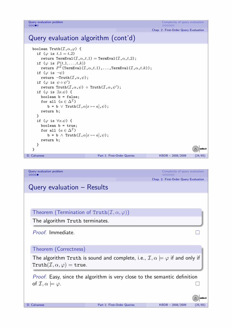
Query evaluation algorithm (cont’d)
boolean Truth(I,α,ϕ) {
if (ϕ is t 1 = t 2)return TermEval(I,α,t 1) = TermEval(I,α,t 2);
if (ϕ is P (t 1, . . . , t k))return PI(TermEval(I,α,t 1),...,TermEval(I,α,t k));
if (ϕ is ¬ψ)return ¬Truth(I,α,ψ);
if (ϕ is ψ ◦ ψ′)return Truth(I,α,ψ) ◦ Truth(I,α,ψ′);
if (ϕ is ∃x.ψ) {
boolean b = false;
for all (a ∈ ∆I)b = b ∨ Truth(I,α[x 7→ a],ψ);
return b;
}
if (ϕ is ∀x.ψ) {
boolean b = true;
for all (a ∈ ∆I)b = b ∧ Truth(I,α[x 7→ a],ψ);
return b;
}
}
D. Calvanese Part 1: First-Order Queries KBDB – 2008/2009 (24/65)
unibz.itunibz.it
Query evaluation problem Complexity of query evaluation
Chap. 2: First-Order Query Evaluation
Query evaluation – Results
Theorem (Termination of Truth(I, α, ϕ))
The algorithm Truth terminates.
Proof. Immediate.
Theorem (Correctness)
The algorithm Truth is sound and complete, i.e., I, α |= ϕ if and only ifTruth(I, α, ϕ) = true.
Proof. Easy, since the algorithm is very close to the semantic definitionof I, α |= ϕ.
D. Calvanese Part 1: First-Order Queries KBDB – 2008/2009 (25/65)
unibz.itunibz.it
Query evaluation problem Complexity of query evaluation
Chap. 2: First-Order Query Evaluation
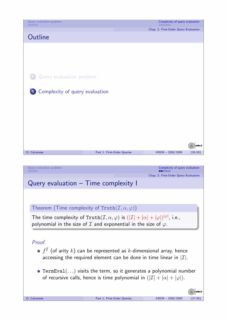
Outline
4 Query evaluation problem
5 Complexity of query evaluation
D. Calvanese Part 1: First-Order Queries KBDB – 2008/2009 (26/65)
unibz.itunibz.it
Query evaluation problem Complexity of query evaluation
Chap. 2: First-Order Query Evaluation
Query evaluation – Time complexity I
Theorem (Time complexity of Truth(I, α, ϕ))
The time complexity of Truth(I, α, ϕ) is (|I|+ |α|+ |ϕ|)|ϕ|, i.e.,polynomial in the size of I and exponential in the size of ϕ.
Proof.
fI (of arity k) can be represented as k-dimensional array, henceaccessing the required element can be done in time linear in |I|.
TermEval(. . .) visits the term, so it generates a polynomial numberof recursive calls, hence is time polynomial in (|I|+ |α|+ |ϕ|).
D. Calvanese Part 1: First-Order Queries KBDB – 2008/2009 (27/65)
unibz.itunibz.it
Query evaluation problem Complexity of query evaluation
Chap. 2: First-Order Query Evaluation
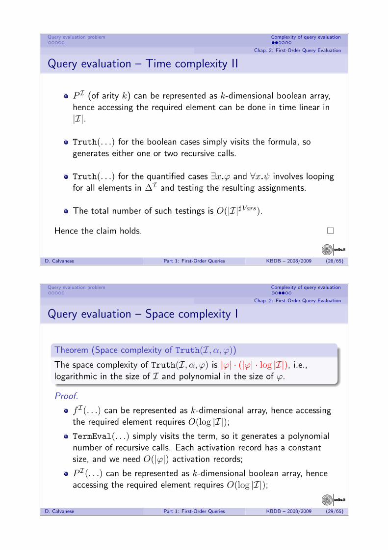
Query evaluation – Time complexity II
P I (of arity k) can be represented as k-dimensional boolean array,hence accessing the required element can be done in time linear in|I|.
Truth(. . .) for the boolean cases simply visits the formula, sogenerates either one or two recursive calls.
Truth(. . .) for the quantified cases ∃x.ϕ and ∀x.ψ involves loopingfor all elements in ∆I and testing the resulting assignments.
The total number of such testings is O(|I|]Vars).
Hence the claim holds.
D. Calvanese Part 1: First-Order Queries KBDB – 2008/2009 (28/65)
unibz.itunibz.it
Query evaluation problem Complexity of query evaluation
Chap. 2: First-Order Query Evaluation
Query evaluation – Space complexity I
Theorem (Space complexity of Truth(I, α, ϕ))
The space complexity of Truth(I, α, ϕ) is |ϕ| · (|ϕ| · log |I|), i.e.,logarithmic in the size of I and polynomial in the size of ϕ.
Proof.
fI(. . .) can be represented as k-dimensional array, hence accessingthe required element requires O(log |I|);
TermEval(. . .) simply visits the term, so it generates a polynomialnumber of recursive calls. Each activation record has a constantsize, and we need O(|ϕ|) activation records;
P I(. . .) can be represented as k-dimensional boolean array, henceaccessing the required element requires O(log |I|);
D. Calvanese Part 1: First-Order Queries KBDB – 2008/2009 (29/65)
unibz.itunibz.it
Query evaluation problem Complexity of query evaluation
Chap. 2: First-Order Query Evaluation
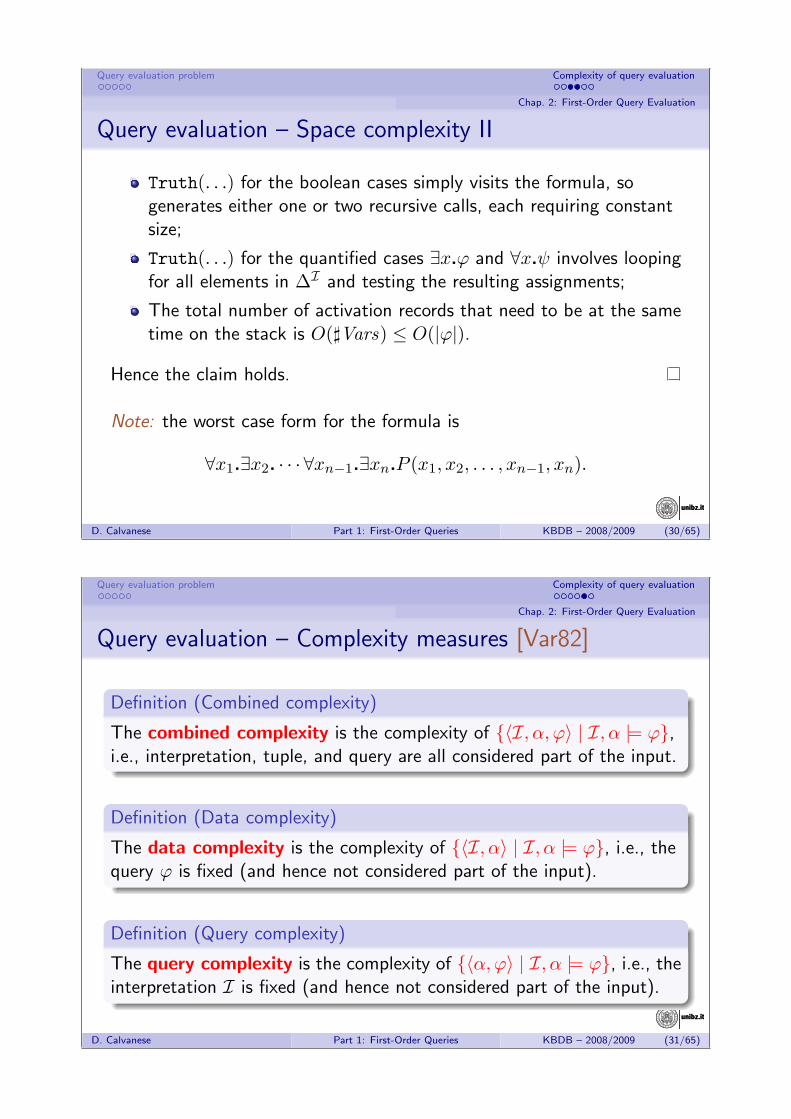
Query evaluation – Space complexity II
Truth(. . .) for the boolean cases simply visits the formula, sogenerates either one or two recursive calls, each requiring constantsize;
Truth(. . .) for the quantified cases ∃x.ϕ and ∀x.ψ involves loopingfor all elements in ∆I and testing the resulting assignments;
The total number of activation records that need to be at the sametime on the stack is O(]Vars) ≤ O(|ϕ|).
Hence the claim holds.
Note: the worst case form for the formula is
∀x1.∃x2. · · · ∀xn−1.∃xn.P (x1, x2, . . . , xn−1, xn).
D. Calvanese Part 1: First-Order Queries KBDB – 2008/2009 (30/65)
unibz.itunibz.it
Query evaluation problem Complexity of query evaluation
Chap. 2: First-Order Query Evaluation
Query evaluation – Complexity measures [Var82]
Definition (Combined complexity)
The combined complexity is the complexity of {〈I, α, ϕ〉 | I, α |= ϕ},i.e., interpretation, tuple, and query are all considered part of the input.
Definition (Data complexity)
The data complexity is the complexity of {〈I, α〉 | I, α |= ϕ}, i.e., thequery ϕ is fixed (and hence not considered part of the input).
Definition (Query complexity)
The query complexity is the complexity of {〈α,ϕ〉 | I, α |= ϕ}, i.e., theinterpretation I is fixed (and hence not considered part of the input).
D. Calvanese Part 1: First-Order Queries KBDB – 2008/2009 (31/65)

unibz.itunibz.it
Query evaluation problem Complexity of query evaluation
Chap. 2: First-Order Query Evaluation
Query evaluation – Combined, data, query complexity
Theorem (Combined complexity of query evaluation)
The complexity of {〈I, α, ϕ〉 | I, α |= ϕ} is:
time: exponentialspace: PSpace-complete — see [Var82] for hardness
Theorem (Data complexity of query evaluation)
The complexity of {〈I, α〉 | I, α |= ϕ} is:
time: polynomialspace: in LogSpace
Theorem (Query complexity of query evaluation)
The complexity of {〈α,ϕ〉 | I, α |= ϕ} is:
time: exponentialspace: PSpace-complete — see [Var82] for hardness
D. Calvanese Part 1: First-Order Queries KBDB – 2008/2009 (32/65)
unibz.itunibz.it
Evaluation of conjunctive queries Containment of conjunctive queries Unions of conjunctive queries
Chap. 3: Conjunctive Queries
Chapter III
Conjunctive Queries
D. Calvanese Part 1: First-Order Queries KBDB – 2008/2009 (33/65)
unibz.itunibz.it
Evaluation of conjunctive queries Containment of conjunctive queries Unions of conjunctive queries
Chap. 3: Conjunctive Queries
Outline
6 Evaluation of conjunctive queries
7 Containment of conjunctive queries
8 Unions of conjunctive queries
D. Calvanese Part 1: First-Order Queries KBDB – 2008/2009 (34/65)
unibz.itunibz.it
Evaluation of conjunctive queries Containment of conjunctive queries Unions of conjunctive queries
Chap. 3: Conjunctive Queries
Outline
6 Evaluation of conjunctive queries
7 Containment of conjunctive queries
8 Unions of conjunctive queries
D. Calvanese Part 1: First-Order Queries KBDB – 2008/2009 (35/65)
unibz.itunibz.it
Evaluation of conjunctive queries Containment of conjunctive queries Unions of conjunctive queries
Chap. 3: Conjunctive Queries
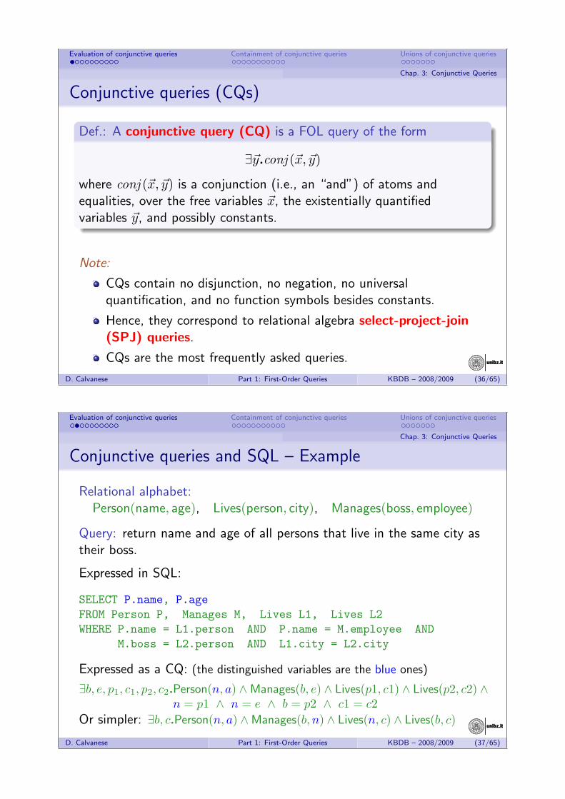
Conjunctive queries (CQs)
Def.: A conjunctive query (CQ) is a FOL query of the form
∃~y.conj (~x, ~y)
where conj (~x, ~y) is a conjunction (i.e., an “and”) of atoms andequalities, over the free variables ~x, the existentially quantifiedvariables ~y, and possibly constants.
Note:
CQs contain no disjunction, no negation, no universalquantification, and no function symbols besides constants.
Hence, they correspond to relational algebra select-project-join(SPJ) queries.
CQs are the most frequently asked queries.
D. Calvanese Part 1: First-Order Queries KBDB – 2008/2009 (36/65)
unibz.itunibz.it
Evaluation of conjunctive queries Containment of conjunctive queries Unions of conjunctive queries
Chap. 3: Conjunctive Queries
Conjunctive queries and SQL – Example
Relational alphabet:Person(name, age), Lives(person, city), Manages(boss, employee)
Query: return name and age of all persons that live in the same city astheir boss.
Expressed in SQL:
SELECT P.name, P.ageFROM Person P, Manages M, Lives L1, Lives L2WHERE P.name = L1.person AND P.name = M.employee AND
M.boss = L2.person AND L1.city = L2.city
Expressed as a CQ: (the distinguished variables are the blue ones)
∃b, e, p1, c1, p2, c2.Person(n, a) ∧Manages(b, e) ∧ Lives(p1, c1) ∧ Lives(p2, c2) ∧n = p1 ∧ n = e ∧ b = p2 ∧ c1 = c2
Or simpler: ∃b, c.Person(n, a) ∧Manages(b, n) ∧ Lives(n, c) ∧ Lives(b, c)
D. Calvanese Part 1: First-Order Queries KBDB – 2008/2009 (37/65)
unibz.itunibz.it
Evaluation of conjunctive queries Containment of conjunctive queries Unions of conjunctive queries
Chap. 3: Conjunctive Queries
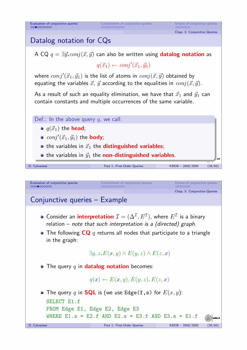
Datalog notation for CQs
A CQ q = ∃~y.conj (~x, ~y) can also be written using datalog notation as
q(~x1)← conj ′(~x1, ~y1)
where conj′(~x1, ~y1) is the list of atoms in conj (~x, ~y) obtained byequating the variables ~x, ~y according to the equalities in conj (~x, ~y).
As a result of such an equality elimination, we have that ~x1 and ~y1 cancontain constants and multiple occurrences of the same variable.
Def.: In the above query q, we call:
q(~x1) the head;
conj ′(~x1, ~y1) the body;
the variables in ~x1 the distinguished variables;
the variables in ~y1 the non-distinguished variables.
D. Calvanese Part 1: First-Order Queries KBDB – 2008/2009 (38/65)
unibz.itunibz.it
Evaluation of conjunctive queries Containment of conjunctive queries Unions of conjunctive queries
Chap. 3: Conjunctive Queries
Conjunctive queries – Example
Consider an interpretation I = (∆I , EI), where EI is a binaryrelation – note that such interpretation is a (directed) graph.
The following CQ q returns all nodes that participate to a trianglein the graph:
∃y, z.E(x, y) ∧ E(y, z) ∧ E(z, x)
The query q in datalog notation becomes:
q(x)← E(x, y), E(y, z), E(z, x)
The query q in SQL is (we use Edge(f,s) for E(x, y):
SELECT E1.fFROM Edge E1, Edge E2, Edge E3WHERE E1.s = E2.f AND E2.s = E3.f AND E3.s = E1.f
D. Calvanese Part 1: First-Order Queries KBDB – 2008/2009 (39/65)
unibz.itunibz.it
Evaluation of conjunctive queries Containment of conjunctive queries Unions of conjunctive queries
Chap. 3: Conjunctive Queries
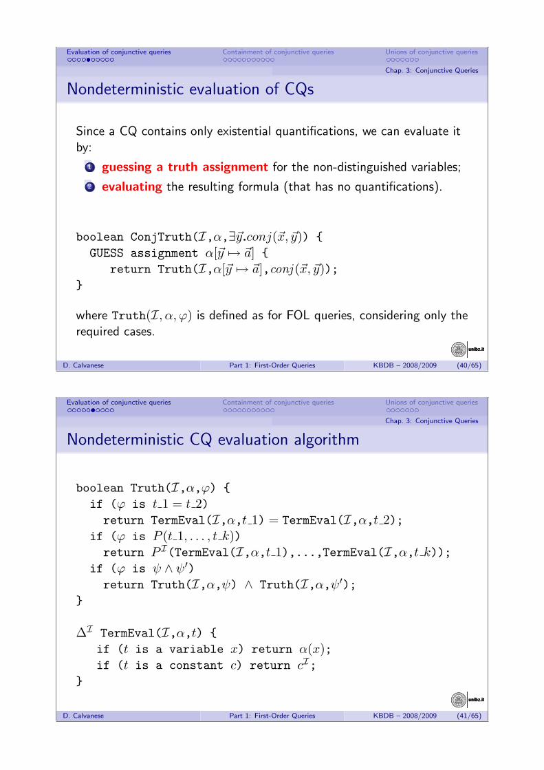
Nondeterministic evaluation of CQs
Since a CQ contains only existential quantifications, we can evaluate itby:
1 guessing a truth assignment for the non-distinguished variables;
2 evaluating the resulting formula (that has no quantifications).
boolean ConjTruth(I,α,∃~y.conj(~x, ~y)) {GUESS assignment α[~y 7→ ~a] {
return Truth(I,α[~y 7→ ~a],conj (~x, ~y));}
where Truth(I, α, ϕ) is defined as for FOL queries, considering only therequired cases.
D. Calvanese Part 1: First-Order Queries KBDB – 2008/2009 (40/65)
unibz.itunibz.it
Evaluation of conjunctive queries Containment of conjunctive queries Unions of conjunctive queries
Chap. 3: Conjunctive Queries
Nondeterministic CQ evaluation algorithm
boolean Truth(I,α,ϕ) {if (ϕ is t 1 = t 2)return TermEval(I,α,t 1) = TermEval(I,α,t 2);
if (ϕ is P (t 1, . . . , t k))return P I(TermEval(I,α,t 1),...,TermEval(I,α,t k));
if (ϕ is ψ ∧ ψ′)return Truth(I,α,ψ) ∧ Truth(I,α,ψ′);
}
∆I TermEval(I,α,t) {if (t is a variable x) return α(x);if (t is a constant c) return cI;
}
D. Calvanese Part 1: First-Order Queries KBDB – 2008/2009 (41/65)
unibz.itunibz.it
Evaluation of conjunctive queries Containment of conjunctive queries Unions of conjunctive queries
Chap. 3: Conjunctive Queries
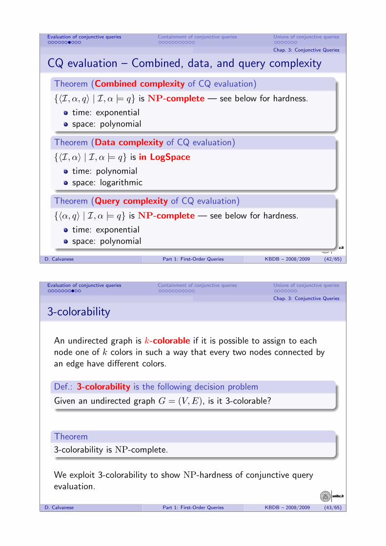
CQ evaluation – Combined, data, and query complexity
Theorem (Combined complexity of CQ evaluation)
{〈I, α, q〉 | I, α |= q} is NP-complete — see below for hardness.
time: exponentialspace: polynomial
Theorem (Data complexity of CQ evaluation)
{〈I, α〉 | I, α |= q} is in LogSpace
time: polynomialspace: logarithmic
Theorem (Query complexity of CQ evaluation)
{〈α, q〉 | I, α |= q} is NP-complete — see below for hardness.
time: exponentialspace: polynomial
D. Calvanese Part 1: First-Order Queries KBDB – 2008/2009 (42/65)
unibz.itunibz.it
Evaluation of conjunctive queries Containment of conjunctive queries Unions of conjunctive queries
Chap. 3: Conjunctive Queries
3-colorability
An undirected graph is k-colorable if it is possible to assign to eachnode one of k colors in such a way that every two nodes connected byan edge have different colors.
Def.: 3-colorability is the following decision problem
Given an undirected graph G = (V,E), is it 3-colorable?
Theorem
3-colorability is NP-complete.
We exploit 3-colorability to show NP-hardness of conjunctive queryevaluation.
D. Calvanese Part 1: First-Order Queries KBDB – 2008/2009 (43/65)

unibz.itunibz.it
Evaluation of conjunctive queries Containment of conjunctive queries Unions of conjunctive queries
Chap. 3: Conjunctive Queries
Reduction from 3-colorability to CQ evaluation
Let G = (V,E) be an undirected graph. We consider a relationalalphabet consisting of a single binary relation Edge and define:
An Interpretation: I = (∆I ,EdgeI) where:
∆I = {r, g, b}EdgeI = {(r, g), (g, r), (r, b), (b, r), (g, b), (b, g)}
A conjunctive query: Let V = {x1, . . . , xn}, then consider theboolean conjunctive query defined as:
qG = ∃x1, . . . , xn.∧
(xi,xj)∈EEdge(xi, xj) ∧ Edge(xj , xi)
Theorem
G is 3-colorable iff I |= qG.
D. Calvanese Part 1: First-Order Queries KBDB – 2008/2009 (44/65)
unibz.itunibz.it
Evaluation of conjunctive queries Containment of conjunctive queries Unions of conjunctive queries
Chap. 3: Conjunctive Queries
NP-hardness of CQ evaluation
The previous reduction immediately gives us the hardness for combinedcomplexity.
Theorem
CQ evaluation is NP-hard in combined complexity.
Note: in the previous reduction, the interpretation does not depend onthe actual graph. Hence, the reduction provides also the lower-boundfor query complexity.
Theorem
CQ evaluation is NP-hard in query (and combined) complexity.
D. Calvanese Part 1: First-Order Queries KBDB – 2008/2009 (45/65)

unibz.itunibz.it
Evaluation of conjunctive queries Containment of conjunctive queries Unions of conjunctive queries
Chap. 3: Conjunctive Queries
Outline
6 Evaluation of conjunctive queries
7 Containment of conjunctive queries
8 Unions of conjunctive queries
D. Calvanese Part 1: First-Order Queries KBDB – 2008/2009 (46/65)
unibz.itunibz.it
Evaluation of conjunctive queries Containment of conjunctive queries Unions of conjunctive queries
Chap. 3: Conjunctive Queries
Homomorphism
Let I = (∆I , P I , . . . , cI , . . .) and J = (∆J , PJ , . . . , cJ , . . .) be twointerpretations over the same alphabet (for simplicity, we consider onlyconstants as functions).
Def.: A homomorphism from I to Jis a mapping h : ∆I → ∆J such that:
h(cI) = cJ
h(P I(a1, . . . , ak)) = PJ (h(a1), . . . , h(ak))
Note: An isomorphism is a homomorphism that is one-to-one and onto.
Theorem
FOL is unable to distinguish between interpretations that are isomorphic.
Proof. See any standard book on logic.D. Calvanese Part 1: First-Order Queries KBDB – 2008/2009 (47/65)
unibz.itunibz.it
Evaluation of conjunctive queries Containment of conjunctive queries Unions of conjunctive queries
Chap. 3: Conjunctive Queries
Recognition problem and boolean query evaluation
Consider the recognition problem associated to the evaluation of a queryq of arity k. Then
I, α |= q(x1, . . . , xk) iff Iα,~c |= q(c1, . . . , ck)
where Iα,~c is identical to I but includes new constants c1, . . . , ck that
are interpreted as cIα,~ci = α(xi).
That is, we can reduce the recognition problem to the evaluationof a boolean query.
D. Calvanese Part 1: First-Order Queries KBDB – 2008/2009 (48/65)
unibz.itunibz.it
Evaluation of conjunctive queries Containment of conjunctive queries Unions of conjunctive queries
Chap. 3: Conjunctive Queries
Canonical interpretation of a (boolean) CQ
Let q be a conjunctive query ∃x1, . . . , xn.conj
Def.: The canonical interpretation Iq associated with q
is the interpretation Iq = (∆Iq , P Iq , . . . , cIq , . . .), where
∆Iq = {x1, . . . , xn} ∪ {c | c constant occurring in q},i.e., all the variables and constants in q;
cIq = c, for each constant c in q;
(t1, . . . , tk) ∈ P Iq iff the atom P (t1, . . . , tk) occurs in q.
Sometimes the procedure for obtaining the canonical interpretation iscalled freezing of q.
D. Calvanese Part 1: First-Order Queries KBDB – 2008/2009 (49/65)

unibz.itunibz.it
Evaluation of conjunctive queries Containment of conjunctive queries Unions of conjunctive queries
Chap. 3: Conjunctive Queries
Canonical interpretation of a (boolean) CQ – Example
Consider the boolean query q
q(c)← E(c, y), E(y, z), E(z, c)
Then, the canonical interpretation Iq is defined as
Iq = (∆Iq , EIq , cIq)
where
∆Iq = {y, z, c}EIq = {(c, y), (y, z), (z, c)}cIq = c
D. Calvanese Part 1: First-Order Queries KBDB – 2008/2009 (50/65)
unibz.itunibz.it
Evaluation of conjunctive queries Containment of conjunctive queries Unions of conjunctive queries
Chap. 3: Conjunctive Queries
Canonical interpretation and (boolean) CQ evaluation
Theorem ([CM77])
For boolean CQs, I |= q iff there exists a homomorphism from Iq to I.
Proof.“⇒” Let I |= q, let α be an assignment to the existential variables thatmakes q true in I, and let α̂ be its extension to constants. Then α̂ is ahomomorphism from Iq to I.
“⇐” Let h be a homomorphism from Iq to I. Then restricting h tothe variables only we obtain an assignment to the existential variablesthat makes q true in I.
D. Calvanese Part 1: First-Order Queries KBDB – 2008/2009 (51/65)
unibz.itunibz.it
Evaluation of conjunctive queries Containment of conjunctive queries Unions of conjunctive queries
Chap. 3: Conjunctive Queries
Canonical interpretation and (boolean) CQ evaluation
The previous result can be rephrased as follows:
(The recognition problem associated to) query evaluation can bereduced to finding a homomorphism.
Finding a homomorphism between two interpretations (aka relationalstructures) is also known as solving a Constraint SatisfactionProblem (CSP), a problem well-studied in AI – see also [KV98].
D. Calvanese Part 1: First-Order Queries KBDB – 2008/2009 (52/65)
unibz.itunibz.it
Evaluation of conjunctive queries Containment of conjunctive queries Unions of conjunctive queries
Chap. 3: Conjunctive Queries
Query containment
Def.: Query containment
Given two FOL queries ϕ and ψ of the same arity, ϕ is contained in ψ,denoted ϕ ⊆ ψ, if for all interpretations I and all assignments α wehave that
I, α |= ϕ implies I, α |= ψ
(In logical terms: ϕ |= ψ.)
Note: Query containment is of special interest in query optimization.
Theorem
For FOL queries, query containment is undecidable.
Proof.: Reduction from FOL logical implication.
D. Calvanese Part 1: First-Order Queries KBDB – 2008/2009 (53/65)
unibz.itunibz.it
Evaluation of conjunctive queries Containment of conjunctive queries Unions of conjunctive queries
Chap. 3: Conjunctive Queries
Query containment for CQs
For CQs, query containment q1(~x) ⊆ q2(~x) can be reduced to queryevaluation.
1 Freeze the free variables, i.e., consider them as constants.This is possible, since q1(~x) ⊆ q2(~x) iff
I, α |= q1(~x) implies I, α |= q2(~x), for all I and α; or equivalentlyIα,~c |= q1(~c) implies Iα,~c |= q2(~c), for all Iα,~c, where ~c are newconstants, and Iα,~c extends I to the new constants withcIα,~c = α(x).
2 Construct the canonical interpretation Iq1(~c) of the CQ q1(~c)on the left hand side . . .
3 . . . and evaluate on Iq1(~c) the CQ q2(~c) on the right hand side,i.e., check whether Iq1(~c) |= q2(~c).
D. Calvanese Part 1: First-Order Queries KBDB – 2008/2009 (54/65)
unibz.itunibz.it
Evaluation of conjunctive queries Containment of conjunctive queries Unions of conjunctive queries
Chap. 3: Conjunctive Queries
Reducing containment of CQs to CQ evaluation
Theorem ([CM77])
For CQs, q1(~x) ⊆ q2(~x) iff Iq1(~c) |= q2(~c), where ~c are new constants.
Proof.“⇒” Assume that q1(~x) ⊆ q2(~x).
Since Iq1(~c) |= q1(~c) it follows that Iq1(~c) |= q2(~c).
“⇐” Assume that Iq1(~c) |= q2(~c).
By [CM77] on hom., for every I such that I |= q1(~c) there exists ahomomorphism h from Iq1(~c) to I.
On the other hand, since Iq1(~c) |= q2(~c), again by [CM77] on hom., thereexists a homomorphism h′ from Iq2(~c) to Iq1(~c).The mapping h ◦h′ (obtained by composing h and h′) is a homomorphismfrom Iq2(~c) to I. Hence, once again by [CM77] on hom., I |= q2(~c).
So we can conclude that q1(~c) ⊆ q2(~c), and hence q1(~x) ⊆ q2(~x).D. Calvanese Part 1: First-Order Queries KBDB – 2008/2009 (55/65)
unibz.itunibz.it
Evaluation of conjunctive queries Containment of conjunctive queries Unions of conjunctive queries
Chap. 3: Conjunctive Queries
Query containment for CQs
For CQs, we also have that (boolean) query evaluation I |= q can bereduced to query containment.
Let I = (∆I , P I , . . . , cI , . . .).We construct the (boolean) CQ qI as follows:
qI has no existential variables (hence no variables at all);
the constants in qI are the elements of ∆I ;
for each relation P interpreted in I and for each fact(a1, . . . , ak) ∈ P I , qI contains one atom P (a1, . . . , ak) (note thateach ai ∈ ∆I is a constant in qI).
Theorem
For CQs, I |= q iff qI ⊆ q.
D. Calvanese Part 1: First-Order Queries KBDB – 2008/2009 (56/65)
unibz.itunibz.it
Evaluation of conjunctive queries Containment of conjunctive queries Unions of conjunctive queries
Chap. 3: Conjunctive Queries
Query containment for CQs – Complexity
From the previous results and NP-completenss of combined complexityof CQ evaluation, we immediately get:
Theorem
Containment of CQs is NP-complete.
Since CQ evaluation is NP-complete even in query complexity, theabove result can be strengthened:
Theorem
Containment q1(~x) ⊆ q2(~x) of CQs is NP-complete, even when q1 isconsidered fixed.
D. Calvanese Part 1: First-Order Queries KBDB – 2008/2009 (57/65)

unibz.itunibz.it
Evaluation of conjunctive queries Containment of conjunctive queries Unions of conjunctive queries
Chap. 3: Conjunctive Queries
Outline
6 Evaluation of conjunctive queries
7 Containment of conjunctive queries
8 Unions of conjunctive queries
D. Calvanese Part 1: First-Order Queries KBDB – 2008/2009 (58/65)
unibz.itunibz.it
Evaluation of conjunctive queries Containment of conjunctive queries Unions of conjunctive queries
Chap. 3: Conjunctive Queries
Union of conjunctive queries (UCQs)
Def.: A union of conjunctive queries (UCQ) is a FOL query of theform
∨
i=1,...,n
∃~yi.conj i(~x, ~yi)
where each conj i(~x, ~yi) is a conjunction of atoms and equalities withfree variables ~x and ~yi, and possibly constants.
Note: Obviously, each conjunctive query is also a of union ofconjunctive queries.
D. Calvanese Part 1: First-Order Queries KBDB – 2008/2009 (59/65)
unibz.itunibz.it
Evaluation of conjunctive queries Containment of conjunctive queries Unions of conjunctive queries
Chap. 3: Conjunctive Queries
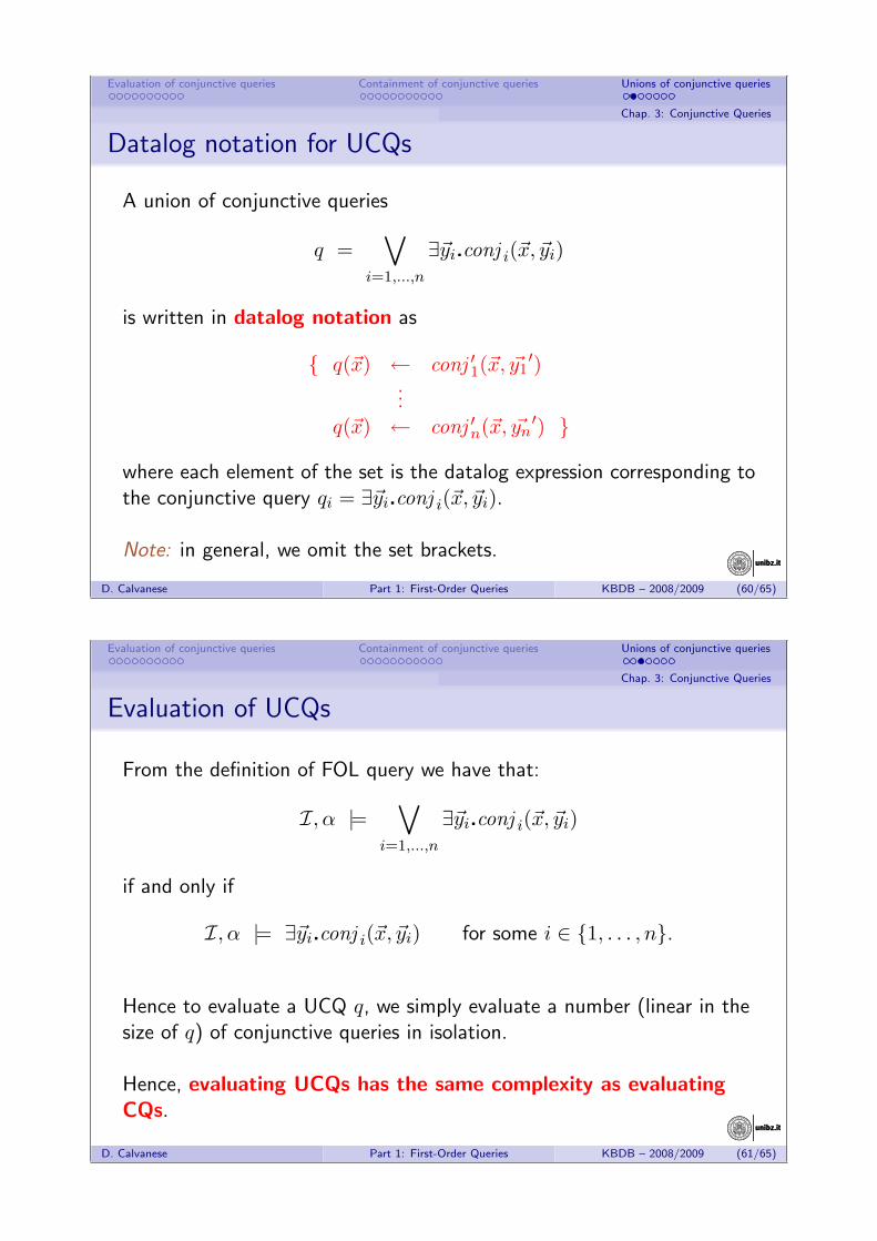
Datalog notation for UCQs
A union of conjunctive queries
q =∨
i=1,...,n
∃~yi.conj i(~x, ~yi)
is written in datalog notation as
{ q(~x) ← conj ′1(~x, ~y1′)
...q(~x) ← conj ′n(~x, ~yn′) }
where each element of the set is the datalog expression corresponding tothe conjunctive query qi = ∃~yi.conj i(~x, ~yi).
Note: in general, we omit the set brackets.
D. Calvanese Part 1: First-Order Queries KBDB – 2008/2009 (60/65)
unibz.itunibz.it
Evaluation of conjunctive queries Containment of conjunctive queries Unions of conjunctive queries
Chap. 3: Conjunctive Queries
Evaluation of UCQs
From the definition of FOL query we have that:
I, α |=∨
i=1,...,n
∃~yi.conj i(~x, ~yi)
if and only if
I, α |= ∃~yi.conj i(~x, ~yi) for some i ∈ {1, . . . , n}.
Hence to evaluate a UCQ q, we simply evaluate a number (linear in thesize of q) of conjunctive queries in isolation.
Hence, evaluating UCQs has the same complexity as evaluatingCQs.
D. Calvanese Part 1: First-Order Queries KBDB – 2008/2009 (61/65)

unibz.itunibz.it
Evaluation of conjunctive queries Containment of conjunctive queries Unions of conjunctive queries
Chap. 3: Conjunctive Queries
UCQ evaluation – Combined, data, and query complexity
Theorem (Combined complexity of UCQ evaluation)
{〈I, α, q〉 | I, α |= q} is NP-complete.
time: exponentialspace: polynomial
Theorem (Data complexity of UCQ evaluation)
{〈I, q〉 | I, α |= q} is in LogSpace (query q fixed).
time: polynomialspace: logarithmic
Theorem (Query complexity of UCQ evaluation)
{〈α, q〉 | I, α |= q} is NP-complete (interpretation I fixed).
time: exponentialspace: polynomial
D. Calvanese Part 1: First-Order Queries KBDB – 2008/2009 (62/65)
unibz.itunibz.it
Evaluation of conjunctive queries Containment of conjunctive queries Unions of conjunctive queries
Chap. 3: Conjunctive Queries
Query containment for UCQs
Theorem
For UCQs, {q1, . . . , qk} ⊆ {q′1, . . . , q′n} iff for each qi there is a q′j suchthat qi ⊆ q′j .
Proof.“⇐” Obvious.
“⇒” If the containment holds, then we have{q1(~c), . . . , qk(~c)} ⊆ {q′1(~c), . . . , q′n(~c)}, where ~c are new constants:
Now consider Iqi(~c). We have Iqi(~c) |= qi(~c), and henceIqi(~c) |= {q1(~c), . . . , qk(~c)}.By the containment, we have that Iqi(~c) |= {q′1(~c), . . . , q′n(~c)}. I.e.,there exists a q′j(~c) such that Iqi(~c) |= q′j(~c).
Hence, by [CM77] on containment of CQs, we have that qi ⊆ q′j .
D. Calvanese Part 1: First-Order Queries KBDB – 2008/2009 (63/65)

unibz.itunibz.it
Evaluation of conjunctive queries Containment of conjunctive queries Unions of conjunctive queries
Chap. 3: Conjunctive Queries
Query containment for UCQs – Complexity
From the previous result, we have that we can check{q1, . . . , qk} ⊆ {q′1, . . . , q′n} by at most k · n CQ containment checks.
We immediately get:
Theorem
Containment of UCQs is NP-complete.
D. Calvanese Part 1: First-Order Queries KBDB – 2008/2009 (64/65)
unibz.itunibz.it
Evaluation of conjunctive queries Containment of conjunctive queries Unions of conjunctive queries
Chap. 3: Conjunctive Queries
References
[CM77] A. K. Chandra and P. M. Merlin.
Optimal implementation of conjunctive queries in relational data bases.
In Proc. of the 9th ACM Symp. on Theory of Computing (STOC’77), pages77–90, 1977.
[KV98] P. G. Kolaitis and M. Y. Vardi.
Conjunctive-query containment and constraint satisfaction.
In Proc. of the 17th ACM SIGACT SIGMOD SIGART Symp. on Principles ofDatabase Systems (PODS’98), pages 205–213, 1998.
[Var82] M. Y. Vardi.
The complexity of relational query languages.
In Proc. of the 14th ACM SIGACT Symp. on Theory of Computing(STOC’82), pages 137–146, 1982.
D. Calvanese Part 1: First-Order Queries KBDB – 2008/2009 (65/65)