Laser Beam Profiling Using a Scanning Knife Edge

Technique

Submitted to:

Dr. Asloob Ahmad Mudassar

Submitted by:

Yasir Ali

M.Phil. Physics DPAM

PIEAS

Objective:

To investigate spatial characteristics of a He-Ne Laser using Scanning Knife Technique. To

measure the FWHM (full width half maximum) and 1/e2 diameters of the beam.

Introduction

In every laser application, whether in medical, industrial, laser printing, marking, welding

and cutting, or fiber optics, the beam profile provides valuable information for the most

efficient use of the laser. In laser industry it is desired to measure laser beam profile

before its use. The beam profile tells all about the beam’s spatial characteristics, which

in turn describe the distribution of beam’s energy, propagation, beam quality and utility

of the beam. By knowing beam profile we get information about shape of beam and can

improve it for our applications. Profiling is particularly helpful in building optical systems

for laser printers and fiber optic collimators. Until you know the beam profile, it is difficult

or even impossible to put the laser light to use.

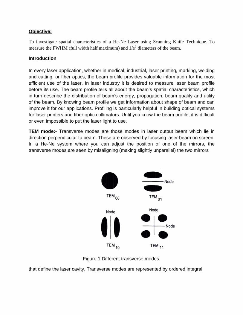
TEM mode:- Transverse modes are those modes in laser output beam which lie in

direction perpendicular to beam. These are observed by focusing laser beam on screen.

In a He-Ne system where you can adjust the position of one of the mirrors, the

transverse modes are seen by misaligning (making slightly unparallel) the two mirrors

Figure.1 Different transverse modes.

that define the laser cavity. Transverse modes are represented by ordered integral

subscripts appearing after the acronym TEM (Transverse Electromagnetic Mode),

specifying the number of nodes along the perpendicular axes. Some various transverse

modes are shown in figure.

What is Beam Profiling? Spatial characteristics describe the distribution of radiant energy across the wave front

of an optical beam i.e. in transverse to direction of beam. The radiation can be shown

as a plot of the relative intensity of points across a line that intersects projected path of

the beam. The most basic measurement of the beam’s irradiance is a single number

defining its width or diameter. Since optical beams do not actually have sharp physical

edges but it follow Gaussian distribution and energy is distributed to infinite distance,

there for beam width is made between two points that contain a major part of total

energy. For Gaussian, or at least approximately Gaussian beams, the common value

energy for this measurement is at the 1/e2. This is the point at which the beam’s power

is at 13.5% of the maximum height and diameter is measured at this point. Another

common measurement is at the full-width-half maximum (FWHM) level, where the

power drops to one half of the maximum.

Figure: Diameter (Full width) at half maximum or 1/e2 position from Gaussian

curve

Apparatus:-

He-Ne laser, emitting at wavelength of 632.8 nm;

A blade or knife, mounted on a stage which is capable of moving along the cross section of laser beam and having scale.

Photo detector to measure intensity.

Procedure:- In knife edge technique, a sharp blade is used to measure beam’s

diameter. Knife or sharp blade is fixed on a sliding translational slide which has some

scale for denoting position of knife.

Before starting scanning of knife, it is needed to measure background radiation. So we it

measured by blocking beam in front of detector and taking reading of detector. After

doing this, we started sliding the knife from position away from beam’s path such that

detector measured constant reading for initial three to four points. Gradually we moved

knife across the beam and measured intensity on detector. As knife was interrupting

beam, different readings were given by detector at different positions. We stopped

sliding when we noted that detector does not show any variation in measuring intensity

of radiation fallen on it.

This process was repeated several times and readings were taken.

Finding radius of beam:- We can find radius of the laser beam used in experiment

from the data obtained. First of all it is needed to remove background radiation. So at

first step, background radiation Ib is subtracted from measured intensity Im (I=Im – Ib).

Then intensity is converted into normalized intensity by dividing it by maximum of

intensity In=I/Imax. In is plotted against position of knife. The plot obtained is just like

Gaussian plot and radius of beam is obtained from it at 1/e2 position.

D1/2 = 13.24-5.4=7.84 µm or diameter D1= 15.68 µm.

Ib= 0.7 and X1=4.5 and X2 = 14 distance is in micrometers and intensity is in mV.

Position(µm) Intensity Position(µm) Intensity Position(µm) Intensity Position(µm) Intensity

4.5 3.33 7 3.21 9.5 1.91 12 0.79

5 3.33 7.5 3.04 10 1.64 12.5 0.72

5.5 3.33 8 2.82 10.5 1.35 13 0.7

6 3.32 8.5 2.58 11 1.11 13.5 0.7

6.5 3.3 9 2.25 11.5 0.93 14 0.7

D1/2= 14.51-6.5 = 8.01 µm or diameter D2= 16.02 µm.

Here Ib=0.25 , x1 =6.5 and x2 = 15.5 distance is in micrometers and intensity is in mV.

Position(µm) Intensity Position(µm) Intensity Position(µm) Intensity Position(µm) Intensity

6.5 2.31 9.0 2.08 11.5 1.3 14.0 0.3

7.0 2.29 9.5 1.93 12.0 1.04 14.5 0.26

7.5 2.28 10.0 1.85 12.5 0.81 15.0 0.25

8.0 2.26 10.5 1.74 13.0 0.59 15.5 0.25

8.5 2.19 11.0 1.58 13.5 0.42

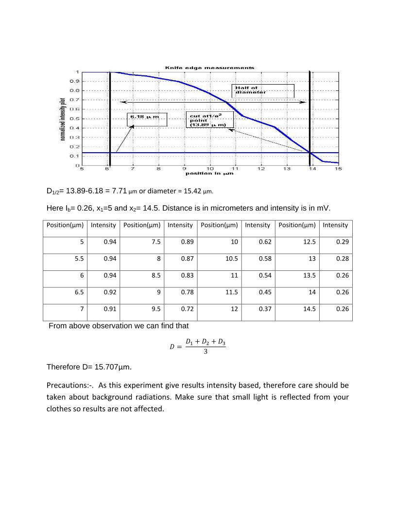
D1/2= 13.89-6.18 = 7.71 µm or diameter = 15.42 µm.

Here Ib= 0.26, x1=5 and x2= 14.5. Distance is in micrometers and intensity is in mV.

Position(µm) Intensity Position(µm) Intensity Position(µm) Intensity Position(µm) Intensity

5 0.94 7.5 0.89 10 0.62 12.5 0.29

5.5 0.94 8 0.87 10.5 0.58 13 0.28

6 0.94 8.5 0.83 11 0.54 13.5 0.26

6.5 0.92 9 0.78 11.5 0.45 14 0.26

7 0.91 9.5 0.72 12 0.37 14.5 0.26

From above observation we can find that

Therefore D= 15.707µm.

Precautions:-. As this experiment give results intensity based, therefore care should be

taken about background radiations. Make sure that small light is reflected from your

clothes so results are not affected.