Kinematics of curved flexible beam

University of South FloridaScholar Commons

Graduate Theses and Dissertations Graduate School

2006

Kinematics of curved flexible beamSaurabh JagirdarUniversity of South Florida

Follow this and additional works at: http://scholarcommons.usf.edu/etd

Part of the American Studies Commons

This Thesis is brought to you for free and open access by the Graduate School at Scholar Commons. It has been accepted for inclusion in GraduateTheses and Dissertations by an authorized administrator of Scholar Commons. For more information, please contact [email protected].

Scholar Commons CitationJagirdar, Saurabh, "Kinematics of curved flexible beam" (2006). Graduate Theses and Dissertations.http://scholarcommons.usf.edu/etd/2572

http://scholarcommons.usf.edu/?utm_source=scholarcommons.usf.edu%2Fetd%2F2572&utm_medium=PDF&utm_campaign=PDFCoverPages

http://scholarcommons.usf.edu/?utm_source=scholarcommons.usf.edu%2Fetd%2F2572&utm_medium=PDF&utm_campaign=PDFCoverPages

http://scholarcommons.usf.edu?utm_source=scholarcommons.usf.edu%2Fetd%2F2572&utm_medium=PDF&utm_campaign=PDFCoverPages

http://scholarcommons.usf.edu/etd?utm_source=scholarcommons.usf.edu%2Fetd%2F2572&utm_medium=PDF&utm_campaign=PDFCoverPages

http://scholarcommons.usf.edu/grad?utm_source=scholarcommons.usf.edu%2Fetd%2F2572&utm_medium=PDF&utm_campaign=PDFCoverPages

http://scholarcommons.usf.edu/etd?utm_source=scholarcommons.usf.edu%2Fetd%2F2572&utm_medium=PDF&utm_campaign=PDFCoverPages

http://network.bepress.com/hgg/discipline/439?utm_source=scholarcommons.usf.edu%2Fetd%2F2572&utm_medium=PDF&utm_campaign=PDFCoverPages

mailto:[email protected]

Kinematics of Curved Flexible Beam

by

Saurabh Jagirdar

A thesis submitted in partial fulfillment of the requirements for the degree of

Master of Science in Mechanical Engineering Department of Mechanical Engineering

College of Engineering University of South Florida

Major Professor: Craig P. Lusk, Ph.D. Rajiv Dubey, Ph.D. Autar K. Kaw, Ph.D.

Date of Approval: October 26, 2006

Keywords: Compliant mechanisms, Pseudo-rigid-body, Spherical, MEMS, Out of plane

© Copyright 2006, Saurabh Jagirdar

Dedication

Dedicated to my parents and my major professor.

Acknowledgement

I wish to express my gratitude to everyone who contributed to

making this thesis a reality. I must single out my professor Dr. Craig

P. Lusk who supported and guided me right from the beginning to

bring this thesis to fruition.

I also want to thank my supervisory committee Dr. Rajiv Dubey

and Dr Autar K. Kaw and all other professors for their encouragement

and guidance.

I am especially grateful to our department staff Ms Susan

Britten, Ms Shirley Tervort and Mr. Wes Frusher who helped me

through all the official procedures and setting up our compliant

mechanisms laboratory.

I thank Ms Cherine Chehab from the College of Engineering, USF

to edit and improve the format of the thesis.

I am indebted to Mr Prateek Asthana of CSEE, Dept, USF to help

me generate large number of input files by writing just one program.

This program saved me enormous amount of time that it would have

taken to generate them one by one.

I thank my friends and colleagues of the Mechanical engineering

department and other departments for making my life fun and also

helping me through various ways, a special reference to Daniel Vilceus

who continuously kept me pepped up with his sense of humour, Hari

Patel, John Daly, Shantanu Shevade, Aditya Bansal, Cesar Hernandez

and Son Ho.

I also thank my laboratory mates Joe, Alex, Diego, Sebastian,

Patricia and Issa for their help and support.

I am deeply indebted to my roommates Dr Apurva Panchal and

Phaninder Injeti for their patience to bear and take all my

eccentricities and help me through my tough times.

I once again thank the Mechanical Engineering Department., the

College of Engineering and University of South Florida, Tampa Florida.

i

Table of Contents

List of Tables ii List of Figures iii Abstract vi 1. Introduction 1

1.1 Scope 2 1.2 Background 4 1.3 Roadmap 15

2. Methodology and Model Development 16 2.1 Correspondence between spherical and planar PRBMs 16 2.2 Kinematics of compliant circular arc 18 2.3 Spherical kinematics of the pseudo-rigid-body model 21 2.4 Spherical loading condition analogous to planar vertical end load 23

3. Finite Element Analysis (FEA) 24

4. Parametric Approximation of the Curved Beam’s Deflection Path 33

5. Results and Discussion 40

6. Conclusion 50

References 51

Appendices 56 Appendix A Spherical Triangles and Napier Rules 57 Appendix B Manual for FEA 62 Appendix C Algorithms to Find γ 100 Appendix D Summary 119

ii

List of Tables

Table 1: Spherical PRBM 119 Table 2: Planar PRBM 120

iii

List of Figures

Figure 1: A PRBM for a cantilever beam with a vertical end load

(Howell 2001) 7 Figure 2: Planar Mechanism with sliders moving on perpendicular

straight lines 9 Figure 3: Spherical mechanism with sliders moving on

perpendicular circular arcs 10 Figure 4: Geodesics 11 Figure 5: Parallel transport (Henderson 1998) 13 Figure 6: Parallel transport along the same longitude 14 Figure 7: Relationship between existing planar PRBM and the

spherical PRBM developed in this work 17 Figure 8: Reference frames describing the motion of the end of a

compliant circular cantilever 20 Figure 9: The pseudo-rigid-body model of the compliant curved

beam 22 Figure 10: Path followed by beam the dotted line from Q to Q’’ 25 Figure 11: Reference frames used to model the spherical

mechanism and its planar equivalent 26 Figure 12: Cross-section of beam for various aspect ratios 29 Figure 13: Finite element model 30 Figure 14: Deflection of curved segment 35 Figure 15: Deflection of PRBM 37

iv

Figure 16: Final position of beam from fixed end α, v/s input displacement β 41

Figure 17: Deflection of beam about neutral axis, θ0,v/s input

displacement β 41 Figure 18: γ v/s Arc-lengths showing various colors for aspect

ratios 42 Figure 19: CΘ v/s Arc-lengths showing various colors for aspect ratios43 Figure 20: Θmax v/s Arc-lengths showing various colors for aspect

ratios 43 Figure 21: γ v/s Arc-lengths, for 200 load-steps of input

displacement 45 Figure 22: CΘ v/s Arc-lengths, for 200 load-steps of input

displacement 46 Figure 23: Θmax v/s Arc-lengths, for 200 load-steps of input

displacement 47 Figure 24: Trend-line of γ, for aspect ratio 0.1 48 Figure 25: Trend-line of γ, for aspect ratio 0.4 48 Figure 26: Trend-line of γ, for aspect ratio 0.7 49 Figure 27: Spherical triangles 57 Figure 28: Five parts arranged in order of occurrence 58 Figure 29: Spherical right triangle 59 Figure 30: Five parts for PRBM right spherical triangle 60 Figure 31: Activating Graphical User Interface (GUI) 62 Figure 32: Limiting the GUI options to structural preferences 63 Figure 33: Adding or defining new element types 64

v

Figure 34: Beam elements 65 Figure 35: Defining real constants for respective elements 66 Figure 36: Inputting area and moment of inertia values to elements 67 Figure 37: Defining material properties 68 Figure 38: Creating key-points on work-plane through GUI 69 Figure 39: Creating key-points using command line 70 Figure 40: Pan, zoom, rotate 71 Figure 41: Defining of orthogonal triad at beam end 72 Figure 42: Creating lines 73 Figure 43: Creating arcs 74 Figure 44: Meshing 75 Figure 45: Mesh attributes for line 76 Figure 46: Allocating specific material to mesh (elements) 77 Figure 47: Selecting analysis type 78 Figure 48: Large displacement analysis selected 79 Figure 49: Equation chosen solvers 80 Figure 50: Applying loads to the beam 81 Figure 51: Solve 82 Figure 52: During solve 83 Figure 53: Output 84 Figure 54: To get the log-file 85

vi

Kinematics of Curved Flexible Beam

Saurabh Jagirdar

ABSTRACT

Compliant mechanism theory permits a procedure called rigid-

body replacement, in which two or more rigid links of the mechanism

are replaced by a compliant flexure with equivalent motion. Methods

for designing flexure with equivalent motion to replace rigid links are

detailed in Pseudo-Rigid-Body Models (PRBMs). Such models have

previously been developed for planar mechanisms. This thesis

develops the first PRBM for spherical mechanisms.

In formulating this PRBM for a spherical mechanism, we begin by

applying displacements are applied to a curved beam that cause it to

deflect in a manner consistent with spherical kinematics. The motion of

the beam is calculated using Finite Element Analysis. These results are

analyzed to give the PRBM parameters. These PRBM parameters vary

with the arc length and the aspect ratio of the curved beam.

1

1. Introduction

Mechanisms have been defined as “mechanical devices for

transferring motion and/or force from a source to an output” (Erdman

et al. 2001). Mechanisms form an important part of how our modern

society interacts with the world, whether it is the steering wheel, the

computer keyboard, or even the handle of a door. Most mechanisms

are systems of levers, cams and gears, which move and rotate, and

which have rigid parts. Compliant mechanisms are mechanisms that

“gain some or all of their ability to move from the deflection of flexible

segments” (Salamon 1989). In compliant mechanisms, individual parts

not only move and rotate, but also undergo elastic deformations in

response to the forces which are imposed on them. Some common

compliant mechanisms are binder clips, paper clips, backpack latch,

lid, nail-clippers, etc. Compliant mechanisms can have improved

performance, lower costs and greater potential functional integration

when compared with rigid-body mechanisms (Her 1986, Sevak and

McLarman 1974).

2

1.1 Scope

Compliant mechanism theory permits a procedure called rigid-

body replacement, in which two or more rigid links of the mechanism

are replaced by a compliant flexure with equivalent motion (Howell

2001). Methods for designing flexure with equivalent motion to replace

rigid links are detailed in Pseudo-Rigid-Body Models (PRBMs). In many

texts, (Boettama and Roth, Mc Carthy 2000), rigid body analysis of

synthesis techniques have been classified as planar, spherical and

spatial according to the type of vector algebra used to describe the

mechanisms. In a planar mechanism, the path of any single part of a

link lies in a plane and in a spherical mechanism, the path of any

single part of a link lies on the surface of a sphere.

Numerous PRBMs have been developed for planar mechanisms

by Midha et al (1992, 2000), Howell and Midha (1994a, 1994b, 1995)

Saxena and Kramer (1998), and Dado (2001) and used in applications

such as Microelectromechanical Systems (MEMS) (Baker et al. 2000,

Hubbard 2005, Ananthasuresh et al, 1993, Ananthasuresh and Kota

1996, Jensen et al. 1997, Salmon et al. 1996 and Kota et al. 2001),

prosthetics (Guerinot et al. 2004), clutches (Roach et al. 1998, Crane

et al. 2004), micro-bearings (Cannon et al. 2005), constant-force

mechanisms (Millar et al. 1996), parallel mechanisms (Derderian et al.

1996), and bi-stable mechanisms (Jensen et al. 1999) and used in

3

various other applications like thermal and electrical actuating

mechanisms for MEMS (Brocket and Stokes (1991) and Saggere and

Kota (1997)). Thus, extensive research has been done on planar

compliant mechanisms using PRBMs.

A prime advantage of compliant mechanisms is the part count

reduction, that is, flexures can replace rigid links and reduce the

number of joints (Howell 2001). This plays a significant role in the

fabrication of MEMS. In MEMS design, the increase in the number of

joints directly increases the complexity to manufacture MEMS. (Howell

2001). Compliant mechanisms also have increased precision, increased

reliability, reduced weight and reduced maintenance (Howell 2001).

These advantages make compliant mechanisms ideal for MEMS design

and hence the applications for MEMS using compliant mechanisms are

abundant.

The PRBM concept has been particularly fruitful in the design of

surface micro-machined MEMS. Surface micromachining is less

expensive and more versatile than alternative forms of fabrication

(Howell 2001). For these reasons much of current MEMS research is

devoted to this technique. But MEMS designs, fabricated by surface

micro-machining are limited to moving back-and-forth and side-to-side

(two dimensional motion) i.e. surface micro-machined devices are

essentially flat (or in-plane or planar). For applications that need a

4

micro mechanism that rotates out of the plane of fabrication with an

in-plane rotational input, or that rotates spatially about a point,

existing planar compliant mechanisms are not suitable. Given that all

current PRBMs relate compliant mechanisms to planar rigid-body

mechanisms, we are led to ask is it possible to derive PRBMs that

relate compliant mechanisms to spherical rigid-body mechanisms. No

such PRBMs have been developed for spherical mechanisms. It is

anticipated that the description of compliant spherical mechanisms

with spherical motion will simplify the design of MEMS with out of

plane motion.

In this thesis, the first PRBM for a spherical compliant

mechanism is developed. The kinematics of a curved flexure with the

equivalent of a vertical end load is studied and a spherical PRBM for a

curved cantilever beam is developed by approximating the motion of

the compliant flexure as an equivalent rigid-body mechanism.

1.2 Background

The motion of rigid-body mechanisms can be analyzed with

matrix algebra (McCarthy 2000) or other techniques and more

sophisticated techniques are required for spherical mechanisms than

planar mechanisms. The analysis of the motion of compliant

mechanisms, on the other hand, usually requires the solution of

5

differential equations, which describe the physics of an infinitely thin

section of the mechanism (Frisch Fay 1962). Because the terms planar

and spherical describe the gross motion of objects of finite size, it is

not obvious a priori when or if these terms apply to compliant

mechanisms. However, a compliant mechanism may be termed as

planar or spherical mechanism when the solution of its governing

differential equations can be reasonably approximated with rigid-body

mathematical techniques i.e. matrix algebra. To convert the solution

method of a compliant mechanism from a differential equation

approach to an algebraic approach, a number of assumptions and

specifications need to be made. The differential equation gives

information about the relationships of a continuous series of points in

the mechanism; the algebraic equation gives information about a few

specific points. Thus, the transition requires the specification of the

points of interest, typically the ends of the flexible segment. The

solution to the differential equations requires that boundary conditions,

i.e. information about applied loads and displacements, be specified

(Howell 2001). Thus, the conversion to an algebraic solution is valid

only for the specific loading conditions. These restrictions usually are

placed on loading directions rather than magnitudes (Howell 2001). A

validated and accurate identification between a spherical compliant

6

mechanism and a rigid-body mechanism with equivalent motion at the

points of interest is a spherical PRBM.

The PRBM consists of diagrams and equations describing the

flexible member and gives a rigid-link equivalent of the compliant

mechanism which has the same motion and flexibility for a known

range of motion and to a known mathematical tolerance. A PRBM can

be used to perform analysis (i.e. given a compliant flexure, its motion

can be found by treating it as the rigid body) or design (given a

particular desired motion, a rigid body mechanism that performs the

motion can be found, and the PRBM can be used to convert that rigid-

body mechanism into a compliant mechanism). The creation of a PRBM

entails steps beyond the typical mathematical analysis of motion of the

compliant segment. These additional steps are necessary to find a

simple and accurate rigid-body approximation of the motion of the

compliant segment. Once that rigid-body approximation has been

identified, it is optimized and validated so that its range of applicability

and level of error is known and acceptable. This identification step

requires proposing a topology for the rigid-body mechanism, i.e.

specification of the number of links and joints. The optimization and

validation of steps involve using a numerical optimization routine that

insures that the rigid body approximation has a tolerable error (less

than 0.5%) over as large a range of motion as possible. The creation

7

of such PRBMs is justified because they are easy to use in design and

because the use of the PRBM in connection with rigid-body synthesis

techniques produces compliant mechanism configurations that are

unlikely to be produced in any other way. An example of this approach

is the PRBM for a straight cantilever beam with vertical end load

(Howell 2001), which associates motion of a compliant flexure with a

rigid-link mechanism as shown in Figure 1. Figure 1(a) shows a

straight cantilever beam subjected to a vertical end load F. Figure 1(b)

shows the pseudo-rigid-body equivalent of the straight cantilever

beam. The distance from the fixed end to the beam end in the x-

direction is a, the distance from the fixed end to the beam end in the

y-direction is b, length of the straight beam is l , Θ is the pseudo-

rigid-body angle and γ is the characteristic radius factor. The angle of

inclination of the beam at the beam end is given by θ0.

(a) Compliant (b) PRBM equivalent

Figure 1: A PRBM for a cantilever beam with a vertical end load (Howell 2001)

8

The co-ordinates of the beam end of the compliant beam are

given in terms of the PRB angle, Θ, as:

)]cos1(1[ Θ−−= γla (1.1)

Θ= sinlb γ (1.2)

Where γ=0.85 for a vertical end load.

The relationship between Θ and θ0 is given by:

Θ= 24.10θ (1.3)

These relations are accurate to less than 0.5% error for

Θ<64.3o.

These rigid-body link equations help us to calculate the precise

motion of the compliant cantilever i.e. for a given pseudo-rigid-body

angle, Θ, we can calculate the final co-ordinates of the beam end from

the fixed end, a in the x-direction and b in the y-direction. We can also

calculate the angle of inclination of the beam, θ0.

There are analogies between planar mechanisms and spherical

mechanisms that make it possible to develop a spherical PRBM from

the planar PRBM of a cantilever with a vertical end load. A key

component of the analogies between planar and spherical mechanisms

is that straight lines in planar mechanisms become great circles or

circular arcs in spherical mechanisms (Chiang 1992). Also, angles

between lines become angles between planes (containing great

9

circles). For example, a planar mechanism may have an input in the y-

direction and an output in the x-direction as shown in Figure 2.

Figure 2: Planar Mechanism with sliders moving on perpendicular straight

lines

The analogous spherical mechanism will travel on two

perpendicular circular arcs Y-direction (equivalent of y direction) and

an output in the X-direction (equivalent of x-direction) as shown in

Figure 2 as shown in Figure 3.

10

Figure 3: Spherical mechanism with sliders moving on perpendicular circular

arcs

Note that spherical mechanisms whose size is very small

compared to the radius of the sphere closely approximate planar

mechanisms. In fact, spherical kinematics is identical to the planar

kinematics in the limiting case when the radius of the sphere is

infinite.

We are also motivated by the ideas that relate planes and

spheres such as the stereographic projections used by cartographers

to represent a spherical earth on a flat map or the mathematical

identification between the complex plane and the Riemann sphere

(Frankel 1997). Let us divide the sphere S just like the earth into

latitudes, longitudes and equator. All longitudes and the equator are

great circles (WordNet 2001). Great circles are circles that have the

11

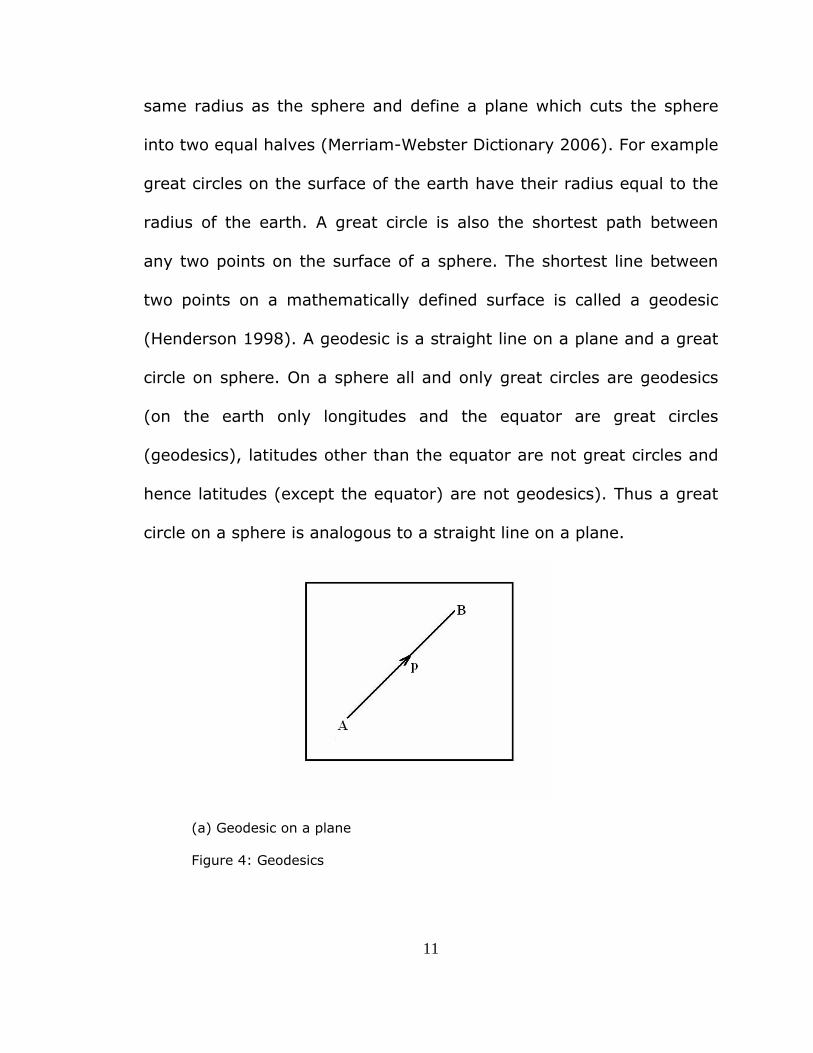
same radius as the sphere and define a plane which cuts the sphere

into two equal halves (Merriam-Webster Dictionary 2006). For example

great circles on the surface of the earth have their radius equal to the

radius of the earth. A great circle is also the shortest path between

any two points on the surface of a sphere. The shortest line between

two points on a mathematically defined surface is called a geodesic

(Henderson 1998). A geodesic is a straight line on a plane and a great

circle on sphere. On a sphere all and only great circles are geodesics

(on the earth only longitudes and the equator are great circles

(geodesics), latitudes other than the equator are not great circles and

hence latitudes (except the equator) are not geodesics). Thus a great

circle on a sphere is analogous to a straight line on a plane.

(a) Geodesic on a plane

Figure 4: Geodesics

12

(b) Geodesic on a sphere

Figure 4: (Continued)

Figure 4(a) shows the shortest path p between A and B, on a

plane. Figure 4(b) shows the shortest path p between A and B, on a

sphere. Moreover, on a sphere because “straight” lines are great

circles (curved), there are no parallel lines. ‘Parallelism’ does not exist,

that is, all great circles intersect on a sphere. Parallel transport on a

sphere is an analogous concept to parallel lines on a plane. Lines that

intersect a geodesic (great circles) with the same angle are parallel

transports (Henderson 1998).

13

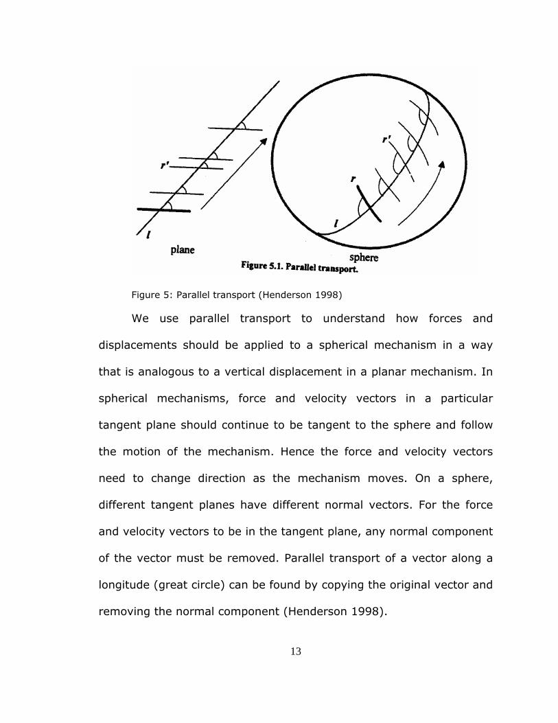
Figure 5: Parallel transport (Henderson 1998)

We use parallel transport to understand how forces and

displacements should be applied to a spherical mechanism in a way

that is analogous to a vertical displacement in a planar mechanism. In

spherical mechanisms, force and velocity vectors in a particular

tangent plane should continue to be tangent to the sphere and follow

the motion of the mechanism. Hence the force and velocity vectors

need to change direction as the mechanism moves. On a sphere,

different tangent planes have different normal vectors. For the force

and velocity vectors to be in the tangent plane, any normal component

of the vector must be removed. Parallel transport of a vector along a

longitude (great circle) can be found by copying the original vector and

removing the normal component (Henderson 1998).

14

A vector m is parallel transported along a longitude to obtain a

vector n as shown in Figure 6.

Figure 6: Parallel transport along the same longitude

All longitudes make the same angle with the equator (geodesic)

(Henderson 1998). Thus, all longitudes are parallel transports of each

other. At any point in the northern hemisphere, all vectors pointing to

the North Pole will lie on longitudes, thus any vector in the northern

hemisphere and pointing towards the North Pole is a parallel transport

of any other such vector. Thus, a northward-pointing force-vector on

the equator of a sphere can be parallel transported to a vector pointing

north at any other point on the sphere. A vector pointing north on a

sphere is analogous to a vertical force in a plane.

15

1.3 Roadmap

This chapter has presented background on PRBMs and spherical

kinematics, Later chapters describe, how the spherical PRBM is

modeled, analyzed and validated. Chapter 2 describes the analogy

between planar PRBM and a spherical PRBM. It also gives the

nomenclature and topology for the spherical PRBM. Chapter 3

describes the finite element model and how the displacements were

applied to the model. Chapter 4 describes how the data was used to

obtain the values for the PRBM parameters given in the second

chapter. Chapter 5 describes the results obtained for different aspect

ratios, b/h and arc lengths, λ. Chapter 6 is the conclusion based on the

results.

16

2. Methodology and Model Development

2.1 Correspondence between spherical and planar PRBMs

Mechanisms whose joint axes are parallel to each other are

known as planar mechanisms (Chiang 1992). In planar compliant

mechanisms, this characteristic is usually achieved by designing

straight cantilevers (flexures) that, at each point along their length,

are most flexible about parallel lines and considerably more rigid in

other directions. Mechanisms whose joint axes intersect at a point are

spherical mechanisms (Chiang 1992). In spherical compliant

mechanisms, this characteristic can be achieved by designing curved

cantilevers (flexures) that, at each point along the arc, are most

flexible about lines that point to the centre of the sphere. In both kinds

of mechanisms it is necessary that the length (arc-length) of flexure

be much greater than the width of the beam (flexure), and the width

of the beam to be larger than its thickness.

It is hypothesized that a flexure which is a long, thin circular arc

will move in a manner consistent with spherical kinematics when

loaded appropriately. The process of obtaining the PRBM for a

17

spherical compliant mechanism is similar to planar compliant

mechanism.

Figure 7: Relationship between existing planar PRBM and the spherical PRBM

developed in this work

The spherical compliant mechanism and its rigid body

counterpart are derived from the planar mechanism by making

straight lines curved. There is a correspondence principle between

spherical PRBMs and planar PRBMs. The correspondence principle is

that when small angle assumption is used for spherical arcs. i.e. the

arc length is much smaller than the radius of the sphere, the spherical

PRBM becomes identical to planar PRBM. To emphasize the

relationship between lines and arcs, the lengths in planar model are

denoted with Roman letters, and the equivalent arcs in the spherical

model are denoted with the Greek letter equivalents. For example the

18

arc length, β, that appears in some formulas for spherical

mechanisms, can be related to the planar length, b. Thus, using small

angle approximation.

b→==

βββ

sin,1cos

Where b is the planar equivalent of the arc β. Similarly a and

l are the planar equivalent of arcs α and λ respectively.

Additionally, similar terminology is used in planar and spherical

PRBMs, for angles between lines (arcs) such as Θ, θ0, and for ratios

such as γ and Cθ. These variables do not change in the small angle

case. In the planar case, the deflected angle of beam end, θ0, is about

an axis normal to the plane. Similarly, in the spherical case, the

deflection of the beam end, θ0, is about an axis normal to the tangent

plane to the sphere at the beam end.

2.2 Kinematics of compliant circular arc

The kinematics of the compliant circular cantilever, PQ, is

described by using a series of co-ordinate frames, as shown in Figure

8. The fixed end of the curved cantilever beam is denoted as P and

free end of the beam as Q. Let S be a sphere whose center is defined

by O frame and the frames A, B, C and D are always on the surface of

19

the sphere. The position and orientation of the co-ordinate frames are

related as follows:

The O frame is a fixed frame that locates the center of the

sphere.

The A frame is a frame that locates the beam end Q, in un-

deflected co-ordinates with neutral axis of beam at Q is parallel to the

a3 direction and the a1 direction is outward radial vector through the

beam end.

The B frame is a frame that locates the deflected position of the

beam end Q in the x-z plane (analogous to the translation in the x-

direction in the planar model).

The C frame is a moving frame that describes movement of

beam end Q in the b2-b1 plane rotating about point O (analogous to

the translation in the y-direction in the planar model).

The D frame is a moving frame at the same position as the C

frame and tracks the deflection of the beam end about the radial axis

through the beam end (analogous to the deflection about the z-axis in

the planar model).

20

Figure 8: Reference frames describing the motion of the end of a compliant

circular cantilever

The frames are described by the matrices A, B, C and D, where

the columns of the matrix are the basis vectors. The transformations

relating the frames are given by:

⎥⎥⎥

⎦

⎤

⎢⎢⎢

⎣

⎡==

100010001

}]{},{},[{ 321 aaaA

AaRAbbbB ),ˆ()cos(0)sin(

010)sin(0)cos(

}]{},{},[{ 2321 Φ−=⎥⎥⎥

⎦

⎤

⎢⎢⎢

⎣

⎡

Φ−Φ−

Φ−Φ−==

21

BbRBcccC ),ˆ(1000)cos()sin(0)sin()cos(

}]{},{},[{ 3321 βββββ

=⎥⎥⎥

⎦

⎤

⎢⎢⎢

⎣

⎡ −==

CcRCdddD ),ˆ()cos()sin(0)sin()cos(0

001}]{},{},[{ 01

00

00321 θθθθθ =

⎥⎥⎥

⎦

⎤

⎢⎢⎢

⎣

⎡−==

The transformations relating the frames are given by:

AaRbRcRD ),ˆ(),ˆ(),ˆ( 2301 Φ−= βθ

Thus the motion of the cantilever beam is described by the

parameter Φ=λ-α, β and θ0 which are analogous to planar parameters

l-a, b and θ0, respectively which are shown in Figure 1.

2.3 Spherical kinematics of the pseudo-rigid-body model

Now by analogy to the planar PRBM, in the spherical PRBM, Θ is

defined as the pseudo-rigid-body angle of the beam end about the

characteristic-pivot (pseudo-pivot) and γ is defined as the ratio of the

arc length from the beam end to the pseudo-pivot to the entire arc

length λ of the beam. The value of γ is chosen so that the motion of

the beam end closely approximates the motion of the compliant beam.

The details of selecting the value of γ are explained in chapter 4.

Thus the proposed topology for the pseudo-rigid-body model is

shown in Figure 9.

22

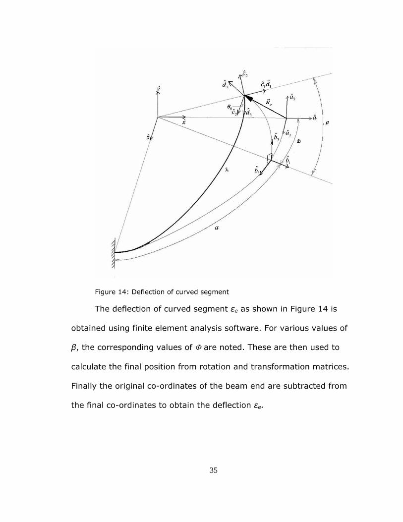
Figure 9: The pseudo-rigid-body model of the compliant curved beam

The relationships for α and β in terms of γ and Θ are obtained

using Napier rules for right spherical triangle (Spiegel, 1968). The right

spherical triangle in Figure 9 has sides γλ, η, and β (See Appendix A)

where

λγαη )1( −−=

Thus we find η as a function of γλ and Θ

)cos(tantan)90tan(tan)90sin(

1 Θ=

−=Θ−− γλη

γλη

(2.1)

23

And α is obtained as

)cos(tantan)1()1(

1 Θ+−=

+−=− γλλγα

ηλγα (2.2)

Also β is obtained as a function of γλ and Θ

)sin(sinsinsinsinsin

1 Θ=

Θ=− γλβ

γλβ

(2.3)

2.4 Spherical loading condition analogous to planar vertical end

load

Based on the discussion in chapter 2, the spherical equivalent of

a vertical end load is northward-pointing end-load. An important

distinction between planar and spherical loading conditions is that the

planar load direction is constant; the spherical load direction must

change. A vertical end load in the planar case always points upward,

on a sphere there is no such one direction to which the load vector

points. The direction of the force vector should change as the

mechanism moves along the curvature of the sphere. In practice the

change requires that any component of force in the direction normal to

the sphere must be removed, perhaps by addition of load bearing

members in the mechanism. Thus, at any other point on the sphere

the vector initiating from that point and pointing towards the North

Pole imitates a vertical end load in planar case.

24

3. Finite Element Analysis (FEA)

To deduce the accurate motion of the beam going through

spherical motion the beam is modeled in a FEA software package. The

parametric angle co-efficient, CΘ, the characteristic radius factor, γ,

and the parameterization limit, Θmax, are obtained from the results of

the FEA model. A major challenge in building the model in FEA

package is to apply loads on the beam such that there is no reaction

load at the fixed end, P, (see Figure 10) and the free end, Q, of curved

cantilever beam moves in a manner consistent with spherical

kinematics. For this study we focus on the motion of the beam

(kinematics), the reaction loads will be studied in later work.

Development of the model is a paradox because the load

direction depends on the displacement of the beam end, and the

displacement of the beam end depends on the load direction. Thus, to

ensure that there is no reaction load at the fixed end, P, we need to

know the path (dotted line shown in Figure 10) followed by the beam

end. The path followed is an arc on the sphere from the A frame (un-

deflected position Q) to the C or D frame (final position Q’’).

25

Figure 10: Path followed by beam the dotted line from Q to Q’’

When the beam PQ is taken as fixed at P, the A-frame of

reference is fixed. The motion of the beam can also be described in the

B-frame of reference such that the end Q of the beam is allowed to

move in the b1-b2 plane. As a consequence of this the end P, of the

beam now moves in the b1-b3 plane, that is, the beam undergoes

spherical motion such that the ends P and Q move on orthogonal great

26

circles. To illustrate clearly, the comparison with the planar case is

shown.

(a) Planar Fixed reference frame (b) Planar Moving reference frame

(c) Spherical Fixed reference frame (d) Spherical Moving reference frame

Figure 11: Reference frames used to model the spherical mechanism and its

planar equivalent

We can see from Figure 11(a) and 11(c) that if an input is given

at the free end Q, the output obtained when the beam is fixed at P is a

displacement at Q. On the other hand, in Figure 11(b) and 11(d) an

27

input is given at Q and the output is obtained at P. As we see from

Figure 11, the difference between the fixed frame of reference and

moving frame of reference is the location of the output displacements.

In the planar case, when an input displacement of b is given the

output obtained is o=l-a in both the fixed frame of reference, shown in

Figure 11(a), and the moving frame of reference Figure 11(b). In the

spherical case, when an input displacement of β is given, the output

obtained is Φ=λ-α in both the fixed frame of reference, shown in

Figure 11(c), and the moving frame of reference, shown in Figure

11(d). Thus, the mechanisms are equivalent to each other and only

the frame of reference has changed. It proves convenient to analyze

the behavior of the flexible curved beam in a FEA model built to mimic

the moving frame. In this frame of reference, we apply displacement

loads at Q and measure the output displacement at P. The fixed frame

of reference is the A frame in Figure 10 In order to get the spherical

frame B.

When the B-frame is observed in a moving frame of reference it

coincides with the A-frame for all northward-pointing input

displacements. The initial position is such that both the ends of the

beam are in the b1-b3 plane. An input of displacement angle, β, is

applied to the beam end Q. The motion of Q is a circular arc in b1-b2

plane. The output obtained is the displacement angle Φ (about the y-

28

axis of the O frame) observed at the other end P of the beam. The

motion of this beam end, P, is a circular arc that lies in the b1-b3 plane.

The mechanism shown in 11(d) is modeled in FEA software package.

The ANSYS version 10.0, (ANSYS, 2006) FEA package was used.

A major aspect of modeling in ANSYS is that it does not take inputs or

outputs with respect to units. Hence the model itself has to be built in

a single system of consistent units. Since this is a ‘kinematic’ model,

the factors expected to affect the results would be dimensions of the

curved beam and Modulus of Elasticity. Here the model dimensions

were defined in millimetres (mm) and the modulus of elasticity in

Newton per square millimetre (N/mm2).

In this model we take the length of the rigid beam OP

=1000mm, the radius of the arc PQ=1000mm. The Q end of the beam

is always in the X-Y plane and its initial position for all arc-lengths of

PQ, is Q(1000,0,0). The initial position of the end P varies for different

arc-lengths and is given by P(R*cos(arclength),0,R*sin(arclength)).

Where R is the radius of the arc (sphere) =1000mm and

arclength is the angle created by the arc to the centre in radians.

The mechanism is modeled such that the circular segment PQ is

highly compliant and the straight segment OP is highly rigid. This is

done by maintaining the modulus of elasticity of the compliant circular

segment at 300N/mm2 and that of the rigid straight segment at

29

300,000 N/mm2. Various aspect ratios of the beam are obtained by

varying the cross-section of the beam that is if an aspect ratio of 0.1 is

desired then the thickness (or height h) of the beam is 1/10 th of the

width b. When aspect ratio of the beam is 1 the beam has a square

cross-section of sides 50mm, for successive values of aspect ratio the

sides vary accordingly to obtain a rectangular cross-section of width b

and height h given by h=aspect ratio * b as shown in Figure 12.

Figure 12: Cross-section of beam for various aspect ratios

This model is then meshed to define elements and nodes.

Displacement loads are applied according to the boundary conditions

described below.

To apply the boundary conditions for the above model we denote

the displacements in x, y and z directions by UX, UY and UZ and

30

rotations about x, y and z by ROTX, ROTY and ROTZ. Points O and P

lie on the rigid straight segment and hence they are made to stay in

the x-z plane and allowed to rotate about y-axis of O frame. The point

O fixes the structure in space and hence all other degrees of freedom

are constrained. The point Q is the end of the curved segment and

hence it is made to lie in the x-y plane.

The boundary conditions applied to the finite element model shown in

Figure 13 are:

Point O UX=0, UY=0, UZ=0, ROTX=0, ROTZ=0.

Point P UY=0,

Point Q UZ=0, ROTZ=β, ROTX=0, ROTY=0.

Figure 13: Finite element model

31

Rotational displacement loads, β, were applied at the Q end of

the beam and analysis was conducted. For various inputs of β we get

corresponding outputs of Φ=λ-α. The deflection θ0 of the neutral axis

of the beam at beam end (that moves in b1-b2 plane) about the radial

axis of the beam at the same beam end is also obtained as an output.

The deflection of the beam is calculated from the rotation matrix

generated by a pre-defined triad at the Q end of the beam.

Thus these outputs are noted for various inputs and this

simulation is repeated for varying:

a) Initial arc length λ b) Cross-section of the curved flexible

beam. The results from FEA model were used to calculate the

parametric angle co-efficient, Cθ, the characteristic radius factor, γ and

θ0max. See Appendix C for a visual manual to conduct one simulation. A

log file generated from one analysis (simulation) is then obtained from

the file menu. This log file is then edited with new values of the

parameters (aspect ratio and arc-length) and subsequently run in

ANSYS by using an input command. Simulations were run for arc-

lengths ranging from angle of 4 degrees to 112 degrees in increments

of 2 degrees and for each arclength aspect ratios varying from 0.1 to 1

with increments of 0.1. The input displacement, β, is given such that it

is equal to the angle created by the respective arc-length, that is, if an

32

arc-length of 90 degrees is to be analyzed then an input displacement

of 90 degrees is applied.

33

4. Parametric Approximation of the Curved Beam’s Deflection

Path

We follow Howell’s method (Howell 2001) for developing our

parametric approximation of the curved beam’s deflection path. An

acceptable value for the characteristic radius factor, γ, may be found

by first determining the maximum acceptable percentage error in

deflection. The value of γ that would allow the maximum pseudo-rigid-

body angle, Θ, while still satisfying the maximum error constraint is

then determined. The problem may be formally stated as follows: Find

the value of the characteristic radius factor γ which maximizes the

pseudo-rigid-body angle, Θ, where Θ for a spherical mechanism is

derived from Napier Rules. For right spherical triangle whose sides are

γλ, η, and β, and Θ is the angle between γλ and η it can be shown that:

Θ= cottan)]-(1-sin[ βγλα (See Appendix A)

where

φλα −=

to get

⎥⎦

⎤⎢⎣

⎡−−

=Θ −

)]1(sin[tantan 1

γλαβ

(4.1)

34

Equation (4.1) is valid for β< 90ο.

⎥⎥⎥

⎦

⎤

⎢⎢⎢

⎣

⎡=Θ −

γληγλ

β

cottansin

sintan 1

(4.2)

Equation (4.2) is applicable for all values of β (See Appendix-

A), and is subject to the parametric constraint

(4.3)

where error/εe is the relative deflection error, and εe for a spherical

mechanism is defined as the vector difference of deflected position of

the flexible curved segment and the original un-deflected position.

)0()/(/)( maxmax Θ<Θ<≤=Θ forerrorerrorg ee εε

35

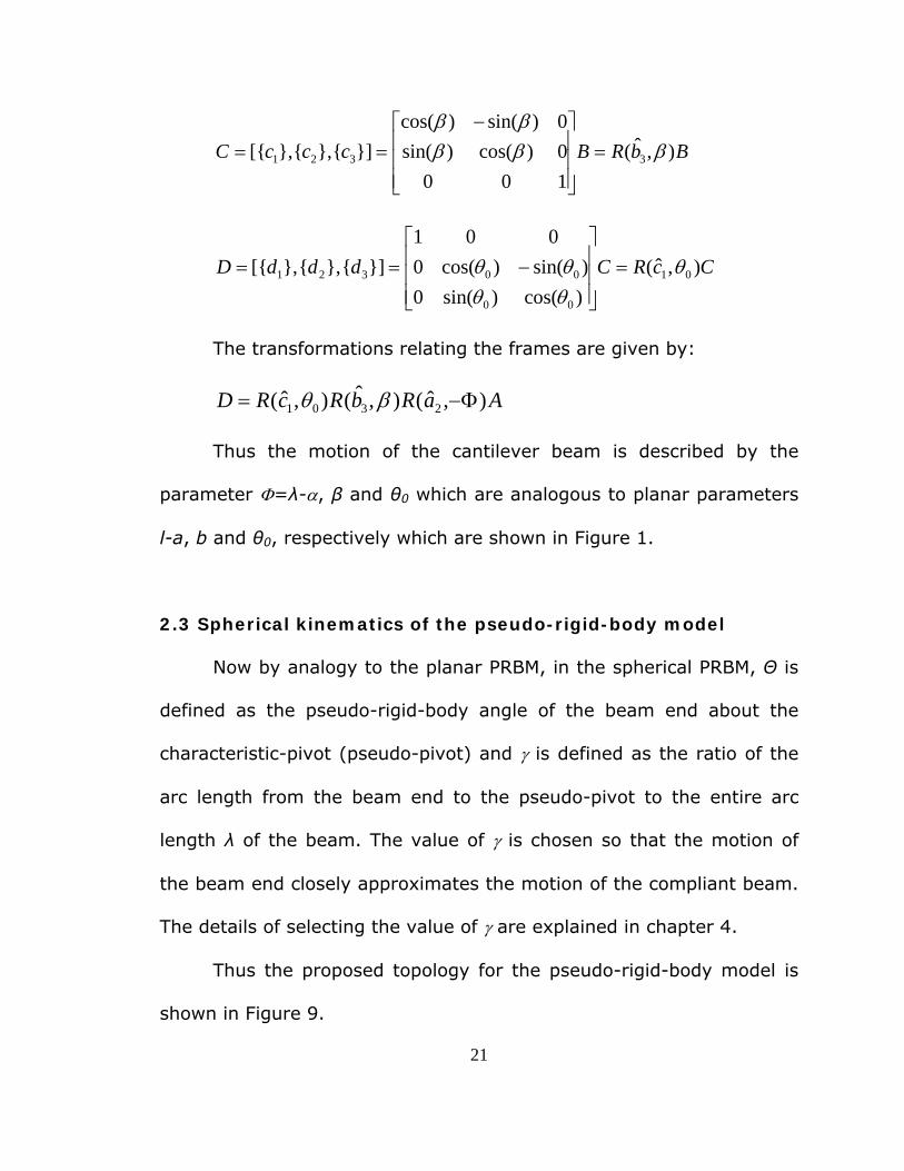
Figure 14: Deflection of curved segment

The deflection of curved segment εe as shown in Figure 14 is

obtained using finite element analysis software. For various values of

β, the corresponding values of Φ are noted. These are then used to

calculate the final position from rotation and transformation matrices.

Finally the original co-ordinates of the beam end are subtracted from

the final co-ordinates to obtain the deflection εe.

36

⎥⎥⎥

⎦

⎤

⎢⎢⎢

⎣

⎡ −=

⎥⎥⎥

⎦

⎤

⎢⎢⎢

⎣

⎡−

⎥⎥⎥

⎦

⎤

⎢⎢⎢

⎣

⎡

⎥⎥⎥

⎦

⎤

⎢⎢⎢

⎣

⎡

−−−

−−

⎥⎥⎥

⎦

⎤

⎢⎢⎢

⎣

⎡ −=

φββ

φβ

φφ

φφββββ

εsincos

sin1coscos

001

001

)cos(0)sin(010

)sin(0)cos(

1000cossin0sincos

er

(4.4)

to get

(4.5)

and the deflection for the PRBM, εa, is given by the vector difference of

deflected position of the PRBM and the original un-deflected position of

the beam end Q.

⎥⎥⎥

⎦

⎤

⎢⎢⎢

⎣

⎡ −=

⎥⎥⎥

⎦

⎤

⎢⎢⎢

⎣

⎡=

φββ

φβ

εεε

εsincos

sin1coscos

ez

ey

ex

er

37

Figure 15: Deflection of PRBM

The vector difference between the estimated deflected position

of PRBM and the original un-deflected position of beam end, Q, is

calculated using the following transformations.

From Figure 15 we have rRarrr

−=ε

and rRR rr= where R is the rotation of the vector rr about the axis

mr through angle Θ (Lai, Rubin and Krempl, 1993).

38

)(sincos).)(cos1(),,( rmrmrmrmR rrrrrrrrr×Θ+Θ+Θ−=Θ

where,

⎥⎥⎥

⎦

⎤

⎢⎢⎢

⎣

⎡=

λγ

λγ

ˆsin0

ˆcosmr

and ⎥⎥⎥

⎦

⎤

⎢⎢⎢

⎣

⎡=

001

rr

which reduces to

⎥⎥⎥

⎦

⎤

⎢⎢⎢

⎣

⎡

Θ−Θ

Θ+Θ−==

)cos1(ˆsinˆcossinˆsin

cos)cos1(ˆcos2

λγλγλγ

λγrRR rr

Therefore,

⎥⎥⎥

⎦

⎤

⎢⎢⎢

⎣

⎡

Θ−Θ

−Θ+Θ−=

)cos1(ˆsinˆcossinˆsin

1cos)cos1(ˆcos2

λγλγλγ

λγε ar

(4.6)

error is simply defined as the vector difference between the final

positions of the curved flexible segment and the pseudo-rigid body

model.

39

The error in the deflection is calculated as

( ) ( ) ( )[ ] 2/1222azezayeyaxexaeerror εεεεεεεε −+−+−=−=

rr

(4.7)

A parameter relative error, error/εe is defined to help in

comparing with the planar flexible segment.

e

ae

e

errorε

εεε

r

rr

r−

= (4.8)

The value of the angular deflection of the beam’s end, θ0, at the

point at which the error equals or exceeds an acceptable amount, is

the maximum angular deflection of the beam’s end, or the

parameterization limit Θmax.

40

5. Results and Discussion

For a given value of aspect ratio, h/b, and arc-length, λ, one can

find a value of characteristic radius factor, γ and parametric angle co-

efficient, CΘ that best approximates the motion (position and

orientation of beam at various input displacements) using the

techniques described in the previous chapter.

For example for h/b=1, and λ=90ο, the final displacement of beam from

the fixed end, α, and the rotation θ0 are found for a given input

displacement of β. They are plotted against β as shown in Figure 16

and Figure 17.

41

Figure 16: Final position of beam from fixed end α, v/s input displacement β

Figure 17: Deflection of beam about neutral axis, θ0,v/s input displacement β

42

Then the values of γ and CΘ that gives the minimum relative

error (0.05%) for the largest range of different guess of γ are found for

maximum range of motion.

CΘ is the parametric angle co-efficient, defined as the ratio of the

maximum range of motion obtained, Θmax, in the pseudo-rigid body

model to the ratio of the deflection of the beam about the neutral

axis,θ0.

The γ and CΘ obtained for all the simulations of various aspect

ratios and arc lengths are plotted in Figure 18 and Figure 19 and in

Figure 20 the maximum range of motion for the PRBM for the

respective values of γ and CΘ.

Figure 18: γ v/s Arc-lengths showing various colors for aspect ratios

43

Figure 19: CΘ v/s Arc-lengths showing various colors for aspect ratios

Figure 20: Θmax v/s Arc-lengths showing various colors for aspect ratios

44

These are graphs that are plotted for simulations which were run

to obtain outputs at every one degree of the input displacement,

β, that is, if the beam was given a total input displacement of 90

degrees then 90 load-steps of one degree were solved. As a

consequence not enough data points were obtained when the total

input displacement, β was a small value, for example, if the beam was

given a total input displacement of just 10 degrees then only 10 load-

steps were solved. Thus, the algorithm to process the outputs obtained

from the simulations failed to process the data for arc-lengths ranging

from 4 to 14 because the total input displacement, β, is given such that

it is equal to the arc-length. Hence, the number of data points at an

arc-length, were limited to the value of arc-length in degrees, that is,

only 4 data points were obtained for an arc-length of 4 degrees.

Moreover, from the graphs it can be seen that there is a lot of

‘bouncing’ that is there is a ‘noise’ in the data. This clearly indicates

that more data points are required to capture the behavior of the

curved beams.

Based on the inference of these graphs the simulations were re-run

such that 200 load-steps are solved irrespective of the value of the

input displacement, that is, for an input displacement of 4 degrees the

beam was analyzed at an input displacement, β, of every 4/200

degrees. These simulations were run for aspect ratios h/b=0.1, 0.4

45

and 0.7. These are then again plotted as shown in Figure 21, Figure 22

and Figure 23.

Figure 21: γ v/s Arc-lengths, for 200 load-steps of input displacement

46

Figure 22: CΘ v/s Arc-lengths, for 200 load-steps of input displacement

47

Figure 23: Θmax v/s Arc-lengths, for 200 load-steps of input displacement

From Figures 21, 22 and 23 we see that there is no ‘bouncing’ or

‘noise’ in the data, smooth curves are obtained. It is observed that this

data is suitable to approximate the motion of the beam. An equation is

fitted to the curve for the characteristic radius factor γ, and can be

used to approximate the motion of a curved beam with the equivalent

of vertical end load. A trend-line of second order polynomial for arc-

lengths ranging from 16 to 112 is fit individually for aspect ratios

h/b=0.1, 0.4 and 0.7 and their equations are shown in Figure 24,

Figure 25 and Figure 26.

48

y = -7E-06x2 + 0.0002x + 0.848

0.770.780.79

0.80.810.820.83

0.840.850.86

0 20 40 60 80 100 120

Arclength, λ

Cha

ract

eris

tic ra

dius

fact

or, γ

Figure 24: Trend-line of γ, for aspect ratio 0.1

y = -7E-06x2 + 0.0001x + 0.8507

0.77

0.78

0.79

0.8

0.81

0.82

0.83

0.84

0.85

0.86

0 20 40 60 80 100 120

Arclength, λ

Cha

ract

eris

tic ra

dius

fact

or,


49

y = -6E-06x2 - 1E-04x + 0.8576

0.770.780.790.8

0.810.820.830.840.850.860.87

0 20 40 60 80 100 120

Arclength, λ

Cha

ract

eris

tic ra

dius

fact

or, γ


Thus, at a given aspect ratio h/b and arc-length λ of curved

beam we can substitute the values in the respective equation to find

the corresponding characteristic radius factor γ for the spherical PRBM

that best approximates the motion of the curved flexible beam.

50

6. Conclusion

The first Pseudo-Rigid-Body Model (PRBM) for spherical

mechanisms has been developed. The kinematics of a compliant

curved beam and its rigid body equivalent were described. The

procedure for analyzing the curved compliant beams in a FEM program

was developed. Pseudo-rigid body parameters were calculated from

FEA results. These parameters are the characteristic radius factor, γ,

the parametric angle co-efficient CΘ and the parameterization limit

Θmax. These values approach the values found in the planar case for

small arc lengths, λ.

51

References

1) Ananthasuresh, G.K., 1994, “A New Design Paradigm for Micro-

Electro-Mechanical Systems and Investigations on the Compliant Mechanism Synthesis,” Ph.D. dissertation, University of Michigan, Ann Arbor, MI.

2) Ananthasuresh, G. K., and Kota, S., 1995, “Designing of

Compliant Mechanisms,” Mechanical Engineering, Vol. 117, No.11, pp. 93-96.

3) Ananthasuresh, G.K., Kota, S., and Gianchandani, Y., 1994, “A

Methodical Approach to the Design of Compliant Micro-mechanisms,” Solid-State Sensor and Actuator Workshop, Hilton Head Island, SC, pp. 189-192.

4) ANSYS 10.0, ANSYS University Advanced Release 10.0. 5) Baker, M.S., Lyon, S.M., and Howell L.L., 2000, “A Linear

Displacement Bistable Micromechanism,” Proceedings of the 26th Biennial Mechanisms and Robotics Conference, 2000 ASME Design Engineering Technical Conferences, DETC2000/MECH-14119.

6) Boettama.O. and Roth, B., 1979, Theoretical Kinematics Dover,

New York. 7) Brocket W. R. and Stokes A., 1991 “On the Synthesis of

Compliant Mechanisms” 8) Cannon J.R., Lusk C.P. and Howell, L.L., 2005 “Compliant

Rolling-Contact Element Mechanisms”, ASME Mechanisms and Robotics Conference 2005.

9) Chiang, C. H., 1992, Spherical kinematics in contrast to planar

kinematics, National Taiwan University, Taipei, Taiwan, Mech Mach Theory v 27 n 3 May 1992 p 243-250.

52

10) Crane, N.B., Howell L.L., and Weight, B. L., 2000, “Design and Testing of a Compliant Floating-Opposing Arm (FOA) Centrifugal Clutch,” Proceedings of 8th International Power Transmission and Gearing Conference, 2000 ASME Design Engineering Technical Conferences DETC2000/PTG-14451.

11) Dado M. H, 2001 “Variable Parametric Pseudo-Rigid Body Model

for Large Deflection Beams with End Loads” International Journal of Non-linear Mechanics, 2001.

12) Derderian, J.M., 1996, “The Pseudo-Rigid Body Model Concept

and its Application to Micro Compliant Mechanisms,” M.S. thesis, Brigham Young University, Provo, UT.

13) Erdman, A.G., and Sandor, G.N., 1997, Mechanism Design:

Analysis and Synthesis, Vol. 1, 3rd Ed., Prentice Hall, Upper Saddle River, NJ.

14) Frankel, T., 1997 The Geometry of Physics, Cambridge

University Press, pp21-22. 15) Frisch-Fay, R., 1962, Flexible Bars, Butterworth, Washington DC. 16) Guerinot A. E., Magleby S. P., and Howell, L. L., 2004

“Preliminary Design Concepts for Compliant Mechanism Prosthetic Knee Joints”, ASME Mechanisms and Robotics Conference 2004.

17) Her, I., and Midha, A., 1987, “A Compliance Number Concept for

Compliant Mechanisms, and Type Synthesis.” Journal of Mechanisms, Transmissions, and Automation in Design, Trans. ASME, Vol. 109, No. 3, pp. 348-355.

18) Her, I., 1986, “Methodology for Compliant Mechanisms Design,”

Ph.D dissertation, Purdue University, West Lafayette, IN. 19) Henderson, D. W., 1998 Differential Geometry, Prentice Hall

Upper Saddle River, NJ. 20) Hill, T.C., and Midha, A., 1990, “A graphical user-driven Newton-

Raphson Technique for use in the Analysis and Design of Compliant Mechanisms.” Journal of Mechanical Design, Trans ASME, Vol. 112, No. 1, pp. 123-130.

53

21) Howell L. L., 2001, Compliant Mechanisms, John Wiley and Sons, Inc, NY.

22) Howell, L. L., 1991, “The Design and Analysis of Large Deflection

Members in Compliant Mechanisms,” M.S. thesis, Purdue University, West Lafayette, IN.

23) Howell, L. L., and Midha, A., 1993, “Compliant Mechanisms,”

Section 9.10 in Modern Kinematics: Developments in the Last Forty Years, (A. G. Erdman, ed.), Wiley, New York, pp. 422-428.

24) Howell, L. L., and Midha, A., 1994, “The development of Force

Deflection Relationships,” Machine elements and Machine Dynamics: Proceedings of the 1994 ASME Mechanisms conference, DE-Vol. 71, pp. 501-508.

25) Howell, L. L., and Midha, A., 1995, “Parametric Deflection

Approximations for End-Loaded, Large Deflection Beams in Compliant Mechanisms,” Journal of Mechanical Design, ASME, Vol. 117, No.1, pp. 156-165.

26) Howell, L. L., and Midha, A ., 1995, “Determination of the

Degrees of Freedom of Compliant Mechanisms using the Pseudo-Rigid Body Model Concept,” Proceedings of the 9th World Congress on the Theory of Machines and Mechanisms, Milano, Italy, Vol. 22, pp. 1537-1541.

27) Howell, L.L., Rao, S.S., and Midha, A., 1994, “The Reliability

Based Optimal Design of a Bistable Compliant Mechanism,” Journal of Mechanical Design, Trans. ASME, Vol. 116, No. 4, pp. 1115-1121.

28) Howell, L.L., and Midha, A., 1995, “Parametric Deflection

Approximations for End-Loaded, Large-Deflection Beams in Compliant Mechanisms,” Journal of Mechanical Design, Trans. ASME, Vol. 71, pp. 156-165.

29) N.B. Hubbard, L.L. Howell, 2005 “Design and Characterization of

a Duel-stage, Thermally Actuated Nanopositioner”, Journal of Micromechanics and Microengineering, 2005.

54

30) Jensen, B.D., Howell L.L., Gunyan, D.B., and Salmon, L.G., 1997, “The Design and Analysis of Compliant MEMS Using the Pseudo-Rigid-Body Model,” Micromechanical Systems (MEMS), at the 1997 ASME International Mechanical Engineering Congress and Exposition, DSC-Vol. 62, pp. 119-126.

31) Jensen, B.D., Howell L.L., and Salmon, L.G., 1999, “Design of

Two-Link, In-plane, Bi-stable Compliant Micro-mechanisms,” Journal of Mechanical Design, Trans. ASME, Vol. 121, No. 3, pp. 93-96.

32) Lai, M.W., Rubin, D, Krempl, E, 1993 Introduction to Continuum

Mechanics 3rd ed Pergamon, Pr. 33) Merriam-Webster Dictionary, 2006, Merriam-Webster Online.

“http://www.m-w.com/cgi-bin/dictionary?book=Dictionary&va=great%20circle”.

34) Midha, A., Her, I., and Salamon, B.A., 1992, “A Methodology for

Compliant Mechanisms Design, Part I: Introduction and Large-Deflection Analysis,” in Advances in Design Automation, D.A Hoeltzel, ed., 18th ASME Design Automation Conference, DE-Vol. 44-2, pp. 29-38.

35) Midha, A., and Howell, L.L., 2000, “Limit Positions of Compliant

Mechanism using the Pseudo-rigid body Model”, Mechanism and Machine Theory, Vol. 35, No. 1, pp. 99-115.

36) McCarthy, J., 2000 Geometric Design of Linkages Springer, NY. 37) Millar A. J., Howell L L and Leonard J N, 1996 “Design and

Evaluation of Compliant Constant Force Mechanisms”. 38) Roach, G.M., and Howell, L. L., 2000, “Compliant Overrunning

clutch with centrifugal Throw out,” U.S. patent 6,148,979, Nov 21.

39) Salamon, B.A., 1989, “Mechanical Advantage Aspects in

Compliant Mechanisms Design,” in Advances in Design Automation, D.A Hoeltzel, ed., 18th ASME Design Automation Conference, DE-Vol44-2, pp. 47-51.

55

40) Saggere L. and Kota S.,1997 “Synthesis of Distributed Compliant Mechanisms for Adaptive Structure application: An Elasto-Kinematic Appproach” Proceedings of the ASME Design Engineering Technical Conferences,1997.

41) Salmon, L.G., Gunyan, D.B., Derderian, J.M., Opdahl, P.G., and

Howell L.L., 1996, “Use of the Pseudo-Rigid Body Model to Simplify the Description of Compliant Micromechanisms,” 1996 IEEE Solid-State and Actuator Workshop, Hilton Head Island, SC, pp. 136-139.

42) Saxena, A. and Kramer, S.N., 1998, “A Simple and Accurate

Method for Determining Large Deflections in Compliant Mechanisms Subjected to End Forces and Moments,” Journal of Mechanical Design, Trans. ASME, Vol. 120, No.3, pp. 392-400, erratum, Vol. 121, No. 2, p.194.

43) Sevak, N.M., and McLarman, C.W., 1974, “Optimal Synthesis of

Flexible Link Mechanisms with large Static Deflections,” ASME Paper 74-DET-83.

44) Spiegel M. R., 1968 Schaums Outlines of Theory and Problems

Of Mathematical Handbook Of Formulas And Tables. 45) WordNet , “longitude”. WordNet 1.7.1. Princeton University,

2001.Answers.com,14 Nov. 2006. http://www.answers.com/topic/longitude.

46) Wolfram, Mathworld, 2006,

http://mathworld.wolfram.com/SphericalTriangle.htm.

56

Appendices

57

Appendix A Spherical Triangles and Napier Rules

Spherical Triangles

Figure 27: Spherical triangles

A spherical triangle is a figure formed on the surface of a sphere

by three great circular arcs intersecting pair-wise in three vertices. The

spherical triangle is the spherical analog of the planar triangle, and is

sometimes called an Euler triangle (Wolfram, 2006). Let a spherical

triangle have angles A, B, and C (measured in radians at the vertices

along the surface of the sphere) and let the sphere on which the

spherical triangle sits have radius R (Wolfram, 2006)

Napier Rules

Napier’s rules are used to derive the parameters required to analyze

the bending of curved beam.

58

Appendix A (Continued)

The derivation of parameters can be easily obtained from two

simple rules discovered by John Napier (1550-1617), the inventor of

logarithms. (http://www.angelfire.com/nt/navtrig/B2.html). As the

right angle does not enter into the formulas, only five parts are

considered. These are a, b, and the complements of A, B, and C (or

90-A, 90-B, 90-c) which can be written A', B', and c'.

If these five parts are arranged in the order in which

they occur in the triangle, any part may be selected and called the

middle part; then the two parts next to it are called adjacent parts,

and the other two are called opposite parts.

Figure 28: Five parts arranged in order of occurrence

Napier’s rules are as follows: 1. The sine of the middle part

equals the product of the tangents of the adjacent parts.

59


2. The sine of the middle part equals the product of the

cosines of the opposite parts.

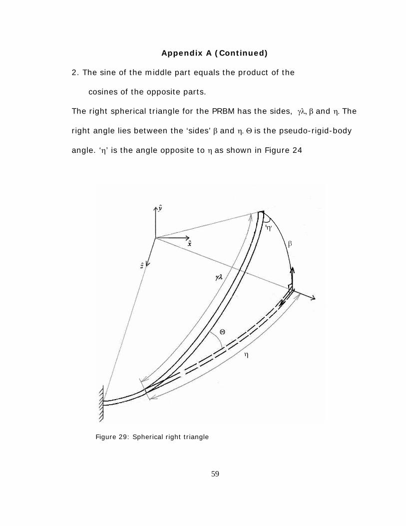
The right spherical triangle for the PRBM has the sides, γλ, β and η. The

right angle lies between the ‘sides’ β and η. Θ is the pseudo-rigid-body

angle. ‘η’ is the angle opposite to η as shown in Figure 24

Figure 29: Spherical right triangle

60


Figure 30: Five parts for PRBM right spherical triangle.

Using Napier Rules the following equations can be obtained.

)90tan(tan)90sin( Θ−=Θ− η

Where )()( γλλφλη −−−=

and φλα −=

To get

⎥⎦

⎤⎢⎣

⎡−−

=Θ −

)]1(sin[tantan 1

γλαβ

61


At β=90o this equation fails to give a value of pseudo-rigid body

angle, Θ, to overcome this, Θ is also expressed in an alternate form.

From Napier Rules we get

γλβ

sinsinsin =Θ

and

γλη cottancos =Θ

To get

⎥⎥⎥

⎦

⎤

⎢⎢⎢

⎣

⎡=Θ −

γληγλ

β

cottansin

sintan 1

62

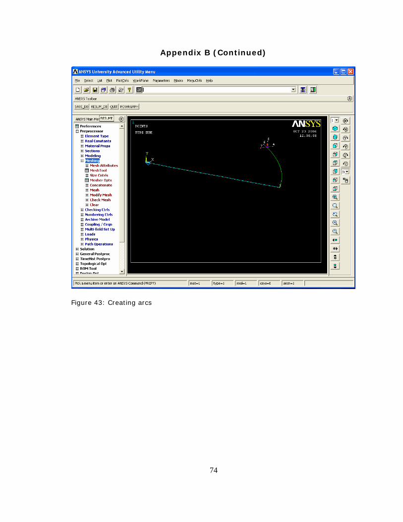
Appendix B Manual for FEA

The following figures (31-54) show a step by step process to run

a single simulation for a single load step.

Figure 31: Activating Graphical User Interface (GUI)

63

Appendix B (Continued)

Figure 32: Limiting the GUI options to structural preferences

64


Figure 33: Adding or defining new element types

65


Figure 34: Beam elements

66


Figure 35: Defining real constants for respective elements

67


Figure 36: Inputting area and moment of inertia values to elements

68


Figure 37: Defining material properties

69


Figure 38: Creating key-points on work-plane through GUI

70


Figure 39: Creating key-points using command line

71


Figure 40: Pan, zoom, rotate

72


Figure 41: Defining of orthogonal triad at beam end

73


Figure 42: Creating lines

74


Figure 43: Creating arcs

75


Figure 44: Meshing

76


Figure 45: Mesh attributes for line

77


Figure 46: Allocating specific material to mesh (elements)

78


Figure 47: Selecting analysis type

79


Figure 48: Large displacement analysis selected

80


Figure 49: Equation chosen solvers

81


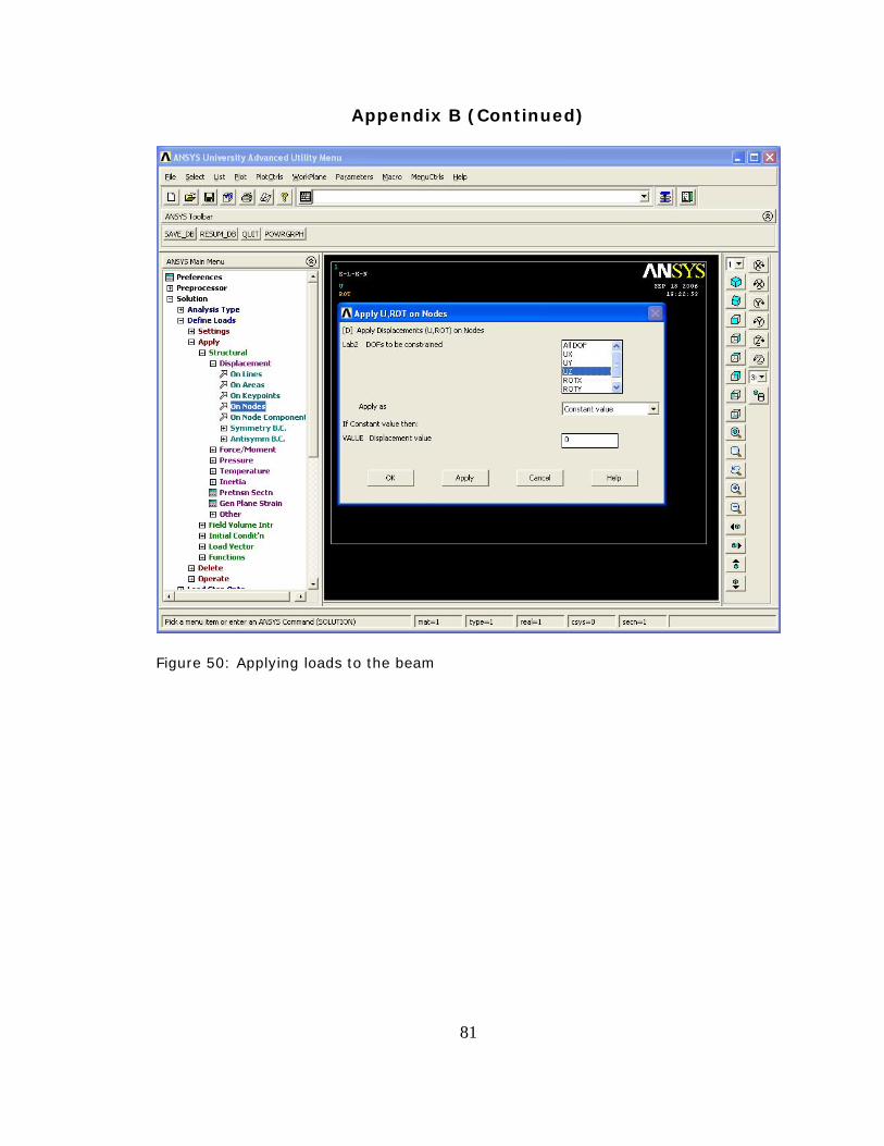
Figure 50: Applying loads to the beam

82


Figure 51: Solve

83


Figure 52: During solve

84


Figure 53: Output

85


Figure 54: To get the log-file

A log file is obtained and is modified to solve for 200 load steps

at a given aspect ratio and arc-length as follows:

!************************************

/CONFIG,NRES,10000

/CWD,'C:\Documents and

Settings\sjagirda\Directory200steps\arc90_asp0.1'

/NOPR

/PMETH,OFF,0

86


KEYW,PR_SET,1

KEYW,PR_STRUC,1

/GO

!************************************

/PREP7

R=1000

PI=acos(-1.)

!************************************

A1=2500.0

Iy1=520833.333

Iz1=520833.333

E1=300000

!************************************

A2= 250.0000037252903

Iy2= 520.8333566163981

Iz2= 52083.33410943548

E2= 300

!************************************

ET,1,BEAM4

!*

ET,2,BEAM4

87


!*

R,1,A1,Iy1,Iz1, , , ,

RMORE, , , , , , ,

!*

R,2,A2,Iy2,Iz2, , , ,

RMORE, , , , , , ,

!*

!*

MPTEMP,,,,,,,,

MPTEMP,1,0

MPDATA,EX,1,,E1

MPDATA,PRXY,1,,0.35

MPTEMP,,,,,,,,

MPTEMP,1,0

MPDATA,EX,2,,E2

MPDATA,PRXY,2,,0.35

!************************************

K,1,0,0,0,

!************************************

arclength=90

xcoor=R*cos(arclength*PI/180)

88


zcoor=R*sin(arclength*PI/180)

K,2,xcoor,0,zcoor,

!************************************

K,3,1000,0,0,

K,4,1050,0,0,

K,5,1000,50,0,

K,6,1000,0,-50,

/USER, 1

/FOC, 1, 538.256940599 , -110.688686131 , 475.000000000

/REPLO

/VIEW, 1, -0.246365419055 , 0.245754775350 ,

0.937501291032

/ANG, 1, -1.91248212175

/REPLO

/VIEW, 1, -0.378438950955 , 0.367160066605 ,

0.849692559630

/ANG, 1, -4.76219842328

/REPLO

K,7,950,0,0,

/FOC, 1, 427.888273403 , -68.9410891494 , 407.804103704

/REPLO

89


/FOC, 1, 456.194825599 , -81.6519820718 , 425.903867008

/REPLO

/VIEW, 1, -0.455467710156 , 0.439135756168 ,

0.774408776203

/ANG, 1, -7.33131293670

/REPLO

LSTR, 1, 2

LSTR, 3, 4

LSTR, 3, 5

LSTR, 3, 6

LSTR, 3, 7

!*

LARC,2,3,1,1000,

FLST,5,5,4,ORDE,2

FITEM,5,1

FITEM,5,-5

CM,_Y,LINE

LSEL, , , ,P51X

CM,_Y1,LINE

CMSEL,S,_Y

!*

90


!*

CMSEL,S,_Y1

LATT,1,1,1, , , ,

CMSEL,S,_Y

CMDELE,_Y

CMDELE,_Y1

!*

FLST,5,1,4,ORDE,1

FITEM,5,1

CM,_Y,LINE

LSEL, , , ,P51X

CM,_Y1,LINE

CMSEL,,_Y

!*

LESIZE,_Y1, , ,10, , , , ,1

!*

FLST,5,4,4,ORDE,2

FITEM,5,2

FITEM,5,-5

CM,_Y,LINE

LSEL, , , ,P51X

91


CM,_Y1,LINE

CMSEL,,_Y

!*

LESIZE,_Y1, , ,1, , , , ,1

!*

FLST,2,5,4,ORDE,2

FITEM,2,1

FITEM,2,-5

LMESH,P51X

GPLOT

CM,_Y,LINE

LSEL, , , , 6

CM,_Y1,LINE

CMSEL,S,_Y

!*

!*

CMSEL,S,_Y1

LATT,2,2,2, , , ,

CMSEL,S,_Y

CMDELE,_Y

CMDELE,_Y1

92


!*

FLST,5,1,4,ORDE,1

FITEM,5,6

CM,_Y,LINE

LSEL, , , ,P51X

CM,_Y1,LINE

CMSEL,,_Y

!*

LESIZE,_Y1, , ,100, , , , ,1

!*

LMESH, 6

FINISH

/SOL

ANTYPE,0

NLGEOM,1

NSUBST,10,0,0

OUTRES,ERASE

OUTRES,NSOL,-10

RESCONTRL,DEFINE,ALL,-10,1

FLST,2,1,1,ORDE,1

FITEM,2,1

93


!*

!************************************

/GO

D,1, ,0, , , ,UX,UY,UZ,ROTX,ROTZ,

FLST,2,1,1,ORDE,1

FITEM,2,2

!*

/GO

D,2, ,0, , , ,UY, , , , ,

FLST,2,1,1,ORDE,1

FITEM,2,12

!*

!************************************

/GO

!************************************

loadsteps=200

*DO,step,1,loadsteps,1

theta=step*arclength/200

/GO

DDELE,12,ALL

!************************************

94


D,12, ,0, , , ,UZ, , , , ,

FLST,2,1,1,ORDE,1

FITEM,2,12

dispx=-(R-(R*cos(theta*PI/180)))

dispy=R*sin(theta*PI/180)

D,12, ,dispx, , , ,UX, , , , ,

FLST,2,1,1,ORDE,1

FITEM,2,12

!*

/GO

D,12, ,dispy, , , ,UY, , , , ,

FLST,2,1,1,ORDE,1

FITEM,2,12

!*

/GO

D,12, ,theta*PI/180, , , ,ROTZ, , , , ,

LSWRITE,step

*ENDDO

LSSOLVE,1,loadsteps

95


/STATUS,SOLU

FINISH

!************************************

SAVE,'arc90_asp0.1','db','C:\DOCUME~1\SJAGIRDA\Directory200steps

\arc90_asp0.1'

!************************************

*do,i,1,200,1,

/POST1

/OUTPUT,arc90_asp0.1,txt,,APPEND

SET,,,,,i,,,

FLST,5,6,1,ORDE,4

FITEM,5,1

FITEM,5,-2

FITEM,5,12

FITEM,5,-15

NSEL,S, , ,P51X

PRNSOL,DOF,

/OUT

*ENDDO

*do,i,1,200,1,

/POST1

96


/OUTPUT,arc90_asp0.1,m,,APPEND

SET,,,,,i,,,

FLST,5,6,1,ORDE,4

FITEM,5,1

FITEM,5,-2

FITEM,5,12

FITEM,5,-15

NSEL,S, , ,P51X

PRNSOL,DOF,

/OUT

*ENDDO

*do,i,1,200,1,

/POST1

/OUTPUT,arc90_asp0.1BETA,txt,,APPEND

SET,,,,,i,,,

FLST,5,6,1,ORDE,4

NSEL,S, , ,12

PRNSOL,ROT,Z

/OUT

*ENDDO

*do,i,1,200,1,

97


/POST1

/OUTPUT,arc90_asp0.1DISPX,txt,,APPEND

SET,,,,,i,,,

FLST,5,4,1,ORDE,2

FITEM,5,12

FITEM,5,-15

NSEL,S, , ,P51X

PRNSOL,U,X

/OUT

*ENDDO

*do,i,1,200,1,

/POST1

/OUTPUT,arc90_asp0.1DISPY,txt,,APPEND

SET,,,,,i,,,

FLST,5,4,1,ORDE,2

FITEM,5,12

FITEM,5,-15

NSEL,S, , ,P51X

PRNSOL,U,Y

/OUT

*ENDDO

98


*do,i,1,200,1,

/POST1

/OUTPUT,arc90_asp0.1DISPZ,txt,,APPEND

SET,,,,,i,,,

FLST,5,4,1,ORDE,2

FITEM,5,12

FITEM,5,-15

NSEL,S, , ,P51X

PRNSOL,U,Z

/OUT

*ENDDO

*do,i,1,200,1,

/POST1

/OUTPUT,arc90_asp0.1PHI,txt,,APPEND

SET,,,,,i,,,

NSEL,S, , ,2

PRNSOL,ROT,Y

/OUT

*ENDDO

FINISH

/EOF

99


The respective parameters affected by change in aspect ratio like real

constants are then changed in this log file and run separately to obtain

respective outputs. The outputs are also limited to the Nodes of

interest.

100

Appendix C Algorithms to Find γ

Algorithm to find γ for load-steps at every one degree

MATLAB Program is as follows.

clear all

start=16;

finish=112;

for arclength=start:2:finish

counter=(arclength+2-start)/2;

for aspect=0.1:0.1:1

countas=round(10*aspect);

%Input

str1 = [];

if round(aspect)==aspect,

str1='.0';

end

string =

['\arc',num2str(arclength),'_asp',num2str(aspect),str1,'ex.txt'];

101

Appendix C (Continued)

fid = fopen(['C:\Documents and

Settings\sjagirda\output\arc',num2str(arclength),string]);

A = fread(fid);

fclose(fid);

G = native2unicode(A)';

s_i = findstr('ROTZ', G);

s_f = findstr('MAXIMUM', G);

cr = native2unicode(10);

space = native2unicode(9);

for j = 1:length(s_i)

M = strtrim(G(s_i(j)+4:s_f(j)-1));

M = strrep(M, cr, space);

M = str2num(M);

beta(j) =M(3,7);

PHI(j) =M(2,6);

B = [ cos(beta(j)) sin(beta(j)) 0 ; -sin(beta(j))

cos(beta(j)) 0 ; 0 0 1 ];

newcs = [ 50 0 0 ; 0 50 0 ; 0 0 -50 ];

dispatbeta=[ M(3,2) M(3,3) M(3,4) ;

M(4,2) M(4,3) M(4,4) ;

102


M(5,2) M(5,3) M(5,4) ;

M(6,2) M(6,3) M(6,4) ];

orgcoord = [ 1000 0 0; 1050 0 0; 1000 50 0;

1000 0 -50];

Finalcoord=dispatbeta+orgcoord;

node12=[

Finalcoord(1,1:3);Finalcoord(1,1:3);Finalcoord(1,1:3);Finalcoord(1,1:

3)];

position_vectorbeta=Finalcoord - node12;

position_vectorbeta(1,:) = [];

A = B*newcs*inv(position_vectorbeta);

thetaobeta(j)=acos(A(2,2));

end

%plot(PHI)

beta(j) =M(3,7);

PHI(j) =M(2,6);

lambda=arclength*pi/180;

BG=zeros(arclength,151);

103


Beta=0;

for countk=1:1:301

for countBETA=1:1:arclength

oldbeta=Beta;

newbeta=beta(1,countBETA);

if newbeta==oldbeta

countBETA=countBETA-1;

break;

else

Beta=newbeta;

gamma=(countk/2000+.7495);

gamma_l = gamma*lambda;

phi=PHI(1,countBETA);

captheta = atan(tan(Beta)./sin((lambda-phi)-

(lambda-gamma_l)));

abs_epsilon_e = sqrt((cos(Beta).*cos(phi)-

ones(size(Beta))).^2+(sin(Beta)).^2.*(cos(phi)).^2+(sin(phi)).^2);

epsilon_ex = cos(Beta).*cos(phi)-1;

epsilon_ey = sin(Beta);

epsilon_ez = cos(Beta).*sin(phi);

104


epsilon_ax = (cos(gamma_l)).^2.*(1-

cos(captheta))+cos(captheta)-1;

epsilon_ay = sin(captheta).*sin(gamma_l);

epsilon_az = sin(gamma_l).*cos(gamma_l).*(1-

cos(captheta));

error = sqrt((epsilon_ex-epsilon_ax).^2

+(epsilon_ey-epsilon_ay).^2 +(epsilon_ez-epsilon_az).^2);

rel_error = error./abs_epsilon_e;

captheta1(countBETA,countk)=captheta;

abs_epsilon_e1(countBETA,countk) =

abs_epsilon_e;

epsilon_ex1(countBETA,countk) = epsilon_ex;

epsilon_ey1(countBETA,countk) = epsilon_ey;

epsilon_ez1(countBETA,countk) = epsilon_ez;

epsilon_ax1(countBETA,countk) = epsilon_ax;

epsilon_ay1(countBETA,countk) = epsilon_ay;

epsilon_az1(countBETA,countk) = epsilon_az;

error1(countBETA,countk)=error;

rel_error1(countBETA,countk)=rel_error;

if rel_error <= 0.005

105




BG(countBETA,countk)=countBETA*countk;

betamax(countk) = Beta;

maxfortheta(countk,countBETA)=Beta;

else

break

end

end

end

end

[y,i] = max(betamax);

gammastar = (i/2000+.7495);

gammastar_l=lambda*gammastar;

[p,q]=max(maxfortheta);

[r,s]=max(q);

Beta=beta(1,s);

phi=PHI(1,s);

thetaostar=thetaobeta(1,s);

106


capthetastar =atan(tan(Beta)./sin((lambda-phi)-(lambda-

gammastar_l)));

CTHETAstar=capthetastar/thetaostar;

GAMMA_MATRIX(counter,countas)=gammastar;

CAPTHETA_MATRIX(counter,countas)=capthetastar;

CTHETA_MATRIX(counter,countas)=CTHETAstar;

end

end

GAMMA_MATRIX;

CTHETA_MATRIX;

CAPTHETA_MATRIX;

figure(1)

plot(GAMMA_MATRIX)

figure(2)

plot(CTHETA_MATRIX)

figure(3)

plot(CAPTHETA_MATRIX)

107


Algorithm to find γ for 200 load-steps.

clear all

start=4;

finish=112;

for arclength=start:2:finish

arclength

counter=(arclength+2-start)/2;

asp=[0.1 0.4 0.7];

for i=1:3

aspect=asp(i);

aspect;

countas=round(10*aspect);

%Input

str1 = [];

if round(aspect)==aspect,

str1='.0';

end

string =

['arc',num2str(arclength),'_asp',num2str(aspect),str1];

108


fid1 = fopen(['C:\Documents and

Settings\sjagirda\Directory200steps\',string,'\',string,'BETA.txt']);

ABT = fread(fid1);

fclose(fid1);

GBT = native2unicode(ABT)';

s_iB = findstr('ROTZ', GBT);

s_fB = findstr('MAXIMUM', GBT);



for j = 1:length(s_iB)

BT = strtrim(GBT(s_iB(j)+4:s_fB(j)-1));

BT = strrep(BT, cr, space);

BT = str2num(BT);

beta(j) =BT(1,2);

end

string =

['arc',num2str(arclength),'_asp',num2str(aspect),str1];


Settings\sjagirda\Directory200steps\',string,'\',string,'PHI.txt']);

APH = fread(fid2);

109


fclose(fid2);

GPH = native2unicode(APH)';

s_iP = findstr('ROTY', GPH);

s_fP = findstr('MAXIMUM', GPH);



for j = 1:length(s_iP)

PH = strtrim(GPH(s_iP(j)+4:s_fP(j)-1));

PH = strrep(PH, cr, space);

PH = str2num(PH);

PHI(j) =PH(1,2);

end

PHI(j);


Settings\sjagirda\Directory200steps\',string,'\',string,'DISPX.txt']);

DISPXA = fread(fid3);

fclose(fid3);

DISPXG = native2unicode(DISPXA)';

s_iX = findstr('UX', DISPXG);

s_fX = findstr('MAXIMUM', DISPXG);

110



Settings\sjagirda\Directory200steps\',string,'\',string,'DISPY.txt']);

DISPYA = fread(fid4);

fclose(fid4);

DISPYG = native2unicode(DISPYA)';

s_iY = findstr('UY', DISPYG);

s_fY = findstr('MAXIMUM', DISPYG);


Settings\sjagirda\Directory200steps\',string,'\',string,'DISPZ.txt']);

DISPZA = fread(fid5);

fclose(fid5);

DISPZG = native2unicode(DISPZA)';

s_iZ = findstr('UZ', DISPZG);

s_fZ = findstr('MAXIMUM', DISPZG);



for j = 1:length(s_iX)

111


M = strtrim(DISPXG(s_iX(j)+4:s_fX(j)-1));

M = strrep(M, cr, space);

M = str2num(M);

NODE12DISPX =M(1,2);




N = strtrim(DISPYG(s_iY(j)+4:s_fY(j)-1));

N = strrep(N, cr, space);

N = str2num(N);

NODE12DISPY =N(1,2);




O = strtrim(DISPZG(s_iZ(j)+4:s_fZ(j)-1));

O = strrep(O, cr, space);

O = str2num(O);

NODE12DISPZ =O(1,2);


112




B = [ cos(beta(j)) sin(beta(j)) 0 ; -sin(beta(j))

cos(beta(j)) 0 ; 0 0 1 ];

newcs = [ 50 0 0 ; 0 50 0 ; 0 0 -50 ];

dispatbeta=[ NODE12DISPX NODE12DISPY

NODE12DISPZ ;

NODE13DISPX NODE13DISPY

NODE13DISPZ ;


NODE14DISPZ ;


NODE15DISPZ ];

orgcoord = [ 1000 0 0; 1050 0 0; 1000 50 0;

1000 0 -50];

Finalcoord=dispatbeta+orgcoord;

node12=[

Finalcoord(1,1:3);Finalcoord(1,1:3);Finalcoord(1,1:3);Finalcoord(1,1:

3)];

position_vectorbeta=Finalcoord - node12;

113


position_vectorbeta(1,:) = [];

A = B*newcs*inv(position_vectorbeta);

thetaobeta(j)=acos(A(2,2));

end

lambda=arclength*pi/180;

BG=zeros(arclength,151);

Beta=0;

for countk=1:1:501

for countBETA=1:1:200

oldbeta=Beta;

newbeta=beta(1,countBETA);

if newbeta==oldbeta

countBETA=countBETA-1;

break;

else

Beta=newbeta;

gamma=(countk/2000+.7495);

gamma_l = gamma*lambda;

phi=PHI(1,countBETA);

114


sincaptheta=sin(Beta)./sin(gamma_l);

coscaptheta=tan((lambda-phi)-(lambda-

gamma_l)).*cot(gamma_l);

% captheta = atan(tan(Beta)./sin((lambda-phi)-

(lambda-gamma_l)));

captheta = atan2(sincaptheta,coscaptheta);

abs_epsilon_e = sqrt((cos(Beta).*cos(phi)-

ones(size(Beta))).^2+(sin(Beta)).^2.*(cos(phi)).^2+(sin(phi)).^2);

epsilon_ex = cos(Beta).*cos(phi)-1;

epsilon_ey = sin(Beta);

epsilon_ez = cos(Beta).*sin(phi);

epsilon_ax = (cos(gamma_l)).^2.*(1-

cos(captheta))+cos(captheta)-1;

epsilon_ay = sin(captheta).*sin(gamma_l);

epsilon_az = sin(gamma_l).*cos(gamma_l).*(1-

cos(captheta));

error = sqrt((epsilon_ex-epsilon_ax).^2

+(epsilon_ey-epsilon_ay).^2 +(epsilon_ez-epsilon_az).^2);

rel_error = error./abs_epsilon_e;

115


captheta1(countBETA,countk)=captheta;

abs_epsilon_e1(countBETA,countk) =

abs_epsilon_e;

epsilon_ex1(countBETA,countk) = epsilon_ex;

epsilon_ey1(countBETA,countk) = epsilon_ey;

epsilon_ez1(countBETA,countk) = epsilon_ez;

epsilon_ax1(countBETA,countk) = epsilon_ax;

epsilon_ay1(countBETA,countk) = epsilon_ay;

epsilon_az1(countBETA,countk) = epsilon_az;



if rel_error <= 0.005



BG(countBETA,countk)=countBETA*countk;

betamax(countk) = Beta;

maxfortheta(countk,countBETA)=Beta;

else

break

end

116


end

end

end

[y,i] = max(betamax);

gammastar = (i/2000+.7495);

gammastar_l=lambda*gammastar;

[p,q]=max(maxfortheta);

[r,s]=max(q);

Beta=beta(1,s);

phi=PHI(1,s);

thetaostar=thetaobeta(1,s);

sincapthetastar=sin(beta)./sin(gammastar_l);

coscapthetastar=tan((lambda-PHI)-(lambda-

gammastar_l)).*cot(gammastar_l);

capthetastar = atan2(sincapthetastar,coscapthetastar);

% capthetastar =atan2(tan(beta),sin((lambda-PHI)-

(lambda-gammastar_l)));

[p2,s2] = polyfit(capthetastar(1:s),thetaobeta(1:s),1);

117


CTHETAstar=p2(1);

GAMMA_MATRIX(counter,countas)=gammastar;

CAPTHETA_MATRIX(counter,countas)=capthetastar(s)*(180/pi);

CTHETA_MATRIX(counter,countas)=CTHETAstar;

end

%plot([0.1:.1:1],GAMMA_MATRIX(arclength,:));

%drawnow

end

GAMMA_MATRIX;

CTHETA_MATRIX;

CAPTHETA_MATRIX;

figure(1)

plot([4:2:112],GAMMA_MATRIX)

xlabel('arc length , \lambda (degrees)')

ylabel('Characteristic radius factor, \gamma')

figure(2)

plot([4:2:112],CTHETA_MATRIX)

xlabel('arc length, \lambda (degrees)')

118


ylabel('Parametric angle coefficient, C_\Theta')

figure(3)

plot([4:2:112],CAPTHETA_MATRIX)

xlabel('arc length, \lambda (degrees)')

ylabel('Parameterization limit, \Theta_{max} (degrees) for the

parametric angle coefficient, C_\Theta_{max}')

119

Appendix D Summary

Table 1: Spherical PRBM

)cos(tantan)1( 1 Θ+−= − γλλγα

)sin(sinsin 1 Θ= − γλβ

θ0=Cθ Θ

])]()sin[(

tan[tan 1

γλλφλβ

−−−=Θ −

2/1222 }]sin[cossin]1cos{[cos φββφβε ++−=e

2/1222 })]cos1(cos[sin]sin[sin]cos)cos1({[cos Θ−+Θ+Θ+Θ−= γλγλγλγλε a

2/12

22

})]cos1(cossinsin[cos]sinsin[sin)]1cos)cos1((cos)1cos{[(cos

Θ−−

Θ−+−Θ+Θ−−−=

γλγλφβ

γλβγλφβerror

2/1222

2/12

22

}]sin[cossin]1cos{[cos})]cos1(cossinsin[cos

]sinsin[sin)]1cos)cos1((cos)1cos{[(cos

φββφβγλγλφβ

γλβγλφβ

ε ++−Θ−−

Θ−+−Θ+Θ−−−

=e

error

For small angles when the sphere has a very large radius the above

formulas can be approximated to the planar case.

120

Appendix D (Continued)

Table 2: Planar PRBM

))cos1(1( Θ−−= γla

Θ= sinlb γ

θ0=Cθ Θ

)1(tan 1

γ−−=Θ −

lab

22)( bale +−=δ

22 )sin()]cos1([ Θ+Θ−= lla γγδ

22 ]sin)/[()]}cos1(1[)/{( Θ−+Θ−−−= γγ lblaerror

22

22

)/()/1(

]sin)/[()]}cos1(1[)/{(

lbla

lblaerror

e +−

Θ−+Θ−−−=

γγε

Kinematics of curved flexible beam

Documents

Transcript of Kinematics of curved flexible beam