Key words Navier-Stokes equation, Aeroacoustic, Litghill’s ...
46
Abstract In this work a stabilized formulation of the finite element method for solving the incom- pressible Navier-Stokes equation and Lighthill’s tensor for calculation of acoustic sources are presented. The important feature of this formulation resides in the design of the stabilization terms, which serve several purposes. First, convective dominated flows in the Navier-Stokes equation can be dealt with. Second, there is no need to use interpolation spaces subject to an inf-sup condition for the velocity-pressure pair and therefore linear interpolation spaces can be used. Finally, this formulation allows a more accurate computation of Lighthill’ tensor and a better representation of acoustics sources. Key words : Navier-Stokes equation, Aeroacoustic, Litghill’s tensor, stabilized finite element, variational multiscale method, monolithic scheme. 1
Transcript of Key words Navier-Stokes equation, Aeroacoustic, Litghill’s ...

Abstract
In this work a stabilized formulation of the finite element method for solving the incom-pressible Navier-Stokes equation and Lighthill’s tensor for calculation of acoustic sources arepresented. The important feature of this formulation resides in the design of the stabilizationterms, which serve several purposes. First, convective dominated flows in the Navier-Stokesequation can be dealt with. Second, there is no need to use interpolation spaces subject toan inf-sup condition for the velocity-pressure pair and therefore linear interpolation spacescan be used. Finally, this formulation allows a more accurate computation of Lighthill’tensor and a better representation of acoustics sources.
Key words : Navier-Stokes equation, Aeroacoustic, Litghill’s tensor, stabilized finite element,variational multiscale method, monolithic scheme.
1

Contents
1 Introduction and objectives 4
2 Proposed methodology to solve aeroacoustics sources 52.1 First step: Computational Fluid Dynamics Simulation . . . . . . . . . . . . . . 52.2 Second step: The source term . . . . . . . . . . . . . . . . . . . . . . . . . . . . 6
3 Problem statement 63.1 Weak form of the Navier Stokes equation . . . . . . . . . . . . . . . . . . . . . 63.2 Time discretisation and linearization of the Navier-Stokes equations . . . . . . 7
3.2.1 First order schemes . . . . . . . . . . . . . . . . . . . . . . . . . . . . . . 73.2.2 Second order schemes . . . . . . . . . . . . . . . . . . . . . . . . . . . . 8
3.3 Galerkin finite element approximation of the Navier-Stokes equations . . . . . . 8
4 LES: Large Eddy simulation 84.1 Filtered Navier-Stokes equation . . . . . . . . . . . . . . . . . . . . . . . . . . . 94.2 Some drawbacks of LES . . . . . . . . . . . . . . . . . . . . . . . . . . . . . . . 10
5 Subgrid Scale (SGS) stabilised finite element methods 105.1 Outline of the SGS stabilisation approach . . . . . . . . . . . . . . . . . . . . . 105.2 SGS with quasi static and dynamical subscales stabilised finite element method
for the Navier-Stokes equations . . . . . . . . . . . . . . . . . . . . . . . . . . . 115.3 Some physical properties of the formulation . . . . . . . . . . . . . . . . . . . . 14
5.3.1 Conservation of momentum . . . . . . . . . . . . . . . . . . . . . . . . . 145.3.2 A door to turbulence . . . . . . . . . . . . . . . . . . . . . . . . . . . . . 15
6 Dissipative structure and backscatters 166.1 Energy balance equation for the Navier stokes problem . . . . . . . . . . . . . . 166.2 Energy balance equation for a Large Eddy Simulation model . . . . . . . . . . 176.3 Energy balance for the orthogonal subgrid scale with quasi-static and dynamical
subscales finite element approach to the Navier-Stokes problem . . . . . . . . . 186.4 Local kinetic energy balance equations . . . . . . . . . . . . . . . . . . . . . . . 206.5 Backscatters . . . . . . . . . . . . . . . . . . . . . . . . . . . . . . . . . . . . . . 21
7 Fourier Transform 227.1 Discrete Fourier Transform . . . . . . . . . . . . . . . . . . . . . . . . . . . . . 22
8 The acoustics sources 23
9 Numerical experimentation 249.1 CFD simulation of generic landing gear struts with horizontal angle α = 0o using
LES model and SGS stabilisation method with dynamical subscales . . . . . . 249.2 CFD simulation of generic landing gear struts with horizontal angle α = 15o
using LES model and SGS stabilisation method with dynamical subscales . . . 329.3 Acoustics sources generated by a single cylinder at Re=500 . . . . . . . . . . . 399.4 Acoustics sources generated by parallel cylinders at Re=1000 . . . . . . . . . . 42
10 Conclusions 45
2

11 Future work 45
3

1 Introduction and objectives
With the constant need to travel faster, better and safer through air the industry of aeronauticsbecame one of industries with the highest progression in the last century. From the first flightof Wright’s brothers until now, men have produced powerfull aircrafts. With these aircraftspeople can travel very fast and safe from one point on earth to another, but like everythingelse, when there is some progress there is the need to pay some costs. One of this costs is thesound generated from aircrafts. In one long period of aviation history, scientists and engineersthought that sound generated from aircraft was only produced in the engine. During the 1960’sand 1970’s Lighthill noticed that flow around aircrafts (aerodynamics) also produce some partof sound. With this discovery a new field emerged, Aeroacoustics. This field has emerged fromthe fields of acoustics and fluid mechanics and is concerned with sound generated by unsteadyand/or turbulent flows and also by their interaction with solid boundaries. This type of soundis comonly known as aerodynamic sound. In contrast to classical acoustics, forces and mo-tions inside the flow are the sources of sound rather than the externally applied ones. On theother hand Computational Aeroacoustics (CAA) is a relatively new computational field thataims at simulatig and predicting aerodynamically generated noise. With constant developingof computers CAA has become nowdays an active research field due to its applications in theaeronautics, railway, automotive and underwater industrie. The objective of this work is topresent a finite element method for the approximation of incompressible Navier-Stokes equa-tion and calculation of Lighthill’s tensor which arise in Aeroacoustics as acoustics sources.These sources are the source for the inhomogeneous Helmholtz equation which calculate pres-sure fields to predict sound in domains. Lighthill showed how the compressible Navier-Stokesequation could be reordered in the form of an inhomogeneous acoustic wave equation witha source term built from the double divergence of what is now known as Lighthill’s tensor.This tensor involves combination of the flow variables and their derivatives (velocity, pressureand density), and under certain hypothes it acquires a simple, treatable expression. This workwill show how different methods of stabilization for the Navier-Stokes equation gives differentsolution of calculation of Lighthill’s tensor. The stabilization technique presented in this workis developed in the variational multiscale framework. It is based on a two-scale decompositionof the unknowns in the finite element component and a subgrid scale or subscale which corre-sponds to the unknown component that cannot be captured by the finite element space. Theidea followed was first presented in [4]. In particular, the version for systems of equations wasintroduced in [2] .The key point is the approximation of the subgrid scales. In this work it hasbeen chosen the simplest approach that consists of taking them proportional to a projectionof the residual of the finite element approximation multiplied by a matrix of stabilization pa-rameters. Among the several options to select the projection and the structure of the matrix ofstabilization parameters, the identity and a diagonal structure have been chosen, respectively.Up to this point, the only missing issue to close the formulation is the design of the stabilizationparameters. It has been done based on the stability and convergence analysis of the method.
The usual approach for solving the Navier-Stokes equations like a part of the Aeroacousticproblem is to use LES (Large Eddy simulation) to simulate turbulent flows which arise in highReynolds numbers. LES performs a spatial scale decomposition equations for the velocity andpressure. (u, p) stands for large scales that are expected to be computationally resolvable, while(u
′, p
′), stands for the small scales, which are not expected to be captured. The goal of this
work is to show how these small scales can be modelled and how these small scales afect thesimulation of turbulent flow problems.
The paper is organized as follows. In Section 2 methodology for solving aeroacoustics sources
4

of sound is proposed. In Section 3 the first step problem (Computational Fluid Dynamics) isstated both in its continuous and its variational form. Issues regarding the time integrationand the linearization of the non-linear term are discussed in this section, leading to a timediscrete and linearized scheme. After that there is a short presentation of Large Eddy simulation(LES) in Section 4. Next, the subgrid scale framework is explained in section 5 for quasi-static and dynamical subscales. After proposing the stabilization method, there is a discussionenergy balance for Navier-Stokes equation using LES and SGS approach in Section 6. Shortintroduction to Fourier transform is presented in Section 7. Way how to calculate Litghill’stensor is presented in Section 8. Numerical experiments verifying the theoretical results areexplained in Section 9 and finally some conclusions are drawn in Section 10 and future workin Section 11.
2 Proposed methodology to solve aeroacoustics sources
2.1 First step: Computational Fluid Dynamics Simulation
The CFD(Computational Fluid Dynamics) computation aims at obtaining the flow velocityvector u, from the solution of the time evolving incompressible Navier-Stokes equation. Themathematical problem consists in solving the latter equation in a given computational domainΩ ⊂ Rd (where d=2 or 3 is the number of space dimensions) with boundary Γ = ∂Ω andprescribed initial and boundary conditions. The boundary Γ = ∂Ω can be split into two disjointsets (∂Ω = ΓD ∪ ΓN ) respectively accounting for those boundaries with prescribed Dirichletand Neumann conditions. The problem can be derived as:
∂tu+ u · ∇u− ν∆u+∇p = f in Ω, t > 0, (1)
∇ · u = 0, in Ω, t > 0 (2)
u(x, 0) = u0(x) in Ω, t = 0, (3)
u(x, t) = uD(x, t) on ΓD, t > 0, (4)
n · σ(x, t) = tN (x, t) on ΓN , t > 0, (5)
with ν representing the kinematic flow viscosity, f the external force and tN the reaction onthe boundary.In the case of high Reynolds number problems we will be faced with the difficulty to simulateturbulent flows. There exist mainly three options to do so [9], namely the RANS (ReynoldsAvereged Navier-Stokes equation) approach and the DNS ( Direct Numerical solution approachand the LES (Large Eddy Simulation) approach. In general, the RANS approach turns to be notappropriate for aeroacoustic simulation because it cannot properly capture time fluctuations.On the other hand, DNS computational cost scales Re9/4, which makes it not feasible for typicalhigh Reynolds number problems found in aeronautics, railway, or automotive application. Hencethe right option seems to be LES, that performs a spatial decomposition u = u+u
′, p = p+p
′
for the velocity and the pressure in (1) − (5). (u, p) stands for some large scales that areexpected to be computationally resolvable while (u
′, p
′) stands for the small scales, which are
not expected to be computable.In the standard LES approach, the scale decomposition is carried out by convolving (1)− (5)with a filter function. As it is known, this gives place to a closure problem because an extraterm of the type R = u⊗ u− u⊗ u, which has to be modeled, appears in the equation . Thisterm is known as the residual stress tensor. Once having a model for R, the resulting LESequations can be discretised and a numerical solution attempted. However, there is another
5
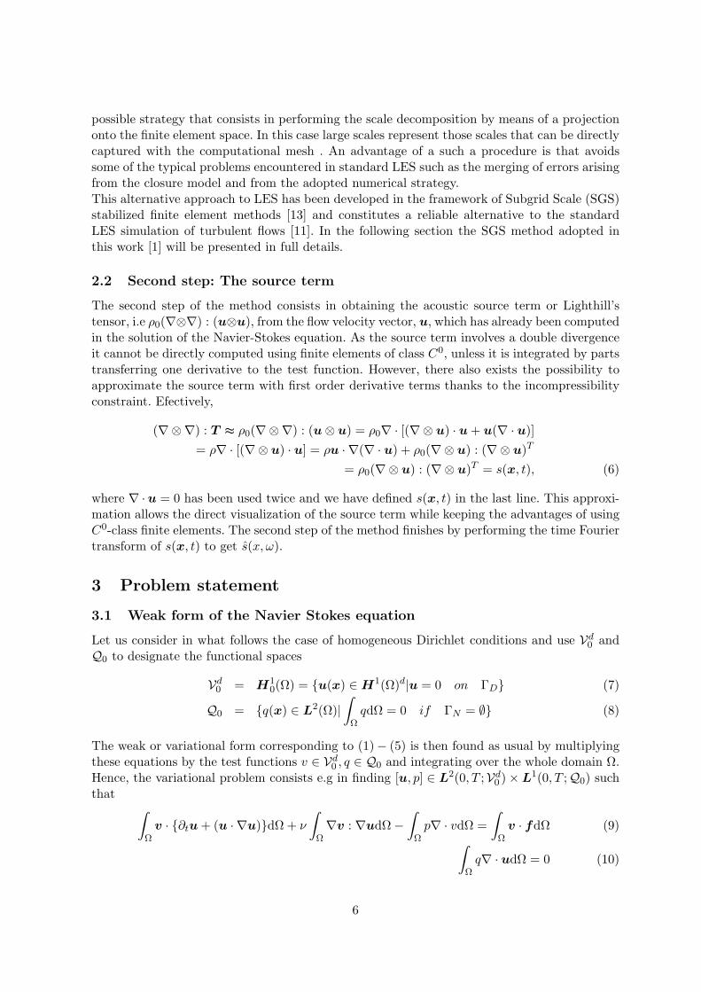
possible strategy that consists in performing the scale decomposition by means of a projectiononto the finite element space. In this case large scales represent those scales that can be directlycaptured with the computational mesh . An advantage of a such a procedure is that avoidssome of the typical problems encountered in standard LES such as the merging of errors arisingfrom the closure model and from the adopted numerical strategy.This alternative approach to LES has been developed in the framework of Subgrid Scale (SGS)stabilized finite element methods [13] and constitutes a reliable alternative to the standardLES simulation of turbulent flows [11]. In the following section the SGS method adopted inthis work [1] will be presented in full details.
2.2 Second step: The source term
The second step of the method consists in obtaining the acoustic source term or Lighthill’stensor, i.e ρ0(∇⊗∇) : (u⊗u), from the flow velocity vector, u, which has already been computedin the solution of the Navier-Stokes equation. As the source term involves a double divergenceit cannot be directly computed using finite elements of class C0, unless it is integrated by partstransferring one derivative to the test function. However, there also exists the possibility toapproximate the source term with first order derivative terms thanks to the incompressibilityconstraint. Efectively,
(∇⊗∇) : T ≈ ρ0(∇⊗∇) : (u⊗ u) = ρ0∇ · [(∇⊗ u) · u+ u(∇ · u)]= ρ∇ · [(∇⊗ u) · u] = ρu · ∇(∇ · u) + ρ0(∇⊗ u) : (∇⊗ u)T
= ρ0(∇⊗ u) : (∇⊗ u)T = s(x, t), (6)
where ∇ ·u = 0 has been used twice and we have defined s(x, t) in the last line. This approxi-mation allows the direct visualization of the source term while keeping the advantages of usingC0-class finite elements. The second step of the method finishes by performing the time Fouriertransform of s(x, t) to get s(x, ω).
3 Problem statement
3.1 Weak form of the Navier Stokes equation
Let us consider in what follows the case of homogeneous Dirichlet conditions and use Vd0 and
Q0 to designate the functional spaces
Vd0 = H1
0(Ω) = u(x) ∈ H1(Ω)d|u = 0 on ΓD (7)
Q0 = q(x) ∈ L2(Ω)|∫ΩqdΩ = 0 if ΓN = ∅ (8)
The weak or variational form corresponding to (1)− (5) is then found as usual by multiplyingthese equations by the test functions v ∈ Vd
0 , q ∈ Q0 and integrating over the whole domain Ω.Hence, the variational problem consists e.g in finding [u, p] ∈ L2(0, T ;Vd
0 )×L1(0, T ;Q0) suchthat ∫
Ωv · ∂tu+ (u · ∇u)dΩ + ν
∫Ω∇v : ∇udΩ−
∫Ωp∇ · vdΩ =
∫Ωv · fdΩ (9)∫
Ωq∇ · udΩ = 0 (10)
6

for all v ∈ Vd0 , q ∈ Q0 . In order to shorten the notation in (9)− (10) and subsequent equations,
we will use
l(v) = 〈v,f〉 (11)
Note that the brackets in (11) corresponds to duality pair between H1/2(ΓN ) andH−1/2(ΓN ) . The weak form can then be rewritten as
(∂tu,v) + 〈u · ∇u,v〉+ ν(∇u,∇v)− (p,∇ · v) = l(v) (12)
(q,∇ · u) = 0 (13)
3.2 Time discretisation and linearization of the Navier-Stokes equations
To find a numerical approximation to the Navier Stokes equations (1) − (5) we will have todiscretise in time and space. The time discretisation scheme that has been used in this work isthe generalized trapezoidal rule. Let us consider a partition of the computational time interval0 < t0 < .... < tN = T with a constant time steps size δt = tn+1 − tn and let us introduce thefollowing notation for a generic time-dependent function ϕ(t)
δϕn = ϕn+1 − ϕn (14)
δϕn+α = αϕn+1 + (1− α)ϕn (15)
δtϕn = δϕn/δt (16)
Where α ∈ [0, 1] and ϕn stands for the value of ϕ at time tn. The time discrete version of theNavier Stokes (1)− (5) for homogeneous Dirichlet conditions can be written as
∂tun +N n(u)− ν∆un+α +∇pn+1 = fn+α in Ω, (17)
∇ · un+α = 0, in Ω, (18)
u0 = u0 in Ω, (19)
un+α = 0 on ΓD, (20)
n · σn+α = tn+αN on ΓN , (21)
with N n(u) representing an approximation to the convective term. Depending on the value ofα in (17) − (21) we will have a first or second order accurate in time scheme for the solution.The most widely used schemes are.
3.2.1 First order schemes
Using α = 0 we will obtain Forward Euler scheme. This scheme is conditionally stable i.e. δthas to be small enough. In this case the convective term is given explicitly N n(u) = (un ·∇)un
Using α = 1 the Backward Euler scheme is obtained. Backward Euler is unconditionally stable.In this case the convection term is given implicitly N n(u) = (un+1 · ∇)un+1. A linearizationprocess is needed at each time step.
7
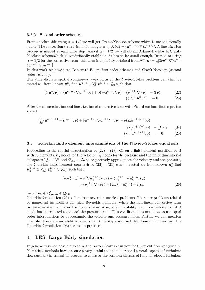
3.2.2 Second order schemes
From another side using α = 1/2 we will get Crank-Nicolson scheme which is unconditionallystable. The convection term is implicit and given by N (u) = (un+1/2 ·∇)un+1/2. A linearizationprocess is needed at each time step. Also if α = 1/2 we will obtain Adams-Bashforth/Crank-Nicolson schemewhich is conditionally stable i.e. δt has to be small enough. Instead of usingα = 1/2 for the convective term, this term is explicitly obtained from N n(u) = 1
2 [3(un ·∇)un−
(un−1 · ∇)un−1]In this work we have used Backward Euler (first order scheme) and Crank-Nicolson (secondorder scheme).The time discrete spatial continuous weak form of the Navier-Stokes problem can then bestated as: from known un, find un+α ∈ Vd
0 , pn+1 ∈ Q0 such that
(δtun,v) + 〈un+α · ∇un+α,v〉+ ν(∇un+α,∇v)− (pn+1,∇ · v) = l(v) (22)
(q,∇ · un+1) = 0 (23)
After time discretisation and linearization of convective term with Picard method, final equationstated
(1
δt(un+1,i+1 − un,i+1,v) + 〈un+1,i · ∇un+1,i+1,v) + ν(4un+1,i+1,v)
−(∇pn+1,i+1,v) = (f ,v) (24)
(∇ · un+1,i+1, q) = 0 (25)
3.3 Galerkin finite element approximation of the Navier-Stokes equations
Proceeding to the spatial discretisation of (22) − (23). Given a finite element partition of Ωwith ne elements, nu nodes for the velocity, np nodes for the pressure and the finite dimensionalsubspaces Vd
h,0 ⊂ Vd0 and Qh,0 ⊂ Q0 to respectively approximate the velocity and the pressure,
the Galerkin finite element approach to (22) − (23) can be stated as: from known unh find
un+αh ∈ Vd
h,0, pn+1h ∈ Qh,0 such that
(δtunh,vh) + ν(∇un+α
h ,∇vh) + 〈un+αh · ∇un+α
h ,vh〉−(pn+1
h ,∇ · vh) + (qh,∇ · un+1h ) = l(vh) (26)
for all vh ∈ Vdh,0, qh ∈ Qh,0
Galerkin formulation (26) suffers from several numerical problems. There are problems relatedto numerical instabilities for high Reynolds numbers, when the non-linear convective termin the equation dominates the viscous term. Also, a compatibility condition (inf-sup or LBBcondition) is required to control the pressure term. This condition does not allow to use equalorder interpolations to approximate the velocity and pressure fields. Further we can mentionthat also there are instabilities when small time steps are used. All these difficulties turn theGalerkin formulation (26) useless in practice.
4 LES: Large Eddy simulation
In general it is not possible to solve the Navier Stokes equation for turbulent flow analytically.Numerical methods have become a very useful tool to understand several aspects of turbulentflow such as the transition process to chaos or the complex physics of fully developed turbulent
8

flow. Numerical methods have become also an indispensable tool to address many engineeringproblems involving turbulence. We have already commented in section 2 that there exist threemain possibilities to perform Computational Fluid Dynamics (CFD) of turbulent flows in thespatial domain [9] namely RANS, DNS and LES methods. It has been argued that the laterturns to be the appropriate approach for the kind of problems we aim to solve and we willconcentrate on it in this section. We remind that the key idea of standard LES is to decomposethe velocity and pressure fields at the continum level, so that [u, p] = [u, p]+ [u
′, p
′] with [u, p]
representing the large scales of the flow that can be computed, whereas [u′, p
′] accounts for the
non-resolvable small scales. The key point in LES consists in properly modeling the effects ofthe non-computable small scales into the large ones
4.1 Filtered Navier-Stokes equation
The scale decomposition between large and small scales has been done traditionally by meansof a filtering process [9]. Without detailing the possible low-pass filter operations and assumingthat the filter (·) : v 7→ v commutes with the differential operators, we can filter the NavierStokes equations (1)− (5) to obtain the system
∂tu+ u · ∇u− ν∆u+∇p = f −∇ · R in Ω× (0, T ) (27)
∇ · u = 0, in Ω× (0, T ) (28)
u = 0 or u periodic on Γ, (29)
u(x, 0) = u0(x) in Ω, (30)
In (27) the tensor R = u⊗ u − u ⊗ u is known as the residual stress tensor, subscale tensoror subgrid scale tensor, In order for (27) − (30) to be a closed system of equations for [u, p]it is need to express R in terms of u. This question is known as closure problem. The variouschoices for R give place to different LES models. Once a model has been chosen, the laststep of LES consists in the discretisation of (27) − (30) and in finding its numerical solution.One could wonder about the possibility of finding an exact closure for (27) − (30) so that Rcould be expressed in terms of u, without making any approximation. This is in fact possibleif we make use of Helmholtz filter that obtains u from the solution of the Helmholtz equationu− ε24u = u. It follows that u = (I − ε24)−1u, with ε > 0 standing for the cut-off scale [3].Taking into account that u⊗ u = (u− ε24u)⊗ (u− ε24u) and applying the filter to u⊗ uwe get u ⊗ u = u⊗ u − ε24u⊗ u. Inserting these relations into the subgrid scale tensor weobtain
Rij = (ui − ε24ui)(uj − ε24uj)− uiuj
= uiuj − ε2uj4ui − ε2ui4uj + ε44ui4uj − uiuj
= ε24(uiuj)− ε2uj4ui − ε2ui4uj + ε44ui4uj
= 2ε2∇ui · ∇uj + ε44ui4uj (31)
The expression effectively allows to write R in terms of u without making any approximation oradding some hypotheses. However, it is to be remarked that the Helmholtz filter establishes anisomorphism between L∞(0, T ;H(Ω)) and L∞(0, T ;H(Ω)∩H2(Ω)), and betwen L2(0, T ;V (Ω))and L2(0, T ;V (Ω) ∩H3(Ω)) . Consequently the exact closure (31) has only served to build anisomorphism between the weak solution of (1) − (5) and the weak solution of (27) − (30) [5].Hence, the number of degrees of freedom needed to solve both problems remains the same. Thisresult can be generalised to any exact closure of equation (27) − (30), so making LES under
9
these circumstances is as much involved as performing DNS. At the first sight this may lookas a paradox fact given that finding an exact closure seems a reasonable goal. However, thisis not the case and LES is only meaningful for a non exact closure so that flow information islost in the subscale modeling.
4.2 Some drawbacks of LES
LES presents several problems and unsolved questions. The key subject still concerns in findinga good model for the subgrid scale tensor. However, it has just been pointed out that achievingan exact closure is a pardox program, so this cannot be a motivation to find subscales models.On the other hand, many of the existing LES models are based on physical and numericalapproximations and heuristic arguments, which perform more or less well depending on theproblem where they are applied. Generalizations are difficut to find although it is recomendedthat the subscales satisfy certain properties such as to conserve the invariance under trans-formations of the original Navier-Stokes equations. However, it is not fully clear which shouldbe characteristic of a good LES model (apart from the obvious fact that it should properlyreproduce experimental data) Another important question concerns the relation/ interactionbetween arising from the physical LES model and from numerical methods used to solve thediscretised problem. It is also not clear which should be the relation between the filter supportε and the characteristic mesh element size h. In addition, the problem of the commutation errorof the filtering and differentiation operations needs also to be addressed. In summary, we couldsay that nowdays a satisfactory mathematical theory of LES still does not exist although stepstowards this direction are being carried out.
5 Subgrid Scale (SGS) stabilised finite element methods
5.1 Outline of the SGS stabilisation approach
In the past two decades, several stabilization strategies have been developed to circumvent thenumerical instabilities that arise in the Galerkin finite element solution of partial differentialequations. We will concentrate here on the Subgrid Scale (SGS) approach (also termed Vari-ational Multiscale Method (VMM) or Residual-Based stabilization) originally developed byHughes [13] for the scalar convection-diffusion-reaction equation and letter extended to otherequations by many authors. for the sake of clarity, the main ideas of the method will be firstoutlined for an abstract stationary variational problem and then explicitly presented in detailfor problems (12) − (13) and in subsequent sections. Let us consider the abstract variationalcontinuous problem of finding y ∈ Y such that
m(y, z) = n(z) (32)
for all z ∈ Z m and n respectively represent (for simplicity) bilinear and linear continuousweak forms, while Y and Z are infinite dimensional spaces. The subgrid scale approach tofind numerical solution to (32) consists in first splitting Y and Z into Y = Yh ⊕ Y andZ = Zh ⊕ Z. Yh Yh and Zh stand for the finite dimensional spaces (continuous spaces) torespectively complete Yh, Zh in Y and Z. Variables y and z can then be decomposed asy = yh + y, z = zh + z and substituted in (32) to obtain
m(yh, zh) +m(y, zh) = n(zh) ∀zh ∈ Zh (33)
m(yh, z) +m(y, z) = n(z) ∀z ∈ Z (34)
10

Consequently, (32) has been transformed into two equations (33) governing the dynamics of theresolvable “large“ scales and (34) governing dynamics of the ”small” subgrid scales. The keyidea consists in finding an approximate solution or model for the subscales equation , substituein large scales equation and solve for them. In other words, the subgrid approach aims atsimulating the influance of those small scales of the numerical solution. The influance of thesesmall continous scales is what is not taken into account in the Galerkin numerical approach tothe problem.
5.2 SGS with quasi static and dynamical subscales stabilised finite elementmethod for the Navier-Stokes equations
To apply the SGS stabilised finite element method to (22) and (23), we will decompose thevelocity and velocity test functions as
u = uh + u, v = vh + v (35)
which correspond to the space splitting Vd0 = Vd
h,0 ⊕ Vd0. The velocity time derivative can be
split as
∂tu = ∂tuh + ∂tu (36)
The first term in (36) would be the only one kept if the time derivative of the subscales isneglected. In this situation, the subscales were termed as quasi-static [11]. In another case, ifthe second term is kept, the subgrid scales are termed as dynamical subscales.We will also decompose the pressure and the pressure test function as
p = ph + p, q = qh + q (37)
corresponding to the space splitting Q0 = Qh,0+ Q0, where uh, ph belong to the finite elementspaces and u and p are what we will call the subgrid scales. We can identify the finite elementcomponents of the solution as the resolved scales, whereas the subscales are the unresolvedscales. Before we are inserting the above decomposition in (22) and (23) we will analyze whichare the implications of keeping the nonlinear terms involving u in the Navier-Stokes equations.Using (35) the convective term will lead to
∇ · (u⊗ u) = ∇ · (uh ⊗ uh) +∇ · (uh ⊗ u) +∇(u⊗ uh) +∇ · (u⊗ u) (38)
= (I) + (II) + (III) + (IV )
Obviously (I) would be the only term appearing in a Galerkin approximation, whereas therest are contributions from the velocity subscales. It can be shown that when this subscale ismodeled, the term that provides numerical stability is (II), in the sense that it gives controlon the convective derivative and the pressure gradient, allow to deal with convection dominantflows. (III) leads to global momentum conservation [10]. (IV) in (38) arose the question ofwhether keeping the contribution from the subscales in the convective term could be viewed asa turbulence model or not. By analogy with LES models, the different terms appearing in (38)could be termed as follows
(II) + (III) = uh ⊗ u+ u⊗ uh Cross stress (39)
(IV ) = u⊗ u Reynolds stress (40)
(II) + (III) + (IV ) = uh ⊗ uh − u⊗ u Subgrid scale tensor (41)
11

Let us consider a finite element partition K of the computational domain Ω. As explained earlier,the starting point of the formulation to be presented is the splitting velocity and pressure. Forsimplicity, we will not consider pressure subscales. Thus, if u is a certain approximation to theexact velocity subscale, the splitting we consider is u ≈ u∗ = uh+ u, p ≈ ph . When insertedinto (12) and (13) this yields:
(∂tuh,vh) + 〈u∗ · ∇uh,vh〉+ ν(∇uh,∇vh)− (ph,∇ · vh) + (qh,∇ · uh)
+(∂tu,vh)−∑K
〉u,u∗ · ∇vh + ν4vh +∇qh〉K
+∑K
〈u, νn · ∇vh + qhn〉∂K = 〈f ,vh〉, (42)
(∂tu, v) +∑K
〈u∗ · ∇u− ν4u, v〉K +∑K
〈νn · ∇u, v〉
+∑K
〈∂tuh + u∗∇uh − ν4uh +∇ph, v〉
+∑K
〈νn · ∇uh − phn, v〉 (43)
where equation (42) correspond to the large scales and equation (43) correspond to the smallscales. First term in equation (43) give information if we are following subscales in time or not.Appearance of this term will lead in difference between method with dynamical subscales andmethod with quasi-static subscales. Assuming that that the velocity subscales will be zero atthe element boundaries as well as on ∂Ω. This allows to understand the velocity subscales asbubble function vanishing on inter element boundaries. Applying these assumptions in equation(42) leads to equation for large scales
(∂tuh,vh) + 〈uh · ∇uh,vh〉+ ν(∇uh,∇vh)
− (ph,∇ · vh) + (qh,∇ · uh)
−∑Ωe
〈u, ν4vh + uh · ∇vh +∇qh〉Ωe
+ (δtu,vh) + 〈u · ∇uh,vh〉− 〈u · ∇vh〉 = l(v) (44)
The first two lines contains the Galerkin terms stated in equation (26). The third line cor-responds to terms that are already obtained in stabilization of the linearised and stationaryversion of the Navier Stokes equation. It is well known that the inclusion of these terms in theformulation allow to circumvent the convection instabilities and to use equal interpolations forthe velocity and the pressure fields. The fourth and fifth lines contain terms arising from theeffects of the velocity subscales u in the material derivative of the equation. The first term inthe fourth line accounts for the time derivative of the subscales and appearance of this termwill distinguish method with dynamical subscales from method with quasi-static subscales,while we will justify that the second term provides global momentum conservation which isnot satisfied in the Galerkin finite elemnt approach. The fifth line corresponds to a Reynoldsstress for the subscales ( note that 〈u, u · ∇vh〉 = −〈u ⊗ u,∇vh〉. It will explained that thisterm may be identified with the direct effects of the subscale turbulence onto the large scales.The key point of formulation in (44) that distinguish it from the standard SGS approach thatresulted in the apparence of the additional fourth and fifth lines in (44) has been to keep all
12
terms associated to the effects of the velocity subscales u in the material derivative of the exactvelocity field. Effectively,
D
Dtu =
D
Dt(uh + u) = ∂uh + ∂tu+ u · ∇uh + uh + u · ∇u+ uh · ∇u (45)
Note that ∂tuh and uh ·∇uh (once discretised in time) appear in the Galerkin formulation andthat the last term in (45) contributes to the standard SGS stabilisation in (44). The remainingterms ∂tu, u·∇uh and u·∇u are the new terms respectively accounting fo the time dependenceof the velocity subscalses, momentum conservation and the subscale Reynolds stresses. Our aimis to find now the solution uh, u and ph in (44). Obviously to do so we first need a value forthe subscales u that has to be obtained from the solution of the small subgrid scales equationof the problem. This equation can be written in differential form as
δtu+ (uh + u) · ∇u− ν4u+∇p = ru,h (46)
with ru,h representing residual of the finite element components uh given by
ru,h = −P[δtu+ (uh + u) · ∇u− ν4u+∇ph − f ] (47)
We will refer to the case P = I (identity) [11] as the Algebraic Subgrid scale (ASGS) method,whereas P =
∏⊥h = I−
∏h,∏
h standing for the L2 projection onto the appropriate velocity orpressure finite element space leads to the Orthogonal Subscale stabilisation (OSS) approach.Using arguments based on a Fourier analysis for the subscales [11], the system of equation(46)− (??) can be approximated as
∂tu+1
τ1u = ru,h (48)
where the stabilisation parameter τ1 have the expression
τ1 = (c1ν
h2+ c2
|uh + u|h
)−1 (49)
c1 and c2 in (49) are algoritmic parameters with recomended values of c1 = 4 and c2 = 2for linear elements, while h stands for a characteristic mesh element size. From the physicalpoint of view, the approximation (49) to problem (46) ensures that the kinetic energy of themodeled subscales resembles the kinetic energy of the exact subscales. Before we are writingfinal equation we will obtain essential approximation which state∑
K
〈u∗ · ∇u− ν4u, v〉K ≈∑K
τ−11 〈u, v〉K (50)
The approximations described allow us to formulate a method that can be effectively imple-mented and that is the formulation we propose. It consists in finding uh ∈ L2(0, T ;Vh) andph ∈ D(0, T ;Qh) such that
(∂tuh,vh + 〈u∗ · ∇uh,vh〉+ ν(∇uh,∇vh)− (ph,∇ · vh) + (qh,∇ · uh)∑〈u,u∗ · ∇vh + ν4vh +∇h〉 = 〈f ,vh〉, (51)
(∂tu, v +∑
τ−1K 〈u, v〉
+∑
〈u∗ · ∇uh − ν4uh +∇ph, v〉 = 〈f , v〉 (52)
13
These equations must hold for all [vh, qh] ∈ Vh × Qh and v ∈ V . A complete numericalanalysis of (51)−(52) would include stability and convergence estimates as well as a qualitativeanalysis of the associated dynamical system. Moreover, in the context of stabilized finite elementmethods this analysis should be conducted in norms that do not explode as ν → 0 and allow forany velocity-pressure interpolation. Whereas the second requirement could be considered notessential by those that favor the use of inf-sup stable velocity-pressure interpolations, the first isa must. From the numerical point of view, estimates that explode with ν are completely uselessif the formulation is intended to be applied to large Reynolds number flows and, obviously, tomodel turbulence.
5.3 Some physical properties of the formulation
In this section we will focus on the physical meaning of the two additional terms that haveappeared in the formulation (44) . It has been advanced that these terms play the role ofconservation of momentum and of subscales turbulence ( subscale Reynolds stresses) In orderto see this and to simplify the notation, we will consider (44) prior to its time discrtisation i.eu, u, p, p will be now time continuous functions and ∂tϕ
n will be replaced by the time derivative∂tϕ
5.3.1 Conservation of momentum
Let us start by analysing the effect of 〈u · ∇uh, vh〉, let Vdh be the velocity finite element space
without imposing Dirichlet boundary conditions, that is with degrees of freedom also associatedto the boundary nodes. Let be the stress vector (traction) on the boundary Γ and considerthe following augmented problem instead of (44)
(∂tuh, vh) + ν(∇uh,∇vh) + 〈uh · ∇uh, vh〉−(ph,∇ · vh) + (qh,∇ · uh)− (vh,f〉 − 〈vh, t〉Γ
+(∂tu, vh) + 〈u · ∇, vh〉 − 〈u, u · ∇vh〉−∑K
〈u, ν4vh + uh · ∇vh +∇qh〉K = 0 (53)
where now vh ∈ Vdh (not just Vd
h,0). Considering d=3 and taking for example vh = (1, 0, 0) andqh, this equation yields∫
Ω[∂t(uh,1 + u1)− uh,1∇ · uh]dΩ +
∫Ωu · ∇uh,1dΩ +
∫Γuh,1un · ndΓ
=
∫Γf1Γ +
∫Γt1Γ (54)
where now the zero Dirichlet condition for the velocity is not explicitly required. This statementprovides global momentum conservation if
−∫Ωuh,1∇ · uhdΩ +
∫Ωu · ∇uh,1dΩ = 0 (55)
This is implied by the continuity equation obtained by taking vh = 0
(qh,∇ · uh)−∑K
〈u,∇qh〉K = 0 (56)
14

provided Vh/R ⊆ Qh,0, that is to say, the velocity component uh,1 belongs to the pressurespace (uh,1 can be considered modulo constants, since they do not affect neither the first northe second terms in (55). This holds for the natural choice Vh/R = Qh,0 that is to say, equalvelocity-pressure interpolations. For the standard Galerkin method, this condition is impossibleto be satisfied, since equal interpolation does not satisfy the inf-sup condition. As a conclusionthe term 〈u ·∇uh, vh〉 provides global momentum conservation, since without it in the discretemomentum equation, we would have obtained −
∫Ω uh,1∇ · uhdΩ = 0 instead of (55) which is
not implied by (56)
5.3.2 A door to turbulence
Let us made now some speculative comments on the possibility to simulate turbulent flows usingthe formulation in (44) and on the role of the remaining term −〈u, u · ∇vh〉. In the standardLES approach to solve turbulent flows [9] an equation is obtained for the large, filtered scalesof the flow, which we will denote with an over bar. This equation includes an extra term whencompared with the incompressible Navier-Stokes equations (1)− (5): the divergence of the so-called residual stress tensor or subgrid scale tensor R = u⊗ u − u ⊗ u. Tensor R has to bemodeled in terms of u to obtain a self-contained equation, a problem known as the closureproblem, and, once this is done, the resulting LES equation can be solved numerically. Theresidual stress tensor, R, is often decomposed into the so-called Reynolds, Cross and Leonardstresses to keep the Galilean invariance of the original Navier-Stokes equation in the LESequation. This invariance is automatically inherited by the formulation presented above andwe observe that analogous terms to the various stress types are recovered in a natural way fromour pure numerical approach [12]. Let us have a look at this point. We first consider the lastfour terms in the material derivative (45) as they appear in the variational equation (44). Theterm −〈u, u · ∇vh〉 = −〈u⊗ u,∇vh〉 can be rewritten as
−〈u, u · ∇vh〉 = −〈u⊗ u,∇vh〉 (Reynolds stress) (57)
while the addition of the other three terms becomes, after integration by parts
〈uh · ∇uh,vh〉 − 〈u,uh · ∇vh〉+ 〈u · ∇uh,vh〉 =−〈uh ⊗ uh,∇vh〉 (Convection of the large scales) (58)
−〈uh ⊗ u+ u⊗ uh,∇vh〉 (Cross stress) (59)
If we now pay attention to the convective term of the residual in the subscale equation (48)and take, for simplicity, P = I, we observe that
〈(uh + u) · ∇uh, v〉 =−〈uh ⊗ uh,∇v〉 (Leonard stress) (60)
−〈uh ⊗ u,∇v〉 (61)
Hence, we can effectively conclude that the modifications introduced by the presence of thedivergence of R in the LES equations are somehow automatically included in our subgridscale stabilised finite element approach. So far we have given an interpretation to (58) − (60)as contributions from the Galerkin, stabilisation and conservation of momentum terms andalso from the equation driving the dynamic evolution of the subscales (48).In the presentformulation, the remaining Reynolds stress term (57), is then considered to account for thedirect subscale turbulent effects onto the large, resolvable, scales. How good our formulation
15

will work as a turbulent model will mainly depend on the validity of the approximation made toderive the evolution equation for the subscales (48), being the ASGS or the OSS methods twoavailable possibilities. In order to check this performance, benchmark problems for turbulentflows should be used. The model should be able to reproduce the Kolmogorov energy cascade
in the wave number Fourier space that displays an inertial range where E(k, t) ∼ Ckε2/3molk
−5/3
(εmol) being the energy dissipation rate, k the wave number modulus, Ck the Kolmogorovconstant in energy [6] [8]. space and E the kinetic energy. Analogously , the pressure spectrum
fulfills Epp(k, t) ∼ CP ε4/3molk
7/3. The model should be also able to capture the appropriate decayin time of the kinetic energy, the entrophy and other related statistical variables. Anotherstandard test for turbulence is the turbulent channel flow. In this case the model should beable to approximate the turbulent boundary layer that, according to Prandtl theory, exhibitsa log behavior after the laminar sublayer. Finally, we should mention that in an attempt tofind a more mathematical foundation for the LES approach to turbulence. It is expected thatapproximate solutions converge (in a weak sense) to suitable solutions. This seems to be thecase for low order finite elements and the standard Galerkin method. Hopefully, the abovepresented enhanced formulations will have this property. Let us conclude noting that the term−〈u, u · ∇vh has been identified with the direct contribution of the subscale turbulent effectsonto the large scales. However, all terms involving the subscales are indirectly affected by theturbulence effects because the subscales are obtained from the non-linear equation (48) thatinvolves (60)−(61). In fact, −〈u, u · · ·vh has a little influence in the results. Let us also mentionthat instead of using an expression of u in terms of the residual, turbulence modeling can beattempted by giving directly an expression of u⊗u in terms of uh in the spirit of Smagorinskysmodel [12].
6 Dissipative structure and backscatters
In this section we describe the dissipative structure of the formulation proposed. First, a localbalance of energy will allow us to see how is the flow of energy between the finite elementcomponent and the subscales (that is to say, between the resolved and the unresolved scales).We will then present a global balance of energy which shows that it is not necessary to usea LES model apart from the one inherent to the numerical approximation described. Finally,we will discuss the possibility to model backscatter and show in a numerical example that itcan effectively take place. In order to highlight the importance of taking V orthogonal to Vh
, we will also consider the possibility of using (50) in (42) − (43) without this orthogonalityenforcement.
6.1 Energy balance equation for the Navier stokes problem
The strong formulation of the Navier-Stokes equations has been stated in (1)−(5). This problemcan be rewritten in conservative form for the case of homogeneous Dirichlet conditions on theboundary (∂Ω = ΓD) ,using rate of strain tensor S(u) = 1
2(∇u+∇uT ). We can formulate theweak form as: find [u, p] ∈ L2(0, T ;H1
0 (Ω))× L1(0, T ;L2(Ω)/R) such that
(∂tu,v) + 2ν(S(u),S(v)) + 〈∇ · (u⊗ u),v〉 − (p,∇ · v) = 〈f ,v〉, (62)
(q,∇ · u) = 0 (63)
for all [v, q] ∈ H10 (Ω) × L2(Ω)/R, and satisfying the initial condition in a weak sense. In
what follows we will assume the solutions to be classical, which allows setting v = u, q = ct
16

(constant) in (62) − (63) for each t ∈ (0, T ). Taking into account that we have limited theanalysis to homogeneous Dirichlet boundary conditions, we obtain the energy balance equation
d
dt(1
2||u||2) = −2ν||S(u)||2 + 〈f ,u〉 (64)
Equation (64) states that the time variation of the flow kinetic energy depends on two factors,namely, the molecular dissipation due to viscosity (which is clearly negative) and the powerexerted by the external force that can be either positive or negative. Identifying the pointwisekinetic energy as k = u · u
2 , the pointwise molecular dissipation as εmol = 2ν[S(u) : S(u)] andthe pointwise power of the external force as Pf = f · u we can rewrite (64) as∫
Ω
dk
dtd Ω = −
∫Ωεmol d Ω+
∫ΩPf dΩ (65)
According to the Kolmogorov description of the energy cascade in turbulent flows, the flowcan be viewed as driven by the external forces acting at the large scales (low wave numbers)and generating kinetic energy, which is transferred to the low scales (high wave numbers) bynon-linear processes. When the Kolmogorov length is reached, the viscous dissipation, εmol ,in the r.h.s of (65) takes part transforming the flow kinetic energy into internal energy (heat isreleased).
6.2 Energy balance equation for a Large Eddy Simulation model
We have shown in section 4 that in the standard Large Eddy Simulation (LES) of turbulentflows, a scale separation between large and small scales for the velocity and pressure fields in theNavier-Stokes equations is carried out. This yields [u, p] = [u, p] + [u, p], with [u, p] standingfor the large, filtered, scales and [u, p] representing the small, residual, ones. Considering thesame assumptions used to derive (27-30),we get the filtered incompressible Navier-Stokes equations in conservative form:
∂tu− 2∇ · [νS(u)] +∇ · (u⊗ u) +∇p = f −∇ · R in Ω⊗ (0, T ), (66)
∇ · u = 0 in Ω× (0, T ) (67)
u(x, 0) = u0(x) in Ω, t = 0, (68)
u(x, t) = 0 on ΓD × (0, T ), (69)
The weak formulation of problem (66)− (69) can be stated as: find [u, p] ∈ L2(0, T ;H10 (Ω))×
L1(0, T ;L2(Ω)/R) such that
(∂tu,v) + 2ν(S(u),S(v)) + 〈∇ · (u⊗ u),v〉 − (p,∇ · v)= 〈f ,v〉+ 〈R,∇v〉, (70)
(q,∇ · u) = 0 (71)
for all [v, q] ∈ H10(Ω) × L2(Ω)/R, and satisfying the initial condition in a weak sense. Taking
into account that R is symmetric, we can rewrite the second term in the r.h.s of 70)− (71) as〈R, v〉 = 〈R,S(v)〉 . In addition, and without loss of generality, we will consider R deviatoric,its volumetric part being absorbed in the pressure term. If we next set v = u, q = ct, for each∈ (0, T) in (70)− (71) we can obtain an energy balance for the filtered Navier-Stokes equations:
d
dt(1
2||u||2) = −2ν||S(u)||2 + 〈R,S(u)〉+ 〈f ,u〉 (72)
17

We can now define the filtered pointwise kinetic energy k = u · u2 , the pointwise filtered
molecular dissipation εmol = 2ν[S(u) : S(u)], the rate of production of residual kinetic energyP r = −R : S(u) and the pointwise power of the external filtered force P f = f · u, so that wecan rewrite (72) as
d
dt
∫Ωk d Ω = −
∫Ωεmol d Ω−
∫ΩP r d Ω+
∫ΩP f d Ω (73)
For a fully developed turbulent flow with the filter width in the inertial subrange, the filteredfield accounts for almost all the kinetic energy of the flow. Thus,
∫Ω k d Ω ≈
∫Ω k d Ω and
the first terms in (65) and (73) become nearly equal. If the external force mainly acts onthe large scales of the flow, it will also happen that
∫Ω P f d Ω ≈
∫Ω Pf d Ω. On the other
hand, the energy dissipated by the filtered field, εmol is relatively small and can be neglected.Consequently, comparing equation (65) with equation (73), we observe that in order for theLES model to behave correctly it should happen that
∫Ω P r d Ω ≈
∫Ω εmol d Ω. That is, the rate
of production of residual kinetic energy should equal, in the mean, the energy dissipated byviscous processes at the very small scales (Kolmogorov length), which is point of view expressedby Lilly [7]. In the case of some celebrated LES models, such as the Smagorinsky model , P r
is always positive and there is no backscatter, i.e., the energy is always transferred from thefiltered scales to the residual ones, but not vice versa. It is quite customary then to term P r
as subgrid or residual dissipation and to denote it by εSGS .
6.3 Energy balance for the orthogonal subgrid scale with quasi-static anddynamical subscales finite element approach to the Navier-Stokes prob-lem
The subgrid scale finite element stabilisation method applied to the present problem has beenalready described in section 5 and now we will use equation (44) and rate strain tensor we willget the equation which correspond to the large scales
(∂tuh,vh) + 2ν(S(uh,S(vh)) + 〈∇ · (uh ⊗ uh),vh〉(ph,∇ · vh) + (qh,∇ · uh)
−∑e
〈u, 2ν∇ · S(vh) +∇ · (uh ⊗ vh) +∇qh〉Ωe + (∂tu,vh) + 〈∇ · (u⊗ uh),vh〉
+〈u · ∇u,vh〉 = 〈f ,vh〉 (74)
To solve (74) we need expressions for the velocity subscales. These expressions can be foundfrom the solution of the small subgrid scale equation (projection onto the finite element com-plementary spaces). We will use here the orthogonal subgrid scale (OSS) approach, which isbased on choosing the space orthogonal to the finite element ones as the complimentary spacesin the above formulation. Moreover quasi-static subscales will be considered (this correspondto neglecting time derivatives of subscales in (36)) leading to the approximations [1]
u ≈ τ1ru,h (75)
where ru,h represent the orthogonal projection of the residuals of the finite element componentuh
ru,h = −Π⊥h [∂tuh − 2ν∇ · S(uh) +∇ · (uh ⊗ uh) +∇ph − f ] (76)
= −Π⊥h [−2ν∇ · S(uh) +∇ · (uh ⊗ uh) +∇ph] (77)
18

Π⊥h in the above equation for the orthogonal projection, Π⊥
h = I−Πh, with I being the identityand Πh the L2 projection onto the appropriate finite element space. The stabilisation parameterin (75) can be obtained from arguments based on a Fourier analysis for the subscales, that yield,
τ1 = [(c1ν
h2)2 + (c2
|uh|h
)2]−1/2 (78)
c1 and c2 in (78) are algorithmic parameters with recommended values of c1 = 4 and c2 = 2 forlinear elements, while h stands for a characteristic mesh element size. The choice of (78) for thestabilisation parameter guarantee that kinetic energy of the modeled subscales approximatethe kinetic energy of the exact subscales. In order to find an energy balance equation for theOSS numerical approach to the Navier-Stokes equations we can now set vh = uh and qh = ctin (74). This yields
1
2
d
dt||uh||2 = −2ν||S(uh)||2 −
∑e
〈u, 2νS(uh) +∇ · (uh ⊗ uh)〉+ 〈f ,uh〉 (79)
where Ωe denotes the domain of the e-th element. Here and below, the summations with indexe are assumed to be extended over all elements. If we now consider the subscale approximation(75)− (77) in (79) we obtain
1
2
d
dt||uh||2 = −2ν||S(uh)||2 + 〈fh,uh〉 −
∑e
τ1(Π⊥h [−2ν∇ · S(uh) +∇ · (uh ⊗ uh)∇ph],
2ν∇ · S(uh) +∇ · (uh ⊗ uh))Ωe (80)
Since we are interested in high Reynolds numbers, all the stabilisation terms multiplied by theviscosity will be neglected, from where we obtain the following energy balance equation for theOSS stabilised finite element approach to the Navier-Stokes equations:
1
2
d
dt||uh||2 = −2ν||S(uh)||2 + 〈fh,uh〉 −
∑e
τ1(Π⊥h [∇ · (uh ⊗ uh) +∇ph],∇ · (uh ⊗ uh))Ωe
(81)
Let us define the pointwise numerical kinetic energy of the flow as kh = 12 |uh|2 , the pointwise
molecular numerical dissipation for the large scales as εhmol = 2νS(uh) : S(uh) and the pointwisenumerical power for the external force as P h
f = fh · uh . We will also identify P hτr within each
element with
P hτr = τ1P
hτ1r (82)
where
P hτ1r = Π⊥
h [∇ · (uh ⊗ uh) +∇ph] · [∇ · (uh ⊗ uh)] (83)
Equipped with these definitions, equation (81) can be rewritten as
d
dt
∫Ωkh d Ω = −
∫Ωεhmol d Ω−
∑e
∫Ωe
P hτr d Ωe +
∫ωP hf d Ω (84)
It is clear that kh will account for nearly the whole pointwise kinetic energy of the flow so that∫Ω kh dΩ≈
∫Ω k dΩ. On the other hand, it will also occur that
∫Ω P h
f dΩ≈∫Ω Pf dΩ, given that
19

the force only acts at the large scales. In addition the numerical molecular dissipation of thelarge scales will be negligible, so that
∫Ω εhmol dΩ≈ 0. The next, crucial, question is if it should
happen that∑
e
∫Ωe
P hτr dΩ≈
∫Ω εmol dΩ for the OSS formulation to be a good numerical
approach for the Navier-Stokes equations, in the case of fully developed turbulence. Actually,this should not be necessarily the case for all the terms in P hτ
r , given that they have arisenin the equation motivated by pure numerical stabilisation necessities. However, it is clear thatat least some of these terms should account for the appropriate physical behavior and theirdomain integration should approximate the mean molecular dissipation in (64). It will be oneof the main outcomes of this thesis to show, by means of heuristic reasoning, that actually thewhole P hτ
r satisfies this assumption.
6.4 Local kinetic energy balance equations
In this section we will explain why is important that space of subscales V is orthogonal to thefinite element space Vh. Let R be a region formed by a patch of elements, and let tR be theflux on ∂R, which may include both the flux of stresses (tractions) and convective fluxes. Forsimplicity, suppose that τ is constant. If Luv = u∗ · ∇v − ν4v, taking vh = uh , qh = ph andv = u in (42)− (43), using (50) and neglecting the subscales on the inter element boundaries,we get:
1
2
d
dt||uh||2R + ν||∇uh||2R + (∂tu, P )(uh))R +
∑〈u, P (L∗
u −∇ph)〉K = WR(uh) (85)
1
2
d
dt||u||2R + τ−1||u||2R + (P (∂uh), u)R +
∑〈u, P (Luuh +∇ph)〉K = 〈f , u〉R (86)
where WR(uh) = 〈f ,uh〉R+〈R,uh〉∂R and L∗uv = −u∗ ·∇v−ν4v. In (85) we have neglected the
term 〈u∗ · ∇uh,uh〉. If u∗ is not divergence free (and it is not in the approximated problem),the 〈u∗ · ∇uh,vh in (42) can be replaced by the skew-symmetric form
1
2〈u∗ · ∇uh,vh〉 −
1
2〈u∗ ⊗ uh,∇vh〉
= 〈u∗ · ∇uh,vh〉+1
2〈∇ · u∗,uh · vh〉 −
1
2〈n · u∗,uh · vh〉Γ (87)
without altering the stability and consistency of the formulation. The last term in this expres-sion has been kept to show that only the definition of the flux tR will change if the integral isperformed in a region R interior to Ω. From (85)− (86) we may draw the first important con-clusion. Suppose that ν4uh is negligible (because uh is linear within each element or becauseν is very small or because P (4uh) ≈ 0, as we will see below). Let us define
Kh =1
2||uh||2R, K =
1
2||u||2R
Kinetic energy of uh and of u
Mh = ν||∇uh||2R, M = τ−1||u||2RDisipation of uh and of u
Ph = WR(uh), P = 〈f , u〉RExternal power on uh and on u
T =∑K⊂R
〈u, P (L∗uuh −∇ph)〉K
20

Energy transferNote that the energy transfer term T , when considered in the equation for the finite elementcomponent, can be thought as the numerical dissipation of the formulation. From (85)− (86)we see that only if V is a subspace of the energy balance in region R can be written as
d
dtKh +Mh + T = Ph (88)
d
dtK + M − T = P (89)
Therefore, there is a scale separation in the kinetic energy balance only if the subscales areorthogonal to the finite element space. We have to stress that equation (89) state for dynamicalsubscales and first term is not present in this equation if we are considering quasi-staic subscales
6.5 Backscatters
In this subsection we use again a heuristic reasoning to analyze the possibility to modelbackscatter by our numerical formulation. Using the notation introduced heretofore, backscat-ter can be defined by condition T < 0, where T is the energy transfer term appearing in (88).This means that energy is supplied from the unresolved (small) scales to the re- solved (finiteelement) scales. Physically, it is known that this can happen only at isolated spatial points andtime instants. Numerically, the model should be such that T can be negative only if region R issmall enough (possibly a single element) and at a few time steps of the time discretization. Asbefore, we will consider the subscales orthogonal to the finite element space and that f ∈ Vh.From (52) we have that
u = −τ [∂tu+ P (Luuh +∇ph)]
which upon substitution in the expression of T ) yields
T =∑K⊂R
τ〈(P (Luuh +∇ph), P (−L∗uuh +∇ph)〉K +
∑K⊂R
τ〈∂tu, P (−Luuh +∇ph)〉K (90)
If viscous terms are negligible (or 4vh is approximated by the discrete Laplacian 4hvh andr = −P⊥
h (u∗ · ∇uh +∇ph) we have
T =
∫Rεnum +
∫Rβnum =
∑K
τ(〈r, r〉K − 〈∂tu, r〉K) (91)
From this expression it immediately follows that when orthogonal subscales are used, backscat-ter is possible only if the subscales are dynamic, since otherwise the second term in (91) vanishesand the first one is obviously non-negative. If the time derivative of the subscales is included in(91), nothing can be said about the sign of T , and therefore the possibility to model backscat-ter is open. However, the numerical model will be physically admissible if T is, in a certainaverage sense, non-negative. This is what we will justify now heuristically. Assume r is periodicin t, of period T0 , and so is u. If
r(x, t) =∑
(An(x)cos(ωnt) +Bn(x)sin(ωnt)), ωn =2πn
T0, (92)
u(x, t) =∑
(A(x)cos(ωnt) + Bn(x)sin(ωnt)) (93)
21

imposing
∂tu+ τ−1u = r(t)
Averaging over a period and assuming constant in region R we get
1
T0
∫ T0
0T d t =
1
T0
∫ T0
0
∫R(εnum + βnum) dt
=τ
T
∫ T
0
∑(〈r, r〉K − 〈∂tu, r〉K) dt
= τ
∫R
∑ 1
1 + (ωnτ)−2(A2
n +B2n) (94)
If βnum = 0 (quasi-static subscales) the result we would have obtained is the same withoutthe term (ωnτ)
−2 , from where we may conclude that∫R βnum can be negative. However, even
though the average energy transfer is smaller with dynamic subscales, it is, on average, positive.Thus, this physical restriction holds in the case considered, regardless of the period T0.
7 Fourier Transform
A very large class of important computational problems falls under the general rubric of Fouriertransform methods. For some of these problems, the Fourier transform is simply an efficientcomputational tool for accomplishing certain common manipulations of data. In other cases, wehave problems for which the Fourier transform is itself of intrinsic interest. A physical processcan be described either in the time domain, by the values of some quantity h as a function oftime t, e.g.,h(t), or else in the frequency domain, where the process is specified by giving itsamplitude H (generally a complex number indicating phase also) as a function of frequencyf, that is H(f), with −∞ < f < ∞. For many purposes it is useful to think of h(t) and H(f)as being two different representations of the same function. One goes back and forth betweenthese two representations by means of the Fourier transform equations.
H(f) =
∫ ∞
−∞h(t)e−2πift dt (95)
h(t) =
∫ ∞
−∞H(f)e2πift dt (96)
If t is measured in seconds, then f is in cycles per second, or Hertz (the unit of frequency).However, the equations work with other units too. From equations (95) − (96) it is evidentat once that Fourier transformation is a linear operation . The transform of the sum of twofunctions is equal to the sum of the transforms. The transform of constant times a function isthat some constant times the transform of the function
7.1 Discrete Fourier Transform
For implementation of Fourier transform in computer we have to use Discrete Fourier Transform(DFT) which we will explain shortly in this section. We now estimate the Fourier transformof a function from a finite number of its sampled points. Suppose that we have N consecutivesampled values
hk = h(tk), tk = k4, k = 0, 1, 2, ...., N − 1 (97)
22

so that sampling interval is 4. If the function h(t) is nonzero only in a finite interval of time,then the whole interval of time is supposed to be contained in the range of the N points given.Alternatively, if the function h(t) goes on forever, then the sampled points are supposed to beat least typical of what h(t) looks like at all other times. With N numbers of input, we willevidently be able to produce no more than N independent numbers of output. So, instead oftrying to estimate the Fourier transform H(f) at all values of f in the range −fc to fc, let usseek estimates only at the discrete values
fn =n
N4, n = −N
2, ....,
N
2(98)
The extreme values of n in (98) correspond exactly to the lower and upper limits of the Nyquistcritical frequency range. The remaining step is to approximate the integral in (95) by a discretesum:
H(fn) =
∫ ∞
−∞h(t)e−2πifnt dt≈
N−1∑k=0
hke−2πifntk4 = 4
N−1∑k=0
hke−2πikn/N (99)
In last sumation we used equations (97)− (98) to get the final form of the equation which hasto be implemented on computers to get Fourier transform.
8 The acoustics sources
In section 2 we proposed the method how to calculate Lighthill’s tensor which represent aer-acoustics sources. In this section we will briefly explain how we done this step. Getting thevelocity field after CFD simulation we are using equation (6) to get s(x, t). Evaluating s(x, t)we need to apply Fourier transform to obtain s(x, ω). To obtain the appropriate degree ofaccuracy for s(x, ω) it would be necessary to store a large amount of instantaneous velocityfields. This requires a huge amount of computer memory resources. To avoid this problem, thefollowing strategy has been used. The frequencies at which the source term s(x, ω) is wantedare chosen prior to start the CFD simulation. During the evolution of the CFD computationto s(x, t) is automatically computed at each time step as well as its contribution to s(x, ω).At the end of simulation only s(x, ω) is retained hence avoiding need to store s(x, t), exceptfor the steps at which a visualization of the source term is desired. Moreover, if there is aprior knowledge of the frequency range at which the analysis is to be performed (this is oftenthe case in several practical engineering problems where experimental data is available) thecomputations can be further reduced.In the end of this section it would be explained what is a purpose of good evaluation of acousticssources. s(x, ω) represent the source term for inhomogeneous Helmholtz equation. The math-ematical problem of Helmholhtz equation is of finfing the acoustic pressure p
′(x, ω) : Ωac 7→ C,
being Ωac ⊂ Rd, (d=2,3) a bounded computational domain with boundary ∂Ωac = ΓD ∪ ΓB
(ΓD ∩ ΓB = ∅) such that
−(∇2 + k20)p′
= s in Ωac (100)
p′
= p′D on ΓD (101)
∇p′ · n = M [p
′] + g on ΓB (102)
where k0 = ωc0
is the wave number, n stands for the normal pointing outwards the exterior
boundary ΓB, g: ΓB 7→ C represents prescribed data on ΓB and M [p′] is an integral operator
23

defining a non-reflecting condition. s represents s(x, ω) and as we already mentioned, this is asource term for inhomogeneous Helmholtz equation. A good approximation of the source termwill give us in the end a good approximation of the acoustic pressure.
9 Numerical experimentation
9.1 CFD simulation of generic landing gear struts with horizontal angleα = 0o using LES model and SGS stabilisation method with dynamicalsubscales
The first numerical experimentation that has been carried out is the CFD simulation of genericlanding gear struts with horizontal angle α = 0o. It corresponds to the flow around gear strutswhich is imerged in an infinite uniform flow. We will concentrate here in the case where theflow loses its steadiness as well as its up-and-down symmetry and a wake of alterning vortices isformed behind the cylinder. The set of these shed vortices is known as the von Karman vortexstreet. Vortex shedding induces lift fluctuations on the body, which lead to the radiation ofsound having a dipole pattern. The configuration of struts consists of two in-line square strutsat centre to centre distance S=0.16 m, and is tested at α = 0o. Both struts have width D=0.04m. The disturbed flow speed is U0 = 70m/s which is imposed on left side of rectangle domainand the fluid is air at atmospheric pressure and ambient temperature (say 20 Co). We definethe Reynolds number based on these variables as Re = ρ0U0D
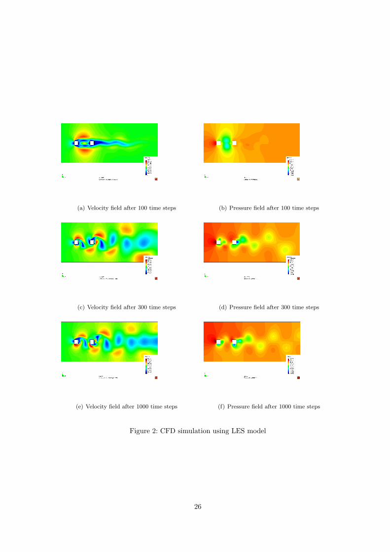
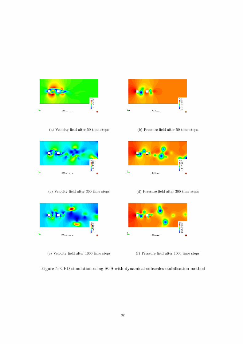
µ , where ρ0 is the fluid density andµ is kinematic viscosity. The mesh used to perform computation is showed in Figure (1). Themesh consists of 14171 nodes and 27508 triangular linear elements. Furthermore, there havebeen consider finer part of mesh around struts where we are interested to capture all behaviorof turbulent flow. The coarser part of the mesh is used in the end of domain. This is usualpicture of mesh because with this we avoid instabilities that can be appear when vortices passboundaries. The time step size used in the computation for first case of landing gear struts withα = 0o is δt = 0.0001. This time step allows us to be between 10 and 100 for ratio betweentime step and critical time step. In figure (2) we can see the velocity and pressure field fordifferent time steps. Pictures shows behavour of turbulent flows around two struts using LESmodel. Getting the velocity field for current problem we applied Fourier transform of velocitycomponents in x and y direction which are tracked in one point between two struts. In figures(3)− (4) we can see the velocity function for a point between two struts and Fourier transformof that function. As we can see in the pictures LES model recovers only main frequencies of theflow generated from large eddies and with that we cannot see the real picture of the turbulentflow. In figure (5) we applied SGS stabilisation technique with dynamical subscales for the sameproblem. We can see the velocity and pressure field in the Figure (5). Getting the velocity fieldfor the problem, we applied Fourier transform for the velocity (x and y component) which isobtained tracking the point between two struts (see in Figures (6) − (7)) As we can see inthese figures the SGS with dynamical subscales include contribution from subscales and withthat gives better approximation of turbulent flow. The aim of these figures is to show howinclusion of subscales in SGS with dynamical subscales recover much more frequencies for thesame point. This conclusion is very useful for further calculation of Litghill’ tensor where weused velocity obtained from CFD simulation
24

Figure 1: Structure of mesh for struts with α = 0o
25
(a) Velocity field after 100 time steps (b) Pressure field after 100 time steps
(c) Velocity field after 300 time steps (d) Pressure field after 300 time steps
(e) Velocity field after 1000 time steps (f) Pressure field after 1000 time steps
Figure 2: CFD simulation using LES model
26

0 0.02 0.04 0.06 0.08 0.1 0.12 0.14−20
0
20
40
60
80
100
120
140Velocity evaluation tracking point in time
time[s]
Vel
ocity
[m/s
]
(a) Velocity (x component) tracking for point betwenstruts
0 100 200 300 400 500 600 7000
5
10
15
20
25Fourier transform of velocity in x direction
Hertz[Hz]
Am
pllit
ude
(b) Fourier transform of velocity
0 0.02 0.04 0.06 0.08 0.1 0.12 0.1410
20
30
40
50
60
70
80Velocity evaluation tracking point in time
time[s]
Vel
ocity
[m/s
]
(c) Velocity (x component) tracking for point behindsecond strut
0 100 200 300 400 500 600 7000
0.5
1
1.5
2
2.5Fourier transform of velocity in x direction
Hertz[Hz]
Am
pllit
ude
(d) Fourier transform of velocity
Figure 3: Velocity ( x direction) tracking in point betwen two struts and Fourier transform ofvelocity function for twostruts with α = 0o
27

0 0.02 0.04 0.06 0.08 0.1 0.12 0.14−30
−25
−20
−15
−10
−5
0
5
10
15
20Velocity evaluation tracking point in time
time[s]
Vel
ocity
[m/s
]
(a) Velocity ( y component) tracking for point betwenstruts
0 100 200 300 400 500 600 7000
0.5
1
1.5
2
2.5
3
3.5
4
4.5Fourier transform of velocity in y direction
Hertz[Hz]
Am
pllit
ude
(b) Fourier transform of velocity
0 0.02 0.04 0.06 0.08 0.1 0.12 0.14−80
−60
−40
−20
0
20
40
60
80Velocity evaluation tracking point in time
time[s]
Vel
ocity
[m/s
]
(c) Velocity ( y component) tracking for point behindsecond strut
0 100 200 300 400 500 600 7000
5
10
15
20
25Fourier transform of velocity in y direction
Hertz[Hz]
Am
pllit
ude
(d) Fourier transform of velocity
Figure 4: Velocity ( y direction) tracking in point between two struts and Fourier transform ofvelocity function for twostruts with α = 0o
28
(a) Velocity field after 50 time steps (b) Pressure field after 50 time steps
(c) Velocity field after 300 time steps (d) Pressure field after 300 time steps
(e) Velocity field after 1000 time steps (f) Pressure field after 1000 time steps
Figure 5: CFD simulation using SGS with dynamical subscales stabilisation method
29

0 0.02 0.04 0.06 0.08 0.1 0.12 0.14−100
−50
0
50
100
150
200Velocity evaluation tracking point in time
time[s]
Vel
ocity
[m/s
]
(a) Velocity ( x component) tracking for point betwenstruts
0 100 200 300 400 500 600 7000
2
4
6
8
10
12
14
16
18Fourier transform of velocity in x direction
Hertz[Hz]
Am
pllit
ude
(b) Fourier transform of velocity
0 0.02 0.04 0.06 0.08 0.1 0.12 0.14−100
−50
0
50
100
150
200Velocity evaluation tracking point in time
time[s]
Vel
ocity
[m/s
]
(c) Velocity ( x component) tracking for point behindsecond strut
0 100 200 300 400 500 600 7000
1
2
3
4
5
6
7
8
9
10Fourier transform of velocity in x direction
Hertz[Hz]
Am
pllit
ude
(d) Fourier transform of velocity
Figure 6: Velocity ( x direction) tracking in point and Fourier transform of velocity functionfor twostruts with α = 0o
30

0 0.02 0.04 0.06 0.08 0.1 0.12 0.14−100
−80
−60
−40
−20
0
20
40
60
80Velocity evaluation tracking point in time
time[s]
Vel
ocity
[m/s
]
(a) Velocity ( y component) tracking for point betwenstruts
0 100 200 300 400 500 600 7000
0.5
1
1.5
2
2.5
3Fourier transform of velocity in y direction
Hertz[Hz]
Am
pllit
ude
(b) Fourier transform of velocity
0 0.02 0.04 0.06 0.08 0.1 0.12 0.14−150
−100
−50
0
50
100
150Velocity evaluation tracking point in time
time[s]
Vel
ocity
[m/s
]
(c) Velocity ( y component) tracking for point behindsecond strut
0 100 200 300 400 500 600 7000
1
2
3
4
5
6
7
8
9Fourier transform of velocity in y direction
Hertz[Hz]
Am
pllit
ude
(d) Fourier transform of velocity
Figure 7: Velocity ( y direction) tracking in point and Fourier transform of velocity functionfor twostruts with α = 0o
31
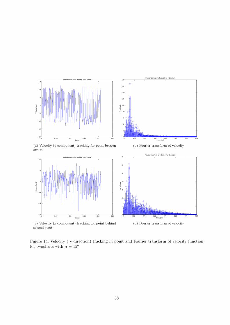
9.2 CFD simulation of generic landing gear struts with horizontal angleα = 15o using LES model and SGS stabilisation method with dynamicalsubscales
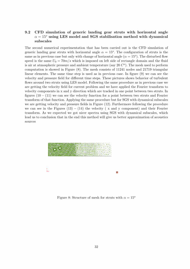
The second numerical experimentation that has been carried out is the CFD simulation ofgeneric landing gear struts with horizontal angle α = 15o. The configuration of struts is thesame as in previous case but only with change of horizontal angle (α = 15o). The disturbed flowspeed is the same U0 = 70m/s which is imposed on left side of rectangle domain and the fluidis air at atmospheric pressure and ambient temperature (say 20 Co). The mesh used to performcomputation is showed in Figure (8). The mesh consists of 11241 nodes and 21719 triangularlinear elements. The same time step is used as in previous case. In figure (9) we can see thevelocity and pressure field for different time steps. These pictures shows behavior of turbulentflows around two struts using LES model. Following the same procedure as in previous case weare getting the velocity field for current problem and we have applied the Fourier transform tovelocity components in x and y direction which are tracked in one point between two struts. Infigures (10 − (11) we can see the velocity function for a point between two struts and Fouriertransform of that function. Applying the same procedure but for SGS with dynamical subscaleswe are getting velocity and pressure fields in Figure (12). Furthermore following the procedurewe can see in the Figures (13) − (14) the velocity ( x and y component) and their Fouriertransform. As we expected we got nicer spectra using SGS with dynamical subscales, whichlead us to conclusion that in the end this method will give us better approximation of acousticssources
Figure 8: Structure of mesh for struts with α = 15o
32
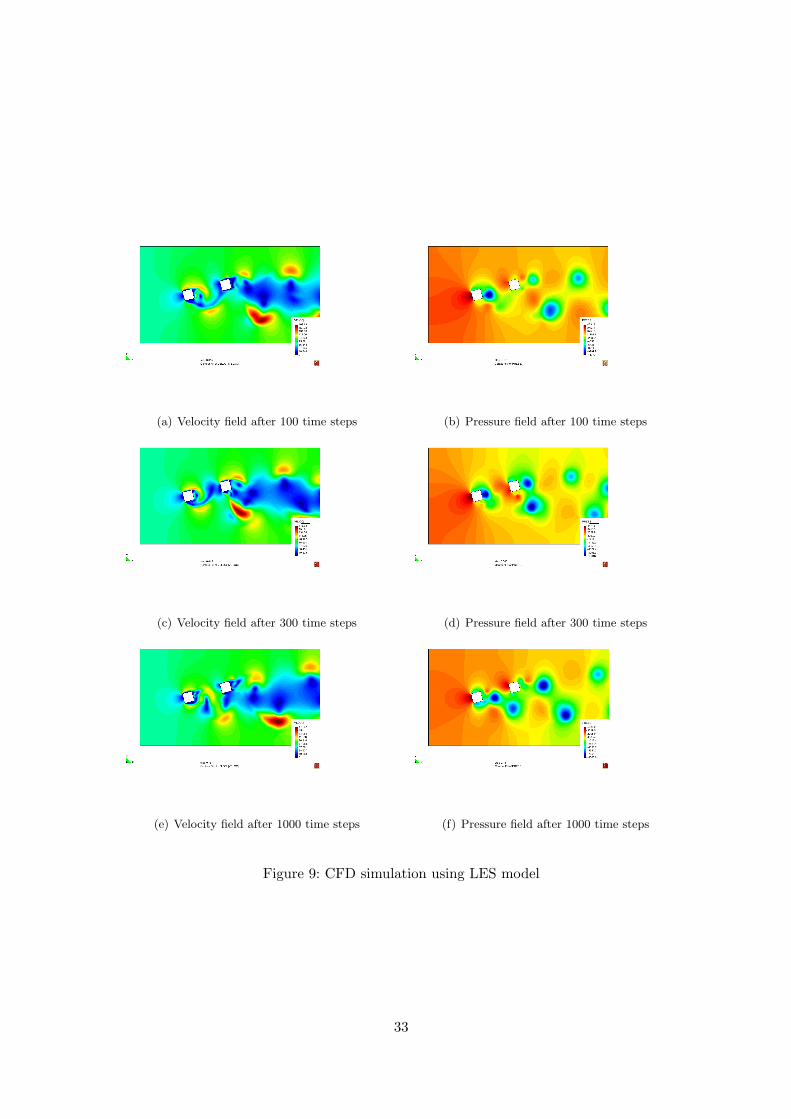
(a) Velocity field after 100 time steps (b) Pressure field after 100 time steps
(c) Velocity field after 300 time steps (d) Pressure field after 300 time steps
(e) Velocity field after 1000 time steps (f) Pressure field after 1000 time steps
Figure 9: CFD simulation using LES model
33

0 0.05 0.1 0.15 0.2 0.25−40
−30
−20
−10
0
10
20
30
40
50
60
time[s]
Vel
ocity
[m/s
]
(a) Velocity (x component) tracking for point betwenstruts
0 100 200 300 400 500 600 7000
5
10
15
Hertz[Hz]
Am
pllit
ude
(b) Fourier transform of velocity
0 0.05 0.1 0.15 0.2 0.25−20
0
20
40
60
80
100
120
time[s]
Vel
ocity
[m/s
]
(c) Velocity (x component) tracking for point behindsecond strut
0 100 200 300 400 500 600 7000
2
4
6
8
10
12
Hertz[Hz]
Am
pllit
ude
(d) Fourier transform of velocity
Figure 10: Velocity ( x direction) tracking in point and Fourier transform of velocity functionfor twostruts with α = 15o
34

0 0.05 0.1 0.15 0.2 0.25−150
−100
−50
0
50
100Velocity(y component) evaluation tracking point in time
time[s]
Vel
ocity
[m/s
]
(a) Velocity (y component) tracking for point betwenstruts
0 100 200 300 400 500 600 7000
5
10
15
20
25
30
35
40
45Fourier transform of velocity in y direction
Hertz[Hz]
Am
pllit
ude
(b) Fourier transform of velocity
0 0.05 0.1 0.15 0.2 0.25−80
−60
−40
−20
0
20
40
60Velocity(y component) evaluation tracking point in time
time[s]
Vel
ocity
[m/s
]
(c) Velocity (x component) tracking for point behindsecond strut
0 100 200 300 400 500 600 7000
5
10
15
20
25Fourier transform of velocity in y direction
Hertz[Hz]
Am
pllit
ude
(d) Fourier transform of velocity
Figure 11: Velocity ( y direction) tracking in point and Fourier transform of velocity functionfor twostruts with α = 15o
35

(a) Velocity field after 100 time steps (b) Pressure field after 100 time steps
(c) Velocity field after 300 time steps (d) Pressure field after 300 time steps
(e) Velocity field after 1000 time steps (f) Pressure field after 1000 time steps
Figure 12: CFD simulation using SGS with dynamical subscales
36

0 0.05 0.1 0.15 0.2 0.25−100
−50
0
50
100
150Velocity evaluation tracking point in time
time[s]
Vel
ocity
[m/s
]
(a) Velocity (x component) tracking for point betwenstruts
0 100 200 300 400 500 600 7000
1
2
3
4
5
6
7
8
9Fourier transform of velocity in x direction
Hertz[Hz]
Am
pllit
ude
(b) Fourier transform of velocity
0 0.05 0.1 0.15 0.2 0.25−40
−20
0
20
40
60
80
100
120
140Velocity evaluation tracking point in time
time[s]
Vel
ocity
[m/s
]
(c) Velocity (x component) tracking for point behindsecond strut
0 100 200 300 400 500 600 7000
1
2
3
4
5
6
7
8Fourier transform of velocity in x direction
Hertz[Hz]
Am
pllit
ude
(d) Fourier transform of velocity
Figure 13: Velocity ( x direction) tracking in point and Fourier transform of velocity functionfor twostruts with α = 15o
37
0 0.05 0.1 0.15 0.2 0.25−200
−150
−100
−50
0
50
100
150Velocity evaluation tracking point in time
time[s]
Vel
ocity
[m/s
]
(a) Velocity (y component) tracking for point betwenstruts
0 100 200 300 400 500 600 7000
2
4
6
8
10
12
14
16
18Fourier transform of velocity in y direction
Hertz[Hz]
Am
pllit
ude
(b) Fourier transform of velocity
0 0.05 0.1 0.15 0.2 0.25−150
−100
−50
0
50
100Velocity evaluation tracking point in time
time[s]
Vel
ocity
[m/s
]
(c) Velocity (x component) tracking for point behindsecond strut
0 100 200 300 400 500 600 7000
1
2
3
4
5
6
7Fourier transform of velocity in y direction
Hertz[Hz]
Am
pllit
ude
(d) Fourier transform of velocity
Figure 14: Velocity ( y direction) tracking in point and Fourier transform of velocity functionfor twostruts with α = 15o
38

9.3 Acoustics sources generated by a single cylinder at Re=500
We consider the case of a two-dimensional cylinder with diameter D=0.0049 m embedded ina flow with free stream velocity in Cartesian coordinates (U0,0). We will concentrate here inthe case where the flow looses its steadiness as well as its up-and-down symmetry and a wakeof alternating vortices is formed behind the cylinder. The set of these shed vortices is knownas the von Karman vortex street. Vortex shedding induces lift fluctuations on the cylinder,which lead to the radiation of sound having a dipole pattern. The radiated sound is knownas aeolian tone. The two-dimensional incompressible Navier-Stokes equations have been solvedusing Subgrid Scale Stabilisation with quasi-static subscales. We remind that this approachallows to use equal interpolation for the velocity and the pressure. In the Figure (15) we cansee an unstructured mesh of linear triangular elements which consists of 20032 points and 39318elements. In the Figure (16) we can see the velocity field for different time steps which describebehavior of the turbulent flow after the cylinder. In Figure (17) a snapshots of the acousticsource term s(x, ω). This term rapidly decrease to zero when moving away from the cylinder.This fact is of crucial importance because it actually justifies the acoustic analogy approaches,which are based on a separation between an acoustic source region and a wave propagatingone. The acoustics sources field has been computed according to the methodology described inSection 8.
Figure 15: Mesh for one cylinder
39

(a) Velocity field after 200 time steps (b) Pressure field after 300 time steps
(c) Velocity field after 400 time steps (d) Pressure field after 750 time steps
(e) Velocity field after 1000 time steps (f) Pressure field after 1500 time steps
Figure 16: Velocity field for one cylinder
40
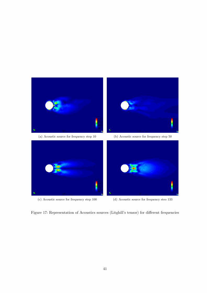
(a) Acoustic source for frequency step 10 (b) Acoustic source for frequency step 50
(c) Acoustic source for frequency step 100 (d) Acoustic source for frequency steo 133
Figure 17: Representation of Acoustics sources (Litghill’s tensor) for different frequencies
41

9.4 Acoustics sources generated by parallel cylinders at Re=1000
We address the computation of the acoustics sources generated by a viscous flow past twoparallel cylinders. Two cylinders of diameter D=0.0049 m are immersed in a flow moving atspeed U0=49 m/s. the characteristic Reynolds number of the problem is given by Re = ρ0U0D
µ ,where ρ is density of air and µ is kinematic viscosity. We will show that vortices are periodicallyshed behind the two cylinders. However, due to the fact that these vortices become antiphasefrom one cylinder to the other, the resulting acoustics sources will considerably differ fromthe single cylinder. The CFD simulation has been performed in a unstructured mesh whichis presented in Figure (18) with 22748 points and 44596 triangular linear elements. Againwe use refinment of the mesh close to cylinders and coarse part in the end of the domain toavoid instabilities. Also the Subgrid Scale Stabilisation method with quasi-static subscales isused for the CFD calculation. The time step size used in the computation is δt = 0.00025s.Once the initial transients have been surpassed, an almost periodic flows is established withvortices being sheded past both cylinders as we can see on Figure (19). It is worthwile tocomment that although the wake sometimes looses its symmetry downstream as time evolves,the vortex shedding remains periodic and antiphase between both cylinders. In what concernsthe acoustic sources field, it has again been computed using the procedure described in Section8. We actually do not know if the presence of the second cylinder may alter the vortex sheddingfrequency when comparing with an analogous single cylinder case, but it certainly increasesthe complexity of the CFD simulation and representation of acoustics sources.
Figure 18: Structure of mesh for two cylinders
42
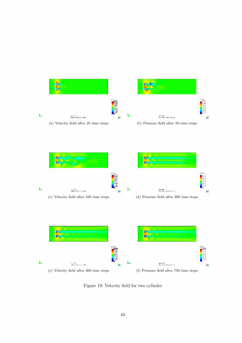
(a) Velocity field after 25 time steps (b) Pressure field after 50 time steps
(c) Velocity field after 100 time steps (d) Pressure field after 200 time steps
(e) Velocity field after 300 time steps (f) Pressure field after 750 time steps
Figure 19: Velocity field for two cylinder
43

(a) Acoustic source for frequency step 335 (b) Acoustic source for frequency step 440
(c) Acoustic source for frequency step 682 (d) Acoustic source for frequency steo 900
Figure 20: Representation of Acoustics sources (Litghill’s tensor) for different frequencies
44

10 Conclusions
In this paper, a numerical formulation to solve the Navier-Stokes equations that consists ona stabilized finite element method and calculation of acoustics sources (Litghill’s tensor) hasbeen presented. Its design is based on the variational multiscale framework which is derivedfrom a splitting of the unknown into two parts, a finite element component and a subscalethat corresponds to the part of the unknown that cannot be captured by the discretization.The crucial point in this approach resides in the subscale approximation. The most importantaspects of this formulation are that it allows to use equal interpolation for all the unknownswithout having to satisfy the inf-sup conditions. Furthermore, it is stable and optimally con-vergent in a norm that is meaningful for any value of the physical parameters of the fluid. Theapproximation of the subscales leads to the introduction of some stabilization parameters thatneed to be proposed. An interesting point of this work is that these parameters have been de-signed based on the stability and convergence analysis of the method. The time integration andlinearization of the problem considered here is the simplest possible which leads to a methodeasy to implement but without losing any robustness and convergence properties. Numericalresults show our prediction that the approximation of subscales will give better representationof turbulent flow and also better approximation of velocity field which lead to better acousticssourse representation. The numerical experimentation presented in this article validates thesestatements and the theoretical development of the method.
11 Future work
Some type of analysis should be performed in order to know the degree of precision of thecomputed acoustic field. Although the validity of Lighthills acoustic analogy has been exten-sively analysed for the continuous case by some authors, further work is needed to asses similarresults for the herein presented and similar numerical CAA approaches. In the line of the pre-vious point, it would be worthwhile to implement Ristorcellis closure and compare its degreeof accuracy with Lighthills acoustic analogy for some benchmark problems. It is important tosee how much the methods we presented will affect calculation of inhomogeneous Helmholtzequation. It’s worth to try with differnet stabilisation approaches of Helmholtz equation andresults obtained in this work to get better approximation of acoustic pressure field. It wouldbe worthwhile to check if the various SGS methods constitute suitable approximations to theNavier-Stokes equations. Since now it has only been proved that the Galerkin finite elementmethod for problems with periodic or Dirichlet boundary conditions satisfy this assumption.
Acknowledgements
V. Jazarevic would like to aknowledge the support received from the Universitat Politecnicade Catalunya (UPC).
References
[1] R. Codina. Stabilization of incompressibility and convection through orthogonal sub-scalesin finite element methods. Computer Methods in Applied Mechanics and Engineering,190:1579–1599, 1965.
45

[2] R. Codina. On stabilized finite element methods for linear systems of convection-diffusion-reaction equations. Computer Methods in Applied Mechanics and Engineering, 188:61–82,2000.
[3] Germano. differential filters for the large eddy simulation of turbulent flows. Phys. fluids,,29(6):1755–1757, 1986.
[4] T.J.R. Hughes. Multiscale phenomena: Green’s function, the Dirichlet-to-Neumann formu-lation, subgrid scale models, bubbles and the origins of stabilized formulations. ComputerMethods in Applied Mechanics and Engineering, 127:387–401, 1995.
[5] J. Oden J. Guermond and S. Prudhomme. Mathematical persspectives on large eddysimulation models for turbulent flows. Technical report, 2007.
[6] A Kolmogorov. The local structure of turbilence in incompressible viscous fluids for verylarge reynolds number. Dokl. Akad. Sci. Nauk. SSSR, 190:299–330, 1941.
[7] D. Lilly. The representation of small-scale turbulence theory in numerical simulation ex-periments. H. Goldstine, editor, Proc. IBM Scientific Computing Symp. on EnvironmentalSciences, 1967.
[8] A. Monin and A. Yaglom. Statistical fluid mechanics: Mechanics of turbulence. voluumeii. 1975.
[9] S. Pope. Turbulent flows. 38, 2000.
[10] O. Guasch R. Codina, J. Principe and S. Badia. Time dependent subscales in the sta-bilisedfinite element approximation of incompressible flow problems. Computer Methodsin Applied Mechanics and Engineering, 196(21-24):2413–2430, 2007.
[11] R.Codina. Stabilized finite element approximation of transient incompressible flows us-ing orthogonal subscales. Computer Methods in Applied Mechanics and Engineering,191:4295–4321, 2002.
[12] L. Mazzei T. Hughes and K. Jansen. Large eddy simulation and the variational multiscalemethod. Comput. Visual. Sci., 3:47–59, 2000.
[13] L. Mazzei T.Hughes, G. Feijoo and J. Quincy. The variational multiscale method-aparadigm for computational mechanics. Computer Methods in Applied Mechanics andEngineering, 166:3–24, 1998.
46