
Ketan Savla - arXiv2 Mohammad Motie, Ketan Savla performance. Within this application context, one...
27
Noname manuscript No. (will be inserted by the editor) Service Rate, Busy Period & Throughput Analysis of a Horizontal Traffic Queue Mohammad Motie · Ketan Savla Abstract We consider a horizontal traffic queue (HTQ) on a periodic road segment, where vehicles arrive according to a spatio-temporal Poisson process, and depart after traveling a distance that is sampled independently and identically from a spatial distribution. When inside the queue, the speed of a vehicle is proportional to a power m> 0 of the distance to the vehicle in front. The service rate of HTQ is equal to the sum of the speeds of the vehicles, and has a complex dependency on the state (vehicle locations) of the system. We show that the service-rate increases (resp., decreases) in between arrivals and departures for m< 1 (resp., m> 1) case. For a given initial condition, we define the throughput of such a queue as the largest arrival rate under which the queue length remains bounded. We extend the busy period calculations for M/G/1 queue to our setting, including for non-empty initial condition. These calculations are used to prove that the throughput for m = 1 case is equal to the inverse of the time required to travel average total distance by a solitary vehicle in the system, and also to derive a probabilistic upper bound on the queue length over a finite time horizon for the m> 1 case. Finally, we study throughput under a release control policy, where the additional expected waiting time caused by the control policy is interpreted as the magnitude of the perturbation to the arrival process. We derive a lower bound on throughput for a given combination of maximum allowable perturbation, for m< 1 and m> 1 cases. In particular, if the allowable perturbation is sufficiently large, then this lower bound grows unbounded as m → 0 + . Illustrative simulation results are also presented. 1 Introduction We consider a horizontal traffic queue (HTQ) on a periodic road segment, where vehicles arrive according to a spatio-temporal Poisson process, and depart the queue after traveling a distance that is sampled independently and identically from a spatial distribution. When inside the queue, the speed of a vehicle is proportional to a power m> 0 of the distance to the vehicle in front. For a given initial condition, we define the throughput of such a queue as the largest arrival rate under which the queue length remains bounded. We provide rigorous analysis for the service rate, busy period distribution, and throughput of the proposed HTQ. Our motivation for studying HTQ comes from advancements in connected and autonomous vehi- cle technologies that allow to program individual vehicles with rules that can optimize system level M. Motie Sonny Astani Department of Civil and Environmental Engineering University of Southern California E-mail: [email protected] K. Savla Sonny Astani Department of Civil and Environmental Engineering University of Southern California E-mail: [email protected] arXiv:1604.06144v2 [math.DS] 23 May 2016
Transcript of Ketan Savla - arXiv2 Mohammad Motie, Ketan Savla performance. Within this application context, one...

Noname manuscript No.(will be inserted by the editor)
Service Rate, Busy Period & Throughput Analysis of a Horizontal TrafficQueue
Mohammad Motie · Ketan Savla
Abstract We consider a horizontal traffic queue (HTQ) on a periodic road segment, where vehiclesarrive according to a spatio-temporal Poisson process, and depart after traveling a distance that issampled independently and identically from a spatial distribution. When inside the queue, the speedof a vehicle is proportional to a power m > 0 of the distance to the vehicle in front. The service rateof HTQ is equal to the sum of the speeds of the vehicles, and has a complex dependency on the state(vehicle locations) of the system. We show that the service-rate increases (resp., decreases) in betweenarrivals and departures for m < 1 (resp., m > 1) case. For a given initial condition, we define thethroughput of such a queue as the largest arrival rate under which the queue length remains bounded.We extend the busy period calculations for M/G/1 queue to our setting, including for non-empty initialcondition. These calculations are used to prove that the throughput for m = 1 case is equal to theinverse of the time required to travel average total distance by a solitary vehicle in the system, and alsoto derive a probabilistic upper bound on the queue length over a finite time horizon for the m > 1 case.Finally, we study throughput under a release control policy, where the additional expected waiting timecaused by the control policy is interpreted as the magnitude of the perturbation to the arrival process.We derive a lower bound on throughput for a given combination of maximum allowable perturbation,for m < 1 and m > 1 cases. In particular, if the allowable perturbation is sufficiently large, then thislower bound grows unbounded as m→ 0+. Illustrative simulation results are also presented.
1 Introduction
We consider a horizontal traffic queue (HTQ) on a periodic road segment, where vehicles arrive accordingto a spatio-temporal Poisson process, and depart the queue after traveling a distance that is sampledindependently and identically from a spatial distribution. When inside the queue, the speed of a vehicleis proportional to a power m > 0 of the distance to the vehicle in front. For a given initial condition, wedefine the throughput of such a queue as the largest arrival rate under which the queue length remainsbounded. We provide rigorous analysis for the service rate, busy period distribution, and throughputof the proposed HTQ.
Our motivation for studying HTQ comes from advancements in connected and autonomous vehi-cle technologies that allow to program individual vehicles with rules that can optimize system level
M. MotieSonny Astani Department of Civil and Environmental EngineeringUniversity of Southern CaliforniaE-mail: [email protected]
K. SavlaSonny Astani Department of Civil and Environmental EngineeringUniversity of Southern CaliforniaE-mail: [email protected]
arX
iv:1
604.
0614
4v2
[m
ath.
DS]
23
May
201
6
2 Mohammad Motie, Ketan Savla
performance. Within this application context, one can interpret the results of this paper as rigorouslycharacterizing the impact of a parametric class of car-following behavior on system throughput.
In the linear case (m = 1), i.e., when the speed of every vehicle is proportional to the distance tothe vehicle directly in front, the periodicity of the road segment implies that the sum of the speeds ofthe vehicles is proportional to the total length of the road segment, i.e., it is constant. This featureallows us to exploit the equivalence between workload and queue length to show that, independent ofthe initial condition and almost surely, the throughput is the inverse of the time required by a solitaryvehicle to travel average distance.
In the non-linear case (m 6= 1), the cumulative service rate of HTQ queue is constant if and only if allthe inter-vehicle distances are equal. For all other inter-vehicle configurations, we show that the servicerate is strictly decreasing (resp., strictly increasing) in the super-linear, i.e., m > 1 (resp., sub-linear,i.e., m < 1) case. The service rate exhibits an another contrasting behavior in the sub- and super-linearregimes. In the super-linear case, the service rate is maximum (resp., minimum) when all the vehiclesare co-located (resp., when the inter-vehicle distances are equal), and vice-versa for the sub-linear case.Using a combination of these properties, we prove that, when the length of the road segment is at mostone, the throughput in the super-linear (resp., sub-linear) case is upper (resp., lower) bounded by thethroughput for the linear case.
We prove the remaining bounds on the throughput for the non-linear case as follows. The stan-dard calculations for joint distributions of duration and number of arrivals during a busy period forM/G/1 queue are extended to the HTQ setting, including for non-empty initial conditions. These jointdistributions are used to derive probabilistic upper bounds on queue length over finite time horizonsfor HTQ for the m > 1 case. Such bounds are optimized to get lower bounds on throughput definedover finite time horizons. Simulation results show good comparison between such lower bounds andnumerical estimates.
We also analyze throughput in the sub-linear and super-linear cases under perturbation to the arrivalprocess, which is attributed to the additional expected waiting time induced by a release control policythat adds appropriate delay to the arrival times to ensure a desired minimum inter-vehicle distance4 > 0 at the time of a vehicle joining the HTQ. Since the minimum inter-vehicle distance is non-decreasing in between arrivals and jumps, this implies an upper bound on the queue length whichis inversely proportional to 4. We derive a lower bound on throughput for a given combination ofmaximum allowable perturbation. In particular, if the allowable perturbation is sufficiently large, thenthis lower bound grows unbounded, as m→ 0+.
Queueing models have been used to model and analyze traffic systems. The focus here has beenprimarily on vertical queues, under which vehicles travel at maximum speed until they hit a congestionspot where all vehicles queue on top of each other. The queue length and waiting time of a minor trafficstream at an unsignalized intersection where major traffic stream has high priority is studied in [20] and[8]. In [9], a vertical single server queue is utilized to model the queue length distribution at signalizedintersections. In [11], a state-dependent queuing system is used to model vehicular traffic flow wherethe service rate depends on the number of vehicles on each road link.
On the other hand, the horizontal traffic queue terminology has been primarily used to study macro-scopic traffic flow, e.g., see [10]. While such models capture the macroscopic relationship between trafficflow and density, a rigorous description and analysis of an underlying queue model is lacking. Indeed, tothe best of our knowledge, there is no prior work on the analysis of a traffic queue model that explicitlyincorporates car-following behavior.
The proposed HTQ has an interesting connection with processor sharing (PS) queues, and thisconnection does not seem to have been documented before. A characteristic feature of PS queues is thatall the outstanding jobs receive service simultaneously, while keeping the total service rate of the serverconstant. The simplest model is where the service rate for an individual job is equal to 1/N , where Nis the number of outstanding jobs. In our proposed system, one can interpret the road segment as aserver simultaneously providing service to all the vehicles, with the service rate of an individual vehicleequal to its speed. This natural analogy between HTQ and PS queues, to the best of our knowledge,
Service Rate, Busy Period & Throughput Analysis of a Horizontal Traffic Queue 3
was reported for the first time in our recent work [15]. The 1/N rule applied to our setting implies thatall the vehicles travel with the same speed. Clearly, such a rule, or even the general discriminatory PSdisciplines, e.g., see [14], are not applicable to the car following models considered in this paper. Indeed,the proposed HTQ is best described as a state-dependent PS queue.
In the PS queue literature, the focus has been on the sojourn time and queue length distribution.For example, see [17] and [21] for M/G/1-PS queue and [6] for G/G/1-PS queue. Fluid limit analysis forPS queue is provided in [4] and [7]. However, relatively less attention has been paid to the throughputanalysis of state-dependent PS queues. In [16,12,5], throughput analysis for state-dependent PS queuesis provided, where throughput is defined as the quantity of work achieved by the server per unit of time.Stability analysis for a single server queue with workload-dependent service and arrival rate is providedin [2] and [3]. However, the dependence of service rate on the system state in the HTQ proposed in thecurrent paper is complex, and hence none of these results are readily applicable.
In summary, there are several novel contributions of the paper. First, we propose a novel horizontaltraffic queue and place it in the context of processor-sharing queues and state-dependent queues. Weestablish monotonicity properties of service rates in between jumps (i.e., arrivals and departures), andderive bounds on change in service rates at jumps. Second, we adapt busy period calculations for M/G/1queue to our current setup, including for non-empty initial conditions. These results allow us to providetight results for throughput in the linear case, and probabilistic bounds on queue length over finitetime horizon in the super-linear case. We also study throughput under a batch release control policy,whose effect is interpreted as a perturbation to the arrival process. We provide lower bound on thethroughput for a maximum permissible perturbation for sub- and super-linear cases. In particular, weshow that, for sufficiently large perturbation, this lower bound grows unbounded as m → 0+. It isinteresting to compare our analytical results with simulation results, which suggest a sharp transitionin the throughput from being unbounded in the sub-linear regime to being bounded in the super-linearregime. While our analytical results do not exhibit such a phase transition yet, their novelty is inproviding rigorous estimates of any kind on the throughput of horizontal traffic queues under nonlinearcar following models.
The rest of the paper is organized as follows. We conclude this section with key notations to be usedthroughout the paper. The setting for the proposed horizontal traffic queue and formal definition ofthroughput are provided in Section 2. Section 3 contains useful properties on the dynamics in servicerate in between and during jumps. Key busy period properties for the M/G/1 queue are extended tothe HTQ case in Section 4.2. Throughput analysis is reported in Section 5. Simulations are presentedin 6. Concluding remarks and directions for future work are presented in Section 7. A few technicalintermediate results are collected in the appendix.
Notations
Let R, R+, and R++ denote the set of real, non-negative real, and positive real numbers, respectively.Let N be the set of natural numbers. If x1 and x2 are of the same size, then x1 ≥ x2 implies element-wise inequality between x1 and x2. If x1 and x2 are of different sizes, then x1 ≥ x2 implies inequalityonly between elements which are common to x1 and x2 – such a common set of elements will bespecified explicitly. For a set J , let int(J ) and |J | denote the interior and cardinality of J , respectively.Given a ∈ R, and b > 0, we let mod (a, b) := a − bab cb. Let SLN be the N − 1-simplex over L, i.e.,
SLN ={x ∈ RN+ |
∑Ni=1 xi = L
}. When L = 1, we shall use the shorthand notation SN . When referring
to the set {1, . . . , N}, for brevity, we let the indices i = −1 and i = N + 1 correspond to i = N andi = 1 respectively. Also, for p, q ∈ SN , we let D(p||q) denote the K-L divergence of q from p, i.e.,
D(p||q) :=∑Ni=1 pi log (pi/qi). We also define a permutation matrix, P− ∈ {0, 1}N×N , as follows:
P− :=
[0TN−1 1IN−1 0N−1
]
4 Mohammad Motie, Ketan Savla
where 0N and 1N stand for vectors of size N , all of whose entries are zero and one, respectively. Weshall drop N from 0N and 1N whenever it is clear from the context.
2 The Horizontal Traffic Queue (HTQ) Setup
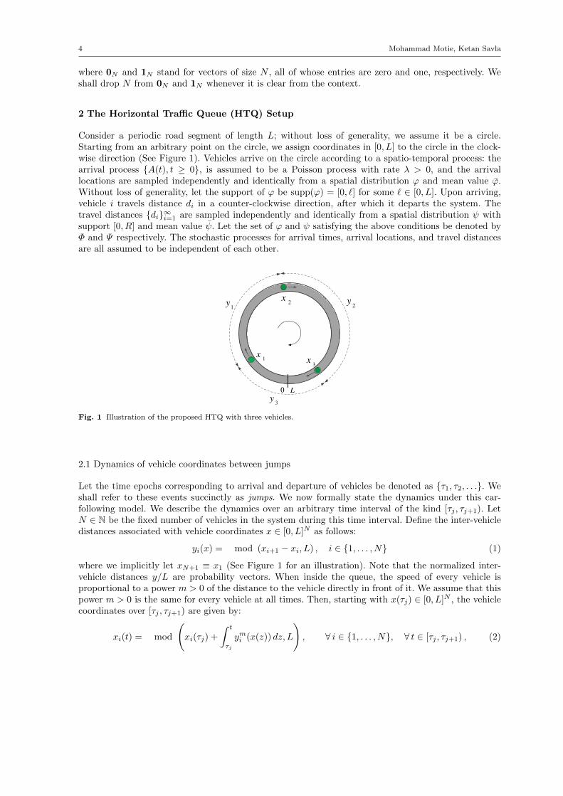
Consider a periodic road segment of length L; without loss of generality, we assume it be a circle.Starting from an arbitrary point on the circle, we assign coordinates in [0, L] to the circle in the clock-wise direction (See Figure 1). Vehicles arrive on the circle according to a spatio-temporal process: thearrival process {A(t), t ≥ 0}, is assumed to be a Poisson process with rate λ > 0, and the arrivallocations are sampled independently and identically from a spatial distribution ϕ and mean value ϕ.Without loss of generality, let the support of ϕ be supp(ϕ) = [0, `] for some ` ∈ [0, L]. Upon arriving,vehicle i travels distance di in a counter-clockwise direction, after which it departs the system. Thetravel distances {di}∞i=1 are sampled independently and identically from a spatial distribution ψ withsupport [0, R] and mean value ψ. Let the set of ϕ and ψ satisfying the above conditions be denoted byΦ and Ψ respectively. The stochastic processes for arrival times, arrival locations, and travel distancesare all assumed to be independent of each other.
HTQ1 Release Control Policy
HTQ2HTQ1
HTQ2
(a) (b)
1x
2x
3x
1y 2y
3y0 L
' HTQ1
HTQ2
HTQ1Release Control
Policy
HTQ2
1x
2x
3x
1y 2y
3y0 L
1x
2x
3x
1y 2y
3y0 L
1x
2x
3x
1y 2y
3y0 L
Fig. 1 Illustration of the proposed HTQ with three vehicles.
2.1 Dynamics of vehicle coordinates between jumps
Let the time epochs corresponding to arrival and departure of vehicles be denoted as {τ1, τ2, . . .}. Weshall refer to these events succinctly as jumps. We now formally state the dynamics under this car-following model. We describe the dynamics over an arbitrary time interval of the kind [τj , τj+1). LetN ∈ N be the fixed number of vehicles in the system during this time interval. Define the inter-vehicledistances associated with vehicle coordinates x ∈ [0, L]N as follows:
yi(x) = mod (xi+1 − xi, L) , i ∈ {1, . . . , N} (1)
where we implicitly let xN+1 ≡ x1 (See Figure 1 for an illustration). Note that the normalized inter-vehicle distances y/L are probability vectors. When inside the queue, the speed of every vehicle isproportional to a power m > 0 of the distance to the vehicle directly in front of it. We assume that thispower m > 0 is the same for every vehicle at all times. Then, starting with x(τj) ∈ [0, L]N , the vehiclecoordinates over [τj , τj+1) are given by:
xi(t) = mod
(xi(τj) +
∫ t
τj
ymi (x(z)) dz, L
), ∀ i ∈ {1, . . . , N}, ∀ t ∈ [τj , τj+1) , (2)
Service Rate, Busy Period & Throughput Analysis of a Horizontal Traffic Queue 5
Remark 1 It is easy to see that the clock-wise ordering of the vehicles is invariant under (1)-(2).
The dynamics in inter-vehicle distances is given by:
yi = ymi+1 − ymi , i ∈ {1, . . . , N} (3)
where we implicitly let yN+1 ≡ y1.
2.2 Change in vehicle coordinates during jumps
Let x(τ−j ) =(x1(τ−j ), . . . , xN (τ−j )
)∈ [0, L]N be the vehicle coordinates just before the jump at τj . If
the jump corresponds to the departure of vehicle k ∈ {1, . . . , N}, then the coordinates of the vehiclesx(τj) = (x1(τj), . . . , xN−1(τj)) ∈ [0, L]N−1 after re-ordering due to the jump, for i ∈ {1, . . . , N −1}, aregiven by:
xi(τj) =
xi(τ
−j ) i ∈ {1, . . . , k − 1}
xi+1(τ−j ) i ∈ {k + 1, . . . , N − 1} .
Analogously, if the jump corresponds to arrival of a vehicle at location z ∈ [0, `] in between thelocations of the k-th and k + 1-th vehicles at time τ−j , then the coordinates of the vehicles x(τj) =
(x1(τj), . . . , xN+1(τj)) ∈ [0, L]N+1 after re-ordering due to the jump, for i ∈ {1, . . . , N + 1}, are givenby:
xk+1(τj) = z
xi(τj) =
xi(τ
−j ) i ∈ {1, . . . , k}
xi−1(τ−j ) i ∈ {k + 2, . . . , N + 1} .
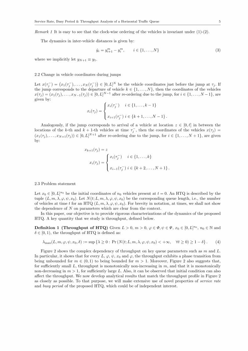
2.3 Problem statement
Let x0 ∈ [0, L]n0 be the initial coordinates of n0 vehicles present at t = 0. An HTQ is described by thetuple (L,m, λ, ϕ, ψ, x0). Let N(t;L,m, λ, ϕ, ψ, x0) be the corresponding queue length, i.e., the numberof vehicles at time t for an HTQ (L,m, λ, ϕ, ψ, x0). For brevity in notation, at times, we shall not showthe dependence of N on parameters which are clear from the context.
In this paper, our objective is to provide rigorous characterizations of the dynamics of the proposedHTQ. A key quantity that we study is throughput, defined below.
Definition 1 (Throughput of HTQ) Given L > 0, m > 0, ϕ ∈ Φ,ψ ∈ Ψ , x0 ∈ [0, L]n0 , n0 ∈ N andδ ∈ [0, 1), the throughput of HTQ is defined as:
λmax(L,m,ϕ, ψ, x0, δ) := sup {λ ≥ 0 : Pr (N(t;L,m, λ, ϕ, ψ, x0) < +∞, ∀t ≥ 0) ≥ 1− δ} . (4)
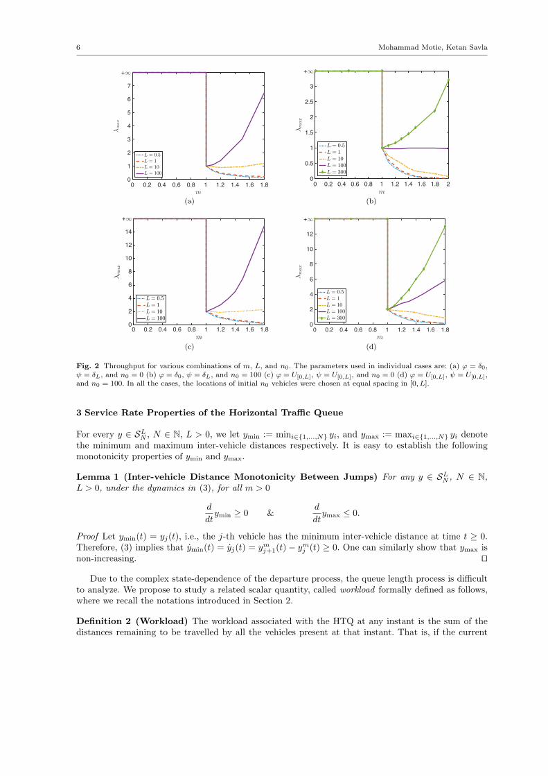
Figure 2 shows the complex dependency of throughput on key queue parameters such as m and L.In particular, it shows that for every L, ϕ, ψ, x0 and ϕ, the throughput exhibits a phase transition frombeing unbounded for m ∈ (0, 1) to being bounded for m > 1. Moreover, Figure 2 also suggests that,for sufficiently small L, throughput is monotonically non-increasing in m, and that it is monotonicallynon-decreasing in m > 1, for sufficiently large L. Also, it can be observed that initial condition can alsoaffect the throughput. We now develop analytical results that match the throughput profile in Figure 2as closely as possible. To that purpose, we will make extensive use of novel properties of service rateand busy period of the proposed HTQ, which could be of independent interest.
6 Mohammad Motie, Ketan Savla
0 0.2 0.4 0.6 0.8 1 1.2 1.4 1.6 1.8m
0
1
2
3
4
5
6
7
+∞
λmax
L = 0.5L = 1L = 10L = 100
(a)
0 0.2 0.4 0.6 0.8 1 1.2 1.4 1.6 1.8 2m
0
0.5
1
1.5
2
2.5
3
+∞
λmax
L = 0.5L = 1L = 10L = 100L = 300
(b)
m0 0.2 0.4 0.6 0.8 1 1.2 1.4 1.6 1.8
6m
ax
0
2
4
6
8
10
12
14
+1
L = 0:5L = 1L = 10L = 100
(c)
0 0.2 0.4 0.6 0.8 1 1.2 1.4 1.6 1.8m
0
2
4
6
8
10
12
+∞
λmax
L = 0.5L = 1L = 10L = 100L = 300
(d)
Fig. 2 Throughput for various combinations of m, L, and n0. The parameters used in individual cases are: (a) ϕ = δ0,ψ = δL, and n0 = 0 (b) ϕ = δ0, ψ = δL, and n0 = 100 (c) ϕ = U[0,L], ψ = U[0,L], and n0 = 0 (d) ϕ = U[0,L], ψ = U[0,L],and n0 = 100. In all the cases, the locations of initial n0 vehicles were chosen at equal spacing in [0, L].
3 Service Rate Properties of the Horizontal Traffic Queue
For every y ∈ SLN , N ∈ N, L > 0, we let ymin := mini∈{1,...,N} yi, and ymax := maxi∈{1,...,N} yi denotethe minimum and maximum inter-vehicle distances respectively. It is easy to establish the followingmonotonicity properties of ymin and ymax.
Lemma 1 (Inter-vehicle Distance Monotonicity Between Jumps) For any y ∈ SLN , N ∈ N,L > 0, under the dynamics in (3), for all m > 0
d
dtymin ≥ 0 &
d
dtymax ≤ 0.
Proof Let ymin(t) = yj(t), i.e., the j-th vehicle has the minimum inter-vehicle distance at time t ≥ 0.Therefore, (3) implies that ymin(t) = yj(t) = ymj+1(t)− ymj (t) ≥ 0. One can similarly show that ymax isnon-increasing. ut
Due to the complex state-dependence of the departure process, the queue length process is difficultto analyze. We propose to study a related scalar quantity, called workload formally defined as follows,where we recall the notations introduced in Section 2.
Definition 2 (Workload) The workload associated with the HTQ at any instant is the sum of thedistances remaining to be travelled by all the vehicles present at that instant. That is, if the current
Service Rate, Busy Period & Throughput Analysis of a Horizontal Traffic Queue 7
coordinates and departure coordinates of all vehicles are x ∈ [0, L]N and q ∈ RN+ respectively, withq ≥ x, then the workload is given by:
w(x, q) :=
N∑i=1
(qi − xi).
Since the maximum distance to be travelled by any vehicle from the time of arrival to the timeof departure is upper bounded by R, we have the following simple relationship between workload andqueue length at any time instant:
w(t) ≤ N(t)R , ∀ t ≥ 0 . (5)
An implication of (5) is that unbounded workload implies unbounded queue length in our setting. Weshall use this relationship to establish an upper bound on the throughput. However, a finite workloaddoes not necessarily imply finite queue length. In order to see this, consider the state of the queue withN vehicles, all of whom have distance 1/N remaining to be travelled. Therefore, the workload at thisinstant is 1/N ×N = 1, which is independent of N .
When the workload is positive, its rate of decrease is equal to service rate in between jumps, definednext.
Definition 3 (Service Rate) When the HTQ is not idle, its instantaneous service rate is equal to the
sum of the speeds of the vehicles present in the system at that time instant, i.e., s(x) =∑Ni=1 y
mi (x).
Since the service rate depends only on the inter-vehicle distances, we shall alternately denote it ass(y). For m = 1, s(y) =
∑Ni=1 yi ≡ L, i.e., the service rate is independent of the state of the system, and
is constant in between and during jumps. This property does not hold true in the nonlinear (m 6= 1) case.Nevertheless, one can prove interesting properties for the service rate dynamics. We start by derivingbounds on service rate in between jumps.
Lemma 2 (Bounds on Service Rates) For any y ∈ SLN , N ∈ N, L > 0, under the dynamics in (3),
1. LmN1−m ≤ s(y) ≤ Lm if m > 1;2. Lm ≤ s(y) ≤ LmN1−m if m ∈ (0, 1).
Proof Normalizing the inter-vehicular distances by L, the service rate can be rewritten as
s(y) = LmN∑i=1
(yiL
)m. (6)
Therefore, for m > 1, s(y) ≤ Lm∑Ni=1
yiL = Lm. One can similarly show that, for m ∈ (0, 1), s(y) ≥ Lm.
In order to prove the remaining bounds, we note that∑Ni=1 z
mi is strictly convex in z = [z1, . . . , zN ]
for m > 1, and that the minimum of∑Ni=1 z
mi over z ∈ SN occurs at z = 1/N , and is equal to N1−m.
Similarly, for m ∈ (0, 1),∑Ni=1 z
mi is strictly concave in z, and its maximum over z ∈ SN occurs at
z = 1/N , and is equal to N1−m. Combining these facts with (6), and noting that y/L ∈ SN , gives thelemma. ut
Lemma 3 (Service Rate Monotonicity Between Jumps) For any y ∈ SLN , N ∈ N, L > 0, underthe dynamics in (3),
d
dts(y) ≤ 0 if m > 1 &
d
dts(y) ≥ 0 if m ∈ (0, 1) ,
where the equality holds true if and only if y = LN 1.
8 Mohammad Motie, Ketan Savla
Proof The time derivative of service rate is given by:
d
dts(y) =
d
dt
N∑i=1
ymi = m
N∑i=1
ym−1i yi
= m
N∑i=1
ym−1i
(ymi+1 − ymi
)(7)
where the second equality follows by (3). The result then follows by application of Lemma 12, andby noting that g(z) = zm is a strictly increasing function for all m > 0, and h(z) = zm−1 is strictlydecreasing if m ∈ (0, 1), and strictly increasing if m > 1. ut
The following lemma quantifies the change in service rate due to departure of a vehicle.
Lemma 4 (Change in Service Rate at Departures) Consider the departure of a vehicle thatchanges inter-vehicle distances from y ∈ SLN to y− ∈ SLN−1, for some N ∈ N \ {1}, L > 0. If y1 ≥ 0and y2 ≥ 0 denote the inter-vehicle distances behind and in front of the departing vehicle respectively,at the moment of departure, then the change in service rate due to the departure satisfies the followingbounds:
1. if m > 1, then 0 ≤ s(y−)− s(y) ≤ (y1 + y2)m(1− 21−m
);
2. if m ∈ (0, 1), then 0 ≤ s(y)− s(y−) ≤ min{ym1 , ym2 }.
Proof If m > 1, then(
y1y1+y2
)m+(
y2y1+y2
)m≤ y1
y1+y2+ y2
y1+y2= 1, i.e., s(y−) − s(y) = (y1 + y2)m −
ym1 − ym2 ≥ 0. One can similarly show that s(y)− s(y−) ≥ 0 if m ∈ (0, 1).In order to show the upper bound on s(y−) − s(y) for m > 1, we note that the minimum value of
zm + (1− z)m over z ∈ [0, 1] for m > 1 is 21−m, and it occurs at z = 1/2. Therefore,
s(y−)− s(y) = (y1 + y2)m − ym1 − ym2 = (y1 + y2)m(
1−(
y1y1 + y2
)m−(
y2y1 + y2
)m)≤ (y1 + y2)m
(1− 21−m
)The upper bound on s(y) − s(y−) for m ∈ (0, 1) can be proven as follows. Since ym1 ≤ (y1 + y2)m,
s(y)−s(y−) = ym1 +ym2 −(y1+y2)m ≤ ym2 . Similarly, s(y)−s(y−) ≤ ym1 . Combining, we get s(y)−s(y−) ≤min{ym1 , ym2 }. Note that, in proving this, we nowhere used the fact that m ∈ (0, 1). However, this boundis useful only for m ∈ (0, 1). ut
Remark 2 (Change in Service Rate at Arrivals) The bounds derived in Lemma 4 can be trivially usedto prove the following bounds for change in service rate at arrivals:
1. if m > 1, then 0 ≤ s(y)− s(y+) ≤ (y1 + y2)m(1− 21−m
);
2. if m ∈ (0, 1), then 0 ≤ s(y+)− s(y) ≤ min{ym1 , ym2 },where y1 and y2 are the inter-vehicle distances behind and in front of the arriving vehicle respectively,at the moment of arrival.
The following lemma will facilitate generalization of Lemma 3. In preparation for the lemma, letf(y,m) := m
∑Ni=1 y
m−1i
(ymi+1 − ymi
)be the time derivative of service rate, as given in (7).
Lemma 5 For all y ∈ int(SLN ), N ∈ N \ {1}, L > 0:
∂
∂mf(y,m)|m=1 = −LD
( yL||P− y
L
)≤ 0 (8)
Additionally, if L < e−2, then∂2
∂m2f(y,m)|m=1 ≥ 0 (9)
Moreover, equality holds true in (8) and (9) if and only if y = LN 1.
Service Rate, Busy Period & Throughput Analysis of a Horizontal Traffic Queue 9
Proof Taking the partial derivative of f(y,m) with respect to m, we get that
∂
∂mf(y,m) =
f(y,m)
m+m
N∑i=1
(ym−1i ymi+1 (log yi + log yi+1)− 2y2m−1i log yi
)In particular, for m = 1:
∂
∂mf(y,m)|m=1 = f(y, 1) +
N∑i=1
(yi+1 (log yi + log yi+1)− 2yi log yi)
= L
N∑i=1
yiL
log
(yi−1/L
yi/L
)= −LD
( yL||P− y
L
)where, for the second equality, we used the trivial fact that f(y, 1) = 0. Taking second partial derivativeof f(y,m) w.r.t. m gives:
∂2
∂m2f(y,m) =
N∑i=1
ym−1i log yi(ymi+1 − ymi
)+
N∑i=1
ym−1i
(ymi+1 log yi+1 − ymi log yi
)+
N∑i=1
(ym−1i ymi+1 (log yi + log yi+1)− 2y2m−1i log yi
)+m
N∑i=1
(ym−1i ymi+1 (log yi + log yi+1)
2 − 4y2m−1i log2 yi
)In particular, for m = 1:
∂2
∂m2f(y,m)|m=1 =
N∑i=1
(yi+1 − yi) log yi +
N∑i=1
(yi+1 log yi+1 − yi log yi)
+
N∑i=1
(yi+1 (log yi + log yi+1)− 2yi log yi)
+
N∑i=1
(yi+1(log yi + log yi+1)2 − 4yi log2 yi
)=
N∑i=1
log2 yi (yi+1 − yi) + 2
N∑i=1
log yi (yi+1 log yi+1 + yi+1 − yi log yi − yi) (10)
≥ 0
It is easy to check that, log z, log2 z and z+z log z are strictly increasing, strictly decreasing and strictlydecreasing functions, respectively, for z ∈ (0, e−2). Therefore, Lemma 12 implies that each of the twoterms in (10) is non-negative, and hence the lemma. ut
Lemma 5 implies that, for sufficiently small L, f(y,m) is locally convex in m. One can use thisproperty along with an exact expression for ∂
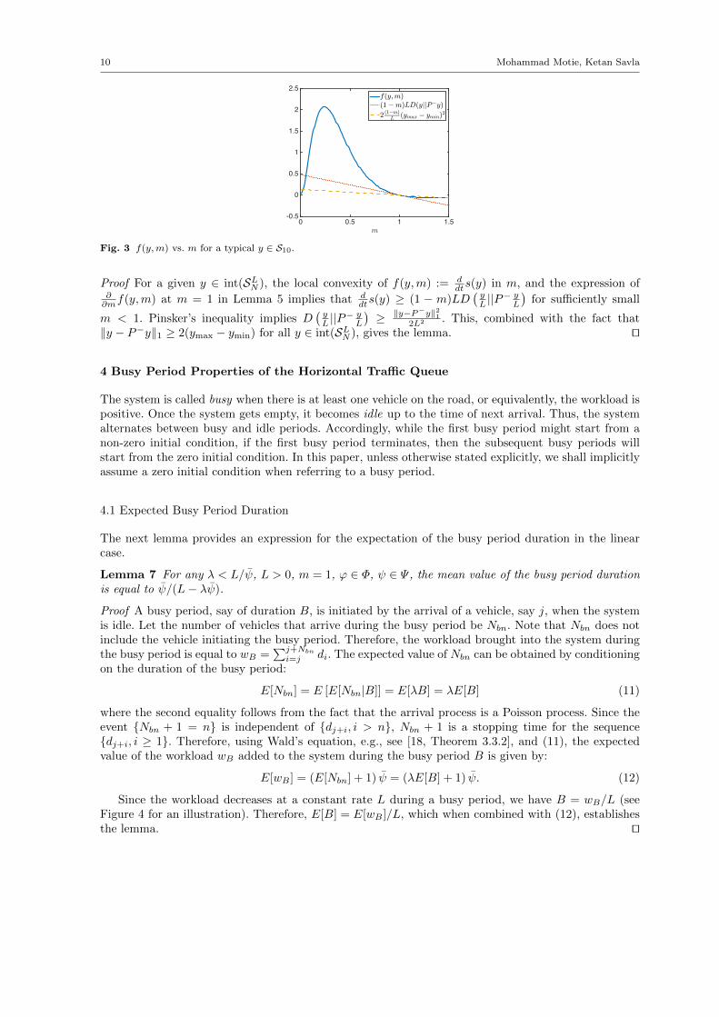
∂mf(y,m) in Lemma 5 at m = 1, and the fact thatf(y, 1) = 0 for all y, to develop a linear approximation in m of f(y,m) around m = 1. The followinglemma derives this approximation, as also suggested by Figure 3.
Lemma 6 For a given y ∈ int(SLN ), n ∈ N, L ∈ (0, e−2), there exists m(y) ∈ [0, 1) such that
d
dts(y) ≥ 2
(1−m)
L(ymax − ymin)
2, ∀m ∈ [m(y), 1]
10 Mohammad Motie, Ketan Savla
m0 0.5 1 1.5
-0.5
0
0.5
1
1.5
2
2.5f(y;m)(1!m)LD(yjjP!y)
2 (1!m)L (ymax ! ymin)
2
Fig. 3 f(y,m) vs. m for a typical y ∈ S10.
Proof For a given y ∈ int(SLN ), the local convexity of f(y,m) := ddts(y) in m, and the expression of
∂∂mf(y,m) at m = 1 in Lemma 5 implies that d
dts(y) ≥ (1 − m)LD(yL ||P
− yL
)for sufficiently small
m < 1. Pinsker’s inequality implies D(yL ||P
− yL
)≥ ‖y−P−y‖21
2L2 . This, combined with the fact that‖y − P−y‖1 ≥ 2(ymax − ymin) for all y ∈ int(SLN ), gives the lemma. ut
4 Busy Period Properties of the Horizontal Traffic Queue
The system is called busy when there is at least one vehicle on the road, or equivalently, the workload ispositive. Once the system gets empty, it becomes idle up to the time of next arrival. Thus, the systemalternates between busy and idle periods. Accordingly, while the first busy period might start from anon-zero initial condition, if the first busy period terminates, then the subsequent busy periods willstart from the zero initial condition. In this paper, unless otherwise stated explicitly, we shall implicitlyassume a zero initial condition when referring to a busy period.
4.1 Expected Busy Period Duration
The next lemma provides an expression for the expectation of the busy period duration in the linearcase.
Lemma 7 For any λ < L/ψ, L > 0, m = 1, ϕ ∈ Φ, ψ ∈ Ψ , the mean value of the busy period durationis equal to ψ/(L− λψ).
Proof A busy period, say of duration B, is initiated by the arrival of a vehicle, say j, when the systemis idle. Let the number of vehicles that arrive during the busy period be Nbn. Note that Nbn does notinclude the vehicle initiating the busy period. Therefore, the workload brought into the system duringthe busy period is equal to wB =
∑j+Nbn
i=j di. The expected value of Nbn can be obtained by conditioningon the duration of the busy period:
E[Nbn] = E [E[Nbn|B]] = E[λB] = λE[B] (11)
where the second equality follows from the fact that the arrival process is a Poisson process. Since theevent {Nbn + 1 = n} is independent of {dj+i, i > n}, Nbn + 1 is a stopping time for the sequence{dj+i, i ≥ 1}. Therefore, using Wald’s equation, e.g., see [18, Theorem 3.3.2], and (11), the expectedvalue of the workload wB added to the system during the busy period B is given by:
E[wB ] = (E[Nbn] + 1) ψ = (λE[B] + 1) ψ. (12)
Since the workload decreases at a constant rate L during a busy period, we have B = wB/L (seeFigure 4 for an illustration). Therefore, E[B] = E[wB ]/L, which when combined with (12), establishesthe lemma. ut

Service Rate, Busy Period & Throughput Analysis of a Horizontal Traffic Queue 11
1d
2d3d
4d
5d
Lddddd /)( 54321 ����
w
Fig. 4 (a) Queue length process and (b) workload process during a busy period.
Remark 3 Since the mean busy period duration is an upper bound on the mean waiting time, Lemma7 also gives an upper bound on the mean waiting time. One can then use Little’s law [13]1 to show thatthe mean queue length is upper bounded by λψ/(L− λψ).
Let I(t) :=∫ t0δ{w(s)=0}ds be the cumulative idle time up to time t. The following result characterizes
the long run proportion of the idle time in the linear case.
Proposition 1 For any λ < L/ψ, m = 1, L > 0, ϕ ∈ Φ,ψ ∈ Ψ , the long-run proportion of time inwhich HTQ is idle is given by the following:
limt→∞
I(t)
t= 1− λψ
L> 0 a.s.
Proof HTQ alternates between busy and idle periods. Let Z = I + B be the duration of a cycle thatcontains an idle period of length I followed by a busy period of length B. Idle period, I, has the samedistribution as inter-arrival times i.e. an exponential random variable with mean 1/λ, and the meanvalue of B is given in Lemma 7. Note that duration of cycles, Z, are i.i.d. random variables. Thus,the busy-idle profile of the system is an alternating renewal process where renewals correspond to themoments at which the system gets idle. Suppose the system earns reward at a rate of one per unit of timewhen it is idle (and thus the reward for a cycle equals the idle time of that cycle i.e. I). Then, the totalreward earned up to time t is equal to the total idle time in [0, t] (or I(t)), and by the result for renewalreward process (see [18], Theorem 3.6.1), with probability one, limt→∞ I(t)/t = E[I]/(E[B]+E[I]). ut
4.2 Busy Period Distribution
In this section, we compute the cumulative distribution function for the number of new arrivals duringa busy period for a HTQ with constant service rate, say p > 0. This could, e.g., correspond to (3) form = 1. However, our analysis in this section, is not restricted to this specific model, but applies to anyHTQ with constant service rate p. This cumulative distribution for the number of new arrivals duringa busy period, while of independent interest, will be used to derive lower bounds on the throughputin the super-linear case in Section 5.3. Our analysis is inspired by that of M/G/1 queue, e.g., see [18],where our consideration for non-zero initial condition appears to be novel.
1 Little’s law has previously been used in the context of processor sharing queues, e.g., in [1].
12 Mohammad Motie, Ketan Savla
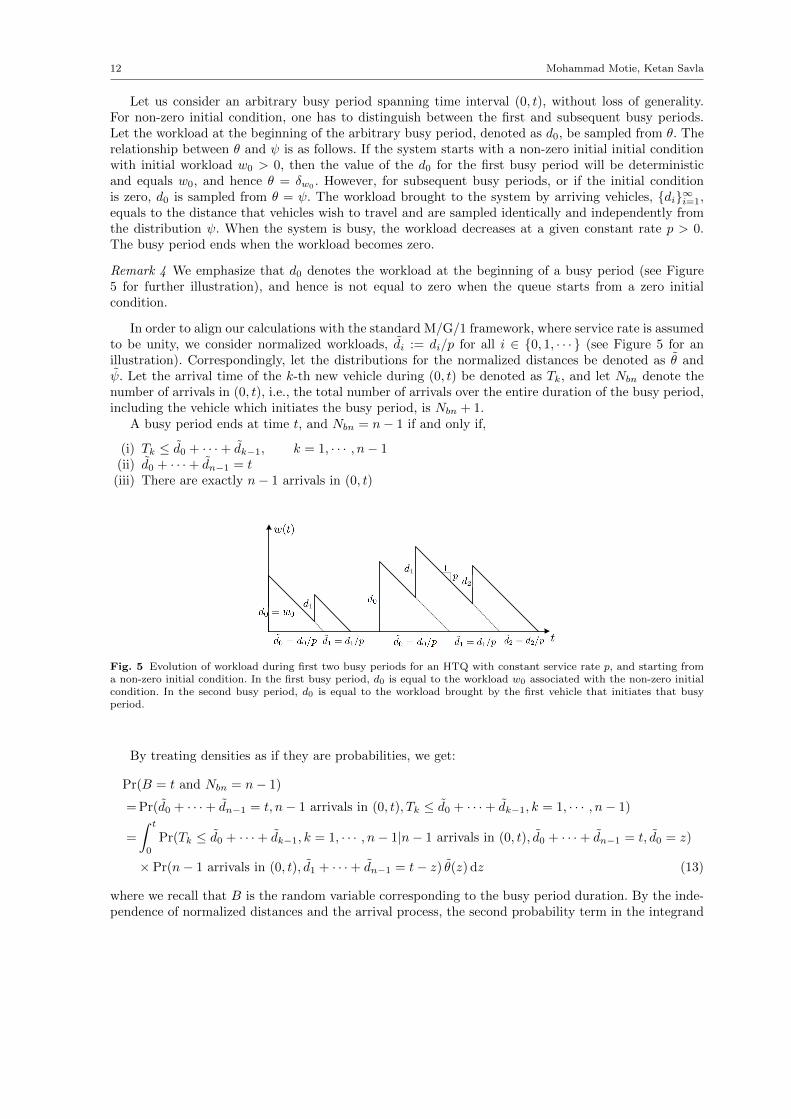
Let us consider an arbitrary busy period spanning time interval (0, t), without loss of generality.For non-zero initial condition, one has to distinguish between the first and subsequent busy periods.Let the workload at the beginning of the arbitrary busy period, denoted as d0, be sampled from θ. Therelationship between θ and ψ is as follows. If the system starts with a non-zero initial initial conditionwith initial workload w0 > 0, then the value of the d0 for the first busy period will be deterministicand equals w0, and hence θ = δw0 . However, for subsequent busy periods, or if the initial conditionis zero, d0 is sampled from θ = ψ. The workload brought to the system by arriving vehicles, {di}∞i=1,equals to the distance that vehicles wish to travel and are sampled identically and independently fromthe distribution ψ. When the system is busy, the workload decreases at a given constant rate p > 0.The busy period ends when the workload becomes zero.
Remark 4 We emphasize that d0 denotes the workload at the beginning of a busy period (see Figure5 for further illustration), and hence is not equal to zero when the queue starts from a zero initialcondition.
In order to align our calculations with the standard M/G/1 framework, where service rate is assumedto be unity, we consider normalized workloads, di := di/p for all i ∈ {0, 1, · · · } (see Figure 5 for anillustration). Correspondingly, let the distributions for the normalized distances be denoted as θ andψ. Let the arrival time of the k-th new vehicle during (0, t) be denoted as Tk, and let Nbn denote thenumber of arrivals in (0, t), i.e., the total number of arrivals over the entire duration of the busy period,including the vehicle which initiates the busy period, is Nbn + 1.
A busy period ends at time t, and Nbn = n− 1 if and only if,
(i) Tk ≤ d0 + · · ·+ dk−1, k = 1, · · · , n− 1(ii) d0 + · · ·+ dn−1 = t
(iii) There are exactly n− 1 arrivals in (0, t)
Fig. 5 Evolution of workload during first two busy periods for an HTQ with constant service rate p, and starting froma non-zero initial condition. In the first busy period, d0 is equal to the workload w0 associated with the non-zero initialcondition. In the second busy period, d0 is equal to the workload brought by the first vehicle that initiates that busyperiod.
By treating densities as if they are probabilities, we get:
Pr(B = t and Nbn = n− 1)
= Pr(d0 + · · ·+ dn−1 = t, n− 1 arrivals in (0, t), Tk ≤ d0 + · · ·+ dk−1, k = 1, · · · , n− 1)
=
∫ t
0
Pr(Tk ≤ d0 + · · ·+ dk−1, k = 1, · · · , n− 1|n− 1 arrivals in (0, t), d0 + · · ·+ dn−1 = t, d0 = z)
× Pr(n− 1 arrivals in (0, t), d1 + · · ·+ dn−1 = t− z) θ(z) dz (13)
where we recall that B is the random variable corresponding to the busy period duration. By the inde-pendence of normalized distances and the arrival process, the second probability term in the integrand
Service Rate, Busy Period & Throughput Analysis of a Horizontal Traffic Queue 13
in (13) can be expressed as
Pr(n− 1 arrivals in (0, t), d1 + · · ·+ dn−1 = t− z) = e−λt(λt)n−1
(n− 1)!ψn−1(t− z) (14)
where ψn is the n-fold convolution of ψ with itself.
In the first probability term in (13), it is given that the system receives n−1 arrivals in (0, t) and sincethe arrival process is a Poisson process, the ordered arrival times, {T1, T2, · · · , Tn−1}, are distributedas the ordered values of a set of n − 1 independent uniform (0, t) random variables {a1, a2, · · · , an−1}(see Theorem 2.3.1 in [18]). Thus,
Pr(Tk ≤ d0 + · · ·+ dk−1, k = 1, · · · , n− 1|n− 1 arrivals in (0, t), d0 + · · ·+ dn−1 = t, d0 = z)
= Pr(ak ≤ d0 + · · ·+ dk−1, k = 1, · · · , n− 1|d0 + · · ·+ dn−1 = t, d0 = z) (15)
By noting that t − U will also be a uniform (0, t) random variable whenever U is, it follows thata1, · · · , an−1 has the same joint distribution as t − an−1, · · · , t − a1. Thus, replacing ak with an−k fork ∈ {1, · · · , n− 1} in (15), we get
Pr(ak ≤ d0 + · · ·+ dk−1, k = 1, · · · , n− 1|d0 + · · ·+ dn−1 = t, d0 = z)
= Pr(t− an−k ≤ d0 + · · ·+ dk−1, k = 1, · · · , n− 1|d0 + · · ·+ dn−1 = t, d0 = z)
= Pr(t− an−k ≤ t− (dk + · · ·+ dn−1), k = 1, · · · , n− 1|d0 + · · ·+ dn−1 = t, d0 = z)
= Pr(an−k ≥ dk + · · ·+ dn−1, k = 1, · · · , n− 1|d0 + · · ·+ dn−1 = t, d0 = z)
= Pr(an−k ≥ dk + · · ·+ dn−1, k = 1, · · · , n− 1|d0 + · · ·+ dn−1 = t, d0 = z) =
{z/t z < t
0 otherwise
(16)
where the last equality follows from Lemma 14. If we let Hp(t, n, θ) := Pr{B ≤ t,Nbn = n − 1} whenthe service rate equals p, and d0 has distribution θ; then, by plugging (14) and (16) in (13), we get
d
dtHp(t, n, θ) = e−λt
(λt)n−1
t(n− 1)!
∫ t
0
zψn−1(t− z)θ(z)dz
By recalling the two special cases of interest to us: θ = δw0 for a given non-zero initial workload w0,and θ = ψ for zero initial condition, and using Lemma 13, we get that
Gp(t, n, θ) :=d
dtHp(t, n, θ) =
{e−λt (λt)
n−1w0
t(n−1)!p ψn−1(t− w0/p) θ = δw0
e−λt (λt)n−1
n! ψn(t) θ = ψ(17)
For r ∈ N, let Gr,p(t, n, θ) be the r-fold convolution of Gp(t, n, θ), defined in (17), with respect tot. In words, Gr,p(t, n, θ) is the probability that the number of new arrivals in each of (any) r busyperiods is equal to n− 1, and that the sum of durations of all the busy periods is equal to t. Similarly,for non-zero initial condition, let Gp1(θ1) ∗Gr−1,p2(θ2)(t, n) be the probability that the number of newarrivals in each of (any) r busy periods is equal to n− 1, and that the sum of durations of all the busyperiods is equal to t, when the constant service rate for the first busy period is p1 and is p2 for the restof the r − 1 busy periods.
14 Mohammad Motie, Ketan Savla
5 Throughput Analysis
5.1 Linear Case: m = 1
In this section, we provide an exact characterization of throughput for the linear case, i.e., when m = 1.Recall that, for m = 1, the service rate s(y) =
∑Ni=1 yi ≡ L is constant.
Proposition 2 For any L > 0, ϕ ∈ Φ, ψ ∈ Ψ , x0 ∈ [0, L]n0 , n0 ∈ N and :
λmax(L,m = 1, ϕ, ψ, x0, δ = 0) ≤ L/ψ .
Proof By contradiction, assume λmax > L/ψ. Let r(t) :=∑A(t)i=1 di be the workload added to the system
by the A(t) vehicles that arrive over [0, t]. Therefore,
w(t) = w0 + r(t)− L(t− I(t)) (18)
where w0 is the initial workload. The process {r(t), t ≥ 0} is a renewal reward process, where therenewals correspond to arrivals of vehicles and the rewards correspond to the distances {di}∞i=1 thatvehicles wish to travel in the system upon arrival before their departures. Inter-arrival times are expo-nential random variables with mean 1/λ, and the reward associated with each renewal is independentlyand identically sampled from ψ, whose mean is ψ. Therefore, e.g., [18, Theorem 3.6.1] implies that, withprobability one,
limt→∞
r(t)
t= λψ (19)
Thus, for all ε ∈(0, λψ − L
), there exists a t0 ≥ 0 such that, with probability one,
r(t)
t≥ λψ − ε/2 > L+ ε/2 ∀ t ≥ t0. (20)
Since w0 and I(t) are both non-negative, (18) implies that w(t) ≥ r(t)−Lt for all t ≥ 0. This combinedwith (20) implies that, with probability one, w(t) ≥ εt/2 for all t ≥ t0, and hence limt→∞ w(t) = +∞.This combined with (5) implies that, with probability one, limt→∞N(t) = +∞. ut
Theorem 1 For any L > 0, ϕ ∈ Φ, ψ ∈ Ψ , x0 ∈ [0, L]n0 , n0 ∈ N:
λmax(L,m = 1, ϕ, ψ, x0, δ = 1) = L/ψ .
Proof Assume that for some λ < L/ψ, there exists some initial condition (x0, n0) such that the queuelength grows unbounded with some positive probability. Since the workload brought by every vehicleis i.i.d., and the inter-arrival times are exponential, without loss of generality, we can assume that thequeue length never becomes zero. That is, the idle time satisfies I(t) ≡ 0. Moreover, (19) implies that,for every ε ∈
(0, L− λψ
), there exists t0 ≥ 0 such that, with probability one,
r(t)
t≤ λψ + ε/2 < L− ε/2 ∀t ≥ t0 (21)
Combining (18) with (21), and substituting I(t) ≡ 0, we get w(t) < w0 − εt/2, which impliesthat workload, and hence queue length, goes to zero in finite time after t0, leading to a contradiction.Combining this with the upper bound proven in Proposition 2 gives the result. ut
Remark 5 Theorem 1 implies that the throughput in the linear case is equal to the inverse of the timerequired to travel average total distance by a solitary vehicle in the system. In the linear case, thethroughput can be characterized with probability one, independent of the initial condition of the queue.
Service Rate, Busy Period & Throughput Analysis of a Horizontal Traffic Queue 15
5.2 Monotonicity of Throughput in m and x0
In this section, we show the following monotonicity property of λmax with respect to m for small valuesof L: for given x0 ∈ [0, L]n0 , n0 ∈ N, L ∈ (0, 1), ϕ ∈ Φ, and ψ ∈ Ψ , throughput is a monotonicallydecreasing function of m. For this section, we rewrite (2) in RN+ , i.e., without projecting onto [0, L]N .Specifically, let the vehicle coordinates be given by the solution of
xi = ymi , xi(0) = x0,i, i ∈ {1, . . . , N} (22)
Let X(t;x0,m) denote the solution to (22) at t starting from x0 at t = 0. We will compare X(t;x0,m)under different values of m and initial conditions x0, over an interval of the kind [0, τ), in betweenarrivals and departures. We recall the notation that, if x10 and x20 are vectors of different sizes, thenx10 ≤ x20 implies element-wise inequality only for components which are common to x10 and x20. InLemma 8 and Proposition 3, this common set of components corresponds to the set of vehicles commonbetween x10 and x20.
Lemma 8 For any L ∈ (0, 1], x10 ∈ Rn1+ , x20 ∈ Rn2
+ , n1, n2 ∈ N,
x10 ≤ x20, n2 ≤ n1, 0 < m2 ≤ m1 =⇒ X(t;x10,m1) ≤ X(t;x20,m2) ∀ t ∈ [0, τ)
Proof The proof is straightforward when n1 = n2. This is because, in this case, since yi ≤ L ≤ 1,m2 ≤ m1 implies ym2
i ≥ ym1i for all i ∈ {1, . . . , n1}. Using this with Lemmas 10 and 11 gives the result.
In order to prove the result for n2 < n1, we show that X(t;x10,m1) ≤ X(t;x20,m1) ≤ X(t;x20,m2).Note that the second inequality follows from the previous case. Therefore, it remains to prove the firstinequality. Let (i1, . . . , in2) be the set of indices of n2 vehicles such that 0 ≤ x20,i1 ≤ . . . ≤ x20,in2
≤ L.
Similarly, let (i1, i1+1, . . . , i2, i2+1, . . .) be the indices of n1 vehicles in the order of increasing coordinatesin x10. Our assumption on the initial condition implies that x10,ik ≤ x20,ik for all k ∈ {1, . . . , n2}. For
brevity, let x1(t) ≡ X(t;x10,m1), and x2(t) ≡ X(t;x20,m1). It is easy to check that, for all t ∈ [0, τ), andall k ∈ {1, . . . , n2},
x1ik =(x1ik+1 − x1ik
)m1 ≤(x1ik+1
− x1ik)m1
(23)
Let t ∈ [0, τ) be the first time instant when x1ik(t) = x2ik(t) for some k ∈ {1, . . . , n2}. Then, recalling
x1ik+1(t) ≤ x2ik+1
(t), (23) implies that x1ik(t) ≤(x2ik+1
− x2ik)m1
= x2ik(t). The result then follows from
Lemma 10. ut
Lemma 8 is used to establish monotonicity of throughput as follows.
Proposition 3 For any L ∈ (0, 1], ϕ ∈ Φ, ψ ∈ Ψ , δ ∈ (0, 1), x10 ∈ [0, L]n1 , x20 ∈ [0, L]n2 , n1, n2 ∈ N:
x10 ≤ x20, n2 ≤ n1, 0 < m2 ≤ m1 =⇒ λmax(L,m1, ϕ, ψ, x10, δ) ≤ λmax(L,m2, ϕ, ψ, x
20, δ)
Proof For brevity in notation, we refer to the queue corresponding to m1, and initial condition x10 asHTQ-S. We refer to the other queue as HTQ-F. Let λ, ϕ and ψ common to HTQ-S and HTQ-F begiven. Let x1(t) ≡ X(t;x10,m1) and x2(t) ≡ X(t;x20,m2), and let Ns(t) and Nf (t) be the queue lengthsin the two queues at time t. It suffices to show that Ns(t) ≥ Nf (t) for a given realization of arrivaltimes, arrival locations, and travel distances. In particular, this also implies that the departure locationsare also the same for every vehicle, including the vehicles present at t = 0, in both the queues.
Indeed, it is sufficient to show that x1(τ) ≤ x2(τ) and Ns(τ) ≥ Nf (τ) where τ is the time of firstarrival or departure from either HTQ-S or HTQ-F. Accordingly, we consider two cases, correspondingto whether τ corresponds to arrival or departure.
Since x1(t) ≤ x2(t) for all t ∈ [0, τ) from Lemma 8, and the departure locations of all the vehiclesin HTQ-S and HTQ-F are identical, the first departure from HTQ-S can not happen before the firstdeparture in HTQ-F. Therefore, Ns(τ) ≥ Nf (τ). Since x1(τ−) ≤ x2(τ−), and x2(τ) is a subset ofx2(τ−), we also have x1(τ) ≤ x2(τ).
16 Mohammad Motie, Ketan Savla
When τ corresponds to the time of the first arrival, since the arrivals happen at the same location inHTQ-S and HTQ-F, and since x1(τ−) ≤ x2(τ−), rearrangement of the indices of the vehicles to includethe new arrival at t = τ implies that x1(τ) ≤ x2(τ). Moreover, since Ns(τ
−) ≥ Nf (τ−), and the arrivalshappen simultaneously in both HTQ-S and HTQ-F, we have Ns(τ) ≤ Nf (τ). ut
Remark 6 Proposition 3 establishes monotonicity of throughput only for L ∈ (0, 1]. This is consistentwith our simulation studies, e.g., as reported in Figure 2, according to which, the throughput is non-monotonic for large L.
For the analysis of the linear car following model, we exploited the fact that the total service rate ofthe system is constant. However, for the nonlinear model, i.e., m 6= 1, the total service rate dependson the number and relative locations of vehicles. The state dependent service rate of nonlinear modelsmakes the throughput analysis much more complex. In the next section, we find probabilistic bound onthe throughput in the super-linear case.
5.3 Throughput Bounds for the Super-linear Case from Busy Period Calculations
In this section, we derive lower bound on the throughput for the super-linear case. The next resultcomputes a bound on the probability that the queue length of the HTQ satisfies a given upper boundover a given time interval, using the probability distribution functions from (17). In Propositions 4 and5, for the sake of clarity, we add explicit dependence on λ to this probability distribution function.
Proposition 4 For any m > 1, M ∈ N, L > 0, λ > 0, ϕ ∈ Φ, ψ ∈ Ψ , and zero initial condition x0 = 0,the probability that the queue length is upper bounded by M over a given time interval [0, T ] satisfiesthe following bound:
Pr(N(t) ≤M ∀t ∈ [0, T ]
)≥ sup
r∈N
M∑n=1
∫ ∞T
Gr,LmM1−m(t, n, ψ, λ) dt (24)
Proof Let us denote the current queueing system as HTQ-f. We shall compare queue lengths betweenHTQ-f and a slower queueing system HTQ-s, which starts from the same (zero) initial condition, andexperiences the same realizations of arrival times, locations and travel distances. Let every incomingvehicle into HTQ-s and HTQ-f be tagged with a unique identifier. At time t, let J (t) be the set ofidentifiers of vehicles present both in HTQ-s and HTQ-f, Js/f (t) be the set of identifiers of vehicles
present only in HTQ-s, and Jf/s(t) be the set of identifiers of vehicles present only in HTQ-f. Let vfidenote the speed of the vehicle in HTQ-f with identifier i ∈ J (t) ∪ Jf/s(t), as determined by the car-following behavior underlying (2). The vehicle speeds in HTQ-s are not governed by the car followingbehavior, but are rather related to the speeds of vehicles in HTQ-f as:
vsi (t) =
vfi (t)
p
vf (t)
|J (t)||J (t)|+ |Js/f (t)|
i ∈ J (t)
p
|J (t)|+ |Js/f (t)|i ∈ Js/f (t)
(25)
where vf (t) :=∑i∈J (t) v
fi (t) is the sum of speeds of vehicles in HTQ-f that are also present in HTQ-s
at time t, and p is a parameter to be specified. Indeed, note that∑i∈J (t)∪Js/f (t)
vsi (t) ≡ p, i.e., p is the
(constant) service rate of HTQ-s.Consider a realization where the number of arrivals into HTQ-s with p = LmM1−m during any busy
period overlapping with [0, T ] does not exceed M . We refer to such a realization as event in the restof the proof. Since the maximum queue length during a busy period is trivially upper bounded by thenumber of arrivals during that busy period, conditioned on the event, we have
Ns(t) ≤M, t ∈ [0, T ] (26)
Service Rate, Busy Period & Throughput Analysis of a Horizontal Traffic Queue 17
Consider the union of departure epochs from HTQ-s and HTQ-f in [0, T ]: 0 = τ0 ≤ τ1 ≤ . . .. IfJf/s(τk) = ∅ for some k ≥ 0, then Jf/s(t) = ∅ for all t ∈ (τk, τk+1). Hence, the service rate for HTQ-f
over the interval (τk, τk+1) is vf (t), which, conditioned on the event, is lower bounded by LmM1−m = pby Lemma 2. Therefore, p/vf (t) ≤ 1 over (τk, τk+1), and hence (25) implies that all the vehicles withidentifiers in Jf will travel slower in HTQ-s in comparison to HTQ-f. In particular, this implies thatJf/s(τk+1) = ∅. This, combined with the fact that Jf/s(τ0) = ∅ (both the queues start from the sameinitial condition), we get that, conditioned on the event, Js/f (t) ≡ ∅, and hence N(t) ≤ Ns(t) over[0, T ]. Combining this with (26) gives that, conditioned on the event, N(t) ≤M over [0, T ].
We now compute the probability of the occurrence of the event using busy period calculations fromSection 4.2. The event can be categorized by the maximum number of busy periods, say r ∈ N, that over-lap with [0, T ], i.e., the r-th busy period ends after time T (and each of these busy periods has at mostM arrivals). Since these busy periods are interlaced with idle periods, the probability of the r-th busyperiod ending after time T is lower bounded by the probability that the sum of the durations of r busyperiods is at least T . (17) implies that the latter quantity is equal to
∑Mn=1
∫∞TGr,LmM1−m(t, n, ψ, λ) dt.
The proposition then follows by noting that this is true for any r ∈ N. ut
Remark 7 In the proof of Proposition 4, when deriving probabilistic upper bound on the queue lengthover a given time horizon [0, T ], we neglected the idle periods in [0, T ]. This introduces conservatism inthe bound on the right hand side of (24). Since the idle period durations are distributed independentlyand identically according to an exponential random variable (since the arrival process is Poisson), onecould incorporate them into (24) by taking convolution of G with idle period distributions. Our choicefor not doing so here is to ensure conciseness in the presentation of bounds in (24). The resultingconservatism is also present in Proposition 5, and carries over to Theorems 2 and 3, as well as to thecorresponding simulations reported in Figures 7, 8 and 9.
The next result generalizes Proposition 4 for non-zero initial condition. Note that the non-zero initialcondition only affects the first busy period; all subsequent busy periods will necessarily start from withzero initial condition.
Proposition 5 For any m > 1, M ∈ N, L > 0, λ > 0, ϕ ∈ Φ, ψ ∈ Ψ , initial condition x0 ∈ [0, L]n0 ,n0 ∈ N, with associated workload w0 > 0, the probability that the queue length is upper bounded byM + n0 over a given time interval [0, T ] satisfies the following:
Pr(N(t) ≤M + n0 ∀t ∈ [0, T ]
)≥ sup
r∈N
M∑n=1
∫ ∞T
GLm(M+n0)1−m(δw0) ∗Gr−1,LmM1−m(ψ)(t, n, λ) dt
Proof The proof is similar to the proof of Proposition 4; however, since we consider M number of newarrivals in each of the busy periods, the event of interest is when the queue length in HTQ-s doesnot exceed M + n0 and M in the first and subsequent busy periods, respectively, while operating withconstant service rates Lm(M + n0)1−m and LmM1−m, respectively. ut
We shall use Propositions 4 and 5 to establish probabilistic lower bound for a finite time horizonversion of the throughput defined in Definition 1: for T > 0, let
λmax(L,m,ϕ, ψ, x0, δ, T ) := sup {λ ≥ 0 : Pr (N(t;L,m, λ, ϕ, ψ, x0) < +∞, ∀t ∈ [0, T ]) ≥ 1− δ} .
Theorem 2 For L > 0, m > 1, ϕ ∈ Φ, ψ ∈ Ψ , δ ∈ (0, 1), T > 0, zero initial condition x0 = 0,
λmax(L,m,ϕ, ψ, x0, δ, T ) ≥ supM∈N
sup{λ ≥ 0
∣∣∣ supr∈N
M∑n=1
∫ ∞T
Gr,LmM1−m(t, n, ψ, λ) dt ≥ 1− δ}
(27)
Proof Follows from Proposition 4. ut
18 Mohammad Motie, Ketan Savla
Theorem 3 For L > 0, m > 1, ϕ ∈ Φ, ψ ∈ Ψ , δ ∈ (0, 1), T > 0, initial condition x0 ∈ [0, L]n0 , n0 ∈ N,with associated workload w0 > 0,
λmax(L,m,ϕ, ψ, x0, δ, T )
≥ supM∈N
sup{λ > 0
∣∣∣ supr∈N
M∑n=1
∫ ∞T
GLm(M+n0)1−m(δw0) ∗Gr−1,LmM1−m(ψ)(t, n, λ) ≥ 1− δ}
Proof Follows from Proposition 5. ut
Remark 8 In Theorems 2 and 3, we implicitly assume the rather standard convention that supremumover an empty set is zero.
5.4 Throughput Bounds under Batch Release Control Policy
In this section, we consider a time-perturbed version of the arrival process. For a given realization ofarrival times, {t1, t2, · · · }, consider a perturbation map t′i ≡ t′i(t1, . . . , ti) satisfying t′i ≥ ti for all i, whichprescribes the perturbed arrival times. The magnitude of perturbation is defined as η := E (t′i − ti),where the expectation is with respect to the Poisson process with rate λ that generates the arrivaltimes.
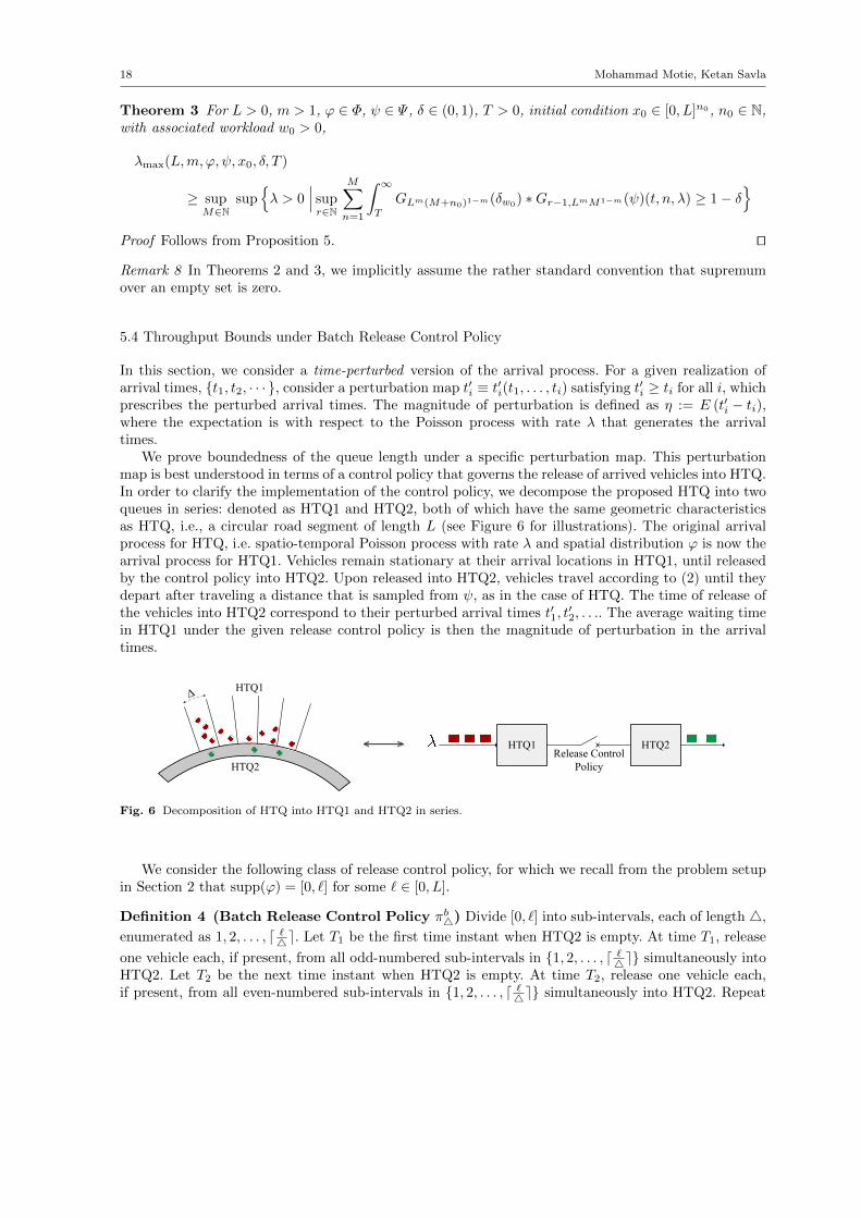
We prove boundedness of the queue length under a specific perturbation map. This perturbationmap is best understood in terms of a control policy that governs the release of arrived vehicles into HTQ.In order to clarify the implementation of the control policy, we decompose the proposed HTQ into twoqueues in series: denoted as HTQ1 and HTQ2, both of which have the same geometric characteristicsas HTQ, i.e., a circular road segment of length L (see Figure 6 for illustrations). The original arrivalprocess for HTQ, i.e. spatio-temporal Poisson process with rate λ and spatial distribution ϕ is now thearrival process for HTQ1. Vehicles remain stationary at their arrival locations in HTQ1, until releasedby the control policy into HTQ2. Upon released into HTQ2, vehicles travel according to (2) until theydepart after traveling a distance that is sampled from ψ, as in the case of HTQ. The time of release ofthe vehicles into HTQ2 correspond to their perturbed arrival times t′1, t
′2, . . .. The average waiting time
in HTQ1 under the given release control policy is then the magnitude of perturbation in the arrivaltimes.
HTQ1 Release Control Policy
HTQ2HTQ1
HTQ2
(a) (b)
1x
2x
3x
1y 2y
3y0 L
' HTQ1
HTQ2
HTQ1Release Control
Policy
HTQ2
Fig. 6 Decomposition of HTQ into HTQ1 and HTQ2 in series.
We consider the following class of release control policy, for which we recall from the problem setupin Section 2 that supp(ϕ) = [0, `] for some ` ∈ [0, L].
Definition 4 (Batch Release Control Policy πb4) Divide [0, `] into sub-intervals, each of length 4,
enumerated as 1, 2, . . . , d `4e. Let T1 be the first time instant when HTQ2 is empty. At time T1, release
one vehicle each, if present, from all odd-numbered sub-intervals in {1, 2, . . . , d `4e} simultaneously intoHTQ2. Let T2 be the next time instant when HTQ2 is empty. At time T2, release one vehicle each,if present, from all even-numbered sub-intervals in {1, 2, . . . , d `4e} simultaneously into HTQ2. Repeat
Service Rate, Busy Period & Throughput Analysis of a Horizontal Traffic Queue 19
this process of alternating between releasing one vehicle each from odd and even-numbered sub-intervalsevery time that HTQ2 is empty.
Remark 9 1. Under πb4, when vehicles are released into HTQ2, the inter-vehicle distances in the frontand rear of each vehicle being released is at least equal to 4.
2. The order in which vehicles are released into HTQ2 from HTQ1 under πb4 may not be the same asthe order of arrivals into HTQ1.
In the next two sub-sections, we analyze the performance of the batch release control policy forsub-linear and super-linear cases.
5.4.1 The Sub-linear Case
In this section, we derive a lower bound on throughput when m ∈ (0, 1). We first derive a trivial lowerbound in Proposition 6 implied by Lemma 4 and Remark 2. Next, we improve this lower bound inTheorem 4 under a under a batch release control policy, πb4.
Proposition 6 For any L > 0, m ∈ (0, 1), ϕ ∈ Φ, ψ ∈ Ψ , x0 ∈ [0, L]n0 , n0 ∈ N:
λmax(L,m,ϕ, ψ, x0, δ = 0) ≥ Lm/ψ
Proof Remark 2 implies that, for m ∈ (0, 1), the service rate does not decrease due to arrivals. Therefore,a simple lower bound on the service rate for any state is the service rate when there is only one vehicle inthe system, i.e., Lm. Therefore, the workload process is upper bounded as w(t) = w0+r(t)−
∫ t0s(z)dz ≤
w0 + r(t) − Lm(t − I(t)), ∀t ≥ 0, where r(t) and I(t) denote the renewal reward and the idle timeprocesses, respectively, as introduced in the proof of Proposition 2. Similar to the proof of Proposition2, it can be shown that, if λ < Lm/ψ, then the workload, and hence the queue length, goes to zero infinite time with probability one. ut
Next, we establish better throughput guarantees than Proposition 6, under a batch release controlpolicy, πb4. The next result characterizes the time interval between release of successive batches into
HTQ2 under πb4.
Lemma 9 For given λ > 0, 4 > 0, ϕ ∈ Φ, ψ ∈ Ψ with supp(ψ) = [0, R], R > 0, m ∈ (0, 1),x0 ∈ [0, L]n0 , L > 0, n0 ∈ N, let T1, T2, . . . denote the random variables corresponding to time ofsuccessive batch releases into HTQ2 under πb4. Then, T1 ≤ n0R
Lm , Ti+1 − Ti ≤ R/4m for all i ≥ 1, andymin(t) ≥ 4 for all t ≥ T1.
Proof Since the maximum distance to be traveled by every vehicle is upper bounded by R, the initialworkload satisfies w0 ≤ n0R. Since the minimum service rate for m ∈ (0, 1) is Lm (see proof ofProposition 6), with no new arrivals, it takes at most w0/L
m = n0R/Lm amount of time for the system
to become empty. This establishes the bound on T1.Lemma 1 implies that, under πb4, the minimum inter-vehicle distance in HTQ2 is at least 4 after
T1. This implies that ymin(t) ≥ 4 for all t ≥ T1, and hence the minimum speed of every vehicle inHTQ2 is at least 4m after T1. Since the maximum distance to be traveled by every vehicle is R, thisimplies that the time between release of a vehicle into HTQ2 and its departure is upper bounded byR/4m, which in turn is also an upper bound on the time required by all the vehicles released in onebatch to depart from the system. ut
Let N1(t) and N2(t) denote the queue lengths in HTQ1 and HTQ2, respectively, at time t. Lemma 9implies that, for every4 > 0, N2(t) is upper bounded for all t ≥ T1. The next result identifies conditionsunder which N1(t) is upper bounded.
For F > 0, let ΦF :={ϕ ∈ Φ | supx∈[0,`] ϕ(x) ≤ F
}. For subsequent analysis, we now derive an
upper bound on the load factor, i.e., the ratio of the arrival and departure rates, associated with a
20 Mohammad Motie, Ketan Savla
typical sub-queue of HTQ1 among {1, 2, . . . , d `4e}. It is easy to see that, for every ϕ ∈ ΦF , F > 0,the arrival process into every sub-queue is Poisson with arrival rate upper bounded by λF4. Lemma 9implies that the departure rate is at least 4m/2R. Therefore, the load factor for every sub-queue isupper bounded as
ρ ≤ 2RλF44m
= 2RλF41−m (28)
In particular, if
4 < 4∗(λ) := (2RλF )− 1
1−m , (29)
then ρ < 1. It should be noted that for n0 < +∞, by Lemma 9, T1 < +∞. The service rate is zeroduring [0, T1]; however, since T1 is finite, this does not affect the computation of load factor.
Proposition 7 For any λ > 0, ϕ ∈ ΦF , F > 0, ψ ∈ Ψ with supp(ψ) = [0, R], R > 0, m ∈ (0, 1),x0 ∈ [0, L]n0 , L > 0, n0 ∈ N, for sufficiently small 4, N1(t) is bounded for all t ≥ 0 under πb4, almostsurely.
Proof By contradiction, assume that N1(t) grows unbounded. This implies that there exists at leastone sub-queue, say j ∈ {1, 2, . . . , d `4e}, such that its queue length, say N1,j(t), grows unbounded. In
particular, this implies that there exists t0 ≥ T1 such that N1,j(t) ≥ 2 for all t ≥ t0. Therefore, for allt ≥ t0, the ratio of arrival rate to departure rate for the j-th sub-queue is given by (28), which is adecreasing function of 4, and hence becomes strictly less than one for sufficiently small 4. A simpleapplication of the law of large numbers then implies that, almost surely, N1,j(t) = 0 for some finitetime, leading to a contradiction. ut
The following result gives an estimate of the mean waiting time in a typical sub-queue in HTQ1under the πb4 policy.
Proposition 8 For ϕ ∈ ΦF , F > 0, ψ ∈ Ψ , m ∈ (0, 1), there exists a sufficiently small 4 such thatthe average waiting time in HTQ1 under πb4 is upper bounded as:
W ≤ R(2RλF )m
1−m
(2
mm
1−m+
m
mm
1−m −m1
1−m
). (30)
Proof It is easy to see that the desired waiting time corresponds to the system time of an M/D/1queue with load factor given by (28) along with the arrival and departure rates leading to (28). Notethat, by Lemma 9, for finite n0, the value of T1 is finite and does not affect the average waiting time.Therefore, using standard expressions for M/D/1 queue [13], we get that the waiting time in HTQ1 isupper bounded as follows for ρ < 1:
W ≤ 2R
4m+
R
4mρ
1− ρ≤ 2R
4m+
R
4m1
1− ρ
≤ 2R
4m+
R
4m − 2RλF4(31)
It is easy to check that the minimum of the second term in (31) over(0,4∗(λ)
)occurs at 4 =(
m2RλF
) 11−m . Substitution in the right hand side of the first inequality in (31) gives the result. ut
Remark 10 (30) implies that, for every R > 0, F > 0, λ > 0, we have W → 2R as m→ 0+.
We extend the notation introduced in (4) to λmax(L,m,ϕ, ψ, x0, δ, η) to also show the dependenceon maximum allowable perturbation η. This is not to be confused with the notation for λmax used inTheorems 2 and 3, where we used the notion of throughput over finite time horizons. We choose to usethe same notations to maintain brevity.
In order to state the next result, for given R > 0, F > 0, m ∈ (0, 1) and η ≥ 0, let W (m,F,R, η) bethe value of λ for which the right hand side of (30) is equal to η, if such a λ exists and is at least Lm/ψ,and let it be equal to Lm/ψ, otherwise. The lower bound of Lm/ψ in the definition of W is inspired byProposition 6. The next result formally states W as a lower bound on λmax.
Service Rate, Busy Period & Throughput Analysis of a Horizontal Traffic Queue 21
Theorem 4 For any ϕ ∈ ΦF , F > 0, ψ ∈ Ψ with supp(ψ) = [0, R], R > 0, m ∈ (0, 1), x0 ∈ [0, L]n0 ,n0 ∈ N, L > 0, and maximum permissible perturbation η ≥ 0,
λmax(L,m,ϕ, ψ, x0, δ = 0, η) ≥ W (m,F,R, η)
In particular, if η > 2R, then λmax(L,m,ϕ, ψ, x0, δ = 0, η)→ +∞ as m→ 0+.
Proof Consider any λ ≤ W (m,F,R, η), and 4 ≤(
m2RλF
) 11−m . Under policy πb4, Lemma 9 and Propo-
sition 7 imply that, for finite n0, N2(t) and N1(t) remain bounded for all times, with probability one.Also, for λ = W (m,F,R, η), by Proposition 8 and the definition of W (m,F,R, η), the introduced per-turbation remains upper bounded by η. Since the right hand side of (30) is monotonically increasingin λ, perturbations remain bounded by η for all λ ≤ W (m,F,R, η). In particular, by Remark 10, wehave W → 2R as m→ 0+. In other words, as m→ 0+, the magnitude of the introduced perturbationbecomes independent of λ. Therefore, when η > 2R, and m → 0+ throughput can grow unboundedwhile perturbation and queue length remains bounded. ut
Remark 11 We emphasize that the only feature required in a batch release control policy is that, at themoment of release, the front and rear distances for the vehicles being released should be greater than 4.The requirement of the policy in Definition 4 for the road to be empty at the moment of release makesthe control policy conservative, and hence affects the maximum permissible perturbation. In fact, forspecial spatial distributions, e.g., when ϕ is a Dirac delta function and the support of ψ is [0, L−4]),one can relax the conservatism to guarantee unbounded throughput for arbitrarily small permissibleperturbation.
5.4.2 The Super-linear Case
In this section, we study the throughput for the super-linear case under perturbed arrival process witha maximum permissible perturbation of η. For this purpose, we consider the batch release control policyπb4, defined in Definition 4, for our analysis. Time intervals between release of successive batches, under
πb4, are characterized the same as Lemma 9. However, in the super linear case, by Lemma 2, the initial
minimum service rate is Lmn1−m0 . Therefore, the time of first release is bounded as T1 < nm0 R/Lm.
Moreover, similar to the proof of Lemma 9, it can be shown that ymin(t) ≥ 4 for all t ≥ T1.During [0, T1], the service rate of all sub-queues remain zero; however, when n0 < +∞, T1 is finite
and for the computation of load factor this time interval can be neglected. Therefore, the load factorfor each sub-queue will be the same as the sub-linear case (28). In this case, however, in order to haveρ < 1, we get the counterpart of (29) as:
4 > 4∗(λ). (32)
It should be noted that since the batch release control policy iteratively releases from odd and evensub-queues, we need at least two sub-queues to be able to implement this policy. As a result, 4 cannotbe arbitrary large and 4 < `/2. This constraint gives the following bound on the admissible throughputunder this policy
λ < λ∗ := (`/2)m−1/2RF (33)
The following result shows that for the above range of throughput, the queue length in HTQ1, N1(t),remains bounded at all times.
Proposition 9 For any λ < λ∗, 4 ∈(4∗(λ), `/2
], ϕ ∈ ΦF , F > 0, ψ ∈ Ψ with supp(ψ) = [0, R],
R > 0, m > 1, x0 ∈ [0, L]n0 , L > 0, n0 ∈ N, N1(t) is bounded for all t ≥ 0 under πb4, almost surely.
Proof The proof is similar to proof of Proposition 7. In particular, by (32) and (33), one can show thatload factor (28) remains strictly smaller than one. This implies that no sub-queue in HTQ1 can growunbounded, and N1(t) remains bounded for all times, with probability one. ut

22 Mohammad Motie, Ketan Savla
m1.1 1.2 1.3 1.4 1.5 1.6 1.7 1.8 1.9 2
λmax
0
0.1
0.2
0.3
0.4
0.5
0.6
0.7
0.8Estimate from Theorem 2, T = 500Estimate from Theorem 2, T = 20Lower Range of Numerical EstimateUpper Range of Numerical Estimate
(a)
m1.1 1.2 1.3 1.4 1.5 1.6 1.7 1.8 1.9 2
λmax
0
0.2
0.4
0.6
0.8
1
1.2
1.4
1.6
1.8Estimate from Theorem 2, T = 500Estimate from Theorem 2, T = 20Lower Range Numerical EstimateUpper Range Numerical Estimate
(b)
Fig. 7 Comparison between theoretical estimates of throughput from Theorem 2, and range of numerical estimates fromsimulations, for zero initial condition. The parameters used for this case are: L = 1, δ = 0.1, and (a) ϕ = δ0, ψ = δL, (b)ϕ = U[0,L], ψ = U[0,L].
Proposition 10 For any λ < λ∗, ϕ ∈ ΦF , F > 0, ψ ∈ Ψ , m > 1, the average waiting time in HTQ1under πb4 for 4 = `/2 is upper bounded as:
W ≤ 2R
(`/2)m+
R
(`/2)m2RλF (`/2)1−m
1− 2RλF (`/2)1−m(34)
Proof The proof is very similar to the proof of Proposition 8. Thus, we get the following bounds:
W ≤ 2R
4m+
R
4mρ
1− ρ≤ 2R
4m+
R
4m2RλF41−m
1− 2RλF41−m
The right hand side of the above inequality is a decreasing function of 4; therefore, 4 = `/2 minimizesit, and gives (34). ut
Let W (m,F,R, η) be the value of λ for which the right hand side of (34) is equal to η, if sucha λ ≤ λ∗ exists, and let it be equal to λ∗ otherwise. Note that since the right hand side of (34) ismonotonically increasing in λ, for all λ ≤ W (m,F,R, η) the introduced perturbation remains upperbounded by η.
Theorem 5 For any ϕ ∈ ΦF , F > 0, ψ ∈ Ψ with supp(ψ) = [0, R], R > 0, m > 1, x0 ∈ [0, L]n0 ,n0 ∈ N, L > 0, and maximum permissible perturbation η ≥ 0,
λmax(L,m,ϕ, ψ, x0, δ = 0, η) ≥ W (m,F,R, η).
Proof For any λ < W (m,F,R, η), under πb4, Lemma 9 and Proposition 9 imply that, for finite n0,N2(t) and N1(t) remain bounded for all times, with probability one. Also, by Proposition 10 and thedefinition of W (m,F,R, η), the introduced perturbation remains upper bounded by η. ut
6 Simulations
In this section, we present simulation results on throughput analysis, and compare with our theoreticalresults from previous sections.
Figures 7, 8 and 9 show comparison between the lower bound on throughput over finite time horizons,as given by Theorems 2 and 3, and the corresponding numerical estimates from simulations. Figures 7and 8 are for zero initial condition, and Figure 9 is for non-zero initial condition.
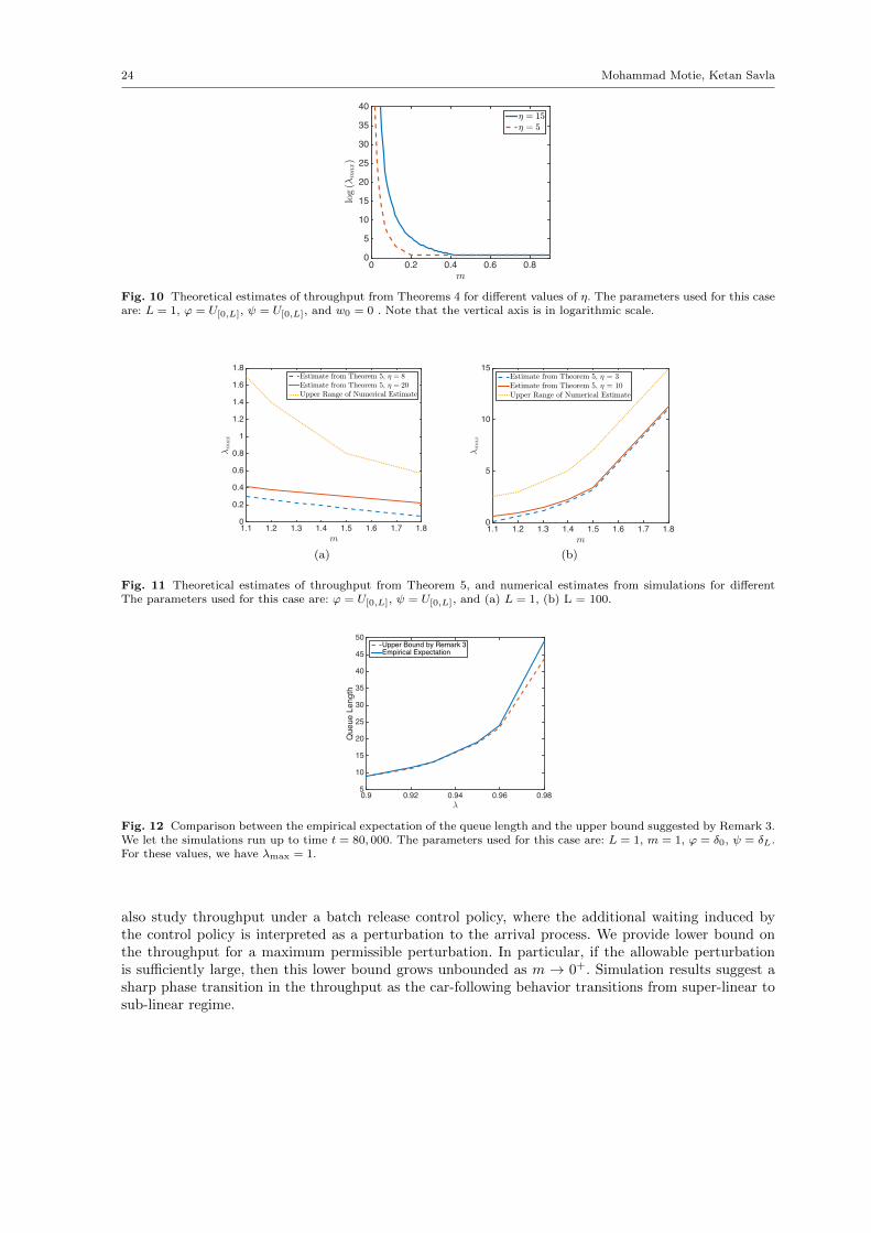
Figures 10 and 11 show comparison between the lower bound on throughput as given by the bacthrelease control policy, as per Theorems 4 and 5, respectively, under a couple of representative values
Service Rate, Busy Period & Throughput Analysis of a Horizontal Traffic Queue 23
m1.1 1.2 1.3 1.4 1.5 1.6 1.7 1.8
λmax
0
1
2
3
4
5
6
7Estimate from Theorem 2Upper Range of Numerical Estimate
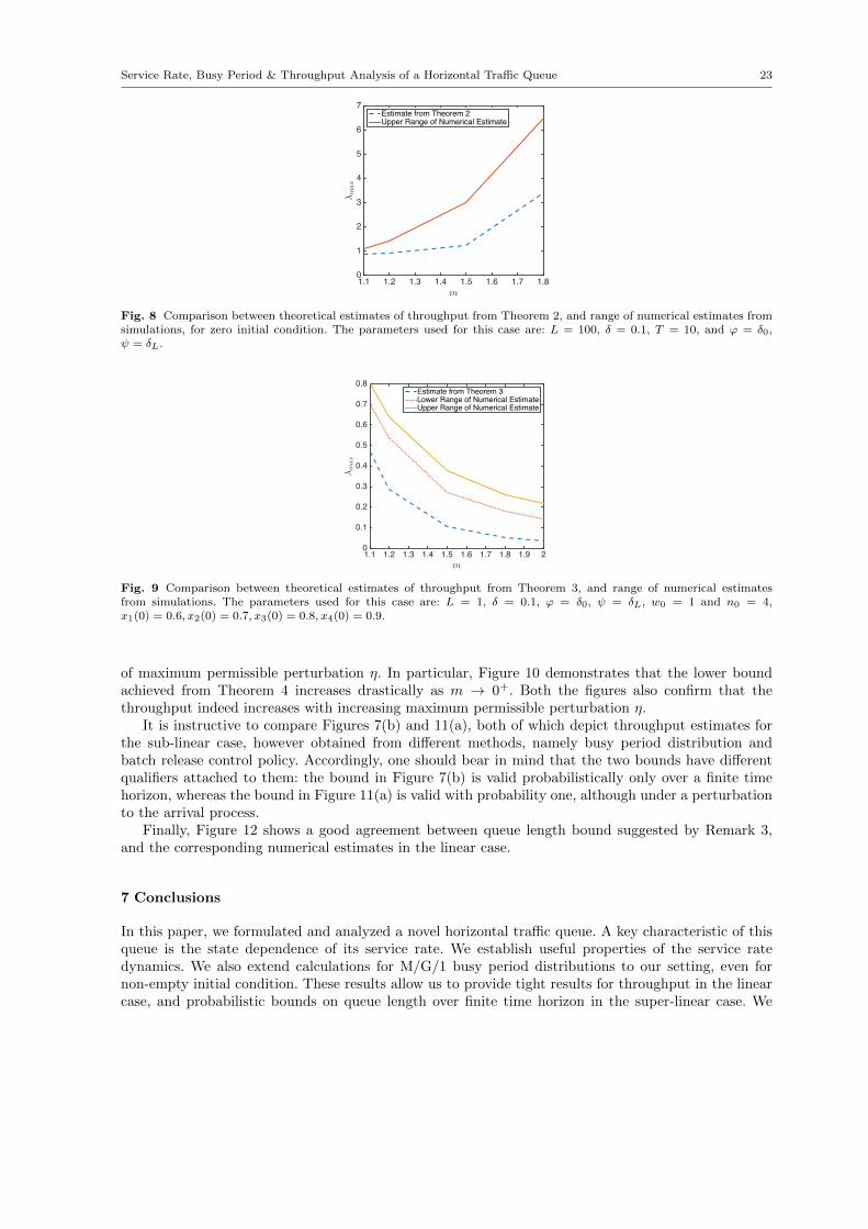
Fig. 8 Comparison between theoretical estimates of throughput from Theorem 2, and range of numerical estimates fromsimulations, for zero initial condition. The parameters used for this case are: L = 100, δ = 0.1, T = 10, and ϕ = δ0,ψ = δL.
m1.1 1.2 1.3 1.4 1.5 1.6 1.7 1.8 1.9 2
λmax
0
0.1
0.2
0.3
0.4
0.5
0.6
0.7
0.8Estimate from Theorem 3Lower Range of Numerical EstimateUpper Range of Numerical Estimate
Fig. 9 Comparison between theoretical estimates of throughput from Theorem 3, and range of numerical estimatesfrom simulations. The parameters used for this case are: L = 1, δ = 0.1, ϕ = δ0, ψ = δL, w0 = 1 and n0 = 4,x1(0) = 0.6, x2(0) = 0.7, x3(0) = 0.8, x4(0) = 0.9.
of maximum permissible perturbation η. In particular, Figure 10 demonstrates that the lower boundachieved from Theorem 4 increases drastically as m → 0+. Both the figures also confirm that thethroughput indeed increases with increasing maximum permissible perturbation η.
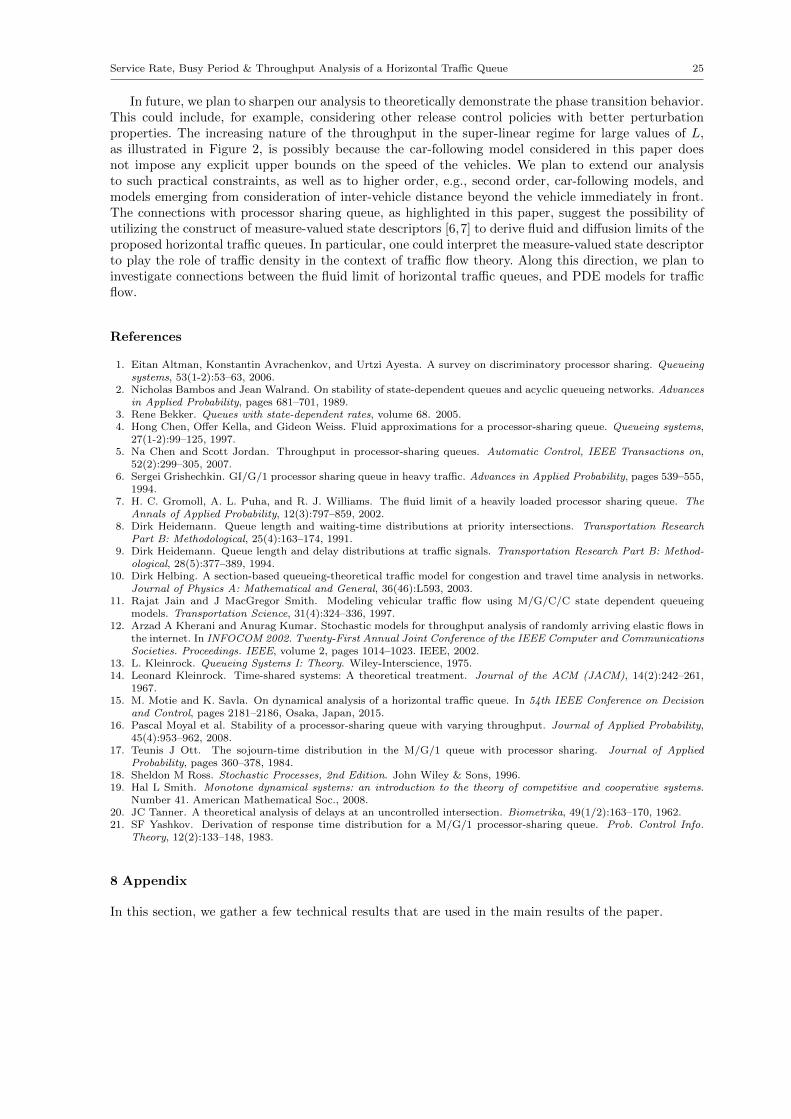
It is instructive to compare Figures 7(b) and 11(a), both of which depict throughput estimates forthe sub-linear case, however obtained from different methods, namely busy period distribution andbatch release control policy. Accordingly, one should bear in mind that the two bounds have differentqualifiers attached to them: the bound in Figure 7(b) is valid probabilistically only over a finite timehorizon, whereas the bound in Figure 11(a) is valid with probability one, although under a perturbationto the arrival process.
Finally, Figure 12 shows a good agreement between queue length bound suggested by Remark 3,and the corresponding numerical estimates in the linear case.
7 Conclusions
In this paper, we formulated and analyzed a novel horizontal traffic queue. A key characteristic of thisqueue is the state dependence of its service rate. We establish useful properties of the service ratedynamics. We also extend calculations for M/G/1 busy period distributions to our setting, even fornon-empty initial condition. These results allow us to provide tight results for throughput in the linearcase, and probabilistic bounds on queue length over finite time horizon in the super-linear case. We
24 Mohammad Motie, Ketan Savla
m0 0.2 0.4 0.6 0.8
log(6
max)
0
5
10
15
20
25
30
35
402 = 152 = 5
Fig. 10 Theoretical estimates of throughput from Theorems 4 for different values of η. The parameters used for this caseare: L = 1, ϕ = U[0,L], ψ = U[0,L], and w0 = 0 . Note that the vertical axis is in logarithmic scale.
m1.1 1.2 1.3 1.4 1.5 1.6 1.7 1.8
λmax
0
0.2
0.4
0.6
0.8
1
1.2
1.4
1.6
1.8Estimate from Theorem 5, η = 8Estimate from Theorem 5, η = 20Upper Range of Numerical Estimate
(a)
m1.1 1.2 1.3 1.4 1.5 1.6 1.7 1.8
λmax
0
5
10
15Estimate from Theorem 5, η = 3Estimate from Theorem 5, η = 10Upper Range of Numerical Estimate
(b)
Fig. 11 Theoretical estimates of throughput from Theorem 5, and numerical estimates from simulations for differentThe parameters used for this case are: ϕ = U[0,L], ψ = U[0,L], and (a) L = 1, (b) L = 100.
λ0.9 0.92 0.94 0.96 0.98
Que
ue L
engt
h
5
10
15
20
25
30
35
40
45
50Upper Bound by Remark 3Empirical Expectation
Fig. 12 Comparison between the empirical expectation of the queue length and the upper bound suggested by Remark 3.We let the simulations run up to time t = 80, 000. The parameters used for this case are: L = 1, m = 1, ϕ = δ0, ψ = δL.For these values, we have λmax = 1.
also study throughput under a batch release control policy, where the additional waiting induced bythe control policy is interpreted as a perturbation to the arrival process. We provide lower bound onthe throughput for a maximum permissible perturbation. In particular, if the allowable perturbationis sufficiently large, then this lower bound grows unbounded as m → 0+. Simulation results suggest asharp phase transition in the throughput as the car-following behavior transitions from super-linear tosub-linear regime.
Service Rate, Busy Period & Throughput Analysis of a Horizontal Traffic Queue 25
In future, we plan to sharpen our analysis to theoretically demonstrate the phase transition behavior.This could include, for example, considering other release control policies with better perturbationproperties. The increasing nature of the throughput in the super-linear regime for large values of L,as illustrated in Figure 2, is possibly because the car-following model considered in this paper doesnot impose any explicit upper bounds on the speed of the vehicles. We plan to extend our analysisto such practical constraints, as well as to higher order, e.g., second order, car-following models, andmodels emerging from consideration of inter-vehicle distance beyond the vehicle immediately in front.The connections with processor sharing queue, as highlighted in this paper, suggest the possibility ofutilizing the construct of measure-valued state descriptors [6,7] to derive fluid and diffusion limits of theproposed horizontal traffic queues. In particular, one could interpret the measure-valued state descriptorto play the role of traffic density in the context of traffic flow theory. Along this direction, we plan toinvestigate connections between the fluid limit of horizontal traffic queues, and PDE models for trafficflow.
References
1. Eitan Altman, Konstantin Avrachenkov, and Urtzi Ayesta. A survey on discriminatory processor sharing. Queueingsystems, 53(1-2):53–63, 2006.
2. Nicholas Bambos and Jean Walrand. On stability of state-dependent queues and acyclic queueing networks. Advancesin Applied Probability, pages 681–701, 1989.
3. Rene Bekker. Queues with state-dependent rates, volume 68. 2005.4. Hong Chen, Offer Kella, and Gideon Weiss. Fluid approximations for a processor-sharing queue. Queueing systems,
27(1-2):99–125, 1997.5. Na Chen and Scott Jordan. Throughput in processor-sharing queues. Automatic Control, IEEE Transactions on,
52(2):299–305, 2007.6. Sergei Grishechkin. GI/G/1 processor sharing queue in heavy traffic. Advances in Applied Probability, pages 539–555,
1994.7. H. C. Gromoll, A. L. Puha, and R. J. Williams. The fluid limit of a heavily loaded processor sharing queue. The
Annals of Applied Probability, 12(3):797–859, 2002.8. Dirk Heidemann. Queue length and waiting-time distributions at priority intersections. Transportation Research
Part B: Methodological, 25(4):163–174, 1991.9. Dirk Heidemann. Queue length and delay distributions at traffic signals. Transportation Research Part B: Method-
ological, 28(5):377–389, 1994.10. Dirk Helbing. A section-based queueing-theoretical traffic model for congestion and travel time analysis in networks.
Journal of Physics A: Mathematical and General, 36(46):L593, 2003.11. Rajat Jain and J MacGregor Smith. Modeling vehicular traffic flow using M/G/C/C state dependent queueing
models. Transportation Science, 31(4):324–336, 1997.12. Arzad A Kherani and Anurag Kumar. Stochastic models for throughput analysis of randomly arriving elastic flows in
the internet. In INFOCOM 2002. Twenty-First Annual Joint Conference of the IEEE Computer and CommunicationsSocieties. Proceedings. IEEE, volume 2, pages 1014–1023. IEEE, 2002.
13. L. Kleinrock. Queueing Systems I: Theory. Wiley-Interscience, 1975.14. Leonard Kleinrock. Time-shared systems: A theoretical treatment. Journal of the ACM (JACM), 14(2):242–261,
1967.15. M. Motie and K. Savla. On dynamical analysis of a horizontal traffic queue. In 54th IEEE Conference on Decision
and Control, pages 2181–2186, Osaka, Japan, 2015.16. Pascal Moyal et al. Stability of a processor-sharing queue with varying throughput. Journal of Applied Probability,
45(4):953–962, 2008.17. Teunis J Ott. The sojourn-time distribution in the M/G/1 queue with processor sharing. Journal of Applied
Probability, pages 360–378, 1984.18. Sheldon M Ross. Stochastic Processes, 2nd Edition. John Wiley & Sons, 1996.19. Hal L Smith. Monotone dynamical systems: an introduction to the theory of competitive and cooperative systems.
Number 41. American Mathematical Soc., 2008.20. JC Tanner. A theoretical analysis of delays at an uncontrolled intersection. Biometrika, 49(1/2):163–170, 1962.21. SF Yashkov. Derivation of response time distribution for a M/G/1 processor-sharing queue. Prob. Control Info.
Theory, 12(2):133–148, 1983.
8 Appendix
In this section, we gather a few technical results that are used in the main results of the paper.
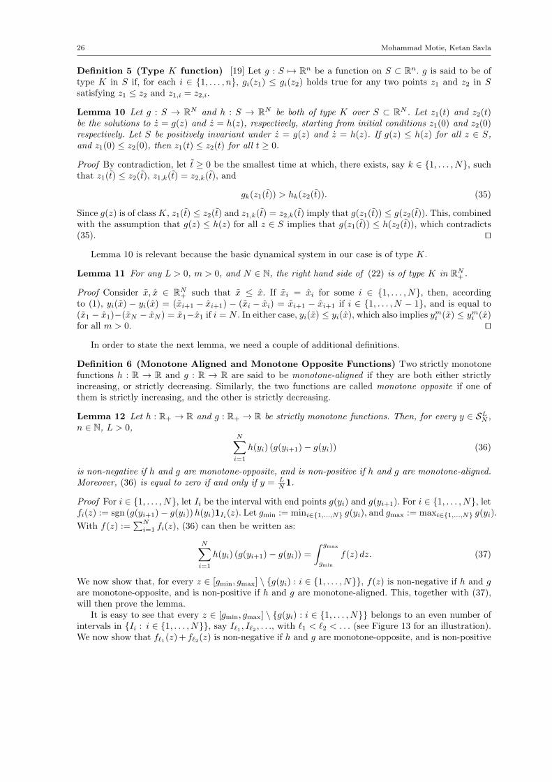
26 Mohammad Motie, Ketan Savla
Definition 5 (Type K function) [19] Let g : S 7→ Rn be a function on S ⊂ Rn. g is said to be oftype K in S if, for each i ∈ {1, . . . , n}, gi(z1) ≤ gi(z2) holds true for any two points z1 and z2 in Ssatisfying z1 ≤ z2 and z1,i = z2,i.
Lemma 10 Let g : S → RN and h : S → RN be both of type K over S ⊂ RN . Let z1(t) and z2(t)be the solutions to z = g(z) and z = h(z), respectively, starting from initial conditions z1(0) and z2(0)respectively. Let S be positively invariant under z = g(z) and z = h(z). If g(z) ≤ h(z) for all z ∈ S,and z1(0) ≤ z2(0), then z1(t) ≤ z2(t) for all t ≥ 0.
Proof By contradiction, let t ≥ 0 be the smallest time at which, there exists, say k ∈ {1, . . . , N}, suchthat z1(t) ≤ z2(t), z1,k(t) = z2,k(t), and
gk(z1(t)) > hk(z2(t)). (35)
Since g(z) is of class K, z1(t) ≤ z2(t) and z1,k(t) = z2,k(t) imply that g(z1(t)) ≤ g(z2(t)). This, combinedwith the assumption that g(z) ≤ h(z) for all z ∈ S implies that g(z1(t)) ≤ h(z2(t)), which contradicts(35). ut
Lemma 10 is relevant because the basic dynamical system in our case is of type K.
Lemma 11 For any L > 0, m > 0, and N ∈ N, the right hand side of (22) is of type K in RN+ .
Proof Consider x, x ∈ RN+ such that x ≤ x. If xi = xi for some i ∈ {1, . . . , N}, then, accordingto (1), yi(x) − yi(x) = (xi+1 − xi+1) − (xi − xi) = xi+1 − xi+1 if i ∈ {1, . . . , N − 1}, and is equal to(x1 − x1)−(xN − xN ) = x1−x1 if i = N . In either case, yi(x) ≤ yi(x), which also implies ymi (x) ≤ ymi (x)for all m > 0. ut
In order to state the next lemma, we need a couple of additional definitions.
Definition 6 (Monotone Aligned and Monotone Opposite Functions) Two strictly monotonefunctions h : R → R and g : R → R are said to be monotone-aligned if they are both either strictlyincreasing, or strictly decreasing. Similarly, the two functions are called monotone opposite if one ofthem is strictly increasing, and the other is strictly decreasing.
Lemma 12 Let h : R+ → R and g : R+ → R be strictly monotone functions. Then, for every y ∈ SLN ,n ∈ N, L > 0,
N∑i=1
h(yi) (g(yi+1)− g(yi)) (36)
is non-negative if h and g are monotone-opposite, and is non-positive if h and g are monotone-aligned.Moreover, (36) is equal to zero if and only if y = L
N 1.
Proof For i ∈ {1, . . . , N}, let Ii be the interval with end points g(yi) and g(yi+1). For i ∈ {1, . . . , N}, letfi(z) := sgn (g(yi+1)− g(yi))h(yi)1Ii(z). Let gmin := mini∈{1,...,N} g(yi), and gmax := maxi∈{1,...,N} g(yi).
With f(z) :=∑Ni=1 fi(z), (36) can then be written as:
N∑i=1
h(yi) (g(yi+1)− g(yi)) =
∫ gmax
gmin
f(z) dz. (37)
We now show that, for every z ∈ [gmin, gmax] \ {g(yi) : i ∈ {1, . . . , N}}, f(z) is non-negative if h and gare monotone-opposite, and is non-positive if h and g are monotone-aligned. This, together with (37),will then prove the lemma.
It is easy to see that every z ∈ [gmin, gmax] \ {g(yi) : i ∈ {1, . . . , N}} belongs to an even number ofintervals in {Ii : i ∈ {1, . . . , N}}, say I`1 , I`2 , . . ., with `1 < `2 < . . . (see Figure 13 for an illustration).We now show that f`1(z) + f`2(z) is non-negative if h and g are monotone-opposite, and is non-positive
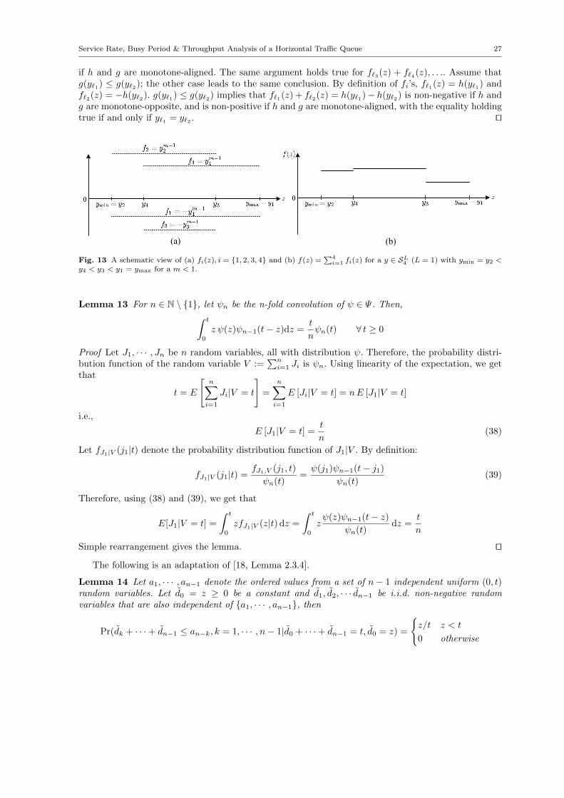
Service Rate, Busy Period & Throughput Analysis of a Horizontal Traffic Queue 27
if h and g are monotone-aligned. The same argument holds true for f`3(z) + f`4(z), . . .. Assume thatg(y`1) ≤ g(y`2); the other case leads to the same conclusion. By definition of fi’s, f`1(z) = h(y`1) andf`2(z) = −h(y`2). g(y`1) ≤ g(y`2) implies that f`1(z) + f`2(z) = h(y`1)− h(y`2) is non-negative if h andg are monotone-opposite, and is non-positive if h and g are monotone-aligned, with the equality holdingtrue if and only if y`1 = y`2 . ut
(a) (b)
Fig. 13 A schematic view of (a) fi(z), i = {1, 2, 3, 4} and (b) f(z) =∑4
i=1 fi(z) for a y ∈ SL4 (L = 1) with ymin = y2 <
y4 < y3 < y1 = ymax for a m < 1.
Lemma 13 For n ∈ N \ {1}, let ψn be the n-fold convolution of ψ ∈ Ψ . Then,∫ t
0
z ψ(z)ψn−1(t− z)dz =t
nψn(t) ∀ t ≥ 0
Proof Let J1, · · · , Jn be n random variables, all with distribution ψ. Therefore, the probability distri-bution function of the random variable V :=
∑ni=1 Ji is ψn. Using linearity of the expectation, we get
that
t = E
[n∑i=1
Ji|V = t
]=
n∑i=1
E [Ji|V = t] = nE [J1|V = t]
i.e.,
E [J1|V = t] =t
n(38)
Let fJ1|V (j1|t) denote the probability distribution function of J1|V . By definition:
fJ1|V (j1|t) =fJ1,V (j1, t)
ψn(t)=ψ(j1)ψn−1(t− j1)
ψn(t)(39)
Therefore, using (38) and (39), we get that
E[J1|V = t] =
∫ t
0
zfJ1|V (z|t) dz =
∫ t
0
zψ(z)ψn−1(t− z)
ψn(t)dz =
t
n
Simple rearrangement gives the lemma. ut
The following is an adaptation of [18, Lemma 2.3.4].
Lemma 14 Let a1, · · · , an−1 denote the ordered values from a set of n− 1 independent uniform (0, t)random variables. Let d0 = z ≥ 0 be a constant and d1, d2, · · · dn−1 be i.i.d. non-negative randomvariables that are also independent of {a1, · · · , an−1}, then
Pr(dk + · · ·+ dn−1 ≤ an−k, k = 1, · · · , n− 1|d0 + · · ·+ dn−1 = t, d0 = z) =
{z/t z < t
0 otherwise