Kernel-Based Manifold Learning for StatisticalAnalysis of Diffusion Tensor Images

Parmeshwar Khurd, Ragini Verma, and Christos Davatzikos

Section of Biomedical Image Analysis, Dept. of Radiology,University of Pennsylvania, Philadelphia, USA

khurdp@uphs.upenn.edu

Abstract. Diffusion tensor imaging (DTI) is an important modality tostudy white matter structure in brain images and voxel-based group-wisestatistical analysis of DTI is an integral component in most biomedicalapplications of DTI. Voxel-based DTI analysis should ideally satisfy twodesiderata: (1) it should obtain a good characterization of the statisticaldistribution of the tensors under consideration at a given voxel, whichtypically lie on a non-linear submanifold of �6, and (2) it should findan optimal way to identify statistical differences between two groups oftensor measurements, e.g., as in comparative studies between normaland diseased populations. In this paper, extending previous work on theapplication of manifold learning techniques to DTI, we shall present akernel-based approach to voxel-wise statistical analysis of DTI data thatsatisfies both these desiderata. Using both simulated and real data, weshall show that kernel principal component analysis (kPCA) can effec-tively learn the probability density of the tensors under consideration andthat kernel Fisher discriminant analysis (kFDA) can find good featuresthat can optimally discriminate between groups. We shall also presentresults from an application of kFDA to a DTI dataset obtained as partof a clinical study of schizophrenia.

1 Introduction

Diffusion tensor imaging (DTI) has become an important modality for studyingwhite matter structure in brain imaging and other biomedical applications [1].Several such applications require a group-wise statistical analysis of DT imageswhich can identify regional differences between two groups of DT images. How-ever, statistical analysis of DTI is complicated by the fact that we now have a3×3 positive-definite symmetric matrix or diffusion tensor at each voxel insteadof a single value as in the case of scalar images.

In conventional methods of performing such an analysis, scalar or vector im-ages are first computed from the DTI dataset and then spatially normalizedto a common template. A statistical p-value map is then computed from thesescalar or vector images with the application of standard tests for statistical in-ference. Commonly used scalar images for such analyses include the fractionalanisotropy (FA) and the apparent diffusion coefficient (ADC) [1]. Non-scalar fea-tures [2] such as the principal eigendirections of the tensors have also been used

N. Karssemeijer and B. Lelieveldt (Eds.): IPMI 2007, LNCS 4584, pp. 581–593, 2007.c© Springer-Verlag Berlin Heidelberg 2007

582 P. Khurd, R. Verma, and C. Davatzikos

in some analyses. However, a main disadvantage of these methods is that theydo not use the complete information available in the DTI dataset, but rathermake the a priori assumption that group differences will affect specific quantitiesto be extracted from the diffusion tensor, such as FA. Moreover, differences inthese scalar maps may be mutually difficult to interpret.

A voxel-based statistical analysis should ideally try to learn the density andthe manifold structure pertinent to the specific tensors under consideration anddetermine the degree of separation between two groups of tensors. Methods forstatistical analysis of tensors have been recently developed that utilize the fulltensor information by trying to learn the underlying structure of the data. Thesemethods fall into two categories: methods based upon Riemannian symmetricspaces [3,4] and methods based upon manifold learning [5]. Methods based uponRiemannian symmetric spaces [3,4] rely upon the assumption that the tensorsaround a given voxel from various subjects belong to a principal geodesic (sub)-manifold and that these tensors obey a normal distribution on that sub-manifold.The basic principle of these methods is sound, namely that statistical analysis oftensors must be restricted to the appropriate manifold of positive definite sym-metric tensors, which is known to be a cone embedded in �6. However, there isno guarantee that the representations of the tensors on this sub-manifold willhave normal distributions, and most importantly, restricting the analysis on themanifold of positive definite symmetric tensors is of little help in hypothesis test-ing studies, since the tensors measured at a given voxel or neighborhood froma particular set of brains typically lie on a much more restricted submanifold.Our main goal is to determine the statistical distribution of tensors on this sub-manifold. In the approaches based upon manifold learning [5], the focus wason learning embeddings (or features) parameterizing the underlying manifoldstructure of the tensors. The learned features belonged to a low-dimensional lin-ear manifold parameterizing the higher-dimensional tensor manifold and weresubsequently used for group-wise statistical analysis. The main problem withmanifold learning approaches [6] is that although they estimate the embeddingof the manifold that represents the tensor measurements fairly well, they fail toestimate the probability distribution (non-Gaussian) on the (flattened) manifolditself. From experiments with simulated data, we have found that such an ap-proach does not completely parameterize the probability density of the tensorsunder consideration and that the learned features do not always identify thedifferences between the two groups.

We shall present an integrated kernel-based approach to voxel-based analysisthat accurately estimates the underlying distribution of the tensor data, obtainsa highly informative linear representation for the tensors and uses this represen-tation to determine statistically optimal ways of separating the tensor data. Weshall build upon related approaches in [5]. We present our methods in Sec. 2 andthe results from various experiments on simulated and real data in Sec. 3.1 andSec. 3.2. We shall establish that higher-dimensional kernel principal componentanalysis (kPCA) features are very effective in learning the required probabilitydensity of the tensors from a voxel and that kernel Fisher discriminant analysis

Kernel-Based Manifold Learning for Statistical Analysis 583

(kFDA) can optimally discriminate between groups of tensors. We shall also ap-ply our methods to a clinical DTI dataset of healthy controls and schizophrenicpatients in Sec. 3.3. We conclude with Sec. 4.

2 Methods

2.1 Kernel-Based Approach to Group-Wise Voxel-Based DTIStatistical Analysis

A DT image consists of a 3 × 3 positive-definite symmetric matrix or tensor Tat each voxel in the image. We may represent this tensor as T =

∑3i=1 λivivT

i ,where λi > 0 and vi represent the eigenvalues and eigenvectors of the tensor,respectively. Pathology can bring about subtle changes in eigen values or angularchanges in the eigen vectors, that can be partially seen in measures of anisotropyand diffusivity computed from the tensor, such as FA and ADC, although eigenvector changes can only be seen in full tensor color maps. Group-wise voxel-based statistical analysis of DTI data involves normalizing all DT images toa common DTI template using a suitable technique [7,8,9] and then using anappropriate statistical test to infer regional differences between groups basedupon the tensors at (or around) a voxel. We form a voxel-based dataset bycollecting tensors from each location as samples. Such samples should ideallybe formed using the tensors at a voxel from all subjects, in conjunction withthe deformation field used to normalize the tensors. In this paper, we focus onthe former term, however our approach readily extends to the latter, as well asto neighborhood information from tensors around a voxel under consideration,albeit at the cost of increasing the dimensionality of the measurements and theembedding space. The samples in our voxel-based dataset will have unknownstatistical distributions on complex unknown non-linear manifolds. Therefore, itis particularly important to analyze the underlying structure in our dataset andto use this structure to estimate features that can identify group differences.

We have found that kernel-based techniques (kPCA and kFDA) are ideallysuited for performing such an analysis. The common idea behind kernel-basedtechniques is to transform the samples into a higher-dimensional reproduciblekernel Hilbert space (RKHS). Using the “kernel trick”, any algorithm that canbe written in terms of inner products in the RKHS, can be readily formulated inthe original space in terms of the kernel. Moreover, hyperplanes in the RKHS,such as the ones spanned by principal eigenvectors or the ones separating twosets of samples, become nonlinear hyper-surfaces in the original space, therebyallowing us to nonlinearly span or separate groups of samples for the purposesof density estimation or classification, respectively. We can hence easily performvarious calculations such as computing projections onto directions in the RKHS,although we cannot visualize this space itself. Figure 1 illustrates the idea behindobtaining such projections.

From our voxel-based samples, we can obtain highly informative projectionsusing the kPCA technique, as described later in Sec. 2.2. Although we couldextract useful features from this higher-dimensional kPCA representation to aid

584 P. Khurd, R. Verma, and C. Davatzikos

Φ

Original Space RKHS

The mapping Φ takes points (marked

with crosses) from the original space

to the RKHS. Hyperplanes having con-

stant projections onto a vector in the

RKHS become curved lines in the orig-

inal space. Such curved lines can give

us important insight into how the corre-

sponding RKHS projection parameter-

izes the original points.

Fig. 1. Kernel-based projections

us in inferring differences between groups, it would be better to perform thisinference step in an automated and optimal manner. For this purpose, we shalluse the kFDA technique described in Sec. 2.3, which finds scalar projections ontoa single RKHS direction that can optimally discriminate between groups. Havingobtained our kernel-based features, we can then apply standard statistical testssuch as the Hotelling T 2 test in the case of kPCA or the t-test in the case of thekFDA to obtain a voxel-wise p-value map. We note that the projections foundby kPCA and kFDA lie along directions in the linear RKHS and hence lineartests for statistical inference can be reliably applied to these projections in orderto identify separation between groups. Regions with low p-values indicate theregions with significant differences between the two groups.

Before we present the kPCA and kFDA techniques in detail, here is a briefnote on our mathematical conventions: We denote vectors by bold-faced lowercase letters, e.g. x, and matrices by upper-case letters, e.g. A. We use e to denotethe vector of all 1’s and I to denote the identity matrix. We occasionally use em

to denote a vector of all 1’s in m-dimensional space. We use the superscripts T

and −1 to denote the matrix transpose and the matrix inverse respectively. Wedenote the sample mean of a set of vectors {xi, i = 1, · · · , K} by x̄. We denotethe inner product of two vectors xi,xj by < xi,xj >. We shall assume that ourgroup-wise study involves a statistical analysis of the DT images of N subjects,with N+ subjects in one class (the positive class) and the remaining N− subjectsin a second class (the negative class).

2.2 Kernel Principal Component Analysis (kPCA)

We now describe the kPCA technique [10] which can find a rich linear repre-sentation of our voxel-based samples as well as provide an accurate estimate ofthe probability density underlying these samples. In conventional PCA, we findout principal directions in the vector space of the samples that maximize thevariance of the projections of the samples along those directions and which alsominimize the least-squares representation error for the samples. In kPCA, wefind similar principal eigendirections in the higher-dimensional RKHS. Let usdenote the nonlinear mapping of point x into the Hilbert space by Φ(x), and letus denote the underlying kernel by k(., .), where < Φ(xi),Φ(xj) >= k(xi,xj).

Kernel-Based Manifold Learning for Statistical Analysis 585

Since a principal eigenvector v in the higher-dimensional Hilbert space lies in thespan of the vectors Φ(xi) − Φ̄, i = 1, · · · , N , it can be conveniently representedas v =

∑i αi(Φ(xi) − Φ̄), where α is an N -dimensional vector. Projections of

any sample along the eigenvector v can now be conveniently computed usingthis new representation in the kernel basis.

The entire kPCA procedure is summarized below [6]:

1. Form the kernel matrix K, where Kij = k(xi,xj), i = 1, · · · , N, j = 1, · · · , N.2. Center the kernel matrix to obtain Kc = (I − 1

N eeT )K(I − 1N eeT ).

3. Eigen-decompose Kc to obtain its eigenvectors α(i) and eigenvalues λi, i =1, · · · , N .

4. Normalize the eigenvectors α(i) to have length 1√λi

so that the eigenvectors

v(i) in the RKHS have unit length.5. The ith kPCA component for training sample xk is given by:

< Φ(xk) − Φ̄,v(i) >= λiα(i)k

6. For a general test point x, the ith kPCA component is:< Φ(x) − Φ̄,v(i) >=

∑m α

(i)m k(x,xm) − 1

N

∑m,n α

(i)m k(x,xn)

In addition to finding the orthogonal directions of maximal variance in thehigher-dimensional RKHS, kPCA also provides an estimate of the probabilitydensity underlying the samples. It has been pointed out in [11] that kPCA witha Gaussian radial basis function kernel amounts to orthogonal series density es-timation using Hermite polynomials. In Sec. 3.1, we shall present a simulatedexample (see Fig. 2) where kPCA obtained a very good parameterization of thedensity underlying the dataset. We also note that the kPCA components consti-tute a linear representation of the dataset in the RKHS, which considerably sim-plifies any further analysis such as the application of tests for statistical inference.

2.3 Kernel Fisher Discriminant Analysis (kFDA)

As described earlier, often the goal is not only to nonlinearly approximate theprobability density from a number of samples, as in Sec. 2.2, but also to non-linearly separate two groups of samples belonging to separate classes. We nowexamine this problem using kernel-based discriminants. We describe the kFDAtechnique [10,12], which focuses on finding nonlinear projections of the tensor-ial data which can optimally discriminate between the two groups. Kernel FDAfinds a direction w in the higher-dimensional RKHS so that a projection alongthis direction maximizes a separability measure known as the Rayleigh coeffi-cient (or the Fisher discriminant ratio). Let Φ̄+ denote the Hilbert-space meanfor the samples in the positive class, corresponding to the N+ DT images fromthe first group, and let Φ̄− denote the mean for the negative class, correspondingto the N− DT images from the second group. Let Σ+ and Σ− denote the sam-ple covariance matrices for the positive and negative classes respectively. TheRayleigh coefficient is then given by:

J(w) =(wT (Φ̄+ − Φ̄−))2

wT (Σ+ + Σ− + cI)w,

586 P. Khurd, R. Verma, and C. Davatzikos

where the scalar c is used to introduce regularization. As in kPCA, the optimalsolution w∗ maximizing J(w) can again be conveniently represented using thesamples, i.e. w∗ =

∑n α∗

nΦ(xn), and projections along this direction can beeasily obtained. A convenient analytical solution for α∗ is provided in [12]:

α∗ =1c

[I − J(cI + JKJ)−1JK

]a,

where a = a+ − a−, a+ =[ 1

N+eN+

0

]

, a− =[

01

N−eN−

]

, J =[

J+ 00 J−

]

,

J+ =1

√N+

(I − 1

N+eN+eT

N+

), J− =

1√

N−

(I − 1

N−eN−eT

N−

),

and where K represents the un-centered kernel matrix. An alternative quadraticprogramming approach to obtaining the solution α∗ is provided in [10].

To summarize, we have presented the kPCA technique which can estimatethe probability density and yield a rich linear representation for any voxel-basedtensor dataset and the kFDA technique which uses this representation to extractfeatures that can identify group differences in a statistically optimal manner.

3 Results and Discussion

We have applied the kernelized framework to the group analysis of real and sim-ulated DTI data with the aim of demonstrating that kPCA is able to capture thestatistical distribution underlying such datasets and that application of kFDAfacilitates optimal group-based separation.

3.1 Statistical Analysis of Simulated Tensors

We shall first apply our kernelized framework to group analysis of simulated(non-imaging) tensor datasets where we know the ground-truth underlying struc-ture in the dataset and can therefore easily validate our results. We considertensor datasets with changes in the principal eigenvalue as well as in one ofthe angles describing the principal eigendirection. Such subtle changes emu-late pathology-induced changes that affect the eigenvalue and eigenvector andan analysis of subtle changes of this nature may be of particular importance instudying complex brain disorders such as schizophrenia which result in non-focalregional changes. We have found that kPCA is well-suited for parameterizing thedensity for such datasets and that kFDA can effectively highlight the differencesthat discriminate between groups. For ease of visualization, we present repre-sentative results on a dataset with variation in the radial and angular directionsinstead of on a tensorial dataset with changes in the principal eigenvalue andeigendirection.

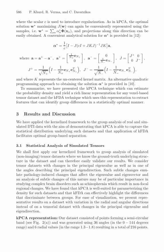
kPCA representation: Our dataset consisted of points forming a semi-circularband (see Fig. 2(a)) and was generated using 36 angles (in the 0 − 144 degreesrange) and 6 radial values (in the range 1.3−1.8) resulting in a total of 216 points.

Kernel-Based Manifold Learning for Statistical Analysis 587

−1 0 1

0

0.5

1

1.5

2Density Estimate

−1 0 1

0

0.5

1

1.5

2

0.05

0.1

0.15

Component 1

−1 0 1

0

0.5

1

1.5

2

−0.5

0

0.5

(a) (b) (c)Component 2

−1 0 1

0

0.5

1

1.5

2

−0.6

−0.4

−0.2

0

0.2

Component 3

−1 0 1

0

0.5

1

1.5

2

−0.4

−0.2

0

0.2

0.4

Component 4

−1 0 1

0

0.5

1

1.5

2

−0.4

−0.2

0

0.2

(d) (e) (f)Component 5

−1 0 1

0

0.5

1

1.5

2

−0.3

−0.2

−0.1

0

0.1

0.2

0.3

Component 6

−1 0 1

0

0.5

1

1.5

2

−0.3

−0.2

−0.1

0

0.1

0.2

Component 7

−1 0 1

0

0.5

1

1.5

2

−0.3

−0.2

−0.1

0

0.1

0.2

0.3

0.4

(g) (h) (i)

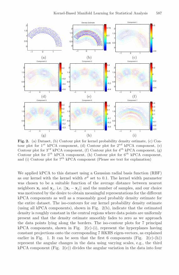
Fig. 2. (a) Dataset, (b) Contour plot for kernel probability density estimate, (c) Con-tour plot for 1st kPCA component, (d) Contour plot for 2nd kPCA component, (e)Contour plot for 3rd kPCA component, (f) Contour plot for 4th kPCA component, (g)Contour plot for 5th kPCA component, (h) Contour plot for 6th kPCA component,and (i) Contour plot for 7th kPCA component (Please see text for explanation)

We applied kPCA to this dataset using a Gaussian radial basis function (RBF)as our kernel with the kernel width σ2 set to 0.1. The kernel width parameterwas chosen to be a suitable function of the average distance between nearestneighbors xi and xj , i.e. ||xi − xj || and the number of samples, and our choicewas motivated by the desire to obtain meaningful representations for the differentkPCA components as well as a reasonably good probably density estimate forthe entire dataset. The iso-contours for our kernel probability density estimate(using all kPCA components), shown in Fig. 2(b), indicate that the estimateddensity is roughly constant in the central regions where data points are uniformlypresent and that the density estimate smoothly fades to zero as we approachthe data points lying along the borders. The iso-contour plots for 7 principalkPCA components, shown in Fig. 2(c)-(i), represent the hyperplanes havingconstant projections onto the corresponding 7 RKHS eigen-vectors, as explainedearlier in Fig. 1. It can be seen that the first 6 components (Fig. 2(c)-(h))represent the angular changes in the data using varying scales, e.g., the thirdkPCA component (Fig. 2(e)) divides the angular variation in the data into four

588 P. Khurd, R. Verma, and C. Davatzikos

−1 −0.5 0 0.5 1 1.5

0

0.5

1

1.5

2

−1 −0.5 0 0.5 1 1.5

0

0.5

1

1.5

2

−1 −0.5 0 0.5 1 1.5

0

0.5

1

1.5

2

(a) (c) (e)

−1 0 1

0.5

1

1.5

−1

−0.5

0

0.5

1

−1 0 1

0.5

1

1.5

−0.1

−0.05

0

0.05

0.1

0.15

0.2

−1 0 1

0.5

1

1.5

−0.4

−0.2

0

0.2

0.4

(b) (d) (f)

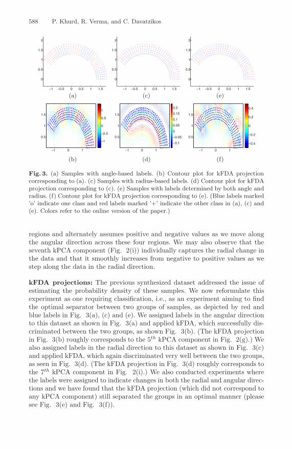
Fig. 3. (a) Samples with angle-based labels. (b) Contour plot for kFDA projectioncorresponding to (a). (c) Samples with radius-based labels. (d) Contour plot for kFDAprojection corresponding to (c). (e) Samples with labels determined by both angle andradius. (f) Contour plot for kFDA projection corresponding to (e). (Blue labels marked’o’ indicate one class and red labels marked ’+’ indicate the other class in (a), (c) and(e). Colors refer to the online version of the paper.)

regions and alternately assumes positive and negative values as we move alongthe angular direction across these four regions. We may also observe that theseventh kPCA component (Fig. 2(i)) individually captures the radial change inthe data and that it smoothly increases from negative to positive values as westep along the data in the radial direction.

kFDA projections: The previous synthesized dataset addressed the issue ofestimating the probability density of these samples. We now reformulate thisexperiment as one requiring classification, i.e., as an experiment aiming to findthe optimal separator between two groups of samples, as depicted by red andblue labels in Fig. 3(a), (c) and (e). We assigned labels in the angular directionto this dataset as shown in Fig. 3(a) and applied kFDA, which successfully dis-criminated between the two groups, as shown Fig. 3(b). (The kFDA projectionin Fig. 3(b) roughly corresponds to the 5th kPCA component in Fig. 2(g).) Wealso assigned labels in the radial direction to this dataset as shown in Fig. 3(c)and applied kFDA, which again discriminated very well between the two groups,as seen in Fig. 3(d). (The kFDA projection in Fig. 3(d) roughly corresponds tothe 7th kPCA component in Fig. 2(i).) We also conducted experiments wherethe labels were assigned to indicate changes in both the radial and angular direc-tions and we have found that the kFDA projection (which did not correspond toany kPCA component) still separated the groups in an optimal manner (pleasesee Fig. 3(e) and Fig. 3(f)).

Kernel-Based Manifold Learning for Statistical Analysis 589

(a) (b)

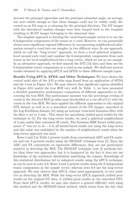
Fig. 4. (a) ROI with changes (high-lighted) overlaid on the template FAmap. (b) kFDA voxel-wise p-map (withsignificant low p-values highlighted)overlaid on the same FA map. Low p-value regions in (b) match the true ROIin (a).

(a) (b)

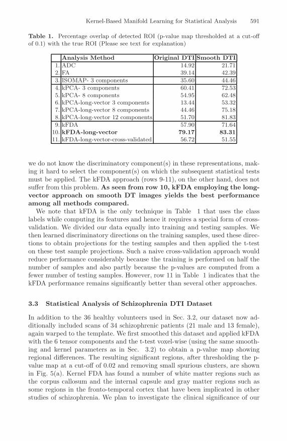
Fig. 5. (a) Schizophrenia kFDA p-mapthresholded at 0.02 and overlaid onthe template FA map. (b) Schizophre-nia kFDA p-map thresholded using afalse discovery rate of 0.18 and overlaidon the template FA map. Significantp-values after thresholding are high-lighted in (a), (b).

Comparison to manifold learning: Manifold learning techniques such asISOMAP (isometric mapping) [5] have also been proposed for DTI statisticalanalysis. We performed such an analysis using two approaches, ISOMAP [6], onthe lines of [5], and MVU (maximum variance unfolding) [13], both of whichcorrectly identify the underlying manifold of dimension 2 when applied to thedataset in Fig. 2(a), with MVU doing better than ISOMAP in separating theangular and radial changes in the data into its two components. An applicationof the Hotelling T 2 test on the MVU or ISOMAP embeddings, when grouplabels were assigned as in Figs. 3(a) or 3(c), yielded higher p-values, indicatingless significant differences, than those found by applying a t-test on the kFDAprojections or on the appropriate kPCA components, indicating that both MVUand ISOMAP were unable to identify the statistical distribution on the manifoldlike kPCA or determine projections like kFDA that separate the groups.

Having successfully validated our methods on a simulated non-imaging datasetwith radial and angular variation, we shall now validate them on real DTI datawith simulated changes in both the tensor eigenvalues and eigenvectors thatemulate this joint radial and angular variation.

3.2 Statistical Analysis of DTI Datasets with Simulated Changes

Dataset Description: Our DTI dataset consisted of scans of 36 healthy vol-unteers (17 male and 19 female), acquired at dimensions 128 × 128 × 40 and avoxel size of 1.72×1.72×3.0 mm. These DT images were warped to a template,which was chosen as the scan of an additional healthy subject. We then iden-tified an ROI on the template in the corpus callosum, as shown in Fig. 4(a),and introduced random changes in the principal eigenvalue and the azimuthalangle for the principal eigenvector of each tensor into the appropriate ROI forall unwarped subject DT images. The random changes were designed to slightly

590 P. Khurd, R. Verma, and C. Davatzikos

increase the principal eigenvalue and the principal azimuthal angle, on average,but were subtle enough so that these changes could not be visibly easily dis-cerned on an FA map or a colormap for the principal direction. The DT imageswith the introduced random changes were then warped back to the templateresulting in 36 DT images belonging to the abnormal class.

The simplest approach to forming the voxel-based sample vector is to use the6-independent components of the tensor at a voxel. However, we can potentiallyobtain more significant regional differences by incorporating neighborhood infor-mation around a voxel into our samples, in two different ways. In one approach,which we call the “long-vector” approach, we form a local spherical neighbor-hood around each voxel and combine the 6-independent components from eachtensor in the local neighborhood into a long vector, which we use as our sample.In an alternative approach, we first smooth the DTI [14] data and then use the6-independent tensor components at a voxel as our sample. We shall now presentresults obtained by applying kPCA and kFDA to these different sample types.

Results Using kPCA, kFDA and Other Techniques: We have shown thecentral axial slice of the 3-D p-value map found from an application of kFDAand the t-test in Figure 4(b). We may observe that significant regions identifiedin Figure 4(b) match the true ROI very well. In Table 1, we have presenteda detailed quantitative performance comparison of different approaches to dis-covering the true ROI. Our performance measure was the percentage overlap ofvoxels in the detected ROI (p-value map thresholded at a cut-off of 0.1) with thevoxels in the true ROI. We have applied the different approaches to the originalDTI dataset as well as to a smoothed version of the DT images, smoothed inthe Log-Euclidean domain [14] using an isotropic truncated Gaussian filter withthe filter σ set to 4 mm . This choice for smoothing yielded good results for thetechnique in [5]. For the long-vector results, we used a spherical neighborhoodof 4 mm radius that contained 39 voxels. The Gaussian RBF kernel width para-meter σ2 was set to 4e − 4 in all kernel-based results not using the long-vectorand this value was multiplied by the number of neighborhood voxels when thelong-vector approach was used.

Rows 1 and 2 in Table 1 present results from conventional ADC and FA analy-ses and row 3 presents results using the ISOMAP technique from [5]. Since theADC and FA concentrate on eigenvalue differences, they are not particularlysensitive in detecting the ROI. The ISOMAP technique (row 3) performs bet-ter than these two approaches, but it is hampered by the fact it does not useknowledge of the statistical distribution underlying the tensors. Knowledge ofthis statistical distribution led to enhanced results using the kPCA technique,as can be seen in rows 4-8. Rows 4 and 5 present results using the 6 independenttensor components as the sample vector, whereas rows 6-8 use the long-vectorapproach. We may observe that kPCA, when used appropriately, is very sensi-tive in detecting the ROI. While the long-vector kPCA approach yielded poorresults on the original DT data, it yielded good results on the smoothed DTI.From these kPCA results, we may also observe a general difficulty with usingthis method and the ISOMAP-based method, which stems from the fact that

Kernel-Based Manifold Learning for Statistical Analysis 591

Table 1. Percentage overlap of detected ROI (p-value map thresholded at a cut-offof 0.1) with the true ROI (Please see text for explanation)

Analysis Method Original DTI Smooth DTI1. ADC 14.92 21.712. FA 39.14 42.393. ISOMAP- 3 components 35.60 44.464. kPCA- 3 components 60.41 72.535. kPCA- 8 components 54.95 62.486. kPCA-long-vector 3 components 13.44 53.327. kPCA-long-vector 8 components 44.46 75.188. kPCA-long-vector 12 components 51.70 81.839. kFDA 57.90 71.64

10. kFDA-long-vector 79.17 83.3111. kFDA-long-vector-cross-validated 56.72 51.55

we do not know the discriminatory component(s) in these representations, mak-ing it hard to select the component(s) on which the subsequent statistical testsmust be applied. The kFDA approach (rows 9-11), on the other hand, does notsuffer from this problem. As seen from row 10, kFDA employing the long-vector approach on smooth DT images yields the best performanceamong all methods compared.

We note that kFDA is the only technique in Table 1 that uses the classlabels while computing its features and hence it requires a special form of cross-validation. We divided our data equally into training and testing samples. Wethen learned discriminatory directions on the training samples, used these direc-tions to obtain projections for the testing samples and then applied the t-teston these test sample projections. Such a naive cross-validation approach wouldreduce performance considerably because the training is performed on half thenumber of samples and also partly because the p-values are computed from afewer number of testing samples. However, row 11 in Table 1 indicates that thekFDA performance remains significantly better than several other approaches.

3.3 Statistical Analysis of Schizophrenia DTI Dataset

In addition to the 36 healthy volunteers used in Sec. 3.2, our dataset now ad-ditionally included scans of 34 schizophrenic patients (21 male and 13 female),again warped to the template. We first smoothed this dataset and applied kFDAwith the 6 tensor components and the t-test voxel-wise (using the same smooth-ing and kernel parameters as in Sec. 3.2) to obtain a p-value map showingregional differences. The resulting significant regions, after thresholding the p-value map at a cut-off of 0.02 and removing small spurious clusters, are shownin Fig. 5(a). Kernel FDA has found a number of white matter regions such asthe corpus callosum and the internal capsule and gray matter regions such assome regions in the fronto-temporal cortex that have been implicated in otherstudies of schizophrenia. We plan to investigate the clinical significance of our

592 P. Khurd, R. Verma, and C. Davatzikos

findings in future work. (We note that we found similar significant regions whenthe p-value maps were alternatively thresholded using a false discovery rate [15]of 0.18, as shown in Fig. 5(b).)

4 Conclusion

Using both simulated and real data, we have established that kernel-based meth-ods pave the way to resolving major issues in group-wise DTI statistical analysis,namely, the density estimation of voxel-based tensors (in the presence of non-linearity), the appropriate representation of these tensors on a manifold and thesubsequent use of this representation in the identification of features that canoptimally identify region-based group differences. In particular, we have shownthat kFDA can form the basis of a highly sensitive method for group-wise DTIstatistical analysis. Such a method can open up numerous avenues of research invarious DTI applications requiring large scale group analysis such as studies ofvarious brain disorders involving prognosis, diagnosis or progression of disease.Future work will involve optimal kernel selection in kFDA [12] and more sophis-ticated cross-validation of our kFDA results using permutation tests on the DTIdataset with simulated changes as well as on the schizophrenia DTI dataset.

Acknowledgements

This work was supported by the National Institute of Health via grantsR01MH070365, R01MH079938 and R01MH060722.

References

1. LeBihan, D., Mangin, J.F., et al.: Diffusion tensor imaging: Concepts and applica-tions. J. of Magnetic Resonance Imaging 13, 534–546 (2001)

2. Wu, Y.C., Field, A.S., et al.: Quantitative analysis of diffusion tensor orientation:Theoretical framework. Magnetic Resonance in Medicine 52, 1146–1155 (2004)

3. Lenglet, C., Rousson, M., Deriche, R., Faugeras, O.: Statistics on the manifold ofmultivariate normal distributions: Theory and application to diffusion tensor MRIprocessing. Journal of Math. Imaging and Vision 25(3), 423–444 (2006)

4. Fletcher, P.T., Joshi, S.: Principal geodesic analysis on symmetric spaces: Statisticsof diffusion tensors. In: Sonka, M., Kakadiaris, I.A., Kybic, J. (eds.) ComputerVision and Mathematical Methods in Medical and Biomedical Image Analysis.LNCS, vol. 3117, pp. 87–98. Springer, Heidelberg (2004)

5. Verma, R., Davatzikos, C.: Manifold based analysis of diffusion tensor images usingisomaps. In: IEEE Int. Symp. on Biomed, Imaging, pp. 790–793. IEEE, Washing-ton, DC, USA (2006)

6. Burges, C.: Geometric Methods for Feature Extraction and Dimensional Reduction.In: Data Mining and Knowledge Discovery Handbook, Kluwer Academic Publish-ers, Dordrecht (2005)

Kernel-Based Manifold Learning for Statistical Analysis 593

7. Zhang, H., Yushkevich, P., et al.: Deformable registration of diffusion tensor MRimages with explicit orientation optimization. Medical Image Analysis 10(5), 764–785 (2006)

8. Cao, Y., Miller, M., Mori, S., Winslow, R., Younes, L.: Diffeomorphic matching ofdiffusion tensor images. In: CVPR-MMBIA, 67 (2006)

9. Xu, D., Mori, S., Shen, D., van Zijl, P., Davatzikos, C.: Spatial normalization ofdiffusion tensor fields. Magnetic Resonance in Medicine 50(1), 175–182 (2003)

10. Scholkopf, B., Smola, A.: Learning with Kernels. The MIT Press, Cambridge, MA(2002)

11. Girolami, M.: Orthogonal series density estimation and the kernel eigenvalue prob-lem. Neural Computation 14(3), 669–688 (2002)

12. Kim, S.J., Magnani, A., Boyd, S.: Optimal kernel selection in kernel Fisher dis-criminant analysis. In: ACM Int. Conf. on Machine Learning 2006 (2006)

13. Saul, L.K., Weinberger, K.Q., Ham, J.H., Sha, F., Lee, D.D.: Spectral methods fordimensionality reduction. In: Semisupervised Learning, MIT Press, Cambridge,MA (2006)

14. Arsigny, V., Fillard, P., et al.: Medical Image Computing and Computer-AssistedIntervention. In: Duncan, J.S., Gerig, G. (eds.) MICCAI 2005. LNCS, vol. 3749,pp. 115–122. Springer, Heidelberg (2005)

15. Genovese, C., Lazar, N., Nichols, T.: Thresholding of statistical maps in functionalneuroimaging using the false discovery rate. NeuroImage 15, 870–878 (2002)