
katznelson-linalgebra
185
7/27/2019 katznelson-linalgebra http://slidepdf.com/reader/full/katznelson-linalgebra 1/185 A (TERSE) INTRODUCTION TO Linear Algebra Yitzhak Katznelson And Yonatan R. Katznelson (DRAFT)
-
Upload
saradharamachandran -
Category
Documents
-
view
213 -
download
0
Transcript of katznelson-linalgebra

7/27/2019 katznelson-linalgebra
http://slidepdf.com/reader/full/katznelson-linalgebra 1/185
A (TERSE) INTRODUCTION TO
Linear Algebra
Yitzhak Katznelson
And
Yonatan R. Katznelson
(DRAFT)

7/27/2019 katznelson-linalgebra
http://slidepdf.com/reader/full/katznelson-linalgebra 2/185

7/27/2019 katznelson-linalgebra
http://slidepdf.com/reader/full/katznelson-linalgebra 3/185
Contents
I Vector spaces 1
1.1 Vector spaces . . . . . . . . . . . . . . . . . . . . . . . . . 1
1.2 Linear dependence, bases, and dimension . . . . . . . . . . 9
1.3 Systems of linear equations. . . . . . . . . . . . . . . . . . 15
II Linear operators and matrices 27
2.1 Linear Operators (maps, transformations) . . . . . . . . . . 27
2.2 Operator Multiplication . . . . . . . . . . . . . . . . . . . . 31
2.3 Matrix multiplication. . . . . . . . . . . . . . . . . . . . . 32
2.4 Matrices and operators. . . . . . . . . . . . . . . . . . . . 36
2.5 Kernel, range, nullity, and rank . . . . . . . . . . . . . . . . 40
2.6 Normed finite dimensional linear spaces . . . . . . . . . . . 44
III Duality of vector spaces 49
3.1 Linear functionals . . . . . . . . . . . . . . . . . . . . . . 49
3.2 The adjoint . . . . . . . . . . . . . . . . . . . . . . . . . . 53
IV Determinants 57
4.1 Permutations . . . . . . . . . . . . . . . . . . . . . . . . . 57
4.2 Multilinear maps . . . . . . . . . . . . . . . . . . . . . . . 60
4.3 Alternating n-forms . . . . . . . . . . . . . . . . . . . . . . 63
4.4 Determinant of an operator . . . . . . . . . . . . . . . . . . 65
4.5 Determinant of a matrix . . . . . . . . . . . . . . . . . . . 67
iii
7/27/2019 katznelson-linalgebra
http://slidepdf.com/reader/full/katznelson-linalgebra 4/185
IV Contents
V Invariant subspaces 73
5.1 Invariant subspaces . . . . . . . . . . . . . . . . . . . . . . 73
5.2 The minimal polynomial . . . . . . . . . . . . . . . . . . . 77
5.3 Reducing. . . . . . . . . . . . . . . . . . . . . . . . . . . . 84
5.4 Semisimple systems. . . . . . . . . . . . . . . . . . . . . . 90
5.5 Nilpotent operators . . . . . . . . . . . . . . . . . . . . . . 93
5.6 The cyclic decomposition . . . . . . . . . . . . . . . . . . . 96
5.7 The Jordan canonical form . . . . . . . . . . . . . . . . . . 100
5.8 Functions of an operator . . . . . . . . . . . . . . . . . . . 103
VI Operators on inner-product spaces 107
6.1 Inner-product spaces . . . . . . . . . . . . . . . . . . . . . 107
6.2 Duality and the Adjoint. . . . . . . . . . . . . . . . . . . 115
6.3 Self-adjoint operators . . . . . . . . . . . . . . . . . . . . . 117
6.4 Normal operators. . . . . . . . . . . . . . . . . . . . . . . 122
6.5 Unitary and orthogonal operators . . . . . . . . . . . . . . . 124
6.6 Positive definite operators. . . . . . . . . . . . . . . . . . . 125
6.7 Polar decomposition . . . . . . . . . . . . . . . . . . . . . 126
6.8 Contractions and unitary dilations . . . . . . . . . . . . . . 130
VII Additional topics 133
7.1 Quadratic forms . . . . . . . . . . . . . . . . . . . . . . . . 133
7.2 Positive matrices . . . . . . . . . . . . . . . . . . . . . . . 1377.3 Nonnegative matrices . . . . . . . . . . . . . . . . . . . . . 140
7.4 Stochastic matrices. . . . . . . . . . . . . . . . . . . . . . 147
7.5 Matrices with integer entries, Unimodular matrices . . . . . 149
7.6 Representation of finite groups . . . . . . . . . . . . . . . . 149
A Appendix 157
A.1 Equivalence relations — partitions. . . . . . . . . . . . . . . 157
A.2 Maps . . . . . . . . . . . . . . . . . . . . . . . . . . . . . 158
A.3 Groups . . . . . . . . . . . . . . . . . . . . . . . . . . . . . 159
A.4 Group actions . . . . . . . . . . . . . . . . . . . . . . . . . 162

7/27/2019 katznelson-linalgebra
http://slidepdf.com/reader/full/katznelson-linalgebra 5/185
Contents V
A.5 Fields, Rings, and Algebras . . . . . . . . . . . . . . . . . 164
A.6 Polynomials . . . . . . . . . . . . . . . . . . . . . . . . . . 168
Index 175

7/27/2019 katznelson-linalgebra
http://slidepdf.com/reader/full/katznelson-linalgebra 6/185
VI Contents

7/27/2019 katznelson-linalgebra
http://slidepdf.com/reader/full/katznelson-linalgebra 7/185
Chapter I
Vector spaces
1.1 Vector spaces
The notions of group and field are defined in the Appendix: A.3 and
A.5.1 respectively.
The fieldsQ (of rational numbers), R (of real numbers), and C (of com-
plex numbers) are familiar, and are the most commonly used. Less famil-
iar, yet very useful, are the finite fields Z p; in particular Z2 = {0, 1} with
1 + 1 = 0, see A.5.1. Most of the notions and results we discuss are valid
for vector spaces over arbitrary underlying fields. When we do not need to
specify the underlying field we denote it by the generic F and refer to its ele-
ments as scalars. Results that require specific fields will be stated explicitly
in terms of the appropriate field.
1.1.1 DEFINITION: A vector space V
over a field F is an abeliangroup (the group operation written as addition) and a binary product (a, v) →av of F×V into V , satisfying the following conditions:
v-s 1. 1 v = v
v-s 2. a(bv) = (ab)v,
v-s 3. (a + b)v = av + bv, a(v + u) = av + au.
Other properties are derived from these—for example:
0v = (1
−1)v = v
−v = 0.
1
7/27/2019 katznelson-linalgebra
http://slidepdf.com/reader/full/katznelson-linalgebra 8/185
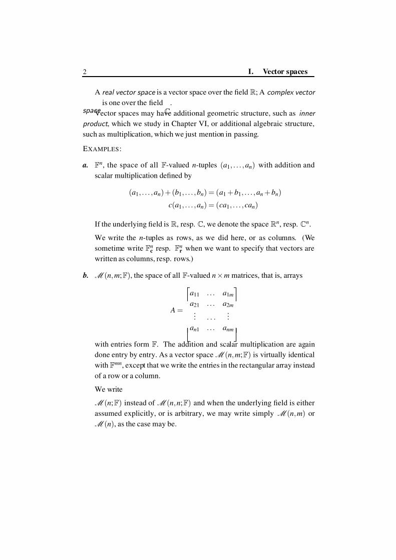
2 I. Vector spaces
A real vector space is a vector space over the field R; A complex vector
space is one over the field
C.
Vector spaces may have additional geometric structure, such as inner
product , which we study in Chapter VI, or additional algebraic structure,
such as multiplication, which we just mention in passing.
EXAMPLES:
a. Fn, the space of all F-valued n-tuples (a1, . . . , an) with addition and
scalar multiplication defined by
(a1, . . . , an) + (b1, . . . , bn) = (a1 + b1, . . . , an + bn)
c(a1, . . . , an) = (ca1, . . . , can)
If the underlying field is R, resp. C, we denote the space Rn, resp. Cn.
We write the n-tuples as rows, as we did here, or as columns. (We
sometime write Fnc resp. Fn
r when we want to specify that vectors are
written as columns, resp. rows.)
b. M (n, m;F), the space of all F-valued n ×m matrices, that is, arrays
A =
a11 . . . a1m
a21 . . . a2m
... . . ....
an1 . . . anm
with entries form F. The addition and scalar multiplication are again
done entry by entry. As a vector space M (n, m;F) is virtually identical
with Fmn, except that we write the entries in the rectangular array instead
of a row or a column.
We write
M (n;F) instead of M (n, n;F) and when the underlying field is either
assumed explicitly, or is arbitrary, we may write simply M (n, m) or
M (n), as the case may be.

7/27/2019 katznelson-linalgebra
http://slidepdf.com/reader/full/katznelson-linalgebra 9/185
1.1. Vector spaces 3
c. F[ x], the space∗ of all polynomials ∑an xn with coefficients from F. Ad-
dition and multiplication by scalars are defined formally either as the
standard addition and multiplication of functions (of the variable x ), or
by adding (and multiplying by scalars) the corresponding coefficients.
The two ways define the same operations.
d. The set C R([0, 1]) of all continuous real-valued functions f on [0, 1],
and the set C ([0, 1]) of all continuous complex-valued functions f on
[0, 1], with the standard operations of addition and of multiplication of
functions by scalars.
C R([0, 1]) is a real vector space. C ([0, 1]) is naturally a complex vector
space, but becomes a real vector space if we limit the allowable scalarsto real numbers only.
e. The set C ∞([−1, 1]) of all infinitely differentiable real-valued functions
f on [−1, 1], with the standard operations on functions.
f. The set T N of 2π -periodic trigonometric polynomials of degree ≤ N ;
that is, the functions of the form ∑|n|≤ N aneinx. The underlying field C(or R), and the operations are the standard addition and multiplication
of functions by scalars.
g. The set of complex valued functions f which satisfy the differentialequation
3 f ( x) − sin x f ( x) + 2 f ( x) = 0,
with the standard operations on functions. If we are interested in real-
valued functions only, the underlying field is naturally R. If we allow
complex-valued functions we may choose either C or R as the underly-
ing field.
∗F[ x] is an algebra over F, i.e., a vector space with an additional structure, multiplication.
See A.5.2.

7/27/2019 katznelson-linalgebra
http://slidepdf.com/reader/full/katznelson-linalgebra 10/185
4 I. Vector spaces
1.1 .2 ISOMORPHISM. The expression “virtually identical” in the com-
parison, in Example b. above, of M (
n,
m;
F)with
F
mn, is not a proper math-
ematical term. The proper term here is isomorphic .
DEFINITION: A map ϕ : V 1 → V 2 is linear if, for all scalars a, b and vec-
tors v1, v2 ∈ V 1(1.1.1) ϕ (av1 + bv2) = aϕ (v1) + bϕ (v2).
An isomorphism is a bijective† linear map ϕ : V 1 → V 2.
Two vector spaces V 1 and V 2 over the same field are isomorphic if there
exist an isomorphism ϕ : V 1 → V 2.
1.1 .3 SUBSPACES. A (vector) subspace of a vector space V is a sub-
set which is closed under the operations of addition and multiplication byscalars defined in V .
In other words,W ⊂ V is a subspace if a1w1 + a2w2 ∈W for all scalars
a j and vectors w j ∈W .EXAMPLES:
a. Solution-set of a system of homogeneous linear equations.
Here V = Fn. Given the scalars ai j, 1 ≤ i ≤ k , 1 ≤ j ≤ n we consider
the solution-set of the system of k homogeneous linear equations
(1.1.2)
n
∑ j=1ai j x j = 0, i = 1, . . . , k .
This is the set of all n-tuples ( x1, . . . , xn) ∈ Fn for which all k equations
are satisfied. If both ( x1, . . . , xn) and ( y1, . . . , yn) are solutions of (1.1.2),
and a and b are scalars, then for each i,
n
∑ j=1
ai j(ax j + by j) = an
∑ j=1
ai j x j + bn
∑ j=1
ai j y j = 0.
It follows that the solution-set of (1.1.2) is a subspace of Fn.
†That is: ϕ maps V 1 onto V 2 and the map is 1
−1. see Appendix A.2.

7/27/2019 katznelson-linalgebra
http://slidepdf.com/reader/full/katznelson-linalgebra 11/185
1.1. Vector spaces 5
b. In the space C ∞(R) of all infinitely differentiable real-valued functions
f on
Rwith the standard operations, the set of functions f that satisfy
the differential equation
f ( x)− 5 f ( x) + 2 f ( x)− f ( x) = 0.
Again, we can include, if we want, complex valued functions and allow,
if we want, complex scalars.
c. Subspaces of M (n):
The set of diagonal matrices —the n × n matrices with zero entries off
the diagonal (ai j = 0 for i = j).
The set of lower triangular matrices —the n × n matrices with zero en-
tries above the diagonal (ai j = 0 for i < j).
Similarly, the set of upper triangular matrices, those in which ai j = 0
for i > j.
d. Intersection of subspaces: If W j are subspaces of a space V , then ∩W jis a subspace of V .
e. The sum‡ of subspaces: ∑W j is defined by
∑W j = {∑v j : v j ∈W j}.
f. The span of a subset: The span of a subset E ⊂ V , denoted span[ E ], is
the set {∑a je j : a j ∈ F, e j ∈ E } of all the finite linear combinations of
elements of E . span[ E ] is a subspace; clearly the smallest subspace of
V that contains E .
‡Don’t confuse the sum of subspaces with the union of subspaces which is seldom a
subspace, see exercise I.1.5 below.

7/27/2019 katznelson-linalgebra
http://slidepdf.com/reader/full/katznelson-linalgebra 12/185
6 I. Vector spaces
1.1 .4 DIRECT SUMS. If V 1, . . . ,V k are vector spaces over F, the (formal)
direct sumk
1V
j =V
1 ⊕·· ·⊕V
k is the set
{(v
1, . . . ,v
k ): v
j ∈V
j}in which
addition and multiplication by scalars are defined by:
(v1, . . . , vk ) + (u1, . . . , uk ) = (v1 + u1, . . . , vk + uk ),
a(v1, . . . , vk ) = (av1, . . . , avk ).
DEFINITION: The subspaces W j, j = 1, . . . , k of a vector space V are
independent if ∑v j = 0 with v j ∈W j implies that v j = 0 for all j.
Proposition. If W j are subspaces of V , then the map Φ of W 1 ⊕· · ·⊕W k
into W 1 +
· · ·+W k , defined by
Φ : (v1, . . . , vk ) → v1 + · · ·+ vk ,
is an isomorphism if, and only if, the subspaces are independent .
PROOF: Φ is clearly linear and surjective. To prove it injective we need to
check that every vector in the range has a unique preimage, that is, to show
that
(1.1.3) v j, v
j ∈W j and v1 + · · · + v
k = v1 + · · · + v
k
implies that v j = v
j for every j. Subtracting and writing v j = v j −v
j, (1.1.3)
is equivalent to: ∑v j = 0 with v j ∈W j, which implies that v j = 0 for all j.
Notice that Φ is the “natural” map of the formal direct sum onto the sum of
subspaces of a given space.
In view of the proposition we refer to the sum ∑W j of independent
subspaces of a vector space as direct sum and writeW j instead of ∑W j.
If V = U ⊕W , we refer to either U or W as a complement of the
other in V .

7/27/2019 katznelson-linalgebra
http://slidepdf.com/reader/full/katznelson-linalgebra 13/185
1.1. Vector spaces 7
1.1. 5 QUOTIENT SPACES. A subspace W of a vector space V defines
an equivalence relation§ in V :
(1.1.4) x ≡ y (mod W ) if x − y ∈W .
In order to establish that this is indeed an equivalence relation we need to
check that it is
a. reflexive (clear, since x − x = 0 ∈W ),
b. symmetric (clear, since if x − y ∈W , then y − x = −( x − y) ∈W ),
and
c. transitive, (if x− y ∈W and y− z ∈W , then x− z = ( x− y)+( y− z) ∈W ).
The equivalence relation partitions V into cosets or “translates” of W ,
that is into sets of the form x +W = {v : v = x + w, w ∈W }.
So far we used only the group structure and not the fact that addition
in V is commutative, nor the fact that we can multiply by scalars. This
information will be used now.
We define the quotient space V /W to be the space whose elements
are the equivalence classes mod W in V , and whose vector space structure,
addition and multiplication by scalars, is given by:
if ˜ x = x +W and ˜ y = y +W are cosets, and a ∈ F, then
(1.1.5) ˜ x + ˜ y = x + y +W =
x + y and a ˜ x =
ax.
The definition needs justification. We defined the sum of two cosets by
taking one element of each, adding them and taking the coset containing
the sum as the sum of the cosets. We need to show that the result is well
defined, i.e., that it does not depend on the choice of the representatives in
the cosets. In other words, we need to verify that if x ≡ x1 (mod W ) and y ≡ y1 (mod W ), then x + y ≡ x1 + y1 (mod W ). But, x = x1 + w, y = y1 + w
with w, w ∈W implies that x + y = x1 + w + y1 + w = x1 + y1 + w + w, and,
since w + w ∈W we have x + y ≡ x1 + y1 (mod W ).
§See Appendix A.1

7/27/2019 katznelson-linalgebra
http://slidepdf.com/reader/full/katznelson-linalgebra 14/185
8 I. Vector spaces
Notice that the “switch” w+ y1 = y1 +w is justified by the commutativity
of the addition in V .
The definition of a ˜ x is justified similarly: assuming x ≡ x1 (mod W )
then ax − ax1 = a( x − x1) ∈W , (since W is a subspace , closed under mul-
tiplication by scalars) and ax ≡ ax1 (mod W ) .
1.1 .6 TENSOR PRODUCTS. Given vector spaces V and U over F, the
set of all the (finite) formal sums ∑a j v j ⊗ u j, where a j ∈ F, v j ∈ V and
u j ∈ U ; with (formal) addition and multiplication by elements of F, is a
vector space over F.
The tensor product V ⊗ U is, by definition, the quotient of this space
by the subspace spanned by the elements of the form
a. (v1 + v2) ⊗u − (v1 ⊗ u + v2 ⊗ u),
b. v ⊗ (u1 + u2) − (v ⊗ u1 + v ⊗u2),
c. a (v ⊗u) − (av) ⊗u, (av) ⊗u −v ⊗ (au),
(1.1.6)
for all v, v j ∈ V u, u j ∈ U and a ∈ F.
In other words, V ⊗U is the space of formal sums ∑a j v j ⊗u j modulo
the the equivalence relation generated by:
a. (v1 + v2) ⊗u ≡ v1 ⊗u + v2 ⊗ u,
b. v ⊗ (u1 + u2) ≡ v ⊗u1 + v ⊗ u2,
c. a (v ⊗u) ≡ (av)⊗ u ≡ v ⊗ (au).
(1.1.7)
Example. If V = F[ x] and U = F[ y], then p( x) ⊗ q( y) can be identified
with the product p( x)q( y) and V ⊗U with F[ x, y].
EXERCISES FOR SECTION 1.1
I.1.1. Verify that R is a vector space over Q, and that C is a vector space over
eitherQ or R.
I.1.2. Verify that the intersection of subspaces is a subspace.
I.1.3. Verify that the sum of subspaces is a subspace.

7/27/2019 katznelson-linalgebra
http://slidepdf.com/reader/full/katznelson-linalgebra 15/185
1.2. Linear dependence, bases, and dimension 9
I.1.4. Prove thatM (n, m;F) and Fmn are isomorphic.
I.1.5. LetU
andW
be subspaces of a vector spaceV
, neither of them containsthe other. Show that U ∪W is not a subspace.
Hint: Take u ∈ U \W , w ∈W \U and consider u + w.
∗I.1.6. If F is finite, n > 1, then Fn is a union of a finite number of lines. Assuming
that F is infinite, show that the union of a finite number of subspaces of V , none of
which contains all others, is not a subspace.
Hint: Let V j, j = 1, . . . ,k be the subspaces in question. Show that there is no loss
in generality in assuming that their union spans V . Now you need to show thatV j is not all of V . Show that there is no loss of generality in assuming that V 1 is
not contained in the union of the others. Take v1 ∈ V 1 \ j=1V j , and w /∈ V 1; show
that av1 + w
∈V j , a
∈F, for no more than k values of a.
I.1.7. Let p > 1 be a positive integer. Recall that two integers, m, n are congruent (mod p), written n ≡ m (mod p), if n −m is divisible by p. This is an equivalence
relation (see Appendix A.1). For m ∈ Z, denote by m the coset (equivalence class)
of m, that is the set of all integers n such that n ≡ m (mod p).
a. Every integer is congruent (mod p) to one of the numbers [0, 1, . . . , p − 1]. In
other words, there is a 1 – 1 correspondence between Z p, the set of cosets
(mod p), and the integers [0, 1, . . . , p − 1].
b. As in subsection 1.1.5 above, we define the quotient ring Z p = Z/( p) (both
notations are common) as the space whose elements are the cosets (mod p) in
Z, and define addition and multiplication by: m + n = (m + n) and m·n =
m·n.
Prove that the addition and multiplication so defined are associative, commuta-tive and satisfy the distributive law.
c. Prove that Z p, endowed with these operations, is a field if, and only if, p is
prime.
Hint: You may use the following fact: if p is a prime, and both n and m are
not divisible by p then nm is not divisible by p. Show that this implies that if
n = 0 in Z p, then {nm : m ∈ Z p} covers all of Z p.
1.2 Linear dependence, bases, and dimension
Let V be a vector space. A linear combination of vectors v1, . . . , vk is a
sum of the form v = ∑a jv j with scalar coefficients a j.

7/27/2019 katznelson-linalgebra
http://slidepdf.com/reader/full/katznelson-linalgebra 16/185
10 I. Vector spaces
A linear combination is non-trivial if at least one of the coefficients is
not zero.
1.2.1 Recall that the span of a set A ⊂ V , denoted span[ A], is the set of
all vectors v that can be written as linear combinations of elements in A.
DEFINITION: A set A ⊂ V is a spanning set if span[ A] = V .
1.2.2 DEFINITION: A set A ⊂ V is linearly independent if for every se-
quence {v1, . . . , vl} of distinct vectors in A, the only vanishing linear com-
bination of the v j’s is trivial; that is, if ∑a jv j = 0 then a j = 0 for all j.
If the set A is finite, we enumerate its elements as v1, . . . , vm and write
the elements in its span as ∑a jv j. By definition, independence of A means
that the representation of v = 0 is unique. Notice, however, that this impliesthat the representation of every vector in span[ A] is unique, since ∑
l1 a jv j =
∑l1 b jv j implies ∑
l1(a j −b j)v j = 0 so that a j = b j for all j.
1.2.3 A minimal spanning set is a spanning set such that no proper subset
thereof is spanning.
A maximal independent set is an independent set such that no set that
contains it properly is independent.
Lemma.
a. A minimal spanning set is independent.
b. A maximal independent set is spanning.
PROOF: a. Let A be a minimal spanning set. If ∑a jv j = 0, with distinct
v j ∈ A, and for some k , ak = 0, then vk = −a−1k ∑ j=k a jv j. This permits the
substitution of vk in any linear combination by the combination of the other
v j’s, and shows that vk is redundant: the span of {v j : j = k } is the same as
the original span, contradicting the minimality assumption.
b. If B is independent and u /∈ span[ B], then the union {u}∪ B is in-
dependent: otherwise there would exists {v1, . . . , vl} ⊂ B and coefficients d
and c j, not all zero, such that du +∑c jv j = 0. If d = 0 then u = −d −1∑c jv j
and u would be in span[v1, . . . , vl]⊂
span[ B], contradicting the assumption

7/27/2019 katznelson-linalgebra
http://slidepdf.com/reader/full/katznelson-linalgebra 17/185
1.2. Linear dependence, bases, and dimension 11
u /∈ span[ B]; so d = 0. But now ∑c jv j = 0 with some non-vanishing coeffi-
cients, contradicting the assumption that B is independent.
It follows that if B is maximal independent, then u ∈ span[ B] for every
u ∈ V , and B is spanning.
DEFINITION: A basis for V is an independent spanning set in V . Thus,
{v1, . . . , vn} is a basis for V if, and only if, every v ∈ V has a unique repre-
sentation as a linear combination of {v1, . . . , vn}, that is a representation (or
expansion) of the form v =∑a jv j. By the lemma, a minimal spanning set is
a basis, and a maximal independent set is a basis.
A finite dimensional vector space is a vector space that has a finite basis.
(See also Definition 1.2.4.)
EXAMPLES:
a. In Fn we write e j for the vector whose j’th entry is equal to 1 and all
the other entries are zero. {e1, . . . , en} is a basis for Fn, and the unique
representation of v =
a1
...
an
in terms of this basis is v =∑a je j. We refer
to {e1, . . . , en} as the standard basis for Fn.
b. The standard basis for M (n, m): let ei j denote the n
×m matrix whose
i j’th entry is 1 and all the other zero. {ei j} is a basis for M (n, m), anda11 .. . a1m
a21 .. . a2m
.
.
. . . .
.
.
.
an1 .. . anm
= ∑ai jei j is the expansion.
c. The space F[ x] is not finite dimensional. The infinite sequence { xn}∞n=0
is both linearly independent and spanning, that is a basis. As we see in
the following subsection, the existence of an infinite basis precludes a
finite basis and the space is infinite dimensional .
1.2. 4 STEINITZ’ LEMMA AND THE DEFINITION OF DIMENSION .

7/27/2019 katznelson-linalgebra
http://slidepdf.com/reader/full/katznelson-linalgebra 18/185
12 I. Vector spaces
Lemma (Steinitz). Assume span[v1, . . . , vn] = V and {u1, . . . , um} linearly
independent in V . Claim: the vectors v j
can be (re)ordered so that, for
every k = 1, . . . , m, the sequence {u1, . . . , uk , vk +1, . . . , vn} spans V .
In particular, m ≤ n.
PROOF: Write u1 = ∑a jv j, possible since span[v1, . . . , vn] = V . Reorder
the v js, if necessary, to guarantee that a1 = 0.
Now v1 = a−11 (u1 −∑n
j=2 a jv j), which means that span[u1, v2, . . . , vn]
contains every v j and hence is equal to V .
Continue recursively: assume that, having reoredered the v j’s if neces-
sary, we have {u1, . . . , uk , vk +1, . . . , vn} spans V .
Observe that unless k = m, we have k < n (since uk +1 is not in the span
of {u1, . . . , uk } at least one additional v is needed). If k = m we are done.If k < m we write uk +1 = ∑
k j=1 a ju j +∑n
j=k +1 b jv j, and since {u1, . . . , um}is linearly independent, at least one of the coefficients b j is not zero. Re-
ordering, if necessary, the remaining v j’s we may assume that bk +1 = 0
and obtain, as before, that vk +1 ∈ span[u1, . . . , uk +1, vk +2, . . . , vn], and, once
again, the span is V . Repeating the step (a total of) m times proves the claim
of the lemma.
Theorem. If {v1, . . . , vn} and {u1, . . . , um} are both bases, then m = n.
PROOF: Since
{v1, . . . , vn
}is spanning and
{u1, . . . , um
}independent we
have m ≤ n. Reversing the roles we have n ≤ m.
The gist of Steinitz’ lemma is that in a finite dimensional vector space, every
independent set can be expanded to a basis by adding, if necessary, elements
from any given spanning set. The additional information here, that any span-
ning set has at least as many elements as any independent set, that is the
basis for the current theorem, is what enables the definition of dimension.
DEFINITION: A vector spaceV is finite dimensional if it has a finite basis.
The dimension, dimV is the number of elements in any basis for V . (Well
defined since all bases have the same cardinality.)
7/27/2019 katznelson-linalgebra
http://slidepdf.com/reader/full/katznelson-linalgebra 19/185
1.2. Linear dependence, bases, and dimension 13
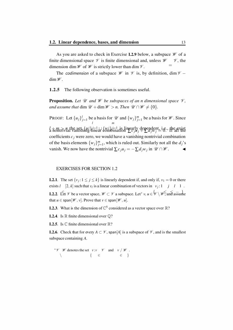
As you are asked to check in Exercise I.2.9 below, a subspace W of a
finite dimensional space V is finite dimensional and, unless W =V , the
dimension dimW of W is strictly lower than dimV .
The codimension of a subspace W in V is, by definition, dimV −dimW .
1.2.5 The following observation is sometimes useful.
Proposition. Let U and W be subspaces of an n dimensional space V ,
and assume that dimU + dimW > n. Then U ∩W = {0}.
PROOF: Let {u j}l j=1 be a basis for U and {w j}m
j=1 be a basis forW . Since
l + m > n the set {u j}l
j=1 ∪ {w j}m
j=1 is linearly dependent, i.e., the exista nontrivial vanishing linear combination ∑c ju j +∑d jw j = 0. If all the
coefficients c j were zero, we would have a vanishing nontrivial combination
of the basis elements {w j}m j=1, which is ruled out. Similarly not all the d j’s
vanish. We now have the nontrivial ∑c ju j = −∑d jw j in U ∩W .
EXERCISES FOR SECTION 1.2
I.2.1. The set {v j : 1 ≤ j ≤ k } is linearly dependent if, and only if, v1 = 0 or there
exists l
∈[2, k ] such that vl is a linear combination of vectors in
{v j : 1
≤j
≤l
−1
}.
I.2.2. Let V be a vector space,W ⊂ V a subspace. Let∗ v, u ∈V \W , and assume
that u ∈ span[W , v]. Prove that v ∈ span[W , u].
I.2.3. What is the dimension of C5 considered as a vector space over R?
I.2.4. Is R finite dimensional over Q?
I.2.5. Is C finite dimensional over R?
I.2.6. Check that for every A ⊂ V , span[ A] is a subspace of V , and is the smallest
subspace containing A.
∗V \W denotes the set
{v : v
∈V and v /
∈W
}.

7/27/2019 katznelson-linalgebra
http://slidepdf.com/reader/full/katznelson-linalgebra 20/185
14 I. Vector spaces
I.2.7. Let U , W be subspaces of a vector space V , and assume U ∩W = {0}.
Assume that{
u1
, . . . ,uk } ⊂
U and{
w1
, . . . ,wl} ⊂
W are (each) linearly indepen-
dent. Prove that {u1, . . . ,uk }∪{w1, . . . ,wl} is linearly independent.
I.2.8. Prove that the subspacesW j ⊂ V , j = 1, . . . , N are independent (see Defini-
tion 1.1.4) if, and only if, W j ∩∑l= jW l = {0} for all j.
I.2.9. Let V be finite dimensional. Prove that every subspace W ⊂ V is finite
dimensional, and that dimW ≤ dimV with equality only if W = V .
I.2.10. If V is finite dimensional, every subspace W ⊂ V is a direct summand.
∗I.2.11. Assume that V is n-dimensional vector space over an infinite F. Let {W j}be a finite collection of distinct m-dimensional subspaces.
a. Prove that no W j is contained in the union of the others.
b. Prove that there is a subspace U ⊂ V which is a complement of every W j.Hint: See exercise I.1.6.
I.2.12. Let V andW be finite dimensional subspaces of a vector space. Prove that
V +W and V ∩W are finite dimensional and that
(1.2.1) dim(V ∩W ) + dim(V +W ) = dimV + dimW .
I.2.13. If W j, j = 1, . . . ,k , are finite dimensional subspaces of a vector space V
then∑W j is finite dimensional and dim∑W j ≤∑dimW j, with equality if, and only
if, the subspaces W j are independent.
I.2.14. Let V be an n-dimensional vector space, and let V 1⊂V be a subspace of
dimension m.
a. Prove that V /V 1—the quotient space—is finite dimensional.
b. Let {v1, . . . ,vm} be a basis for V 1 and let {w1, . . . ,wk } be a basis for V /V 1.
For j ∈ [1, k ], let w j be an element of the coset w j.
Prove: {v1, . . . ,vm}∪{w1, . . . ,wk } is a basis for V . Hence k + m = n.
I.2.15. Let V be a real vector space. Let r l = (al,1, . . . ,al, p) ∈ R p, 1 ≤ l ≤ s be
linearly independent. Let v1, . . . ,v p ∈ V be linearly independent. Prove that the
vectors ul =∑ p1 al, jv j, l = 1, . . . ,s, are linearly independent in V .
I.2.16. Let V and U be finite dimensional spaces over F. Prove that the tensor
productV
⊗U is finite dimensional. Specifically, show that if
{e j
}n j=1 and
{ f k
}mk =1

7/27/2019 katznelson-linalgebra
http://slidepdf.com/reader/full/katznelson-linalgebra 21/185
1.3. Systems of linear equations. 15
are bases for V and U , then {e j ⊗ f k }, 1 ≤ j ≤ n, 1 ≤ k ≤ m, is a basis forV ⊗U ,so that dimV
⊗U = dimV dimU .
∗I.2.17. Assume that any three of the fiveR3 vectors v j = ( x j, y j, z j), j = 1, . . . , 5,
are linearly independent. Prove that the vectors
w j = ( x2 j , y2
j , z2 j , x j y j, x j z j, y j z j)
are linearly independent in R6.
Hint: Find non-zero (a, b, c) such that ax j + by j + cz j = 0 for j = 1, 2. Find
non-zero (d , e, f ) such that dx j + ey j + f z j = 0 for j = 3, 4. Observe (and use) the
fact
(ax5 + by5 + cz5)(dx5 + ey5 + f z5) = 0
1.3 Systems of linear equations.
How do we find out if a set {v j}, j = 1, . . . , m of column vectors in
Fnc is linearly dependent? How do we find out if a vector u belongs to
span[v1...,vm]?
Given the vectors v j =
a1 j
.
..
an j
, j = 1, . . . , m, and and u =
c1
.
..
cn
, we ex-
press the conditions ∑ x jv j = 0 for the first question, and ∑ x jv j = u for the
second, in terms of the coordinates.
For the first we obtain the system of homogeneous linear equations:
(1.3.1)
a11 x1 + . . . + a1m xm = 0
a21 x1 + . . . + a2m xm = 0...
...
an1 x1 + . . . + anm xm = 0
or,
(1.3.2)m
∑ j=1
ai j x j = 0, i = 1, . . . , n.

7/27/2019 katznelson-linalgebra
http://slidepdf.com/reader/full/katznelson-linalgebra 22/185
16 I. Vector spaces
For the second question we obtain the non-homogeneous system:
(1.3.3)m
∑ j=1
ai j x j = ci, i = 1, . . . , n.
We need to determine if the solution-set of the system (1.3.2), namely
the set of all m-tuples ( x1, . . . , xm) ∈ Fm for which all n equations hold, is
trivial or not, i.e., if there are solutions other than (0, . . . , 0). For (1.3.3) we
need to know if the solution-set is empty or not. In both cases we would like
to identify the solution set as completely and as explicitely as possible.
1.3.1 Conversely, given the system (1.3.2) we can rewrite it as
(1.3.4) x1
a11...
an1
+ · · · + xm
a1m...
anm
= 0
Our first result depends only on dimension. The m vectors in (1.3.4) are
elements of the n-dimensional space Fnc . If m > n, any m vectors in Fn
c
are dependent, and since we have a nontrivial solution if, and only if, these
columns are dependent, the system has nontrivial solution. This proves the
following theorem.
Theorem. A system of n homogeneous linear equations in m > n unknowns
has nontrivial solutions.
Similarly, rewriting (1.3.3) in the form
(1.3.5) x1
a11
..
.
an1
+ · · ·+ xm
a1m
..
.
anm
=
c1
..
.
cn
,
it is clear that the system given by (1.3.3) has a solution if, and only if, the
column
c1
.
..
cn
is in the span of columns
a1 j
.
..
an j
, j ∈ [1, m].

7/27/2019 katznelson-linalgebra
http://slidepdf.com/reader/full/katznelson-linalgebra 23/185
1.3. Systems of linear equations. 17
1.3.2 The classical approach to solving systems of linear equations is the
Gaussian elimination— an algorithm for replacing the given system by an
equivalent system that can be solved easily. We need some terminology:
DEFINITION: The systems
(A)m
∑ j=1
ai j x j = ci, i = 1, . . . , k .
(B)m
∑ j=1
bi j x j = d i, i = 1, . . . , l.
(1.3.6)
are equivalent if they have the same solution-set (in Fm).
The matrices
A =
a11 . . . a1m
a21 . . . a2m
... . . ....
ak 1 . . . akm
and Aaug =
a11 . . . a1m c1
a21 . . . a2m c2
... . . ....
...
ak 1 . . . akm ck
are called the matrix and the augmented matrix of the system (A). The
augmented matrix is obtained from the matrix by adding, as additional col-
umn, the column of the values, that is, the right-hand side of the respective
equations. The augmented matrix contains all the information of the system
(A). Any k × (m + 1) matrix is the augmented matrix of a system of linear
equations in m unknowns.
1.3. 3 ROW EQUIVALENCE OF MATRICES.
DEFINITION: The matrices
(1.3.7)
a11 . . . a1m
a21 . . . a2m
... . . ....
ak 1 . . . akm
and
b11 . . . b1m
b21 . . . b2m
... . . ....
bl1 . . . blm
are row equivalent if their rows span the same subspace of Fm
r ; equivalently:
if each row of either matrix is a linear combination of the rows of the other.

7/27/2019 katznelson-linalgebra
http://slidepdf.com/reader/full/katznelson-linalgebra 24/185
18 I. Vector spaces
Proposition. Two systems of linear equations in m unknowns
(A)m
∑ j=1
ai j x j = ci, i = 1, . . . , k .
(B)m
∑ j=1
bi j x j = d i, i = 1, . . . , l.
are equivalent if their respective augmented matrices are row equivalent.
PROOF: Assume that the augmented matrices are row equivalent.
If ( x1, . . . , xm) is a solution for system (A) and
(bi1, . . . , bim, d i) =∑α i,k (ak 1, . . . , akm, ck )
thenm
∑ j=1
bi j x j =∑k , j
α i,k ak j x j =∑k
α i,k ck = d i
and ( x1, . . . , xm) is a solution for system (B).
DEFINITION: The row rank of a matrix A ∈M (k , m) is the dimension of
the span of its rows in Fm.
Row equivalent matrices clearly have the same rank.
1.3 .4 REDUCTION TO ROW ECHELON FORM . The classical method
of solving systems of linear equations, homogeneous or not, is the Gaussianelimination. It is an algorithm to replace the system at hand by an equivalent
system that is easier to solve.
DEFINITION: A matrix A =
a11 . . . a1m
a21 . . . a2m
... . . ....
ak 1 . . . akm
is in (reduced) row echelon
form if the following conditions are satisfied
ref –1 The first q rows of A are linearly independent in Fm, the remaining
k
−q rows are zero.

7/27/2019 katznelson-linalgebra
http://slidepdf.com/reader/full/katznelson-linalgebra 25/185
1.3. Systems of linear equations. 19
ref –2 There are integers 1 ≤ l1 < l2 < · · · < lq ≤ m such that for j ≤ q, the
first nonzero entry in the j’th row is 1, occuring in the l j
’th column.
ref –3 The entry 1 in row j is the only nonzero entry in the l j column.
One can rephrase the last three conditions as: The l j’th columns (the
“main” columns) are the first q elements of the standard basis of Fk c, and ev-
ery other column is a linear combination of the “main” columns that precede
it.
Theorem. Every matrix is row equivalent to a matrix in row-echelon form.
PROOF: If A = 0 there’s nothing to prove. Assuming A = 0, we describe an
algorithm to reduce A to row-echelon form. The operations performed onthe matrix are:
a. Reordering (i.e., permuting) the rows,
b. Multiplying a row by a non-zero constant,
c. Adding a multiple of one row to another.
These operations do not change the span of the rows so that the equivalence
class of the matrix is maintained. (We shall return later, in Exercise II.3.10,
to express these operations as matrix multiplications.)
Let l1 be the index of the first column that is not zero.
Reorder the rows so that a1,l1= 0, and multiply the first row by a−1
1,l1.
Subtract from the j’th row, j = 1, the first row multiplied by a j,l1 .Now all the columns before l1 are zero and column l1 has 1 in the first
row, and zero elswhere.
Denote its row rank of A by q. If q = 1 all the entries below the first
row are now zero and we are done. Otherwise let l2 be the index of the first
column that has a nonzero entry in a row beyond the first. Notice that l2 > l1.
Keep the first row in its place, reorder the remaining rows so that a2,l2= 0,
and multiply the second row∗ by a−12,l2
.
Subtruct from the j’th row, j = 2, the second row multiplied by a j,l2.
∗We keep referring to the entries of the successively modified matrix as ai j.

7/27/2019 katznelson-linalgebra
http://slidepdf.com/reader/full/katznelson-linalgebra 26/185
20 I. Vector spaces
Repeat the sequence a total of q times. The first q rows, r1, . . . , rq, are
(now) independent: a combination ∑c j
r j
has entry c j
in the l j
’th place, and
can be zero only if c j = 0 for all j.
If there is a nonzero entry beyond the current q’th row, necessarily be-
yond the lq’th column, we could continue and get a row independent of the
first q, contradicting the definition of q. Thus, after q steps, all the rows
beyond the q’th are zero.
Observe that the scalars used in the process belong to the smallest field
that contains all the coefficients of A.
1.3.5 If A and Aaug are the matrix and the augmented matrix of a system
(A) and we apply the algorithm of the previous subsection to both, we ob-
serve that since the augmented matrix has the additional column on the right
hand side, the first q (the row rank of A) steps in the algorithm for either A or
Aaug are identical. Having done q repetitions, A is reduced to row-echelon
form, while Aaug may or may not be. If the row rank of Aaug is q, then the
algorithm for Aaug ends as well; otherwise we have lq+1 = m + 1, and the
row-echelon form for the augmented matrix is the same as that of A but with
an added row and an added “main” column, both having 0 for all but the last
entries, and 1 for the last entry. In the latter case, the system corresponding
to the row-reduced augmented matrix has as it last equation 0 = 1 and the
system has no solutions.
On the other hand, if the row rank of the augmented matrix is the same as
that of A, the row-echelon form of the augmented matrix is an augmentation
of the row-echelon form of A. In this case we can assign arbitrary values
to the variables xi, i = l j, j = 1, . . . , q, move the corresponding terms to the
right hand side and, writing C j for the sum, we obtain
(1.3.8) xl j= C j, j = 1, . . . , q.
Theorem. A necessary and sufficient condition for the system (A) to have
solutions is that the row rank of the augmented matrix be equal to that of
the matrix of the system.

7/27/2019 katznelson-linalgebra
http://slidepdf.com/reader/full/katznelson-linalgebra 27/185
1.3. Systems of linear equations. 21
The discussion preceding the statement of the theorem not only proves
the theorem but offers a concrete way to solve the system. The unknowns are
now split into two groups, q “main” ones and m − q “secondary”. We have
“m − q degrees of freedom”: the m − q secondary unknowns become free
parameters that can be assigned arbitrary values, and these values determine
the “main” unknowns uniquely.
Remark: Notice that the split into “main” and “secondary” unknowns de-
pends on the specific definition of “row–echelon form”; counting the columns
in a different order may result in a different split, though the number q of
“main” variables would be the same—the row rank of A.
Corollary. A linear system of n equations in n unknowns with matrix A has
solutions for all augmented matrices if, and only if, the only solution of the
corresponding homogeneous system is the trivial solution.
PROOF: The condition on the homogeneous system amounts to “the rows
of A are independent”, and no added columns can increase the row rank.
1.3.6 DEFINITION: The column rank of a matrix A ∈ M (k , m) is the
dimension of the span of its columns in Fk c.
Linear relations between columns of A are solutions of the homogeneous
system given by A. If B is row-equivalent to A, the columns of A and B have
the same set of linear relations, (see Proposition 1.3.3). In particular, if B isin row-echelon form and {l j}q
j=1 are the indices of the “main” columns in
B, then the l j’th columns in A, j = 1, . . . , q, are independent, and every other
column is a linear combination of these.
It follows that the column rank of A is equal to its row rank. We shall
refer to the common value simply as the rank of A.
———–
The span of the rows stays the same.
The span of the columns changes, the rank stays the same
The annihilator (solution set) stays (almost) the same.
————-

7/27/2019 katznelson-linalgebra
http://slidepdf.com/reader/full/katznelson-linalgebra 28/185
22 I. Vector spaces
EXERCISES FOR SECTION 1.3
I.3.1. Identify the matrix A ∈M (n) of row rank n that is in row echelon form.
I.3.2. A system of linear equations with rational coefficients, that has a solution in
C, has a solution in Q. Equivalently, vectors inQn that are linearly dependent over
C, are rationally dependent.
Hint: The last sentence of Subsection 1.3.4.
I.3.3. A system of linear equations with rational coefficients, has the same number
of “degrees of freedom” over Q as it does over C.
I.3.4. An affine subspace of a vector space is a translate of a subspace, that is a set
of the form v0 +V 0 = {v0 + v : v ∈ V 0}, where v0 is a fixed vector and V 0 ⊂ V is a
subspace. (Thus a line in V is a translate of a one-dimensional subspace.)Prove that a set A ⊂ V is an affine subspace if, and only if, ∑a ju j ∈ A for all
choices of u1, . . . , uk ∈ A, and scalars a j, j = 1, . . . ,k such that ∑a j = 1.
I.3.5. If A ⊂ V is an affine subspace and u0 ∈ A, then A − u0 = {u − u0 : u ∈ A}is a subspace of V . Moreover, the subspace A − u0, the “corresponding subspace”
does not depend on the choice of u0.
I.3.6. The solution set of a system of k linear equations in m unknowns is an affine
subspace of Fm. The solution set of the corresponding homogeneous system is the
“corresponding subspace”.
I.3.7. Consider the matrix A =
a11 . . . a1ma21 . . . a2m
... . . ....
ak 1 . . . akm
and its columns v j =
a1 j
..
.
ak j
.
Prove that a column vi ends up as a “main column” in the row echelon form of A
if, and only if, it is linearly independent of the columns v j, j < i.
I.3.8. (continuation) Denote by B =
b11 . . . b1m
b21 . . . b2m
... . . ....
bk 1 . . . bkm
the matrix in row echelon
form obtained from A by the algorithm described above. Let l1 < l2, . . . be the

7/27/2019 katznelson-linalgebra
http://slidepdf.com/reader/full/katznelson-linalgebra 29/185
1.3. Systems of linear equations. 23
indices of the main columns in B and i the index of another column. Prove
(1.3.9) vi = ∑l j<i
b jivl j.
I.3.9. What is the row echelon form of the 7× 6 matrix A, if its columns C j, j =
1, . . . ,6 satisfy the following conditions:
a. C 1 = 0;
b. C 2 = 3C 1;
c. C 3 is not a (scalar) multiple of C 1;
d. C 4 = C 1 + 2C 2 + 3C 3;
e. C 5 = 6C 3;
f. C 6 is not in the span of C 2 and C 3.
∗I.3.10. Given polynomials P1 = ∑n0 a j x
j, P2 = ∑m0 b j x
j, anbm = 0,S = ∑l0 s j x
j
of degrees n, m, and l < n + m respectively, we want to find polynomials q1 =
∑m−10 c j x
j, and q2 =∑n−10 d j x
j, such that
(1.3.10) P1q1 + P2q2 = S .
Allowing the leading coefficients of S to be zero, there is no loss of generality in
writing S =∑m+n−10 s j x
j.
The polynomial equation (1.3.10) is equivalent to a system of m + n linear
equations, the unknown being the coefficients cm−1, . . . ,c0 of q1, and d n−1, . . . ,d 0
of q2.
(1.3.11) ∑ j+k =l
a jck + ∑r +t =l
br d t = sl l = 0, . . . ,n + m − 1
If we write a j = 0 for j > n and for j < 0, and write b j = 0 for j > m and for j < 0,
so that (formally) P1 = ∑∞−∞a j x
j, P2 = ∑∞−∞ b j x
j, then the matrix of our system ist i j
where,
(1.3.12) t i j =
an+ j−i for 1 ≤ j ≤ n,
bm
−n+ j
−i for 1
≤n < j
≤n + m,

7/27/2019 katznelson-linalgebra
http://slidepdf.com/reader/full/katznelson-linalgebra 30/185
24 I. Vector spaces
The matrix of this system is
(1.3.13)
an 0 0 0 . . . 0 0 0
an−1 an 0 0 . . . 0 0 0
an−2 an−1 an 0 0 . . . 0 0...
......
......
......
...
a0 a1 a2 a3 . . . . . . . . .
0 a0 a1 a2 a3 . .. . ..
0 0 a0 a1 a2 a3 . . .
0 0 0 a0 a1 a2 a3 . . .
0 0 0 0 0 0
0 0 0 0 0 0
0 0 0 0 0 0
.
(1.3.14)
an an−1 an−2 . . . a0 0 0 0 . . . 0
0 an an−1 an−2 . . . a0 0 0 . . . 0
0 0 an an−1 an−2 . . . a0 0 . . . 0...
......
......
......
......
...
0 . . . . . . 0 an an−1 an−2 . . . a1 a0
bm bm−1 bm−2 . . . b0 0 0 0 . . . 0
0 bm bm−1 bm−2 . . . b0 0 0 . . . 0
0 0 bm bm−1 bm−2 . . . b0 0 . . . 0...
......
......
......
......
...
0 . . . . . . 0 bm bm−1 bm−2 . . . b1 b0
.
The determinant† of the matrix of the system is called the resultant of the pair
P1, P2
∗I.3.11. The associated homogeneous system corresponds to the case S = 0. Show
that it has a nontrivial solutions if, and only if, P1 and P2 have a nontrivial common
factor. (You may assume the unique factorization theorem, A.6.3.)
What is the rank of the resultant matrix if the degree of gcd(P1, P2) is r .
†See Chapter IV.

7/27/2019 katznelson-linalgebra
http://slidepdf.com/reader/full/katznelson-linalgebra 31/185
1.3. Systems of linear equations. 25
———————————————-
Define “degrees of freedom”
Discuss uniqueness of the row echelon form

7/27/2019 katznelson-linalgebra
http://slidepdf.com/reader/full/katznelson-linalgebra 32/185
26 I. Vector spaces

7/27/2019 katznelson-linalgebra
http://slidepdf.com/reader/full/katznelson-linalgebra 33/185
Chapter II
Linear operators and matrices
2.1 Linear Operators (maps, transformations)
2.1.1 Let V and W be vector spaces over the same field.
DEFINITION: A map T : V → W is linear if for all vectors v j ∈ V and
scalars a j,
(2.1.1) T (a1v1 + a2v2) = a1T v1 + a2T v2.
This was discussed briefly in 1.1.2. Linear maps are also called linear oper-
ators, linear transformations, homomorphisms, etc. The adjective “linear”
is sometimes assumed implicitly. The term we use most of the time is oper-
ator .
EXAMPLES:
a. The identity map I of V onto itself, defined by Iv = v for all v ∈ V .
b. If {v1, . . . , vn} is a basis for V and {w1, . . . , wn} ⊂W is arbitrary, thenthe map v j → w j, j = 1, . . . , n extends (uniquely) to a linear map T from
V to W defined by
(2.1.2) T : ∑a jv j →∑a jw j.
Every linear operator from V into W is obtained this way.
c. Let V be the space of all continuous, 2π -periodic functions on the line.
For every x0 define T x0, the translation by x0:
T x0: f ( x)
→f x0
( x) = f ( x
− x0).
27

7/27/2019 katznelson-linalgebra
http://slidepdf.com/reader/full/katznelson-linalgebra 34/185
28 II. Linear operators and matrices
d. The transpose .
(2.1.3) A =
a11 . . . a1m
a21 . . . a2m
... . . ....
an1 . . . anm
→ ATr
=
a11 . . . an1
a12 . . . an2
... . . ....
a1m . . . anm
which maps M (n, m;F) onto M (m, n;F).
e. Differentiation on F[ x]:
(2.1.4) D :n
∑0
a j x j →
n
∑1
ja j x j−1.
The definition is purely formal, involves no limiting process, and is validfor arbitrary field F.
f. Differentiation on T N :
(2.1.5) D : N
∑− N
aneinx → N
∑− N
in aneinx.
There is no formal need for a limiting process: D is defined by (2.1.5).
g. Differentiation on C ∞[0, 1], the complex vector space of infinitely dif-
ferentiable complex-valued functions on [0, 1]:
(2.1.6) D : f → f = d f dx
.
h. If V = W ⊕ U every v ∈ V has a unique representation v = w + u
with w ∈ W , u ∈ U . The map π 1 : v → w is the identity on W and
maps U to {0}. It is called the projection of V on W along U .
The operator π 1 is linear since, if v = w + u and v1 = w1 + u1, then
av + bv1 = (aw + bw1) + (au + bu1), and π 1(av + bv1) = aπ 1v + bπ 1v1.
Similarly, π 2 : v → u is called the projection of V on U along W . π 1and π 2 are referred to as the projections corresponding to the direct
sum decomposion.

7/27/2019 katznelson-linalgebra
http://slidepdf.com/reader/full/katznelson-linalgebra 35/185
2.1. Linear Operators (maps, transformations) 29
2.1.2 We denote the space of all linear maps fromV intoW byL (V ,W ).
Another common notation is HOM (V
,W
). The two most important cases
in what follows are: W = V , and W = F, the field of scalars.
When W = V we write L (V ) instead of L (V ,V ).
When W is the underlying field, we refer to the linear maps as linear
functionals or linear forms on V . Instead of L (V ,F) we write V ∗, and
refer to it as the dual space of V .
2.1.3 If T ∈L (V ,W ) is bijective, it is invertible, and the inverse map
T −1 is linear from W onto V . This is seen as follows: by (2.1.1),
T −1(a1T v1 + a2T v2) =T −1(T (a1v1 + a2v2)) = a1v1 + a2v2
= a1T −1
(T v1) + a2T −1
(T v2),
(2.1.7)
and, as T is surjective, T v j are arbitrary vectors in W .
Recall (see 1.1.2) that an isomorphism of vector spaces, V and W is a
bijective linear map T : V →W . An isomorphism of a space onto itself is
called an automorphism.
V and W are isomorphic if there is an isomorphism of the one onto
the other. The relation is clearly reflexive and, by the previous paragraph,
symmetric. Since the concatenation (see 2.2.1) of isomorphisms is an iso-
morphism, the relation is also transitive and so is an equivalence relation.
The image of a basis under an isomorphism is a basis, see exercise II.1.2; it
follows that the dimension is an isomorphism invariant.
If V is a finite dimensional vector space overF, every basis v = {v1, . . . , vn}of V defines an isomorphism Cv of V onto Fn by:
(2.1.8) Cv : v =∑a jv j →a1
.
..
an
=∑a je j.
Cv v is the coordinate vector of v relative to the basis v. Notice that this
is a special case of example a. above: we map the basis elements v j on the
corresponding elements e j of the standard basis, and extend by linearity.

7/27/2019 katznelson-linalgebra
http://slidepdf.com/reader/full/katznelson-linalgebra 36/185
30 II. Linear operators and matrices
If V and W are both n-dimensional, with bases v = {v1, . . . , vn}, and
w= {
w1, . . . ,
wn}
respectively, the map T : ∑a j
v j →
∑a j
w j
is an isomor-
phism. This shows that the dimension is a complete invariant : finite di-
mensional vector spaces over F are isomorphic if, and only if, they have the
same dimension.
2.1.4 The sum of linear maps T , S ∈ L (V ,W ), and the multiple of a
linear map by a scalar are defined by: for every v ∈ V ,
(2.1.9) (T + S )v = T v + Sv, (aT )v = a(T v).
Observe that (T + S ) and aT , as defined, are linear maps from V to W , i.e.,
elements of L (V ,W ).
Proposition. Let V and W be vector spaces over F. Then, with the addi-
tion and multiplication by a scalar defined by (2.1.9) , L (V ,W ) is a vector
space defined over F. If both V and W are finite dimensional, then so is
L (V ,W ) , and dimL (V ,W ) = dimV dimW .
PROOF: The proof that L (V ,W ) is a vector space over F is straightfor-
ward checking, left to the reader.
The statement about the dimension is exercise II.1.3 below.
EXERCISES FOR SECTION 2.1
II.1.1. Show that if a set A ⊂ V is linearly dependent and T ∈L (V ,W ), then TA
is linearly dependent in W .
II.1.2. Prove that an injective map T ∈L (V ,W ) is an isomorphism if, and only
if, it maps some basis of V onto a basis of W , and this is the case if, and only if, it
maps every basis of V onto a basis of W .
II.1.3. Let V and W be finite dimensional with bases v = {v1, . . . ,vn} and
w = {w1, . . . ,wm} respectively. Let ϕ i j ∈L (V ,W ) be defined by ϕ i jvi = w j and
ϕ i j vk = 0 for k = i. Prove that {ϕ i j : 1 ≤ i ≤ n, 1 ≤ j ≤ m} is a basis forL (V ,W ).

7/27/2019 katznelson-linalgebra
http://slidepdf.com/reader/full/katznelson-linalgebra 37/185
2.2. Operator Multiplication 31
2.2 Operator Multiplication
2.2.1 For T ∈L (V ,W ) and S ∈L (W ,U ) we define ST ∈L (V ,U )by concatenation, that is: (ST )v = S (T v). ST is a linear operator since
(2.2.1) ST (a1v1 + a2v2) = S (a1T v1 + a2T v2) = a1ST v1 + a2ST v2.
In particular, if V =W = U , we have T , S , and T S all in L (V ).
Proposition. With the product ST defined above,L (V ) is an algebra over
F.
PROOF: The claim is that the product is associative and, with the addition
defined by (2.1.9) above, distributive. This is straightforward checking, left
to the reader.
The algebra L (V ) is not commutative unless dimV = 1, in which
case it is simply the underlying field.
The set of automorphisms, i.e., invertible elements in L (V ) is a group
under multiplication, denoted GL(V ).
2.2.2 Given an operator T ∈L (V ) the powers T j of T are well defined
for all j ≥ 1, and we define T 0 = I . Since we can take linear combinations
of the powers of T we have P(T ) well defined for all polynomials P ∈ F[ x];
specifically, if P( x) = ∑a j x
j
then P(T ) = ∑a jT
j
.We denote
(2.2.2) P (T ) = {P(T ) : P ∈ F[ x]}.
P (T ) will be the main tool in understanding the way in which T acts on V .
EXERCISES FOR SECTION 2.2
II.2.1. Give an example of operators T , S ∈L (R2) such that T S = ST .
Hint: Let e1, e2 be a basis for R2, define T by Te1 = Te2 = e1 and define S by
Se1 = Se2 = e2.

7/27/2019 katznelson-linalgebra
http://slidepdf.com/reader/full/katznelson-linalgebra 38/185
32 II. Linear operators and matrices
II.2.2. Prove that, for any T ∈ L (V ), P (T ) is a commutative subalgebra of
L (V ).
II.2.3. For T ∈L (V ) denote comm[T ] = {S : S ∈L (V ), ST = T S }, the set of
operators that commute with T . Prove that comm[T ] is a subalgebra of L (V ).
II.2.4. Verify that GL(V ) is in fact a group.
II.2.5. An element π ∈L (V ) is idempotent if π 2 = π . Prove that an idempotent
π is a projection onto π V (its range), along {v :π v = 0} (its kernel).
——————— John Erdos: every singular operator is a product of
idempotents
(as exercises later)
—————————
2.3 Matrix multiplication.
2.3.1 We define the product of a 1 × n matrix (row) r = (a1, . . . , an) and
an n × 1 matrix (column) c =
b1
...
bn
, to be the scalar given by
(2.3.1) r · c =∑a jb j,
Given A ∈M (l, m) and B ∈M (m, n), we define the product AB as the
l ×n matrix C whose entries ci j are given by
(2.3.2) ci j = ri( A) · c j( B) =∑k
aik bk j
(ri( A) denotes the i’th row in A, and c j( B) denotes the j’th column in B).
Notice that the product is defined only when the number of columns in
A (the length of the row) is the same as the number of rows in B, (the height
of the column).
The product is associative: given A ∈ M (l, m), B ∈ M (m, n), and
C ∈ M (n, p), then AB ∈ M (l, n) and ( AB)C ∈ M (l, p) is well defined.
Similarly, A( BC ) is well defined and one checks that A( BC ) = ( AB)C by
verifying that the r , s entry in either is ∑i, j ar jb jicis.

7/27/2019 katznelson-linalgebra
http://slidepdf.com/reader/full/katznelson-linalgebra 39/185
2.3. Matrix multiplication. 33
The product is distributive: for A j ∈M (l, m), B j ∈M (m, n),
(2.3.3) ( A1 + A2)( B1 + B2) = A1 B1 + A1 B2 + A2 B1 + A2 B2,
and commutes with multiplication by scalars: (aA) B = A(aB) = a( AB).
Proposition. The map ( A, B) → AB, of M (l, m) ×M (m, n) to M (l, n) , is
linear in B for every fixed A, and in A for every fixed B.
PROOF: The statement just summarizes the properties of the multiplication
discussed above.
2.3.2 Write the n × m matrix
ai j
1≤i≤n
1≤ j≤m
as a “single column of rows”,
a11 . . . a1m
a21 . . . a2m
... . . ....
an1 . . . anm
=a11 . . . a1ma21 . . . a2m
...an1 . . . anm
=
r1
r2
...
rn
where ri =
ai,1 . . . ai,m
∈ Fm
r . Notice that if x1, . . . , xn
∈ Fnr , then
(2.3.4) x1, . . . , xn
a11 . . . a1m
a21 . . . a2m
... . . ....
an1 . . . anm
= x1, . . . , xn
r1
r2
...
rn
=n
∑i=1
xiri.
Similarly, writing the matrix as a “single row of columns”,a11 . . . a1m
a21 . . . a2m
... . . ....
an1 . . . anm
=
a11
a21
...
an1
a12
a22
...
an2
. . .
a1m
a2m
...
anm
=
c1, c2, . . . ,cm
we have
(2.3.5)
a11 . . . a1m
a21 . . . a2m
... . . ....
an1 . . . anm
y1
y2
...
ym
=
c1, c2, . . . ,cm
y1
y2
...
ym
=m
∑ j=1
y jc j.

7/27/2019 katznelson-linalgebra
http://slidepdf.com/reader/full/katznelson-linalgebra 40/185
34 II. Linear operators and matrices
2.3.3 If l = m = n matrix multiplication is a product withinM (n).
Proposition. With the multiplication defined above, M (n) is an algebra
over F. The matrix I = I n = (δ j,k ) = ∑n1 eii is the identity∗ element inM (n).
The invertible elements in M (n), aka the non-singular matrices, form a
group under multiplication, the general linear group GL(n,F).
Theorem. A matrix A ∈M (n) is invertible if, and only if its rank is n.
PROOF: Exercise II.3.2 below (or equation (2.3.4)) give that the row rank
of BA is no bigger than the row rank of A. If BA = I , the row rank of A is at
least the row rank of I , which is clearly n.
On the other hand, if A is row equivalent to I , then its row echelon formis I , and by Exercise II.3.10 below, reduction to row echelon form amounts
to multiplication on the left by a matrix, so that A has a left inverse. This
implies, see Exercise II.3.12, that A is invertible.
EXERCISES FOR SECTION 2.3
II.3.1. Let r be the 1 × n matrix all whose entries are 1, and c the n × 1 matrix all
whose entries are 1. Compute rc and cr.
II.3.2. Prove that each of the columns of the matrix AB is a linear combinations
of the columns of A, and that each row of AB is a linear combination of the rows of
B.
II.3.3. A square matrix (ai j) is diagonal if the entries off the diagonal are all zero,
i.e., i = j =⇒ ai j = 0.
Prove: If A is a diagonal matrix with distinct entries on the diagonal, and if B
is a matrix such that AB = BA, then B is diagonal.
II.3.4. Denote by Ξ(n; i, j), 1 ≤ i, j ≤ n, the n × n matrix ∑k =i, j ekk + ei j + e ji (the
entries ξlk are all zero except for ξi j = ξ ji = 1, and ξkk = 1 if k = i, j. This is the
matrix obtained from the identity by interchanging rows i and j.
∗δ j,k is the Kronecker delta, equal to 1 if j = k , and to 0 otherwise.

7/27/2019 katznelson-linalgebra
http://slidepdf.com/reader/full/katznelson-linalgebra 41/185
2.3. Matrix multiplication. 35
Let A ∈M (n, m) and B ∈M (m, n). Describe Ξ(n; i, j) A and BΞ(n; i, j).
II.3.5. Let σ be a permutation of [1, . . . ,n]. Let Aσ be the n × n matrix whoseentries ai j are defined by
(2.3.6) ai j =
1 if i = σ ( j)
0 otherwise.
Let B ∈M (n, m) and C ∈M (m, n). Describe Aσ B and CAσ .
II.3.6. A matrix whose entries are either zero or one, with precisely one non-zero
entry in each row and in each column is called a permutation matrix . Show that
the matrix Aσ described in the previous exercise is a permutation matrix and that
every permutation matrix is equal to Aσ for some σ ∈ Sn.
II.3.7. Show that the map σ
→ Aσ defined above is multiplicative: Aστ = Aσ Aτ .
(στ is defined by concatenation: στ ( j) = σ (τ ( j)) for all j ∈ [1, n].)
II.3.8. Denote by ei j, 1 ≤ i, j ≤ n, the n×n matrix whose entries are all zero except
for the i j entry which is 1. With A ∈M (n, m) and B ∈M (m, n). Describe ei j A and
Bei j.
II.3.9. Describe an n × n matrix A(c, i, j) such that multiplying on the appropriate
side, an n×n matrix B by it, has the effect of replacing the i’th row in B by the sum
of the i’th row and c times the j’th row. Do the same for columns.
II.3.10. Show that each of the steps in the reduction of a matrix A to its row-echelon
form (see 1.3.4) can be accomplished by left multiplication of A by an appropriate
matrix, so that the entire reduction to row-echelon form can be accomplished by left
multiplication by an appropriate matrix. Conclude that if the row rank of A ∈M (n)
is n, then A is left-invertible.
II.3.11. Let A ∈M (n) be non-singular and let B = ( A, I ), the matrix obtained
by “augmenting” A by the identity matrix, that is by adding to A the columns of
I in their given order as columns n + 1, . . . ,2n. Show that the matrix obtained by
reducing B to row echelon form is ( I , A−1).
II.3.12. Prove that if A ∈M (n, m) and B ∈M (m, l) then† ( AB)Tr
= BTr
ATr
. Show
that if A ∈M (n) has a left inverse then ATr
has a right inverse and if A has a right
†For the notation, see 2.1, example d.

7/27/2019 katznelson-linalgebra
http://slidepdf.com/reader/full/katznelson-linalgebra 42/185
36 II. Linear operators and matrices
inverse then ATr
has a left inverse. Use the fact that A and ATr
have the same rank
to show that if A has a left inverse B it also has a right inverse C and since B =
B( AC ) = ( BA)C = C , we have BA = AB = I and A has an inverse.
Where does the fact that we deal with finite dimensional spaces enter the
proof?
II.3.13. What are the ranks and the inverses (when they exist) of the matrices
(2.3.7)
0 2 1 0
1 1 7 1
2 2 2 2
0 5 0 0
,
1 1 1 1 1
0 2 2 1 1
2 1 2 1 2
0 5 0 9 1
0 5 0 0 7
,
1 1 1 1 1
0 1 1 1 1
0 0 1 1 1
0 0 0 1 1
0 0 0 0 1
.
II.3.14. Denote An = 1 n0 1 . Prove that Am An = Am+n for all integers m, n.
II.3.15. Let A, B,C , D ∈M (n) and let E =
A B
C D
∈M (2n) be the matrix whose
top left quarter is a copy of A, the top right quarter a copy of B, etc.
Prove that E 2 =
A2 + BC AB + BD
CA + DC CB + D2.
2.4 Matrices and operators.
2.4.1 Recall that we write the elements of Fn as columns. A matrix A
in M (m, n) defines, by multiplication on the left, an operator T A from Fn
to Fm. The columns of A are the images, under T A, of the standard basisvectors of Fn (see (2.3.5)).
Conversly, given T ∈ L (Fn,Fm), if we take A = AT to be the m × n
matrix whose columns are Te j, where {e1, . . . , en} is the standard basis in
Fn, we have T A = T .
Finally we observe that by Proposition 2.3.1 the map A → T A is linear.
This proves:
Theorem. There is a 1-1 linear correspondence T ↔ AT betweenL (Fn,Fm)
and M (m, n) such that T ∈L (Fn,Fm) is obtained as a left multiplication
by the m
×n matrix, AT .

7/27/2019 katznelson-linalgebra
http://slidepdf.com/reader/full/katznelson-linalgebra 43/185
2.4. Matrices and operators. 37
2.4.2 If T ∈L (Fn,Fm) and S ∈L (Fm,Fl) and AT ∈M (m, n), resp. AS ∈M
(l,
m)
are the corresponding matrices, then
ST ∈L (Fn,Fl), AS AT ∈M (l, n), and AST = AS AT .
In particular, if n = m = l, we obtain
Theorem. The map T ↔ AT is an algebra isomorphism between L (Fn)
and M (n).
2.4.3 The special thing about Fn is that it has a “standard basis”. The
correspondence T ↔ AT (or A ↔ T A) uses the standard basis implicitly.
Consider now general finite dimensional vector spaces V and W . Let
T ∈ L (V ,W ) and let v = {v1, . . . , vn} be a basis for V . As mentioned
earlier, the images {T v1, . . . , T vn} of the basis elements determine T com-pletely. In fact, expanding any vector v ∈ V as v = ∑c jv j, we must have
T v = ∑c jT v j.
On the other hand, given any vectors y j ∈W , j = 1, . . . , n we obtain an
element T ∈L (V ,W ) by declaring that T v j = y j for j = 1, . . . , n, and (nec-
essarily) T (∑a jv j) = ∑a j y j. Thus, the choice of a basis in V determines
a 1-1 correspondence between the elements of L (V ,W ) and n-tuples of
vectors in W .
2.4.4 If w = {w1, . . . , wm} is a basis for W , and T v j = ∑mk =1 t k , jwk , then,
for any vector v =∑c jv j, we have
(2.4.1) T v =∑c jT v j =∑ j∑
k
c jt k , jwk =∑k
∑
j
c jt k , j
wk .
Given the bases {v1, . . . , vn} and {w1, . . . , wm}, the full information about T
is contained in the matrix
(2.4.2) AT ,v,w =
t 11 . . . t 1n
t 21 . . . t 2n
... . . ....
t m1 . . . t mn
= (Cw T v1, . . . ,Cw T vn).

7/27/2019 katznelson-linalgebra
http://slidepdf.com/reader/full/katznelson-linalgebra 44/185
38 II. Linear operators and matrices
The “coordinates operators”, Cw, assign to each vector inW the column of
its coordinates with respect to the basis w, see (2.1.8).
When W = V and w = v we write AT ,v instead of AT ,v,v.
Given the bases v and w, and the matrix AT ,v,w, the operator T is explic-
itly defined by (2.4.1) or equivalently by
(2.4.3) Cw T v = AT ,v,wCv v.
Let A ∈M (m, n), and denote by Sv the vector inW whose coordinates with
respect to w are given by the column ACv v. So defined, S is clearly a linear
operator in L (V ,W ) and AS ,v,w = A. This gives:
Theorem. Given the vector spaces V and W with bases v = {v1, . . . , vn}and w = {w1, . . . , wm} repectively, the map T → AT ,v,w is a bijection of L (V ,W ) onto M (m, n).
2.4 .5 CHANGE OF BASIS. Assume now that W = V , and that v and w
are arbitrary bases. The v-coordinates of a vector v are given by Cv v and the
w-coordinates of v by Cw v. If we are given the v-coordinates of a vector v,
say x = Cv v, and we need the w-coordinates of v, we observe that v = C-1v x,
and hence Cw v = CwC-1v x. In other words, the operator
(2.4.4) Cw,v = CwC-1v
on Fn assigns to the v-coordinates of a vector v
∈V its w-coordinates. The
factor C-1v identifies the vector from its v-coordinates, and Cw assigns to the
identified vector its w-coordinates; the space V remains in the background.
Notice that C-1v,w = Cw,v
Suppose that we have the matrix AT ,w of an operator T ∈L (V ) relative
to a basis w, and we need to have the matrix AT ,v of the same operator
T , but relative to a basis v. (Much of the work in linear algebra revolves
around finding a basis relative to which the matrix of a given operator is as
simple as possible—a simple matrix is one that sheds light on the structure,
or properties, of the operator.) Claim:
(2.4.5) AT ,v = Cv,w AT ,wCw,v,

7/27/2019 katznelson-linalgebra
http://slidepdf.com/reader/full/katznelson-linalgebra 45/185
2.4. Matrices and operators. 39
Cw,v assigns to the v-coordinates of a vector v ∈ V its w-coordinates; AT ,w
replaces the w-coordinates of v by those of T v; Cv,w
identifies T v from its
w-coordinates, and produces its v-coordinates.
2.4.6 How special are the matrices (operators) Cw,v? They are clearly
non-singular, and that is a complete characterization.
Proposition. Given a basis w = {w1, . . . , wn} of V , the map v → C w,v is a
bijection of the set of bases v of V onto GL(n,F).
PROOF: Injectivity: Since Cw is non-singular, the equality Cw,v1= Cw,v2
implies C-1v1
= C-1v2
, and since C-1v1
maps the elements of the standard basis of
Fn onto the corresponding elements in v1, and C-1v2
maps the same vectors
onto the corresponding elements in v2, we have v1 = v2.
Surjectivity: Let S ∈ GL(n,F) be arbitrary. We shall exhibit a base v
such that S = Cw,v. By definition, Cw w j = e j, (recall that {e1, . . . , en} is the
standard basis for Fn). Define the vectors v j by the condition: Cw v j = Se j,
that is, v j is the vector whose w-coordinates are given by the j’th column of
S . As S is non-singular the v j’s are linearly independent, hence form a basis
v of V .
For all j we have v j = C-1v e j and Cw,v e j = Cw v j = Se j. This proves that
S = Cw,v
2.4. 7 SIMILARITY. The matrices B1 and B2 are said to be similar if they
represent the same operator T in terms of (possibly) different bases, that is, B1 = AT ,v and B2 = AT ,w.
If B1 and B2 are similar, they are related by (2.4.5). By Proposition 2.4.6
we have
Proposition. The matrices B1 and B2 are similar if, and only if there exists
C ∈ GL(n,F) such that
(2.4.6) B1 = CB2C −1.
We shall see later (see exercise V.6.4) that if there exists such C with
entries in some field extension of F, then one exists in M (n,F).
A matrix is diagonalizable if it is similar to a diagonal matrix.

7/27/2019 katznelson-linalgebra
http://slidepdf.com/reader/full/katznelson-linalgebra 46/185
40 II. Linear operators and matrices
2.4.8 The operators S , T ∈ L (V ) are said to be similar if there is an
operator R∈
GL(V
)such that
(2.4.7) T = RSR−1.
An operator is diagonalizable if its matrix is. Notice that the matrix AT ,v of
T relative to a basis v = {v1, . . . , vn} is diagonal if, and only if, T vi = λ ivi,
where λ i is the i’th entry on the diagonal of AT ,v.
EXERCISES FOR SECTION 2.4
II.4.1. Prove that S , T ∈L (V ) are similar if, and only if, their matrices (relative
to any basis) are similar. An equivalent condition is: for any basis w there is a basis
v such that AT ,v = AS ,w.
II.4.2. Let Fn[ x] be the space of polynomials ∑n0 a j x
j. Let D be the differentiation
operator and T = 2 D + I .
a. What is the matrix corresponding to T relative to the basis { x j}n j=0?
b. Verify that, if u j = ∑nl= j x
l , then {u j}n j=0 is a basis, and find the matrix
corresponding to T relative to this basis.
II.4.3. Prove that if A ∈M (l, m), the map T : B → AB is a linear operatorM (m, n) →M (l, n). In particular, if n = 1,M (m, 1) =Fm
c andM (l, 1) =Flc and T ∈L (Fm
c ,Flc).
What is the relation between A and the matrix AT defined in 2.4.3 (for the standard
bases, and with n there replaced here by l)?
2.5 Kernel, range, nullity, and rank
2.5.1 DEFINITION: The kernel of an operator T ∈L (V ,W ) is the set
ker(T ) = {v ∈ V : T v = 0}.
The range of T is the set
range(T ) = T V = {w ∈W : w = T v for some v ∈ V }.
The kernel is also called the nullspace of T .

7/27/2019 katznelson-linalgebra
http://slidepdf.com/reader/full/katznelson-linalgebra 47/185
2.5. Kernel, range, nullity, and rank 41
Proposition. Assume T ∈L (V ,W ). Then ker(T ) is a subspace of V , and
range(
T )
is a subspace of W .
PROOF: If v1, v2 ∈ ker(T ) then T (a1v1 + a2v2) = a1T v1 + a2T v2 = 0.
If v j = Tu j then a1v1 + a2v2 = T (a1u1 + a2u2).
If V is finite dimensional and T ∈ L (V ,W ) then both ker(T ) and
range(T ) are finite dimensional; the first since it is a subspace of a finite
dimensional space, the second as the image of one, (since, if {v1, . . . , vn} is
a basis for V , {T v1, . . . , T vn} spans range(T )).
We define the rank of T , denoted ρ(T), as the dimension of range(T ).
We define the nullity of T , denoted ν (T), as the dimension of ker(T ).
Theorem ( Rank and nullity). Assume T ∈L (V ,W ) , V finite dimensional.
(2.5.1) ρ(T) +ν (T) = dimV .
PROOF: Let {v1, . . . , vl} be a basis for ker(T ), l = ν (T), and extend it to
a basis of V by adding {u1, . . . , uk }. By 1.2.4 we have l + k = dimV .
The theorem follows if we show that k = ρ(T). We do it by showing that
{Tu1, . . . , Tuk } is a basis for range(T ).
Write any v ∈ V as ∑li=1 aivi +∑k
i=1 biui. Since T vi = 0, we have T v =
∑k i=1 biTui, which shows that {Tu1, . . . , Tuk } spans range(T ).
We claim that {Tu1, . . . , Tuk } is also independent. To show this, assumethat ∑
k j=1 c jTu j = 0, then T
∑
k j=1 c ju j
= 0, that is ∑
k j=1 c ju j ∈ ker(T ).
Since {v1, . . . , vl} is a basis for ker(T ), we have ∑k j=1 c ju j = ∑
l j=1 d jv j for
appropriate constants d j. But {v1, . . . , vl}∪{u1, . . . , uk } is independent, and
we obtain c j = 0 for all j.
The proof gives more than is claimed in the theorem. It shows that T can
be “factored” as a product of two maps. The first is the quotient map V →V /ker(T ); vectors that are congruent modulo ker(T ) have the same image
under T . The second, V /ker(T ) → TV is an isomorphism. (This is the
Homomorphism Theorem of groups in our context.)

7/27/2019 katznelson-linalgebra
http://slidepdf.com/reader/full/katznelson-linalgebra 48/185
42 II. Linear operators and matrices
2.5.2 The identity operator, defined by Iv = v, is an identity element in the
algebra L (V
). The invertible elements in L
(V
)are the
automorphisms of V , that is, the bijective linear maps. In the context of finite dimensional
spaces, either injectivity (i.e. being 1-1) or surjectivity (onto) implies the
other:
Theorem. Let V be a finite dimensional vector space, T ∈LV . Then
(2.5.2) ker(T ) = {0} ⇐⇒ range(T ) = V ,
and either condition is equivalent to: “T is invertible”, aka “nonsingular”.
PROOF: ker(T ) = {0} is equivalent to ν (T) = 0, and range(T ) = V is
equivalent to ρ(T) = dimV . Now apply (2.5.1).
2.5.3 As another illustration of how the “rank and nullity” theorem can
be used, consider the following statment (which can be seen directly as a
consequence of exercise I.2.12)
Theorem. Let V = V 1 ⊕V 2 be finite dimensional, dimV 1 = k. Let W ⊂ V be a subspace of dimension l > k. Then dimW ∩V 2 ≥ l − k.
PROOF: Denote by π 1 the restriction to W of the projection of V on V 1
along V 2. Since the rank of π 1 is clearly ≤ k , the nullity is ≥ l −k . In other
words, the kernel of this map, namely W ∩V 2, has dimension ≥ l − k .
EXERCISES FOR SECTION 2.5
II.5.1. Assume T , S ∈L (V ). Prove that ν (ST) ≤ ν (S) +ν (T) .
II.5.2. Give an example of two 2× 2 matrices A and B such that ρ(AB) = 1 and
ρ(BA) = 0.
II.5.3. Given vector spaces V and W over the same field. Let {v j}n j=1 ⊂ V and
{w j}n j=1 ⊂W . Prove that there exists a linear map T : span[v1, . . . ,vn] →W such
that T v j = w j, j = 1, . . . ,n if, and only if, the following implication holds:
If a j, j = 1 . . . ,n are scalars, andn
∑1
a jv j = 0, thenn
∑1
a jw j = 0.

7/27/2019 katznelson-linalgebra
http://slidepdf.com/reader/full/katznelson-linalgebra 49/185
2.5. Kernel, range, nullity, and rank 43
Can the definition of T be extended to the entire V ?
II.5.4. What is the relationship of the previous exercise to Theorem 1.3.5?II.5.5. The operators T , S ∈L (V ) are called “equivalent” if there exist invertible
A, B ∈L (V ) such that
S = ATB (so that T = A−1SB−1).
Prove that if V is finite dimensional then T , S are “equivalent” if, and only if
ρ(S) = ρ(T) .
II.5.6. Give an example of two operators onF3 that are equivalent but not similar.
II.5.7. Assume T , S ∈L (V ). Prove that the following statements are equivalent:
a. ker(S ) ⊂ ker(T ),
b. There exists R ∈L (V ) such that T = RS .
Hint: For the implication a.=⇒b.: Choose a basis {v1, . . . ,vs} for ker(S ). Expand
it to a basis for ker(T ) by adding {u1, . . . ,ut −s}, and expand further to a basis for
V by adding the vectors {w1, . . . ,wn−t }.
The sequence {Su1, . . . ,Sut −s}∪{Sw1, . . . ,Swn−t } is independent, so that R can
be defined arbitrarily on it (and extended by linearity to an operator on the entire
space). Define R(Su j) = 0, R(Sw j) = Tw j.
The other implication is obvious.
II.5.8. Assume T , S ∈L (V ). Prove that the following statements are equivalent:
a. range(S ) ⊂ range(T ),
b. There exists R ∈L (V ) such that S = T R.
Hint: Again, b. =⇒ a. is obvious.
For a. =⇒ b. Take a basis {v1, . . . ,vn} for V . Let u j, j = 1, . . . ,n be such that
Tu j = Sv j, (use assumption a.). Define Rv j = u j (and extend by linearity).
II.5.9. Find bases for the null space, ker( A), and for the range, range( A), of the
matrix (acting on rows in R5)
1 0 0 5 9
0 1 0 −3 2
0 0 1 2 1
3 2 1 11 32
1 2 0
−1 13
.

7/27/2019 katznelson-linalgebra
http://slidepdf.com/reader/full/katznelson-linalgebra 50/185
44 II. Linear operators and matrices
II.5.10. Let T ∈L (V ), l ∈N. Prove:
a. ker(T l ) ⊆ ker(T l+1); equality if, and only if range(T l ) ∩ker(T ) = {0}.
b. range(T l+1) ⊆ range(T l ); equality if, and only if, ker(T l+1) = ker(T l ).
c. If ker(T l+1) = ker(T l), then ker(T l+k +1) = ker(T l+k ) for all positive integers
k .
II.5.11. An operator T is idempotent if T 2 = T . Prove that an idempotent operator
is a projection on range(T ) along ker(T ).
∗II.5.12. The rank of a skew-symmetric matrix is even.
2.6 Normed finite dimensional linear spaces
2.6.1 A norm on a real or complex vector space V is a nonnegative func-
tion v → v that satisfies the conditions
a. Positivity: 0 = 0 and if v = 0 then v > 0.
b. Homogeneity: av = |a|v for scalars a and vectors v.
c. The triangle inequality: v + u ≤ v+ u.
These properties guarantee that ρ(v, u) =
v
−u
is a metric on the
space, and with a metric one can use tools and notions from point-set topol-ogy such as limits, continuity, convergence, infinite series, etc.
A vector space endowed with a norm is a normed vector space .
2.6.2 If V and W are isomorphic real or complex n-dimensional spaces
and S is an isomorphism of V onto W , then a norm ·∗ on W can be
transported to V by defining v = Sv∗. This implies that all possible
norms on a real n-dimensional space are copies of norms on Rn, and all
norms on a complex n-dimensional space are copies of norms on Cn.
A finite dimensional V can be endowed with many different norms; yet,
all these norms are equivalent in the following sense:

7/27/2019 katznelson-linalgebra
http://slidepdf.com/reader/full/katznelson-linalgebra 51/185
2.6. Normed finite dimensional linear spaces 45
DEFINITION: The norms ·1 and ·2 are equivalent, written: ·1 ∼·2
if there is a positive constant C such that for all v∈V
C −1v1 ≤ v2 ≤ C v1
The metrics ρ1, ρ2, defined by equivalent norms, are equivalent: for v, u ∈V
C −1ρ1(v, u) ≤ ρ2(v, u) ≤ C ρ1(v, u).
which means that they define the same topology—the familiar topology of
Rn or Cn.
2.6.3 If V andW are normed vector spaces we define a norm onL (V ,W )
by writing, for T ∈L (V ,W ),
(2.6.1) T = maxv=1
T v = maxv=0
T vv .
Equivalently,
(2.6.2) T = inf {C :T v ≤ C v for all v ∈H }.
To check that (2.6.1) defines a norm we observe that properties a. and b. are
obvious, and that c. follows from∗
(T + S )v
≤ T v
+
Sv
≤ T
v
+
S
v
≤(
T
+
S
)
v
.
L (V ) is an algebra and we observe that the norm defined by (2.6.1)
on L (V ) is submultiplicative : we have ST v ≤ S T v ≤ S T v,
where S , T ∈L (V ) and v ∈ V , which means
(2.6.3) ST ≤ S T .
EXERCISES FOR SECTION 2.6
∗Notice that the norms appearing in the inequalities are the ones defined on W ,
L (V ,W ), and V , respectively.

7/27/2019 katznelson-linalgebra
http://slidepdf.com/reader/full/katznelson-linalgebra 52/185
46 II. Linear operators and matrices
II.6.1. Let V be n-dimensional real or complex vector space, v = {v1, . . . ,vn} a
basis for V . Write
∑a jv j
v,1 =∑
|a j
|, and
∑a jv j
v,∞ = max
|a j
|.
Prove:
a. ·v,1 and ·v,∞ are norms on V , and
(2.6.4) ·v,∞ ≤·v,1 ≤ n·v,∞
b. If · is any norm on V then, for all v ∈ V ,
(2.6.5) vv,1 maxv j ≥ v.
II.6.2. Let · j, j = 1, 2, be norms on V , and ρ j the induced metrics. Let {vn}∞n=0
be a sequence in V and assume that ρ1(vn, v0) → 0. Prove ρ2(vn, v0) → 0.II.6.3. Let {vn}∞n=0 be bounded in V . Prove that ∑
∞0 vn z
n converges for every z
such that | z| < 1.
Hint: Prove that the partial sums form a Cauchy sequence in the metric defined by
the norm.
II.6.4. Let V be n-dimensional real or complex normed vector space. The unit
ball in V is the set
B1 = {v ∈ V :v ≤ 1}.
Prove that B1 is
a. convex : If v, u ∈ B1, 0 ≤ a ≤ 1, then av + (1 − a)u ∈ B1.
b. Bounded: For every v
∈V , there exist a (positive) constant λ such that
cv /∈ B for |c| > λ .
c. Symmetric, centered at 0: If v ∈ B and |a| ≤ 1 then av ∈ B.
II.6.5. Let V be n-dimensional real or complex vector space, and let B be a
bounded symmetric convex set centered at 0. Define
u = inf {a > 0 : a−1u ∈ B}.
Prove that this defines a norm on V , and the unit ball for this norm is the given
B
II.6.6. Describe a norm 0 on R3 such that the standard unit vectors have norm
1 while
(1, 1, 1)
0 < 1
100.

7/27/2019 katznelson-linalgebra
http://slidepdf.com/reader/full/katznelson-linalgebra 53/185
2.6. Normed finite dimensional linear spaces 47
II.6.7. Let V be a normed linear space and T ∈ L (V ). Prove that the set of
vectors v∈V whose T -orbit,
{T nv
}, is bounded is a subspace of V .
ADDITIONAL EXERCISES FOR CHAPTER II
II.+.1. Projections — idempotents.
Theorem ( Erdos). Every non-invertible element of L (V ) is a product of projec-
tions.
II.+.2.

7/27/2019 katznelson-linalgebra
http://slidepdf.com/reader/full/katznelson-linalgebra 54/185
48 II. Linear operators and matrices

7/27/2019 katznelson-linalgebra
http://slidepdf.com/reader/full/katznelson-linalgebra 55/185
Chapter III
Duality of vector spaces
3.1 Linear functionals
DEFINITION: A linear functional , a.k.a linear form, on a vector space V
is a linear map of V into F, the underlying field.
—————-Add a remark to the effect that, unless stated explicitly otherwise, the
vector spaces we consider are assumed to be finite dimensional.
————–
Let V be a finite dimensional vector space with basis {v1, . . . , vn}. Every
element v ∈ V can be written, in exactly one way, as
(3.1.1) v =n
∑1
a j(v)v j,
the notation a j(v) comes to emphasize the dependence of the coefficients on
the vector v.Let v =∑
n1 a j(v)v j, and u =∑
n1 a j(u)v j. If c, d ∈ F, then
cv + du =n
∑1
(ca j(v) + da j(u))v j
so that
a j(cv + du) = ca j(v) + da j(u).
In other words, a j(v) are linear functionals on V .
A standard notation for the image of a vector v under a linear functional
v∗ is (v, v∗). Accordingly we denote the linear functionals corresponding to
49

7/27/2019 katznelson-linalgebra
http://slidepdf.com/reader/full/katznelson-linalgebra 56/185
50 III. Duality of vector spaces
a j(v) by v∗ j and write
(3.1.2) a j(v) = (v, v∗ j ) so that v =
n∑
1
(v, v∗ j )v j.
Proposition. The linear functionals v∗ j , j = 1, . . . , n form a basis for the
dual space V ∗.
PROOF: Let u∗ ∈ V ∗. Write b j(u∗) = (v j, u∗), then for any v ∈ V ,(v, u∗) = (∑
j
(v, v∗ j )v j, u∗) =∑
j
(v, v∗ j )b j(u∗) = (v,∑b j(u∗)v∗
j ),
and u∗ = ∑b j(u∗)v∗ j . It follows that {v∗
1, . . . , v∗n} spans V ∗. On the other
hand,
{v∗
1, . . . , v∗n
}is independent since ∑c jv∗
j = 0 implies (vk ,∑c jv∗ j ) =
ck = 0 for all k .
Corollary. dimV ∗ = dimV .
The basis {v∗ j}n
1, j = 1, . . . , n is called the dual basis of {v1, . . . , vn}. It
is characterized by the condition
(3.1.3) (v j, v∗k ) = δ j,k ,
δ j,k is the Kronecker delta, it takes the value 1 if j = k , and 0 otherwise.
3.1.1 The way we add linear functionals or multiply them by scalars guar-
antees that the form (expression) (v, v∗), v
∈V and v∗
∈V ∗, is bilinear , that
is linear in v for every fixed v∗, and linear in v∗ for any fixed v. Thus every
v ∈ V defines a linear functional on V ∗.
If {v1, . . . , vn} is a basis forV , and {v∗1, . . . , v∗
n} the dual basis inV ∗, then
(3.1.3) identifies {v1, . . . , vn} as the dual basis of {v∗1, . . . , v∗
n}. The roles of V
and V ∗ are perfectly symmetric and what we have is two spaces in duality ,
the duality between them defined by the bilinear form (v, v∗). (3.1.2) works
in both directions, thus if {v1, . . . , vn} and {v∗1, . . . , v∗
n} are dual bases, then
for all v ∈ V and v∗ ∈ V ∗,
(3.1.4) v =n
∑1
(v, v∗ j )v j, v∗ =
n
∑1
(v j, v∗)v∗ j .

7/27/2019 katznelson-linalgebra
http://slidepdf.com/reader/full/katznelson-linalgebra 57/185
3.1. Linear functionals 51
The dual of Fnc (i.e., Fn written as columns) can be identified with Fn
r
(i.e.,
F
n written as rows) and the pairing(
v,
v∗)
as the matrix product v∗
v
of the row v∗ by the column v, (exercise III.1.4 below). The dual of the
standard basis of Fnc is the standard basis Fn
r .
3.1. 2 ANNIHILATOR. Given a set A ⊂ V , the set of all the linear func-
tionals v∗ ∈ V ∗ that vanish identically on A is called the annihilator of A
and denoted A⊥. Clearly, A⊥ is a subspace of V ∗.
Functionals that annihilate A vanish on span[ A] as well, and functionals
that annihilate span[ A] clearly vanish on A; hence A⊥ = (span[ A])⊥.
Proposition. Let V 1 ⊂ V be a subspace, then dimV 1 + dimV ⊥1 = dimV .
PROOF: Let {v1, . . . , vm} be a basis for V 1, and let {vm+1, . . . , vn} complete
it to a basis for V . Let {v∗1, . . . , v∗
n} be the dual basis.
We claim, that {v∗m+1, . . . , v∗
n} is a basis for V ⊥1 ; hence dimV ⊥1 = n − m
proving the proposition.
By (3.1.3) we have {v∗m+1, . . . , v∗
n} ⊂ V ⊥1 , and we know these vectors to
be independent. We only need to prove that they span V ⊥1 .
Let w∗ ∈ V ⊥1 , Write w∗ = ∑n j=1 a jv∗
j , and observe that a j = (v j, w∗).
Now w∗
∈V ⊥1 implies a j = 0 for 1
≤j
≤m, so that w∗ = ∑
nm+1 a jv∗
j .
Theorem. Let A ⊂ V , v ∈ V and assume that (v, u∗) = 0 for every u∗ ∈ A⊥.
Then v ∈ span[ A].
Equivalent statement: If v /∈ span[ A] then there exists u∗ ∈ A⊥ such that
(v, u∗) = 0.
PROOF: If v /∈ span[ A], then dim span[ A, v] = dim span[ A] + 1, and hence
dim span[ A, v]⊥ = dim span[ A]⊥ −1. It follows that span[ A]⊥ span[ A, v]⊥,
and since functionals in A⊥ which annihilate v annihilate span[ A, v], there
exist functionals in A⊥ that do not annihilate v.
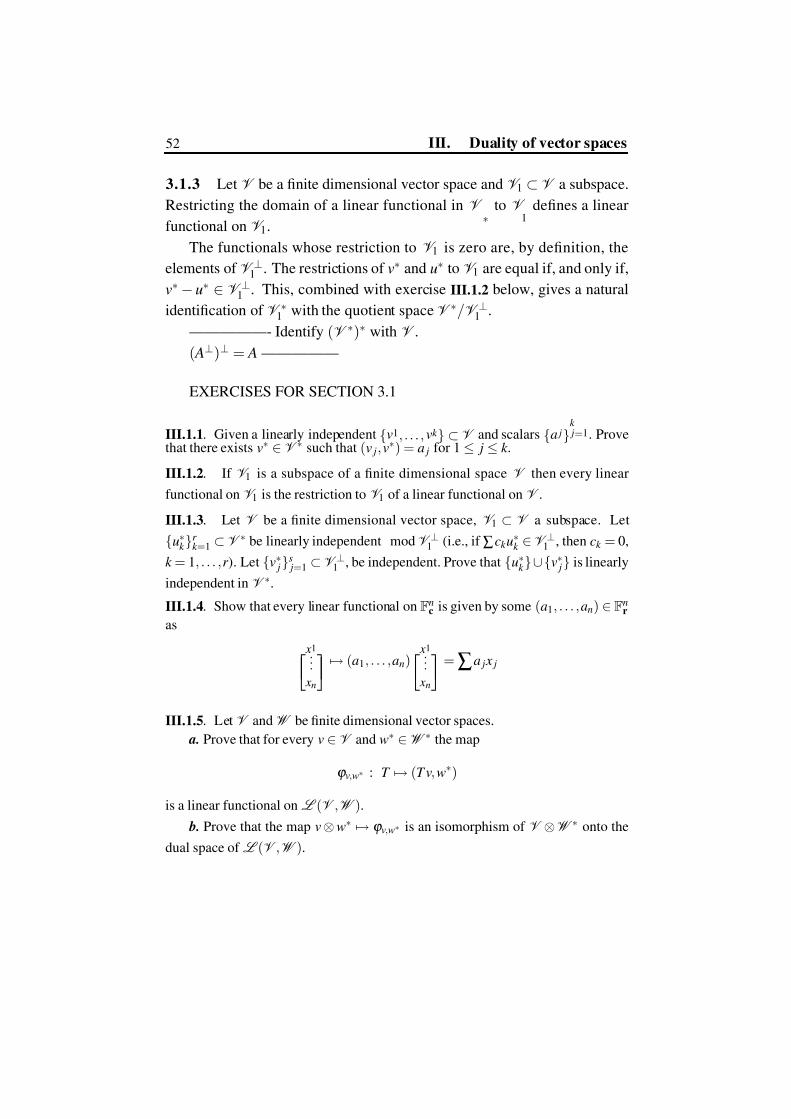
7/27/2019 katznelson-linalgebra
http://slidepdf.com/reader/full/katznelson-linalgebra 58/185
52 III. Duality of vector spaces
3.1.3 Let V be a finite dimensional vector space and V 1 ⊂ V a subspace.
Restricting the domain of a linear functional in V ∗
to V 1
defines a linear
functional on V 1.
The functionals whose restriction to V 1 is zero are, by definition, the
elements of V ⊥1 . The restrictions of v∗ and u∗ to V 1 are equal if, and only if,
v∗ − u∗ ∈ V ⊥1 . This, combined with exercise III.1.2 below, gives a natural
identification of V ∗1 with the quotient space V ∗/V ⊥1 .
—————- Identify (V ∗)∗ with V .
( A⊥)⊥ = A —————
EXERCISES FOR SECTION 3.1
III.1.1. Given a linearly independent {v1, . . . , vk } ⊂ V and scalars {a j}k j=1. Prove
that there exists v∗ ∈ V ∗ such that (v j, v∗) = a j for 1 ≤ j ≤ k .
III.1.2. If V 1 is a subspace of a finite dimensional space V then every linear
functional on V 1 is the restriction to V 1 of a linear functional on V .
III.1.3. Let V be a finite dimensional vector space, V 1 ⊂ V a subspace. Let
{u∗k }r
k =1 ⊂ V ∗ be linearly independent mod V ⊥1 (i.e., if ∑ck u∗k ∈V ⊥1 , then ck = 0,
k = 1, . . . ,r ). Let {v∗ j}s
j=1 ⊂V ⊥1 , be independent. Prove that {u∗k }∪{v∗
j} is linearly
independent in V ∗.
III.1.4. Show that every linear functional on Fnc is given by some (a1, . . . ,an) ∈ Fn
r
as x1...
xn
→ (a1, . . . ,an) x1
..
.
xn
=∑a j x j
III.1.5. Let V andW be finite dimensional vector spaces.
a. Prove that for every v ∈ V and w∗ ∈W ∗ the map
ϕ v,w∗ : T → (T v, w∗)
is a linear functional on L (V ,W ).
b. Prove that the map v ⊗ w∗ → ϕ v,w∗ is an isomorphism of V ⊗W ∗ onto the
dual space of L (V ,W ).

7/27/2019 katznelson-linalgebra
http://slidepdf.com/reader/full/katznelson-linalgebra 59/185
3.2. The adjoint 53
III.1.6. Let V be a complex vector space, {v∗ j}s
j=1 ⊂ V ∗, and w∗ ∈ V ∗ such that
for all v
∈V ,
|v, w∗| ≤ maxs j=1|v, v∗
j|.
Prove that w∗ ∈ span[{v∗ j}s
j=1].
III.1.7. Linear functionals on R N [ x]:
1. Show that for every x ∈ R the map ϕ x defined by (P,ϕ x) = P( x) is a linear
functional on R N [ x].
2. If { x1, . . . , xm} are distinct and m ≤ N + 1, then ϕ x jare linearly independent.
3. For every x
∈R and l
∈N, l
≤ N , the map ϕ
(l) x defined by (P,ϕ
(l) x ) = P(l)( x)
is a (non-trivial) linear functional on R N [ x].
——————
P(l)( x) denotes the l’th derivative of P at x.
———————
III.1.8. Let x j ∈R, l j ∈N, and assume that the pairs ( x j, l j), j = 1, . . . , N + 1, are
distinct. Denote by #(m) the number of such pairs with l j > m.
a. Prove that a necessary condition for the functionals ϕ (l j)
x jto be independent on
R N [ x] is:
(3.1.5) for every m ≤ N , #(m) ≤ N − m.
b. Check that ϕ 1, ϕ −1, and ϕ (1)0 are linearly dependent in the dual of R2[ x], hence
(3.1.5) is not sufficient. Are ϕ 1, ϕ −1, and ϕ (1)0 linearly dependent in the dual of
R3[ x]?
3.2 The adjoint
——————-
Here or put off till Inner Product spaces?
——————–

7/27/2019 katznelson-linalgebra
http://slidepdf.com/reader/full/katznelson-linalgebra 60/185
54 III. Duality of vector spaces
3.2.1 The concatenation w∗T of T ∈L (V ,W ), and w∗ ∈W ∗, is a linear
map from V to the underlying field, i.e. a linear functional v∗
on V .
With T fixed, the mapping w∗ → w∗T is a linear operator T ∗ ∈L (W ∗,V ∗).
It is called the adjoint of T .
The basic relationship between T , T ∗, and the bilinear forms (v, v∗) and
(w, w∗) is: For all v ∈ V and w∗ ∈W ∗,
(3.2.1) (T v, w∗) = (v, T ∗w∗).
Notice that the left-hand side is the bilinear form on (W ,W ∗), while the
right-hand side in (V ,V ∗).
3.2.2 Proposition.
(3.2.2) ρ(T*) = ρ(T) .
PROOF: Let T ∈ L (V ,W ), assume ρ(T) = r , and let {v1, . . . , vn} be a
basis for V such that {vr +1, . . . , vn} is a basis for ker(T ). We have seen
(see the proof of theorem 2.5.1) that {T v1, . . . , T vr } is a basis for T V =
range(T ).
Denote w j = T v j, j = 1, . . . , r . Add the vectors w j, j = r + 1, . . . , m so
that {w1, . . . , wm} be a basis for W . Let {w∗1, . . . , w∗
m} be the dual basis.
Fix k > r ; for every j ≤ r we have (v j, T ∗w∗k ) = (w j, w∗
k ) = 0 which
means T ∗w∗k = 0. Thus T ∗W ∗ is spanned by {T ∗w∗
j}r j=1.
For 1 ≤ i, j ≤ r , (vi, T ∗w∗ j ) = (wi, w∗ j ) =δ i, j, which implies that {T ∗w∗ j}r
j=1is linearly independent in V ∗.
Thus, {T ∗w∗1, . . . , T ∗w∗
r } is a basis for T ∗W ∗, and ρ(T*) = ρ(T).
3.2.3 We have seen in 3.1.1 that if V = Fnc , W = Fm
c , both with standard
bases, then V ∗ = Fnr , W ∗ = Fm
r , and the standard basis of Fmr is the dual
basis of the standard basis of Fnc .
If A = AT =
t 11 . . . t 1n
... . . ....
t m1 . . . t mn
, is the matrix of T with respect to the standard
bases, then the operator T is given as left multiplication by A on Fnc and the

7/27/2019 katznelson-linalgebra
http://slidepdf.com/reader/full/katznelson-linalgebra 61/185
3.2. The adjoint 55
bilinear form (T v, w), for w ∈ Fmr and v ∈ Fn
c , is just the matrix product
(3.2.3) w( Av) = (wA)v.
It follows that T ∗w = wAT , that is, the action of T ∗ on the row vectors in Fmr
is obtained as multiplication on the right by the same matrix A = AT .
If we want∗ to have the matrix of T ∗ relative to the standard bases in
Fnc and Fm
c , acting on columns by left multiplication, all we need to do is
transpose wA and obtain
T ∗wTr
= ATr
wTr
.
3.2.4 Proposition. Let T ∈L (V ,W ). Then
(3.2.4) range(T )⊥ = ker(T ∗) and range(T ∗)⊥ = ker(T ).
PROOF: w∗ ∈ range(T )⊥ is equivalent to (T v, w∗) = (v, T ∗w∗) = 0 for all
v ∈ V , and (v, T ∗w∗) = 0 for all v ∈ V is equivalent to T ∗w∗ = 0.
The condition v ∈ range(T ∗)⊥ is equivalent to (v, T ∗w∗) = 0 for all
w∗ ∈ W ∗, and T v = 0 is equivalent to (T v, w∗) = (v, T ∗w∗) = 0 i.e. v ∈range(T ∗)⊥.
EXERCISES FOR SECTION 3.2
III.2.1. If V =W ⊕ U and S is the projection of V on W along U (see
2.1.1.h), what is the adjoint S ∗?III.2.2. Let A ∈M (m, n;R). Prove
ρ(ATr
A) = ρ(A)
III.2.3. Prove that, in the notation of 3.2.2, {w∗ j} j=r +1,...,m is a basis for
ker(T ∗).
∗This will be the case when there is a natural way to identify the vector space with
its dual, for instance when we work with inner product spaces . If the “identification” is
sesquilinear, as is the case when F= C the matrix for the adjoint is the complex conjugate
of ATr
, , see Chapter VI.

7/27/2019 katznelson-linalgebra
http://slidepdf.com/reader/full/katznelson-linalgebra 62/185
56 III. Duality of vector spaces
III.2.4. A vector v ∈ V is an eigenvector for T ∈L (V ) if T v = λ v with
λ ∈ F
; λ is the correspondingeigenvalue
.
Let v ∈ V be an eigenvector of T with eigenvalue λ , and w ∈ V ∗ an
eigenvector of the adjoint T ∗ with eigenvalue λ ∗ = λ . Prove that (v, w∗) =
0.
7/27/2019 katznelson-linalgebra
http://slidepdf.com/reader/full/katznelson-linalgebra 63/185
Chapter IV
Determinants
4.1 Permutations
A permutation of a set is a bijective, that is 1-1, map of the set onto
itself. The set of permutations of the set [1, . . . , n] is denoted Sn. It is a group
under concatenation—given σ ,τ ∈ Sn define τσ by (τσ )( j) = τ (σ ( j)) forall j. The identity element of Sn is the trivial permutation e defined by
e( j) = j for all j.
Sn with this operation is called the symmetric group on [1, . . . , n].
4.1.1 If σ ∈ Sn and a ∈ [1, . . . , n] the set {σ k (a)}, is called the σ -orbit of
a. If σ a = a the orbit is trivial , i.e., reduced to a single point (which is left
unmoved by σ ). A permutation σ is called a cycle , and denoted (a1, . . . , al),
if {a j}l j=1 is its unique nontrivial∗ orbit, a j+1 = σ (a j) for 1 ≤ j < l, and
a1 = σ al . The length of the cycle , l, is the period of a1 under σ , that is, the
first positive integer such that σ l(a1) = a1. Observe that σ is determined by
the cyclic order of the entries, thus (a1, . . . , al) = (al, a1, . . . , al−1).
Given σ ∈ Sn, the σ -orbits form a partition of [1, . . . , n], the correspond-
ing cycles commute, and their product is σ .
Cycles of length 2 are called transpositions .
Lemma. Every permutation σ ∈ S n is a product of transpositions.
PROOF: Since every σ ∈ Sn is a product of cycles, it suffices to show that
every cycle is a product of transpositions.
∗All other indices are mapped onto themselves.
57

7/27/2019 katznelson-linalgebra
http://slidepdf.com/reader/full/katznelson-linalgebra 64/185
58 IV. Determinants
Observe that
(a1, . . . , al) = (al, a1, a2, . . . , al−1) = (a1, a2)(a2, a3) · · ·(al−1, al)
(al trades places with al−1, then with al−2, etc., until it settles in place of a1;
every other a j moves once, to the original place of a j+1). Thus, every cycle
of length l is a product of l −1 transpositions.
Another useful observation concerns conjugation in Sn. If σ , τ ∈ Sn, and
τ (i) = j then τσ −1 maps σ (i) to j and στσ −1 maps σ (i) to σ ( j). This
means that the cycles of στσ −1 are obtained from the cycles of τ by replac-
ing the entries there by their σ images.
In particular, all cycles of a given length are conjugate in Sn.
4.1 .2 THE SIGN OF A PERMUTATION. There are several equivalent
ways to define the sign of a permutation σ ∈ Sn. The sign, denoted sgn [σ ],
is to take the values ±1, assign the value −1 to each transposition, and be
multiplicative: sgn [στ ] = sgn [σ ] sgn [τ ], in other words, be a homomor-
phism of Sn onto the multiplicative group {1,−1}.
All these requirements imply that if σ can be written as a product of k
transpositions, then sgn [σ ] = (−1)k . But in order to use this as the defini-
tion of sgn one needs to prove that the numbers of factors in all the repre-
sentations of any σ ∈ Sn as products of transpositions have the same parity.
Also, finding the value of sgn [σ ] this way requires a concrete representation
of σ as a product of transpositions.
We introduce sgn in a different way:
DEFINITION: A set J of pairs {(k , l)} is appropriate for S n if it contains
exactly one of ( j, i), (i, j) for every pair i, j, 1 ≤ i < j ≤ n.
The simplest example is J = {(i, j) : 1 ≤ i < j ≤ n}. A more general
example of an appropriate set is: for τ ∈ Sn,
(4.1.1) J τ ={
(τ (i),τ ( j)) : 1
≤i < j
≤n
}.

7/27/2019 katznelson-linalgebra
http://slidepdf.com/reader/full/katznelson-linalgebra 65/185
4.1. Permutations 59
If J is appropriate for Sn, and σ ∈ Sn, then†
(4.1.2) ∏i< jsgn (σ ( j)−σ (i)) = ∏(i, j)∈ J
sgn (σ ( j) −σ (i)) sgn ( j − i)
since reversing a pair (i, j) changes both sgn (σ ( j) −σ (i)) and sgn ( j − i),
and does not affect their product.
We define the sign of a permutation σ by
(4.1.3) sgn [σ ] =∏i< j
sgn (σ ( j)−σ (i))
Proposition. The map sgn : σ → sgn [σ ] is a homomorphism of S n onto the
multiplicative group {1,−1}. The sign of any transposition is −1.
PROOF: The multiplicativity is shown as follows:
sgn [στ ] =∏i< j
sgn (στ ( j)−στ (i))
=∏i< j
sgn (στ ( j)−στ (i)) sgn (τ ( j)− τ (i))∏i< j
sgn (τ ( j) −τ (i))
= sgn [σ ] sgn [τ ].
Since the sign of the identity permutation is +1, the multiplicativity
implies that conjugate permutations have the same sign. In particular all
transpositions have the same sign. The computation for (1, 2) is particularly
simple:
sgn ( j
−1) = sgn ( j
−2) = 1 for all j > 2, while sgn (1
−2) =
−1
and the sign of all transpositions is −1.
EXERCISES FOR SECTION 4.1
IV.1.1. Let σ be a cycle of length k ; prove that sgn [σ ] = (−1)(k −1).
IV.1.2. Let σ ∈ Sn and assume that its has s orbits (including the trivial orbits,
i.e., fixed points). Prove that sgn [σ ] = (−1)n−s
IV.1.3. Let σ j ∈ Sn, j = 1, 2 be cycles with different orbits, Prove that the two
commute if, and only if, their (nontrivial) orbits are disjoint.
†The sign of integers has the usual meaning.

7/27/2019 katznelson-linalgebra
http://slidepdf.com/reader/full/katznelson-linalgebra 66/185
60 IV. Determinants
4.2 Multilinear maps
Let V j, j = 1, . . . , k , and W be vector spaces over a field F. A map
(4.2.1) ψ : V 1 ×V 2 · · ·×V k →W
is multilinear , or k -linear, (bilinear —if k = 2) if ψ (v1, . . . , vk ) is linear in
each entry v j when the other entries are held fixed.
When all the V j’s are equal to some fixed V we say that ψ is k -linear on
V . If W is the underlying field F, we refer to ψ as a k -linear form or just
k -form.
EXAMPLES:
a. Multiplication in an algebra, e.g., (S , T ) → ST inL (V ) or ( A, B) → AB
in M (n).
b. ψ (v, v∗) = (v, v∗), the value of a linear functional v∗ ∈ V ∗ on a vector
v ∈ V , is a bilinear form on V ×V ∗.
c. Given k linear functionals v∗ j ∈V ∗, the product ψ (v1, . . . , vk ) =∏(v j, v∗
j )
of is a k -form on V .
d. Let V 1 = F[ x] and V 2 = F[ y] the map ( p( x), q( y)) → p( x)q( y) is a bi-
linear map from F[ x] ×F[ y] onto the space F[ x, y] of polynomials in the
two variables.
4.2.1 The definition of the tensor product V 1 ⊗V 2, see 1.1.6, guarantees
that the map
(4.2.2) Ψ(v, u) = v ⊗u.
of V 1 ×V 2 into V 1 ⊗V 2 is bilinear. It is special in that every bilinear map
from (V 1,V 2) “factors through it”:
Theorem. Let ϕ be a bilinear map from (V 1,V 2) into W . Then there is a
linear map Φ : V 1⊗V 2
−→W such that ϕ =ΦΨ.

7/27/2019 katznelson-linalgebra
http://slidepdf.com/reader/full/katznelson-linalgebra 67/185
4.2. Multilinear maps 61
The proof consists in checking that, for v j ∈ V 1 and u j ∈ V 2,
∑v j ⊗u j = 0 =⇒ ∑ϕ (v j, u j) = 0
so that writing Φ(v ⊗ u) = ϕ (v, u) defines Φ unambiguously, and checking
that so defined, Φ is linear. We leave the checking to the reader.
4.2.2 Let V and W be finite dimensional vector spaces. Given v∗ ∈ V ∗w ∈W , and v ∈ V , the map v → (v, v∗)w is clearly a linear map from V to
W (a linear functional on V times a fixed vector in W ) and we denote it
(temporarily) by v∗ ⊗ w.
Theorem. The map Φ : v∗ ⊗ w → v∗ ⊗w ∈L (V ,W ) extends by linearity
to an isomorphism of V ∗ ⊗W onto L (V ,W ).
PROOF: As in 4.2.1 we verify that all the representations of zero in the
tensor product are mapped to 0, so that we do have a linear extension.
Let T ∈L (V ,W ), v = {v j} a basis for V , and v∗ = {v∗ j} the dual basis.
Then, for v ∈ V ,
(4.2.3) T v = T ∑(v, v∗
j )v j
=∑(v, v∗
j )T v j =∑v∗
j ⊗ T v j
v,
so that T = ∑v∗ j ⊗T v j. This shows that Φ is surjective and, since the two
spaces have the same dimension, a linear map of one onto the other is an
isomorphism.
When there is no room for confusion we omit the underlining and write
the operator as v∗ ⊗ w instead of v∗ ⊗ w.
EXERCISES FOR SECTION 4.2
==================== Let V be a vector space of dimension n and
V ∗ its dual. Let {ei}1≤i≤n be a basis of V . For i < j , define: f i, j = ei ∧ e j
as the antisymmetric bilinear functionals
f i, j(v1, v2) =< v1, ei >< v2, e j >−
< v1, e j >< v2, ei >

7/27/2019 katznelson-linalgebra
http://slidepdf.com/reader/full/katznelson-linalgebra 68/185
62 IV. Determinants
on V ×V . Prove: { f i, j}i< j is linearly independent and spans the vector
space of antisymmetric bilinear functionals onV ×V . =========================
IV.2.1. Assume ϕ (v, u) bilinear on V 1 ×V 2. Prove that the map T : u → ϕ u(v) is
a linear map from V 2 into (the dual space) V ∗1 . Similarly, S : v → vϕ (u) is linear
from V 1 to V ∗2 .
IV.2.2. LetV 1 andV 2 be finite dimensional, with bases {v1, . . . ,vm} and {u1, . . . ,un}respectively. Show that every bilinear form ϕ on (V 1,V 2) is given by an m × n ma-
trix (a jk ) such that if v = ∑m1 x jv j and u = ∑
n1 yk uk then
(4.2.4) ϕ (v, u) =∑a jk x j yk = ( x1, . . . , xm)
a11 . . . a1n
... . . ....
am1 . . . amn
y1
...
yn
IV.2.3. What is the relation between the matrix in IV.2.2 and the maps S and T
defined in IV.2.1?
IV.2.4. LetV 1 andV 2 be finite dimensional, with bases {v1, . . . ,vm} and {u1, . . . ,un}respectively, and let {v∗
1, . . . ,v∗m} be the dual basis of {v1, . . . ,vm}. Let T ∈L (V 1,V 2)
and let
AT =
a11 . . . a1m
... . . ....
an1 . . . anm
be its matrix relative to the given bases. Prove
(4.2.5) T =∑ai j(v∗ j ⊗ ui).
4.2.3 If Ψ andΦ are k -linear maps of V 1 ×V 2 · · ·×V k intoW and a, b ∈ Fthen aΨ+ bΦ is k -linear. Thus, the k -linear maps of V 1 ×V 2 · · ·×V k intoW
form a vector space which we denote by ML ({V j}k j=1,W ).
When all the V j are the same space V , the notation is: ML (V ⊕k ,W ).
The reference to W is omitted when W = F.
4.2.4 Example b. above identifies enough k -linear forms

7/27/2019 katznelson-linalgebra
http://slidepdf.com/reader/full/katznelson-linalgebra 69/185
4.3. Alternating n-forms 63
4.3 Alternating n-forms
4.3.1 DEFINITION: An n-linear form ϕ (v1, . . . , vn) on V is alternating if ϕ (v1, . . . , vn) = 0 whenever one of the entry vectors is repeated, i.e., if
vk = vl for some k = l.
If ϕ is alternating , and k = l then
ϕ (· · · , vk , · · · , vl, · · · ) = ϕ (· · · , vk , · · · , vl + vk , · · ·)
= ϕ (· · · ,−vl, · · · , vl + vk , · · · ) = ϕ (· · · ,−vl, · · · , vk , · · ·)
= −ϕ (· · · , vl, · · · , vk , · · ·),
(4.3.1)
which proves that a transposition (k , l) on the entries of ϕ changes its sign.
It follows that for any permutation σ ∈ Sn
(4.3.2) ϕ (vσ (1), . . . , vσ (n)) = sgn [σ ]ϕ (v1, . . . , vn).
Condition (4.3.2) explains the term alternating and when the character-
istic of F is = 2, can be taken as the definition.
If ϕ is alternating, and if one of the entry vectors is a linear combination
of the others, we use the linearity of ϕ in that entry and write ϕ (v1, . . . , vn) as
a linear combination of ϕ evaluated on several n-tuples each of which has a
repeated entry. Thus, if {v1, . . . , vn} is linearly dependent, ϕ (v1, . . . , vn) = 0.
It follows that if dimV < n, there are no nontrivial alternating n-forms on
V .
Theorem. Assume dimV = n. The space of alternating n-forms on V is
one dimensional: there exists one and, up to scalar multiplication, unique
non-trivial alternating n-form D on V . D(v1, . . . , vn) = 0 if, and only if,
{v1, . . . , vn} is a basis.
PROOF: We show first that if ϕ is an alternating n-form, it is completely
determined by its value on any given basis of V . This will show that any
two alternating n-forms are proportional, and the proof will also make it
clear how to define a non-trivial alternating n-form.

7/27/2019 katznelson-linalgebra
http://slidepdf.com/reader/full/katznelson-linalgebra 70/185
64 IV. Determinants
If {v1, . . . , vn} is a basis for V and ϕ an alternating n-form on V , then
ϕ (
v j1 , . . . ,
v jn ) =
0 unless{
j1, . . . ,
jn}
is a permutation, say σ , of {
1, . . . ,
n}
,
and then ϕ (vσ (1), . . . , vσ (n)) = sgn [σ ]ϕ (v1, . . . , vn).
If {u1, . . . , un} is an arbitrary n-tuple, we express each ui in terms of the
basis {v1, . . . , vn}:
(4.3.3) u j =n
∑i=1
ai, jvi, j = 1, . . . , n
and the multilinearity implies
ϕ (u1, . . . , un) =∑a1, j1· · ·an, jn
ϕ (v j1, . . . , v jn
)
= ∑σ ∈Sn
sgn [σ ]a1,σ (1) · · · , an,σ (n)ϕ (v1, . . . , vn).(4.3.4)
This show that ϕ (v1, . . . , vn) determines ϕ (u1, . . . , un) for all n-tuples,
and all alternating n-forms are proportional. This also shows that unless ϕ
is trivial, ϕ (v1, . . . , vn) = 0 for every independent (i.e., basis) {v1, . . . , vn}.
For the existence we fix a basis {v1, . . . , vn} and set D(v1, . . . , vn) = 1.
Write D(vσ (1), . . . , vσ (n)) = sgn [σ ] (for σ ∈ Sn) and D(v j1, . . . , v jn
) = 0 if
there is a repeated entry.
For arbitrary n-tuple {u1, . . . , un} define D(u1, . . . , un) by (4.3.4), that is
(4.3.5) D(u1, . . . , un) = ∑σ ∈Sn
sgn [σ ]a1,σ (1) · · ·an,σ (n).
The fact that D is n-linear is clear: it is defined by multilinear expansion. To
check that it is alternating take τ ∈ Sn and write
D(uτ (1), . . . , uτ (n)) = ∑σ ∈Sn
sgn [σ ]aτ (1),σ (1) · · ·aτ (n),σ (n)
= ∑σ ∈Sn
sgn [σ ]a1,τ −1σ (1) · · ·an,τ −1σ (n) = sgn [τ ] D(u1, . . . , un)(4.3.6)
since sgn [τ −1σ ] = sgn [τ ] sgn [σ ].

7/27/2019 katznelson-linalgebra
http://slidepdf.com/reader/full/katznelson-linalgebra 71/185
4.4. Determinant of an operator 65
Observe that if {u1, . . . , un} is given by (4.3.3) then {Tu1, . . . , Tun} is given
by
(4.3.7) Tu j =n
∑i=1
ai, jT vi, j = 1, . . . , n
and (4.3.4) implies
(4.3.8) D(Tu1, . . . , Tun) =D(u1, . . . , un)
D(v1, . . . , vn)D(T v1, . . . , T vn)
4.4 Determinant of an operator
4.4.1 DEFINITION: The determinant det T of an operator T ∈L (V )is
(4.4.1) det T =D(T v1, . . . , T vn)
D(v1, . . . , vn)
where {v1, . . . , vn} is an arbitrary basis of V and D is a non-trivial alter-
nating n-form. The independence of detT from the choice of the basis is
guaranteed by (4.3.8).
Proposition. det T = 0 if, and only if, T is singular, (i.e., ker(T ) = {0}).
PROOF: T is singular if, and only if, it maps a basis onto a linearly de-
pendent set. D(T v1, . . . , T vn) = 0 if, and only if, {T v1, . . . , T vn} is linearlydependent.
4.4.2 Proposition. If T , S ∈L (V ) then
(4.4.2) det T S = det T det S .
PROOF: If either S or T is singular both sides of (4.4.4) are zero. If detS =0, {Sv j} is a basis, and by (4.4.1),
det T S =D(T Sv1, . . . , T Svn)
D(Sv1, . . . , Svn)· D(Sv1, . . . , Svn)
D(v1, . . . , vn)= det T det S .

7/27/2019 katznelson-linalgebra
http://slidepdf.com/reader/full/katznelson-linalgebra 72/185
66 IV. Determinants
4 .4.3 ORIENTATION . When V is a real vector space, a non-trivial alter-
nating n-form D determines an equivalence relation among bases. The bases
{v j} and {u j} are declared equivalent if D(v1, . . . , vn) and D(u1, . . . , un) have
the same sign. Using − D instead of D reverses the signs of all the readings,
but maintains the equivalence. An orientation on V is a choice which of the
two equivalence classes to call positive .
4.4.4 A subspaceW ⊂ V is T -invariant, (T ∈L (V )), if Tw ∈W when-
ever w ∈W . The restriction T W , defined by w → Tw for w ∈W , is clearly
a linear operator on W .
T induces also an operator T V /W on the quotient space V /W , see 5.1.5.
Proposition. If W
⊂V is T-invariant, then
(4.4.3) det T = det T W det T V /W .
PROOF: Let {w j}n1 be a basis for V , such that {w j}k
1 is a basis for W . If
T W is singular then T is singular and both sides of (4.4.3) are zero.
If T W is nonsingular, then w = {Tw1, . . . , Twk } is a basis for W , and
{Tw1, . . . , Twk ; wk +1, . . . , wn} is a basis for V .
Let D be a nontrivial alternating n-form on V . Then Φ(u1, . . . , uk ) =
D(u1, . . . , uk ; wk +1, . . . , wn) is a nontrivial alternating k -form on W .
The value of D(Tw1, . . . , Twk ; uk +1, . . . , un) is unchanged if we replace
the variables uk +1, . . . , un by ones that are congruent to them modW , and
the formΨ(uk +1, . . . , un) = D(Tw1, . . . , Twk ; uk +1, . . . , un) is therefore a well
defined nontrivial alternating n −k -form on V /W .
det T =D(Tw1, . . . , Twn)
D(w1, . . . , wn)=
D(Tw1, . . . , Twk ; wk +1, . . . , wn)
D(w1, . . . , wn)· D(Tw1, . . . , Twn)
D(Tw1, . . . , Twk ; wk +1, . . . , wn)=
Φ(Tw1, . . . , Twk )
Φ(w1, . . . , wk )·Ψ(Twk +1, . . . ,Twn)
Ψ(wk +1, . . . , wn)= det T W det T V /W .

7/27/2019 katznelson-linalgebra
http://slidepdf.com/reader/full/katznelson-linalgebra 73/185
4.5. Determinant of a matrix 67
Corollary. If V =
V j and all the V j’s are T-invariant, and T V j denotes
the restriction of T to V j , then
(4.4.4) det T =∏ j
det T V j .
4.4. 5 THE CHARACTERISTIC POLYNOMIAL OF AN OPERATOR.
DEFINITIONS: The characteristic polynomial of an operator T ∈L (V )is the polynomial χ T (λ ) = det (T −λ ) ∈ F[λ ].
Opening up the expression D(T v1 −λ v1, ... , T vn −λ vn), we see
that χ T is a polynomial of degree n = dimV , with leading coefficient (−1)n.
By proposition 4.4.1, χ T (λ ) = 0 if, and only if, T −λ is singular, that is
if, and only if, ker(T
−λ )
=
{0
}. The zeroes of χ
T
are called eigenvalues
of T and the set of eigenvalues of T is called the spectrum of T , and denoted
σ (T ).
For λ ∈ σ (T ), (the nontrivial) ker(T −λ ) is called the eigenspace of
λ . The non-zero vectors v ∈ ker(T −λ ) (that is the vectors v = 0 such that
T v = λ v) are the eigenvectors of T corresponding to the eigenvalue λ .
EXERCISES FOR SECTION 4.4
IV.4.1. Prove that if T is non-singular, then det T −1 = (det T )−1
IV.4.2. If W ⊂ V is T -invariant, then χ T (λ ) = χ T W χ T V /W
.
4.5 Determinant of a matrix
4.5.1 Let A = {ai j} ∈ M (n). The determinant of A can be defined in
several equivalent ways: the first—as the determinant of the operator that A
defines on Fn by matrix multiplication; another, the standard definition, is
directly by the following formula, motivated by (4.3.5):
(4.5.1) det A =
a11 . . . a1n
a21 . . . a2n
... . . ....
an1 . . . ann
= ∑σ ∈Sn
sgn [σ ]a1,σ (1) · · ·an,σ (n).

7/27/2019 katznelson-linalgebra
http://slidepdf.com/reader/full/katznelson-linalgebra 74/185
68 IV. Determinants
The reader should check that the two ways are in fact equivalent. They
each have advantages. The first definition, in particular, makes it transparent
that det( AB) = det A det B; the second is sometimes readier for computation.
4.5 .2 COFACTORS , EXPANSIONS , AND INVERSES. For a fixed pair
(i, j) the elements in the sum above that have ai j as a factor are those for
which σ (i) = j their sum is
(4.5.2) ∑σ ∈Sn,σ (i)= j
sgn [σ ]a1,σ (1) · · ·an,σ (n) = ai j Ai j.
The sum, with the factor ai j removed, denoted Ai j in (4.5.2), is called the
cofactor at (i, j).
Lemma. With the notation above, Ai j is equal to (−1)i+ j
times the deter-minant of the (n − 1) × (n − 1) matrix obtained from A by deleting the i’th
row and the j’th column.
Partitioning the sum in (4.5.1) according to the value σ (i) for some fixed
index i gives the expansion of the determinant along its i’th row:
(4.5.3) det A =∑ j
ai j Ai j.
If we consider a “mismatched” sum: ∑ j ai j Ak j for i = k , we obtain the deter-
minant of the matrix obtained from A by replacing the k ’th row by the i’th.
Since this matrix has two identical rows, its determinant is zero, that is
(4.5.4) for i = k , ∑ j
ai j Ak j = 0.
Finally, write A =
A11 . . . An1
A12 . . . An2
... . . ....
A1n . . . Ann
and observe that ∑ j ai j Ak j is the
ik ’th entry of the matrix A A so that equtions (4.5.3) and (4.5.4) combined
are equivalent to
(4.5.5) A A = det A I .

7/27/2019 katznelson-linalgebra
http://slidepdf.com/reader/full/katznelson-linalgebra 75/185
4.5. Determinant of a matrix 69
Proposition. The inverse of a non-singular matrix A ∈M (n) is 1det( A)
A.
Historically, the matrix A was called the adjoint of A, but the term ad-
joint is now used mostly in the context of duality.
============
Minors, principal minors, rank in terms of minors
==============
4.5. 3 THE CHARACTERISTIC POLYNOMIAL OF A MATRIX.
The characteristic polynomial of a matrix A ∈M (n) is the polynomial
χ A(λ ) = det ( A −λ ).
Proposition. If A,
B∈M
(n
)are similar then they have the same charac-
teristic polynomial. In other words, χ A is similarity invariant.
PROOF: Similar matrices have the same determinant: they represent the
same operator using different basis and the determinant of an operator is
independent of the basis.
Equivalently: if C is non-singular and B = CAC −1, then
det B = det(CAC −1) = detC det A (detC )−1 = det A.
Also, if B = CAC −1, then B − λ = C ( A − λ )C −1, which implies that
det( B −λ ) = det( A −λ ).
The converse is not always true—non-similar matrices (or operators) may
have the same characteristic polynomials. See exercise IV.5.3.
If we write χ A =∑n0 a jλ
j, then
an = (−1)n, a0 = det A, and an−1 = (−1)n−1n
∑1
aii.
The sum ∑n1 aii, denoted trace A, is called the trace of the matrix A. Like any
part of χ A, the trace is similarity invariant.

7/27/2019 katznelson-linalgebra
http://slidepdf.com/reader/full/katznelson-linalgebra 76/185
70 IV. Determinants
The trace is just one coefficient of the characteristic polynomial and
is not acomplete
invariant. However, the set{trace
( A j
)}n
j=1determines
χ A(λ ) completely.
EXERCISES FOR SECTION 4.5
IV.5.1. Prove Lemma 4.5.2
IV.5.2. A matrix A = {ai j} ∈M (n) is upper triangular if ai j = 0 when i > j. A
is lower triangular if ai j = 0 when i < j. Prove that if A is either upper or lower
triangular then det A =∏ni=1 aii.
IV.5.3. Let A = I be a lower triangular matrix with all the diagonal elements equal
to 1. Prove that χ A = χ I ( I is the identity matrix); is A similar to I ?
IV.5.4. How can the algorithm of reduction to row echelon form be used to com-pute determinants?
IV.5.5. Let A ∈M (n). A defines an operator on Fn, as well as on M (n), both by
matrix multiplication. What is the relation between the values of det A as operator
in the two cases?
IV.5.6. Prove the following properties of the trace:
1. If A, B ∈M (n), then trace( A + B) = trace A + trace B.
2. If A ∈M (m, n) and B ∈M (n, m), then trace AB = trace BA.
IV.5.7. If A, B ∈M (2), then ( AB − BA)2 = −det ( AB − BA) I .
IV.5.8. Prove that the characteristic polynomial of the n × n matrix A = (ai, j) isequal to ∏
ni=1(ai,i −λ ) plus a polynomial of degree bounded by n − 2.
IV.5.9. Assuming F = C, prove that trace
ai, j
is equal to the sum (including
multiplicity) of the zeros of the characteristic polynomial of
ai, j
. In other words,
if the characteristic polynomial of the matrix
ai, j
is equal to ∏
n j=1(λ −λ j), then
∑λ j = ∑ai,i.
IV.5.10. Let A = (ai, j) ∈M (n) and let m > n/2. Assume that ai, j = 0 whenever
both i ≤ m and j ≤ m. Prove that det( A) = 0.
IV.5.11. The Fibonacci sequence is the sequence { f n} defined inductively by:
f 1 = 1, f 2 = 1, and f n = f n−1 + f n−2 for n ≥ 3, so that the start of the sequence is
1, 1, 2, 3, 5, 8, 13, 21, 34, . . . .

7/27/2019 katznelson-linalgebra
http://slidepdf.com/reader/full/katznelson-linalgebra 77/185
4.5. Determinant of a matrix 71
Let (ai, j) be an n×n matrix such that ai, j = 0 when | j − i| > 1 (that is the only
non-zero elements are on the diagonal, just above it, or just below it). Prove that
the number of non-zero terms in the expansion of the detrminant of (ai, j) is at most
equal to f n+1.
IV.5.12. The Vandermonde determinant. Given scalars a j, j = 1, . . . ,n, the
Vandermonde determinant V (a1, . . . ,an) is defined by
V (a1, . . . ,an) =
1 a1 a2
1 . . . an−11
1 a2 a22 . . . an−1
2...
......
......
1 an a2n . . . an−1
n
Use the following steps to compute V (a1, . . . ,an). Observe that
V (a1, . . . ,an, x) =
1 a1 a21 . . . an
1
1 a2 a22 . . . an
2...
......
......
1 an a2n . . . an
n
1 x x2 . . . xn
is a polynomial of degree n (in x).
a. Prove that: V (a1, . . . ,an, x) = V (a1, . . . ,an)∏n j=1( x − a j)
b. Use induction to prove: V (a1, . . . ,an) =∏i< j(a j
−ai).
c. What is the rank of V (a1, . . . ,an)?
IV.5.13. Let α j, j = 1, . . . ,m be distinct and letP be the space of all trigonometric
polynomials of the form P( x) = ∑m j=1 a jeiα j x.
a. Prove that if P ∈P has a zero of order m (a point x0 such that P(l)( x0) = 0
for l = 0, . . .m − 1) then P is identically zero.
b. For every k ∈N there exist constants ck ,l , l = 0, . . . ,m−1 such that if P ∈P ,then P(k )(0) = ∑
m−1l=0 ck ,l P(l)(0).
c. Given {cl}, l = 0, . . . ,m − 1, there exists P ∈P such that P(l)(0) = cl for
0 ≤ l < m.
Hint: P(l)( x0) = ∑m j=1 a j(iα j)
l eiα j x0 .

7/27/2019 katznelson-linalgebra
http://slidepdf.com/reader/full/katznelson-linalgebra 78/185
72 IV. Determinants
IV.5.14. Let C ∈M (n,C) be non-singular. LetℜC , resp. ℑC , be the matrix whose
entries are the real parts, resp. the imaginary parts, of the corresponding entries in
C . Prove that for all but a finite number of values of a ∈ R, the matrix ℜC + aℑC
is non-singular.
Hint: Show that replacing a single column in C by the corresponding column in
ℜC +aℑC creates a non-singular matrix for all but one value of a. (The determinant
is a non-trivial linear function of a.)
IV.5.15. Given that the matrices B1, B2 ∈M (n;R) are similar in M (n;C), show
that they are similar in M (n;R).

7/27/2019 katznelson-linalgebra
http://slidepdf.com/reader/full/katznelson-linalgebra 79/185
Chapter V
Invariant subspaces
The study of linear operators on a fixed vector space V (as opposed
to linear maps between different spaces) takes full advantage of the fact
that L (V ) is an algebra. Polynomials in T play an important role in the
understanding of T itself. In particular they provide a way to decompose V
into a direct sum of T -invariant subspaces (see below) on each of which the
behaviour of T is relatively simple.
Studying the behavior of T on various subspaces justifies the following
definition.
DEFINITION: A linear system, or simply a system, is a pair (V , T ) where
V is a vector space and T ∈L (V ). When we add adjectives they apply
in the appropriate place, so that a finite dimensional system is a system in
which V is finite dimensional, while an invertible system is one in which
T is invertible.
5.1 Invariant subspaces
5.1.1 Let (V , T ) be a linear system.
DEFINITION: A subspace V 1 ⊂ V is T -invariant if T V 1 ⊆ V 1.
If V 1 is T -invariant and v ∈ V 1, then T jv ∈ V 1 for all j, and in fact
P(T )v ∈ V 1 for every polynomial P. Thus, V 1 is P(T )-invariant for all P ∈F[ x].
EXAMPLES:
a. Both ker(T ) and range(T ) are (clearly) T -invariant.
b. If S ∈L (V ) and ST = T S , then ker(S ) and range(S ) are T -invariant
since if Sv = 0 then ST v = T Sv = 0, and T S V = S (T V )⊂
S V . In particular,
73

7/27/2019 katznelson-linalgebra
http://slidepdf.com/reader/full/katznelson-linalgebra 80/185
74 V. Invariant subspaces
if P is a polynomial then ker(P(T )) and range(P(T )) are T -invariant.
c. Given v∈V , the set span
[T
,v
] = {P
(T
)v : P
∈ F[ x
]}is clearly a sub-
space, clearly T -invariant, and clearly the smallest T -invariant subspace
containing v.
5.1.2 Recall (see 4.4.5) that λ ∈ F is an eigenvalue of T if ker(T −λ )
is nontrivial, i.e., if there exists vectors v = 0 such that T v = λ v (called
eigenvectors “associated with”, or “corresponding to” λ ). Eigenvectors
provide the simplest—namely, one dimensional—T -invariant subspaces.
The spectrum σ (T ) is the set of all the eigenvalues of T . It is (see 4.4.5)
the set of zeros of the characteristic polynomial χ T (λ ) = det (T −λ ). If the
underlying field F is algebraically closed every non-constant polynomial has
zeros in F and every T ∈L (V ) has non-empty spectrum.
Proposition (Spectral Mapping theorem). Let T ∈L (V ) , λ ∈ σ (T ) , and
P ∈ F[ x]. Then
a. P(λ ) ∈ σ (P(T )).
b. For all k ∈ N ,
(5.1.1) ker((P(T ) −P(λ ))k ) ⊃ ker((T −λ )k ).
c. If F is algebraically closed, then σ (P(T )) = P(σ (T )).
PROOF: a. (P( x) − P(λ )) is divisible by x −λ : (P( x) − P(λ )) = Q( x)( x −
λ ), and (P(T )− P(λ )) = Q(T )(T −λ ) is not invertible. b. (P( x)−P(λ )) = Q( x)( x−λ ) implies: (P( x)−P(λ ))k = Qk ( x −λ )k , and
(P(T )−P(λ ))k = Qk (T )(T −λ )k . If v ∈ ker((T −λ )k ), i.e., (T −λ )k v = 0,
then (P(T )− P(λ ))k v = Qk (T )(T −λ )k v = 0.
c. If F is algebraically closed and µ ∈ F, denote by c j(µ ) the roots of P( x)−µ , and by m j their multiplicities, so that
P( x)−µ =∏( x −c j(µ ))m j , and P(T )−µ =∏(T − c j(µ ))m j .
Unless c j(µ ) ∈ σ (T ) for some j, all the factors are invertible, and so is their
product.

7/27/2019 katznelson-linalgebra
http://slidepdf.com/reader/full/katznelson-linalgebra 81/185
5.1. Invariant subspaces 75
Remark: If F is not algebraically closed, σ (P(T )) may be strictly bigger
than P(σ
(T
)). For example, if
F = R, T is a rotation by π
/2 on
R
2, and
P( x) = x2, then σ (T ) = / 0 while σ (T 2) = {−1}.
5.1.3 T -invariant subspaces are P(T )-invariant for all polynomials P. No-
tice, however, that a subspaceW can be T 2-invariant, and not be T -invariant.
Example: V =R2 and T maps ( x, y) to ( y, x). T 2 = I , the identity, so that ev-
erything is T 2-invariant. But only the diagonal {( x, x) : x ∈R} is T -invariant.
Assume that T , S ∈L (V ) commute.
a. T commutes with P(S ) for every polynomial P; consequently (see 5.1.1 b.)
ker(P(S )) and range(P(S )) are T -invariant. In particular, for every λ ∈ F,
ker(S −λ ) is T -invariant.
b. If W is a S -invariant subspace, then T W is S -invariant. This follows
from:
ST W = T S W ⊂ T W .
There is no claim that W is T -invariant∗. Thus, kernels offer “a special
situation.”
c. If v is an eigenvector for S with eigenvalue λ , it is contained in ker(S −λ ) which is T invariant. If ker(S − λ ) is one dimensional, then v is an
eigenvector for T .
5.1.4 Theorem. Let W ⊂ V , and T ∈L (V ). The following statements
are equivalent: a. W is T -invariant;
b. W ⊥ is T ∗-invariant.
PROOF: For all w ∈W and u∗ ∈W ⊥ we have
(Tw, u∗) = (w, T ∗u∗).
Statement a. is equivalent to the left-hand side being identically zero; state-
ment b. to the vanishing of the right-hand side.
∗An obvious example is S = I , which commutes with every operator T , and for which all
subspaces are invariant.

7/27/2019 katznelson-linalgebra
http://slidepdf.com/reader/full/katznelson-linalgebra 82/185
76 V. Invariant subspaces
5.1.5 If W ⊂ V is a T -invariant subspace, we define the restriction T W
of T
to W by T W v
=T v for v
∈W . The operator T W is clearly linear on
W , and every T W -invariant subspace W 1 ⊂W is T -invariant.
Similarly, if W is T -invariant, T induces a linear operator T V /W on the
quotient V /W as follows:
(5.1.2) T V /W (v +W ) = T v +W .
v +W is the coset of W containing v and, we justify the definition by show-
ing that it is independent of the choice of the representative: if v1 − v ∈W then, by the T -invariance of W , T v1 −T v = T (v1 − v) ∈W .
The reader should check that T V /W is in fact linear.
5.1.6 The fact that when F algebraically closed, every operator T ∈L (V )has eigenvectors, applies equally to (V ∗, T ∗).
If V is n-dimensional and u∗ ∈V ∗ is an eigenvector for T ∗, then V n−1 =
[u∗]⊥ = {v ∈ V : (v, u∗) = 0} is T invariant and dimV n−1 = n − 1.
Repeating the argument in V n−1 we find a T -invariant V n−2 ⊂ V n−1 of
dimension n−2, and repeating the argument a total of n−1 times we obtain:
Theorem. Assume that F is algebraically closed, and let V be a finite di-
mensional vector space over F. For any T ∈L (V ) , there exist a ladder †
{V j} , j = 0, . . . , n, of T-invariant subspaces of V n = V , such that
(5.1.3) V 0 ={
0}
, V n = V ; V j−
1
⊂V j, and dimV j = j.
Corollary. If F is algebraically closed, then every matrix A ∈M (n;F) is
similar to an upper triangular matrix.
PROOF: Apply the theorem to the operator T of left multiplication by A on
Fnc . Choose v j in V j \V j−1, j = 1, . . . , n, then {v1, . . . , vn} is a basis for V
and the matrix B corresponding to T in this basis is (upper) triangular.
The matrices A and B represent the same operator relative to two bases,
hence are similar.
†Also called a complete flag .

7/27/2019 katznelson-linalgebra
http://slidepdf.com/reader/full/katznelson-linalgebra 83/185
5.2. The minimal polynomial 77
Observe that if the underlying field is R, which is not algebraically
closed, and T is a rotation by π /
2 on
R
2, T admitsno
invariant subspaces.
EXERCISES FOR SECTION 5.1
V.1.1. Let W be T -invariant, P a polynomial. Prove that P(T )W = P(T W ).
V.1.2. Let W be T -invariant, P a polynomial. Prove that P(T )V /W = P(T V /W ).
V.1.3. Let W be T -invariant. Prove that ker(T W ) = ker(T ) ∩W .V.1.4. Prove that every upper triangular matrix is similar to a lower triangular one
(and vice versa).
V.1.5. If V 1 ⊂ V is a subspace, then the set {S : S ∈L (V ), S V 1 ⊂ V 1} is a subal-
gebra of L (V ).
V.1.6. Show that if S and T commute and v is an eigenvector for S , it need not
be an eigenvector for T (so that the assumption in the final remark of 5.1.3 that
ker(S −λ ) is one dimensional is crucial).
V.1.7. Prove theorem 5.1.6 without using duality.
Hint: Start with an eigenvector u1 of T . Set U 1 = span[u1]; Let u2 ∈ V /U 1 be an
eigenvector of T V /U 1 , u2 ∈ V a representative of u2, and U 2 = span[u1, u2]. Verify
that U 2 is T -invariant. Let u3 ∈ V /U 2 be an eigenvector of T V /U 2 , etc.
5.2 The minimal polynomial
5.2. 1 THE MINIMAL POLYNOMIAL FOR (T , v).
Given v ∈ V , let m be the first positive integer such that {T jv}m0 is linearlydependent or, equivalently, that T mv is a linear combination of {T jv}m−1
0 ,
say∗
(5.2.1) T mv = −m−1
∑0
a jT jv
and the assumption that {T jv}m−10 is independent guaranties that the coef-
ficients a j are uniquely determined. Now T m+k v = ∑m−10 a jT j+k v for all
∗The minus sign is there to give the common notation: minPT,v( x) = xm +∑m−10 a j x
j

7/27/2019 katznelson-linalgebra
http://slidepdf.com/reader/full/katznelson-linalgebra 84/185
78 V. Invariant subspaces
k ≥ 0, and induction on k establishes that T m+k v ∈ span[v, . . . , T m−1v]. It
follows that{
T jv}
m
−1
0is a basis for span
[T
,v
].
DEFINITION: The polynomial minPT,v( x) = xm +∑m−10 a j x
j, with a j de-
fined by (5.2.1) is called the minimal polynomial for (T , v).
Theorem. minPT,v( x) is the monic polynomial of lowest degree that satis-
fies P(T )v = 0.
The set NT ,v = {P ∈ F[ x] : P(T )v = 0} is an ideal† in F[ x]. The theorem
identifies minPT,v as its generator.
Observe that P(T )v = 0 is equivalent to “P(T )u = 0 for all u ∈ span[T , v]”.
5.2 .2 CYCLIC VECTORS. A vector v ∈ V is cyclic for the system (V
, T )if span[T , v] = V . Not every linear system admits cyclic vectors; consider
T = I ; a system that does is called a cyclic system.
If v is a cyclic vector for (V , T ) and minPT,v( x) = xn +∑n−10 a j x
j, then
the matrix of T with respect to the basis v = {v, T v, . . . , T n−1v} has the form
(5.2.2) AT ,v =
0 0 . . . 0 −a0
1 0 . . . 0 −a1
0 1 . . . 0 −a2
......
......
0 0 . . . 1 −an−1
We normalize v so that D(v, T v, . . . , T n−1v) = 1 and compute the character-
istic polynomial (see 4.4.5) of T , using the basis v = {v, T v, . . . , T n−1v}:
(5.2.3) χ T (λ ) = det (T −λ ) = D(T v −λ v, . . . , T nv −λ T n−1v).
Replace T nv = −∑n−10 ak T k v, and observe that the only nonzero summand
in the expansion of
(5.2.4) D(T v −λ v, . . . , T jv −λ T j−1v, . . . , T n−1v −λ T n−2v, T k v)
†See 6.7.4

7/27/2019 katznelson-linalgebra
http://slidepdf.com/reader/full/katznelson-linalgebra 85/185
5.2. The minimal polynomial 79
is obtained by taking −λ T jv for j ≤ k and T jv for j > k so that
D(T v−λ v, . . . , T n−1v −λ T n−2v, T k v) = (−λ )k (−1)n−k −1 = (−1)n−1λ k .
Adding these, with the weights −ak for k < n − 1 and −λ − an−1 for k =
n − 1, we obtain
(5.2.5) χ T (λ ) = (−1)nminPT,v(λ ).
In particular, (5.2.5) implies that if T has a cyclic vector, then χ T (T ) = 0.
This is a special case, and a step in the proof, of the following theorem.
Theorem ( Hamilton-Cayley). χ T (T ) = 0.
PROOF: We show that χ T is a multiple of minPT,v for every u ∈ V . This
implies χ T (T )v = 0 for all u ∈ V , i.e., χ T (T ) = 0.Let u ∈ V , denote U = span[T , u] and minPT,u = λ m +∑m−1
0 a jλ j. The
vectors u, Tu, . . . , T m−1u form a basis for U . Complete {T ju}m−10 to a basis
for V by adding w1, . . . , wn−m. Let AT be the matrix of T with respect to
this basis. The top left m × m submatrix of AT is the matrix of T U , and the
(n − m) × m rectangle below it has only zero entries. It follows that χ T =
χ T U Q, where Q is the characteristic polynomial of the (n − m) × (n − m)
lower right submatrix of A, and since χ T U = (−1)mminPT,u (by (5.2.5)
applied to T U ) the proof is complete.
An alternate way to word the proof, and to prove an additional claimalong the way, is to proceed by induction on the dimension of the space V .
ALTERNATE PROOF: If n = 1 the claim is obvious.
Assume the statement valid for all systems of dimension smaller than n.
Let u ∈ V , u = 0, and U = span[T , u]. If U = V the claims are a
consequence of (5.2.5) as explained above. Otherwise, U and V /U have
both dimension smaller than n and, by Proposition 4.4.3 applied to T −λ ,
(exercise IV.4.2) we have χ T = χ T U χ T V /U
. By the induction hypothesis,
χ T V /U (T V /U ) = 0, which means that χ T V /U
(T ) maps V into U , and since
χ T U (T ) maps U to 0 we have χ T (T ) = 0.

7/27/2019 katznelson-linalgebra
http://slidepdf.com/reader/full/katznelson-linalgebra 86/185
80 V. Invariant subspaces
The additional claim is:
Proposition. Every prime factor of χ T is a factor of minPT,u for some u ∈V .
PROOF: We return to the proof by induction, and add the statement of the
proposition to the induction hypothesis. Each prime factor of χ T is either a
factor of χ T U or of χ T V /U
and, by the strengthened induction hypothesis, is
either a factor of minPT,u or of minPTV / U ,v for some v = v + U ∈ V /U .In the latter case, observe that minPT,v(T )v = 0. Reducing mod U gives
minPT,v(T V /U )v = 0, which implies that minPTV / U ,v divides minPT,v.
5.2.3 Going back to the matrix defined in (5.2.2), let P( x) = xn +∑b j x j
be an arbitrary monic polynomial, the matrix
(5.2.6)
0 0 . . . 0 −b0
1 0 . . . 0 −b1
0 1 . . . 0 −b2
......
......
0 0 . . . 1 −bn−1
.
is called the companion matrix of the polynomial P.
If {u0, . . . , un−1} is a basis for V , and S ∈L (V ) is defined by: Su j =
u j+1 for j < n − 1, and Sun−1 = −∑n−20 b ju j. Then u0 is cyclic for (V , S ),the matrix (5.2.6) is the matrix AS ,u of S with respect to the basis u =
{u0, . . . , un−1}, and minPS,u0= P.
Thus, every monic polynomial of degree n is minPS,u, the minimal poly-
nomial of some cyclic vector u in an n-dimensional system (V , S ).
5.2 .4 THE MINIMAL POLYNOMIAL.
Let T ∈L (V ). The set NT = {P : P ∈ F[ x], P(T ) = 0} is an ideal in F[ x].
The monic generator‡ for NT , is called the minimal polynomial of T and
‡See A.6.1

7/27/2019 katznelson-linalgebra
http://slidepdf.com/reader/full/katznelson-linalgebra 87/185
5.2. The minimal polynomial 81
denoted minPT. To put it simply: minPT is the monic polynomial P of least
degree such that P(
T ) =
0.
Since the dimension of L (V ) is n2, any n2 + 1 powers of T are linearly
dependent. This proves that NT is non-trivial and that the degree of minPT
is at most n2. By the Hamilton-Cayley Theorem, χ T ∈ NT which means
that minPT divides χ T and its degree is therefore no bigger than n.
The condition P(T ) = 0 is equivalent to “P(T )v = 0 for all v ∈ V ”,
and the condition “P(T )v = 0” is equivalent to minPT,v divides minPT. A
moment’s reflection gives:
Proposition. minPT is the least common multiple of minPT,v for all v ∈ V .
Invoking proposition 5.2.2 we obtain
Corollary. Every prime factor of χ T is a factor of minPT.
We shall see later (exercise V.2.8) that there are always vectors v such
that minPT is equal to minPT,v.
5.2.5 The minimal poynomial gives much information on T and on poly-
nomials in T .
Lemma. Let P1 be a polynomial. Then P1(T ) is invertible if, and only if, P1
is relatively prime to minPT.
PROOF: Denote P = gcd(P1,minPT). If P1 is relatively prime to minPT
then P = 1. By Theorem A.6.2, there exist polynomials q, q1 such that
q1P1 + qminPT = 1. Substituting T for x we have q1(T )P1(T ) = I , so that
P1(T ) is invertible, and q1(T ) is its inverse.
If P = 1 we write minPT = PQ, so that P(T )Q(T ) = minPT(T ) = 0
and hence ker(P(T )) ⊃ range(Q(T )). The minimality of minPT guarantees
that Q(T ) = 0 so that range(Q(T )) = {0}, and since P is a factor of P1,
ker(P1(T )) ⊃ ker(P(T )) = {0} and P1(T ) is not invertible.
Comments:

7/27/2019 katznelson-linalgebra
http://slidepdf.com/reader/full/katznelson-linalgebra 88/185
82 V. Invariant subspaces
a. If P1( x) = x, the lemma says that T itself is invertible if, and only if,
minPT(
0) =
0. The proof for this case reads: if minPT =
xQ( x
), and T is
invertible, then Q(T ) = 0, contradicting the minimality. On the other hand
if minPT(0) = a = 0, write R( x) = a−1 x−1(a −minPT), and observe that
T R(T ) = I −a−1minPT(T ) = I , i.e., R(T ) = T −1.
b. If minPT is P( x), then the minimal polynomial for T +λ is P( x −λ ). It
follows that T −λ is invertible unless x −λ divides minPT, that is unless
minPT(λ ) = 0.
EXERCISES FOR SECTION 5.2
V.2.1. Let T ∈L (V ) and v ∈ V . Prove that if u ∈ span[T , v], then minPT,u divides
minPT,v.V.2.2. Let U be a T -invariant subspace of V and T V /U the operator induced on
V /U . Let v ∈ V , and let v be its image in V /U . Prove that minPTV / U ,v divides
minPT,v.
V.2.3. If (V , T ) is cyclic (has a cyclic vector), then every S that commutes with T
is a polynomial in T . (In other words,P (T ) is a maximal commutative subalgebra
of L (V ).)
Hint: If v is cyclic, and Sv = P(T )v for some polynomial P, then S = P(T )
V.2.4. a. Assume minPT,v = Q1Q2. Write u = Q1(T )v. Prove minPT,u = Q2.
b. Assume gcd(Q,minPT,v) = Q1. Write w = Q(T )v. Prove minPT,w = Q2.
c. Assume that minPT,v = P1P2, with gcd(P1, P2) = 1. Prove
span[T , v] = span[T , P1(T )v]⊕ span[T , P2(T )v].
V.2.5. Let v1, v2 ∈ V and assume that minPT,v1and minPT,v2
are relatively prime.
Prove that minPT,v1+v2= minPT,v1
minPT,v2.
Hint: Write P j = minPT,v j, Q = minPT,v1+v2
, and let q j be polynomials such that
q1P1 + q2P2 = 1. Then Qq2P2(T )(v1 + v2) = Q(T )(v1) = 0, and so P1 Q. Similarly
P2 Q, hence P1P2 Q. Also, P1P2(T )(v1 + v2) = 0, and Q P1P2.
V.2.6. Prove that every singular T ∈L (V ) is a zero-divisor, i.e., there exists a
non-zero S ∈L (V ) such that ST = T S = 0.
Hint: The constant term in minPT is zero.

7/27/2019 katznelson-linalgebra
http://slidepdf.com/reader/full/katznelson-linalgebra 89/185
5.2. The minimal polynomial 83
V.2.7. Show that if minPT is divisible by Φm, with Φ irreducible, then there exist
vectors v∈V such that minP
T,v=Φm.
V.2.8. Show that if a polynomial P divides minPT, there exist vectors v such that
minPT,v = P. In particular, there exist vectors v ∈ V such that minPT,v = minPT.
Hint: Use the prime-power factorization§ of minPT.
V.2.9. (V , T ) is cyclic if, and only if, degminPT = dimV
V.2.10. If minPT is irreducible then minPT,v = minPT for every v = 0 in V .
V.2.11. Let P1, P2 ∈ F[ x]. Prove: ker(P1(T ))∩ker(P2(T )) = ker(gcd(P1, P2)).
V.2.12. (Schur’s lemma). A system {W ,S }, S ⊂ L (W ), is minimal if no
nontrivial subspace of W is invariant under every S ∈S .Assume
{W ,S
}minimal, and T
∈L (W ).
a. If T commute with every S ∈S , so does P(T ) for every polynomial P.
b. If T commutes with every S ∈S , then ker(T ) is either {0} or W . That means
that T is either invertible or identically zero.
c. With T as above, the minimal polynomial minPT is irreducible.
d. If T commute with every S ∈S , and the underlying field is C, then T = λ I .
Hint: The minimal polynomial of T must be irreducible, hence linear.
V.2.13. Assume T invertible and degminPT = m. Prove that
minPT-1 ( x) = cxm
minPT( x−1
),
where c = minPT(0)−1.
V.2.14. Let T ∈L (V ). Prove that minPT vanishes at every zero of χ T .
Hint: If T v = λ v then minPT,v = x −λ .
Notice that if the underlying field is algebraically closed the prime factors of
χ T are { x−λ :λ ∈ σ (T )} and every one of these factors is minPT,v, where v is the
corresponding eigenvector. This is the most direct proof of proposition 5.2.2 (when
F is algebraically closed).
§See A.6.3.

7/27/2019 katznelson-linalgebra
http://slidepdf.com/reader/full/katznelson-linalgebra 90/185
84 V. Invariant subspaces
V.2.15. What is the characteristic, resp. minimal, polynomial of the 7× 7 matrix
ai, j defined by
ai, j =1 if 3 ≤ j = i + 1 ≤ 7,
0 otherwise.
V.2.16. Assume that A is a non-singular matrix and let ϕ ( x) = xk +∑k −10 a j x
j be
its minimal polynomial. Prove that a0 = 0 and explain how knowing ϕ gives an
efficient way to compute the inverse A−1.
5.3 Reducing.
5.3.1 Let (V , T ) be a linear system. A subspace V 1 ⊂ V reduces T if
it is T -invariant and has a T -invariant complement, that is, a T -invariantsubspace V 2 such that V = V 1 ⊕V 2.
A system (V , T ) that admits no reducing subspaces is irreducible . We
say also that T is irreducible on V . An invariant subspace is irreducible if T
restricted to it is irreducible .
Theorem. Every system (V , T ) is completely decomposable, that is, can be
decomposed into a direct sum of irreducible systems.
PROOF: Use induction on n = dimV . If n = 1 the system is trivially ir-
reducible. Assume the validity of the statement for n < N and let (V , T )
be of dimension N . If (V
, T ) is irreducible the decomposition is trivial. If (V , T ) is reducible, let V = V 1 ⊕V 2 be a non-trivial decomposition with T -
invariant V j. Then dimV j < N , hence each system (V j, T V j ) is completely
decomposable, V j =
k V j,k with every V j,k T -invariant, and V =
j,k V j,k .
Our interest in reducing subspaces is that operators can be analyzed sep-
arately on each direct summand (of a direct sum of invariant subspaces).
The effect of a direct sum decomposition into T -invariant subspaces on
the matrix representing T (relative to an appropriate basis) can be seen as
follows:

7/27/2019 katznelson-linalgebra
http://slidepdf.com/reader/full/katznelson-linalgebra 91/185
5.3. Reducing. 85
Assume V =V 1 ⊕V 2, with T -invariant V j, and {v1, . . . , vn} is a basis for
V such that the first k elements are a basis for V 1
while the the last l=
n−
k
elements are a basis for V 2.
The entries ai, j of the matrix AT of T relative to this basis are zero unless
both i and j are ≤ k , or both are > k . AT consists of two square blocks
centered on the diagonal. The first is the k × k matrix of T restricted to V 1
(relative to the basis {v1, . . . , vk }), and the second is the l × l matrix of T
restricted to V 2 (relative to {vk +1, . . . , vn}).
Similarly, if V =s
j=1V j is a decomposition with T -invariant compo-
nents, and we take as basis for V the union of s successive blocks—the bases
of V j, then the matrix AT relative to this basis is the diagonal sum∗ of square
matrices, A j, i.e., consists of s square matrices A1, . . . , As along the diagonal
(and zero everywhere else). For each j, A j is the matrix representing the
action of T on V j relative to the chosen basis.
5.3.2 The rank and nullity theorem (see Chapter II, 2.5) gives an imme-
diate characterization of operators whose kernels are reducing.
Proposition. Assume V finite dimensional and T ∈L (V ). ker(T ) reduces
T if, and only if, ker(T )∩ range(T ) = {0}.
PROOF: Assume ker(T )∩range(T ) ={0}. Then the sum ker(T )+range(T )
is a direct sum and, since
dim (ker(T )⊕range(T )) = dimker(T ) + dim range(T ) = dimV ,
we have V = ker(T )⊕range(T ). Both ker(T ) and range(T ) are T -invariant
and the direct sum decomposition proves that they are reducing.
The opposite implication is proved in Proposition 5.3.3 below.
Corollary. ker(T ) and range(T ) reduce T if, and only if, ker(T 2) = ker(T ).
PROOF: For any T ∈L (V ) we have ker(T 2) ⊇ ker(T ) and the inclusion
is proper if, and only if, there exist vectors v such that T v = 0 but T 2v = 0,
which amounts to T v ∈ ker(T ).
∗Also called the direct sum of A j, j = 1, . . . ,s

7/27/2019 katznelson-linalgebra
http://slidepdf.com/reader/full/katznelson-linalgebra 92/185
86 V. Invariant subspaces
5.3.3 Given that V 1 ⊂ V reduces T —there exists a T -invariant V 2 such
that V =V
1 ⊕V
2—how uniquely determined is V
2. Considering the some-
what extreme example T = I , the condition of T -invariance is satified triv-
ially and we realize that V 2 is far from being unique. There are, however,
cases in which the “complementary invariant subspace”, if there is one, is
uniquely determined. We propose to show now that this is the case for the
T -invariant subspaces ker(T ) and range(T ).
Proposition. Let V be finite dimensional and T ∈L (V ).
a. If V 2 ⊂ V is T-invariant and V = ker(T ) ⊕V 2 , then V 2 = range(T ).
b. If V 1 ⊂ V is T -invariant and V = V 1 ⊕ range(T ) , then V 1 = ker(T ).
PROOF: a. As dimker(T ) + dimV 2 = dimV = dimker(T ) + dim range(T ),
we have dimV 2 = dim range(T ). Also, since ker(T ) ∩V 2 = {0}, T is 1-1
on V 2 and dim T V 2 = dim range(T ). Now, T V 2 = range(T ) ⊂ V 2 and, since
they have the same dimension, V 2 = range(T ).
b. T V 1 ⊂ V 1 ∩ range(T ) = {0}, and hence V 1 ⊂ ker(T ). Since V 1 has
the same dimension as ker(T ) they are equal.
5.3 .4 THE CANONICAL PRIME-POWER DECOMPOSITION.
Lemma. If P1 and P2 are relatively prime, then
(5.3.1) ker(P1(T ))∩ker(P2(T )) = {0}.
If also P1(T )P2(T ) = 0 then V = ker(P1(T )) ⊕ ker(P2(T )) , and the corre-
sponding projections are polynomials in T .
PROOF: Given that P1 and P2 are relatively prime there exist, By Appendix
A.6.1, polynomials q1, q2 such that q1P1 + q2P2 = 1. Substituting T for the
variable we have
(5.3.2) q1(T )P1(T ) + q2(T )P2(T ) = I .
If v ∈ ker(P1(T )) ∩ ker(P2(T )), that is, P1(T )v = P2(T )v = 0, then v =
q1(T )P1(T )v + q2(T )P2(T )v = 0. This proves (5.3.1) which implies, in par-
ticular, that dimker(P1(T )) + dimker(P2(T ))≤
n.
7/27/2019 katznelson-linalgebra
http://slidepdf.com/reader/full/katznelson-linalgebra 93/185
5.3. Reducing. 87
If P1(T )P2(T ) = 0, then the range of either P j(T ) is contained in the
kernel of the other. By theRank and Nullity
theorem
n = dimker(P1(T ))+ dim range(P1(T ))
≤dimker(P1(T )) + dimker(P2(T )) ≤ n.(5.3.3)
It follows that dimker(P1(T )) + dimker(P2(T )) = n, which implies that
ker(P1(T ))⊕ker(P2(T )) is all of V .
Observe that the proof shows that
(5.3.4) range(P1(T )) = ker(P2(T )) and range(P2(T )) = ker(P1(T )).
Equation (5.3.2) implies that ϕ 2(T ) = q1(T )P1(T ) = I − q2(T )P2(T ) isthe identity on ker(P2(T )) and zero on ker(P1(T )), that is, ϕ 2(T ) is the pro-
jection onto ker(P2(T )) along ker(P1(T )).
Similarly, ϕ 1(T ) = q2(T )P2(T ) is the projection onto ker(P1(T )) along
ker(P2(T )).
Corollary. For every factorization minPT = ∏l j=1 P j into pairwise rela-
tively prime factors, we have a direct sum decomposition of V
(5.3.5) V =l
j=1
ker(P j(T )).
PROOF: Use induction on the number of factors.
For the prime-power factorization minPT =∏Φm j
j , where the Φ j’s are
distinct prime (irreducible) polynomials inF[ x], and m j their respective mul-
tiplicities, we obtain the canonical prime-power decomposition of (V , T ):
(5.3.6) V =k
j=1
ker(Φm j
j (T )).
The subspaces ker(Φm j
j (T )) are called the primary components of (V , T )

7/27/2019 katznelson-linalgebra
http://slidepdf.com/reader/full/katznelson-linalgebra 94/185
88 V. Invariant subspaces
Comments: By the Cayley-Hamilton theorem and corollary 5.2.4, the prime-
power factors of χ T
are those of minPT
, with at least the same multiplicities,
that is:
(5.3.7) χ T =∏Φs j
j , with s j ≥ m j.
The minimal polynomial of T restricted to ker(Φm j
j (T )) is Φm j
j and its
characteristic polynomial isΦs j
j . The dimension of ker(Φm j
j (T )) is s j deg(Φ j).
5.3.5 When the underlying field F is algebraically closed, and in partic-
ular when F = C, every irreducible polynomial in F[ x] is linear and every
polynomial is a product of linear factors, see Appendix A.6.5.
Recall that the spectrum of T is the set σ (T ) = {λ j} of zeros of χ T or,
equivalently, of minPT. The prime-power factorization of minPT (for sys-tems over an algebraically closed field) has the form minPT =∏λ ∈σ (T )( x −λ )m(λ ) where m(λ ) is the multiplicity of λ in minPT.
The space V λ = ker((T −λ )m(λ )) is called the generalized eigenspace ,
or, nilspace of λ . The canonical decomposition of (V , T ) is given by:
(5.3.8) V =
λ ∈σ (T )
V λ .
5.3.6 The projections ϕ j(T ) corresponding to the the canonical prime-
power decomposition are given by ϕ j(T ) = q j(T )∏i= jΦmi
i (T ), where the
polynomials qi are given by the representations (see Corollary A.6.2)
q j∏i= jΦmi
i + q∗ jΦ
m j
j = 1.
An immediate consequence of the fact that these are all polynomials in T is
that they all commute, and commute with T .
If W ⊂V is T -invariant then the subspacesϕ j(T )W =W ∩ker(Φm j
j (T )),
are T -invariant and we have a decomposition
(5.3.9) W =k
j=1
ϕ j(T )W

7/27/2019 katznelson-linalgebra
http://slidepdf.com/reader/full/katznelson-linalgebra 95/185
5.3. Reducing. 89
Proposition. The T -invariant subspaceW is reducing if, and only if, ϕ j(T )W
is a reducing subspace of ker(Φ
m j
j (T
))for every j.
PROOF: If W is reducing and U is a T -invariant complement, then
ker(Φm j
j (T )) = ϕ j(T )V = ϕ j(T )W ⊕ϕ j(T )U ,
and both components are T -invariant.
Conversely, if U j is T -invariant and ker(Φm j
j (T )) =ϕ j(T )W ⊕U j, then
U =U j is an invariant complement to W .
5.3.7 Recall (see 5.3.1) that if V =s
j=1V j is a direct sum decomposi-
tion into T invariant subspaces, and if we take for a basis on V the union of
bases of the summands V j, then the matrix of T with respect to this basis isthe diagonal sum of the matrices of the restrictions of T to the components
V j. By that we mean
(5.3.10) AT =
A1 0 . . . 0 0
0 A2 0 . . . 0
0 0 A3 0 . . ....
.... . .
...
0 0 0 0 As
where A j is the matrix of T V j (the restriction of T to the component V j in
the decomposition.)
EXERCISES FOR SECTION 5.3
V.3.1. Let T ∈L (V ), k > 0 and integer. Prove that ker(T k ) reduces T if, and only
if ker(T k +1) = ker(T k ).
Hint: Both ker(T k ) and range(T k ) are T -invariant.
V.3.2. Let T ∈L (V ), and V = U ⊕W with both summands T -invariant. Let π
be the projection onto U alongW . Prove that π commutes with T .
V.3.3. Prove that if (V , T ) is irreducible, then its minimal polynomial is “prime
power” that is, minPT =Φm with Φ irreducible and m
≥1.

7/27/2019 katznelson-linalgebra
http://slidepdf.com/reader/full/katznelson-linalgebra 96/185
90 V. Invariant subspaces
V.3.4. If V j = ker(Φm j
j (T )) is a primary component of (V , T ), the minimal poly-
nomial of T V j
is Φm j
j.
5.4 Semisimple systems.
5.4.1 DEFINITION: The system (V , T ) is semisimple if every T -invariant
subspace of V is reducing.
Theorem. The system (V , T ) is semisimple if, and only if, minPT is square-
free (that is, the multiplicities m j of the factors in the canonical factorization
minPT =∏Φm j
j are all 1).
PROOF: Proposition 5.3.6 reduces the general case to that in which minPT
is Φm with Φ irreducible.
a. When m > 1. Φ(T ) is not invertible and hence the invariant subspace
ker(Φ(T )) is non-trivial nor is it all of V . ker(Φ(T )2) is strictly bigger than
ker(Φ(T )) and, by corollary 5.3.2, ker(Φ(T )) is not Φ(T )-reducing, and
hence not T -reducing.
b. When m = 1. Observe first that minPT,v =Φ for every non-zero v ∈ V .This since minPT,v divides Φ and Φ is prime. It follows that the dimension
of span[T , v] is equal to the degree d of Φ, and hence: every non-trivial
T -invariant subspace has dimension ≥ d .
LetW ⊂ V be a proper T -invariant subspace, and v1 ∈ W . The sub-
space span[T , v1]∩W is T -invariant and is properly contained in span[T , v1],
so that its dimension is smaller than d , and hence span[T , v1]∩W = {0}. It
follows that W 1 = span[T , (W , v1)] =W ⊕ span[T , v1].
If W 1 = V , let v2 ∈ V \W 1 and define W 2 = span[T , (W , v1, v2)]. The
argument above shows thatW 2 =W ⊕span[T , v1]⊕span[T , v2]. This can be
repeated until, for the appropriate∗ k , we have
(5.4.1) V =W ⊕
k j=1 span[T , v j]
∗The dimension of W i+1 is dimW i + d , so that kd = dimV
−dimW .

7/27/2019 katznelson-linalgebra
http://slidepdf.com/reader/full/katznelson-linalgebra 97/185
5.4. Semisimple systems. 91
and
k 1 span[T , v j] is clearly T -invariant.
Remark: Notice that if we start with W = {0}, the decomposition (5.4.1)
expresses (V , T ) as a direct sum of cyclic subsystems.
5.4.2 If F is algebraically closed then the irreducible polynomials in F[ x]
are linear. The prime factors Φ j of minPT have the form x −λ j, with λ j ∈σ (T ), and if (V , T ) is semisimple , then minPT( x) = ∏λ j∈σ (T )( x −λ j) and
the canonical prime-power decomposition has the form
(5.4.2) V =
ker(T −λ j) =
ϕ j(T )V ,
ϕ j(T ) are the projections, defined in 5.3.9. The restriction of T to theeigenspace ker(T −λ j) = ϕ j(T )V is just multiplication by λ j, so that
(5.4.3) T =∑λ jϕ j(T ),
and for every polynomial P,
(5.4.4) P(T ) =∑P(λ j)ϕ j(T ).
A union of bases of the respective eigenspaces ker(T − λ j) is a basis for
V whose elements are all eigenvectors, and the matrix of T relative to this
basis is diagonal. Thus,
Proposition. A semisimple operator on a vector space over an algebraically
closed field is diagonalizable.
5.4.3 An algebra B ⊂L (V ) is semisimple if every T ∈ B is semisimple.
Theorem. Assume that F is algebraically closed and let B ⊂ L (V ) be a
commutative semisimple subalgebra. Then B is singly generated: there are
elements T ∈ B such that B =P (T ) = {P(T ) : P ∈ F[ x]}.
The proof is left to the reader as exercise V.4.4.

7/27/2019 katznelson-linalgebra
http://slidepdf.com/reader/full/katznelson-linalgebra 98/185
92 V. Invariant subspaces
5.4.4 If F is not algebraically closed and minPT = Φ is irreducible, but
non-linear, we have much the same phenomenon, but in somewhat hidden
form.
Lemma. Let T ∈ L (V ) , and assume that minPT is irreducible in F[ x].
Then P (T ) = {P(T ) : P ∈ F[ x]} is a field.
PROOF: If P ∈ F[ x] and P(T ) = 0, then gcd(P,Φ) = 1 and hence P(T ) is
invertible. Thus, every non-zero element in P (T ) is invertible and P (T )
is a field.
——————-
Add words about field extensions?
——————-
V can now be considered as a vector space over the extended field
P (T ) by considering the action of P(T ) on v as a multiplication of v by
the “scalar” P(T ) ∈P (T ). This defines a system (V P (T ), T ). A subspace
of (V P (T )) is precisely a T -invariant subspace of V .
The subspace span[T , v], in V (over F) becomes “the line through v
in (V P (T ))”, i.e. the set of all multiples of v by scalars from P (T ); the
statement “Every subspace of a finite-dimensional vector space (hereV over
P (T )), has a basis.” translates here to: “Every T -invariant subspace of V
is a direct sum of cyclic subspaces, that is subspaces of the form span[T , v].”
EXERCISES FOR SECTION 5.4
V.4.1. If T is diagonalizable (the matrix representing T relative to an appropriate
basis is diagonal) then (V , T ) is semisimple.
V.4.2. Let V =V j be an arbitrary direct sum decomposition, and π j the corre-
sponding projections. Let T =∑ jπ j.
a. Prove that T is semisimple.
b. Exhibit polynomials P j such that π j = P j(T ).
V.4.3. Let B ⊂L (V ) be a commutative subalgebra. For projections in B, write
π 1≤π 2 if π 1π 2 = π 1.

7/27/2019 katznelson-linalgebra
http://slidepdf.com/reader/full/katznelson-linalgebra 99/185
5.5. Nilpotent operators 93
a. Prove that this defines a partial order (on the set of projections in B).
b. A projection π is minimal if π 1 ≤ π implies π 1 = π . Prove that every projec-tion in B is the sum of minimal projections.
c. Prove that if B is semisimple, then the set of minimal projections is a basis
for B.
V.4.4. Prove Theorem 5.4.3
V.4.5. If B ⊂L (V ) is commutative and semisimple, then V has a basis each of
whose elements is an eigenvector of every T ∈ B. (Equivalently: a basis relative to
which the matrices of all the elements of B are diagonal.)
V.4.6. Let V = V 1 ⊕V 0 and let B ⊂L (B ) be the set of all the operators S such
that S V 1 ⊂ V 0, and S V 0 = {0}. Prove that B is a commutative subalgebra of L (V )
and that dim B = dimV 0 dimV 1. When is B semisimple?
V.4.7. Let B be the subset of M (2;R) of the matrices of the form
a b
−b a
. Prove
that B is an algebra over R, and is in fact a field isomorphic to C.
V.4.8. Let V be an n-dimensional real vector space, and T ∈L (V ) an operator
such that minPT( x) = Q( x) = ( x −λ )( x − λ ), λ = a + bi with a, b ∈ R, b = 0, (so
that minPT is irreducible over R).
Prove that n is even and, for an appropriate basis in V the matrix AT consists
of n/2 copies of
a b
−b a
along the diagonal.
In what sense is (V , T ) “isomorphic” to (Cn/2,λ I )? ( I the identity on Cn/2).
5.5 Nilpotent operators
The canonical prime-power decomposition reduces every system to a di-
rect sum of systems whose minimal polynomial is a power of an irreducible
polynomial Φ. If F is algebraically closed, and in particular if F = C, the
irreducible polynomials are linear, Φ( x) = ( x −λ ) for some scalar λ . We
consider here the case of linear Φ and discuss the general case in section
5.6.
If minPT = ( x −λ )m, then minP(T-λ ) = xm. As T and T −λ I have the
same invariant subspaces and the structure of T −λ I tells everything about
that of T , we focus on the case λ = 0.

7/27/2019 katznelson-linalgebra
http://slidepdf.com/reader/full/katznelson-linalgebra 100/185
94 V. Invariant subspaces
5.5.1 DEFINITION: An operator T ∈L (V ) is nilpotent if for some pos-
itive integer k , T k
=0.
The height of
(V
,T
), denoted height
[(V
,T
)], is the
smallest positive k for which T k = 0.
If T k = 0, minPT divides xk , hence it is a power of x. In other words, T
is nilpotent of height k if minPT( x) = xk .
For every v ∈ V , minPT,v( x) = xl for an appropriate l. The height,
height[v], of a vector v (under the action of T ) is the degree of minPT,v,
that is the smallest integer l such that T l v = 0. It is the height of T W ,
whereW = span[T , v], the span of v under T . Since for v = 0, height[T v] =
height[v] −1, elements of maximal height are not in range(T ).
EXAMPLE: V is the space of all (algebraic) polynomials of degree bounded
by m, (so that{ x j
}m
j=0is a basis for V ), T the differentiation operator:
(5.5.1) T (m
∑0
a j x j) =
m
∑1
ja j x j−1 =
m−1
∑0
( j + 1)a j+1 x j.
The vector w = xm has height m + 1, and {T jw}m j=0 is a basis for V (so that
w is a cyclic vector). If we take v j = xm− j
(m− j)!as basis elements, the operator
takes the form of the standard shift of height m + 1.
DEFINITION: A k -shift is a k -dimensional system {V , T } with T nilpotent
of height k . A standard shift is a k -shift for some k , that is, a cyclic nilpotent
system.
If {V , T } is a k -shift, v0 ∈ V and height[v0] = k , then {T jv0}k −1 j=0 is abasis for V , and the action of T is to map each basis element, except for the
last, to the next one, and map the last basis element to 0. The matrix of T
with respect to this basis is
(5.5.2) AT ,v =
0 0 . . . 0 0
1 0 . . . 0 0
0 1 . . . 0 0...
......
...
0 0 . . . 1 0
Shifts are the building blocks that nilpotent systems are made of.

7/27/2019 katznelson-linalgebra
http://slidepdf.com/reader/full/katznelson-linalgebra 101/185
5.5. Nilpotent operators 95
5.5.2 Theorem (Cyclic decomposition for nilpotent operators). Let (V , T )
be a finite dimensional nilpotent system of height k. Then V =V j , where
V j are T -invariant, and (V j, T V j ) is a standard shift.
Moreover, if we arrange the direct summands so that k j = height[(V j, T )]
is monotone non-increasing, then {k j} is uniquely determined.
PROOF: We use induction on k = height[(V , T )].
a. If k = 1, then T = 0 and any decomposition V =V j into one dimen-
sional subspaces will do.
b. Assume the statement valid for systems of height less that k and let
(V , T ) be a (finite dimensional) nilpotent system of height k .
Write W in = ker(T ) ∩ T V , and let W out ⊂ ker(T ) be a complementarysubspace, i.e., ker(T ) = W in ⊕W out.
(T V , T ) is nilpotent of height k − 1 and, by the induction hypothesis,
admits a decomposition T V =m
j=1V j into standard shifts. Denote l j =
height[( V j, T )]. Let v j be of height l j in V j (so that V j = span[T , v j]), and
observe that {T l j−1v j} is a basis for W in.
Let v j be such that v j = T v j, write V j = span[T , v j], and let W out =i≤lW i be a direct sum decomposition into one dimensional subspaces.
The claim now is
(5.5.3) V =V j ⊕W i.
To prove (5.5.3) we need to show that the spaces {V j,W i}, i = 1, . . . , l,
j = 1, . . . , m, are independent and span V .
Independence: Assume there is a non-trivial relation ∑u j +∑wi = 0
with u j ∈ V j and wi ∈W i. Let h = maxheight[u j].
If h > 1, then ∑T h−1u j = T h−1∑u j +∑wi
= 0 and we obtain a non-
trivial relation between the V j’s. A contradiction.
If h = 1 we obtain a non-trivial relation between elements of a basis of
ker(T ). Again a contradiction.

7/27/2019 katznelson-linalgebra
http://slidepdf.com/reader/full/katznelson-linalgebra 102/185
96 V. Invariant subspaces
Spanning: Denote U = span[{W i,V j}], i = 1, . . . , l, j = 1, . . . , m. T U
contains every v j
, and hence T U =
T V . It folows that U ⊃W in and since
it contains (by its definition)W out, we have U ⊃ ker(T ).
For arbitrary v ∈ V , let v ∈ U be such that T v = T v. Then v − v ∈ker(T ) ⊂ U , so that v ∈ U , and U = V .
Finally, if we denote by n(h) the number of summands V j in (5.5.3) of
dimension (i.e., height) h, then n(k ) = dim T k −1V while, for l = 0, . . . , k −2,
we have
(5.5.4) dim T lV =k
∑h=l+1
(h − l)n(h),
which determines {n(h)} completely.
Corollary.
a. The sequence∗ {n(h)} is a complete similarity invariant for T .
b. An irreducible nilpotent system is a standard shift.
EXERCISES FOR SECTION 5.5
V.5.1. Assume T ∈L (V ),W ⊂ V a subspace such that W ⊃ ker(T ), and T W =
T V . Prove that W = V .
V.5.2. Assume F= R and minPT =Φ( x) = x2
+ 1. Prove that a + bT → a + bi isa (field) isomorphism of FΦ onto C.
What is FΦ if minPT =Φ( x) = x2 + 3?
V.5.3. Assume minPT = Φm with irreducible Φ. Can you explain (justify) the
statement: (V , T ) is “essentially” a standard m-shift over FΦ.
5.6 The cyclic decomposition
We now show that the canonical prime-power decomposition can be
refined to a cyclic decomposition.
∗As is the sequence
{dim T lV
}.

7/27/2019 katznelson-linalgebra
http://slidepdf.com/reader/full/katznelson-linalgebra 103/185
5.6. The cyclic decomposition 97
DEFINITION: A cyclic decomposition of a system (V , T ) is a direct sum
decomposition of the system intoirreducible cyclic subspaces
, that is, irre-
ducible subspaces of the form span[T , v].
The summands in the canonical prime-power decomposition have the
form ker(Φm(T )) with an irreducible polynomial Φ. We show here that
such systems (whose minimal polynomial is Φm, with irreducibleΦ) admit
a cyclic decomposition.
In the previous section we proved the special case∗ in which Φ( x) = x.
If we use the point of view proposed in subsection 5.4.4, the general case is
nothing more than the nilpotent case over the fieldP (T ) and nothing more
need be proved.
The proof given below keeps the underlying fields in the background
and repeats, essentially verbatim, the proof given for the nilpotent case.
5.6.1 We assume now that minPT = Φm with irreducible Φ of degree d .
For every v ∈ V , minPT,v =Φk (v), 1 ≤ k ≤ m, and maxv k (v) = m; we refer
to k (v) as the Φ-height, or simply height, of v.
Theorem. There exist vectors v j ∈ V such that V =
span[T , v j]. More-
over, the set of the Φ –heights of the v j’s is uniquely determined.
PROOF: We use induction on theΦ-height m.
a. m = 1. See 5.4.
b. Assume that minPT = Φm
, and the statement of the theorem valid forheights lower than m.
Write W in = ker(Φ(T )) ∩Φ(T )V and let W out ⊂ ker(Φ(T )) be a com-
plementary T -invariant subspace, i.e., such that ker(Φ(T )) = W in ⊕W out.Such complementary T -invariant subspace of ker(Φ(T )) exists since the
system (ker(Φ(T )), T ) is semisimple, see 5.4.
(Φ(T )V , T ) is of height m −1 and, by the induction hypothesis, admits
a decompositionΦ(T )V =m
j=1V j into cyclic subspaces, V j = span[T , v j].
Let v j be such that v j =Φ(T )v j.
∗Notice that when Φ( x) = x, a cyclic space is what we called a standard shift .

7/27/2019 katznelson-linalgebra
http://slidepdf.com/reader/full/katznelson-linalgebra 104/185
98 V. Invariant subspaces
Write V j = span[T , v j], and let W out =
i≤lW i be a direct sum decom-
position into cyclic subspaces. The claim now is
(5.6.1) V =V j ⊕W i.
To prove (5.6.1) we need to show that the spaces {V j,W i}, i = 1, . . . , l,
j = 1, . . . , m, are independent, and that they span V .
Independence: Assume there is a non-trivial relation ∑u j +∑wi = 0
with u j ∈ V j and wi ∈W i. Let h = maxΦ-height[u j].
If h > 1, then ∑Φ(T )h−1u j =Φ(T )h−1∑u j +∑wi
= 0 and we obtain
a non-trivial relation between the
V j’s. A contradiction.
If h = 1 we obtain a non-trivial relation between elements of a basis of
ker(Φ)(T ). Again a contradiction.Spanning: Denote U = span[{W i,V j}], i = 1, . . . , l, j = 1, . . . , m. No-
tice first that U ⊃ ker(T ).
Φ(T )U contains every v j, and hence T U = T V . For v ∈ V , let v ∈ U be such that T v = T v. Then v− v ∈ ker(T ) ⊂ U so that v ∈ U , and U =V .
Finally, just as in the previous subsection, denote by n(h) the number
of v j’s of Φ–height h in the decomposition. Then dn(m) = dimΦ(T )m−1V
and, for l = 0, . . . , m − 2, we have
(5.6.2) dimΦ(T )lV = d
k
∑h=l+1
(h − l)n(h),
which determines {n(h)} completely.
5.6 .2 THE GENERAL CASE.
We now refine the canonical prime-power decomposition (5.3.6) by ap-
plying Theorem 5.6.1 to each of the summands:
Theorem (General cyclic decomposition). Let (V , T ) be a linear system
over a field F. Let minPT =∏Φm j
j be the prime-power decomposition of its
minimal polynomial. Then (V , T ) admits a cyclic decomposition
V =V k .

7/27/2019 katznelson-linalgebra
http://slidepdf.com/reader/full/katznelson-linalgebra 105/185
5.6. The cyclic decomposition 99
For each k, the minimal polynomial of T on V k isΦl(k ) j(k )
for some l(k ) ≤ m j(k ) ,
and m j(k ) = max l(k ).
The polynomials Φl(k ) j(k )
are called the elementary divisors of T . .
Remark: We defined cyclic decomposition as one in which the summands
are irreducible . The requirement of irreducibility is satisfied automatically
if the minimal polynomial is a “prime-power”, i.e., has the form Φm with
irreducible Φ. If one omits this requirement and the minimal polynomial
has several relatively prime factors, we no longer have uniqueness of the
decomposition since the direct sum of cyclic subspaces with relatively prime
minimal polynomials is itself cyclic.
EXERCISES FOR SECTION 5.6
V.6.1. Assume minPT,v = Φm with irreducible Φ. Let u ∈ span[T , v], and assume
Φ-height[u] = m. Prove that span[T , u] = span[T , v].
V.6.2. Give an example of two operators, T and S in L (C5), such that minPT =
minPS and χ T = χ S , and yet S and T are not similar.
V.6.3. Given 3 distinct irreducible polynomialsΦ j in F[ x], j = 1, 2, 3.
Let χ =Φ71Φ
32Φ
53, Ψ( x) =Φ3
1Φ32Φ
33, and denote
S ( χ ,Ψ) = {T : T ∈L (V ), minPT =Ψ and χ T = χ }.
Assume {T k } N k =1 ⊂S ( χ ,Ψ) is such that every element in S ( χ ,Ψ) is similar to
precisely one T k . What is N ?
V.6.4. Assume F is a subfield of F1. Let B1, B2 ∈M (n,F) and assume that they
are F1-similar, i.e., B2 = C −1 B1C for some invertible C ∈M (n,F1). Prove that
they are F-similar.
V.6.5. The operatrors T , S ∈L (V ) are similar if, and only if, they have the same
elementary divisors,

7/27/2019 katznelson-linalgebra
http://slidepdf.com/reader/full/katznelson-linalgebra 106/185
10 0 V. Invariant subspaces
5.7 The Jordan canonical form
5.7 .1 BASES AND CORRESPONDING MATRICES. Let (V , T ) be cyclic,that is V = span[T , v], and minPT = minPT,v = Φm, with Φ irreducible of
degree d . The cyclic decomposition provides several natural bases:
i. The (ordered) set {T jv}dm−1 j=0 is a basis; the matrix of T with re-
spect to this basis is the companion matrix of Φm.
ii. Another natural basis in this context is
(5.7.1) {T k v}d −1k =0 ∪{Φ(T )T k v}d −1
k =0 ∪· · ·∪{Φ(T )m−1T k v}d −1k =0 ;
the matrix AΦm of T relative to this ordered basis consists of m copies of
the companion matrix of Φ arranged on the diagonal, with 1’s in the unusedpositions in the sub-diagonal.
If AΦ is the companion matrix of Φ then the matrix AΦ4 is
(5.7.2) AΦ4 =
AΦ
1 AΦ
1 AΦ
1 AΦ
5.7.2 Consider the special case of linear Φ, which is the rule when the
underlying field F is algebraically closed, and in particular when F= C.
If Φ( x) = x−λ for some λ ∈ F, then its companion matrix is 1 ×1 with
λ its only entry.
Since now d = 1 the basis (5.7.1) is now simply {(T −λ ) jv}m−1 j=0 and
the matrix A( x−λ )m in this case is the m
×m matrix that has all its diagonal

7/27/2019 katznelson-linalgebra
http://slidepdf.com/reader/full/katznelson-linalgebra 107/185
5.7. The Jordan canonical form 10 1
entries equal to λ , all the entries just below the diagonal (assuming m > 1)
are equal to 1, and all the other entries are 0.
(5.7.3) A( x−λ )m =
λ 0 0 . . . 0 0
1 λ 0 . . . 0 0
0 1 λ . . . 0 0...
......
...
0 0 . . . 1 λ 0
0 0 . . . 0 1 λ
5.7. 3 THE JORDAN CANONICAL FORM. Consider a system (V , T )
such that all the irreducible factors of minPT are linear, (in particular, an
arbitrary system (V , T ) over C). The prime-power factorization of minPT
is now ∗
minPT = ∏λ ∈σ (T )
( x −λ )m(λ )
where m(λ ) is the multiplicity of λ in minPT.
The space V λ = ker((T −λ )m(λ )) is called the generalized eigenspace
or nilspace of λ , see 5.3.4. The canonical decomposition of (V , T ) is given
by:
(5.7.4) V =
λ ∈σ (T )
V λ .
For λ ∈ σ (T ), the restriction of T −λ to V λ is nilpotent of height m(λ ).
We apply to V λ the cyclic decomposition
V λ =
span[T , v j].
and take as basis in span[T , v j] the set {(T −λ )sv j}h(v j)−1
s=0 , where h(v j) is
the (T −λ )-height of v j.
∗Recall that the spectrum of T is the set σ (T ) = {λ j} of the eigenvalues of T , that is,
the set of zeros of minPT.
7/27/2019 katznelson-linalgebra
http://slidepdf.com/reader/full/katznelson-linalgebra 108/185
10 2 V. Invariant subspaces
The matrix of the restriction of T to each span[T , v j] has the form (5.7.3),
the matrix AT ,V λ
of T on V λ
is thediagonal sum
of these, and the matrix of
T on V is the diagonal sum of AT ,V λ for all λ ∈ σ (T ).
5.7 .4 THE CANONICAL FORM FOR REAL VECTOR SPACES . When
(V , T ) is defined over R, the irreducible factors Φ of minPT are either linear
or quadratic, i.e., have the form
Φ( x) = x −λ , or Φ( x) = x2 + 2bx + c with b2 − c < 0.
The companion matrix in the quadratic case is
(5.7.5) 0 −c
1 −2b .
(OverC we have x2 + 2bx + c = ( x−λ )( x−λ ) with λ = −b +√
b2 − c, and
the matrix is similar to the diagonal matrix with λ and λ on the diagonal.)
EXERCISES FOR SECTION 5.7
V.7.1. Assume that v1, . . . ,vk are eigenvectors of T with the associated eigenvalues
λ 1, . . . ,λ k all distinct. Prove that v1, . . . ,vk are linearly independent.
V.7.2. Show that if we allow complex coefficients, the matrix (5.7.5) is similar to
λ 0
0 λ with λ =
−b +
√ b2
−c.
V.7.3. T is given by the matrix AT =
0 0 2
1 0 0
0 1 0
acting on F3.
a. What is the basic decomposition whenF=C, when F=R, and when F=Q?
b. Prove that when F = Q every non-zero vector is cyclic. Hence, every non-
zero rational vector is cyclic when F= R or C.
c. What happens to the basic decomposition under the action of an operator S
that commutes with T ?
d. Describe the set of matrices A ∈M (3;F) that commute with AT where F=
C, R, resp. Q.

7/27/2019 katznelson-linalgebra
http://slidepdf.com/reader/full/katznelson-linalgebra 109/185
5.8. Functions of an operator 10 3
V.7.4. Prove that the matrix
0 −1
1 0 is not similar to a triangular matrix if the
underlying field is R, and is diagonalizable over C. Why doesn’t this contradict
exercise V.6.4?
V.7.5. If b2 − c < 0 the (real) matrices
0 −c
1 −2b
and
−b√
c − b2
−√ c− b2 −b
are similar.
V.7.6. Let A ∈M (n;C) such that { A j : j ∈ N} is bounded (under any norm on
M (n;C), in particular: all the entries are uniformly bounded). Prove that all the
eigenvalues of A are of absolute value not bigger than 1. Moreover, if λ ∈ σ ( A)
and |λ | = 1, there are no ones under λ in the Jordan canonical form of A.
V.7.7. Let A ∈M (n;C) such that { A j : j ∈ Z} is bounded. Prove that A is diago-
nalizable, and all its eigenvalues have absolute value 1.
V.7.8. Show that, with A ∈M (n;C), the condition that { A j : j ∈ N} is bounded
is not sufficient to guarantee that A is diagonalizable. However, if for some con-
stant C and all polynomials P ∈ C[ z], we have P( A) ≤ C sup| z|≤1|P( z)|, then A is
diagonalizable and all its eigenvalues have absolute values ≤ 1.
V.7.9. Let T ∈L (V ). Write χ T =∏Φm j
j withΦ j irreducible, but not necessarily
distinct, and m j are the corresponding heights in the cyclic decomposition of the
system.
Find a basis of the form (5.7.1) for each of the components. and describe the
matrix of T relative to this basis.
V.7.10. Let A be the m × m matrix A( x−λ )m defined in (5.7.3). Compute An for alln > 1.
5.8 Functions of an operator
5.8. 1 THEORETICAL. If P =∑a j x j is a polynomial with coefficients in
F, we defined P(T ) by
P(T ) =∑a jT j.
Is there a natural extension of the definition to a larger class of functions?
The map P → P(T ) is a homomorphism of F[ x] onto a subalgebra of
L (V ). We can often extend the homomorphism to a bigger function space,

7/27/2019 katznelson-linalgebra
http://slidepdf.com/reader/full/katznelson-linalgebra 110/185
10 4 V. Invariant subspaces
but in most cases the range stays the same. The advantage will be in having
a better match with the natural notation arising in applications.
Assume that the underlying field is C.
Write minPT( z) =∏λ ∈σ (T )( z −λ )m(λ ) and observe that a necessary and
sufficient condition for a polynomial Q to be divisible by minPT is that Q
be divisible by ( z −λ )m(λ ) for every λ ∈ σ (T ), that is, have a zero of order
at least m(λ ) at λ . It follows that P1(T ) = P2(T ) if, and only if, the Taylor
expansion of the two polynomials are the same up to, and including, the
term of order m(λ ) −1 at every λ ∈ σ (T ).
In particular, if m(λ ) = 1 for all λ ∈ σ (T ) (i.e., if (V , T ) is semisimple)
the condition P1(λ ) = P2(λ ) for all λ ∈σ (T ) is equivalent to P1(T ) = P2(T ).
If f is an arbitrary numerical function defined on σ (
T )
, the only con-
sistent way to define f (T ) is by setting f (T ) = P(T ) where P is any poly-
nomial that takes the same values as f at each point of σ (T ). This defines
a homomorphism of the space of all numerical functions on σ (T ) onto the
(the same old) subalgebra generated by T in L (V ).
In the general (not necessarily semisimple) case, f needs to be defined
and sufficiently differentiable∗ in a neighborhood of every λ ∈ σ (T ), and
we define f (T ) = P(T ) where P is a polynomial whose Taylor expansion
is the same as that of f up to, and including, the term of order m(λ ) − 1 at
every λ ∈ σ (T ).
5.8 .2 MORE PRACTICAL. The discussion in the previous subsectioncan only be put to use in practice if one has the complete spectral informa-
tion about T —its minimal polynomial, its zeros including their multiplici-
ties given explicitly.
One can often define F (T ) without explicit knowledge of this informa-
tion if F holomorphic in a sufficiently large set, and always if F is an entire
function, that is a function that admits a power series representation in the
entire complex plane. This is done formally just as it was for polynomials,
namely, for F ( z) = ∑∞0 an z
n, we write F (T ) = ∑∞0 anT n. To verify that the
∗That is, differentiable at least m(λ )
−1 times.

7/27/2019 katznelson-linalgebra
http://slidepdf.com/reader/full/katznelson-linalgebra 111/185
5.8. Functions of an operator 10 5
definition makes sense we check the convergence of the series. Since L (V )
is finite dimensional so that all the norms on it are equivalent, we can use a
submultiplicative, “operator norm”, as defined by (2.6.1). This keeps the es-
timates a little cleaner since T n ≤ T n, and if the radius of convergence
of the series is bigger than T , the convergence of ∑∞0 anT n is assured.
Two simple examples:
a. Assume the norm used is submultiplicative, and T < 1, then ( I − T ) is
invertible and ( I − T )−1 = ∑∞n=0 T n.
b. Define eaT = ∑an
n!T n. The series is clearly convergent for every T ∈
L (V ) and number a. As a function of the parameter a it has the usual
properties of the exponential function.
One may be tempted to ask whether eaT
has the same property as afunction of T , that is, if ea(T +S ) = eaT eaS .
The answer is yes if S and T commute, but no in general, see exercise
V.8.3.
EXERCISES FOR SECTION 5.8
Assume that V is a finite dimensional complex vector space.
V.8.1. An operator T ∈L (V ) has a square root if there is S ∈L (V ) such that
T = S 2.
a. Prove that every semisimple operator on Cn has a square root.
b. Prove that every invertible operator on a finite dimensional complex vectorspace has a square root.
c. Prove that the standard shift on Cn does not have a square root.
d. Let T be the standard shift on C3. Find a square root for I + T .
e. How many (distinct) semisimple square roots are there for the identity oper-
ator on an n-dimensional space V . Can you find an operator T ∈L (V ) with more
square roots (than the identity)?
V.8.2. For a nonsingular T ∈ L (V ) extend the definition of T a from a ∈ Z to
a ∈ R in a way that guarantees that for a, b ∈ R, T a+b = T aT b; (i.e., {T a}a∈R is a
one parameter subgroup).
7/27/2019 katznelson-linalgebra
http://slidepdf.com/reader/full/katznelson-linalgebra 112/185
10 6 V. Invariant subspaces
V.8.3. Assume T , S ∈L (V ). Prove that
a. e
aT
e
bT
= e
(a+b)T
.b. Prove that if S and T commute, then e(T +S ) = eT eS .
c. Verify that e(T +S ) = eT eS for S =
0 0
1 0
and T =
0 1
0 0
.
V.8.4. Let T denote the standard shift on Cn. Find log( I + T ).
V.8.5. Denote T ∞ = maxλ ∈σ (T )|λ |, (the spectral norm of T ). Prove
(5.8.1) T ∞ ≤ liminf n→∞ T n 1
n .
Hint: If |λ | > T k 1k for some k ∈N then the series ∑
∞0 λ
−nT n converges.
Remark: The liminf appearing in (5.8.1) is in fact a limit. To see this,notice that an = logT n is subadditive: an+m ≤ an + am. This implies
akn ≤ kan, or 1kn
akn ≤ 1n
an, for all k ∈ N. This, in turn, implies lim 1n
an =
liminf 1n
an.

7/27/2019 katznelson-linalgebra
http://slidepdf.com/reader/full/katznelson-linalgebra 113/185
Chapter VI
Operators on inner-product spaces
6.1 Inner-product spaces
Inner-product spaces , are real or complex vector spaces endowed with
an additional structure, called inner-product . The inner-product permits the
introduction of a fair amount of geometry. Finite dimensional real inner-product spaces are often called Euclidean spaces . Complex inner-product
spaces are also called Unitary spaces .
6.1.1 DEFINITION:
a. An inner-product on a real vector space V is a symmetric, real-valued,
positive definite bilinear form on V . That is, a form satisfying
1. u, v = v, u
2. u, v is bilinear.
3. u, u ≥ 0, with u, u = 0 if, and only if, u = 0.
b. An inner-product on a complex vector space V is a Hermitian∗, complex-
valued, positive definite, sesquilinear form on V . That is, a form satisfying
1. u, v = v, u
2. u, v is sesquilinear, that is, linear in u and skew linear in v:
λ u, v = λ u, v and u,λ v = λ u, v.
∗A complex-valued form ϕ is Hermitian if ϕ (u, v) = ϕ (v, u).
107

7/27/2019 katznelson-linalgebra
http://slidepdf.com/reader/full/katznelson-linalgebra 114/185
10 8 VI. Operators on inner-product spaces
3. u, u ≥ 0, with u, u = 0 if and only if u = 0.
Notice that the sesquilinearity follows from the Hermitian symmetry,
condition 1., combined with the assumption of linearity in the first entry.
EXAMPLES:
a. The classical Euclidean n-space E n isRn in which a, b =∑a jb j where
a = (a1, . . . , an) and b = (b1, . . . , bn).
b. The space C R([0, 1]) of all continuous real-valued functions on [0, 1].
The inner-product is defined by f , g =
f ( x)g( x)dx.
c. In Cn for a = (a1, . . . , an) and b = (b1, . . . , bn) we set
a, b
= ∑a jb j
which can be written as matrix multiplication: a, b = abTr
. If we con-
sider the vector as columns, a =
a1
.
..
an
and b =
b1
.
..
bn
then a, b = bTr
a.
d. The space C ([0, 1]) of all continuous complex-valued functions on [0, 1].
The inner-product is defined by f , g = 1
0 f ( x)g( x)dx.
We shall reserve the notation H for inner-product vector spaces.
6.1.2 Given an inner-product spaceH we define a norm on it by:
(6.1.1) v = v, v.
Lemma (Cauchy–Schwarz).
(6.1.2) |u, v |≤uv.
PROOF: If v is a scalar multiple of u we have equality. If v, u are not pro-
portional, then for λ ∈R,
0 <
u +λ v, u +λ v
=
u
2 + 2λ ℜ
u, v
+λ 2
v
2.

7/27/2019 katznelson-linalgebra
http://slidepdf.com/reader/full/katznelson-linalgebra 115/185
6.1. Inner-product spaces 10 9
A quadratic polynomial with real coefficients and no real roots has negative
discriminant, here(ℜ
u
,v)
2
−u
2
v
2
<0
.For every τ with |τ | = 1 we have |ℜτ u, v |≤uv; take τ such that
τ u, v = |u, v|.
The norm has the following properties:
a. Positivity: If v = 0 then v > 0; 0 = 0.
b. Homogeneity: av = |a|v for scalars a and vectors v.
c. The triangle inequality: v + u ≤ v+ u.
d. The parallelogram law: v + u2
+ v − u2
= 2(v2
+u2
).
Properties a. and b. are obvious. Property c. is equivalent to
v2 + u2 + 2ℜv, u ≤ v2 + u2 + 2vu,
which reduces to (6.1.2). The parallelogram law is obtained by “opening
brackets” in the inner-products that correspond the the various 2.
The first three properties are common to all norms, whether defined by
an inner-product or not. They imply that the norm can be viewed as length,
and ρ(u, v) = u − v has the properties of a metric .
The parallelogram law, on the other hand, is specific to, and in fact char-acteristic of, the norms defined by an inner-product.
A norm defined by an inner-product determines the inner-product, see
exercises VI.1.14 and VI.1.15.
6.1. 3 ORTHOGONALITY. Let H be an inner-product space.
DEFINITION: The vectors v, u in H are said to be (mutually) orthogonal ,
denoted v ⊥ u, if v, u = 0. Observe that, since u, v = v, u, the relation
is symmetric: u ⊥ v ⇐⇒ v ⊥ u.
The vector v is orthogonal to a set A ⊂H , denoted v ⊥ A, if it is
orthogonal to every vector in A. If v
⊥ A, u
⊥ A, and w
∈ A is arbitrary, then

7/27/2019 katznelson-linalgebra
http://slidepdf.com/reader/full/katznelson-linalgebra 116/185
11 0 VI. Operators on inner-product spaces
av + bu, w = av, w + bu, w = 0. It follows that for any set A ⊂H , the
set† A⊥ = {
v : v⊥
A}
is a subspace of H .
Similarly, if we assume that v ⊥ A, w1 ∈ A, and w2 ∈ A, we obtain
v, aw1 + bw2 = av, w1 + bv, w2 = 0 so that v ⊥ (span[ A]). In other
words: A⊥ = (span[ A])⊥.
A vector v is normal if v = 1. A sequence {v1, . . . , vm} is orthonormal
if
(6.1.3) vi, v j = δ i, j (i.e., 1 if i = j, and 0 if i = j);
that is, if the vectors v j are normal and pairwise orthogonal.
Lemma. Let
{u1, . . . , um
}be orthonormal, v, w
∈H arbitrary.
a. {u1, . . . , um} is linearly independent. b. The vector v1 = v −∑m
1 v, u ju j is orthogonal to span[u1, . . . , um].
c. If {u1, . . . , um} is an orthonormal basis, then
(6.1.4) v =m
∑1
v, u ju j.
d. Parseval’s identity. If {u1, . . . , um} is an orthonormal basis for H , then
(6.1.5) v, w =m
∑1
v, u jw, u j.
e. Bessel’s inequality and identity. If {u j} is orthonormal then
(6.1.6) ∑|v, u j|2 ≤ v2.
If {u1, . . . , um} is an orthonormal basis for H , then v2 =∑m1 |v, u j|2.
PROOF:
a. If ∑a ju j = 0 then ak = ∑a ju j, uk = 0 for all k ∈ [1, m].
b. v1, uk = v, uk − v, uk = 0 for all k ∈ [1, m]; (skew-)linearity extends
the orthogonality to linear combinations, that is to the span of {u1, . . . , um}.
†This notation is consistent with 3.1.2, see 6.2.1 below.

7/27/2019 katznelson-linalgebra
http://slidepdf.com/reader/full/katznelson-linalgebra 117/185
6.1. Inner-product spaces 11 1
c. If the span is the entire H , v1 is orthogonal to itself, and so v1 = 0.
d. v, w =∑v, u ju j,∑w, ulul =∑ j,lv, u jw, ulu j, ul=∑ jv, u jw, u j
e. This is clearly weaker that (6.1.5).
6.1.4 Proposition. (Gram-Schmidt). Let {v1, . . . , vm} be independent. There
exists an orthonormal {u1, . . . , um} such that for all k ∈ [1, m] ,
(6.1.7) span[u1, . . . , uk ] = span[v1, . . . , vk ].
PROOF: (By induction on m). The independence of {
v1
, . . . , vm}
implies
that v1 = 0. Write u1 = v1/v1. Then u1 is normal and (6.1.7) is satisfied
for k = 1.
Assume that {u1, . . . , ul} is orthonormal and that (6.1.7) is satisfied for
k ≤ l. Since vl+1 ∈ span[{v1, . . . , vl}] the vector
vl+1 = vl+1 −l
∑ j=1
vl+1, u ju j
is non-zero and we set ul+1 = vl+1/vl+1.
One immediate corollary is: every finite dimensionalH has an orthonormalbasis. Another is that every orthonormal sequence {u j}k
1 can be completed
to an orthonormal basis. For this we observe that {u j}k 1 is independent,
complete it to a basis, apply the Gram-Schmidt process and notice that it
does not change the vectors u j, 1 ≤ j ≤ k .
6.1.5 If W ⊂H is a subspace, {v j}n1 is a basis for H such that {v j}m
1 is
a basis for W , then the basis {u j}n1 obtained by the Gram-Schmidt process
splits into two: {u j}m1 ∪{u j}n
m+1, where {u j}m1 is an orthonormal basis for
W and {u j}nm+1 is one forW ⊥. This gives a direct sum (in fact, orthogonal)
decomposition H =W ⊕W ⊥.

7/27/2019 katznelson-linalgebra
http://slidepdf.com/reader/full/katznelson-linalgebra 118/185
11 2 VI. Operators on inner-product spaces
The map
(6.1.8) π W : v → m
∑1
v, u ju j
is called the orthogonal projection onto W . It depends only onW and not
on the particular basis we started from. In fact, if v = v1 + v2 = u1 + u2 with
v1 and u1 in W , and both v2 and u2 in W ⊥, we have
v1 −u1 = u2 − v2 ∈W ∩W ⊥
which means v1 − u1 = u2 − v2 = 0.
6.1.6 The definition of the distance ρ(v1, v2) (=
v1
−v2
) between two
vectors, extends to that of the distance between a point ( v ∈H ) and a set
( E ⊂H ) by setting ρ(v, E ) = inf u∈ E ρ(v, u).
The distance between two sets , E 1 and E 2 in H , is defined by
(6.1.9) ρ( E 1, E 2) = inf {v1 −v2 : v j ∈ E j}.
Proposition. Let W ⊂H be a subspace, and v ∈H . Then
ρ(v,W ) = v −π W v.
In other words, π W v is the vector closest to v in W .
The proof is left as an exercise (VI.1.5) below).
EXERCISES FOR SECTION 6.1
VI.1.1. Let V be a finite dimensional real or complex space, and {v1, . . . ,vn} a
basis. Explain: “declaring {v1, . . . ,vn} to be orthonormal defines an inner-product
on V ”.
VI.1.2. Prove that if H is a complex inner-product space and T ∈L (H ), there
exists an orthonormal basis for H such that the matrix of T with respect to this
basis is triangular.
Hint: See corollary 5.1.6.

7/27/2019 katznelson-linalgebra
http://slidepdf.com/reader/full/katznelson-linalgebra 119/185
6.1. Inner-product spaces 11 3
VI.1.3. a. Let H be a real inner-product space. The vectors v, u are mutually
orthogonal if, and only if,
v + u
2 =
v
2 +
u
2.
b. If H is a complex inner-product space, v, u ∈H , then v + u2 = v2 +
u2 is necessary, but not sufficient, for v ⊥ u.
Hint: Connect to the condition “< u, v > purely imaginary”.
c. If H is a complex inner-product space, and v, u ∈H , the condition: For all
a, b ∈C, av + bu2 = |a|2v2 + |b|2u2 is necessary and sufficient for v ⊥ u.
d. Let V and U be subspaces of H . Prove that V ⊥ U if, and only if, for
v ∈ V and u ∈ U , v + u2 = v2 +u2.
e. The set {v1, . . . ,vm} is orthonormal if, and only if ∑a jv j2 =∑|a j|2 for all
choices of scalars a j, j = 1, . . . ,m. (Here H is either real or complex.)
VI.1.4. Show that the map π W defined in (6.1.8) is an idempotent linear operator
‡
and is independent of the particular basis used in its definition.
VI.1.5. Prove proposition 6.1.6.
VI.1.6. Let E j = v j +W j be affine subspaces in H . What is ρ( E 1, E 2)?
VI.1.7. Show that the sequence {u1, . . . ,um} obtained by the Gram-Schmidt pro-
cedure is essentially unique: each u j is unique up to multiplication by a number of
modulus 1.
Hint: If {v1, . . . ,vm} is independent, W k = span[{v1, . . . ,vk }], k = 0, . . . ,m − 1,
then u j is cπ W ⊥
j−1v j, with |c| = π
W ⊥ j−1
v j−1.
VI.1.8. OverC: Every matrix is unitarily equivalent to a triangular matrix.
VI.1.9. Let A
∈M (n,C) and assume that its rows w j , considered as vectors in
Cn are pairwise orthogonal. Prove that AATr
is a diagonal matrix, and conclude that
|det A| =∏w j.
VI.1.10. Let {v1, . . . ,vn} ⊂ Cn be the rows of the matrix A. Prove Hadamard’s
inequality :
(6.1.10) |det A| ≤∏v j
Hint: WriteW k = span[{v1, . . . ,vk }], k = 0, . . . ,n−1, w j = π W ⊥ j−1
v j, and apply the
previous problem.
‡Recall that an operator T is idempotent if T 2 = T .

7/27/2019 katznelson-linalgebra
http://slidepdf.com/reader/full/katznelson-linalgebra 120/185
11 4 VI. Operators on inner-product spaces
VI.1.11. Let v, v, u, u ∈H . Prove
(6.1.11) |v, u−v, u |≤vu − u +uv − v.
(Observe that this means that the inner product v, u is a continuous function of v
and u in the metric defined by the norm.)
VI.1.12. The standard operator norm§ on L (H ) is defined by
(6.1.12) T = maxv=1
T v.
Let A ∈M (n,C) be the matrix corresponding to T with respect to some orthonor-
mal basis and denote its columns by u j. Prove that
(6.1.13) sup
u j
≤ T
≤ n
∑ j=1
u j
2
12
.
VI.1.13. Let V ⊂H be a subspace and π a projection on V along a subspaceW .
Prove that π = 1 if, and only if W =V ⊥, that is, if π is the orthogonal projection
on V .
VI.1.14. Prove that in a real inner-product space, the inner-product is determined
by the norm: (polarization formula over R)
(6.1.14) u, v =1
4
u + v2 −u − v2
VI.1.15. Prove: In a complex inner-product space, the inner-product is determinedby the norm, in fact, (polarization formula over C)
(6.1.15) u, v =1
4
u + v2 −u − v2 + iu + iv2 − iu − iv2
.
VI.1.16. Show that the polarization formula (6.1.15) does not depend on posi-
tivity, to wit, define the Hermitian quadratic form associated with a sesquilinear
Hermitian form ψ (on a vector space over C or a subfield thereof) by:
(6.1.16) Q(v) = ψ (v, v).
§See 2.6.3.

7/27/2019 katznelson-linalgebra
http://slidepdf.com/reader/full/katznelson-linalgebra 121/185
6.2. Duality and the Adjoint. 11 5
Prove
(6.1.17) ψ (u, v) = 14Q(u + v) − Q(u − v) + iQ(u + iv) − iQ(u − iv).
VI.1.17. Verify that a bilinear form ϕ on a vector space V over a field of charac-
teristic = 2, can be expressed uniquely as a sum of a symmetric and an alternating
form:
ϕ = ϕ sym +ϕ alt
where 2ϕ sym(v, u) = ϕ (v, u) +ϕ (u, v) and 2ϕ alt (v, u) = ϕ (v, u) −ϕ (u, v).
The quadratic form associated with ϕ is, by definition q(v) = ϕ (v, v). Show
that q determines ϕ sym, in fact
(6.1.18) ϕ sym(v, u) =1
2q(v + u) − q(v) − q(u).
6.2 Duality and the Adjoint.
6.2.1 H AS ITS OWN DUAL. The inner-product defined inH associates
with every vector u ∈H the linear functional ϕ u : v → v, u. In fact every
linear functional is obtained this way:
Theorem. Let ϕ be a linear functional on a finite dimensional inner-product
space H . Then there exist a unique u ∈H such that ϕ = ϕ u , that is,
(6.2.1) ϕ (v) = v, u
for all v ∈H .
PROOF: Let {w j} be an orthonormal basis in H , and let u = ∑ϕ (w j)w j.
For every v ∈H we have v =∑v, w jw j, and by Parseval’s identity, 6.1.3,
(6.2.2) ϕ (v) =∑v, w jϕ (w j) = v, u.
In particular, an orthonormal basis in H is its own dual basis.

7/27/2019 katznelson-linalgebra
http://slidepdf.com/reader/full/katznelson-linalgebra 122/185
11 6 VI. Operators on inner-product spaces
6.2 .2 THE ADJOINT OF AN OPERATOR . Once we identify H with its
dual space, the adjoint of an operator T ∈L
(H
)is again an operator on
H . We repeat the argument of 3.2 in the current context. Given u ∈H , the
mapping v → T v, u is a linear functional and therefore equal to v → v, wfor some w ∈H . We write T ∗u = w and check that u → w is linear. In other
words T ∗ is a linear operator on H , characterized by
(6.2.3) T v, u = v, T ∗u.
Lemma. For T ∈L (H ) , (T ∗)∗ = T .
PROOF: v, (T ∗)∗u = T ∗v, u = u, T ∗v = Tu, v = v, Tu.
Proposition 3.2.4 reads in the present context as
Proposition. For T ∈L (H ) , range(T ) = (ker(T ∗))⊥.
PROOF: T x, y = x, T ∗ y so that y ⊥ range(T ) if, and only if y ∈ ker(T ∗).
6.2 .3 THE ADJOINT OF A MATRIX .
DEFINITION: The adjoint of a matrix A ∈M (n,C) is the matrix A∗ = ATr
.
A is self-adjoint , aka Hermitian, if A = A∗, that is, if ai j = a ji for all i, j.
Notice that for matrices with real entries the complex conjugation isthe identity, the adjoint is the transposed matrix, and self-adjoint means
symmetric .
If A = AT ,v is the matrix of an operator T relative to an orthonormal
basis v, see 2.4.3, and AT ∗,v is the matrix of T ∗ relative to the same basis,
then, writing the inner-product as matrix multiplication:
(6.2.4) T v, u = uTr
Av = ( ATr
u)Tr
v, and v, T ∗u = ( A∗u)Tr
v,
we obtain AT ∗,v = ( AT ,v)∗. The matrix of the adjoint is the adjoint of the
matrix .

7/27/2019 katznelson-linalgebra
http://slidepdf.com/reader/full/katznelson-linalgebra 123/185
6.3. Self-adjoint operators 11 7
In particular, T is self-adjoint if, and only if, AT ,v, for some (every)
orthonormal basis v, is self-adjoint.
EXERCISES FOR SECTION 6.2
VI.2.1. Prove that if T , S ∈L (H ), then (ST )∗ = T ∗S ∗.
VI.2.2. Prove that if T ∈L (H ), then ker(T ∗T ) = ker(T ).
VI.2.3. Prove that χ T ∗ is the complex conjugate of χ T .
VI.2.4. If T v = λ v, T ∗u = µ u, and µ = λ , then v, u = 0.
VI.2.5. Rewrite the proof of Theorem 6.2.1 along these lines: If ker(ϕ ) = H
then ϕ = 0 and u∗ = 0. Otherwise, dimker(ϕ ) = dimH − 1 and (ker(ϕ ))⊥ = / 0.
Take any non-zero u ∈ (ker(ϕ ))⊥ and set u∗ = cu where the constant c is the one
that guarantees u, cu = ϕ (u), that is c = u−2ϕ (u).
6.3 Self-adjoint operators
6.3.1 DEFINITION: An operator T ∈ L (H ) is self-adjoint if it co-
incides with its adjoint: T = T ∗, (that is, if Tu, v = u, T v for every
u, v ∈H ).
EXAMPLES: For arbitrary T ∈L (H ), the operators ℜT = 12
(T +T ∗),
ℑT = 12i
(T −T ∗), T ∗T , and T T ∗, are all self-adjoint.
We check below that self-adjoint operators are semi-simple so that their
basic algebraic structure is described in section 5.4. We have, however,
some additional geometric information, and the entire theory is simpler forself-adjoint operators; we present it without appealing to the general theory
of semi-simple systems.
Proposition. Assume that T is self-adjoint on H .
a. σ (T ) ⊂ R.
b. If W ⊂H is T -invariant then∗ so is W ⊥ (the orthogonal complement
of W ). In particular, every T -invariant subspace is reducing, so that T
is semisimple.
∗Observe that this is a special case of theorem 5.1.4.

7/27/2019 katznelson-linalgebra
http://slidepdf.com/reader/full/katznelson-linalgebra 124/185
11 8 VI. Operators on inner-product spaces
c. If W ⊂H is T-invariant then T W , the restriction of T to W , is self-
adjoint.
PROOF:
a. If λ ∈ σ (T ) and v is a corresponding eigenvector, then
λ v2 = T v, v = v, T v = λ v2, so that λ = λ .
b. If v ∈W ⊥ then, for any w ∈W , T v, w = v, Tw = 0 (since Tw ∈W ),
so that T v ∈W ⊥.
c. The condition Tw1, w2 = w1, Tw2 is valid when w j ∈ W since it
holds for all vectors in H .
6.3.2 Part b. of the proposition, the semi-simplicity, implies that for self-
adjoint operators T the generalized eigenspaces H λ , λ ∈ σ (T ), are not
generalized , they are simply kernels: H λ = ker(T − λ ). The Canonical
Decomposition Theorem reads in this context:
Proposition. Assume T self-adjoint. Then H = ⊕λ ∈σ (T ) ker(T −λ ).
6.3.3 The improvement we bring to the Canonical Decomposition Theo-
rem for self-adjoint operators is the fact that the eigenspaces correspond-
ing to distinct eigenvalues are mutually orthogonal: if T is self-adjoint,
T v1 = λ 1v1, T v2 = λ 2v1, and λ 1 = λ 2, then†,
λ 1v1, v2 = T v1, v2 = v1, T v2 = λ 2v1, v2 = λ 2v1, v2,
so that v1, v2 = 0.
Theorem (The spectral theorem for self-adjoint operators). Let H be
an inner-product space and T a self-adjoint operator on H . Then H =λ ∈σ (T )H λ where T H λ , the restriction of T to H λ , is multiplication by λ ,
and H λ 1 ⊥H λ 2 when λ 1 = λ 2.
†Remember that λ 2∈R.

7/27/2019 katznelson-linalgebra
http://slidepdf.com/reader/full/katznelson-linalgebra 125/185
6.3. Self-adjoint operators 11 9
An equivalent formulation of the theorem is:
Theorem (Variant). Let H be an inner-product space and T a self-adjoint
operator on H . Then H has an orthonormal basis all whose elements are
eigenvectors for T .
Denote by π λ the orthogonal projection on H λ . The theorem states:
(6.3.1) I = ∑λ ∈σ (T )
π λ , and T = ∑λ ∈σ (T )
λπ λ .
The decomposition H =
λ ∈σ (T )H λ is often referred to as the spec-
tral decomposition induced by T on H . The representation of T as
∑λ ∈σ (T )λπ λ is its spectral decomposition.6.3.4 If {u1, . . . , un} is an orthonormal basis whose elements are eigen-
vectors for T , say Tu j = λ ju j, then
(6.3.2) T v =∑λ jv, u ju j
for all v ∈H . Consequently, writing a j = v, u j and v =∑a ju j,
(6.3.3) T v, v =∑λ j|a j|2 and T v2 =∑|λ j|2|v, u j|2.
Proposition. Assume T self-adjoint, then T = maxλ ∈σ (T )|λ |.
PROOF: If λ m is an eigenvalue with maximal absolute value in σ (T ), then
T ≥ Tum = maxλ ∈σ (T )|λ |. Conversely, by (6.3.3),
T v2 =∑|λ j|2|v, u j|2 ≤ max|λ j|2∑|v, u j|2 = max|λ j|2v2.
6.3.5 Theorem (Spectral theorem for Hermitian/symmetric matrices). Ev-
ery Hermitian matrix in M (n,C) is unitarily equivalent to a diagonal ma-
trix. Every symmetric matrix in M (n,R) is orthogonally equivalent to a
diagonal matrix.

7/27/2019 katznelson-linalgebra
http://slidepdf.com/reader/full/katznelson-linalgebra 126/185
12 0 VI. Operators on inner-product spaces
PROOF: A Hermitian matrix A ∈M (n,C) is self-adjoint (i.e., the operator
on
C
n of multiplication by A is self-adjoint). If the underlying field is
Rthe
condition is being symmetric . In either case, theorem 6.3.3 guarantees that
the standardCn, resp. Rn, has an orthonormal basis {v j} all whose elements
are eigenvectors for the operator of multiplication by A.
The matrix C of transition from the standard basis to {v j} is unitary,
resp. orthogonal, and CAC −1 = CAC ∗ is diagonal.
6.3 .6 COMMUTING SELF-ADJOINT OPERATORS.
Let T is self-adjoint, H =
λ ∈σ (T )H λ . If S commutes with T , then
S maps each H λ into itself. Since the subspaces H λ are mutually orthog-
onal, if S is self-adjoint then so is its restriction to every H λ , and we can
apply Theorem 6.3.3 to each one of these restrictions and obtain, in each,
an orthonormal basis made up of eigenvectors of S . Since every vector in
H λ is an eigenvector for T we obtained an orthonormal basis each of whose
elements is an eigenvector both for T and for S . We now have the decom-
position
H =
λ ∈σ (T ),µ ∈σ (S )
H λ ,µ ,
whereH λ ,µ = ker(T −λ ) ∩ker(S −µ ).
If we denote by π λ ,µ the orthogonal projection onto H λ ,µ then
(6.3.4) T =∑λπ λ ,µ , and S =∑λπ λ ,µ .
The spaces H λ ,µ are invariant under any operator in the algebra gen-
erated by S and T , i.e.. one of the form P(T , S ), P a polynomial in two
variables, and
(6.3.5) P(T , S ) =∑P(λ ,ν )π λ ,µ .
Given a third self-adjoint operator, R, that commutes with both S and
T , all the spaces H λ ,µ are clearly R-invariant, and each may split into an
orthogonal sum of its intersections with the eigenspaces of R. Additional
self-adjoint operators that commute with R, S , and T may split the common

7/27/2019 katznelson-linalgebra
http://slidepdf.com/reader/full/katznelson-linalgebra 127/185
6.3. Self-adjoint operators 12 1
invariant subspaces, but since the dimension n limits the number of mutually
orthogonal components of H , we obtain the following statement.
Theorem. Let H be a finite dimensional inner-product space, and {T j}commuting self-adjoint operators onH . Let B ⊂L (H ) be the subalgebra
generated by {T j}. Then there exists an orthogonal direct sum decomposi-
tion
(6.3.6) H =H l
such that every Q ∈ B is a scalar operator on each H l . This means that if
we denote by π l the orthogonal projections on H l , every Q ∈ B has the form
(6.3.7) Q =∑l
clπ l.
Every vector in H l is a common eigenvector of every Q ∈ B. If we
choose an orthonormal basis in every H l , the union of these is an orthonor-
mal basis of H with respect to which the matrices of all the operators in B
are diagonal.
EXERCISES FOR SECTION 6.3
VI.3.1. Let T ∈L (H ) be self-adjoint, let λ 1 ≤ λ 2 ≤ · · · ≤ λ n be its eigenvalues
and {u j} the corresponding orthonormal eigenvectors. Prove the “minmax princi-
ple”:
(6.3.8) λ l = mindimW =l
maxv∈W ,v=1
T v, v.
Hint: Every l-dimensional subspace intersects span[{u j}n j=l], see 1.2.5.
VI.3.2. Let W ⊂H be a subspace, and π W the orthogonal projection onto W .
Prove that if T is self-adjoint on H , then π W T is self-adjoint on W .
VI.3.3. Use exercise VI.2.2 to prove that a self-adjoint operator T on H is
semisimple (Lemma 6.3.1, part b.).
VI.3.4. Deduce the spectral theorem directly from proposition 6.3.1b. and the
fundamental theorem of algebra.
VI.3.5. Let A
∈M (n,R) be symmetric. Prove that χ A has only real roots.
7/27/2019 katznelson-linalgebra
http://slidepdf.com/reader/full/katznelson-linalgebra 128/185
12 2 VI. Operators on inner-product spaces
6.4 Normal operators.
6.4.1 DEFINITION: An operator T ∈L (H ) is normal if it commuteswith its adjoint: T T ∗ = T ∗T .
Self-adjoint operators are clearly normal. If T is normal then S = T T ∗ =
T ∗T is self-adjoint.
6.4 .2 THE SPECTRAL THEOREM FOR NORMAL OPERATORS. For ev-
ery operator T ∈L (H ), the operators
T 1 =ℜT = 12
(T + T ∗) and T 2 = ℑT = 12i
(T − T ∗)
are both self-adjoint, and T = (T 1 + iT 2). T is normal if, and only if, T 1 and
T 2 commute.
Theorem (The spectral theorem for normal operators). Let T ∈L (H )be normal. Then there is an orthonormal basis {uk } of H such that every
uk is an eigenvector for T .
PROOF: As above, write T 1 = T + T ∗, T 2 = −i(T − T ∗). Since T 1 and T 2
are commuting self-adjoint operators, Theorem 6.3.6 guarantees the exis-
tence of an orthonormal basis {uk } ⊂H such that each uk is an eigenvector
of both T 1 and T 2. If T j = ∑k t j,k π uk , j = 1, 2, then
(6.4.1) T =∑k
(t 1,k + it 2,k )π uk ,
and the vectors uk are eigenvectors of T with eigenvalues (t 1,k + it 2,k ).
6.4.3 A subalgebra A ⊂ L (H ) is self-adjoint if S ∈ A implies that
S ∗ ∈A .
Theorem. Let A ⊂L (H ) be a self-adjoint commutative subalgebra. Then
there is an orthonormal basis {uk } of H such that every uk is a common
eigenvector of every T ∈A .
PROOF: The elements of A are normal and A is spanned by the self-
adjoint elements it contains. Apply Theorem 6.3.6.

7/27/2019 katznelson-linalgebra
http://slidepdf.com/reader/full/katznelson-linalgebra 129/185
6.4. Normal operators. 12 3
EXERCISES FOR SECTION 6.4
VI.4.1. If S is normal (or just semisimple), a necessary and sufficient condition for
an operator Q to commute with S is that all the eigenspaces of S be Q-invariant.
VI.4.2. If S is normal and Q commutes with S it commutes also with S ∗
VI.4.3. An operator S ∈L (V ) is semisimple if, and only if, there exists an inner
product on V under which S is normal.
An operator S is self-adjoint under some inner-product if, and only if, it is
semisimple and σ (S ) ⊂R.
VI.4.4. Prove without using the spectral theorems:
a. For any Q ∈L (H ), ker(Q∗Q) = ker(Q).
b. If S is normal, then ker(S ) = ker(S ∗).
c. If T is self-adjoint, then ker(T ) = ker(T 2).
d. If S is normal, then ker(S ) = ker(S 2).
e. Normal operators are semisimple.
VI.4.5. Prove without using the spectral theorems: If S is normal. then
a. For all v ∈H , S ∗v = Sv.
b. If Sv = λ v then S ∗v = λ v.
VI.4.6. If S is normal then S and S ∗ have the same eigenvectors with the
corresponding eigenvalues complex conjugate. In particular, σ (S *) = σ (S ). If
T 1 = ℜS = S +S ∗2
and T 2 = ℑS = S −S ∗2i
, then if Sv = λ v, we have T 1v = ℜλ v, and
T 2v = ℑλ v.
VI.4.7. Let B be a commutative self-adjoint subalgebra of L (H ). Prove:
a. The dimension of is bounded by dimH .
b. B is generated by a single self-adjoint operator, i.e., there is an operator T ∈ B
such that B = {P(T ) : P ∈ C[ x]}.
c. B is contained in a commutative self-adjoint subalgebra of L (H ) of dimen-
sion dimH .

7/27/2019 katznelson-linalgebra
http://slidepdf.com/reader/full/katznelson-linalgebra 130/185
12 4 VI. Operators on inner-product spaces
6.5 Unitary and orthogonal operators
We have mentioned that the norm in H defines a metric , the distancebetween the vectors v and u given by ρ(v, u) = v − u.
Maps that preserve a metric are called isometries (of the given metric).
Linear isometries, that is, Operators U ∈L (H ) such that Uv = vfor all v ∈H are called unitary operators whenH is complex, and orthog-
onal when H is real. The operator U is unitary if
Uv2 = Uv,U v = v,U ∗U v = v, v.
Polarization extends the equality v,U ∗U v = v, v to
(6.5.1)
v,U ∗Uw
=
u, v
,
which is equivalent to U ∗U = I , and sinceH is assumed finite dimensional,
a left inverse is an inverse and U ∗ = U −1. Observe that this implies that
unitary operators are normal.
Proposition. Let H be an inner-product space, T ∈L (H ). The following
statements are equivalent:
a. T is unitary;
b. T maps some orthonormal basis onto an orthonormal basis;
c. T maps every orthonormal basis onto an orthonormal basis.
The columns of the matrix of a unitary operator U relative to an or-
thonormal basis {v j}, are the coefficient vectors of U v j and, by Parseval’s
identity 6.1.3, are orthonormal in Cn (resp. Rn). Such matrices (with or-
thonormal columns) are called unitary when the underlying field is C, and
orthogonal when the field is R.
The set U (n) ⊂M (n,C) of unitary n × n matrices is a group under
matrix multiplication. It is caled the unitary group .
The set O (n) ⊂M (n,R) of orthogonal n × n matrices is a group under
matrix multiplication. It is caled the orthogonal group .
DEFINITION: The matrices A, B ∈M (n) are unitarily equivalent if there
exists U
∈U (n) such that A = U −1 BU .

7/27/2019 katznelson-linalgebra
http://slidepdf.com/reader/full/katznelson-linalgebra 131/185
6.6. Positive definite operators. 12 5
The matrices A, B ∈M (n) are orthogonally equivalent if there exists
C ∈O
(n
)such that A
=O
−1 BO.
The added condition here, compared to similarity, is that the conjugating
matrix U , resp. O, be unitary, resp. orthogonal, and not just invertible.
EXERCISES FOR SECTION 6.5
VI.5.1. Prove that the set of rows of a unitary matrix is orthonormal.
VI.5.2. Prove that the spectrum of a unitary operator is contained in the unit circle
{ z : | z| = 1}.
VI.5.3. An operator T whose spectrum is contained in the unit circle is similar to
a unitary operator if, and only if, it is semisimple.
VI.5.4. An operator T whose spectrum is contained in the unit circle is unitary if,
and only if, it is semisimple and eigenvectors corresponding to distinct eigenvalues
are mutually orthogonal.
VI.5.5. Let T ∈L (H ) be invertible and assume that T j is uniformly bounded
for j ∈ Z. Prove that T is similar to a unitary operator.
VI.5.6. If T ∈L (H ) is self-adjoint and T ≤ 1, there exists a unitary operator
U that commutes with T , such that T = 12
(U +U ∗).
Hint: Remember that σ (T ) ⊂ [−1, 1]. For λ j ∈ σ (T ) write ζ j = λ j + i
1 −λ 2 j ,
so that λ j =ℜζ j and |ζ j| = 1. Define: U v =∑ζ jv, u ju j .
6.6 Positive definite operators.
6.6.1 An operator S is nonnegative or, more fully, nonnegative definite ,
written S ≥ 0, if ∗ it is self-adjoint , and
(6.6.1) Sv, v ≥ 0
for every v ∈ H . S is positive or positive definite , written S > 0, if, in
addition, Sv, v = 0 only for v = 0.
∗The assumption that S is self-adjoint is supefluous, it follows from (6.6.1). See 7.1.3
7/27/2019 katznelson-linalgebra
http://slidepdf.com/reader/full/katznelson-linalgebra 132/185
12 6 VI. Operators on inner-product spaces
Lemma. A self-adjoint operator S is nonnegative, resp. positive definite, if,
and only if, σ (
S ) ⊂ [
0,∞
) , resp σ
(S
) ⊂ (0
,∞
).
PROOF: Use the spectral decomposition S =∑λ ∈σ (T )λπ λ .
We have Sv, v =∑λ jπ jv2, which, clearly, is nonnegative for all v ∈H if, and only if, λ ≥ 0 for all λ ∈ σ (S ). If σ (S ) ⊂ (0,∞) and v2 =
∑π λ v2 > 0 then Sv, v > 0. If 0 ∈ σ (S ) take v ∈ ker(S ), then Sv, v = 0
and S is not positive.
6.6 .2 PARTIAL ORDERS ON THE SET OF SELF-ADJOINT OPERATORS.
Let T and S be self-adjoint operators. The notions of positivity and nonneg-
ativity define partial orders, “>” and “≥” on the set of self-adjoint operators
on H . We write T > S if T −S > 0, and T ≥ S if T −S ≥ 0.
Proposition. Let T and S be self-adjoint operators onH , and assume T ≥S. Let σ (T ) = {λ j} and σ (S ) = {µ j} , both arranged in nondecreasing
order. Then λ j ≥ µ j for j = 1, . . . , n.
PROOF: Use the minmax principle, exercise VI.3.1:
λ j = mindimW = j
maxv∈W ,v=1
T v, v ≥ mindimW = j
maxv∈W ,v=1
Sv, v = µ j
Remark: The condition “λ j ≥ µ j for j = 1, . . . , n” is necessary but, even
if T and S commute, not sufficient for T ≥ S (unless n = 1). As exampleconsider : {v1, v2} is an orthonormal basis, T defined by: T v j = 2 jv j; and
S defined by: Sv1 = 3v1, Sv2 = v2. The eigenvalues for T (in nondecreasing
order) are {4, 2}, for S they are {3, 1}, yet for T −S they are {3,−1}.
6.7 Polar decomposition
6.7.1 Lemma. A nonnegative operator S on H has a unique nonnegative
square root.
PROOF: Write S = ∑λ ∈σ (T )λπ λ as above, and we define√
S = ∑√ λπ λ ,
where we take the nonnegative square roots of the (nonnegative) λ ’s. Then

7/27/2019 katznelson-linalgebra
http://slidepdf.com/reader/full/katznelson-linalgebra 133/185
6.7. Polar decomposition 12 7
√ S , being a linear combination with real coefficients of self-adjoint projec-
tions, is self-adjoint and(
√ S
)
2
=S .
To show the uniqueness, let T be nonnegative and T 2 = S then T and S
commute, and T preserves all the eigenspaces H λ of S .
On ker(S ), if 0 ∈ σ (S ), T 2 = 0 and, since T is self-adjoint, T = 0. On
eachH λ , for λ > 0, we have S = λ I λ , (the identity operator on H λ ) so that
T =√ λ J λ , with
√ λ > 0, J λ positive, and J 2λ = I λ . The eigenvalues of J λ
are ±1, and the positivity of J λ implies that they are all 1, so J λ = I λ and
T =√
S .
6.7.2 Lemma. Let H j ⊂H , j = 1, 2 , be isomorphic subspaces. Let U 1 be
a linear isometryH 1
→H 2. Then there are unitary operators U onH that
extend U 1.
PROOF: Define U = U 1 on H 1, while on H ⊥1 define U as an arbitrary
linear isometry onto H ⊥2 (which has the same dimension); and extend by
linearity.
6.7.3 Lemma. Let A, B ∈L (H ) , and assume that Av = Bv for all
v ∈H . Then there exists a unitary operator U such that B = UA.
PROOF: Clearly ker( A) = ker( B). Let {u1, . . . , un} be an orthonormal basis
of H such that {u1, . . . , um} is a basis for ker( A) = ker( B). The subspace
range( A) is spanned by
{ Au j
}nm+1 and range( B) is spanned by
{ Bu j
}nm+1.
The map U 1 : Au j → Bu j extends by linearity to an isometry of range( A)
onto range( B). Now apply Lemma 6.7.2, and remember that U = U 1 on the
range of A.
Remarks: a. The condition Av = Bv for all v ∈H is clearly also
necessary for there to exists a unitary operator U such that B = UA.
b. The operator U is unique if range( A) is the entire space, that is A (or B)
is invertible. If range( A) is a proper subspace, then U can be defined on its
orthogonal complement as an arbitrary linear isometry onto the orthogonal
complement of range( B), and we don’t have uniqueness.

7/27/2019 katznelson-linalgebra
http://slidepdf.com/reader/full/katznelson-linalgebra 134/185
12 8 VI. Operators on inner-product spaces
6.7.4 We observed, 6.3.1, that for any T ∈L (H ), the operators S 1 =
T ∗
T and S 2 =
T T ∗
are self adjoint. Notice that unless T is normal, S 1 =
S 2
.
For any v ∈H
S 1v, v = T v, T v = T v2 and S 2v, v = T ∗v2,
so that both S 1 and S 2 are nonnegative and, by 6.7.1, they each have a non-
negative square root. We shall use the notation
(6.7.1) |T | =√
T ∗T .
Observe that
T v
2 =
T v, T v
=
T ∗T v, v
=
S 1v, v
=
= |T |v, |T |v = |T |v2.
By Lemma 6.7.3, with A = |T | and B = T there exist a unitary operator U
such that T = U |T |. This proves
Theorem ( Polar decomposition∗ ). Every operator T ∈ L (H ) admits a
representation
(6.7.2) T = U |T |,
where U is unitary and |T | =√
T ∗T nonnegative.
Remark: Starting with T ∗ instead of T we obtain a unitary map U 1 suchthat
(6.7.3) T ∗ = U 1|T ∗| = U 1√
T T ∗,
and, taking adjoints, one obtains also a representation of the form T =
|T ∗|U ∗1 . Typically |T ∗| = |T |, as shown by following example: T is the
map on C2 defined by T v1 = v2, and T v2 = 0; then |T | is the orthogonal
projection onto the line of the scalar multiples of v1, |T ∗| is the orthogonal
projection onto the multiples of v2, and U = U 1 maps each v j on the other.
∗Not to be confused with the polarisation formula,

7/27/2019 katznelson-linalgebra
http://slidepdf.com/reader/full/katznelson-linalgebra 135/185
6.7. Polar decomposition 12 9
6.7.5 With T , |T |, and U as above, the eigenvalues {µ 1, . . . ,µ n} of (the
self-adjoint)|T | =
√ T
∗T , are called
the singular values of T .
Let {u1, . . . , un} be corresponding orthonormal eigenvectors, and denote
v j = U −1u j. Then {v1, . . . , vn} is orthonormal, |T |v = ∑µ jv, u ju j, and
(6.7.4) T v =∑µ jv, u jv j.
This is sometimes written† as
(6.7.5) T =∑µ ju j ⊗ v j.
EXERCISES FOR SECTION 6.7
VI.7.1. Let {w1, . . . , wn} be an orthonormal basis forH and let T be the (weighted)
shift operator on {w1, . . . ,wn}, defined by Twn = 0 and Tw j = (n− j)w j+1 for j < n.
Describe U and |T | in (6.7.2), as well as |T ∗| and U 1 in (6.7.3).
VI.7.2. An operator T is bounded below by c, written T ≥ c, on a subspace
V ⊂H if T v ≥ cv for every v ∈V . Assume that {u1, . . . ,un} and {v1, . . . ,vn}are orthonormal sequences, µ j > 0, µ j+1 ≤ µ j, and T = ∑µ j u j ⊗ v j. Show that
µ j = max{c : there exists a j-dimensional subspace on which T ≥ c }.
VI.7.3. The following is another way to obtain (6.7.5) in a somewhat more general
context. It is often referred to as the singular value decomposition of T .
Let H and K be inner-product spaces, and T
∈L (H ,K ) of rank r > 0.
Write µ 1 = T = maxv=1T v. Let v1 ∈H be a unit vector such that T v1 =µ 1 and, write z1 = µ −1
1 T v1. Observe that z1 ∈K is a unit vector.
Prove that if r = 1 then, for v ∈H , T v = µ 1v, v1 z1, that is, T = µ 1v1 ⊗ z1.
Assuming r > 1, let T 1 = T span[v1]⊥, the restriction of T to the orthog-
onal complement of the span of v1; let π 1 be the orthogonal projection of K
onto span[ z1]⊥. Write µ 2 = π 1T 1, let v2 ∈ span[v1]⊥ be a unit vector such that
π 1T 1v2 = µ 2 and write z2 = µ −12 π 1T 1v2. Define recursively µ j , v j and z j for
j ≤ r , so that
a. The sets {v j} j≤r and { z j} j≤r are orthonormal in H , resp. K .
†See 4.2.2.

7/27/2019 katznelson-linalgebra
http://slidepdf.com/reader/full/katznelson-linalgebra 136/185
13 0 VI. Operators on inner-product spaces
b. For m ≤ r , µ m is defined by µ m = π m−1T m−1, where T m−1 denotes the
restriction of T to span[v1, . . . ,vm−
1]⊥, and π m−
1 the orthogonal projection of K
onto span[ z1, . . . , zm−1]⊥.
c. vm is such that π m−1T m−1vm = µ m, and zm = µ −1m π m−1T m−1vm.
Prove that with these choices,
(6.7.6) T =∑µ jv j ⊗ z j.
6.8 Contractions and unitary dilations
6.8.1 A contraction on H is an operator whose norm is ≤ 1, that is,
such that T v ≤ v for every v ∈H . Unitary operators are contractions;
orthogonal projections are contractions; the adjoint of a contraction is a con-
traction; the product of contractions is a contraction.
A matrix is contractive if it the matrix, relative to an orthonormal basis,
of a contraction.
LetH be a subspace of an inner-product space H 1. Denote the orthog-
onal projection of H 1 onto H by π H .
DEFINITION: A unitary operator U on H 1 is a unitary dilation of a con-
traction T ∈L (H ) if T = (π H U ) H .
Theorem. If dimH 1 = 2dimH then every contraction in L (H ) has a
unitary dilation in H 1.
PROOF: Write H 1 = H ⊕H , H ⊥ H . Let v = {v1, . . . , vn} be an
orthonormal basis for H and u = {u1, . . . , un} an orthonormal basis for
H . Then vu = {v1, . . . , vn, u1, . . . , un} is an orthonormal basis forH 1.
If T ∈ L (H ) is a contraction, then both T ∗T and T T ∗ are positive
contractions and so are 1 − T T ∗ and 1 − T ∗T . Denote A = (1 − T T ∗)12 and
B = (1 −T ∗T )12 .
We define U by describing its matrix relative to the basis vu, as follows:
U =
T A
− B T ∗
, where the operator names stand for the n × n matrices
corresponding to them for the basis v.

7/27/2019 katznelson-linalgebra
http://slidepdf.com/reader/full/katznelson-linalgebra 137/185
6.8. Contractions and unitary dilations 13 1
In terms of the matrices, U is a unitary dilation of T means that the top
left quarter of the unitary matrix of U is the matrix of T . To check that U is
unitary we need to show that UU ∗ = U ∗U = I . Since we are dealing with
finite dimensional spaces, it suffices to show that UU ∗ = I .
(6.8.1) UU ∗ =
T A
− B T ∗
T ∗ − B
A T
=
T T ∗ + A2 AT − T B
T ∗ A − BT ∗ B2 + T ∗T
The terms on the main diagonal of the product reduce to I . The terms on the
secondary diagonal are adjoints of each other and it suffices to check that
AT − T B = 0, i.e., that AT = T B. But
(6.8.2) A
2
T = T −T T ∗T = T ( I −T ∗T ) = T B
2
Similarly, A2T T ∗T = T T ∗T − T T ∗T T ∗T = T T ∗T B so that A4T = T B4,
and observing that A2T (T ∗T ) j = T (T ∗T ) j B2 for all j ∈ N, one obtains by
induction that A2k T = T B2k for all k ∈ N, and consequently
(6.8.3) P( A2)T = T P( B2)
for every polynomial P. There are polynomials P( x) = ∑ak xk such that
P( x2) = x on σ (T *T )∪σ (TT *), so that A = P( A2) and B = P( B2), and it
follows that AT = P( A2)T = T P( B2) = T B.
6.8.2 One can state the theorem in terms of matrices rather than operators;
it reads
Theorem. A matrix in M (n,C) is contractive, i.e., the matrix of a contrac-
tion relative to an orthonormal basis if, and only if, it is the top left quarter
of a 2n × 2n unitary matrix.
EXERCISES FOR SECTION 6.8
VI.8.1. Prove the “if” part of theorem 6.8.2.

7/27/2019 katznelson-linalgebra
http://slidepdf.com/reader/full/katznelson-linalgebra 138/185
13 2 VI. Operators on inner-product spaces
VI.8.2. An m × l complex matrix A is contractive if the map it defines in
L (Cl,Cm) (with the standard bases) has norm
≤1.
An n × k submatrix of an m × l matrix A, n < m, k ≤ l is a matrix obtained
from A by deleting m − n of its rows and l − k of its columns. Prove that if A is
contractive, then every n × k submatrix of A is contractive.
VI.8.3. Let M be an m × m unitary dilation of the contraction T = 0 ∈M (n).
Prove that m ≥ 2n.

7/27/2019 katznelson-linalgebra
http://slidepdf.com/reader/full/katznelson-linalgebra 139/185
Chapter VII
Additional topics
Unless stated explicitely otherwise, the underlying field of the vector
spaces discussed in this chapter is eitherR or C.
7.1 Quadratic forms7.1.1 A quadratic form in n variables is a polynomial Q ∈ F[ x1, . . . , xn] of
the form
(7.1.1) Q( x1, . . . , xn) =∑i, j
ai, j xi x j
Since xi x j = x j xi, there is no loss in generality in assuming ai, j = a j,i.
A hermitian quadratic form on an n-dimensional inner-product space
H is a function of the form Q(v) = T v, v with T ∈L (H ). (((verify the
name—( ¯ x j))))
A basis v = {v1, . . . , vn} transforms Q into a function Qv of n variables
on the underlying field, R or C as the case may be. We use the notation
appropriate∗ for C.
Write v = ∑n1 x jv j and ai, j = T vi, v j; then T v, v = ∑i, j ai, j xi ¯ x j and
(7.1.2) Qv( x1, . . . , xn) =∑i, j
ai, j xi ¯ x j
expresses Q in terms of the variables { x j}, (i.e., the v-coordinates of v).
∗If the underlying field is R the complex conjugation can be simply ignored
133

7/27/2019 katznelson-linalgebra
http://slidepdf.com/reader/full/katznelson-linalgebra 140/185
13 4 VII. Additional topics
Conversely, given a function of the form (7.1.2), denote the matrix of
coefficients (ai, j) by Av, write x = x1
..
.
xn
, and observe that
(7.1.3) Qv( x1, . . . , xn) = Ax, x = xTr
Avx.
7.1.2 If we replace the basis v by another, say w, the coefficients undergo
a linear change of variables: there exists a matrix C ∈M (n), that transforms
by left multiplication the w-coordinates y =
y1
.
..
yn
of a vector into its v-
coordinates: x = C y. Now
(7.1.4) Qv( x1, . . . , xn) = xTr
Avx = yTr
C Tr
AvC y
and the matrix representing Q in terms of the variables y j, is†
(7.1.5) Aw = C Tr
AvC = C ∗ AvC .
Notice that the form now is C ∗ AC , rather then C −1 AC (which defines
similarity). The two notions agree if C is unitary, since then C ∗ = C −1,
and the matrix of coefficients for the variables
{ y j
}is C −1 AC .
7.1 .3 REA L-VALUED QUADRATIC FORMS. When the underlying field
is R the quadratic form Q is real-valued. It does not determine the entries
ai, j uniquely. Since x j xi = xi x j, the value of Q depends on ai, j + a j,i and
not on each of the summands separately. We may therefore assume, without
modifying Q, that ai, j = a j,i, thereby making the matrix Av = (ai, j) symmet-
ric.
For real-valued quadratic forms over C the following lemma guarantees
that the matrix of coefficients is Hermitian.
†The adjoint of a matrix is introduced in 6.2.3.

7/27/2019 katznelson-linalgebra
http://slidepdf.com/reader/full/katznelson-linalgebra 141/185
7.1. Quadratic forms 13 5
Lemma. A quadratic form xTr
Avx on Cn is real-valued if, and only if, the
matrix of coefficients Av is Hermitian
‡
i.e., ai, j = a j,i.
PROOF: If ai, j = a j,i for all i, j, then ∑i, j ai, j xi x j is it own complex conju-
gate.
Conversely, if we assume that ∑i, j ai, j xi x j ∈R for all x1, . . . , xn ∈C then:
Taking x j = 0 for j = k , and xk = 1, we obtain ak ,k ∈R.
Taking xk = xl = 1 and x j = 0 for j = k , l, we obtain ak ,l + al,k ∈ R, i.e.,
ℑak ,l = −ℑal,k ; while for xk = i, xl = 1 we obtain i(ak ,l − al,k ) ∈ R, i.e.,
ℜak ,l =ℜal,k . Combining the two we have ak ,l = al,k .
7.1.4 The fact that the matrix of coefficients of a real-valued quadratic
form Q is self-adjoint makes it possible to simplify Q by a (unitary) changeof variables that reduces it to a linear combination of squares. If the given
matrix is A, we invoke the spectral theorem, 6.3.5, to obtain a unitary matrix
U , such that U ∗ AU = U −1 AU is a diagonal matrix whose diagonal consists
of the complete collection, including multiplicity, of the eigenvalues {λ j}of A. In other words, if x = U y, then
(7.1.6) Q( x1, . . . , xn) =∑λ j| y j|2.
There are other matrices C which diagonalize Q, and the coefficients
in the diagonal representation Q( y1, . . . , yn) = ∑b j| y j|2 depend on the one
used. What does not depend on the particular choice of C is the numbern+ of positive coefficients, the number n0 of zeros and the number n− of
negative coefficients. This is known as The law of inertia.
DEFINITION: A quadratic form Q(v) on a (real or complex) vector space
V is positive-definite , resp. negative-definite if Q(v) > 0, resp. Q(v) < 0,
for all v = 0 in V .
On an inner-product space Q(v) = Av, v with a self-adjoint operator
A, and our current definition is consistent with the definition in 6.6.1: the
operator A is positive if Q(v) = Av, v is positive-definite. We use the term
‡Equivalently, if the operator T is self-adjoint.

7/27/2019 katznelson-linalgebra
http://slidepdf.com/reader/full/katznelson-linalgebra 142/185
13 6 VII. Additional topics
positive-definite to avoid confusion with positive matrices as defined in the
following section.
Denote
n+ = maxV 1
dimV 1 : V 1 ⊂ V a subspace, Q is positive-definite on V 1,
n− = maxV 1
dimV 1 : V 1 ⊂ V a subspace, Q is negative-definite on V 1,
and, n0 = n − n+ − n−.
Proposition. Let v be a basis in terms of which Q( y1, . . . , yn) = ∑b j| y j|2 ,
and arrange the coordinates so that b j > 0 for j ≤ m and b j ≤ 0 for j > m.
Then m = n+.
PROOF: DenoteV + = span[v1, . . . vm], andV ≤0 = span[vm+1, . . . vn] the com-
plementary subspace.
Q( y1, . . . , yn) is clearly positive on V +, so that m ≤ n+. On the other
hand, by Theorem 2.5.3, every subspace W of dimension > m has elements
v ∈ V ≤0, and for such v we clearly have Q(v) ≤ 0.
The proposition applied to −Q shows that n− equals the number of negative
b j’s. This proves
Theorem ( Law of inertia). Let Q be a real-valued quadratic form. Then
in any representation Q( y1, . . . , yn) =∑b j| y j|2 , the number of positive coef-
ficients is n+ , the number of negative coefficients is n− , and the number of
zeros is n0.
EXERCISES FOR SECTION 7.1
VII.1.1. Prove that if Av, v = Bv, v for all v ∈ Rn, with A, B ∈M (n,R), and
both symmetric, then A = B.
VII.1.2. Let {v j} ⊂ H . Write ai, j = vi, v j and A = (ai, j). Prove that A is
positive-definite if, and only if,
{v j
}is linearly independent.

7/27/2019 katznelson-linalgebra
http://slidepdf.com/reader/full/katznelson-linalgebra 143/185
7.2. Positive matrices 13 7
VII.+.1. Rank of a quadratic form. A quadratic form is the product of two (non
proportional) linear forms if, and only if, its rank is 2 (it is the square of a linear
form if the rank is 1). Example: 4 x1 x2 = ( x1 + x2)2 − ( x1 − x2)2.
VII.+.2. Prove that if T v, v = 0 for all v ∈H then T = 0.
VII.+.3. If Q is non-trivial, there exists a basis v such that T v1, v1 = 0.
VII.+.4. Every quadratic form has the form∑c j| x j|2 ?abs?
7.2 Positive matrices
DEFINITION: A matrix A ∈M (m,R) is positive † if all its entries are posi-
tive. A is nonnegative if all its entries are nonnegative.
Similarly, a vector v ∈Cm is positive , resp. nonnegative , if all its entries
are positive, resp. non-negative.With A j denoting either matrices or vectors, A1 ≥ A2, A1 A2, and
A1 > A2 will mean respectively that A1 − A2 is nonnegative, nonnegative but
not zero, positive. Observe that if A > 0 and v 0, then Av > 0.
7.2.1 We write Asp = max{|τ | :τ ∈ σ ( A)}, and refer to it as the spec-
tral norm of A.
DEFINITION: An eigenvalue ρ of a matrix A is called dominant if
a. ρ is simple (that is ker(( A −ρ)2) = ker( A −ρ) is one dimensional),
and
b. every other eigenvalue λ of A satisfies
|λ
|<
|ρ
|.
Notice that b. implies that |ρ| = Asp .
Theorem ( Perron). Let A = (ai, j) be a positive matrix. Then it has a pos-
itive dominant eigenvalue and a positive corresponding eigenvector. More-
over, there is no other nonnegative eigenvector for A.
PROOF: Let p( A) be the set of all positive numbers µ such that there exist
nonnegative vectors v = 0 such that
(7.2.1) Av ≥ µ v.
†Not to be confused with positivity of the operator of multiplication by A.

7/27/2019 katznelson-linalgebra
http://slidepdf.com/reader/full/katznelson-linalgebra 144/185
13 8 VII. Additional topics
Clearly mini ai,i ∈ p( A); also every µ ∈ p( A) is bounded by ∑i, j ai, j. Hence
p( A
)is non-empty and bounded.
Write ρ = supµ ∈ p( A) µ . We propose to show that ρ ∈ p( A), and is the
dominant eigenvalue for A.
Let µ n ∈ p( A) be such that µ n → ρ , and vn = (vn(1), · · · , vn(m)) 0 be
such that Avn ≥ µ nvn. We normalize vn by the condition ∑ j vn( j) = 1, and
now, since 0 ≤ vn( j) ≤ 1 for all n and j, we can choose a (sub)sequence nk
such that vnk ( j) converges for each 1 ≤ j ≤ m. Denote the limits by v∗( j)
and let v∗ = (v∗(1), · · · , v∗(m)). We have ∑ j v∗( j) = 1, and since all the
entries of Avnk converge to the corresponding entries in Av∗, we also have
(7.2.2) Av∗≥ρv∗.
Claim: The inequality (7.2.2) is in fact an equality, so that ρ is an eigen-
value and v∗ a corresponding eigenvector.
Proof: If one of the entries in ρv∗, say ρv∗(l), were smaller than the l’th
entry in Av∗, we could replace v∗ by v∗∗ = v∗ + ε el (where el is the unit
vector that has 1 as its l’th entry and zero everywhere else) with ε > 0 small
enough to have
Av∗(l) ≥ ρv∗∗(l).
Since Ael is (strictly) positive, we would have Av∗∗ > Av∗ ≥ ρv∗∗, and for
δ > 0 sufficiently small we would have
Av∗∗ ≥ (ρ +δ )v∗∗
contradicting the definition of ρ .
Since Av is positive for any v 0, a nonnegative vector which is an
eigenvector of A with positive eigenvalue, is positive. In particular, v∗ > 0.
Claim: ρ is a simple eigenvalue.
Proof: a. If Au = ρu for some vector u, then Aℜu = ρℜu and Aℑu = ρℑu.
So it suffices to show that if u above has real entries then it is a constant
multiple of v∗. Since v∗ > 0, there exists a constant c = 0 such that v∗ + cu
has all its entries nonnegative, and at least one vanishing entry. Now, v∗
+ cu

7/27/2019 katznelson-linalgebra
http://slidepdf.com/reader/full/katznelson-linalgebra 145/185
7.2. Positive matrices 13 9
is an eigenvector for ρ and, unless v∗ + cu = 0, we would have ρ(v∗ + cu) =
A(
v∗ +
cu) >
0; this shows that v∗ +
cu=
0 and u is a multiple of v∗
.
b. We need to show that ker(( A −ρ)2) = ker( A −ρ). Assume the con-
trary, and let u ∈ ker(( A−ρ)2)\ker( A −ρ), so that ( A −ρ)u ∈ ker(T −ρ),
that is
(7.2.3) Au = ρu + cv∗
with c = 0. Splitting (7.2.3) into its real and imaginary parts we have:
(7.2.4) Aℜu = ρℜu +ℜcv∗ Aℑu = ρℑu +ℑcv∗.
Either c1 = ℜc
= 0 or c2 = ℑc
= 0 (or both). This shows that there is no
loss of generality in assuming that u and c in (7.2.3) are real valued.
Replace u, if necessary, by u1 = −u to obtain Au1 = ρu1 + c1v∗ with
c1 > 0. Since v∗ > 0, we can choose a > 0 large enough to guarantee that
u1 + av∗ > 0, and observe that
A(u1 + av∗) = ρ(u1 + av∗) + c1v∗
so that A(u1 + av∗) > ρ(u1 + av∗) contradicting the maximality of ρ .
Claim: Every eigenvalue λ = ρ of A satisfies |λ | < ρ .
Proof: Let λ be an eigenvalue of A, and let w = 0 be a corresponding
eigenvector: Aw = λ w. Denote |w| = (|w(1)|, · · · , |w(m)|).The positivity of A implies A|w| ≥ | Aw| and,
(7.2.5) A|w| ≥ | Aw| ≥ |λ ||w|
so that |λ | ∈ p( A), i.e., |λ | ≤ ρ . If |λ | = ρ we must have equality in (7.2.5)
and |w| = cv∗. Equality in (7.2.5) can only happen if A|w| = | Aw| which
means that all the entries in w have the same argument, i.e. w = eiϑ |w|. In
other words, w is a constant multiple of v∗, and λ = ρ .
Finally, let λ = ρ be an eigenvalue of A and w a corresponding eigen-
vector. The adjoint A∗ = ATr
is a positive matrix and has the same dominant

7/27/2019 katznelson-linalgebra
http://slidepdf.com/reader/full/katznelson-linalgebra 146/185
14 0 VII. Additional topics
eigenvalue ρ . If v∗ is the positive eigenvector of A∗ corresponding to ρ then
w
,v∗ =
0 (see exercise VI.2.4) and since v∗
is strictly positive, w can not
be nonnegative.
EXERCISES FOR SECTION 7.2
VII.2.1. What part of the conclusion of Perron’s theorem remains valid if the
assumption is replaced by “ A is similar to a positive matrix” ?
VII.2.2. Assume A1 A2 > 0, and let ρ j be the dominant eigenvalues of A j. Prove
ρ1 > ρ2.
VII.2.3. Let A ∈M (n,R) be such that P( A) > 0 for some polynomial P ∈ R[ x].
Prove that A has an eigenvalue λ ∈R with positive eigenvector.
Hint: Use the spectral mapping theorem.
7.3 Nonnegative matrices
Nonnegative matrices exhibit a variety of modes of behavior. Consider
the following n × n matrices
a. The identity matrix. 1 is the only eigenvalue, multiplicity n.
b. The nilpotent matrix having ones below the diagonal, zeros elsewhere.
The spectrum is {0}.
c. The matrix Aσ of a permutation σ ∈ S n. The spectrum depends on the
decomposition of σ into cycles. If σ is a unique cycle then the spec-
trum of Aσ is the set of roots of unity of order n. The eigenvalue 1 has
(1, . . . , 1) as a unique eigenvector. If the decomposition of σ consists
of k cycles of lengths l j, j = 1, . . . , k , then the spectrum of Aσ is the
union of the sets of roots of unity of order l j. The eigenvalue 1 now has
multiplicity k .

7/27/2019 katznelson-linalgebra
http://slidepdf.com/reader/full/katznelson-linalgebra 147/185
7.3. Nonnegative matrices 14 1
7.3.1 Let III denote the matrix all of whose entries are 1. If A ≥ 0 then
A+
1
mIII
>0 and has, by Perron’s theorem, a dominant eigenvalue ρ
mand a
corresponding positive eigenvector vm which we normalize by the condition
∑n j=1 vm( j) = 1.
ρm is monotone non increasing as m →∞ and converges to a limit ρ ≥ 0
which clearly∗ dominates the spectrum of A. ρ can well be zero, as can
be seen from example b. above. For a sequence {mi} the vectors vmicon-
verge to a (normalized) nonnegative vector v∗ which, by continuity, is an
eigenvector for ρ .
Thus, a nonnegative matrix has ρ = Asp as an eigenvalue with non-
negative eigenvector v∗, however
d-1 ρ may be zero,
d-2 ρ may have high multiplicity,
d-3 ρ may not have positive eigenvectors.
d-4 There may be other eigenvalues of modulus Asp .
The first three problems disappear, and the last explained for transitive
nonnegative matrices . See below.
7.3. 2 DEFINITIONS . Assume A ≥ 0. We use the following terminology:
A connects the index j to i (connects ( j, i)) directly if ai, j = 0. Since
Ae j = ∑ai, jei, A connects ( j, i) if ei appears (with nonzero coefficient) inthe expansion of Ae j.
More generally, A connects j to i (connects ( j, i)) if, for some posi-
tive integer k , Ak connects j to i directly. This means: there is a connect-
ing chain for ( j, i), that is, a sequence {sl}k l=0 such that j = s0, i = sk and
∏k l=1 asl ,sl−1
= 0. Notice that if a connecting chain for ( j, i), i = j, has two
occurrences of an index k , the part of the chain between the two is a loop
that can be removed along with one k leaving a proper chain connecting
( j, i). A chain with no loops has distinct entries and hence its length is ≤ n.
∗See A.6.8.

7/27/2019 katznelson-linalgebra
http://slidepdf.com/reader/full/katznelson-linalgebra 148/185
14 2 VII. Additional topics
A chain which is itself a loop, that is connecting an index to itself, can be
similarly reduced to a chain of length≤
n+
1.
An index j is A-recurrent if A connects it to itself—there is a connecting
chain for ( j, j). The lengths k of connecting chains for ( j, j) are called
return times for j. Since connecting chains for ( j, j) can be concatenated,
the set of return times for a recurrent index is an additive semigroup of N.
The existence of a recurrent index guarantees that Am = 0 for all m; in
other words— A is not nilpotent. This eliminates possibility d1 above. v v
The matrix A is transitive † if it connects every pair ( j, i); equivalently, if
∑n1 A j > 0. If A is a nonnegative transitive matrix, every index is A-recurrent,
A is not nilpotent, and ρ = Asp > 0.
7.3 .3 TRANSITIVE MATRICES. A nonnegative matrix A is transitiveif, and only if, B = ∑
n j=1 A j is positive. Since, by 7.3.1, ρ = Asp is an
eigenvalue for A, it follows that β =∑n1ρ
j is an eigenvalue for B, having the
same eigenvector v∗.
Either by observing that β = Bsp , or by invoking the part in Perron’s
theorem stating that (up to constant multiples) there is only one nonnegative
eigenvector for B (and it is in fact positive), we see that β is the dominant
eigenvalue for B and v∗ is positive.
Lemma. Assume A transitive, v ≥ 0 , µ > 0 , Av µ v. Then there exists a
positive vector u ≥ v such that Au > µ u.
PROOF: As in the proof of Perron’s theorem: let l be such that Av(l) > µ vl ,
let 0 < ε 1 < Av(l) −µ vl and v1 = v + ε 1el . Then Av ≥ µ v1, hence
Av1 = Av+ε 1 Ael ≥ µ v1 +ε 1 Ael,
and Av1 is strictly bigger than µ v1 at l and at all the entries on which Ael is
positive, that is the i’s such that ai,l > 0. Now define v2 = v1 + ε 2 Ael with
ε 2 > 0 sufficiently small so that Av2 ≥ µ v2 with strict inequality for l and the
indices on which Ael + A2el is positive. Continue in the same manner with
†Also called irreducible , or ergodic .

7/27/2019 katznelson-linalgebra
http://slidepdf.com/reader/full/katznelson-linalgebra 149/185
7.3. Nonnegative matrices 14 3
v3, and Av3 ≥ µ v3 with strict inequality on the support of ( I + A + A2 + A3)el
etc. The transitivity of A guarantees that after k ≤
n such steps we obtain
u = vk > 0 such that Au > µ u.
The lemma implies in particular that if, for some µ > 0, there exists a vector
v ≥ 0 such that Av µ v, then µ < Asp . This since the condition Au > µ u
implies‡ ( A + 1m
III)u > (1 + a)µ u for a > 0 sufficiently small, and all m. In
turn this implies ρm > (1 + a)µ for all m, and hence ρ ≥ (1 + a)µ .
In what follows we simplify the notation somewhat by normalizing (mul-
tiplying by a positive constant) the nonnegative transitive matrix A under
consideration so that Asp = 1.
Proposition. Assume Asp = 1. If ξ = eiϕ is an eigenvalue of A and uξ a
normalized eigenvector (that is, ∑ j|uξ ( j)| = 1) corresponding to ξ , then
a. |uξ | = v∗. In particular, v∗ is the unique (normalized) nonnegative
eigenvector for Asp .
b. | Auξ | = A|uξ |.
PROOF: A|uξ | ≥ | Auξ | = |ξuξ | = |uξ |.If A|uξ | = |uξ | the lemma would contradict the assumption Asp = 1. This
proves a. Part b. follows from a. —both sides are equal to v∗.
7.3.4 For v ∈ Cn such that |v| > 0 we write arg v = (argv1, . . . , argvn),
and§ ei argv = (ei argv1 , . . . , ei argvn ).
Part b. of Proposition 7.3.3 means that every entry in Auξ is a linear
combination of entries of uξ having the same argument , that is on which
arguξ is constant. The set [1, . . . , n] is partitioned into the level sets I j on
which arg uξ = ϑ j and, for every l ∈ I j, A maps el into span[{ek }k ∈ I s ] where
ϑ s = ϑ j +ϕ (and hence maps span[{el}k ∈ I j ] into span[{ek }k ∈ I s ]).
‡See 7.3.1 for the notation.§The notation considers Cn as an algebra of functions on the space [1, . . . ,n].

7/27/2019 katznelson-linalgebra
http://slidepdf.com/reader/full/katznelson-linalgebra 150/185
14 4 VII. Additional topics
Let η = eiψ be another eigenvalue of A, with eigenvector uη = ei arguη v∗,
and let J k
be the level sets on which arg uη =
γ k
. A maps el
for every l∈
J k
,
into span[{em}m∈ J s ] where γ s = γ k +ψ .
It follows that if l ∈ I j ∩ J k , then Ael ∈ span[{ek }k ∈ I s ] ∩ span[{em}m∈ J t ]
where ϑ s = ϑ j +ϕ and γ t = γ k +ψ . If we write uξη = ei(arguξ +arguη )v∗,
then
arg Aei(ϑ j+γ k )el = arguξ + arg uη +ϕ +ψ ,
which means: Auξη = ξη uξη .
This proves that the product ξη = ei(ϕ +ψ ) of eigenvalues of A is an
eigenvalue, and σ (T )∗ = σ ( A)∩{ z : | z| = 1} is a subgroup of the multiplica-
tive unit circle. As any finite subgroup of the multiplicative unit circle,
σ ( A)∗ is the group of roots of unity of order m for an appropriate m.
The group ¶ σ ( A)∗ is called the period group of A and its order m is the
periodicity of A.
We call the partition of [1, . . . , n] into the the level sets I j of arg vξ , where
ξ is a generator of the period group of A, the basic partition.
The subspaces V j = span[{el : l ∈ I j}] are Am-invariant and are mapped
outside of themselves by Ak unless k is a multiple of m. It follows that the
restriction of Am to V j is transitive on V j, with the dominant eigenvalue 1,
and v∗, j =∑l∈ I j v∗(l)el the corresponding eigenvector.
The restriction of A
m
toV
j has | I j| − 1 eigenvalues of modulus < 1.Summing for 1 ≤ j ≤ m and invoking the Spectral Mapping Theorem, 5.1.2,
we see that A has n − m eigenvalues of modulus < 1. This proves that the
eigenvalues in the period group are simple and have no generalized eigen-
vectors.
Theorem ( Frobenius). Let A be a transitive nonnegative n×n matrix. Then
ρ = Asp is a simple eigenvalue of A and has a positive eigenvector v∗. The
set {eit :ρeit ∈ σ ( A)} is a subgroup of the unit circle.
¶If A is not normalized, we write σ ( A)∗ =
{eit :
A
sp eit
∈σ ( A)
}.

7/27/2019 katznelson-linalgebra
http://slidepdf.com/reader/full/katznelson-linalgebra 151/185
7.3. Nonnegative matrices 14 5
7.3.5 DEFINITION: A matrix A ≥ 0 is strongly transitive if Am is tran-
sitive for all m∈ [
1, . . . ,
n].
Theorem. If A is strongly transitive, then Asp is a dominant eigenvalue
for A, and has a positive corresponding eigenvector.
PROOF: The periodicity of A has to be 1.
7.3. 6 THE GENERAL NONNEGATIVE CASE. Let A ∈M (n) be non-
negative.
We write i ≤ A j if A connects (i, j). This defines a partial order and
induces an equivalence relation in the set of A-recurrent indices. (The non-
recurrent indices are not equivalent to themselves, nor to anybody else.)
We can reorder the indices in a way that gives each equivalence class a
consecutive bloc, and is compatible with the partial order, i.e., such that for
non-equivalent indices, i ≤ A j implies i ≤ j. This ordering is not unique:
equivalent indices can be ordered arbitrarily within their equivalence class;
pairs of equivalence classes may be ≤ A comparable or not comparable, in
which case each may precede the other; non-recurrent indices may be placed
consistently in more than one place. Yet, such order gives the matrix A a
“quasi-super-triangular form”: if we denote the coefficients of the “reorga-
nized” A again by ai, j, then ai, j = 0 for i greater than the end of the bloc
containing j. That means that now A has square transitive matrices cen-
tered on the diagonal—the squares J l × J l corresponding to the equivalence
classes, while the entries on the rest of diagonal, at the non-recurrent in-
dices, as well as in the rest of the sub-diagonal, are all zeros. This reduces
much of the study of the general A to that of transitive matrices.
EXERCISES FOR SECTION 7.3
VII.3.1. A nonnegative matrix A is nilpotent if, and only if, no index is A-
recurrent.
VII.3.2. Prove that a nonnegative matrix A is transitive if, and only if, B =∑nl=1 Al
is positive.

7/27/2019 katznelson-linalgebra
http://slidepdf.com/reader/full/katznelson-linalgebra 152/185
14 6 VII. Additional topics
Hint: Check that A connects (i, j) if, and only if, ∑nl=1 Al connects j to i directly.
VII.3.3. Prove that the conclusion Perron’s theorem holds under the weaker as-sumption: “the matrix A is nonnegative and has a full row of positive entries”.
VII.3.4. Prove that if the elements I j of the basic partition are not equal in size,
then ker( A) is nontrivial.
Hint: Show that dimker( A) ≥ max| I j|− min| I j|.VII.3.5. Describe the matrix of a transitive A if the basis elements are reordered so
that the elements of the basic partition are blocs of consecutive integers in [1, . . . ,n],
VII.3.6. Prove that if A ≥ 0 is transitive, then so is A∗.
VII.3.7. Prove that if A ≥ 0 is transitive, ρ = Asp , and v∗ is the positive eigen-
vector of A∗, normalized by the condition v∗, v∗ = 1 then for all v ∈ Cn,
(7.3.1) lim N →∞
1
N
N
∑1
ρ− j A jv = v, v∗v∗.
VII.3.8. Let σ be a permutation of [1, . . . ,n]. Let Aσ be the n × n matrix whose
entries ai j are defined by
(7.3.2) ai j =
1 if i = σ ( j)
0 otherwise.
What is the spectrum of Aσ , and what are the corresponding eigenvectors.
VII.3.9. Let 1 < k < n, and let σ ∈Sn, be the permutation consisting of the
two cycles (1, . . . ,k ) and (k + 1, . . . ,n), and A = Aσ as defined above. (So that the
corresponding operator on Cn maps the basis vector ei onto eσ (i).)
a. Describe the positive eigenvectors of A. What are the corresponding eigen-
values?
b. Let 0 < a, b < 1. Denote by Aa,b the matrix obtained from A by replacing
the k ’th and the n’th columns of A by (ci,k ) and (ci,n), resp., where c1,k = 1 − a,
ck +1,k = a and all other entries zero; c1,n = b, ck +1,n = 1 − b and all other entries
zero.
Show that 1 is a simple eigenvalue of Aa.b and find a positive corresponding
eigenvector. Show also that for other eigenvalues there are no nonnegative eigen-
vectors.

7/27/2019 katznelson-linalgebra
http://slidepdf.com/reader/full/katznelson-linalgebra 153/185
7.4. Stochastic matrices. 14 7
7.4 Stochastic matrices.
7.4.1 A stochastic matrix is a nonnegative matrix A = (ai, j) such that thesum of the entries in each column∗ is 1:
(7.4.1) ∑i
ai, j = 1.
A probability vector is a nonnegative vector π = ( pl) ∈ Rn such that
∑l pl = 1. Observe that if A is a stochastic matrix and π a probability vector,
then Aπ is a probability vector.
In applications, one considers a set of possible outcomes of an “exper-
iment” at a given time. The outcomes are often referred to as states , and a
probability vector assigns probabilities to the various states. The word prob-
ability is taken here in a broad sense—if one is studying the distribution of various populations, the “probability” of a given population is simply its
proportion in the total population.
A (stationary) n-state Markov chain is a sequence {v j} j≥0 of probability
vectors in Rn, such that
(7.4.2) v j = Av j−1 = A jv0,
where A is an n ×n stochastic matrix.
The matrix A is the transition matrix , and the vector v0 is referred to as
the initial probability vector . The parameter j is often referred to as time .
7.4. 2 POSITIVE TRANSITION MATRIX. When the transition matrix A
is positive, we get a clear description of the evolution of the Markov chain
from Perron’s theorem 7.2.1.
Condition (7.4.1) is equivalent to u∗ A = u∗, where u∗ is the row vector
(1, . . . , 1). This means that the dominant eigenvalue for A∗ is 1, hence the
dominant eigenvalue for A is 1. If v∗ is the corresponding (positive) eigen-
vector, normalized so as to be a probability vector, then Av∗ = v∗ and hence
A jv∗ = v∗ for all j.
∗The action of the matrix is (left) multiplication of column vectors. The columns of the
matrix are the images of the standard basis in Rn or Cn

7/27/2019 katznelson-linalgebra
http://slidepdf.com/reader/full/katznelson-linalgebra 154/185
14 8 VII. Additional topics
If w is another eigenvector (or generalized eigenvector), it is orthogonal
to u∗
, that is: ∑n
1w
( j
) =0. Also, ∑
| Al w
( j
)|is exponentially small (as a
function of l).
If v0 is any probability vector, we write v0 = cv∗ + w with w in the span
of the eigenspaces of the non dominant eigenvalues. By the remark above
c = ∑v0( j) = 1. Then Al v0 = v∗ + Al w and, since Al w → 0 as l → ∞, we
have Al v0 → v∗.
Finding the vector v∗ amounts to solving a homogeneous system of n
equations (knowing a-priori that the solution set is one dimensional). The
observation v∗ = lim Al v0, with v0 an arbitrary probability vector, may be a
fast way way to obtain a good approximation of v∗.
7.4 .3 TRANSITIVE TRANSITION MATRIX. Denote vξ the eigenvectorsof A corresponding to eigenvalues ξ of absolute value 1, normalized so that
v1 = v∗ is a probability vector, and |vξ | = v∗. If the periodicity of A is m,
then, for every probability vector v0, the sequence A jv0 is equal to an m-
periodic sequence (periodic sequence of of period m) plus a sequence that
tends to zero exponentially fast.
Observe that for an eigenvalue ξ = 1 of absolute value 1, ∑m1 ξ
l = 0. It
follows that if v0 is a probability vector, then
(7.4.3)1
m
k +m
∑l=k +1
Al v0 → v∗
exponential fast (as a function of k ).
7.4 .4 DOUBLY STOCHASTIC MATRICES
Theorem. The set of doubly stochastic matrices is convex and compact. Its
extreme points are the permutation matrices.
7.4 .5 REVERSIBLE MARKOV CHAINS. Given a nonnegative symmet-
ric matrix ( pi, j), write W j =∑i pi j and, assuming W j > 0 for all i, ai, j =pi, j
W i.
The matrix A = (ai, j) is stochastic since ∑i ai, j = 1 for all j.
We can identify the “stable distribution”—the A-invariant vector—by
thinking in terms of “population mouvement”. Assume that at a given time

7/27/2019 katznelson-linalgebra
http://slidepdf.com/reader/full/katznelson-linalgebra 155/185
7.5. Matrices with integer entries, Unimodular matrices 14 9
we have population of size b j in state j and in the next unit of time ai, j
proportion of this population shifts to state i. The absolute size of the pop-
ulation moving from j to i is ai, jb j so that the new distribution is given by
Ab, where b is the column vector with entries b j. This description applies
to any stochastic matrix, and the stable distribution is given by b which is
invariant under A, Ab = b.
The easiest way to find b in the present case is to go back to the matrix
( pi, j) and the weights W j. The vector w with entries W j is A-invariant in a
very strong sense. Not only is Aw = w, but the population exchange between
any two states is even:
• the population moving from i to j is: W ia j,i = p j,i,
•the population moving from j to i is: W jai, j = pi, j,
• the two are equal since pi, j = p j,i.
7.5 Matrices with integer entries, Unimodular matrices
We denote by M (n;Z) the ring of n × n matrices with integer entries.
EXERCISES FOR SECTION 7.5
VII.5.1. The determinant of (ai j) ∈M (n;Z) is divisible by gcd(a1 j, j = 1, . . . ,n).
Conversely: Hermite!
7.6 Representation of finite groups
A representation of a group G in a vector space V is a homomorphism
σ : g → g of G into the group GL(V ) of invertible elements in L (V ).
Throughout this section G will denote a finite group.
A representation of G in V turns V into a G-module, or a G-space. That
means that in addition to the vector space operations in cv there is an action
of G on V by linear maps: for every g ∈ G and v ∈ V the element g v ∈ V is well defined and,
g(av1 + bv2) = agv1 + bgv2 while (g1g2)v = g1(g2v).

7/27/2019 katznelson-linalgebra
http://slidepdf.com/reader/full/katznelson-linalgebra 156/185
15 0 VII. Additional topics
The data (σ ,V ), i.e., V as a G-space, is called a representation of G in
V . The representation isfaithful
if σ is injective.
Typically, σ is assumed known and is omitted from the notation. We
shall use the terms G-space, G-module, and representation as synonyms.
We shall deal mainly in the case in which the underlying field is C, or R,
and the space has an inner-product structure. The inner-product is assumed
for convenience only: it identifies the space with its dual, and makes L (V )
self-adjoint. An inner product can always be introduced (e.g., by declaring
a given basis to be orthonormal).
7.6 .1 THE DUAL REPRESENTATION. If σ is a representation of G in V
we obtain a representation σ ∗ of G in V ∗ by setting σ ∗(g) = (σ (g−1)∗ (the
adjoint of the inverse of the action of G on V ). Since both g → g−1 and
g → g∗ reverse the order of factors in a product, their combination as used
above preserves the order, and we have
σ ∗(g1g2) = σ ∗(g1)σ ∗(g2)
so that σ ∗ is in fact a homomorphism.
When V is endowed with an inner product, and is thereby identified
with its dual, and if σ is unitary , then σ ∗ = σ .
7.6.2 Let V j be G-spaces. We extend the actions of G to V 1⊕V 2 and
V 1 ⊗V 2 by declaring∗
(7.6.1) g(v1 ⊕ v2) = gv1 ⊕gv2 and g(v1 ⊗ v2) = gv1 ⊗ gv2
L (V 1,V 2) = V 2 ⊗V ∗1 and as such it is a G-space.
7.6.3 G-MAPS. Let H j be G-spaces, j = 1, 2. A map S : H 1 →H 2 is a
G-map if it commutes with the action of G. This means: for every g ∈ G,
∗Observe that the symbol g signifies, in (7.6.1) and elswhere, different operators, acting
on different spaces.

7/27/2019 katznelson-linalgebra
http://slidepdf.com/reader/full/katznelson-linalgebra 157/185
7.6. Representation of finite groups 15 1
S g = gS . The domains of the various actions is more explicit in the diagram
H 1S
−−−−→ H 2
g
g
H 1S −−−−→ H 2
and the requirement is that it commute.
The prefix G- can be attached to all words describing linear maps, thus,
a G-isomorphism is an isomorphism which is a G-map, etc.
If V j, j = 1, 2, are G-spaces, we denote by L G(V 1,V 2) the space of
linear G-maps of V 1 into V 2.
7.6.4 Lemma. Let S : H 1
→H 2 be a G-homomorphism. Then ker(S ) is a
subrepresentation, i.e., G-subspace, of H 1 , and range(S ) is a subrepresen-
tation of H 2.
DEFINITION: Two representations H j of G are equivalent if there is a
G-isomorphism S : H 1 →H 2, that is, if they are isomorphic as G-spaces.
7.6. 5 AVERAGING, I. For a finite subgroup G ⊂ GL(H ) we write
(7.6.2) I G = {v ∈H : gv = v for all g ∈ G }.
In words: I G is the space of all the vectors in H which are invariant under
every g in G .
Theorem. The operator
(7.6.3) π G =1
|G | ∑g∈G
g
is a projection onto I G .
PROOF: π G is clearly the identity on I G . All we need to do is show that
range(π G ) = I G , and for that observe that if v = 1|G | ∑g∈G gu, then
g1v =1
|G | ∑g∈G
g1gu
and since
{g1g : g
∈G
}= G , we have g1v = v.

7/27/2019 katznelson-linalgebra
http://slidepdf.com/reader/full/katznelson-linalgebra 158/185
15 2 VII. Additional topics
7.6 .6 AVERAGING, II. The operator Q = ∑g∈G g∗g is positive, selfad-
joint, and can be used to define a new inner product
(7.6.4) v, uQ = Qv, u = ∑g∈G
gv, gu
and the corresponding norm
v2Q = ∑
g∈G gv, gv = ∑
g∈G gv2.
Since {g : g ∈ G } = {gh : g ∈ G }, we have
(7.6.5)
hv, hu
Q = ∑
g∈G ghv, ghu
=
Qv, u
,
and hvQ = vQ. Thus, G is a subgroup of the “unitary group” corre-
sponding to ·, ·Q.
Denote by H Q the inner product space obtained by replacing the given
inner-product by ·, ·Q. Let {u1, . . . , un} be an orthonormal basis of H ,
and {v1, . . . , vn} be an orthonormal basis of H Q. Define S ∈ GL(H ) by
imposing Su j = v j. Now, S is an isometry from H onto H Q, g unitary
on H Q (for any g ∈ G ), and S −1 an isometry from H Q back to H ; hence
S −1gS ∈ U (n). In other words, S conjugates G to a subgroup of the unitary
group U (H ). This proves the following theorem
Theorem. Every finite subgroup of GL(H ) is conjugate to a subgoup of
the unitary group U (H ).
7.6.7 DEFINITION: A unitary representation of a group G in an inner-
product space H is a representation such that g is unitary for all g ∈ G.
The following is an immediate corollary of Theorem 7.6.6
Theorem. Every finite dimensional representation of a finite group is equiv-
alent to a unitary representation.

7/27/2019 katznelson-linalgebra
http://slidepdf.com/reader/full/katznelson-linalgebra 159/185
7.6. Representation of finite groups 15 3
7.6.8 Let G be a finite group andH a finite dimensional G-space (a finite
dimensional representation of G).
A subspace U ⊂H is G-invariant if it is invariant under all the maps g,
g ∈ G. If U ⊂H is G-invariant, restricting the maps g, g ∈ G, to U defines
U as a representation of G and we refer to U as a subrepresentation of H .
A subspace U is G-reducing if it is G-invariant and has a G-invariant
complement, i.e., H = U ⊕V with both summands G-invariant.
Lemma. Every G-invariant subspace is reducing.
PROOF: Endow the space with the inner product given by (7.6.4) (which
makes the representation unitary) and observe that if U is a nontrivial G-
invariant subspace, then so is its orthogonal complement, and we have adirect sum decomposition H = U ⊕V with both summands G-invariant.
We say that (the representation) H is irreducible if there is no non-
trivial G-invariant subspace of H and (completely) reducible otherwise. In
the terminology of V.2.12, H is irreducible if (H ,G ) is minimal.
Thus, if H is reducible, there is a (non-trivial) direct sum decomposi-
tion H = U ⊕V with both summands G-invariant. We say, in this case,
that σ is the sum of the representations U and V . If either representation
is reducible we can write it as a sum of representations corresponding to afurther direct sum decomposition of the space (U or V ) into G invariant
subspaces. After no more than dimH such steps we obtain H as a sum of
irreducible representations. This proves the following theorem:
Theorem. Every finite dimensional representation H of a finite group G is
a sum of irreducible representations. That is
(7.6.6) H =U j
Uniqueness of the decomposition into irreducibles

7/27/2019 katznelson-linalgebra
http://slidepdf.com/reader/full/katznelson-linalgebra 160/185
15 4 VII. Additional topics
Lemma. Let V and U be irreducible subrepresentations of H . Then,
either W =U
∩V
= {0} , or U
=V .
PROOF: W is clearly G-invariant.
7.6 .9 THE REGULAR REPRESENTATION. Let G be a finite group. De-
note by 2(G) the vector space of all complex valued functions on G, and
define the inner product, for ϕ , ψ ∈ 2(G), by
ϕ ,ψ = ∑ x∈G
ϕ ( x)ψ ( x).
For g ∈ G, the left translation by g is the operator τ (g) on 2(G) defined by
(τ (g)ϕ )( x) = ϕ (g−1 x).
Clearly τ (g) is linear and, in fact, unitary. Moreover,
(τ (g1g2)ϕ )( x) = ϕ ((g1g2)−1 x) = ϕ (g−12 (g−1
1 x)) = (τ (g1)τ (g2)ϕ )( x)
so that τ (g1g2) = τ (g1)τ (g2) and τ is a unitary representation of G. It is
called the regular representation of G.
If H ⊂ G is a subgroup we denote by 2(G/ H ) the subspace of 2(G) of
the functions that are constant on left cosets of H .
Since multiplication on the left by arbitrary g
∈G maps left H -cosets
onto left H -cosets, 2(G/ H ) is τ (g) invariant, and unless G is simple, that
is—has no nontrivial subgroups, τ is reducible.
If H is not a maximal subgroup, that is, there exists a proper subgroup
H 1 that contains H properly, then left cosets of H 1 split into left cosets of H
so that 2(G/ H 1) ⊂ 2(G/ H ) and τ 2(G/ H ) is reducible. This proves the
following:
Lemma. If the regular representation of G is irreducible, then G is simple.
The converse is false! A cyclic group of order p, with prime p, is simple.
Yet its regular representation is reducible. In fact,

7/27/2019 katznelson-linalgebra
http://slidepdf.com/reader/full/katznelson-linalgebra 161/185
7.6. Representation of finite groups 15 5
Proposition. Every representation of a finite abelian group is a direct sum
of one-dimensional representations.
PROOF: Exercise VII.6.2
7.6.10 Let W be a G space and let , be an inner-product in W . Fix a
non-zero vector u ∈W and, for v ∈W and g ∈ G, define
(7.6.7) f v(g) = g−1v, uThe map S : v → f v is a linear map from W into 2(G). If W is irreducible
and v = 0, the set {gv : g ∈ G} spans W which implies that f v = 0, i.e., S is
injective.
Observe that for γ ∈
G,
(7.6.8) τ (γ ) f v(g) = f v(γ −1g) = g−1γ v, u = f γ v(g),
so that the space S W = W S ⊂ 2(G) is a reducing subspace of the regular
representation of 2(G) and S maps σ onto the (restriction of the) regular
representation τ (to) on W S .
This proves in particular
Proposition. Every irreducible representation of G is equivalent to a sub-
representation of the regular representation.
Corollary. There are only a finite number of distinct irreducible represen-
tations of a finite group G.
7 .6 .1 1 CHARACTERS. The character χ V
of a G-space V is the function
on G given by
(7.6.9) χ V
(g) = traceV
g.
Since conjugate operators have the same trace, characters are class func-
tions , that is, constant on each conjugacy class of G.
The traces of the first n powers of a linear operator T on an n-dimensional
space determine the characteristic polynomial of T and hence T itself up to
conjugation, see Corollary ??.

7/27/2019 katznelson-linalgebra
http://slidepdf.com/reader/full/katznelson-linalgebra 162/185
15 6 VII. Additional topics
Lemma.
EXERCISES FOR SECTION 7.6
VII.6.1. If G is finite abelian group and σ a representation of G in H , then the
linear span of {σ (g) : g ∈ G} is a selfadjoint commutative subalgebra of LH .
VII.6.2. Prove that every representation of a finite abelian group is a direct sum of
one-dimensional representations.
Hint: 6.4.3
VII.6.3. Consider the representation of Z inR2 defined byσ (n) =
1 n
0 1
. Check
the properties shown above for representations of finite groups that fail for σ .

7/27/2019 katznelson-linalgebra
http://slidepdf.com/reader/full/katznelson-linalgebra 163/185
Appendix
A.1 Equivalence relations — partitions.
A.1.1 BINARY RELATIONS. A binary relation in a set X is a subset
R ⊂ X × X . We write xRy when ( x, y) ∈ R.
EXAMPLES:
a. Equality: R = {( x, x) : x ∈ X }, xRy means x = y.
b. Order in Z: R = {( x, y) : x < y}.
A.1.2 EQUIVALENCE RELATIONS. An equivalence relation in a set X ,
is a binary relation (denoted here x ≡ y) that is
reflexive: for all x ∈ X , x ≡ x;
symmetric: for all x, y ∈ X , if x ≡ y, then y ≡ x;
and transitive: for all x, y, z ∈ X , if x ≡ y and y ≡ z, then x ≡ z.
EXAMPLES:
a. Of the two binary relations above, equality is an equivalence relation,
order is not.
b. Congruence modulo an integer. Here X = Z, the set of integers. Fix an
integer k . x is congruent to y modulo k and write x ≡ y (mod k ) if x− y
is an integer multiple of k .
c. For X = {(m, n) : m, n ∈Z, n = 0}, define (m, n) ≡ (m1, n1) by the condi-
tion mn1 = m1n. This will be familiar if we write the pairs as mn
instead
of (m, n) and observe that the condition mn1 = m1n is the one defining
the equality of the rational fractions mn
and m1
n1.
157

7/27/2019 katznelson-linalgebra
http://slidepdf.com/reader/full/katznelson-linalgebra 164/185
15 8 Appendix
A.1.3 PARTITIONS . A partition of X is a collection P of pairwise dis-
joint subsets Pα ⊂
X whose union is X .
A partition P defines an equivalence relation: by definition, x ≡ y if,
and only if, x and y belong to the same element of the partition.
Conversely, given an equivalence relation on X , we define the equiva-
lence class of x ∈ X as the set E x = { y ∈ X : x ≡ y}. The defining properties
of equivalence can be rephrased as:
a. x ∈ E x,
b. If y ∈ E x, then x ∈ E y, and
c. If y ∈ E x, and z ∈ E y, then z ∈ E x.
These conditions guarantee that different equivalence classes are dis-
joint and the collection of all the equivalence classes is a partition of X
(which defines the given equivalence relation).
EXERCISES FOR SECTION A.1
A.1.1. Write R1 ⊂ R×R = {( x, y) : | x − y| < 1} and x ∼1 y when ( x, y) ∈ R1. Is
this an equivalence relation, and if not—what fails?
A.1.2. Identify the equivalence classes for congruence mod k .
A.2 Maps
The terms used to describe properties of maps vary by author, by time,
by subject matter, etc. We shall use the following:A map ϕ : X → Y is injective if x1 = x2 =⇒ ϕ ( x1) = ϕ ( x2). Equivalent
terminology: ϕ is one-to-one (or 1–1), or ϕ is a monomorphism.
A map ϕ : X → Y is surjective if ϕ ( X ) = {ϕ ( x) : x ∈ X } = Y . Equivalent
terminology: ϕ is onto , or ϕ is an epimorphism.
A map ϕ : X → Y is bijective if it is both injective and surjective: for
every y ∈ Y there is precisely one x ∈ X such that y = ϕ ( x). Bijective maps
are invertible —the inverse map defined by: ϕ −1( y) = x if y = ϕ ( x).
Maps that preserve some structure are called morphisms, often with a
prefix providing additional information. Besides the mono- and epi- men-
tioned above, we use systematically homomorphism, isomorphism, etc.
7/27/2019 katznelson-linalgebra
http://slidepdf.com/reader/full/katznelson-linalgebra 165/185
A.3. Groups 15 9
A permutation of a set is a bijective map of the set onto itself.
A.3 Groups
A.3.1 DEFINITION: A group is a pair (G,∗), where G is a set and ∗ is
a binary operation ( x, y) → x ∗ y, defined for all pairs ( x, y) ∈ G × G, taking
values in G, and satisfying the following conditions:
G-1 The operation is associative: For x, y, z ∈ G, ( x ∗ y)∗ z = x ∗ ( y ∗ z).
G-2 There exists a unique element e ∈ G called the identity element or the
unit of G, such that e ∗ x = x ∗ e = x for all x ∈ G.
G-3 For every x ∈ G there exists a unique element x−1, called the inverse of x, such that x−1 ∗ x = x ∗ x−1 = e.
A group (G,∗) is Abelian, or commutative if x ∗ y = y ∗ x for all x and
y. The group operation in a commutative group is often written and referred
to as addition, in which case the identity element is written as 0, and the
inverse of x as − x.
When the group operation is written as multiplication, the operation
symbol ∗ is sometimes written as a dot (i.e., x · y rather than x∗ y) and is often
omitted altogether. We also simplify the notation by referring to the group,
when the binary operation is assumed known, as G, rather than (G,∗).
EXAMPLES:
a. (Z, +), the integers with standard addition.
b. (R\{0}, ·), the non-zero real numbers, standard multiplication.
c. S n, the symmetric group on [1, . . . , n]. Here n is a positive integer, the
elements of S n are all the permutations σ of the set [1, . . . , n], and the
operation is concatenation: for σ ,τ ∈ S n and 1 ≤ j ≤ n we set (τσ )( j) =
τ (σ ( j)).

7/27/2019 katznelson-linalgebra
http://slidepdf.com/reader/full/katznelson-linalgebra 166/185
16 0 Appendix
More generally, if X is a set, the collection S ( X ) of permutations, i.e.,
invertible self-maps of X , is a group under concatenation. (Thus S n =S ([1, . . . , n])).
The first two examples are commutative; the third, if n > 2, is not.
A.3.2 Let Gi, i = 1, 2, be groups.
DEFINITION: A map ϕ : G1 → G2 is a homomorphism if
(A.3.1) ϕ ( xy) = ϕ ( x)ϕ ( y)
Notice that the multiplication on the left-hand side is in G1, while that on
the right-hand side is in G2.
The definition of homomorphism is quite broad; we don’t assume themapping to be injective (1-1), nor surjective (onto). We use the proper ad-
jectives explicitly whenever relevant: monomorphism for injective homo-
morphism and epimorphism for one that is surjective.
An isomorphism is a homomorphism which is bijective , that is both
injective and surjective. Bijective maps are invertible, and the inverse of an
isomorphism is an isomorphism. For the proof we only have to show that
ϕ −1 is multiplicative (as in (A.3.1)), that is that for g, h ∈ G2, ϕ −1(gh) =
ϕ −1(g)ϕ −1(h). But, if g = ϕ ( x) and h = ϕ ( y), this is equivalent to gh =
ϕ ( xy), which is the multiplicativity of ϕ .
If ϕ : G1 →
G2
and ψ : G2 →
G3
are both isomorphisms, thenψϕ : G1 →G3 is an isomorphism as well..
We say that two groups G and G1 are isomorphic if there is an isomor-
phism of one onto the other. The discussion above makes it clear that this is
an equivalence relation.
A.3.3 INNER AUTOMORPHISMS AND CONJUGACY CLASSES. An iso-
morphism of a group onto itself is called an automorphism. A special
class of automorphisms, the inner automorphisms , are the conjugations by
elements y ∈ G:
(A.3.2) A y x = y−1 xy

7/27/2019 katznelson-linalgebra
http://slidepdf.com/reader/full/katznelson-linalgebra 167/185
A.3. Groups 16 1
One checks easily (left as exercise) that for all y ∈ G, the map A y is in fact
an automorphism.
An important fact is that conjugacy, defined by x ∼ z if z = A y x = y−1 xy
for some y ∈ G, is an equivalence relation. To check that every x is conjugate
to itself take y = e, the identity. If z = A y x, then x = A y−1 z, proving the
symmetry. Finally, if z = y−1 xy and u = w−1 zw, then
u = w−1 zw = w−1 y−1 xyw = ( yw)−1 x( yw),
which proves the transitivity.
The equivalence classes defined on G by conjugation are called conju-
gacy classes.
A.3.4 SUBGROUPS AND COSETS.
DEFINITION: A subgroup of a group G is a subset H ⊂ G such that
SG-1 H is closed under multiplication, that is, if h1, h2 ∈ H then h1h2 ∈ H .
SG-2 e ∈ H .
SG-3 If h ∈ H , then h−1 ∈ H
EXAMPLES:
a. {e}, the subset whose only term is the identity element
b. In Z, the set qZ of all the integral multiples of some integer q. This is a
special case of the following example.
c. For any x ∈ G, the set { xk }k ∈Z is the subgroup generated by x. The
element x is of order m, if the group it generates is a cyclic group of order
m. (That is if m is the smallest positive integer for which xm = e). x has
infinite order if { xn} is infinite, in which case n → xn is an isomorphism
of Z onto the group generated by x.
d. If ϕ : G → G1 is a homomorphism and e1 denotes the identity in G1,
then
{g
∈G :ϕ g = e1
}is a subgroup of G (the kernel of ϕ ).

7/27/2019 katznelson-linalgebra
http://slidepdf.com/reader/full/katznelson-linalgebra 168/185
16 2 Appendix
e. The subset of S n of all the permutations that leave some (fixed) l ∈
[1
, . . . ,n
]in its place, that is,
{σ
∈S
n:σ
(l) =
l}
.
Let H ⊂ G a subgroup. For x ∈ G write xH = { xz : z ∈ H }. Sets of the
form xH are called left cosets of H .
Lemma. For any x, y ∈ G the cosets xH and yH are either identical or
disjoint. In other words, the collection of distinct xH is a partition of G.
PROOF: We check that the binary relation defined by “ x ∈ yH ” which is
usually denoted by x ≡ y (mod H ), is an equivalence relation. The cosets
xH are the elements of the associated partition.
a. Reflexive: x ∈ xH , since x = xe and e ∈ H .
b. Symmetric: If y ∈ xH then x ∈ yH . y ∈ xH means that there exists z ∈ H , such that y = xz. But then yz−1 = x, and since z−1 ∈ H , x ∈ yH .
c. Transitive: If w ∈ yH and y ∈ xH , then w ∈ xH . For appropriate
z1, z2 ∈ H , y = xz1 and w = yz2 = xz1 z2, and z1 z2 ∈ H .
EXERCISES FOR SECTION A.3
A.3.1. Check that, for any group G and every y ∈ G, the map A y x = y−1 xy is an
automorphism of G.
A.3.2. Let G be a finite group of order m. Let H ⊂ G be a subgroup. Prove that the
order of H divides m.
A.4 Group actions
A.4.1 ACTIONS. DEFINITION: An action of G on X is a homomor-
phism ϕ of G into S ( X ), the group of invertible self-maps (permutations) of
X .
The action defines a map (g, x) → ϕ (g) x. The notation ϕ (g) x often
replaced, when ϕ is “understood”, by the simpler gx, and the assumption
that ϕ is a homomorphism is equivalent to the conditions:
ga1. ex = x for all x
∈ X , (e is the identity element of G).

7/27/2019 katznelson-linalgebra
http://slidepdf.com/reader/full/katznelson-linalgebra 169/185
A.4. Group actions 16 3
ga2. (g1g2) x = g1(g2 x) for all g j ∈ G, x ∈ X .
EXAMPLES:
a. G acts on itself ( X = G) by left multiplication: ( x, y) → xy.
b. G acts on itself ( X = G) by right multiplication (by the inverse): ( x, y) → yx−1. (Remember that (ab)−1 = b−1a−1)
c. G acts on itself by conjugation: ( x, y) → ϕ ( x) y where ϕ ( x) y = xyx−1.
d. S n acts as mappings on {1, . . . , n}.
A.4.2 ORBITS. The orbit of an element x ∈ X under the action of agroup G is the set Orb (x) = {gx : g ∈ G}.
The orbits of a G action form a partition of X . This means that any
two orbits, Orb (x1) and Orb (x2) are either identical (as sets) or disjoint.
In fact, if x ∈ Orb (y), then x = g0 y and then y = g−10 x, and gy = gg−1
0 x.
Since the set {gg−10 : g ∈ G} is exactly G, we have Orb (y) = Orb (x). If ˜ x ∈
Orb (x1)∩Orb (x2) then Orb (x) =Orb (x1) =Orb (x2). The corresponding
equivalence relation is: x ≡ y when Orb (x) = Orb (y).
EXAMPLES:
a. A subgroup H ⊂ G acts on G by right multiplication: (h, g) → gh. The
orbit of g ∈ G under this action is the (left) coset gH .
b. S n acts on [1, . . . , n], (σ , j) → σ ( j). Since the action is transitive, there
is a unique orbit—[1, . . . , n].
c. If σ ∈ S n, the group (σ ) (generated by σ ) is the subgroup {σ k } of all
the powers of σ . Orbit of elements a ∈ [1, . . . , n] under the action of (σ ),
i.e. the set {σ k (a)}, are called cycles of σ and are written (a1, . . . , al),
where a j+1 = σ (a j), and l, the period of a1 under σ , is the first positive
integer such that σ l(a1) = a1.
7/27/2019 katznelson-linalgebra
http://slidepdf.com/reader/full/katznelson-linalgebra 170/185
16 4 Appendix
Notice that cycles are “enriched orbits”, that is orbits with some addi-
tional structure, here the cyclic order inherited from
Z. This cyclic order
defines σ uniquely on the orbit, and is identified with the permutation that
agrees with σ on the elements that appear in it, and leaves every other ele-
ment in its place. For example, (1, 2, 5) is the permutation that maps 1 to 2,
maps 2 to 5, and 5 to 1, leaving every other element unchanged. Notice that
n, the cardinality of the complete set on which S n acts, does not enter the
notation and is in fact irrelevant (provided that all the entries in the cycle are
bounded by it; here n ≥ 5). Thus, breaking [1, . . . , n] into σ -orbits amounts
to writing σ as a product of disjoint cycles.
A.4.3 CONJUGATION. Two actions of a group G, ϕ 1 : G× X 1 → X 1, and
ϕ 2 : G × X 2 → X 2 are conjugate to each other if there is an invertible mapΨ : X 1 → X 2 such that for all x ∈ G and y ∈ X 1,
(A.4.1) ϕ 2( x)Ψ y =Ψ(ϕ 1( x) y) or, equivalently, ϕ 2 =Ψϕ 1Ψ−1.
This is often stated as: the following diagrams commute
X 1ϕ 1−−−−→ X 1Ψ Ψ
X 2ϕ 2−−−−→ X 2
or
X 1ϕ 1−−−−→ X 1
Ψ−1
Ψ X 2
ϕ 2−−−−→ X 2
meaning that the concatenation of maps associated with arrows along a path
depends only on the starting and the end point, and not on the path chosen.
A.5 Fields, Rings, and Algebras
A.5.1 FIELDS.
DEFINITION: A (commutative) field , (F, +, ·) is a set F endowed with
two binary operations, addition: (a, b) → a+b, and multiplication: (a, b) →a · b (we often write ab instead of a · b) such that:
F-1 (F, +) is a commutative group, its identity (zero) is denoted by 0.

7/27/2019 katznelson-linalgebra
http://slidepdf.com/reader/full/katznelson-linalgebra 171/185
A.5. Fields, Rings, and Algebras 16 5
F-2 (F \ {0}, ·) is a commutative group, whose identity is denoted 1, and
a·
0=
0·
a=
0 for all a∈ F
.
F-3 Addition and multiplication are related by the distributive law :
a(b + c) = ab + ac.
EXAMPLES:
a. Q, the field of rational numbers.
b. R, the field of real numbers.
c. C, the field of complex numbers.
d. Z2 denotes the field consisting of the two elements 0, 1, with addition
and multiplication defined mod 2 (so that 1 + 1 = 0).
Similarly, if p is a prime, the set Z p of residue classes mod p, with
addition and multiplication mod p, is a field. (See exercise I.5.2.)
A.5.2 RINGS.
DEFINITION: A ring is a triplet ( R , +, ·), R is a set, + and · binary op-
erations on R called addition, resp. multiplication, such that ( R , +) is a
commutative group, the multiplication is associative (but not necessarily
commutative), and the addition and multiplication are related by the dis-
tributive laws :
a(b + c) = ab + ac, and (b + c)a = ba + ca.
A subring R 1 of a ring R is a subset of R that is a ring under the
operations induced by the ring operations, i.e., addition and multiplication,
in R .
Z is an example of a commutative ring with a multiplicative identity;
2Z, (the even integers), is a subring. 2Z is an example of a commutative
ring without a multiplicative identity.

7/27/2019 katznelson-linalgebra
http://slidepdf.com/reader/full/katznelson-linalgebra 172/185
16 6 Appendix
A.5.3 ALGEBRAS.
DEFINITION: An Algebra over a field F is a ring A and a multiplicationof elements of A by scalars (elements of F), that is, a map F×A → A
such that if we denote the image of (a, u) by au we have, for a, b ∈ F and
u, v ∈A ,
identity: 1u = u;
associativity: a(bu) = (ab)u, a(uv) = (au)v;
distributivity: (a + b)u = au + bu, and a(u + v) = au + av.
A subalgebra A 1 ⊂A is a subring of A that is also closed under multipli-
cation by scalars.
EXAMPLES:
a. F[ x] – The algebra of polynomials in one variable x with coefficients
from F, and the standard addition, multiplication, and multiplication by
scalars. It is an algebra over F.
b. C[ x, y] – The (algebra of) polynomials in two variables x, y with complex
coefficients, and the standard operations. C[ x, y] is “complex algebra”,
that is an algebra overC.
Notice that by restricting the scalar field to, say, R, a complex algebracan be viewed as a “real algebra” i.e., and algebra over R. The underly-
ing field is part of the definition of an algebra. The “complex” and the
“real” C[ x, y] are different algebras .
c. M (n), the n × n matrices with matrix multiplication as product.
DEFINITION: A left (resp. right) ideal in a ring R is a subring I that is
closed under multiplication on the left (resp. right) by elements of R : for
a ∈ R and h ∈ I we have ah ∈ I (resp. ha ∈ I ). A two-sided ideal is a subring
that is both a left ideal and a right ideal.

7/27/2019 katznelson-linalgebra
http://slidepdf.com/reader/full/katznelson-linalgebra 173/185
A.5. Fields, Rings, and Algebras 16 7
A left (resp. right, resp. two-sided) ideal in an algebra A is a subal-
gebra of A that is closed under left (resp. right, resp, either left or right)
multiplication by elements of A .
If the ring (resp. algebra) is commutative the adjectives “left”, “right”
are irrelevant.
Assume that R has an identity element. For g ∈ R , the set I g = {ag : a ∈ R } is a left ideal in R , and is clearly the smallest (left) ideal that contains
g.
Ideals of the form I g are called principal left ideals , and g a generator
of I g. One defines principal right ideals similarly.
A.5.4 Z AS A RING. Notice that since multiplication by an integer can be
accomplished by repeated addition, the ring Z has the (uncommon) propertythat every subgroup in it is in fact an ideal.
Euclidean algorithm, Euclidean rings.
Another special property is: Z is a principal ideal domain—every non-
trivial∗ ideal I ⊂ Z is principal, that is, has the form mZ for some positive
integer m.
In fact if m is the smallest positive element of I and n ∈ I , n > 0, we can
“divide with remainder” n = qm + r with q, r integers, and 0 ≤ r < m. Since
both n and qm are in I so is r . Since m is the smallest positive element in
I , r = 0 and n = qm. Thus, all the positive elements of I are divisible by m
(and so are their negatives).If m j ∈Z, j = 1, 2, the set I m1,m2
= {n1m1 + n2m2 : n1, n2 ∈Z} is an ideal
in Z, and hence has the form gZ. As g divides every element in I m1,m2,
it divides both m1 and m2; as g = n1m1 + n2m2 for appropriate n j, every
common divisor of m1 and m2 divides g. It follows that g is their greatest
common divisor , g = gcd(m1, m2). We summarize:
Proposition. If m1 and m2 are integers, then for appropriate integers n1, n2 ,
gcd(m1, m2) = n1m1 + n2m2.
∗Not reduced to
{0
}.

7/27/2019 katznelson-linalgebra
http://slidepdf.com/reader/full/katznelson-linalgebra 174/185
16 8 Appendix
EXERCISES FOR SECTION A.5
A.5.1. Let R be a ring with identity, B ⊂ R a set. Prove that the ideal generated
by B, that is the smallest ideal that contains B, is: I = {∑a jb j : a j ∈ R . b j ∈ B}.
A.5.2. Verify that Z p is a field.
Hint: If p is a prime and 0 < m < p then gcd(m, p) = 1.
A.5.3. Prove that the set of invertible elements in a ring with and identity is a
multiplicative group.
A.5.4. Show that the set of polynomials {P : P =∑ j≥2 a j x j} is an ideal in F[ x], and
that {P : P =∑ j≤7 a j x j} is an additive subgroup but not an ideal.
A.6 PolynomialsLet F be a field and F[ x] the algebra of polynomials P = ∑
n0 a j x
j in the
variable x with coefficients from F. The degree of P, deg(P), is the highest
power of x appearing in P with non-zero coefficient. If deg(P) = n, then
an xn is called the leading term of P, and an the leading coefficient . A
polynomial is called monic if its leading coefficient is 1.
A.6.1 DIVISION WITH REMAINDER. By definition, an ideal in a ring
is principal if it consists of all the multiples of one of its elements, called
a generator of the ideal. The ring F[ x] shares with Z the property of being
a principal ideal domain—every ideal is principal. The proof for F[ x] is
virtually the same as the one we had for Z, and is again based on division
with remainder .
Theorem. Let P, F ∈ F[ x]. There exist polynomials Q, R ∈ F[ x] such that
deg( R) < deg(F ) , and
(A.6.1) P = QF + R.
PROOF: Write P = ∑n j=0 a j x
j and F = ∑m j=0 b j x
j with an = 0 and bm = 0,
so that deg(P) = n, deg(F ) = m.
If n < m there is nothing to prove: P = 0
·F + P.

7/27/2019 katznelson-linalgebra
http://slidepdf.com/reader/full/katznelson-linalgebra 175/185
A.6. Polynomials 16 9
If n ≥ m, we write qn−m = an/bm, and P1 = P − qn−m xn−mF , so that
P=
qn−m
xn
−mF
+P
1with n
1 =deg
(P
1) <n.
If n1 < m we are done. If n1 ≥ m, write the leading term of P1 as a1,n1 xn1 ,
and set qn1−m = a1,n1/bm, and P2 = P1 − qn1−m xn1−mF . Now deg(P2) <
deg(P1) and P = (qn−m xn−m + qn1−m xn1−m)F + P2.
Repeating the procedure a total of k times, k ≤ n − m + 1, we obtain
P = QF + Pk with deg(Pk ) < m, and the statement follows with R = Pk .
Corollary. Let I ⊂ F[ x] be an ideal, and let P0 be an element of minimal
degree in I. Then P0 is a generator for I.
PROOF: If P ∈ I , write P = QP0 + R, with deg( R) < deg(P0). Since R =
P − QP0 ∈ I , and 0 is the only element of I whose degree is smaller thandeg(P0), P = QP0.
The generator P0 is unique up to multiplication by a scalar. If P1 is
another generator, each of the two divides the other and since the degree has
to be the same the quotients are scalars. It follows that if we normalize P0
by requiring that it be monic , that is with leading coefficient 1, it is unique
and we refer to it as the generator.
A.6.2 Given polynomials P j, j = 1, . . . , l any ideal that contains them all
must contain all the polynomials P = ∑q jP j with arbitrary polynomial co-
efficients q j
. On the other hand the set of all theses sums is clearly an ideal
in F[ x]. It follows that the ideal generated by {P j} is equal to the set of
polynomials of the form P = ∑q jP j with polynomial coefficients q j.
The generator G of this ideal divides every one of the P j’s, and, since G
can be expressed as ∑q jP j, every common factor of all the P j’s divides G.
In other words, G = gcd{P1, . . . , Pl}, the greatest common divisor of {P j}.
This implies
Theorem. Given polynomials P j , j = 1, . . . , l there exist polynomials q j
such that gcd{P1, . . . , Pl} =∑q jP j.
In particular:

7/27/2019 katznelson-linalgebra
http://slidepdf.com/reader/full/katznelson-linalgebra 176/185
17 0 Appendix
Corollary. If P1 and P2 are relatively prime, there exist polynomials q1 , q2
such that P1
q1 +
P2
q2 =
1.
A.6.3 FACTORIZATION. A polynomial P in F[ x] is irreducible or prime
if it has no proper factors, that is, if every factor of P is either scalar multiple
of P or a scalar.
Lemma. If gcd(P, P1) = 1 and P P1P2 , then P P2.
PROOF: There exist q, q1 such that qP + q1P1 = 1. Then the left-hand side
of qPP2 + q1P1P2 = P2 is divisible by P, and hence so is P2.
Theorem ( Prime power factorization). Every P ∈ F[ x] admits a factoriza-
tion P =∏Φm j
j , where each factor Φ j is irreducible in F[ x] , and they are all
distinct.
The factorization is unique up to the order in which the factors are enu-
merated, and up to multiplication by non-zero scalars.
A.6.4 THE FUNDAMENTAL THEOREM OF ALGEBRA. A field F is al-
gebraically closed if it has the property that every P ∈ F[ x] has roots in F,
that is elements λ ∈ F such that P(λ ) = 0. The so-called fundamental the-
orem of algebra states that C is algebraically closed.
Theorem. Given a non-constant polynomial P with complex coefficients,
there exist complex numbers λ such that P(λ ) = 0.
A.6.5 We now observe that P(λ ) = 0 is equivalent to the statement that
( z −λ ) divides P. By Theorem A.6.1, P( z) = ( z −λ )Q( z) + R with deg R
smaller than deg ( z −λ ) = 1, so that R is a constant. Evaluating P( z) = ( z −λ )Q( z) + R at z = λ shows that R = P(λ ), hence the claimed equivalence.
It follows that a non-constant polynomial P ∈ C[ z] is prime if and only if it
is linear, and the prime power factorization now takes the form:

7/27/2019 katznelson-linalgebra
http://slidepdf.com/reader/full/katznelson-linalgebra 177/185
A.6. Polynomials 17 1
Theorem. Let P ∈ C[ z] be a polynomial of degree n. There exist complex
numbers λ 1, . . . ,
λ n , (not necessarily distinct), and a
=0 (the leading coeffi-
cient of P), such that
(A.6.2) P( z) = an
∏1
( z −λ j).
The theorem and its proof apply verbatim to polynomials over any alge-
braically closed field.
A.6.6 FACTORIZATION IN R[ x]. The factorization (A.6.2) applies, of
course, to polynomials with real coefficients, but the roots need not be real.
The basic example is P( x) = x2 + 1 with the roots
±i.
We observe that for polynomials P whose coefficients are all real, we
have P(λ ) = P(λ ), which means in particular that if λ is a root of P then so
is λ .
A second observation is that
(A.6.3) ( x −λ )( x − λ ) = x2 −2 xℜλ + |λ |2
has real coefficients.
Combining these observations with (A.6.2) we obtain that the prime fac-
tors in R[ x] are the linear polynomials and the quadratic of the form (A.6.3)
where λ ∈ R.
Theorem. Let P ∈ R[ x] be a polynomial of degree n. P admits a factoriza-
tion
(A.6.4) P( z) = a∏( x −λ j)∏Q j( x),
where a is the leading coefficient, {λ j} is the set of real zeros of P and Q j
are irreducible quadratic polynomials of the form (A.6.3) corresponding to
(pairs of conjugate) non-real roots of P.
Either product may be empty, in which case it is interpreted as 1.

7/27/2019 katznelson-linalgebra
http://slidepdf.com/reader/full/katznelson-linalgebra 178/185
17 2 Appendix
As mentioned above, the factors appearing in (A.6.4) need not be distinct—
the same factor may be repeated several times. We can rewrite the product
as
(A.6.5) P( z) = a∏( x −λ j)l j∏Q
k j j ( x),
with λ j and Q j now distinct, and the exponents l j resp. k j their multiplic-
ities. The factors ( x − λ j)l j and Q
k j j ( x) appearing in (A.6.5) are pairwise
relatively prime.
A. 6.7 THE SYMMETRIC FUNCTIONS THEOREM.
DEFINITION: A polynomial P( x1, . . . , xm) in the variables x j, j = 1, . . . , m,
is symmetric if, for any permutation τ ∈
S m,
(A.6.6) P( xτ (1), . . . , xτ (m)) = P( x1, . . . , xm).
EXAMPLES:
a. sk = sk ( x1, . . . , xm) = ∑m j xk
j.
b. σ k = σ k ( x1, . . . , xm) = ∑i1<···<ik xi1
· · · xik
The polynomials σ k are called the elementary symmetric functions
Theorem. σ k ( x1, . . . , xm) is a polynomial in s j( x1, . . . , xm) , j ≤ k.
Corollary. The characterisitc polynomial of a linear operator T on a finite
dimensional space V is completely determined by {traceT k }k ≤dimV .
The corollary follows from the following observations:
If T is a linear operator on an d -dimensional space, and { x j}d j=1 are its
eigenvalues (repeated according to their multiplicity), then
a. sk = traceT k .
b. χ T (λ ) = ∏n1(λ − xi) = ∑
n0 ck λ
k then ck = (−1)k k !σ k .

7/27/2019 katznelson-linalgebra
http://slidepdf.com/reader/full/katznelson-linalgebra 179/185
A.6. Polynomials 17 3
A.6 .8 CONTINUOUS DEPENDENCE OF THE ZEROS OF A POLYNO-
MIAL ON ITS COEFFICIENTS. Let P( z
) =zn
+∑
n
−1
0a
j z j be a monic
polynomial and let r > ∑n0|a j|. If | z| ≥ r then | z|n > |∑n−1
0 a j z j|, so that
P( z) = 0. All the zeros of P are located in the disc { z : | z| ≤ r }.
Denote E = {λ k } = { z : P( z) = 0}, the set of zeros of P, and, for η > 0,
denote by E η the “η-neighborhood” of E , that is the set of points whose
distance from E is less than η .
The key remark is that |P( z)| is bounded away from zero in the comple-
ment of E η for every η > 0. In other words, given η > 0 there is a positive
ε such that the set { z : |P( z)| ≤ ε } is contained in E η .
Proposition. With the preceding notation, given η > 0 , there exists δ > 0
such that if P1( z) = ∑n0 b j z j and |a j − b j| < δ , then all the zeros of P1 are
contained in E δ .
PROOF: If |P( z)| > ε on the complement of E η , take δ small enought to
guarantee that |P1( z)− P( z)| < ε 2
in | z| ≤ 2r .
Corollary. Let A ∈M (n,C) and η > 0 be given. There exists δ > 0 such
that if A1 ∈ M (n,C) has all its entries within δ from the corresponding
entries of A, then the spectrum of A1 is contained in the η-neighborhood of
the spectrum of A.
PROOF: The closeness condition on the entries of A1 to those of A impliesthat the coefficients of χ A1
are within δ from those of χ A, and δ can be
guaranteed to be arbitrarily small by taking δ small enough.

7/27/2019 katznelson-linalgebra
http://slidepdf.com/reader/full/katznelson-linalgebra 180/185
17 4 Appendix

7/27/2019 katznelson-linalgebra
http://slidepdf.com/reader/full/katznelson-linalgebra 181/185
Index
Adjoint
of a matrix, 116
of an operator, 54, 116
Affine subspace, 22
Algebra, 166
Algebraically closed field, 170
Alternating n-form, 63Annihilator, 51
Basic partition, 144
Basis, 11
dual, 50
standard, 11
Bilinear
map, 60
Bilinear form, 50, 54
Canonical
prime-power decomposition, 87Cauchy–Schwarz, 108
Characteristic polynomial
of a matrix, 69
of an operator, 67
Codimension, 13
Cofactor, 68
Complement, 6
Contraction, 130
Coset, 162
Cycle, 57
Cyclic
decomposition, 96
system, 78
vector, 78
Decomposition
cyclic, 96
Determinantof a matrix, 67
of an operator, 65
Diagonal matrix, 34
Diagonal sum, 85, 89
Diagonalizable, 39
Dimension, 11, 12
Direct sum
formal, 6
of subspaces, 6
Eigenspace, 67
generalized, 88, 101Eigenvalue, 56, 67, 74
Eigenvector, 56, 67, 74
dominant, 137
Elementary divisors, 99
Equivalence relation, 157
Euclidean space, 107
Factorization
in R[ x], 171
prime-power, 87, 88, 170
Field, 1, 164
175

7/27/2019 katznelson-linalgebra
http://slidepdf.com/reader/full/katznelson-linalgebra 182/185
17 6 Index
Flag, 76
Frobenius, 144
Gaussian elimination, 17, 18
Group, 1, 159
Hadamard’s inequality, 113
Hamilton-Cayley, 79
Hermitian
form, 107
quadratic form, 115
Ideal, 166
Idempotent, 32, 113
Independent
subspaces, 6
vectors, 10
Inertia, law of, 136
Inner-product, 107
Irreducible
polynomial, 170
system, 84
Isomorphism, 4
Jordan canonical form, 100, 101
Kernel, 40
Ladder, 76
Linear
system, 73
Linear equations
homogeneous, 15
non-homogeneous, 15
Markov chain, 147
reversible, 148
Matrix
orthogonal, 124
unitary , 124
augmented, 17
companion, 80
diagonal, 5
doubly stochastic, 149
Hermitian, 117
nonnegative, 137, 140
permutation, 35
positive, 137
self-adjoint, 117
stochastic, 146
strongly transitive, 144
transitive, 142triangular, 5, 70, 76
Minimal
system, 83
Minimal polynomial, 80
for (T,v), 78
Minmax principle, 121
Monic polynomial, 168
Multilinear
form, 60
map, 60
Nilpotent, 93Nilspace, 88, 101
Nonsingular, 42
Norm
of an operator, 45
on a vector space, 44
Normal
operator, 122
Nullity, 40
Nullspace, 40
Operator

7/27/2019 katznelson-linalgebra
http://slidepdf.com/reader/full/katznelson-linalgebra 183/185
Index 17 7
nonnegative definite, 125
normal, 122
orthogonal, 124
positive definite, 125
self-adjoint, 117
unitary, 124
Orientation, 66
Orthogonal
operator, 124
projection, 112
vectors, 109
Orthogonal equivalence, 125
Orthonormal, 110
Period group, 144
Permutation, 57, 159
Perron, 137
Polar decomposition, 126
Polarization, 114
Primary components, 87
Probability vector, 147
Projection
along a subspace, 28
orthogonal, 112
Quadratic formpositive-definite, 135
Quadratic forms, 133
Quotient space, 7
Range, 40
Rank
column, 21
of a matrix, 21
of an operator, 40
row, 18
Reducing subspace, 84
Regular representation, 154
Representation, 150
equivalent, 151
faithful, 150
regular, 154
unitary, 153
Resultant, 24
Ring, 165
Row echelon form, 18
Row equivalence, 17
Schur’s lemma, 83
Self-adjoint
algebra, 122matrix, 120
operator, 117
Semisimple
algebra, 91
system, 90
k -shift , 94
Similar, 40
Similarity, 39
Singular value decomposition, 129
Singular values, 129
Solution-set, 4, 16
Span, 5, 10Spectral mapping theorem, 74
Spectral norm, 106, 137
Spectral Theorems, 118–123
Spectrum, 67, 74, 88
Square-free, 90
Steinitz’ lemma, 11
Stochastic, 146
Symmetric group, 57
Tensor product, 8
Trace, 69

7/27/2019 katznelson-linalgebra
http://slidepdf.com/reader/full/katznelson-linalgebra 184/185
17 8 Index
Transition matrix, 147
Transposition, 57
Unitary
group, 153
operator, 124
space, 107
Unitary dilation, 130
Unitary equivalence, 124
Vandermonde, 71
Vector space, 1
complex, 1
real, 1

7/27/2019 katznelson-linalgebra
http://slidepdf.com/reader/full/katznelson-linalgebra 185/185
Symbols
C, 1
Q, 1
R, 1
Z2, 1
χ T , 65
Cv, 27Cw,v, 36
dimV 12
span[T , v], 72
sp , 135
ATr
, 26
T W , 74
U (n), 122


![RANGE TRANSFORMATIONS ON A BANACH FUNCTION … [15] de Leeuw and Katznelson investigated the range transformation Op(AD, A) for a Banach function algebra A. They showed, for example,](https://static.fdocuments.us/doc/165x107/5ea7f4ee2e4ef03ad10f0fab/range-transformations-on-a-banach-function-15-de-leeuw-and-katznelson-investigated.jpg)


![International Labor and Working-Class History Volume 46 Issue 1994 [Doi 10.1017%2FS0147547900010784] Katznelson, Ira -- The ВЂњBourgeois” Dimension- A Provocation About Institutions,](https://static.fdocuments.us/doc/165x107/5695d2211a28ab9b02993711/international-labor-and-working-class-history-volume-46-issue-1994-doi-1010172fs0147547900010784.jpg)


