Kansas State University Department of Computing and Information Sciences KDD Group Presentation #7...

Kansas State University

Department of Computing and Information SciencesKDD Group Presentation #7 Fall’01

Friday, November 9, 2001

Cecil P. Schmidt

Department of Computing and Information Sciences,


http://www.cis.ksu.edu/~cps4444

[email protected]

Constructive Induction for Knowledge Discovery:Clustering Techniques for KDD

KDD - Group Presentation #8 - Fall ‘01KDD - Group Presentation #8 - Fall ‘01



Presentation OutlinePresentation Outline

• Background and definitions• The K-Means Algorithm• Similarity, Association, and Distance• K, Weights, and Scaling • Agglomerative Algorithms

– Agglomeration by Single Linkage

– Agglomeration By Comparison of Centroids

• Two-level Approach • Summary and Discussion• Bibliography



Background and DefinitionsBackground and Definitions

• What is clustering?– Clustering is a data mining activity that can be described as undirected

knowledge discovery or unsupervised learning.

– There is no pre-classified data and no distinction between dependent and independent variables

– We search for groups of records that are similar to one another in some way

– The expectation is that these similar instances will behave in similar ways

– The output from a clustering algorithm is basically a statistical description of the cluster centroids (the center of the cluster) with the number of components in each cluster

• Why clustering?– Allows us to make sense of complex questions

– Eliminate noise from the data



K-Means ClusteringK-Means Clustering

• Most commonly used method in practice• First published by J.B. MacQueen in 1967 • The algorithm works as follows

– Step 1: select K data points to be the seeds� e.g. use first K records from data set to be the seeds� each seed is an embryonic cluster with one element

– Step 2: assign each record to the cluster whose centroid is the nearest.� The distance to the nearest centroid can be calculated by using the Euclidean

distance metric

– Step 3: calculate the centroids of the new clusters� Average the positions of each point in the cluster along each dimension� e.g. If there are 100 points in a cluster and we use three dimensions (fields) to

cluster on, then the new centroid will have three dimensions where each dimension is the average over the same dimension of the 100 points.

– Step 4: repeat steps 2 and 3 until the centroids no longer change



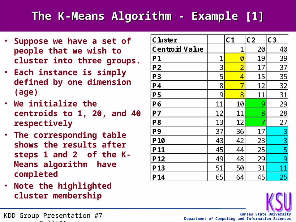
The K-Means Algorithm - Example [1]The K-Means Algorithm - Example [1]

• Suppose we have a set of people that we wish to cluster into three groups.

• Each instance is simply defined by one dimension (age)

• We initialize the centroids to 1, 20, and 40 respectively

• The corresponding table shows the results after steps 1 and 2 of the K-Means algorithm have completed

• Note the highlighted cluster membership

Cluster C1 C2 C3Centroid Value 1 20 40P1 1 0 19 39P2 3 2 17 37P3 5 4 15 35P4 8 7 12 32P5 9 8 11 31P6 11 10 9 29P7 12 11 8 28P8 13 12 7 27P9 37 36 17 3P10 43 42 23 3P11 45 44 25 5P12 49 48 29 9P13 51 50 31 11P14 65 64 45 25




• After the steps 1 and 2 are complete we recalculate the centroid values which are now 5, 12, and 48 respectively.

• We then recalculate the distance metric for each instance (repeat step 2)

• P5 is now closer to C2 than to C1 therefore we must recalculate the means for centroids C1 and C2

• C3 did not have a change to its membership so we don’t have to recalculate it





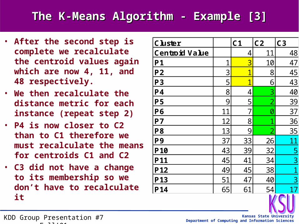
• After the second step is complete we recalculate the centroid values again which are now 4, 11, and 48 respectively.

• We then recalculate the distance metric for each instance (repeat step 2)

• P4 is now closer to C2 than to C1 therefore we must recalculate the means for centroids C1 and C2

• C3 did not have a change to its membership so we don’t have to recalculate it





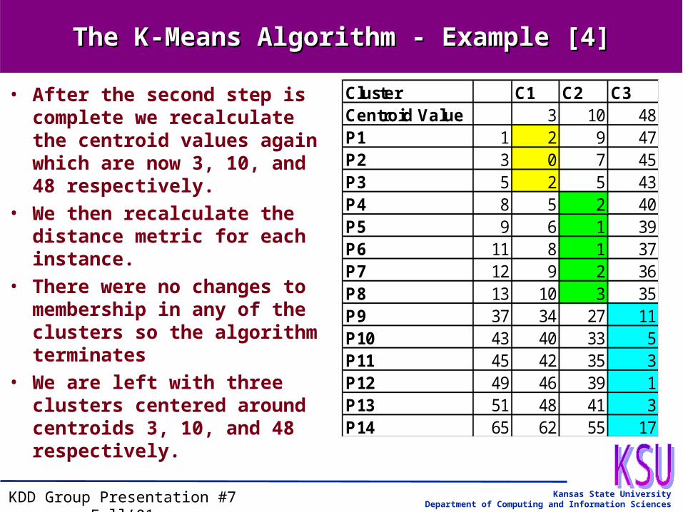
• After the second step is complete we recalculate the centroid values again which are now 3, 10, and 48 respectively.

• We then recalculate the distance metric for each instance.

• There were no changes to membership in any of the clusters so the algorithm terminates

• We are left with three clusters centered around centroids 3, 10, and 48 respectively.




Similarity, Association, and DistanceSimilarity, Association, and Distance

• Similarity, Association, and Distance– How do we convert our intuitive notions that members of a cluster have

some type of natural association to a representative metric?

– We could use a geometric conversion but there are problems with this� Many variable types, such as categorical variables and many numerical variables

such as rankings, cannot be converted.� In a database the contributions of one dimension may be more important than

another

– To understand these issues we must review measurement theory [3] � nominal - has no meaning; e.g. sports uniform numbers� ordinal - means one before other; e.g. class rank� interval - distance between two observations; no well understood zero; Temp.� ratio - has well understood zero; e.g. feet to meters� absolute - no conversion required; eg. lines of code

– Two of the most often used measures include� Euclidian distance - the square root of the sum of the squared distances� Number of common features - count of the degree of overlap which could

produce a ratio of number of matches to total number of fields



K, Weights, and ScalingK, Weights, and Scaling

• How do we choose K?– In many cases we have no prior knowledge of the number of clusters there should be– K is often chosen at random and with the results tested for the cluster strength; eg.

average distance between records in a cluster– Subjective evaluation is also required– K could be a hyper-parameter with fitness determined by a cluster strength metric

• Weighting and Scaling of variables (A Data Cleansing Process)– Scaling deals with the problem that different variables are measured in different units

� Converting all measurements to scale; eg. Feet, inches, and miles to inches� How about different types of measurements? This is a problem!� We can overcome this somewhat by mapping all variables to a common range so that a

change in ratio is comparable between the variables

– Weighting deals with the problem that we care about some variables more than others� Weighting can be used to bias one field over another� It can also be used as an optimization parameter with GA’s



Agglomerative AlgorithmsAgglomerative Algorithms

• Agglomerative Methods– Start out with each data point forming its own cluster and gradually merge

clusters until all points have gathered together to form one big cluster

– Preserves history of the cluster evolution

– Considered hierarchical

– The cluster distance metric used for merging can be one of the following:� Single Linkage: Distance between the closest members of each cluster� Complete Linkage: Distance between most distant members of each cluster� Comparison of centroids: Distance between the centroids of each cluster



Agglomeration by Single LinkageAgglomeration by Single Linkage

• Clustering People by Age– Use single linkage on a one dimensional vector

– Create clusters based on an age difference of one years

Dist43210 1 3 5 8 9 11 12 13 37 43 45 49 51 65

Clusters

Age In Years



Agglomeration By Comparison of CentroidsAgglomeration By Comparison of Centroids

• Minimal Spanning Tree Clustering (MSTC)

– Step 1 - Initialize the set of clusters

� The set of clusters is set to be the set of points. (i.e. - each point is a cluster)

– Step 2 - Calculate the cluster center

� The distance between each cluster center is calculated with respect to all other cluster centers.

� The two clusters with the minimum distance between them are fused to form a single cluster.

– Step 3 - Repeat

� Repeat Step 2 until all components are grouped into the final required set of clusters.



MSTC - ExampleMSTC - Example

• Mess personnel would like to identify four groups of food items from a larger group of seven food items so that if the soldiers select at least one item from each of the group they will obtain a certain fat and protein content.

• The seven food items will be grouped into four groups of food items based on the abundance of fat and protein content in the food.

• The following is the table that gives the fat and protein content in the food items.

Food item # Protein content, P Fat content, FFood item #1 1.1 60Food item #2 8.2 20Food item #3 4.2 35Food item #4 1.5 21Food item #5 7.6 15Food item #6 2 55Food item #7 3.9 39



MSTC - Example - Step 1MSTC - Example - Step 1

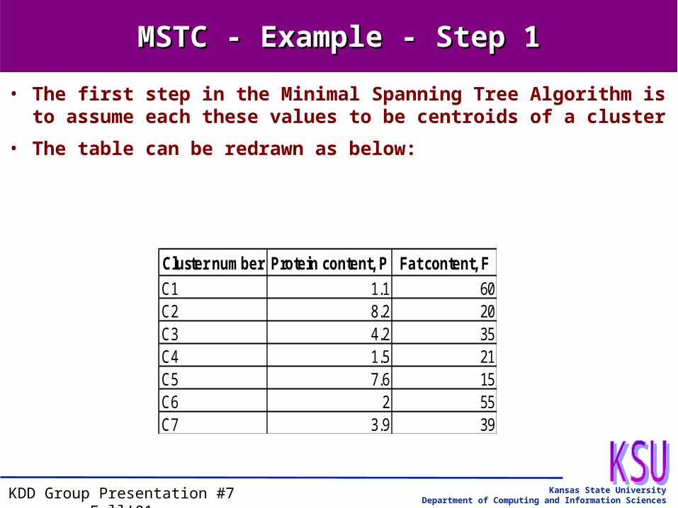
• The first step in the Minimal Spanning Tree Algorithm is to assume each these values to be centroids of a cluster

• The table can be redrawn as below:

Cluster number Protein content, P Fat content, F

C1 1.1 60C2 8.2 20C3 4.2 35C4 1.5 21C5 7.6 15C6 2 55C7 3.9 39



MSTC - Example - Step 2 [1]MSTC - Example - Step 2 [1]

• Step 2: Calculate the distance between every two of the centroids using the Euclidean metric.

• For example, the distance between C1 and C2 is calculated.




• The results are formulated into a table as shown below:

Cluster C1 C2 C3 C4 C5 C6 C7C1 0 40.62 25.19 39 45.46 5.08 21.18C2 known 0 15.52 6.77 5.03 35.54 19.48C3 known known 0 14.25 20.28 20.12 4.01C4 known known known 0 8.55 34 18.19C5 known known known known 0 40.39 24.28C6 known known known known known 0 16.11C7 known known known known known known 0




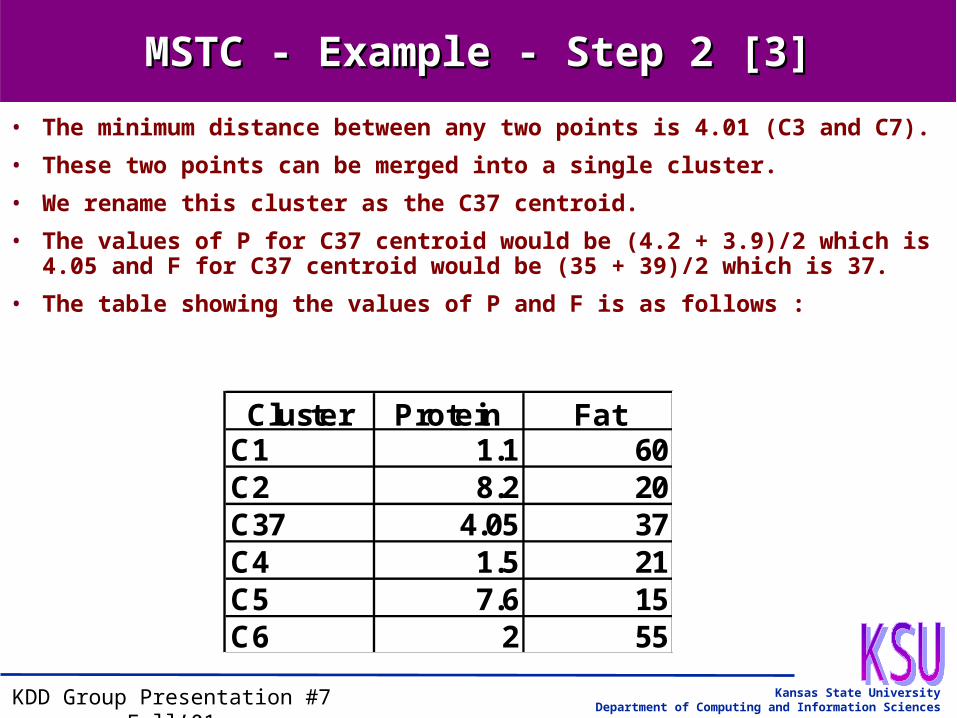
• The minimum distance between any two points is 4.01 (C3 and C7).

• These two points can be merged into a single cluster.

• We rename this cluster as the C37 centroid.

• The values of P for C37 centroid would be (4.2 + 3.9)/2 which is 4.05 and F for C37 centroid would be (35 + 39)/2 which is 37.

• The table showing the values of P and F is as follows :

Cluster Protein Fat C1 1.1 60C2 8.2 20C37 4.05 37C4 1.5 21C5 7.6 15C6 2 55




• The third step is to repeat the second step until the number of clusters is reduced to 4.

• This step means that the distance between any of the two points taken together is to be calculated as described above.

• The recalculated distances are given below :

Cluster C1 C2 C37 C4 C5 C6C1 0 40.62 23.18 39 45.46 5.08C2 known 0 17.49 6.77 5.03 35.54C37 known known 0 16.2 22.28 18.11C4 known known known 0 8.55 34C5 known known known known 0 40.26C6 known known known known known 0




• The minimum distance between any two points is 5.03 and this distance is between C2 and C5.

• These two points can be merged into a single point and is called the C25 centroid.

• The values of P for C25 centroid would be (8.2 + 7.6)/2 which is 7.90 and F for C25 centroid would be (15 + 20)/2 which is 17.5.


Cluster Protein Fat C1 1.1 60C25 7.9 17.5C37 4.05 37C4 1.5 21C6 2 55




• Next, we need to find the distance between each of the two points taken together as in step 2.

• The distances are calculated and displayed in the table given below :

Cluster C1 C25 C37 C4 C6C1 0 43.04 23.18 39 5.08C25 known 0 19.87 7.29 37.96C37 known known 0 16.2 18.11C4 known known known 0 34C6 known known known known 0




• The minimum distance between any two points is 5.08. This distance is between C1 and C6.

• These two points can be merged into a single point and is called the C16 centroid.

• The value of P for C16 centroid are be (1.1 + 2.0)/2 which is 1.55 and F for C16 centroid is (55 + 60)/2 which is 57.50.

• Finally, the data is divided into four groups of food items (clusters) with the fat and protein contents as specified (four centroids).


Cluster Protein Fat C16 1.55 57.5C25 7.9 17.5C37 4.05 37C4 1.5 21



Two-level ApproachTwo-level Approach

• Self-Organizing Map (SOM) [4]– Two-level approach to clustering

– Step 1: From N samples we create M prototypes� Each prototype is a two-dimensional grid of map units

– Step 2: From the M prototypes we apply a conventional method of clustering such as an agglomerative method or a variation of K-Means

– One of the benefits behind a two-level approach is that we can significantly reduce the computational cost



Summary and DiscussionSummary and Discussion

• Clustering is a data mining activity which allows us to make sense out of the data

• Unsupervised Learning

• We looked at two types of algorithms– Nonheirarchical; e.g. K-Means– Herirachical; e.g. Agglomeration Algorithms such as MSTC

• We discussed issues, parameters, and optimizations which can be done – Similarity, Association, and Distance– Choosing K, Scaling, and weighting– Use of Genetic Algorithms for optimization of the hyper-parameters

• Finally we discussed a hybrid approach – Self-Organizing Maps – Use two-levels in the clustering process

• The next step will be to look at specific algorithms and compare them to K-Means (the benchmark)

• Much room for research in this field



BibliographyBibliography

• [1] Menasce’, D.A., Denning, P.J., et.al., DAU Stat Refresher Module, http://cne.gmu.edu/modules/dau/stat/clustgalgs/clust4_frm.html, Center for the New Engineer, George Mason University, Fairfax, Virginia

• [2] Berry, M. J. A., and Linoff, G. S. Data Mining Techniques for Marketing, Sales, and Customer Support. John Wiley and Sons, New York, NY, 1997.

• [3] Gustafson, D., CIS 740 Software Engineering Course Notes, Fall, 2000

• [4] Vesanto, J. and Alhoniemi, E., Clustering of the Self-Organizing Map, IEEE Transactions on Neural Networks, accepted

Kansas State University Department of Computing and Information Sciences KDD Group Presentation #7...

Documents

Transcript of Kansas State University Department of Computing and Information Sciences KDD Group Presentation #7...