Kansas State University Department of Computing and Information Sciences CIS 732: Machine Learning...

Kansas State University

Department of Computing and Information SciencesCIS 732: Machine Learning and Pattern Recognition

Friday, 01 February 2008

William H. Hsu

Department of Computing and Information Sciences, KSUhttp://www.cis.ksu.edu/~bhsu

Readings:

Chapter 3.6-3.8, Mitchell

Decision Trees,Occam’s Razor, and Overfitting

Lecture 5 of 42Lecture 5 of 42



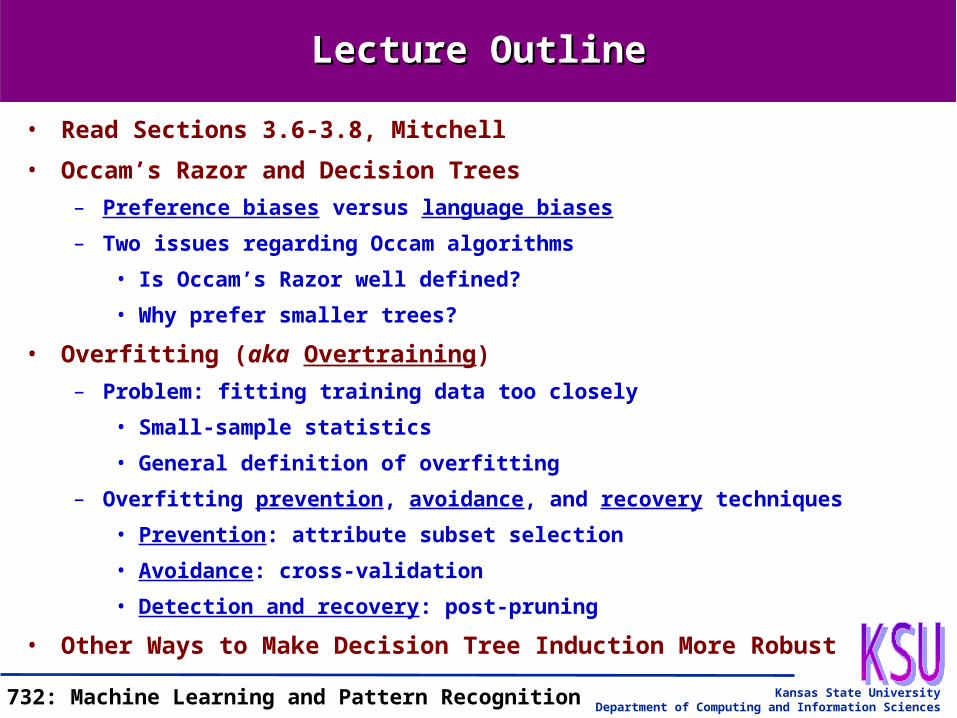
Lecture OutlineLecture Outline

• Read Sections 3.6-3.8, Mitchell

• Occam’s Razor and Decision Trees

– Preference biases versus language biases

– Two issues regarding Occam algorithms

• Is Occam’s Razor well defined?

• Why prefer smaller trees?

• Overfitting (aka Overtraining)

– Problem: fitting training data too closely

• Small-sample statistics

• General definition of overfitting

– Overfitting prevention, avoidance, and recovery techniques

• Prevention: attribute subset selection

• Avoidance: cross-validation

• Detection and recovery: post-pruning

• Other Ways to Make Decision Tree Induction More Robust



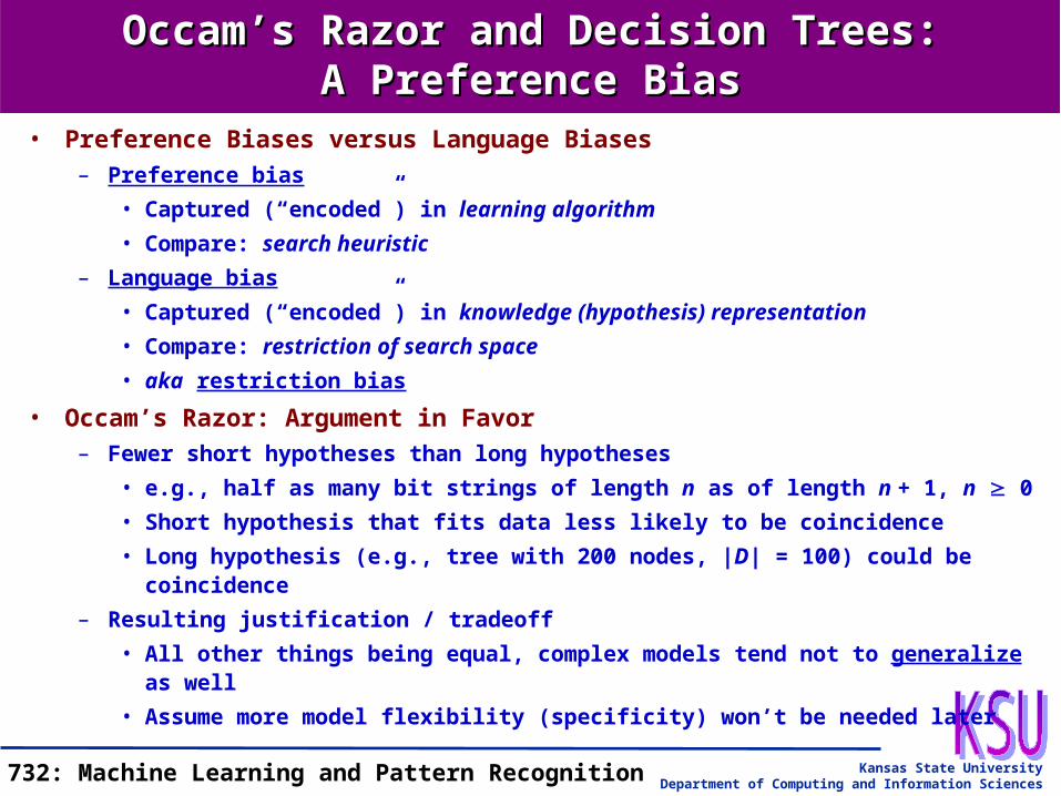
Occam’s Razor and Decision Trees:Occam’s Razor and Decision Trees:A Preference BiasA Preference Bias

• Preference Biases versus Language Biases– Preference bias

• Captured (“encoded”) in learning algorithm

• Compare: search heuristic

– Language bias

• Captured (“encoded”) in knowledge (hypothesis) representation

• Compare: restriction of search space

• aka restriction bias

• Occam’s Razor: Argument in Favor– Fewer short hypotheses than long hypotheses

• e.g., half as many bit strings of length n as of length n + 1, n 0

• Short hypothesis that fits data less likely to be coincidence

• Long hypothesis (e.g., tree with 200 nodes, |D| = 100) could be coincidence

– Resulting justification / tradeoff

• All other things being equal, complex models tend not to generalize as well

• Assume more model flexibility (specificity) won’t be needed later



Occam’s Razor and Decision Trees:Occam’s Razor and Decision Trees:Two IssuesTwo Issues

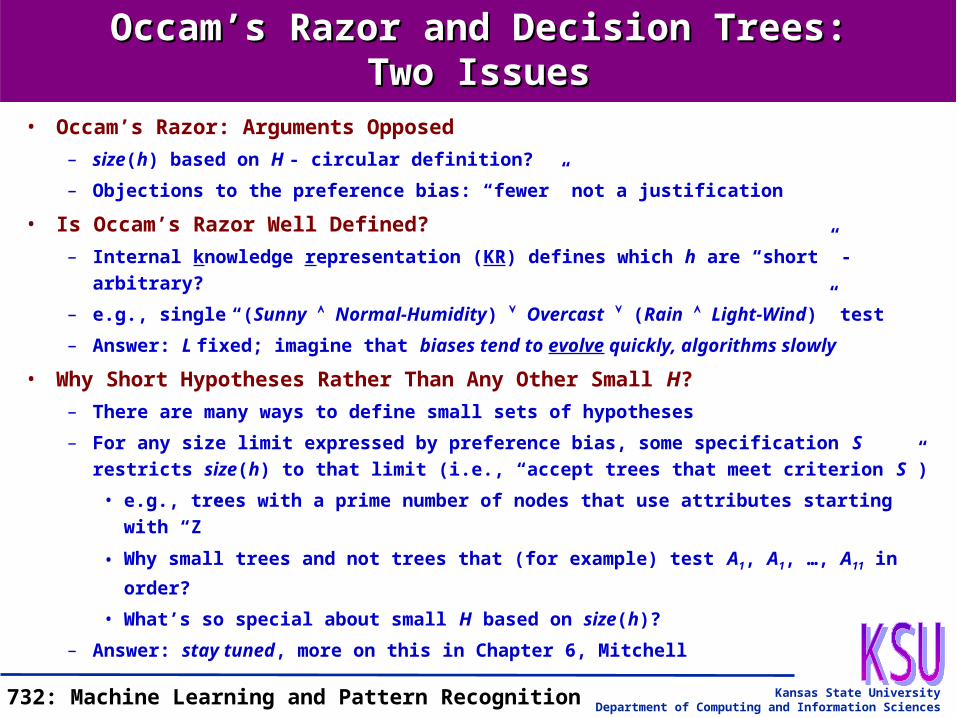
• Occam’s Razor: Arguments Opposed

– size(h) based on H - circular definition?

– Objections to the preference bias: “fewer” not a justification

• Is Occam’s Razor Well Defined?

– Internal knowledge representation (KR) defines which h are “short” - arbitrary?

– e.g., single “(Sunny Normal-Humidity) Overcast (Rain Light-Wind)” test

– Answer: L fixed; imagine that biases tend to evolve quickly, algorithms slowly

• Why Short Hypotheses Rather Than Any Other Small H?

– There are many ways to define small sets of hypotheses

– For any size limit expressed by preference bias, some specification S restricts

size(h) to that limit (i.e., “accept trees that meet criterion S”)

• e.g., trees with a prime number of nodes that use attributes starting with “Z”

• Why small trees and not trees that (for example) test A1, A1, …, A11 in order?

• What’s so special about small H based on size(h)?

– Answer: stay tuned, more on this in Chapter 6, Mitchell



Overfitting in Decision Trees:Overfitting in Decision Trees:An ExampleAn Example

• Recall: Induced Tree

• Noisy Training Example– Example 15: <Sunny, Hot, Normal, Strong, ->

• Example is noisy because the correct label is +

• Previously constructed tree misclassifies it

– How shall the DT be revised (incremental learning)?

– New hypothesis h’ = T’ is expected to perform worse than h = T

Outlook?

Wind?Yes

Sunny Overcast Rain

No

High Normal

YesNo

Strong Light

Boolean Decision Treefor Concept PlayTennis

Humidity?

1,2,3,4,5,6,7,8,9,10,11,12,13,14[9+,5-]

1,2,8,9,11[2+,3-]

3,7,12,13[4+,0-]

4,5,6,10,14[3+,2-]

1,2,8[0+,3-]

6,14[0+,2-]

4,5,10[3+,0-]

Temp?

Hot CoolMild

9,11,15[2+,1-]

15[0+,1-]

No Yes

11[1+,0-]

9[1+,0-]

YesMay fit noise or

other coincidental regularities



Overfitting in Inductive LearningOverfitting in Inductive Learning

• Definition– Hypothesis h overfits training data set D if an alternative hypothesis h’ such

that errorD(h) < errorD(h’) but errortest(h) > errortest(h’)

– Causes: sample too small (decisions based on too little data); noise; coincidence

• How Can We Combat Overfitting?– Analogy with computer virus infection, process deadlock

– Prevention

• Addressing the problem “before it happens”

• Select attributes that are relevant (i.e., will be useful in the model)

• Caveat: chicken-egg problem; requires some predictive measure of relevance

– Avoidance

• Sidestepping the problem just when it is about to happen

• Holding out a test set, stopping when h starts to do worse on it

– Detection and Recovery

• Letting the problem happen, detecting when it does, recovering afterward

• Build model, remove (prune) elements that contribute to overfitting



• How Can We Combat Overfitting?– Prevention (more on this later)

• Select attributes that are relevant (i.e., will be useful in the DT)

• Predictive measure of relevance: attribute filter or subset selection wrapper

– Avoidance

• Holding out a validation set, stopping when h T starts to do worse on it

• How to Select “Best” Model (Tree)– Measure performance over training data and separate validation set

– Minimum Description Length (MDL): minimize size(h T) + size (misclassifications (h T))

Decision Tree Learning:Decision Tree Learning:Overfitting Prevention and AvoidanceOverfitting Prevention and Avoidance

Size of tree (number of nodes)

0 10 20 30 40 50 60 70 80 90 100

Ac

cu

rac

y

0.90.850.8

0.750.7

0.650.6

0.550.5

On training data

On test data



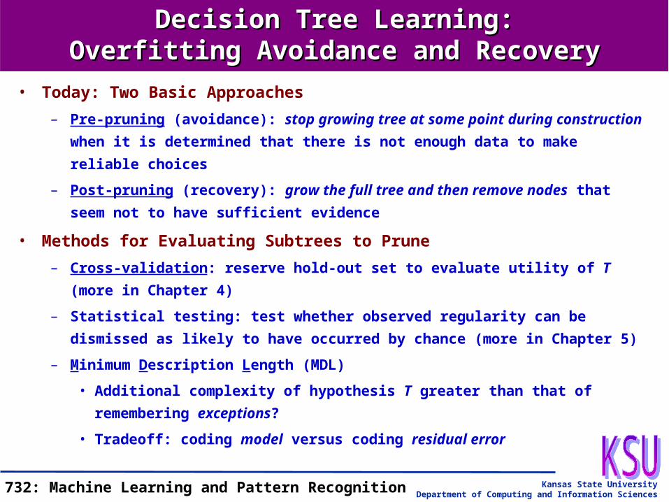
Decision Tree Learning:Decision Tree Learning:Overfitting Avoidance and RecoveryOverfitting Avoidance and Recovery

• Today: Two Basic Approaches

– Pre-pruning (avoidance): stop growing tree at some point during construction

when it is determined that there is not enough data to make reliable choices

– Post-pruning (recovery): grow the full tree and then remove nodes that seem not

to have sufficient evidence

• Methods for Evaluating Subtrees to Prune

– Cross-validation: reserve hold-out set to evaluate utility of T (more in Chapter 4)

– Statistical testing: test whether observed regularity can be dismissed as likely to

have occurred by chance (more in Chapter 5)

– Minimum Description Length (MDL)

• Additional complexity of hypothesis T greater than that of remembering

exceptions?

• Tradeoff: coding model versus coding residual error



Reduced-Error PruningReduced-Error Pruning

• Post-Pruning, Cross-Validation Approach

• Split Data into Training and Validation Sets

• Function Prune(T, node)

– Remove the subtree rooted at node

– Make node a leaf (with majority label of associated examples)

• Algorithm Reduced-Error-Pruning (D)

– Partition D into Dtrain (training / “growing”), Dvalidation (validation / “pruning”)

– Build complete tree T using ID3 on Dtrain

– UNTIL accuracy on Dvalidation decreases DO

FOR each non-leaf node candidate in T

Temp[candidate] Prune (T, candidate)

Accuracy[candidate] Test (Temp[candidate], Dvalidation)

T T’ Temp with best value of Accuracy (best increase; greedy)

– RETURN (pruned) T



Effect of Reduced-Error PruningEffect of Reduced-Error Pruning

Size of tree (number of nodes)

0 10 20 30 40 50 60 70 80 90 100

Ac

cu

rac

y

0.90.850.8

0.750.7

0.650.6

0.550.5

On training data

On test data

Post-pruned treeon test data

• Reduction of Test Error by Reduced-Error Pruning

– Test error reduction achieved by pruning nodes

– NB: here, Dvalidation is different from both Dtrain and Dtest

• Pros and Cons

– Pro: Produces smallest version of most accurate T’ (subtree of T)

– Con: Uses less data to construct T

• Can afford to hold out Dvalidation?

• If not (data is too limited), may make error worse (insufficient Dtrain)



Rule Post-PruningRule Post-Pruning

• Frequently Used Method

– Popular anti-overfitting method; perhaps most popular pruning method

– Variant used in C4.5, an outgrowth of ID3

• Algorithm Rule-Post-Pruning (D)

– Infer T from D (using ID3) - grow until D is fit as well as possible (allow overfitting)

– Convert T into equivalent set of rules (one for each root-to-leaf path)

– Prune (generalize) each rule independently by deleting any preconditions whose

deletion improves its estimated accuracy

– Sort the pruned rules

• Sort by their estimated accuracy

• Apply them in sequence on Dtest



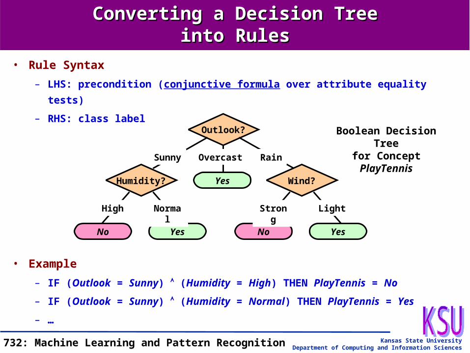
Converting a Decision TreeConverting a Decision Treeinto Rulesinto Rules

• Rule Syntax

– LHS: precondition (conjunctive formula over attribute equality tests)

– RHS: class label

• Example

– IF (Outlook = Sunny) (Humidity = High) THEN PlayTennis = No

– IF (Outlook = Sunny) (Humidity = Normal) THEN PlayTennis = Yes

– …

Yes

Overcast

Outlook?

Humidity?

Sunny

No

High

Yes

Normal

Wind?

Rain

No

Strong

Yes

Light

Boolean Decision Treefor Concept PlayTennis



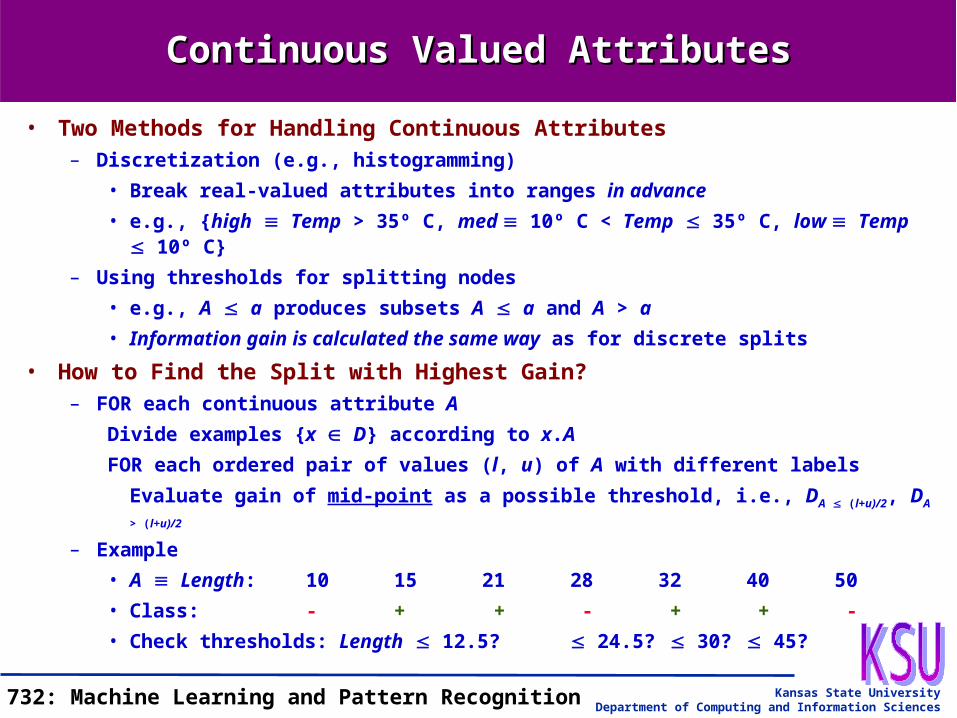
Continuous Valued AttributesContinuous Valued Attributes

• Two Methods for Handling Continuous Attributes– Discretization (e.g., histogramming)

• Break real-valued attributes into ranges in advance

• e.g., {high Temp > 35º C, med 10º C < Temp 35º C, low Temp 10º C}

– Using thresholds for splitting nodes

• e.g., A a produces subsets A a and A > a

• Information gain is calculated the same way as for discrete splits

• How to Find the Split with Highest Gain?– FOR each continuous attribute A

Divide examples {x D} according to x.A

FOR each ordered pair of values (l, u) of A with different labels

Evaluate gain of mid-point as a possible threshold, i.e., DA (l+u)/2, DA > (l+u)/2

– Example

• A Length: 10 15 21 28 32 40 50

• Class: - + + - + + -

• Check thresholds: Length 12.5? 24.5? 30? 45?



Attributes with Many ValuesAttributes with Many Values

• Problem– If attribute has many values, Gain(•) will select it (why?)

– Imagine using Date = 06/03/1996 as an attribute!

• One Approach: Use GainRatio instead of Gain

– SplitInformation: directly proportional to c = | values(A) |

– i.e., penalizes attributes with more values

• e.g., suppose c1 = cDate = n and c2 = 2

• SplitInformation (A1) = lg(n), SplitInformation (A2) = 1

• If Gain(D, A1) = Gain(D, A2), GainRatio (D, A1) << GainRatio (D, A2)

– Thus, preference bias (for lower branch factor) expressed via GainRatio(•)

values(A)v

vv

values(A)vv

v

D

D

D

DAD,mationSplitInfor

AD,mationSplitInfor

AD,GainAD,GainRatio

DHD

DDH-AD,Gain

lg



Attributes with CostsAttributes with Costs

• Application Domains– Medical: Temperature has cost $10; BloodTestResult, $150; Biopsy, $300

• Also need to take into account invasiveness of the procedure (patient utility)

• Risk to patient (e.g., amniocentesis)

– Other units of cost

• Sampling time: e.g., robot sonar (range finding, etc.)

• Risk to artifacts, organisms (about which information is being gathered)

• Related domains (e.g., tomography): nondestructive evaluation

• How to Learn A Consistent Tree with Low Expected Cost?– One approach: replace gain by Cost-Normalized-Gain

– Examples of normalization functions

• [Nunez, 1988]:

• [Tan and Schlimmer, 1990]:

where w determines importance of cost

AD,Cost

AD,GainAD,Gain-Normalized-Cost

2

0,1w

AD,CostAD,Gain-Normalized-Cost

w

AD,Gain

1

1-2



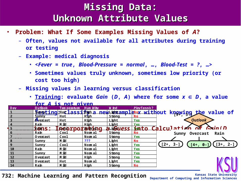
Missing Data:Missing Data:Unknown Attribute ValuesUnknown Attribute Values

• Problem: What If Some Examples Missing Values of A?– Often, values not available for all attributes during training or testing

– Example: medical diagnosis

• <Fever = true, Blood-Pressure = normal, …, Blood-Test = ?, …>

• Sometimes values truly unknown, sometimes low priority (or cost too high)

– Missing values in learning versus classification

• Training: evaluate Gain (D, A) where for some x D, a value for A is not given

• Testing: classify a new example x without knowing the value of A

• Solutions: Incorporating a Guess into Calculation of Gain(D, A)

Outlook

[9+, 5-]

[3+, 2-]

Rain

[2+, 3-]

Sunny Overcast

[4+, 0-]

Day Outlook Temperature Humidity Wind PlayTennis?1 Sunny Hot High Light No2 Sunny Hot High Strong No3 Overcast Hot High Light Yes4 Rain Mild High Light Yes5 Rain Cool Normal Light Yes6 Rain Cool Normal Strong No7 Overcast Cool Normal Strong Yes8 Sunny Mild ??? Light No9 Sunny Cool Normal Light Yes10 Rain Mild Normal Light Yes11 Sunny Mild Normal Strong Yes12 Overcast Mild High Strong Yes13 Overcast Hot Normal Light Yes14 Rain Mild High Strong No



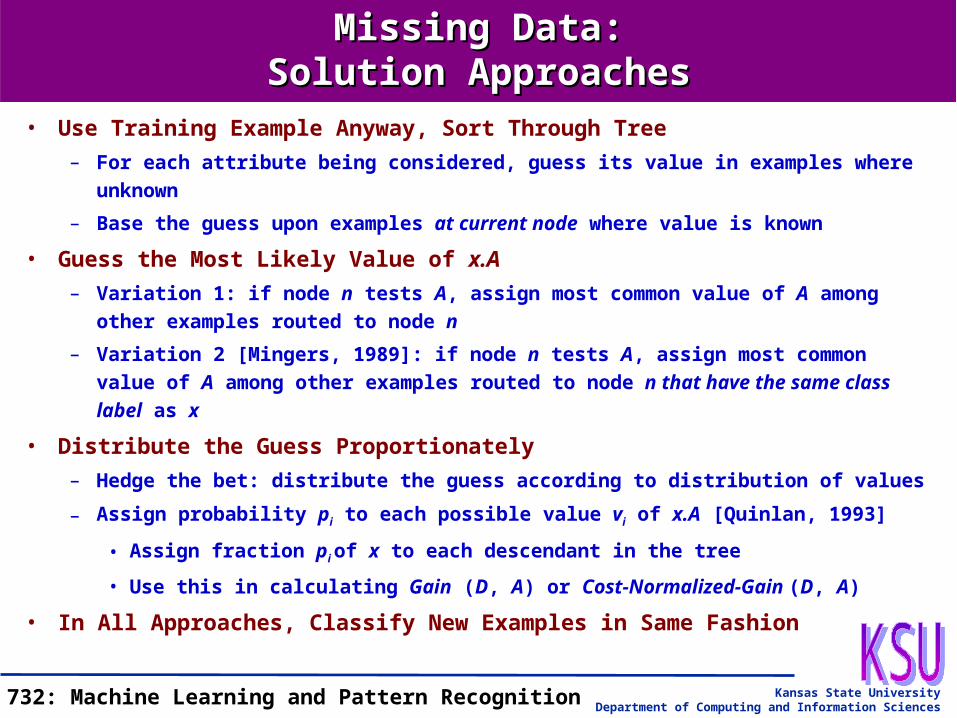
Missing Data:Missing Data:Solution ApproachesSolution Approaches

• Use Training Example Anyway, Sort Through Tree

– For each attribute being considered, guess its value in examples where unknown

– Base the guess upon examples at current node where value is known

• Guess the Most Likely Value of x.A

– Variation 1: if node n tests A, assign most common value of A among other

examples routed to node n

– Variation 2 [Mingers, 1989]: if node n tests A, assign most common value of A

among other examples routed to node n that have the same class label as x

• Distribute the Guess Proportionately

– Hedge the bet: distribute the guess according to distribution of values

– Assign probability pi to each possible value vi of x.A [Quinlan, 1993]

• Assign fraction pi of x to each descendant in the tree

• Use this in calculating Gain (D, A) or Cost-Normalized-Gain (D, A)

• In All Approaches, Classify New Examples in Same Fashion



Missing Data:Missing Data:An ExampleAn Example

• Guess the Most Likely Value of x.A

– Variation 1: Humidity = High or Normal (High: Gain = 0.97, Normal: < 0.97)

– Variation 2: Humidity = High (all No cases are High)

• Probabilistically Weighted Guess

– Guess 0.5 High, 0.5 Normal

– Gain < 0.97

• Test Case: <?, Hot, Normal, Strong>

– 1/3 Yes + 1/3 Yes + 1/3 No = Yes

Day Outlook Temperature Humidity Wind PlayTennis?1 Sunny Hot High Light No2 Sunny Hot High Strong No3 Overcast Hot High Light Yes4 Rain Mild High Light Yes5 Rain Cool Normal Light Yes6 Rain Cool Normal Strong No7 Overcast Cool Normal Strong Yes8 Sunny Mild ??? Light No9 Sunny Cool Normal Light Yes10 Rain Mild Normal Light Yes11 Sunny Mild Normal Strong Yes12 Overcast Mild High Strong Yes13 Overcast Hot Normal Light Yes14 Rain Mild High Strong No

Humidity? Wind?Yes

YesNo YesNo

Outlook?

1,2,3,4,5,6,7,8,9,10,11,12,13,14[9+,5-]

Sunny Overcast Rain

1,2,8,9,11[2+,3-]

3,7,12,13[4+,0-]

4,5,6,10,14[3+,2-]

High Normal

1,2,8[0+,3-]

9,11[2+,0-]

Strong Light

6,14[0+,2-]

4,5,10[3+,0-]



Replication in Decision TreesReplication in Decision Trees

• Decision Trees: A Representational Disadvantage

– DTs are more complex than some other representations

– Case in point: replications of attributes

• Replication Example

– e.g., Disjunctive Normal Form (DNF): (a b) (c d e)

– Disjuncts must be repeated as subtrees

• Partial Solution Approach

– Creation of new features

– aka constructive induction (CI)

– More on CI in Chapter 10, Mitchell

a?

b?c?

c?

d?

e?

d?

e?

+-

+

+

-

-

-

-

-

0 1

0 1

0 1

0 1 0 1

0 1

0

0 1



FringeFringe::Constructive Induction in Decision TreesConstructive Induction in Decision Trees

• Synthesizing New Attributes

– Synthesize (create) a new attribute from the conjunction of the last two attributes

before a + node

– aka feature construction

• Example

– (a b) (c d e)

– A = d e

– B = a b

• Repeated application

– C = A c

– Correctness?

– Computation?

a?

b?c?

c?

d?

e?

d?

e?

+-

+

+

-

-

-

-

-

0 1

0 1

0 1

0 1 0 1

0 1

0

0 1

B?

c?

A?-

+

0 1

0 1

0 1-

+

B?

C?

- +

0 1

0 1+



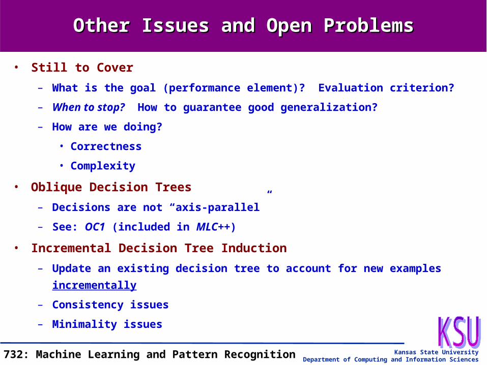
Other Issues and Open ProblemsOther Issues and Open Problems

• Still to Cover

– What is the goal (performance element)? Evaluation criterion?

– When to stop? How to guarantee good generalization?

– How are we doing?

• Correctness

• Complexity

• Oblique Decision Trees

– Decisions are not “axis-parallel”

– See: OC1 (included in MLC++)

• Incremental Decision Tree Induction

– Update an existing decision tree to account for new examples incrementally

– Consistency issues

– Minimality issues



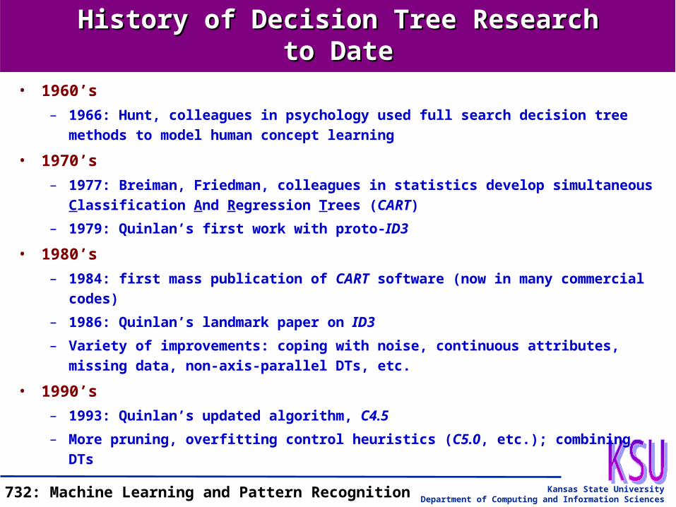
History of Decision Tree ResearchHistory of Decision Tree Researchto Dateto Date

• 1960’s

– 1966: Hunt, colleagues in psychology used full search decision tree methods to

model human concept learning

• 1970’s

– 1977: Breiman, Friedman, colleagues in statistics develop simultaneous

Classification And Regression Trees (CART)

– 1979: Quinlan’s first work with proto-ID3

• 1980’s

– 1984: first mass publication of CART software (now in many commercial codes)

– 1986: Quinlan’s landmark paper on ID3

– Variety of improvements: coping with noise, continuous attributes, missing data,

non-axis-parallel DTs, etc.

• 1990’s

– 1993: Quinlan’s updated algorithm, C4.5

– More pruning, overfitting control heuristics (C5.0, etc.); combining DTs



TerminologyTerminology

• Occam’s Razor and Decision Trees– Preference biases: captured by hypothesis space search algorithm

– Language biases : captured by hypothesis language (search space definition)

• Overfitting– Overfitting: h does better than h’ on training data and worse on test data

– Prevention, avoidance, and recovery techniques

• Prevention: attribute subset selection

• Avoidance: stopping (termination) criteria, cross-validation, pre-pruning

• Detection and recovery: post-pruning (reduced-error, rule)

• Other Ways to Make Decision Tree Induction More Robust– Inequality DTs (decision surfaces): a way to deal with continuous attributes

– Information gain ratio: a way to normalize against many-valued attributes

– Cost-normalized gain: a way to account for attribute costs (utilities)

– Missing data: unknown attribute values or values not yet collected

– Feature construction: form of constructive induction; produces new attributes

– Replication: repeated attributes in DTs



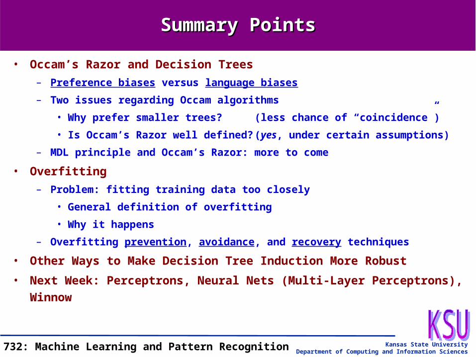
Summary PointsSummary Points

• Occam’s Razor and Decision Trees

– Preference biases versus language biases

– Two issues regarding Occam algorithms

• Why prefer smaller trees? (less chance of “coincidence”)

• Is Occam’s Razor well defined? (yes, under certain assumptions)

– MDL principle and Occam’s Razor: more to come

• Overfitting

– Problem: fitting training data too closely

• General definition of overfitting

• Why it happens

– Overfitting prevention, avoidance, and recovery techniques

• Other Ways to Make Decision Tree Induction More Robust

• Next Week: Perceptrons, Neural Nets (Multi-Layer Perceptrons), Winnow

Kansas State University Department of Computing and Information Sciences CIS 732: Machine Learning...

Documents

Transcript of Kansas State University Department of Computing and Information Sciences CIS 732: Machine Learning...