Report No. K-TRAN: KSU-14-4 ▪ FINAL REPORT▪ September 2015

Kansas Department of Transportation Column Expert: Ultimate Shear Capacity of Circular Columns Using the Simplified Modified Compression Field Theory

AlaaEldin Abouelleil, M.S.Hayder Rasheed, Ph.D., P.E., FASCE

Kansas State University Transportation Center

i

Form DOT F 1700.7 (8-72)

1 Report No. K-TRAN: KSU-14-4

2 Government Accession No.

3 Recipient Catalog No.

4 Title and Subtitle Kansas Department of Transportation Column Expert: Ultimate Shear Capacity of Circular Columns Using the Simplified Modified Compression Field Theory

5 Report Date September 2015

6 Performing Organization Code

7 Author(s) AlaaEldin Abouelleil, M.S., and Hayder Rasheed, Ph.D., P.E., FASCE

7 Performing Organization Report No.

9 Performing Organization Name and Address Kansas State University Transportation Center Department of Civil Engineering 2126 Fiedler Hall Manhattan, Kansas 66506

10 Work Unit No. (TRAIS)

11 Contract or Grant No. C1972

12 Sponsoring Agency Name and Address Kansas Department of Transportation Bureau of Research 2300 SW Van Buren Topeka, Kansas 66611-1195

13 Type of Report and Period Covered Final Report July 2013–June 2015

14 Sponsoring Agency Code RE-0625-01

15 Supplementary Notes For more information write to address in block 9.

The importance of the analysis of circular columns to accurately predict their ultimate confined capacity under shear-flexure-axial force interaction domain is recognized in light of the extreme load event imposed by the current American Association of State Highway and Transportation Officials (AASHTO) Load and Resistance Factor Design (LRFD) Bridge Construction Specifications (AASHTO, 2014). In this study, various procedures for computing shear strength are reviewed. Then, the current procedure adopted by AASHTO LRFD specifications, based on the Simplified Modified Compression Field Theory, is evaluated for non-prestressed circular concrete bridge piers. This evaluation is benchmarked against experimental data available in the literature, and against Response 2000 freeware program that depicts interaction diagrams based on AASHTO (1999) LRFD requirements. Differences in results are discussed and future improvements are proposed. A new approach is presented to improve the accuracy of AASHTO LRFD calculations. The main parameters that control the cross section shear strength are discussed based on the experimental results and comparisons. 17 Key Words

Shear Capacity, Circular Columns, Concrete Shear Resistance

18 Distribution Statement No restrictions. This document is available to the public through the National Technical Information Service www.ntis.gov.

19 Security Classification (of this report)

Unclassified

20 Security Classification (of this page) Unclassified

21 No. of pages 129

22 Price

ii

This page intentionally left blank.

iii

Kansas Department of Transportation Column Expert: Ultimate Shear Capacity of Circular Columns Using the

Simplified Modified Compression Field Theory

Final Report

Prepared by

AlaaEldin Abouelleil, M.S. Hayder Rasheed, Ph.D., P.E., FASCE

Kansas State University Transportation Center

A Report on Research Sponsored by

KANSAS DEPARTMENT OF TRANSPORTATION TOPEKA, KANSAS

and

KANSAS STATE UNIVERSITY TRANSPORTATION CENTER

MANHATTAN, KANSAS

September 2015

© Copyright 2015, Kansas Department of Transportation

iv

PREFACE The Kansas Department of Transportation’s (KDOT) Kansas Transportation Research and New-Developments (K-TRAN) Research Program funded this research project. It is an ongoing, cooperative and comprehensive research program addressing transportation needs of the state of Kansas utilizing academic and research resources from KDOT, Kansas State University and the University of Kansas. Transportation professionals in KDOT and the universities jointly develop the projects included in the research program.

NOTICE The authors and the state of Kansas do not endorse products or manufacturers. Trade and manufacturers names appear herein solely because they are considered essential to the object of this report. This information is available in alternative accessible formats. To obtain an alternative format, contact the Office of Public Affairs, Kansas Department of Transportation, 700 SW Harrison, 2nd Floor – West Wing, Topeka, Kansas 66603-3745 or phone (785) 296-3585 (Voice) (TDD).

DISCLAIMER The contents of this report reflect the views of the authors who are responsible for the facts and accuracy of the data presented herein. The contents do not necessarily reflect the views or the policies of the state of Kansas. This report does not constitute a standard, specification or regulation.

v

Abstract

The importance of the analysis of circular columns to accurately predict their ultimate

confined capacity under shear-flexure-axial force interaction domain is recognized in light of the

extreme load event imposed by the current American Association of State Highway and

Transportation Officials (AASHTO) Load and Resistance Factor Design (LRFD) Bridge

Construction Specifications (AASHTO, 2014). In this study, various procedures for computing

shear strength are reviewed. Then, the current procedure adopted by AASHTO LRFD

specifications, based on the Simplified Modified Compression Field Theory, is evaluated for

non-prestressed circular concrete bridge piers. This evaluation is benchmarked against

experimental data available in the literature, and against Response 2000 freeware program that

depicts interaction diagrams based on AASHTO (1999) LRFD requirements. Differences in

results are discussed and future improvements are proposed. A new approach is presented to

improve the accuracy of AASHTO LRFD calculations. The main parameters that control the

cross section shear strength are discussed based on the experimental results and comparisons.

vi

Acknowledgements

This research was made possible by funding from the Kansas Department of

Transportation (KDOT) through its K-TRAN program. Special thanks are extended to John

Jones and Calvin Reed of KDOT, as well as Loren Risch, who has since retired from KDOT, for

their interest in this project and their continuous support and feedback that made it possible to

arrive at such important findings.

vii

Table of Contents

Abstract ........................................................................................................................................... v Acknowledgements ........................................................................................................................ vi Table of Contents .......................................................................................................................... vii List of Tables ................................................................................................................................. ix List of Figures ................................................................................................................................. x Chapter 1: Introduction ................................................................................................................... 1

1.1 Overview ............................................................................................................................... 1 1.2 Objectives ............................................................................................................................. 1 1.3 Scope ..................................................................................................................................... 1

Chapter 2: Literature Review .......................................................................................................... 3 2.1 Overview ............................................................................................................................... 3 2.2 Theoretical Treatments ......................................................................................................... 3

2.2.1 Approach of Priestley, Verma, and Xiao (1994) ........................................................... 3 2.2.2 Standards New Zealand (1995) ...................................................................................... 4 2.2.3 Applied Technology Council Report ATC-32 Shear Design Equations ....................... 5 2.2.4 California Department of Transportation Memo 20-4 (2010) ....................................... 5 2.2.5 Joint ASCE-ACI Task Committee 426 (1973) Shear Strength Approach ..................... 6 2.2.6 ACI Committee 318 (2011) ........................................................................................... 7 2.2.7 Modified Compression Field Theory ............................................................................. 7

2.3 Experimental Studies .......................................................................................................... 16 Chapter 3: Present Formulation .................................................................................................... 22

3.1 Overview ............................................................................................................................. 22 3.2 AASHTO (2014) LRFD Approach ..................................................................................... 22

3.2.1 Minimum Transverse Steel .......................................................................................... 22 3.2.2 Shear Resistance .......................................................................................................... 23 3.2.3 Determination of β and θ ............................................................................................. 24 3.2.4 Calculation of Longitudinal Axial Strain (εs) ............................................................. 25 3.2.5 Angle of Inclination of Transverse Reinforcement to Longitudinal Axis (α) Calculations ........................................................................................................................... 27 3.2.6 Effective Number of Legs of Transverse Steel in Shear Resistance Calculation ........ 28

Chapter 4: Implementation ........................................................................................................... 31 4.1 Overview ............................................................................................................................. 31 4.2 Input Parameters ................................................................................................................. 31 4.3 Effective Shear Area ........................................................................................................... 32

4.3.1 Effective Shear Depth Calculation (dv) ........................................................................ 32 4.4 Analysis Procedure ............................................................................................................. 33

4.4.1 Limits of Constraints .................................................................................................... 35 Chapter 5: Experimental Verification ........................................................................................... 38

5.1 Overview ............................................................................................................................. 38

viii

5.2 Database Criteria ................................................................................................................. 38 5.3 Comparisons Against Experimental Studies ....................................................................... 38 5.4 Comparisons against Response-2000 ................................................................................. 55 5.5 Database .............................................................................................................................. 62

Chapter 6: Software Development ................................................................................................ 75 6.1 Introduction ......................................................................................................................... 75 6.2 Input Interface ..................................................................................................................... 75 6.3 Output Interface .................................................................................................................. 77

Chapter 7: Complete Database Comparisons of AASHTO LRFD Approach .............................. 81 Chapter 8: Conclusions ............................................................................................................... 109 References ................................................................................................................................... 110

ix

List of Tables

Table 2.1: Ang et al. (1985) Columns Details and Results ........................................................... 19 Table 2.2: Ohtaki et al. (1996) Columns Details and Results ....................................................... 20 Table 2.3: Nelson (2000) Columns Details and Results ............................................................... 20 Table 2.4: Modified Compression Field Theory Experimental Program ..................................... 21 Table 5.1: Selected Sections ......................................................................................................... 39 Table 5.2: Selected Sections Properties ........................................................................................ 40 Table 5.3: Arakawa et al. (1987) Sections .................................................................................... 63 Table 5.4: Calderone, Lehman, and Moehle (2001) Sections ....................................................... 64 Table 5.5: Henry and Mahin (1999) Sections ............................................................................... 64 Table 5.6: Hamilton et al. (2002) Sections ................................................................................... 64 Table 5.7: Cheok and Stone (1986) Sections ................................................................................ 65 Table 5.8: Chai, Priestley, and Seible (1991) Sections ................................................................. 65 Table 5.9: Siryo (1975) Sections .................................................................................................. 65 Table 5.10: Kowalesky and Priestley (2000) Sections ................................................................. 66 Table 5.11: Hose, Seible, and Priestley (1997) Section and Elsanadedy (2002) Section ............. 66 Table 5.12: Moyer and Kowalsky (2003) Sections ...................................................................... 66 Table 5.13: Ng, Lam, and Kwan (2010) Sections ......................................................................... 67 Table 5.14: Kunnath et al. (1997) Sections................................................................................... 67 Table 5.15: Lehman and Moehle (2000) Sections ........................................................................ 68 Table 5.16: Lim and McLean (1991) Sections ............................................................................. 68 Table 5.17: Munro, Park, and Priestley (1976) Section and Iwasaki et al. (1986) Section .......... 68 Table 5.18: McDaniel (1997) Sections ......................................................................................... 69 Table 5.19: Jaradat (1996) Sections .............................................................................................. 69 Table 5.20: Nelson (2000) Sections .............................................................................................. 69 Table 5.21: Priestley et al. (1994) Sections .................................................................................. 70 Table 5.22: Petrovski and Ristic (1984) Sections ......................................................................... 70 Table 5.23: Zahn et al. (1986) Sections ........................................................................................ 70 Table 5.24: Pontangaroa et al. (1979) Sections ............................................................................ 71 Table 5.25: Watson and Park (1994) Sections .............................................................................. 71 Table 5.26: Ranf et al. (2006) Sections......................................................................................... 71 Table 5.27: Yalcin (1997) Section and Yarandi (2007) Section ................................................... 72 Table 5.28: Roeder et al. (2001) Sections ..................................................................................... 72 Table 5.29: Sritharan, Priestley, and Seible (2001) Sections ........................................................ 72 Table 5.30: Stone and Cheok (1989) Sections .............................................................................. 73 Table 5.31: Vu, Priestley, Seible, and Benzoni (1998) Sections .................................................. 73 Table 5.32: Wong (1990) Sections ............................................................................................... 73 Table 5.33: Ang et al. (1985) Sections ......................................................................................... 74

x

List of Figures

Figure 2.1: Ratio of Experimental to Predicted Shear Strength of Different Models ..................... 9 Figure 2.2: Loading and Deformation for MCFT Membrane Element .......................................... 9 Figure 2.3: Mohr’s Circle of Strains ............................................................................................. 10 Figure 2.4: Steel Bilinear Relationship ......................................................................................... 12 Figure 2.5: Relationship between Hognestad’s Equation and MCFT Suggested Equation for the

Principal Compressive Stress ................................................................................................ 13 Figure 2.6: State of Equilibrium for Plane (a-a) and Plane (b-b).................................................. 15 Figure 2.7: Aggregate Interlock .................................................................................................... 16 Figure 2.8: Modified Compression Field Theory Specimen Loading Installation ....................... 18 Figure 3.1: Illustration of bv and dv Parameters ............................................................................ 24 Figure 3.2: Illustration of Angle (θ) and Angle (α) ...................................................................... 24 Figure 3.3: Strain Superimposition Due to Moment, Shear, and Axial Force .............................. 27 Figure 3.4: Helix/Spiral 3D Plot ................................................................................................... 29 Figure 3.5: Shear Carried by Transverse Steel in Circular Column ............................................. 29 Figure 4.1: Moment-Shear Interaction Diagram Under a Constant Axial Compression Force.... 33 Figure 4.2: Flow Chart of Present Procedure (Case 1: Sections with More than Minimum

Transverse Steel). .................................................................................................................. 34 Figure 4.3: Derivation of the Yielding Stress Limit ..................................................................... 36 Figure 4.4: Yielding Zone for Different Yielding Strength .......................................................... 37 Figure 5.1: Arakawa et al. (1987) No.16 Cross Section ............................................................... 41 Figure 5.2: Arakawa et al. (1987) No.16 Interaction Diagram ..................................................... 41 Figure 5.3: Ang et al. (1985) UNIT21 Cross Section ................................................................... 42 Figure 5.4: Ang et al. (1985) UNIT21 Interaction Diagram ......................................................... 42 Figure 5.5: Roeder et al. (2001) C1 Cross Section ....................................................................... 43 Figure 5.6: Roeder et al. (2001) C1 Interaction Diagram ............................................................. 43 Figure 5.7: Ranf et al. (2006) SpecimenC2 Cross Section ........................................................... 44 Figure 5.8: Ranf et al. (2006) SpecimenC2 Interaction Diagram ................................................. 44 Figure 5.9: Zahn et al. (1986) No.5 Cross Section ....................................................................... 45 Figure 5.10: Zahn et al. (1986) No.5 Interaction Diagram ........................................................... 45 Figure 5.11: Pontangaroa et al. (1979) Unit4 Cross Section ........................................................ 46 Figure 5.12: Pontangaroa et al. (1979) Unit4 Interaction Diagram .............................................. 46 Figure 5.13: Nelson (2000) Col4 Cross Section ........................................................................... 47 Figure 5.14: Nelson (2000) Col4 Interaction Diagram ................................................................. 47 Figure 5.15: Lehman and Moehle (2000) No.430 Cross Section ................................................. 48 Figure 5.16: Lehman and Moehle (2000) No.430 Interaction Diagram ....................................... 48 Figure 5.17: Kunnath et al. (1997) A8 Cross Section ................................................................... 49 Figure 5.18: Kunnath et al. (1997) A8 Interaction Diagram ......................................................... 49 Figure 5.19: Moyer and Kowalsky (2003) Unit1 Cross Section .................................................. 50 Figure 5.20: Moyer and Kowalsky (2003) Unit1 Interaction Diagram ........................................ 50

xi

Figure 5.21: Siryo (1975) BRI-No.3-ws22bs Cross Section ........................................................ 51 Figure 5.22: Siryo (1975) BRI-No.3-ws22bs Interaction Diagram .............................................. 51 Figure 5.23: Henry and Mahin (1999) No.415s Cross Section..................................................... 52 Figure 5.24: Henry and Mahin (1999) No.415s Interaction Diagram .......................................... 52 Figure 5.25: Hamilton et al. (2002) UC3 Cross Section ............................................................... 53 Figure 5.26: Hamilton et al. (2002) UC3 Interaction Diagram..................................................... 53 Figure 5.27: Saatcioglu and Baingo (1999) RC9 Cross Section ................................................... 54 Figure 5.28: Saatcioglu and Baingo (1999) RC9 Interaction Diagram ........................................ 54 Figure 5.29: Ang et al. (1985) UNIT21 Proposed Interaction Diagram vs. Response 2000 ........ 55 Figure 5.30: Roeder et al. (2001) C1 Proposed Interaction Diagram vs. Response 2000 ............ 56 Figure 5.31: Ranf et al. (2006) SpecimenC2 Proposed Interaction Diagram vs. Response 2000 56 Figure 5.32: Zahn et al. (1986) No.5 Proposed Interaction Diagram vs. Response 2000 ............ 57 Figure 5.33: Pontangaroa et al. (1979) Unit4 Proposed Interaction Diagram vs. Response 2000 57 Figure 5.34: Nelson (2000) Col4 Proposed Interaction Diagram vs. Response 2000 .................. 58 Figure 5.35: Lehman and Moehle (2000) No.430 Proposed Interaction Diagram vs. Response

2000 ....................................................................................................................................... 59 Figure 5.36: Kunnath et al. (1997) A8 Proposed Interaction Diagram vs. Response 2000 .......... 59 Figure 5.37: Moyer and Kowalsky (2003) Unit1 Proposed Interaction Diagram vs. Response

2000 ....................................................................................................................................... 60 Figure 5.38: Saatcioglu and Baingo (1999) RC9 Proposed Interaction Diagram vs. Response

2000 ....................................................................................................................................... 60 Figure 6.1: KDOT Column Expert Input Interface ....................................................................... 76 Figure 6.2: KDOT Column Expert Custom Bars Input ................................................................ 76 Figure 6.3: KDOT Column Expert Axial Force Input .................................................................. 77 Figure 6.4: KDOT Column Expert 2D Moment-Shear Interaction Diagram ............................... 78 Figure 6.5: KDOT Column Expert 3D Domain............................................................................ 78 Figure 6.6: Minimum Transverse Steel ........................................................................................ 79 Figure 6.7: Maximum Aggregate Size Input ................................................................................ 79 Figure 6.8: Maximum Spacing Error Message ............................................................................. 79 Figure 6.9: Lack of Longitudinal Steel Error................................................................................ 80 Figure 6.10: Transverse Steel Exceeded 100 ksi Error ................................................................. 80 Figure 7.1: Arakawa et al. (1987) Interaction Diagrams (UNITs 1, 2, 4, and 6; Table 5.3) ........ 81 Figure 7.2: Arakawa et al. (1987) Interaction Diagrams (UNITs 8, 9, 10, 12, 13, and 14; Table

5.3) ........................................................................................................................................ 82 Figure 7.3: Arakawa et al. (1987) Interaction Diagrams (UNITs 15, 16, 17, 19, 20, and 21; Table

5.3) ........................................................................................................................................ 83 Figure 7.4: Arakawa et al. (1987) Interaction Diagrams (UNITs 23, 24, 25, 26, 27, and 28; Table

5.3) ........................................................................................................................................ 84 Figure 7.5: Calderone et al. (2001) Interaction Diagrams (Table 5.4) ......................................... 85 Figure 7.6: Henry and Mahin (1999) Interaction Diagrams (Table 5.5) ...................................... 85 Figure 7.7: Hamilton et al. (2002) Interaction Diagrams (Table 5.6) ........................................... 86

xii

Figure 7.8: Cheok and Stone (1986) Interaction Diagrams (Table 5.7) ....................................... 87 Figure 7.9: Chai et al. (1991) Interaction Diagrams (Table 5.8) .................................................. 87 Figure 7.10: Siryo (1975) Interaction Diagrams (Table 5.9) ........................................................ 88 Figure 7.11: Kowalsky and Priestley (2000) Interaction Diagrams (Table 5.10) ......................... 89 Figure 7.12: Hose et al. (1997; left) and Elsanadedy (2002; right) Interaction Diagrams (Table

5.11) ...................................................................................................................................... 89 Figure 7.13: Moyer and Kowalsky (2003) Interaction Diagrams (Table 5.12) ............................ 90 Figure 7.14: Ng et al. (2010) Interaction Diagrams (Table 5.13) ................................................. 90 Figure 7.15: Kunnath et al. (1997) Interaction Diagrams (UNITs A2-A7; Table 5.14) ............... 91 Figure 7.16: Kunnath et al. (1997) Interaction Diagrams (UNITs A8-A12; Table 5.14) ............. 92 Figure 7.17: Lehman and Moehle (2000) Interaction Diagrams (Table 5.15) .............................. 93 Figure 7.18: Lim and McLean (1991) Interaction Diagrams (Table 5.16) ................................... 94 Figure 7.19: Munro et al. (1976; left) and Iwasaki et al. (1986; right) Interaction Diagrams (Table

5.17) ...................................................................................................................................... 94 Figure 7.20: McDaniel (1997) Interaction Diagrams (Table 5.18) ............................................... 95 Figure 7.21: Jaradat (1996) Interaction Diagrams (Table 5.19) ................................................... 95 Figure 7.22: Nelson (2000) Interaction Diagrams (Table 5.20) ................................................... 96 Figure 7.23: Priestley et al. (1994) Interaction Diagrams (Table 5.21) ........................................ 96 Figure 7.24: Petrovski and Ristic (1984) Interaction Diagrams (Table 5.22) .............................. 97 Figure 7.25: Zahn et al. (1986) Interaction Diagrams (Table 5.23) .............................................. 97 Figure 7.26: Pontangaroa et al. (1979) Interaction Diagrams (Table 5.24) .................................. 98 Figure 7.27: Watson and Park (1994) Interaction Diagrams (Table 5.25) ................................... 98 Figure 7.28: Ranf et al. (2006) Interaction Diagrams (Table 5.26) .............................................. 99 Figure 7.29: Yalcin (1997; left) and Yarandi (2007; right) Interaction Diagrams (Table 5.27)... 99 Figure 7.30: Roeder et al. (2001) Interaction Diagrams (Units C1-C6; Table 5.28) .................. 100 Figure 7.31: Roeder et al. (2001) Interaction Diagrams (Units C7, C8; Table 5.28) ................. 101 Figure 7.32: Sritharan et al. (2001) Interaction Diagrams (Table 5.29) ..................................... 101 Figure 7.33: Stone and Cheok (1989) Interaction Diagrams (Table 5.30) ................................. 102 Figure 7.34: Vu et al. (1998) Interaction Diagrams (Table 5.31) ............................................... 103 Figure 7.35: Wong (1990) Interaction Diagrams (Table 5.32) ................................................... 104 Figure 7.36: Ang et al. (1985) Interaction Diagrams (UNITs 1-6; Table 5.33) ......................... 105 Figure 7.37: Ang et al. (1985) Interaction Diagrams (UNITs 7-12; Table 5.33) ....................... 106 Figure 7.38: Ang et al. (1985) Interaction Diagrams (UNITs 13-18; Table 5.33) ..................... 107 Figure 7.39: Ang et al. (1985) Interaction Diagrams (UNITs 19-24; Table 5.33) ..................... 108

1

Chapter 1: Introduction

1.1 Overview

Even though the behavior of concrete elements subjected to shear force has been studied

for many years, researchers do not have a full agreement on concrete shear resistance. This is

mainly because of the many different mechanisms that affect the shear transfer process of

concrete, such as aggregate interlock, interface shear transfer across cracks, shear transfer in

compression zone, dowel action, and residual tensile stresses normal to cracks. However,

researchers agree that aggregate interlock and shear transfer in compression zone are the key

components to understanding concrete behavior under full field shear, flexural, and axial

stresses.

1.2 Objectives

The importance of the analysis of circular reinforced concrete columns to accurately

predict their confined load carrying capacity under full interaction domain (moment-shear force-

axial force) is recognized in light of the extreme load event imposed by the current American

Association of State Highway and Transportation Officials (AASHTO) Load and Resistance

Factor Design (LRFD) Bridge Construction Specifications (AASHTO, 2014), based on the

Simplified Modified Compression Field Theory (SMCFT). Since these provisions are relatively

new to the specification, a detailed evaluation of their predictions is warranted. Objective

judgment may be reached if the generated interaction diagrams are compared to experimental

results available in the literature. It is also valuable to compare the results against other

programs, especially those making similar assumptions and based on the same theory.

1.3 Scope

This report is composed of eight chapters covering the development of calculations,

analysis procedures, benchmarking, and practical applications.

Chapter 1 introduces the work, highlighting the objectives and scope of the report.

Chapter 2 details the literature review as it relates to the shear models and the experimental

studies addressing the behavior of circular reinforced concrete columns under different load

2

combinations. Chapter 3 describes the present formulation used in the analysis procedure to

predict the full domain of column sections. Chapter 4 discusses the implementation procedure to

utilize the formulated equations and limits to generate interaction diagrams that represent the

extreme load event of the sections. Chapter 5 provides the final results and comparisons of this

study with brief discussions and comments. Chapter 6 briefs the reader on the software

development that was coded using the proposed procedure, and describes the program interface

design and features. Chapter 7 provides full database comparisons against the experimental

studies. Chapter 8 discusses the conclusions and provides recommendations for future relevant

work.

3

Chapter 2: Literature Review

2.1 Overview

This section provides a general review of shear strength provisions implemented by

various design codes and proposed models, followed by a number of experimental studies to

investigate shear strength mechanism experimentally. Most design codes are based on concrete

strength and transverse reinforcement strength to determine the shear capacity of reinforced

concrete sections. These two components are simply added together to provide the full shear

capacity of the section in the presence of flexure and axial force.

2.2 Theoretical Treatments

2.2.1 Approach of Priestley, Verma, and Xiao (1994)

Priestley, Verma, and Xiao (1994) proposed a model for the shear strength of reinforced

concrete members under cyclic lateral load as the summation of strength capacities of concrete

(Vc), steel (Vs), and an arch mechanism associated with axial load (Vp).

𝑉𝑉 = 𝑉𝑉𝑐𝑐 + 𝑉𝑉𝑠𝑠 + 𝑉𝑉𝑝𝑝 Equation 2.1

Where 𝑉𝑉𝑐𝑐 = 𝑘𝑘�𝑓𝑓𝑐𝑐′𝐴𝐴𝑒𝑒 , 𝐴𝐴𝑒𝑒 = 0.8 𝐴𝐴𝑔𝑔 Equation 2.2

Where (k) within plastic end regions depends on the member’s ductility.

𝑉𝑉𝑠𝑠 = 𝜋𝜋𝐴𝐴ℎ𝑓𝑓𝑦𝑦ℎ𝐷𝐷′cot (𝜃𝜃)

2𝑠𝑠 Equation 2.3

In which (D’) is the spiral/hoop diameter and (Ah) is area of a single hoop/spiral.

The angle of the critical inclined flexure-shear cracks to the column axis is taken

as 𝜃𝜃 = 30°, unless limited to larger angles. The shear strength enhancement resulting from axial

compression is considered as a variable, and is given by:

4

𝑉𝑉𝑝𝑝 = 𝑃𝑃 ∗ 𝑡𝑡𝑡𝑡𝑡𝑡𝑡𝑡 = 𝐷𝐷−𝑐𝑐2𝑎𝑎

𝑃𝑃 Equation 2.4

Where (D) is the diameter of circular column, (c) is the depth of the

compression zone, and (a) is the shear span.

For a cantilever column, (α) is the angle formed between the column axis

and the strut from the point of load application to the center of the flexural

compression zone at the column plastic hinge critical section.

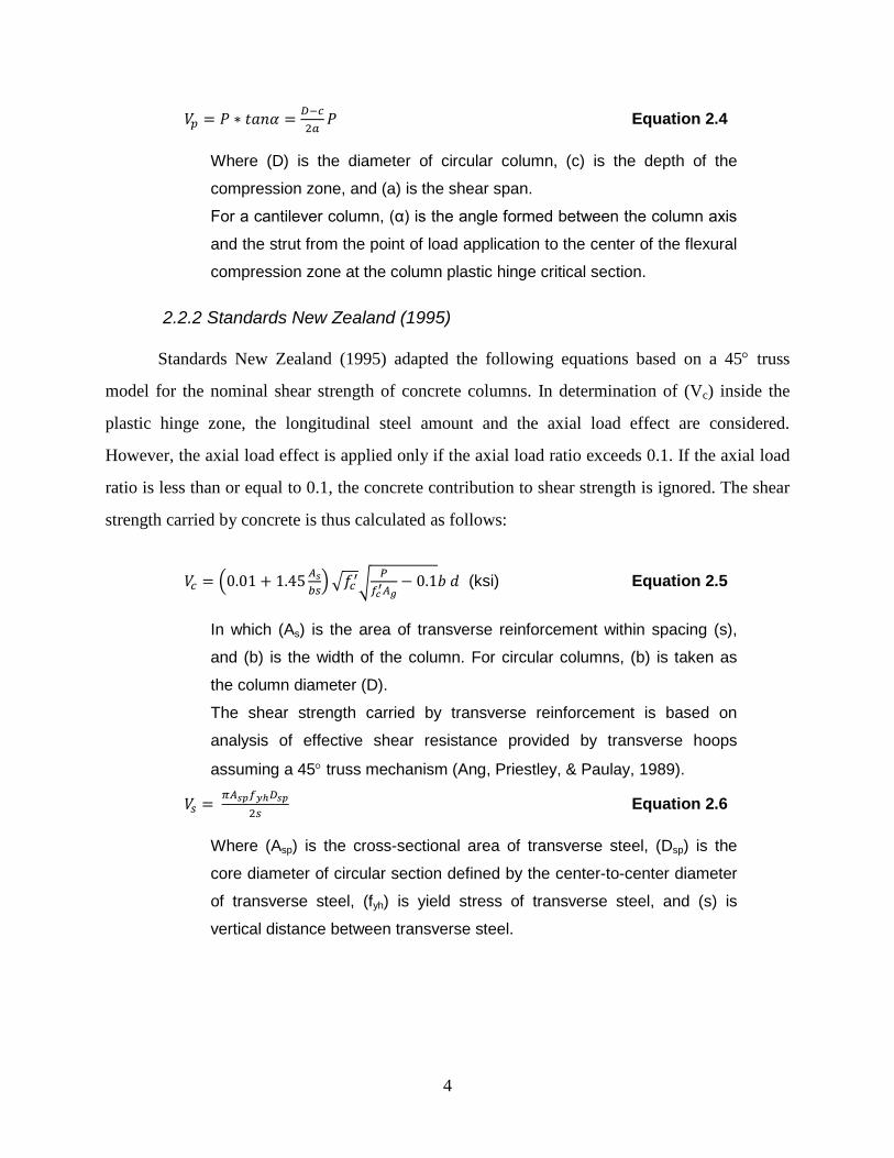
2.2.2 Standards New Zealand (1995)

Standards New Zealand (1995) adapted the following equations based on a 45° truss

model for the nominal shear strength of concrete columns. In determination of (Vc) inside the

plastic hinge zone, the longitudinal steel amount and the axial load effect are considered.

However, the axial load effect is applied only if the axial load ratio exceeds 0.1. If the axial load

ratio is less than or equal to 0.1, the concrete contribution to shear strength is ignored. The shear

strength carried by concrete is thus calculated as follows:

𝑉𝑉𝑐𝑐 = �0.01 + 1.45 𝐴𝐴𝑠𝑠

𝑏𝑏𝑠𝑠��𝑓𝑓𝑐𝑐′�

𝑃𝑃𝑓𝑓𝑐𝑐′𝐴𝐴𝑔𝑔

− 0.1𝑏𝑏 𝑑𝑑 (ksi) Equation 2.5

In which (As) is the area of transverse reinforcement within spacing (s),

and (b) is the width of the column. For circular columns, (b) is taken as

the column diameter (D).

The shear strength carried by transverse reinforcement is based on

analysis of effective shear resistance provided by transverse hoops

assuming a 45° truss mechanism (Ang, Priestley, & Paulay, 1989).

𝑉𝑉𝑠𝑠 = 𝜋𝜋𝐴𝐴𝑠𝑠𝑠𝑠𝑓𝑓𝑦𝑦ℎ𝐷𝐷𝑠𝑠𝑠𝑠2𝑠𝑠

Equation 2.6

Where (Asp) is the cross-sectional area of transverse steel, (Dsp) is the

core diameter of circular section defined by the center-to-center diameter

of transverse steel, (fyh) is yield stress of transverse steel, and (s) is

vertical distance between transverse steel.

5

2.2.3 Applied Technology Council Report ATC-32 Shear Design Equations

The design approach of Applied Technology Council Report Number ATC-32 (Nutt,

1996) also uses the combination of concrete shear resistance (Vc) and steel shear resistance (Vs).

𝑉𝑉𝑛𝑛 = 𝑉𝑉𝑐𝑐 + 𝑉𝑉𝑠𝑠 Equation 2.7

𝑉𝑉𝑠𝑠 = 𝜋𝜋𝐴𝐴ℎ𝑓𝑓𝑦𝑦ℎ𝐷𝐷′cot (𝜃𝜃)

2𝑠𝑠 Equation 2.8

𝑉𝑉𝑐𝑐 = 0.024(𝐾𝐾1 + 𝑃𝑃𝐾𝐾2𝐴𝐴𝑔𝑔

)�𝑓𝑓𝑐𝑐′(0.8 𝐴𝐴𝑔𝑔) (ksi) Equation 2.9

Where (K1) = 1.0, except in plastic hinge regions of ductile columns,

where (K1) = 0.5, and (K2) = 13.8 for compressive axial load (P) and (K2) =

3.45 for tensile axial load where (P) has the negative sign. (θ) is the angle

of the inclined flexure-shear cracks to the column axis.

2.2.4 California Department of Transportation Memo 20-4 (2010)

The California Department of Transportation (Caltrans) shear strength equations are

primarily intended as an assessment tool for determining the shear strength of existing bridge

columns, and were developed based on the Kowalsky and Priestley (2000) approach. This

approach recognizes the effect of displacement ductility on column shear strength, and shear

strength is based on the following equations for (Vc) and (Vs): 𝑉𝑉𝑠𝑠 = 𝜋𝜋𝐴𝐴𝑠𝑠𝑠𝑠𝑓𝑓𝑦𝑦ℎ𝐷𝐷𝑠𝑠𝑠𝑠

2𝑠𝑠 Equation 2.10

𝑉𝑉𝑐𝑐 = 𝑣𝑣𝑐𝑐𝐴𝐴𝑒𝑒 = 𝐹𝐹1𝐹𝐹2�𝑓𝑓𝑐𝑐′ �0.8𝐴𝐴𝑔𝑔� ≤ 0.048�𝑓𝑓𝑐𝑐′𝐴𝐴𝑔𝑔 (ksi) Equation 2.11

The shear stress of concrete (vc) is a function of the product of F1 and F2,

which are the terms related to the shear strength dependent on

displacement ductility level (𝜇𝜇) and axial load ratio (P/Ag). Displacement

ductility level is estimated by the ratio of measured maximum

displacement (∆D) to measured yield displacement (∆y) under cyclic

loading.

6

2.2.5 Joint ASCE-ACI Task Committee 426 (1973) Shear Strength Approach

Committee 426, a joint ASCE-ACI committee on shear strength of concrete members,

has produced a design equation based on the additive model (Joint ASCE-ACI Task Committee

426, 1973).

𝑉𝑉𝑛𝑛 = 𝑉𝑉𝑐𝑐 + 𝑉𝑉𝑠𝑠 Equation 2.12

The committee does not consider the influence of ductility to estimate total shear strength

of circular columns (Priestley et al., 1994).

The shear strength carried by concrete (Vc) is calculated by:

𝑉𝑉𝑐𝑐 = 𝜈𝜈𝑏𝑏 �1 + 3𝑃𝑃

𝑓𝑓𝑐𝑐′𝐴𝐴𝑔𝑔�𝐴𝐴𝑒𝑒 Equation 2.13

Where (Ae) is the effective shear area of circular column with diameter

(D), calculated as:

𝐴𝐴𝑒𝑒 = 0.8𝐴𝐴𝑔𝑔 Equation 2.14

(νb) is the nominal concrete shear stress from the following equation:

𝜈𝜈𝑏𝑏 = (0.0096 + 1.45𝜌𝜌𝑡𝑡)�𝑓𝑓𝑐𝑐′ ≤ 0.03�𝑓𝑓𝑐𝑐′ (ksi) Equation 2.15

In which (ρt) is the longitudinal tension steel ratio and it is calculated in

terms of the gross area of the column.

In order to calculate the transverse steel shear strength contribution (Vs), the committee

assumed a diagonal compression strut model at 45° to the member longitudinal axis.

𝑉𝑉𝑠𝑠 = 𝜋𝜋

2𝐴𝐴ℎ𝑓𝑓𝑦𝑦ℎ𝐷𝐷′

𝑠𝑠 Equation 2.16

In which (D’) is the spiral/hoop diameter and (Ah) is area of a single

hoop/spiral.

7

2.2.6 ACI Committee 318 (2011)

The American Concrete Institute (ACI) code ACI 318-11 considers a portion of the

design shear force to be carried by the concrete shear resistance (Vc), with the remainder carried

by transverse steel (Vs), as done by earlier codes and models. The ACI code presents the

following equation for calculating (Vc) for members subjected to combined shear, moment, and

axial compression (ACI Committee 318, 2011):

𝑉𝑉 = 𝑉𝑉𝑐𝑐 + 𝑉𝑉𝑠𝑠 Equation 2.17

𝑉𝑉𝑠𝑠 = 𝐴𝐴𝑣𝑣𝑓𝑓𝑦𝑦𝑡𝑡(sin𝛼𝛼+cos𝛼𝛼)𝑑𝑑𝑠𝑠

𝑠𝑠 Equation 2.18

𝑉𝑉𝑐𝑐 = 0.002 �1 + 𝑃𝑃2000𝐴𝐴𝑔𝑔

� 𝜆𝜆�𝑓𝑓𝑐𝑐′𝑏𝑏𝑑𝑑 (ksi) Equation 2.19

Where (P) is axial load subjected to the section, (Ag) is gross cross-

sectional area, (f’c) is concrete compressive strength, (b) is the width of

section, and (d) is the effective depth of section. (Av) is the area of

transverse reinforcement within the spacing (s), (fyt) is the yield stress of

transverse steel, (α) is the angle between inclined stirrups and

longitudinal axis of the member, and ( 𝜆𝜆) is a modification factor to

account for lightweight concrete.

2.2.7 Modified Compression Field Theory

In the 1980s, after testing different reinforced concrete members elements subjected to

pure shear, pure axial load, and a combination of shear and axial load, a theory called the

Modified Compression Field Theory (MCFT) was developed based on the Compression Field

Theory (Vecchio & Collins, 1986). The MCFT was able to accurately predict the shear behavior

of concrete members subjected to shear and axial forces. The main key of this theory is that

significant tensile stresses could exist in the concrete between the cracks, even at very high

values of average tensile strains. In addition, the value for angle θ of diagonal compressive

stresses was considered as variable compared to the fixed value of 45 assumed by the ACI code.

To simplify the process of predicting the shear strength of a section using the MCFT, the

shear stress is assumed to remain constant over the depth of the cross section, and the shear

8

strength of the section can be determined by considering the axial stress and the shear stress at

one location in the web. This was the basis of the sectional design model for shear implemented

by the AASHTO (2014) LRFD Bridge Design Specifications, based on the work of Bentz,

Vecchio, and Collins (2006).

Even though the AASHTO LRFD procedure to predict the shear strength of a section was

relatively straightforward in earlier versions of the specification, the prediction of the

contribution of concrete to shear strength of a section, which is a function of β and varying angle

θ, was required to be determined using the tables provided by AASHTO LRFD. In the most

recent version of the specifications, β and θ were defined using equations instead of the tables

approach. The factor β indicates the ability of diagonally-cracked concrete to transmit tension

and shear. The modified compression field theory was further more simplified when simple and

direct equations were developed by Bentz et al. (2006) for β and θ to replace the iterative

procedure using the tables that was implemented by earlier versions of AASHTO specifications.

These simplified equations were then used to predict the shear strength of different reinforced

concrete sections and the results were compared to those obtained from MCFT, as shown in

Figure 2.1.

Consequently the shear strength predicted by the Simplified Modified Compression Field

Theory (SMCFT) and the MCFT were compared with experimental results of various beams. It

was found that the results of the SMCFT and the MCFT were similar and both matched properly

the experimental results. In addition, the results were also compared with the ACI code, where it

was inconsistent in particular for panels with no transverse reinforcements (Bentz et al., 2006),

see Figure 2.1.

9

Figure 2.1: Ratio of Experimental to Predicted Shear Strength of Different Models Note: Graph is reproduced from data collected by Bentz et al. (2006)

Before discussing the Modified Compression Field Theory, it is important to define the

basic membrane element used to develop the approach. The reinforced concrete element is

defined to have a uniform thickness and a relatively small size. It consists of an orthogonal grid

of reinforcement with the longitudinal steel in (X) direction and the transverse steel in (Y)

direction, see Figure 2.2.

Figure 2.2: Loading and Deformation for MCFT Membrane Element

00.25

0.50.75

11.25

1.51.75

22.25

2.52.75

3

0 0.1 0.2 0.3 0.4 0.5 0.6 0.7 0.8 0.9

Vexp

/Vpr

edic

ted

ρz fy/f'c

Vexp/V(MCFT)

Vexp/V(Simplified.MCFT)

Vexp/ACI

fy

fy

fx f

νxy

νxy

νxy

νxy Y

X εx

εy

ɣxy

Loading Deformation

10

Uniform axial stresses (fx), (fy) and a uniform shear stress (νxy) are acting on the element,

causing two normal strains (εx) and (εy) in addition to a shear strain(ɣxy), see Figure 2.2. The

main target is to develop a relationship between the stresses and the strains in the member. In

order to achieve this relationship, some reasonable assumptions were made:

1. Each strain state is corresponding to one stress state.

2. Stresses and strains could be calculated in terms of average values when

taken over areas large enough to include several cracks.

3. A perfect bond exists between the steel and the concrete.

4. A uniform longitudinal and transverse steel distribution over the element.

2.2.7.1 Compatibility Conditions

Assuming a perfect bond between the concrete and the reinforcement requires that any

change in concrete strain will cause an equal change in steel strain in the same direction.

𝜀𝜀𝑐𝑐 = 𝜀𝜀𝑠𝑠 = 𝜀𝜀 Equation 2.20

By knowing the three strains εx, εy, and ɣxy, the strain in any other direction can be

calculated from the geometry of Mohr’s circle of strain, see Figure 2.3.

Figure 2.3: Mohr’s Circle of Strains

y

x

ɣ𝑥𝑥𝑥𝑥2

εy

εx

1 2

ε1 -ε2

2θ

ε

ɣ/2

11

In Figure 2.3, (ε1) represents the principal tensile strain, while (ε2) represents the principal

compressive strain. The angle of the principal direction with respect to the horizontal direction is

represented by (θ).

2.2.7.2 Equilibrium Conditions

In order to achieve equilibrium, the summation of the applied forces and the resisting

forces generated in the element should equal zero in each direction. In (x) direction (see Figure

2.2), the state of equilibrium is:

∫𝑓𝑓𝑥𝑥 𝑑𝑑𝐴𝐴 = ∫𝑓𝑓𝑐𝑐𝑥𝑥𝑑𝑑𝐴𝐴𝑐𝑐 + ∫𝑓𝑓𝑠𝑠𝑥𝑥𝑑𝑑𝐴𝐴𝑠𝑠 Equation 2.21

Where (fcx) and (Ac) are the stress in concrete and area of concrete, and

(fsx) and (As) are the stress in steel and area of steel.

Ignoring the reduction in concrete area due to the steel presence:

𝑓𝑓𝑥𝑥 = 𝑓𝑓𝑐𝑐𝑥𝑥 + 𝜌𝜌𝑠𝑠𝑓𝑓𝑠𝑠𝑥𝑥 Equation 2.22

Similarly,

𝑓𝑓𝑥𝑥 = 𝑓𝑓𝑐𝑐𝑥𝑥 + 𝜌𝜌𝑠𝑠𝑓𝑓𝑠𝑠𝑥𝑥 Equation 2.23

𝜈𝜈𝑥𝑥𝑥𝑥 = 𝜈𝜈𝑐𝑐𝑥𝑥 + 𝜌𝜌𝑠𝑠𝜈𝜈𝑠𝑠𝑥𝑥 Equation 2.24

𝜈𝜈𝑥𝑥𝑥𝑥 = 𝜈𝜈𝑐𝑐𝑥𝑥 + 𝜌𝜌𝑠𝑠𝜈𝜈𝑠𝑠𝑥𝑥 Equation 2.25

2.2.7.3 Stress-Strain Relationship

The stress-strain relationships for the concrete and the reinforcement are assumed to be

completely independent of each other. The axial stress in steel would be only a result of the axial

strain in the steel. Also, shear stresses in the steel on a plane perpendicular to the steel

longitudinal axis are assumed to be zero. Regarding the steel axial stress-axial strain relationship,

the usual bilinear relationship is assumed, see Figure 2.4.

12

𝑓𝑓𝑠𝑠 = 𝐸𝐸𝑠𝑠𝜀𝜀𝑠𝑠 ≤ 𝑓𝑓𝑥𝑥 Equation 2.26

𝜈𝜈𝑠𝑠 = 0 Equation 2.27

Where (Es) is the modulus of elasticity of steel, and (fy) is the yielding

stress in steel.

Figure 2.4: Steel Bilinear Relationship

In regard to the concrete stress-strain relationships, 30 reinforced concrete elements were

tested under different loading conditions, including pure shear, uniaxial compression, biaxial

compression, and combined shear and axial load. Longitudinal and transverse steel ratios and

concrete strength were also variables in these tests. More details are discussed in this literature

review under the experimental works section.

It was assumed that the principal strain direction in concrete (θ) and the principal stress

direction in concrete (θc) have the same angle, 𝜃𝜃𝑐𝑐 = 𝜃𝜃. However, it was observed that the

direction of the principal strain in the concrete deviated from the direction of the principal stress

in concrete, 𝜃𝜃𝑐𝑐 = 𝜃𝜃 ± 10 (Vecchio & Collins, 1986).

Although the principal compressive stress in the concrete (fc2) was found to be a function

in both the principal compressive strain (ε2) and the accompanied principal tensile strain (ε1), for

fs

fy

εs εy

𝑓𝑓𝑠𝑠𝜀𝜀𝑠𝑠

= 𝐸𝐸𝑠𝑠

𝑓𝑓𝑠𝑠 = 𝑓𝑓𝑥𝑥

13

this reason the cracked concrete under tensile strains normal to the compression is weaker than

concrete standard cylinder test, and the suggested relationship is:

𝑓𝑓𝑐𝑐2 = 𝑓𝑓𝑐𝑐2max(2𝜀𝜀2

𝜀𝜀𝑐𝑐′− (𝜀𝜀2

𝜀𝜀𝑐𝑐′)2) Equation 2.28

Where (ε’c) is the strain corresponding to the (fc2max). It is a good

observation to mention that the suggested equation is similar in behavior

to Hognestad’s concrete parabola, only differing in the maximum values;

see Figure 2.5.

Figure 2.5: Relationship between Hognestad’s Equation and MCFT Suggested Equation for the Principal Compressive Stress

In tension, it was suggested to use the linear stress-strain relationship to define the

relationship between the principal tensile stress and the principal tensile strain in concrete prior

to cracking.

𝑓𝑓𝑐𝑐1 = 𝐸𝐸𝑐𝑐𝜀𝜀1 Equation 2.29

Where (Ec) is the modulus of elasticity of concrete.

Stre

ss

Strain

Hognestad Equation

Suggested Equation

ε'c

f'c

fc2max

14

After cracking, the suggested equation is:

𝑓𝑓𝑐𝑐1 = 𝑓𝑓𝑐𝑐𝑐𝑐

1+�200𝜀𝜀1 Equation 2.30

Where (fcr) is the concrete rupture stress.

2.2.7.4 Average Stresses and Average Strains Concept

The MCFT considers average stresses and average strain across the crack. It does not

provide an approach corresponding to local stress/strain variations. The concrete tensile stresses

would be minimum value at cracks, and it would reach a value higher than the average in the

distance between the two successive cracks. The steel tensile stresses would be higher than the

average at cracks, and it would have a lower value between the cracks due to the contribution of

concrete tensile resistance.

2.2.7.5 Transmitting Shear/Tension Across Cracks

The applied stresses, (fx), (fy), and (νxy), and the internal stresses should establish a state

of equilibrium in the element. Furthermore, the internal stress at a crack plane (plane a-a) should

equal the stresses at a parallel plane in the distance between two successive cracks (plane b-b),

see Figure 2.6. The internal stresses at the crack are steel stresses (fscr), shear stresses (νc), and

minor compressive stresses (fc). The internal stresses at the uncracked plane parallel to the crack

plane are average stresses (fc1) and steel stresses (fs). In terms of average strain, the average shear

stress is zero at plane (b-b). By assuming a unit cross area along the crack, the stresses

equilibrium in (x) and (y) directions is calculated.

At (x) direction:

𝜌𝜌𝑠𝑠𝑓𝑓𝑠𝑠 sin(𝜃𝜃) + 𝑓𝑓𝑐𝑐1 sin(𝜃𝜃) = 𝜌𝜌𝑠𝑠𝑓𝑓𝑠𝑠𝑐𝑐𝑠𝑠 sin(𝜃𝜃) − 𝑓𝑓𝑐𝑐 sin(𝜃𝜃) − 𝜈𝜈𝑐𝑐cos (𝜃𝜃) Equation 2.31

At (y) direction:

𝜌𝜌𝑠𝑠𝑓𝑓𝑠𝑠 cos(𝜃𝜃) + 𝑓𝑓𝑐𝑐1 cos(𝜃𝜃) = 𝜌𝜌𝑠𝑠𝑓𝑓𝑠𝑠𝑐𝑐𝑠𝑠 cos(𝜃𝜃) − 𝑓𝑓𝑐𝑐 cos(𝜃𝜃) + 𝜈𝜈𝑐𝑐sin (𝜃𝜃) Equation 2.32

15

From Equations 2.31 and 2.32, equilibrium can’t be achieved without the shear stresses,

especially when the reinforcement at cracking (fscr) is approaching the yielding, as the concrete

contribution will then be negligible.

The shear stresses are caused due to the aggregate interlock, see Figure 2.7. Due to the

high strength of the aggregate, the concrete crack occurs along the interface of the aggregate.

The shear stress across the crack (νc) is a function in maximum aggregate size (a), crack width

(w), and the compressive stress on the crack (fc; Walraven, 1981).

Figure 2.6: State of Equilibrium for Plane (a-a) and Plane (b-b)

Walraven (1981) suggested the following equation based on experimental results.

𝜈𝜈𝑐𝑐 = 0.18νcmax +1.64𝑓𝑓𝑐𝑐 −

0.82𝑓𝑓𝑐𝑐2

𝜈𝜈𝑐𝑐𝑐𝑐𝑐𝑐𝑐𝑐 Equation 2.33

Where

𝜈𝜈𝑐𝑐𝑐𝑐𝑎𝑎𝑥𝑥 =12�−𝑓𝑓𝑐𝑐′

0.31+24 𝑤𝑤𝑐𝑐+0.63

Equation 2.34

Where (a) is the maximum aggregate size in inches, (w) is the crack width

in inches, and the concrete maximum compressive strength (f’c) is in psi.

In Equation 2.34, (f’c) should be substituted with a negative value as a

representation of compression.

b

b

a

a

a

a

b

b

fx

νxy

νxy

fy

Y

X θ

fc1

fc

νc

fscr

fscr

fs

fs

16

Figure 2.7: Aggregate Interlock

2.3 Experimental Studies

This section provides a general review of experimental studies on the behavior of circular

reinforced concrete columns under combined loading cases. The applied forces on the columns

varied between shear-moment and shear-moment and axial force. Although the main target is to

investigate the shear behavior of columns, some of the experimental studies discussed in this

section were held using a square reinforced-concrete prism, as in the case of the MCFT tests.

This prism was chosen in order to test pure shear without developing a significant moment which

might cause a shear-moment failure instead of pure shear failure.

Ang, Priestley, and Paulay (1985) tested 25 cantilever circular columns under cyclic

lateral loading and different constant axial forces (P). The circular cantilever columns were

subjected to constant axial force and a slow lateral cyclic loading with gradually increasing

displacement limits to simulate earthquake effects. The ratios of the length of the column to its

diameter were 1.5, 1.75, 2.0, and 2.5. This ratio tends also to relate the applied lateral force to the

resulting moment according to the following relationship:

17

𝑀𝑀𝑉𝑉𝐷𝐷

= 𝐿𝐿𝐷𝐷 Equation 2.35

Where (M) is the moment at the base of the cantilever, (V) is the applied

shear force, (D) is column diameter, and (L) is the effective length of the

column.

In case of a cantilever column, the effective length is the full length of the

column.

The level of axial compression force (P/(f’cAg)) were 0, 0.1, and 0.2. The volumetric

hoop reinforcement content varied between 0.0038 and 0.00102. Table 2.1 shows column details

and capacities.

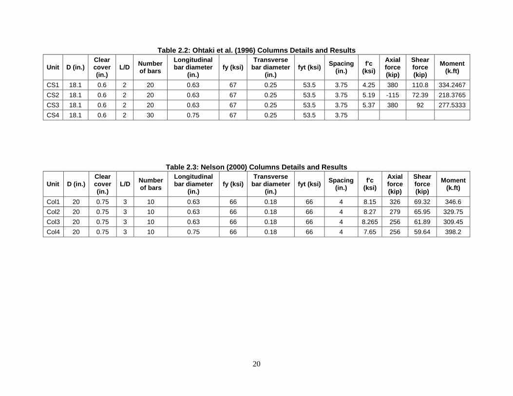
Ohtaki, Benzoni, and Priestley (1996) tested four circular reinforced-concrete columns

under cyclic lateral loading and different axial loads. The four columns were exposed to a double

bending mechanism test. The specimens (CS1, CS2, CS3, and CS4) had the same length to

diameter ratio (L/D) of 2, and also had the same reinforcement and geometrical details. The first

two columns (CS1 and CS2) were subjected to axial load ratio (P/f’cAg) of 0.35 as compression

and -0.087 as tension. The last two specimens (CS3 and CS4) were subjected to a varied axial

load calculated based on the applied lateral force. Table 2.2 describes the columns’ details and

results. Unit CS4 showed major widening of existing cracks at ductility factor μ=1.5, while the

maximum lateral forces for the other three specimens occurred at ductility factor μ=2. The tests

of the first three columns continued till μ=6 without steel fracture.

Nelson (2000) tested four circular reinforced-concrete columns to evaluate the effects of

earthquakes on “in place” bridge piers. The length to diameter ratio for the four identical

columns was 3, and the geometry and reinforcement details of these columns were similar to

Washington State Department of Transportation columns built prior to the mid-1970s. The four

columns were subjected to different lateral loading. Table 2.3 illustrates the four columns’ details

and results.

Vecchio and Collins (1986) proposed the Modified Compression Field Theory, which

deals with the reinforced cracked concrete as a new composite material as described in the

theoretical approaches presented in this literature review. In order to justify their approach, 30

reinforced concrete elements were subjected to different load combinations. Two-thirds of the

18

elements were subjected to pure shear, and one-third of the elements were subjected to a

combination of shear and axial compression/tension force. Longitudinal steel, transverse steel,

and concrete strength were also variables in this experimental program. Table 2.4 shows the

loading conditions and also shows the longitudinal and transverse steel ratio and concrete

strength for each element. The test specimens were a thin square prism (35 × 35 × 2.75 inches).

They were reinforced with two layers of welded wire mesh, with the wires parallel to the square

edge. A clear cover of 0.25 inches was provided from the longitudinal steel to the element

surface. The loads were applied using hydraulic jacks on five steel shear keys pre-casted into

each of the four edges, see Figure 2.8. The direct output of these experiments was to determine

the average strains and average stresses in the reinforcement. By knowing the external applied

forces, the cracked concrete contribution could be calculated. In Table 2.4, compression is

represented by a negative sign and tension is represented by a positive sign. Longitudinal steel

ratio and transverse steel ratio are (ρl) and (ρs), respectively.

Figure 2.8: Modified Compression Field Theory Specimen Loading Installation

Specimen 25 Shear Keys

Four Hydraulic Jacks

19

Table 2.1: Ang et al. (1985) Columns Details and Results

Unit D (in.) Clear cover (in.)

L/D Number of bars

Longitudinal bar diameter

(in.) fy (ksi)

Transverse bar

diameter (in.)

fyt (ksi) Spacing (in.)

f'c (ksi)

Axial force (kip)

Shear force (kip)

Moment (k.ft)

1 15.75 0.59 2 20 0.63 63.22 0.24 47.56 2.36 5.4375 0 72.25 189.6563 2 15.75 0.59 2 20 0.63 42.92 0.24 47.56 2.36 5.394 0 49.61 130.2263 3 15.75 0.59 2.5 20 0.63 63.22 0.24 47.56 2.36 5.22 0 62.09 203.7069 4 15.75 0.59 2 20 0.63 63.22 0.39 45.82 6.5 4.437 0 65.01 170.6513 5 15.75 0.59 2 20 0.63 63.22 0.24 47.56 1.57 4.5095 0 74.39 195.2738 6 15.75 0.59 1.5 20 0.63 63.22 0.24 47.56 2.36 4.3645 0 88.04 173.2921 7 15.75 0.59 2 20 0.63 64.96 0.24 53.94 3.15 4.2775 0 63.09 165.6113 8 15.75 0.59 2 20 0.63 64.96 0.24 53.94 1.18 4.1615 162.08 104.54 274.4175 9 15.75 0.59 2.5 20 0.63 64.96 0.24 53.94 1.18 4.335 168.82 88.3 289.27 10 15.75 0.59 2 20 0.63 64.96 0.47 48.14 4.72 4.524 176.24 101.39 266.1488 11 15.75 0.59 2 20 0.63 64.96 0.24 53.94 2.36 4.3355 168.82 91.52 240.24 12 15.75 0.59 1.5 20 0.63 64.96 0.24 53.94 1.17 4.147 80.7 118.44 233.1294 13 15.75 0.59 2 20 0.63 63.22 0.24 47.27 1.18 5.249 102.28 98.99 259.8488 14 15.75 0.43 2 9 0.94 61.48 0.24 47.27 2.36 4.8865 0 71.12 186.69 15 15.75 0.59 2 12 0.63 63.22 0.24 47.27 2.36 5.046 0 51.78 135.9225 16 15.75 0.59 2 20 0.63 63.22 0.24 47.27 2.36 4.843 94.42 83.68 219.66 17 15.75 0.59 2.5 20 0.63 63.22 0.24 47.27 2.36 4.9735 96.89 73.12 239.8945 18 15.75 0.59 2 20 0.63 63.22 0.24 47.27 2.36 5.075 98.91 113.49 297.9113 19 15.75 0.59 1.5 20 0.63 63.22 0.24 47.27 3.15 4.988 97.11 98.34 193.5659 20 15.75 0.59 1.75 20 0.63 69.89 0.24 47.27 3.15 5.3215 181.41 109.4 251.2553 21 15.75 0.59 2 20 0.63 63.22 0.24 47.27 3.15 4.814 0 60.8 159.6 22 15.75 0.59 2 20 0.63 63.22 0.39 44.95 8.66 4.4805 0 64.03 168.0788 23 15.75 0.59 2 20 0.63 63.22 0.47 48.14 6.3 4.6835 0 74.75 196.2188 24 15.75 0.59 2 20 0.63 63.22 0.39 44.95 4.33 4.7995 0 76.54 200.9175

20

Table 2.2: Ohtaki et al. (1996) Columns Details and Results

Unit D (in.) Clear cover (in.)

L/D Number of bars

Longitudinal bar diameter

(in.) fy (ksi)

Transverse bar diameter

(in.) fyt (ksi) Spacing

(in.) f'c

(ksi) Axial force (kip)

Shear force (kip)

Moment (k.ft)

CS1 18.1 0.6 2 20 0.63 67 0.25 53.5 3.75 4.25 380 110.8 334.2467 CS2 18.1 0.6 2 20 0.63 67 0.25 53.5 3.75 5.19 -115 72.39 218.3765 CS3 18.1 0.6 2 20 0.63 67 0.25 53.5 3.75 5.37 380 92 277.5333 CS4 18.1 0.6 2 30 0.75 67 0.25 53.5 3.75

Table 2.3: Nelson (2000) Columns Details and Results

Unit D (in.) Clear cover (in.)

L/D Number of bars

Longitudinal bar diameter

(in.) fy (ksi)

Transverse bar diameter

(in.) fyt (ksi) Spacing

(in.) f'c

(ksi) Axial force (kip)

Shear force (kip)

Moment (k.ft)

Col1 20 0.75 3 10 0.63 66 0.18 66 4 8.15 326 69.32 346.6 Col2 20 0.75 3 10 0.63 66 0.18 66 4 8.27 279 65.95 329.75 Col3 20 0.75 3 10 0.63 66 0.18 66 4 8.265 256 61.89 309.45 Col4 20 0.75 3 10 0.75 66 0.18 66 4 7.65 256 59.64 398.2

21

Table 2.4: Modified Compression Field Theory Experimental Program

Panel Loading ratio ν-fx-fy ρl fy (ksi) ρs fyt (ksi) f'c (ksi) νu (ksi) (failure)

PV1 1:00:00 0.0179 70.035 0.0168 70.035 -5.0025 1.1629 PV2 1:00:00 0.0018 62.06 0.0018 62.06 -3.4075 0.1682 PV3 1:00:00 0.0048 95.99 0.0048 95.99 -3.857 0.44515 PV4 1:00:00 0.0106 35.09 0.0106 35.09 -3.857 0.41905 PV5 1:00:00 0.0074 90.045 0.0074 90.045 -4.1035 0.6148 PV6 1:00:00 0.0179 38.57 0.0179 38.57 -4.321 0.65975 PV7 1:00:00 0.0179 65.685 0.0179 65.685 -4.495 0.98745 PV8 1:00:00 0.0262 66.99 0.0262 66.99 -4.321 0.96715 PV9 1:00:00 0.0179 65.975 0.0179 65.975 -1.682 0.5423 PV10 1:00:00 0.0179 40.02 0.01 40.02 -2.1025 0.57565 PV11 1:00:00 0.0179 34.075 0.0131 34.075 -2.262 0.5162 PV12 1:00:00 0.0179 68.005 0.0045 68.005 -2.32 0.45385 PV13 1:00:00 0.0179 35.96 0 0 -2.639 0.29145 PV14 1:00:00 0.0179 65.975 0.0179 65.975 -2.958 0.7598 PV15 00:-1:00 0.0074 36.975 0.0074 36.975 -3.1465 -2.842 PV16 1:00:00 0.0074 36.975 0.0074 36.975 -3.1465 0.3103 PV17 00:-1:00 0.0074 36.975 0.0074 36.975 -2.697 -3.0885 PV18 1:00:00 0.0179 62.495 0.0032 59.74 -2.8275 0.4408 PV19 1:00:00 0.0179 66.41 0.0071 43.355 -2.755 0.57275 PV20 1:00:00 0.0179 66.7 0.0089 43.065 -2.842 0.6177 PV21 1:00:00 0.0179 66.41 0.013 43.79 -2.8275 0.72935 PV22 1:00:00 0.0179 66.41 0.0152 60.9 -2.842 0.88015 PV23 1:-0.39:-0.39 0.0179 75.11 0.0179 75.11 -2.9725 1.28615 PV24 1:-0.83:-0.83 0.0179 71.34 0.0179 71.34 -3.451 1.1513 PV25 1:-0.69:-0.69 0.0179 67.57 0.0179 67.57 -2.784 1.3224 PV26 1:00:00 0.0179 66.12 0.0101 67.135 -3.0885 0.78445 PV27 1:00:00 0.0179 64.09 0.0179 64.09 -2.9725 0.92075 PV28 1:0.32:0.32 0.0179 70.035 0.0179 70.035 -2.755 0.841 PV29 Changing 0.0179 63.945 0.0089 46.98 -3.1465 0.85115 PV30 1:00:00 0.0179 63.365 0.0101 68.44 -2.7695 0.74385

22

Chapter 3: Present Formulation

3.1 Overview

This section provides the proposed approaches to generate the interaction domain

(moment-shear force-axial force) for non-prestressed reinforced concrete columns. The first

approach is based on the SMCFT and AASHTO (2014) LRFD Bridge Construction

Specifications.

3.2 AASHTO (2014) LRFD Approach

The present procedure is based on the SMCFT originally developed by Bentz, Vecchio,

and Collins (2006), and adopted by AASHTO (2014) LRFD specifications. This theory was

derived based on the MCFT developed earlier by Vecchio and Collins (1986). In this section,

shear equations used in this study are presented and specialized for the present application of

non-prestressed circular reinforced concrete columns.

3.2.1 Minimum Transverse Steel

The following empirical equation is adopted to signify the minimum transverse

reinforcement allowed by AASHTO (2014):

𝐴𝐴𝑣𝑣 ≥ .0316�𝑓𝑓𝑐𝑐′

𝑏𝑏𝑣𝑣𝑠𝑠𝑓𝑓𝑦𝑦

(𝐴𝐴𝑣𝑣 ≥ .083�𝑓𝑓𝑐𝑐′𝑏𝑏𝑣𝑣𝑠𝑠𝑓𝑓𝑦𝑦

) (AASHTO, 2014) Equation 3.1

Where:

Av = area of transverse reinforcement within spacing (s) in in2 (mm2)

f’c = concrete compressive capacity in ksi (MPa)

bv = effective web width taken as the minimum web width, measured

parallel to the neutral axis, between the tensile resultant and compressive

force due to flexure, or for circular sections, it is taken as the diameter of

the section in inches (mm); see Figure 3.1.

s = spacing of transverse reinforcement in inches (mm)

fy = yield strength in transverse steel in ksi (MPa)

23

A minimum amount of transverse reinforcement is necessary to control the growth of

shear diagonal cracking. Based on this equation, there are two cases of analysis as described

below.

3.2.2 Shear Resistance

The section nominal shear capacity is determined as the summation of concrete shear

contribution and transverse steel shear contribution. Concrete shear contribution is a function in

the effective shear area (bv*dv), concrete strength, and (β), which indicates the ability of the

diagonally-cracked concrete to transmit shear along its axis. Transverse steel shear contribution

depends on the transverse steel yielding strength, area of transverse steel, the angle of cracking

(θ), and the angle of inclination of transverse reinforcement to the longitudinal axis (α).

𝑉𝑉𝑛𝑛 = 𝑉𝑉𝑐𝑐 + 𝑉𝑉𝑠𝑠 (AASHTO, 2014) Equation 3.2

In which

𝑉𝑉𝑐𝑐 = .0316β�𝑓𝑓𝑐𝑐′𝑏𝑏𝑣𝑣𝑑𝑑𝑣𝑣 (𝑉𝑉𝑐𝑐 = β�𝑓𝑓𝑐𝑐′𝑏𝑏𝑣𝑣𝑑𝑑𝑣𝑣) (AASHTO, 2014) Equation 3.3

𝑉𝑉𝑠𝑠 = 𝜋𝜋2𝐴𝐴𝑣𝑣𝑓𝑓𝑦𝑦𝑑𝑑𝑣𝑣(𝑐𝑐𝑐𝑐𝑡𝑡𝜃𝜃+𝑐𝑐𝑐𝑐𝑡𝑡𝛼𝛼)𝑠𝑠𝑠𝑠𝑛𝑛𝛼𝛼

𝑠𝑠 (AASHTO, 2014) Equation 3.4

Where

Vc = concrete shear strength that relies on the tensile stresses in concrete

in ksi (MPa)

Vs = steel shear strength that relies on the tensile stresses in transverse

steel in ksi (MPa)

dv = effective shear depth taken as the distance, measured perpendicular

to the neutral axis, between the tensile resultant and compressive force

due to flexure. It needs not be taken to be less than the greater of 0.9de or

0.72h in inches (mm); see Figure 3.1.

β = factor indicating ability of diagonally-cracked concrete to transmit

tension and shear

𝜃𝜃 = angle of inclination of diagonal compressive stresses (˚)

𝑡𝑡 = angle of inclination of transverse reinforcement to longitudinal axis (˚);

see Figure 3.2.

24

Figure 3.1: Illustration of bv and dv Parameters

Figure 3.2: Illustration of Angle (θ) and Angle (α)

3.2.3 Determination of β and θ

In the case that the transverse steel is more than the minimum transverse steel required by

AASHTO (2014) LRFD Bridge Construction Specifications (see Equation 3.1), β and θ are

calculated based on the longitudinal axial strain at the centroid of tensile steel (εs). This is

identified as Case 1 in this study:

β = 4.8

1+750𝜀𝜀𝑠𝑠 (β = 0.4

1+750𝜀𝜀𝑠𝑠) (AASHTO, 2014) Equation 3.5

𝜃𝜃 = 29(𝑑𝑑𝑑𝑑𝑑𝑑𝑑𝑑𝑑𝑑𝑑𝑑) + 3500𝜀𝜀𝑠𝑠 ≤ 75˚ (AASHTO, 2014) Equation 3.6

Note that Equation 3.5 is for the kip-in. units (SI units) system.

θ

α

de dv

bv=D

25

In the case that the transverse steel is less than the minimum transverse steel required by

AASHTO (2014) LRFD specifications (see Equation 3.1), β and 𝜃𝜃 are calculated based on the

longitudinal axial strain at the centroid of tensile steel (𝜀𝜀𝑠𝑠) and crack spacing parameter (sxe).

This is identified as Case 2 in this study:

β = 4.8

1+750𝜀𝜀𝑠𝑠

5139+𝑠𝑠𝑐𝑐𝑥𝑥

(β = 0.41+750𝜀𝜀𝑠𝑠

13001000+𝑠𝑠𝑐𝑐𝑥𝑥

) (AASHTO, 2014) Equation 3.7

𝜃𝜃 = (29(𝑑𝑑𝑑𝑑𝑑𝑑𝑑𝑑𝑑𝑑𝑑𝑑) + 3500𝜀𝜀𝑠𝑠) (AASHTO, 2014) Equation 3.8

𝑠𝑠𝑥𝑥𝑒𝑒 = 𝑠𝑠𝑥𝑥1.38

𝑎𝑎𝑔𝑔+0.63 (𝑠𝑠𝑥𝑥𝑒𝑒 = 𝑠𝑠𝑥𝑥

35𝑎𝑎𝑔𝑔+16

) ≥ 12 𝑖𝑖𝑡𝑡 (AASHTO, 2014) Equation 3.9

sx = the lesser of dv or the vertical distance between horizontal layers of

longitudinal crack control reinforcement in inches (mm)

ag = maximum aggregate size in inches (mm); has to equal zero when

𝑓𝑓’𝑐𝑐 ≥ 10 𝑘𝑘𝑠𝑠𝑖𝑖 (69 𝑀𝑀𝑃𝑃𝑡𝑡)

Note that Equations 3.7 and 3.9 are for the kip-in. units (SI units) system.

If the section has transverse steel less than the minimum transverse steel defined by

AASHTO (2014) LRFD Specifications (Case 2), the specification allows for checking the shear

contribution due to aggregate size (1.38/(ag+0.63)) and longitudinal steel (Sx). However, if there

is enough longitudinal steel and the aggregate size is efficient, (Sxe) must not be less than 12 inches so the factor � 51

39+𝑠𝑠𝑐𝑐𝑥𝑥� ≤ 1.

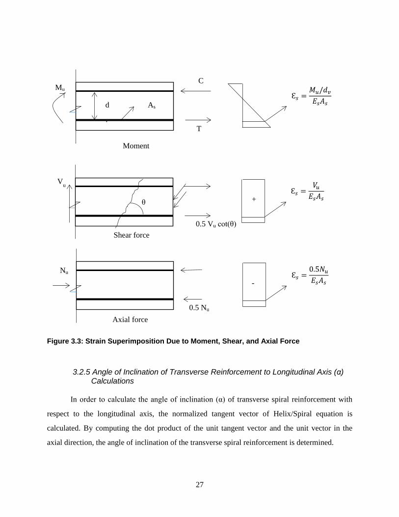
3.2.4 Calculation of Longitudinal Axial Strain (𝜺𝜺𝒔𝒔)

Longitudinal axial strain (𝜀𝜀𝑠𝑠) is calculated based on the superimposed effect of the forces

in the tension side of the section, as follows (see Figure 3.3):

𝜀𝜀𝑠𝑠 = |𝑀𝑀|𝑑𝑑𝑣𝑣+0.5𝑁𝑁+𝑉𝑉

𝐴𝐴𝑠𝑠𝐸𝐸𝑠𝑠 (AASHTO, 2014) Equation 3.10

𝜀𝜀𝑠𝑠 must not exceed 0.006 to maintain a reasonable crack widening.

If the value of (𝜀𝜀𝑠𝑠) computed from this case is negative, which means the section is under

compression, the concrete rigidity is added to the denominator:

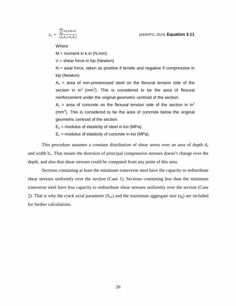
26

𝜀𝜀𝑠𝑠 = |𝑀𝑀|𝑑𝑑𝑣𝑣+0.5𝑁𝑁+𝑉𝑉

(𝐴𝐴𝑠𝑠𝐸𝐸𝑠𝑠+𝐴𝐴𝑐𝑐𝐸𝐸𝑐𝑐) (AASHTO, 2014) Equation 3.11

Where

M = moment in k.in (N.mm)

V = shear force in kip (Newton)

N = axial force, taken as positive if tensile and negative if compressive in

kip (Newton)

As = area of non-prestressed steel on the flexural tension side of the

section in in2 (mm2). This is considered to be the area of flexural

reinforcement under the original geometric centroid of the section.

Ac = area of concrete on the flexural tension side of the section in in2

(mm2). This is considered to be the area of concrete below the original

geometric centroid of the section.

Es = modulus of elasticity of steel in ksi (MPa).

Ec = modulus of elasticity of concrete in ksi (MPa).

This procedure assumes a constant distribution of shear stress over an area of depth dv

and width bv. That means the direction of principal compressive stresses doesn’t change over the

depth, and also that shear stresses could be computed from any point of this area.

Sections containing at least the minimum transverse steel have the capacity to redistribute

shear stresses uniformly over the section (Case 1). Sections containing less than the minimum

transverse steel have less capacity to redistribute shear stresses uniformly over the section (Case

2). That is why the crack axial parameter (Sxe) and the maximum aggregate size (ag) are included

for further calculations.

27

Figure 3.3: Strain Superimposition Due to Moment, Shear, and Axial Force

3.2.5 Angle of Inclination of Transverse Reinforcement to Longitudinal Axis (α) Calculations

In order to calculate the angle of inclination (α) of transverse spiral reinforcement with

respect to the longitudinal axis, the normalized tangent vector of Helix/Spiral equation is

calculated. By computing the dot product of the unit tangent vector and the unit vector in the

axial direction, the angle of inclination of the transverse spiral reinforcement is determined.

Ɛ𝑠𝑠 =𝑀𝑀𝑢𝑢/𝑑𝑑𝑣𝑣𝐸𝐸𝑠𝑠𝐴𝐴𝑠𝑠

C

T

Mu

Ɛ𝑠𝑠 =

𝑉𝑉𝑢𝑢𝐸𝐸𝑠𝑠𝐴𝐴𝑠𝑠

0.5 Vu cot(θ)

Vu

θ

As

Ɛ𝑠𝑠 =

0.5𝑁𝑁𝑢𝑢𝐸𝐸𝑠𝑠𝐴𝐴𝑠𝑠

0.5 Nu

Nu

+

-

Moment

Shear force

Axial force

d

v

28

A circular helix of radius (Dr/2; core radius) and pitch/spacing (s) is described by the

following parameterization, see Figure 3.4 for helix 3D plotting:

𝑥𝑥(𝑑𝑑) = 𝐷𝐷𝑐𝑐

2cos(𝑑𝑑) Equation 3.12

𝑦𝑦(𝑑𝑑) = 𝐷𝐷𝑐𝑐2

sin(𝑑𝑑) Equation 3.13

𝑧𝑧(𝑑𝑑) = 𝑠𝑠2𝜋𝜋𝑑𝑑 Equation 3.14

Tangent vector = < −𝐷𝐷𝑐𝑐2

sin(𝑑𝑑) , 𝐷𝐷𝑐𝑐2

cos(𝑑𝑑) , 𝑠𝑠2𝜋𝜋

>

||Tangent vector|| = ��𝐷𝐷𝑐𝑐2�2

+ � 𝑠𝑠2𝜋𝜋�2

Unit tangent vector (𝑡𝑡) = Tangent vector || Tangent vector||

Unit vector in the axial direction of the column (𝑘𝑘) = <0, 0, 1>

The dot product of < 𝑘𝑘 >. < 𝑡𝑡 > = 𝑠𝑠/2𝜋𝜋

��𝐷𝐷𝑐𝑐2 �2+� 𝑠𝑠2𝜋𝜋�

2 = 1 ∗ 1 ∗ cos𝑡𝑡.

In the case that the section contains transverse reinforcement of hoops, the angle of

inclination of transverse steel to the axial direction (𝑡𝑡) is 90°. For sections that contain spiral

transverse reinforcement:

𝑡𝑡 = cos−1( 𝑠𝑠/2𝜋𝜋

��𝐷𝐷𝑐𝑐2 �2+� 𝑠𝑠2𝜋𝜋�

2)

3.2.6 Effective Number of Legs of Transverse Steel in Shear Resistance Calculation

Most design codes assume two legs of transverse steel are resisting the shear force, taking

Av=2Ah for circular and rectangular sections. However, a new value for the effective number of

legs in circular sections has been defined based on a 45° angle of diagonal cracking (Ang et al.,

1989). The new assigned value equals to (π/2) as an average integrated value along a 45° crack,

see Figure 3.5 for the geometrical details.

29

Figure 3.4: Helix/Spiral 3D Plot

Figure 3.5: Shear Carried by Transverse Steel in Circular Column

Dr/2 s

s

45

θ

θ

Force (i)

dx dy

r.dθ

√2 𝑑𝑑𝑦𝑦 Elevation

Plan

Infinitesimal Element

Y

X D’

r

30

The average total force in the transverse steel over the crack length is the summation of

each hoop force divided by the length of the crack (√2 𝐷𝐷′)—in other words, it is the integration

of the forces over the length of the crack.

𝑉𝑉𝑠𝑠 = ∫ 𝐹𝐹𝑐𝑐𝑠𝑠𝑐𝑐𝑒𝑒𝑠𝑠(𝑠𝑠).√2 𝑑𝑑𝑥𝑥𝐷𝐷′0

√2 𝐷𝐷′ Equation 3.15

Where

Vs = transverse steel shear resistance.

Force (i) = the transverse steel force in the hoop at the crack location, see

Figure 3.5.

In each single hoop, the force in (Y) direction is calculated as follows:

𝐹𝐹𝐹𝐹𝑑𝑑𝐹𝐹𝑑𝑑(𝑖𝑖) = 2𝐴𝐴𝑠𝑠ℎ𝑓𝑓𝑥𝑥sin (𝜃𝜃) Equation 3.16

Where

Ash= transverse steel single hoop area

Substitute in Equation 3.15,

𝑉𝑉𝑠𝑠 = ∫ 2𝐴𝐴𝑠𝑠ℎ𝑓𝑓𝑦𝑦sin (𝜃𝜃).√2 𝑑𝑑𝑥𝑥𝐷𝐷′0

√2 𝐷𝐷′ Equation 3.17

But from geometry, 𝑑𝑑𝑦𝑦 = 𝑑𝑑𝑑𝑑𝜃𝜃sin (𝜃𝜃) Equation 3.18

𝐷𝐷’ = 2𝑑𝑑 Equation 3.19

Then, 𝑉𝑉𝑠𝑠 = 2∫ 2𝐴𝐴𝑠𝑠ℎ𝑓𝑓𝑥𝑥𝑠𝑠𝑖𝑖𝑡𝑡2(𝜃𝜃).𝑑𝑑𝜃𝜃𝜋𝜋/2

0 Equation 3.20

𝑉𝑉𝑠𝑠 = 2∫ 2𝐴𝐴𝑠𝑠ℎ𝑓𝑓𝑥𝑥1−cos (2𝜃𝜃)

2𝑑𝑑𝜃𝜃𝜋𝜋/2

0 Equation 3.21

𝑉𝑉𝑠𝑠 = 2𝐴𝐴𝑠𝑠ℎ𝑓𝑓𝑥𝑥 �𝜃𝜃2− 𝑠𝑠𝑠𝑠𝑛𝑛2𝜃𝜃

2�0

𝜋𝜋/2 Equation 3.22

𝑉𝑉𝑠𝑠 = 𝜋𝜋2𝐴𝐴𝑠𝑠ℎ𝑓𝑓𝑥𝑥 Equation 3.23

31

Chapter 4: Implementation

4.1 Overview

As a general guideline for our numerical solution approach, the mathematical procedure

is based on finding the shear capacity of the section corresponding to a certain level of moment

and axial force. By applying this procedure for the full range of moments under a constant axial

force, we were able to develop a 2D moment-shear force interaction diagram under a specific

axial force. The collection of all the 2D interaction diagrams yielded a 3D interaction diagram of

a circular reinforced-concrete cross section.

4.2 Input Parameters

In order to apply our numerical approach, a set of parameters needs to be pre-defined.

These parameters could be classified into material properties, reinforcement, and geometry.

1. Material Properties: Yielding strength for longitudinal (fy) and transverse

bars (fyh), concrete compressive strength (f’c), and modulus of elasticity of

steel (Es) were defined as the material properties. Modulus of elasticity of

concrete (Ec) was calculated based on the concrete compressive strength

𝐸𝐸𝑐𝑐 = 57�𝑓𝑓′𝐹𝐹 (𝐸𝐸𝑐𝑐 = 4700�𝑓𝑓′𝐹𝐹 ), where f’c is in psi (MPa) units and Ec

is in ksi (MPa) units.

2. Reinforcement Properties: The reinforcement parameters are the number

of longitudinal bars, cross section dimensions of longitudinal bars

(diameter, area [As]), cross section dimensions of transverse bars

(diameter, area [Av]), the type of transverse reinforcement (hoop or spiral),

and the transverse bar spacing (s).

3. Geometric Properties: Circular cross section diameter (d) and clear cover

(cc) were the two direct geometrical parameters used in this analysis.

Effective shear depth (dv) and effective web width (bv) are two indirect

geometrical parameters needed to calculate steel and concrete shear

capacities.

32

4.3 Effective Shear Area

In our case of reinforced-concrete circular sections, it was agreed to use the effective web

width as the diameter of the circular section per the AASHTO (2014) requirements, although it is

less conservative, as it increases the value of concrete shear capacity (Vc). It also seems to

contradict the main definition of effective web width as the minimum web width of the section.

However, according to the specifications, circular members typically have the longitudinal steel

uniformly distributed around the perimeter of the section, and when the member cracks, the

highest shear stresses occur near the mid-depth of the cross section. It is for this reason the

effective web width was be taken by AASHTO to be the diameter. For the centroid location of

the tensile force, the neutral axis of the cross section is assumed by AASHTO LRFD

specifications to be always across the middle of the section at a depth equals d/2. This

assumption was expected to decrease the moment capacity of the section, which is more

conservative; see Figure 3.1.

4.3.1 Effective Shear Depth Calculation (dv)

dv = Max{0.72h,0.9de,dv}

de = the distance from the upper compressive fiber to the resultant of

tensile forces in inches (mm)

𝑑𝑑𝑒𝑒 = 𝑑𝑑/2 + 𝑑𝑑𝑠𝑠/𝜋𝜋 (AASHTO, 2014) Equation 4.1

d = diameter of section in inches (mm)

dr = diameter of the circle passing through the centers of the longitudinal

bars in inches (mm)

The second term in Equation 4.1 represents the geometric centroid of a semicircular ring.

dv = distance between the compressive resultant point of action and the

tensile resultant point of action in inches (mm). According to AASHTO

(2014) specification (dv) could be approximated as follows by assuming

ALL the tensile steel to yield:

𝑑𝑑𝑣𝑣 = 𝑀𝑀𝐴𝐴𝑠𝑠𝑓𝑓𝑦𝑦

(AASHTO, 2014) Equation 4.2

33

4.4 Analysis Procedure

Under a constant axial compressive force (N), the moment-shear interaction diagram is

determined by increasing the value of the moment from zero to the ultimate confined moment

capacity corresponding to zero-shear, while solving for the total shear capacity under every moment

step. The ultimate confined moment capacity at zero-shear and axial force (N) is readily available

from the procedure developed earlier by Abd El-Fattah, Rasheed, and Esmaeily (2011). At a zero

moment value, the shear capacity is estimated first based on a 45° angle of shear crack (cot θ=1) and

a concrete strength based on (Ɛ𝑠𝑠 = 0.00457, β= 1.084). This shear capacity is then used along with

the axial force (N) to determine (Ɛ𝑠𝑠), based on Equation 3.10. The longitudinal strain at the centroid

of tensile reinforcement (Ɛ𝑠𝑠) is then used to compute θ and β based on Equations 3.6 and 3.10 or

Equations 3.7, 3.8, and 3.9 for sections having less transverse steel than minimum transverse steel

defined by AASHTO (2014) LRFD specifications, see Equation 3.1. The concrete and steel shear

capacities are determined next using Equations 3.3 and 3.4, and totaled using Equation 3.2 to update

the section shear strength (V). If that value is equal to the initially estimated shear capacity, then

convergence is achieved. Otherwise, the updated shear capacity is used to reiterate until convergence

of the newly updated shear capacity, see Figure 4.2. Once the new moment step is input, the shear

capacity of the previous step, along with (N), is used to compute (Ɛ𝑠𝑠), and iterations are resumed

until the new shear capacity convergences. The interaction diagram is concluded when the moment

step reaches the ultimate confined moment capacity corresponding to zero-shear, see Figure 4.1.

Figure 4.1: Moment-Shear Interaction Diagram Under a Constant Axial Compression Force

Shea

r

Moment

Capacity based on first limit

Standard procedure

Capacity based on third limit

Maximum moment capacity at zero shear

34

Figure 4.2: Flow Chart of Present Procedure (Case 1: Sections with More than Minimum Transverse Steel).

35

4.4.1 Limits of Constraints

The value of the shear capacity (V) should satisfy five other limits according to

AASHTO (2014) LRFD Bridge Construction Specifications.

1. The first limit is [𝑀𝑀 ≥ 𝑉𝑉𝑑𝑑𝑣𝑣]. If this limit is not achieved at a moment step,

the iteration should be repeated with an initial value of moment (M) equals

to (V.dv).

2. The second limit is [Ɛ𝑠𝑠 ≤ 0.006]. If not, (Ɛs) is set to 0.006, and the shear

capacity (V) is directly calculated. 3. The third limit or the yield limit is [𝐴𝐴𝑠𝑠𝑓𝑓𝑥𝑥 ≥

𝑀𝑀𝑑𝑑𝑣𝑣

+ 𝑁𝑁2

+ 𝑉𝑉 cot(𝜃𝜃) −

0.5𝑉𝑉𝑠𝑠 cot(𝜃𝜃)]. If not, the shear capacity value (V) should be reduced

according to this limit. 4. The forth limit is the spacing limit; if [𝑣𝑣𝑢𝑢 = 𝑉𝑉

𝑏𝑏𝑣𝑣𝑑𝑑𝑣𝑣< 0.125𝑓𝑓𝑐𝑐′], then the max

spacing equals 0.8 ∗ 𝑑𝑑𝑣𝑣 ≤ 24 𝑖𝑖𝑡𝑡. (609.6 𝑚𝑚𝑚𝑚). And if [𝑣𝑣𝑢𝑢 = 𝑉𝑉𝑏𝑏𝑣𝑣𝑑𝑑𝑣𝑣

≥

0.125𝑓𝑓𝑐𝑐′], then the max spacing equals 0.4 ∗ 𝑑𝑑𝑣𝑣 ≤ 12 𝑖𝑖𝑡𝑡. (304.8 𝑚𝑚𝑚𝑚). If

this limit is not achieved, the analysis is stopped, warning the user to

decrease the spacing to satisfy this limit.

5. The fifth limit is [𝑉𝑉 ≤ 0.25 ∗ 𝑓𝑓′𝐹𝐹 ∗ 𝑑𝑑𝑣𝑣 ∗ 𝑏𝑏𝑣𝑣], otherwise the shear value is

set to be [𝑉𝑉 = 0.25 ∗ 𝑓𝑓′𝐹𝐹 ∗ 𝑑𝑑𝑣𝑣 ∗ 𝑏𝑏𝑣𝑣].

The first limit controls when the moment value approaches the point of zero moment (e.g.

simple beam support). The specification assigned a moment value equal to V.dv over the length

where moment is negligible. This limit causes a horizontal line at the top of shear-moment

interaction diagram, see Figure 4.1. The second limit illustrates that the tensile strain of

longitudinal steel on the tension side should not exceed an excessive value in order to keep

cracks width within a reasonable value to effectively transmit tension along the member. The

third limit formula could be derived from Figure 4.3 by taking the moment summation around

point (o), and it aims to ensure that the force in the longitudinal steel is equal to or less than the

maximum force that could be carried by the steel. The fourth limit is to minimize the diagonal

shear crack width by having enough transverse steel within the spacing (s) to resist shear

36

stresses. The fifth limit was intended to ensure that the concrete strut will not crush before the

transverse steel yields.

Figure 4.3: Derivation of the Yielding Stress Limit

There are two more conditions that cause the AASHTO (2014) LRFD specifications to

consider the section invalid if one of them is met, and new section properties are then

recommended.

The first condition is in the case of sections having less than the minimum transverse

steel defined by AASHTO (2014) LRFD specifications, see Equation 3.1. If the section doesn’t

have enough longitudinal steel to control cracks along its diameter according to the following

equation, the section is considered invalid:

𝐴𝐴𝑙𝑙𝑎𝑎𝑥𝑥𝑒𝑒𝑠𝑠 = 0.003𝑏𝑏𝑣𝑣𝑠𝑠𝑥𝑥 Equation 4.3

Where (Alayer) is the area of longitudinal steel in each layer of

reinforcement (in2). More longitudinal bars or bigger bars are then

recommended to control cracks.

The second condition is to make sure that there is a clear yielding zone in the steel stress-

strain curve. Thus, the steel yielding strength should not exceed 100 ksi, see Figure 4.4. This

value was verified for both prestressed and non-prestressed members for nonseismic applications

(Shahrooz, Miller, Harries, & Russell, 2011).

M M

V

V

N N

θ

37

Figure 4.4: Yielding Zone for Different Yielding Strength

Stre

ss

Strain

fy >100 ksi

fy <100 ksi

ε(yield)

38

Chapter 5: Experimental Verification

5.1 Overview

The proposed formulations were verified against a large pool of experimental data

performed by different researchers in different countries. In this section, a full database and the

experimental parameters for the sections are presented in Tables 5.3 to 5.33. Full database

comparisons against experimental studies and interaction diagrams are shown in Chapter 7.

Randomly selected sections are discussed in detail with necessary comments in this chapter. A

comparison against the experimental studies and another against Response 2000 were applied in

this chapter to verify the accuracy of the proposed methods. Response 2000 is a structural tool

that was developed based on AASHTO (1999) LRFD Bridge Construction Specifications and the

MCFT, and it also predicts shear strength and moment-shear interaction diagrams at specific

levels of axial loads.

5.2 Database Criteria

The database presented in this chapter represents a large different pool of experimental

studies. However, the selected sections in this study had to match certain criteria defined by

AASHTO (2014) LRFD Specifications and the research goals regarding loads, geometry, and

materials. The first condition regarding loads is that the axial force applied on the section should

be compressive force 𝑁𝑁 ≤ 0 𝑘𝑘𝑖𝑖𝑘𝑘𝑠𝑠 (assuming negative sign for compression); the interaction

diagrams in this study were generated for the axial compression forces range. In terms of

geometry, the transverse steel spacing must not exceed the maximum spacing defined by

AASHTO LRFD Specifications, see Section 4.4.1. The last condition is that the steel yielding

strength should not exceed 100 ksi in order to have a clear yielding zone.

5.3 Comparisons Against Experimental Studies

Fourteen different sections were randomly selected from the database to be discussed in

this chapter (see Table 5.1). Table 5.2 shows their material and geometrical properties. The table

also shows the applied constant axial force, and moment and shear failure values. The ratio

39

(La/D) in the table is the ratio of the effective column length to its diameter, and it tends to relate

the applied lateral force to the resulting moment according to the following relationship.

𝑀𝑀

𝑉𝑉𝐷𝐷= 𝐿𝐿𝑐𝑐

𝐷𝐷 Equation 5.1

Where (M) is the moment at the base of the cantilever, (V) is the applied

shear force, (D) is column diameter, and (L) is the effective length of the

column.

In case of a cantilever column, the effective length is the full length of the

column.

Table 5.1: Selected Sections

No. Reference Unit

1 Arakawa, He, Arai, and Mizoguchi (1987) No.16 2 Ang, Priestley, and Paulay (1985) UNIT21 3 Roeder, Graff, Soderstrom, and Yoo (2001) C1 4 Ranf, Eberhard, and Stanton (2006) SpecimenC2 5 Zahn, Park, and Priestley (1986) No.5 6 Pontangaroa, Priestley, and Park (1979) Unit4 7 Nelson (2000) Col4 8 Lehman and Moehle (2000) No.430 9 Kunnath, El-Bahy, Taylor, and Stone (1997) A8 10 Moyer and Kowalsky (2003) Unit1 11 Siryo (1975) BRI-No.3-ws22bs 12 Henry and Mahin (1999) No.415s 13 Hamilton, Pardoen, and Kazanjy (2002) UC3 14 Saatcioglu and Baingo (1999) RC9

40

Table 5.2: Selected Sections Properties

Unit D (in.)

Clear cover (in.)

La/D Number of bars

Longitudinal bar diameter (in.) fy (ksi)

Transverse bar diameter

(in.) fyt

(ksi) Spacing

(in.) f'c

(ksi) Axial force (kip)

Shear force (kip)

Moment (k.ft)

No.16 10.83 0.67 1.64 12 0.63 52.64 0.24 55.25 1.38 4.54 0 39.77 58.84

UNIT21 15.75 0.59 2 20 0.63 63.22 0.24 47.27 3.15 4.82 0 60.8 159.6

C1 16.5 2 4.7 8 0.87 62.28 0.37 59.99 2 8.79 0 26.59 171.73

SpecimenC2 20 0.57 3 10 0.62 65.98 0.18 60.03 4 8.27 259.57 62.06 310.3

No.5 15.75 0.51 4 16 0.63 48.87 0.39 67.57 5.31 4.67 124.76 32 168

Unit4 23.62 0.79 2 16 0.94 43.94 0.39 61.34 2.76 4.78 850.87 175.54 691.19

Col4 20 0.75 3 10 0.63 65.98 0.18 65.98 4.02 7.65 256.05 59.64 298.2

No.430 24 0.75 4 44 0.63 67 0.25 87.99 1.25 4.5 146.99 107.9 863.2

A8 12.01 0.49 4.5 21 0.37 64.96 0.16 62.93 0.75 4.76 49.91 16.42 73.91

Unit_1 18 0.31 5.34 12 0.75 81.99 0.37 62.99 3 4.75 52 34.86 278.88

BRI-No.3-ws22bs 9.84 1.38 2.01 8 0.37 54.38 0.23 53.07 2.48 4.59 72.39 23.08 37.85

No.415s 24 0.75 4 22 0.63 67 0.25 87.99 2.5 5.4 147.02 64.8 518.4

UC3 16 0.5 5.7 12 0.5 66.49 0.18 100.27 1.25 5.17 0 23.83 144.89

RC9 9.84 0.32 6.59 8 0.63 60.76 0.44 60.9 1.97 13.05 415.88 21.58 116.34

41

Arakawa, He, Arai, and Mizoguchi (1987) No.16

Figure 5.1: Arakawa et al. (1987) No.16 Cross Section Note: fy = 52.64 ksi fyt = 55.24 ksi f’c = 4.54 ksi Axial force = 0 kips

Figure 5.2: Arakawa et al. (1987) No.16 Interaction Diagram

This column was tested by Arakawa et al. (1987) with no applied axial force. The section

failed due to moment-shear effect close to the inclined zone of the interaction diagram. The

proposed interaction diagram is conservative and fairly accurate comparing to the failure point.

0

5

10

15

20

25

30

35

40

45

50

0 20 40 60 80

Shea

r kip

s

Moment kip.ft

Proposed Work

Failure

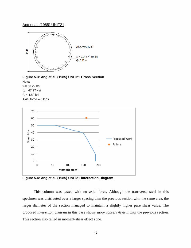
42

Ang et al. (1985) UNIT21

Figure 5.3: Ang et al. (1985) UNIT21 Cross Section Note: fy = 63.22 ksi fyt = 47.27 ksi f’c = 4.82 ksi Axial force = 0 kips

Figure 5.4: Ang et al. (1985) UNIT21 Interaction Diagram

This column was tested with no axial force. Although the transverse steel in this

specimen was distributed over a larger spacing than the previous section with the same area, the

larger diameter of the section managed to maintain a slightly higher pure shear value. The

proposed interaction diagram in this case shows more conservativism than the previous section.

This section also failed in moment-shear effect zone.

0

10

20

30

40

50

60

70

0 50 100 150 200

Shea

r kip

s

Moment kip.ft

Proposed Work

Failure

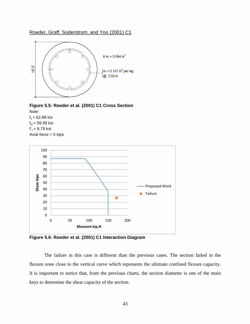
43

Roeder, Graff, Soderstrom, and Yoo (2001) C1

Figure 5.5: Roeder et al. (2001) C1 Cross Section Note: fy = 62.88 ksi fyt = 59.99 ksi f’c = 8.79 ksi Axial force = 0 kips

Figure 5.6: Roeder et al. (2001) C1 Interaction Diagram

The failure in this case is different than the previous cases. The section failed in the

flexure zone close to the vertical curve which represents the ultimate confined flexure capacity.

It is important to notice that, from the previous charts, the section diameter is one of the main

keys to determine the shear capacity of the section.

0

10

20

30

40

50

60

70

80

90

100

0 50 100 150 200

Shea

r kip

s

Moment kip.ft

Proposed Work

Failure

44

Ranf, Eberhard, and Stanton (2006) SpecimenC2

Figure 5.7: Ranf et al. (2006) SpecimenC2 Cross Section Note: fy = 62.98 ksi fyt = 60.03 ksi f’c = 8.27 ksi Axial force = 259.57 kips

Figure 5.8: Ranf et al. (2006) SpecimenC2 Interaction Diagram

This section was tested under a constant axial force of 259.57 kips. This section has

smaller transverse steel area and a larger spacing than the previous section, yet it managed to

reach a slightly larger value due to the presence of the constant axial force and the larger

diameter. From this chart it is important to establish a relationship between the shear force value

and the axial force. The proposed interaction diagram was fairly accurate and conservative

against the failure point.

0102030405060708090

100

0 100 200 300 400

Shea

r kip

s

Moment kip.ft

Proposed Work

Failure

45

Zahn, Park, and Priestley (1986) No.5

Figure 5.9: Zahn et al. (1986) No.5 Cross Section Note: fy = 48.87 ksi fyt = 67.57 ksi f’c = 4.67 ksi Axial force = 124.76 kips

Figure 5.10: Zahn et al. (1986) No.5 Interaction Diagram

A constant axial force of 124.76 kips was applied on this section while testing against

lateral displacement. The failure happened due to flexural effect as the failure point was located

in the flexure zone. The proposed work showed a high accuracy against the failure point.

0

10

20

30

40

50

60

70

80

0 50 100 150 200

Shea

r kip

s

Moment kip.ft

Proposed Work

Failure

46

Pontangaroa, Priestley, and Park (1979) Unit4

Figure 5.11: Pontangaroa et al. (1979) Unit4 Cross Section Note: fy = 43.94 ksi fyt = 61.34 ksi f’c = 4.78 ksi Axial force = 850.87 kips

Figure 5.12: Pontangaroa et al. (1979) Unit4 Interaction Diagram

This section was tested under a relatively high constant axial force of 850.87 kips. A

quick comparison between this section and the previous sections shows at least 135 kips

difference in maximum shear value. This comparison presents the axial force as an important key

to increase the shear capacity of the section.

0

50

100

150

200

250

0 200 400 600 800

Shea

r kip

s

Moment kip.ft

Proposed Work

Failure

47

Nelson (2000) Col4

Figure 5.13: Nelson (2000) Col4 Cross Section Note: fy = 65.98 ksi fyt = 65.98 ksi f’c = 7.65 ksi Axial force = 256.05 kips

Figure 5.14: Nelson (2000) Col4 Interaction Diagram

This section was tested under 256 kips constant axial force. The interaction diagram and

the failure point are similar to Ranf et al. (2006) SpecimenC2 due to the similarity in section

properties and loading conditions. The proposed interaction diagram is accurate and conservative

against the failure point.

0

20

40

60

80

100

120

0 100 200 300 400

Shea

r kip

s

Moment kip.ft

Proposed Work

Failure

48

Lehman and Moehle (2000) No.430

Figure 5.15: Lehman and Moehle (2000) No.430 Cross Section Note: fy = 67 ksi fyt = 88 ksi f’c = 4.5 ksi Axial force = 147 kips

Figure 5.16: Lehman and Moehle (2000) No.430 Interaction Diagram

This section has a relatively high maximum shear value. Although this section was tested

under only 147 kips, comparing to Pontangaroa et al. (1979) Unit4, the shear maximum value is

almost 200 kips (Pontangaroa et al. Unit4 value is 225 kips) due to the smaller spacing and the

higher transverse steel yielding strength.

0

50

100

150

200

250

0 200 400 600 800 1000

Shea

r kip

s

Moment kip.ft

Proposed Work

Failure

49

Kunnath, El-Bahy, Taylor, and Stone (1997) A8

Figure 5.17: Kunnath et al. (1997) A8 Cross Section Note: fy = 64.96 ksi fyt = 62.93 ksi f’c = 4.76 ksi Axial force = 49.91 kips

Figure 5.18: Kunnath et al. (1997) A8 Interaction Diagram

The section was tested under 49.9 kips axial force while exposed to lateral loads. It failed

in the flexural zone of the interaction diagram. The predicted interaction diagram is also

conservative and accurate against the failure point.

0

5

10

15

20

25

30

35

40

45

50

0 20 40 60 80

Shea

r kip

s

Moment kip.ft

Proposed Work

Failure

50

Moyer and Kowalsky (2003) Unit1

Figure 5.19: Moyer and Kowalsky (2003) Unit1 Cross Section Note: fy = 82 ksi fyt = 62.99 ksi f’c = 4.75 ksi Axial force = 52 kips

Figure 5.20: Moyer and Kowalsky (2003) Unit1 Interaction Diagram

0

10

20

30

40

50

60

70

80

90

100

0 100 200 300

Shea

r kip

s

Moment kip.ft

Proposed Work

Failure

51

Siryo (1975) BRI-No.3-ws22bs

Figure 5.21: Siryo (1975) BRI-No.3-ws22bs Cross Section Note: fy = 54.38 ksi fyt = 53.07 ksi f’c = 4.59 ksi Axial force = 72.39 kips

Figure 5.22: Siryo (1975) BRI-No.3-ws22bs Interaction Diagram

0

5

10

15

20

25

30

0 10 20 30 40

Shea

r kip

s

Moment kip.ft

Proposed Work

Failure

52

Henry and Mahin (1999) No.415s

Figure 5.23: Henry and Mahin (1999) No.415s Cross Section Note: fy = 67 ksi fyt = 88 ksi f’c = 5.4 ksi Axial force = 147 kips

Figure 5.24: Henry and Mahin (1999) No.415s Interaction Diagram

This section was tested by Henry and Mahin (1999) under an axial force of 147 kips.

Comparing this section to Lehman and Moehle (2000) No430 section, both sections have the

same cross section diameter, transverse steel area, material properties, and axial load. However,

the Lehman and Moehle section’s maximum shear capacity was 75 kips more than the Henry and

Mahin section’s shear capacity because of the smaller spacing. Fifty percent smaller spacing, in

0

20

40

60

80

100

120

140

0 200 400 600

Shea

r kip

s

Moment kip.ft

Proposed Work

Failure

53

this example, provided around 30% increase in shear capacity. It is clear that spacing is one of

the master keys to provide more shear strength to the section.

Hamilton, Pardoen, and Kazanjy (2002) UC3

Figure 5.25: Hamilton et al. (2002) UC3 Cross Section Note: fy = 66.5 ksi fyt = 100 ksi f’c = 5.17 ksi Axial force = 0 kips

Figure 5.26: Hamilton et al. (2002) UC3 Interaction Diagram

0

10

20

30

40

50

60

0 50 100 150 200

Shea

r kip

s

Moment kip.ft

Proposed Work

Failure

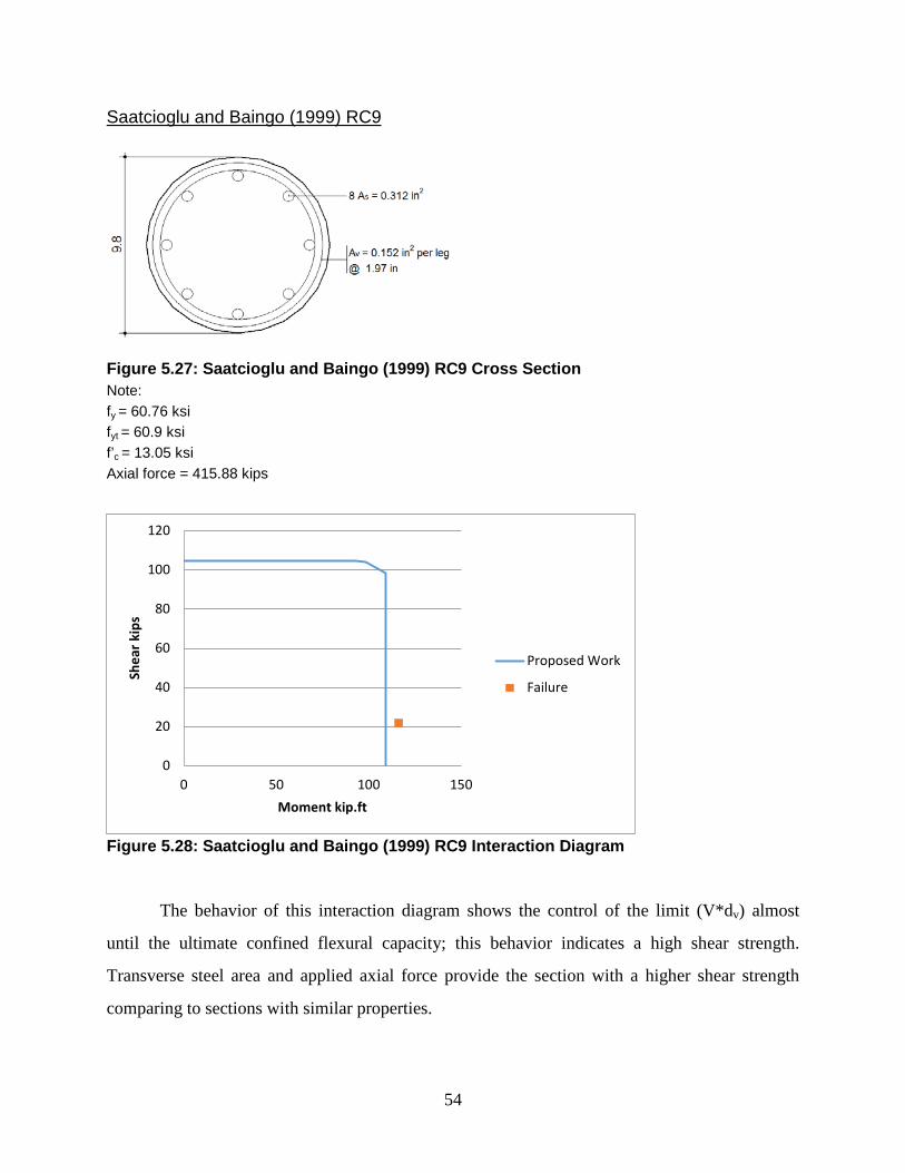
54

Saatcioglu and Baingo (1999) RC9

Figure 5.27: Saatcioglu and Baingo (1999) RC9 Cross Section Note: fy = 60.76 ksi fyt = 60.9 ksi f’c = 13.05 ksi Axial force = 415.88 kips

Figure 5.28: Saatcioglu and Baingo (1999) RC9 Interaction Diagram

The behavior of this interaction diagram shows the control of the limit (V*dv) almost

until the ultimate confined flexural capacity; this behavior indicates a high shear strength.

Transverse steel area and applied axial force provide the section with a higher shear strength

comparing to sections with similar properties.

0

20

40

60

80

100

120

0 50 100 150

Shea

r kip

s

Moment kip.ft

Proposed Work

Failure

55

5.4 Comparisons against Response-2000

Response 2000 is a tool developed by Professor Evan C. Bentz and made available as a

freeware on the Internet. He was a key player in developing the SMCFT. This tool is based on

the MCFT, and it predicts shear strength and moment-shear interaction diagrams at specific

levels of axial loads. In this section, a comparison takes place between the interaction diagrams

generated by Response-2000 for AASHTO (1999) based on the MCFT and the present

formulation based on the equations of AASHTO (2014) using the SMCFT to examine the

similarities and differences in moment-shear interaction diagrams of circular reinforced-concrete

columns. Table 5.1 shows the properties of the selected cross sections examined in this chapter.

Ang et al. (1985) UNIT21

Figure 5.29: Ang et al. (1985) UNIT21 Proposed Interaction Diagram vs. Response 2000

Both predicted interaction diagrams are conservative, and Response 2000 showed a

higher accuracy than the proposed work against the experimental failure point.

0

10

20

30

40

50

60

70

0 50 100 150 200 250

Shea

r kip

s

Moment kip.ft

Proposed Work

Response2000

Failure

56

Roeder et al. (2001) C1

Figure 5.30: Roeder et al. (2001) C1 Proposed Interaction Diagram vs. Response 2000

In this case, the failure point locates between the two interaction diagrams. The proposed

work is more accurate and conservative, while the Response 2000 interaction diagram is less

accurate and less conservative.

Ranf et al. (2006) SpecimenC2

Figure 5.31: Ranf et al. (2006) SpecimenC2 Proposed Interaction Diagram vs. Response 2000

0

20

40

60

80

100

120

0 50 100 150 200

Shea

r kip

s

Moment kip.ft

Proposed Work

Response2000

Failure

0

10

20

30

40

50

60

70

80

90

100

0 100 200 300 400

Shea

r kip

s

Moment kip.ft

Proposed Work

Response2000

Failure

57

Both interaction diagrams are conservative. The proposed interaction diagram shows

more accuracy than Response 2000 against the failure point.

Zahn et al. (1986) No.5

Figure 5.32: Zahn et al. (1986) No.5 Proposed Interaction Diagram vs. Response 2000

Response 2000 interaction diagram is not accurate and not conservative. The proposed

interaction diagram shows a better agreement against the experimental point.

Pontangaroa et al. (1979) Unit4

Figure 5.33: Pontangaroa et al. (1979) Unit4 Proposed Interaction Diagram vs. Response 2000

0

10

20

30

40

50

60

70

80

90

0 50 100 150 200

Shea

r kip

s

Moment kip.ft

Proposed Work

Response2000

Failure

0

50

100

150

200

250

300

0 500 1000 1500

Shea

r kip

s

Moment kip.ft

Proposed Work

Response2000

Failure

58

In this case, the pure moment calculations show a large difference between the two

interaction diagrams. The failure point is located just outside the proposed interaction diagram.

Response 2000 overestimated the moment capacity of the section, causing the failure point to

locate inside its interaction diagram.

Nelson (2000) Col4

Figure 5.34: Nelson (2000) Col4 Proposed Interaction Diagram vs. Response 2000

Both predicted interaction diagrams are conservative. The proposed interaction diagram

accurately estimated the failure envelope of the section, and the failure point locates just outside

the interaction diagram. Response 2000 underestimated the section strength by almost 100 kip.ft.

0

20

40

60

80

100

120

0 100 200 300 400

Shea

r kip

s

Moment kip.ft

Proposed Work

Response2000

Failure

59

Lehman and Moehle (2000) No.430

Figure 5.35: Lehman and Moehle (2000) No.430 Proposed Interaction Diagram vs. Response 2000

In this case, both interaction diagrams were conservative. Response 2000 showed a

slightly better prediction of the failure point than the proposed interaction diagram.

Kunnath et al. (1997) A8

Figure 5.36: Kunnath et al. (1997) A8 Proposed Interaction Diagram vs. Response 2000

Both interaction diagrams were fairly accurate in predicting the failure point.

0

50

100

150

200

250

0 200 400 600 800 1000

Shea

r kip

s

Moment kip.ft

Proposed Work

Response2000

Failure

0

10

20

30

40

50

60

0 20 40 60 80

Shea

r kip

s

Moment kip.ft

Proposed Work

Response2000

Failure

60

Moyer and Kowalsky (2003) Unit1

Figure 5.37: Moyer and Kowalsky (2003) Unit1 Proposed Interaction Diagram vs. Response 2000

The failure point locates between the two interaction diagrams. Response 2000

overestimated section capacity. The proposed interaction diagram managed to accurately predict

the section behavior.

Saatcioglu and Baingo (1999) RC9

Figure 5.38: Saatcioglu and Baingo (1999) RC9 Proposed Interaction Diagram vs. Response 2000

0

20

40

60

80

100

120

140

0 100 200 300 400

Shea

r kip

s

Moment kip.ft

Proposed Work

Response2000

Failure

0

20

40

60

80

100

120

140

0 50 100 150 200

Shea

r kip

s

Moment kip.ft

Proposed Work

Response2000

Failure

61

In this case, Response 2000 failed to estimate the flexural capacity of the section, shifting

the interaction diagram away from the failure point. On the other hand, the proposed interaction

diagram was conservative and accurate in predicting the failure envelope of the section.

In this section, different circular columns and bridge piers were analyzed using the

present AASHTO (2014) formulation to generate the 2D moment-shear interaction diagrams at a

constant axial force. The resulting diagrams are compared against the corresponding

experimental axial force-shear-moment failure point to examine the accuracy of the procedure,

see Table 5.1. In most of the cases, the failure point locates just outside the generated interaction

diagram, indicating that this diagram is accurate and conservative enough. As for some cases like

Hamilton et al. (2002) Unit UC3, it is evident that the experimental points are also outside the

diagrams while the diagrams are more conservative compared to the other specimens that seem

to match the experimental data point very well. It may be concluded from the different

experiments that were dominated by shear failure, bending moment failure, and a combination

thereof that the present AASHTO (2014) procedure examined here for circular bridge piers is

accurate enough when compared to the experiments.

The next step was to examine a head-to-head comparison between the present

formulation and the AASHTO (1999) interaction diagrams developed by the well-known

software Response 2000 using the same assumptions, limits, and overall equations. For this

purpose, ten specimens were selected. Based on the diagrams discussed in this section, it can be

concluded that the present diagrams are more conservative than those of Response 2000 in

moment-dominated failure, indicating that Response 2000 predictions in this region are

erroneous. This is due to the fact that at zero shear force, the moment values indicated by the

present diagrams are the very ultimate values of confined analysis of moment-axial compression

computed by Abd El-Fattah et al. (2011). The fact that Response 2000 moment values exceed

this limit indicates an error in that program’s results. Mapping the experimental data points on

both interaction diagrams supports this finding and indicates the accuracy of the present

formulation over that of Response 2000.

62

5.5 Database

This section provides a tabulated database of the cross sections used to analyze, compare,

and predict the proposed interaction diagram procedure. Chapter 7 provides full results of this

database, based on the proposed calculation in the same order shown in the tables. The

parameters presented in the tables are the parameters needed to predict the interaction diagram

based on the proposed procedures.

63

Table 5.3: Arakawa et al. (1987) Sections

Unit D (in.) Clear cover (in.)

La/D Number of bars

Longitudinal bar diameter

(in.) fy (ksi)

Transverse bar diameter

(in.) fyt (ksi) Spacing

(in.) f'c

(ksi) Axial force (kip)

Shear force (kip)

Moment (k.ft)

UNIT1 10.83 0.67 1.1 12 0.63 53.07 0.24 53.36 3.94 4.18 0 39.65 39.37 UNIT2 10.83 0.67 1.1 12 0.63 53.07 0.24 53.36 1.97 4.25 0 45.82 45.49 UNIT4 10.83 0.67 1.1 12 0.63 53.07 0.24 53.36 3.94 4.33 48.33 44.01 43.7 UNIT6 10.83 0.67 1.1 12 0.63 53.07 0.24 53.36 1.97 4.15 48.33 50.65 50.29 UNIT8 10.83 0.67 1.1 12 0.63 53.07 0.24 53.36 1.38 4.56 48.33 48.53 48.18 UNIT9 10.83 0.67 1.1 16 0.63 53.07 0.24 53.36 1.97 4.43 48.33 51.26 50.89 UNIT10 10.83 0.67 1.1 8 0.63 53.07 0.24 53.36 1.97 4.38 48.33 57.15 56.74 UNIT12 10.83 0.67 1.1 12 0.63 53.07 0.24 53.36 3.94 4.04 96.66 43.15 42.84 UNIT13 10.83 0.67 1.1 12 0.63 53.07 0.24 53.36 1.97 4.43 96.66 53.6 53.22 UNIT14 10.83 0.67 1.1 12 0.63 53.07 0.24 53.36 1.38 4.54 96.66 62.74 62.29 UNIT15 10.83 0.67 1.64 12 0.63 52.64 0.24 55.25 2.95 4.64 0 40.38 59.77 UNIT16 10.83 0.67 1.64 12 0.63 52.64 0.24 55.25 1.38 4.54 0 39.77 58.87 UNIT17 10.83 0.67 1.1 12 0.63 52.64 0.24 55.25 2.95 4.54 48.33 55.43 55.03 UNIT19 10.83 0.67 1.64 12 0.63 52.64 0.24 55.25 2.95 4.53 48.33 41.92 62.05 UNIT20 10.83 0.67 1.64 12 0.63 52.64 0.24 55.25 1.38 4.25 48.33 47.71 70.62 UNIT21 10.83 0.67 2.19 12 0.63 52.64 0.24 55.25 2.95 4.43 48.33 34.67 68.53 UNIT23 15.75 0.43 2 12 0.63 63.22 0.47 48.14 6.3 4.69 48.33 47.7 125.22 UNIT24 10.83 0.67 1.1 12 0.63 52.64 0.24 55.25 2.95 4.51 96.66 52.61 52.23 UNIT25 10.83 0.67 1.64 12 0.63 52.64 0.24 55.25 2.95 4.31 96.66 45.24 66.96 UNIT26 10.83 0.67 2.19 12 0.63 52.64 0.24 55.25 2.95 4.49 96.66 39.15 77.38 UNIT27 10.83 0.67 1.64 12 0.63 52.64 0.24 55.25 2.95 2.75 96.66 39.58 58.59 UNIT28 10.83 0.67 1.64 12 0.63 52.64 0.24 55.25 2.95 5.99 96.66 51.88 76.79

64

Table 5.4: Calderone, Lehman, and Moehle (2001) Sections

Unit D (in.) Clear cover (in.)

La/D Number of bars

Longitudinal bar diameter

(in.) fy (ksi)

Transverse bar diameter

(in.) fyt (ksi) Spacing

(in.) f'c

(ksi) Axial force (kip)

Shear force (kip)

Moment (k.ft)

No.328 24 1 3 28 0.75 63.99 0.25 87.99 1 5.01 204.98 124.76 748.56 No.828 24 1 8 28 0.75 63.99 0.25 87.99 1 5.01 204.98 45.63 730.08 No.1028 24 1 10 28 0.75 63.99 0.25 87.99 1 5.01 204.98 42.8 856

Table 5.5: Henry and Mahin (1999) Sections

Unit D (in.) Clear cover (in.)

La/D Number of bars

Longitudinal bar diameter

(in.) fy (ksi)

Transverse bar diameter

(in.) fyt (ksi) Spacing

(in.) f'c

(ksi) Axial force (kip)

Shear force (kip)

Moment (k.ft)

No.415p 24 0.75 4 22 0.63 66.99 0.25 87.99 1.25 5.4 294.04 74.19 593.52 No.415s 24 0.75 4 22 0.63 66.99 0.25 87.99 2.5 5.4 147.02 64.8 518.4

Table 5.6: Hamilton et al. (2002) Sections

Unit D (in.) Clear cover (in.)

La/D Number of bars

Longitudinal bar diameter (in.) fy (ksi) Transverse bar

diameter (in.) fyt (ksi) Spacing (in.)

f'c (ksi)

Axial force (kip)

Shear force (kip)

Moment (k.ft)

UC13 16 0.32 2.58 14 0.5 66.49 0.18 100.27 6.75 5.04 0 32.21 110.81 UC14 16 0.32 2.58 14 0.5 66.49 0.18 100.27 6.75 5.04 0 36.96 127.15 UC15 16 0.32 2.58 12 0.5 66.49 0.18 100.27 2.5 5.14 0 39.24 134.99 UC1 16 0.5 4.57 12 0.5 66.49 0.18 100.27 1.25 5.3 0 15.81 96.34 UC2 16 0.5 4.57 12 0.5 66.49 0.18 100.27 1.25 5.3 0 16.96 103.35 UC3 16 0.5 4.57 12 0.5 66.49 0.18 100.27 1.25 5.17 0 23.83 145.21

65

Table 5.7: Cheok and Stone (1986) Sections

Unit D (in.) Clear cover (in.)

La/D Number of bars

Longitudinal bar diameter

(in.) fy (ksi)

Transverse bar diameter

(in.) fyt (ksi) Spacing

(in.) f'c

(ksi) Axial force (kip)

Shear force (kip)

Moment (k.ft)

NIST-Full- scale Flexure 59.84 2 6.02 25 1.69 68.88 0.63 71.49 3.5 5.2 1000.36 290.76 8728.54

NIST-Full- scale-shear 59.84 1.75 3.01 25 1.69 68.88 0.75 63.08 2.13 4.98 1000.36 737.79 11074.13

Table 5.8: Chai, Priestley, and Seible (1991) Sections

Unit D (in.) Clear cover (in.)

La/D Number of bars

Longitudinal bar diameter

(in.) fy (ksi)

Transverse bar diameter

(in.) fyt (ksi) Spacing

(in.) f'c

(ksi) Axial force (kip)

Shear force (kip)

Moment (k.ft)

CCS1 24.02 0.55 2 26 0.75 45.71 0.25 46.13 5 5.01 135.96 124.2 497.22 Test3 24 0.66 6 26 0.75 45.69 0.25 50.99 5 4.73 399.92 55.74 668.88 UNIT1 24 0.55 6 26 0.75 45.7 0.25 51 5 5.54 400 48.5 582

Table 5.9: Siryo (1975) Sections

Unit D (in.) Clear cover (in.)

La/D Number of bars

Longitudinal bar diameter

(in.) fy (ksi)

Transverse bar diameter

(in.) fyt (ksi) Spacing

(in.) f'c

(ksi) Axial force (kip)

Shear force (kip)

Moment (k.ft)

BRI-No.2 9.84 1.4 1.5 4 0.38 57.86 0.35 51.48 1.97 3.85 41.36 27.96 34.4 BRI-No.3- ws22bs 9.84 1.38 2.01 8 0.37 54.38 0.23 53.07 2.48 4.59 72.39 23.08 38.05

BRI-No.3- ws27bs 9.84 1.4 2.01 8 0.63 50.03 0.35 48.51 1.65 4.59 72.39 33.25 54.81

ws21bs 9.84 1.4 1 8 0.37 54.38 0.35 48.51 1.3 3.85 72.39 41.32 33.89 ws25bs 9.84 1.34 1 8 0.5 55.39 0.35 48.51 1.81 3.85 36.19 41.59 34.11 ws26bs 9.84 1.38 2.01 8 0.5 55.39 0.15 56.05 1.46 4.59 36.19 23.52 38.77

66

Table 5.10: Kowalesky and Priestley (2000) Sections

Unit D (in.) Clear cover (in.)

La/D Number of bars

Longitudinal bar diameter (in.) fy (ksi) Transverse bar

diameter (in.) fyt (ksi) Spacing (in.)

f'c (ksi)

Axial force (kip)

Shear force (kip)

Moment (k.ft)

FL1 17.99 1 8.01 30 0.63 69.17 0.37 64.53 2.99 5.31 400.14 42.04 504.83 FL2 17.99 1.06 8.01 30 0.63 69.17 0.25 63.37 2.01 5.8 400.14 39.28 471.69 FL3 17.99 1.06 8.01 30 0.63 69.17 0.25 64.53 2.99 5.6 400.14 44.38 532.93

Table 5.11: Hose, Seible, and Priestley (1997) Section and Elsanadedy (2002) Section

Unit D (in.) Clear cover (in.)

La/D Number of bars

Longitudinal bar diameter

(in.) fy (ksi)

Transverse bar diameter

(in.) fyt (ksi) Spacing

(in.) f'c

(ksi) Axial force (kip)

Shear force (kip)

Moment (k.ft)

SRPH1 24.02 0.91 6 20 0.87 65.98 0.37 60.03 2.24 5.96 400.14 81.75 981.82 UnitCS-A1 24 0.75 2 20 0.75 43.41 0.25 30.51 5 5.35 145 102.1 408.4

Table 5.12: Moyer and Kowalsky (2003) Sections

Unit D (in.) Clear cover (in.)

La/D Number of bars

Longitudinal bar diameter (in.) fy (ksi) Transverse bar

diameter (in.) fyt (ksi) Spacing (in.)

f'c (ksi)

Axial force (kip)

Shear force (kip)

Moment (k.ft)

Unit_1 18 0.31 5.34 12 0.75 81.99 0.37 62.99 3 4.75 52 34.86 279.23 Unit_2 18 0.31 5.34 12 0.75 81.99 0.37 62.99 3 4.96 52 35.8 286.76 Unit_3 18 0.31 5.34 12 0.75 81.99 0.37 62.99 3 4.6 52 43.08 345.08 Unit_4 18 0.31 5.34 12 0.75 81.99 0.37 62.99 3 4.92 52 35.32 282.92

67

Table 5.13: Ng, Lam, and Kwan (2010) Sections

Unit D (in.)

Clear cover (in.)

La/D Number of bars

Longitudinal bar diameter (in.) fy (ksi) Transverse bar

diameter (in.) fyt (ksi) Spacing (in.)

f'c (ksi)

Axial force (kip)

Shear force (kip)

Moment (k.ft)

No.2 9.84 0.34 5.37 10 0.51 44.23 0.17 38.14 0.55 5.09 3.8 8.23 36.24 No.3 9.84 0.32 3.73 10 0.47 42.63 0.17 30.02 0.39 4.79 123.64 17.56 53.71

Table 5.14: Kunnath et al. (1997) Sections

Unit D (in.) Clear cover (in.)

La/D Number of bars

Longitudinal bar diameter (in.) fy (ksi) Transverse bar

diameter (in.) fyt (ksi) Spacing (in.)

f'c (ksi)

Axial force (kip)

Shear force (kip)

Moment (k.ft)

A2 12.01 0.49 4.5 21 0.37 64.96 0.16 62.93 0.75 4.21 44.96 16.63 74.9 A3 12.01 0.49 4.5 21 0.37 64.96 0.16 62.93 0.75 4.21 44.96 16.93 76.25 A4 12.01 0.49 4.5 21 0.37 64.96 0.16 62.93 0.75 5.15 49.91 16.97 76.43 A5 12.01 0.49 4.5 21 0.37 64.96 0.16 62.93 0.75 5.15 49.91 20.86 93.95 A6 12.01 0.49 4.5 21 0.37 64.96 0.16 62.93 0.75 5.15 49.91 17.26 77.74 A7 12.01 0.49 4.5 21 0.37 64.96 0.16 62.93 0.75 4.76 49.91 17.75 79.95 A8 12.01 0.49 4.5 21 0.37 64.96 0.16 62.93 0.75 4.76 49.91 16.42 73.96 A9 12.01 0.49 4.5 21 0.37 64.96 0.16 62.93 0.75 4.72 49.91 16.86 75.94 A10 12.01 0.49 4.5 21 0.37 64.96 0.16 62.93 0.75 3.92 44.96 16.69 75.17 A11 12.01 0.49 4.5 21 0.37 64.96 0.16 62.93 0.75 3.92 44.96 16.3 73.42 A12 12.01 0.49 4.5 21 0.37 64.96 0.16 62.93 0.75 3.92 44.96 16.25 73.19

68

Table 5.15: Lehman and Moehle (2000) Sections

Unit D (in.) Clear cover (in.)

La/D Number of bars

Longitudinal bar diameter

(in.) fy (ksi)

Transverse bar diameter

(in.) fyt (ksi) Spacing

(in.) f'c

(ksi) Axial force (kip)

Shear force (kip)

Moment (k.ft)

No.415 24 0.75 4 22 0.63 66.99 0.25 87.99 1.25 4.5 146.99 64.07 512.56 No.815 24 0.75 8 22 0.63 66.99 0.25 87.99 1.25 4.5 146.99 33.94 543.04 No.1015 24 0.75 10 22 0.63 66.99 0.25 87.99 1.25 4.5 146.99 22.82 456.4 No.407 24 0.75 4 11 0.63 66.99 0.25 87.99 1.25 4.5 146.99 40.46 323.68 No.430 24 0.75 4 44 0.63 66.99 0.25 87.99 1.25 4.5 146.99 107.9 863.2

Table 5.16: Lim and McLean (1991) Sections

Unit D (in.)

Clear cover (in.)

La/D Number of bars

Longitudinal bar diameter (in.) fy (ksi) Transverse bar

diameter (in.) fyt (ksi) Spacing (in.)

f'c (ksi)

Axial force (kip)

Shear force (kip)

Moment (k.ft)

Con1 5.98 0.33 7.51 8 0.5 64.96 0.15 89.9 0.87 5.01 33.94 4.28 16.02 Con2 5.98 0.33 3.76 8 0.5 64.96 0.15 89.9 0.87 5.01 33.94 9.3 17.43 Con3 5.98 0.33 3.76 8 0.5 64.96 0.15 89.9 0.87 5.01 49.46 9.67 18.12

Table 5.17: Munro, Park, and Priestley (1976) Section and Iwasaki et al. (1986) Section

Unit D (in.) Clear cover (in.)

La/D Number of bars

Longitudinal bar diameter (in.) fy (ksi) Transverse bar

diameter (in.) fyt (ksi) Spacing (in.)

f'c (ksi)

Axial force (kip)

Shear force (kip)

Moment (k.ft)

No.1 19.69 0.64 5.46 20 0.72 44.23 0.31 56.41 1.34 5.8 5.93 31.1 278.63 I30 22.2 1.38 1.78 40 0.51 46.84 0.35 37.47 8.9 5.77 0 91.37 300.89

69

Table 5.18: McDaniel (1997) Sections

Unit D (in.) Clear cover (in.)

La/D Number of bars

Longitudinal bar diameter

(in.) fy (ksi)

Transverse bar diameter

(in.) fyt (ksi) Spacing

(in.) f'c

(ksi) Axial force (kip)

Shear force (kip)

Moment (k.ft)

UNITS-1 24 0.64 2 20 0.63 65.83 0.19 29 4 4.33 4.23 91.15 364.6 UNITS1-2 24 0.64 2 20 0.63 65.83 0.19 29 4 3.89 4.23 74.7 298.8 UNITS2 24 0.64 2 20 0.63 63.46 0.19 29 4 4.53 4.23 74.7 298.8

Table 5.19: Jaradat (1996) Sections

Unit D (in.) Clear cover (in.)

La/D Number of bars

Longitudinal bar diameter

(in.) fy (ksi)

Transverse bar diameter

(in.) fyt (ksi) Spacing

(in.) f'c

(ksi) Axial force (kip)

Shear force (kip)

Moment (k.ft)

SpecimenS1 10 1.44 2 8 0.5 53.81 0.15 30.51 3.85 4.21 19 17.84 29.74 SpecimenS3 10 1.56 2 8 0.38 52.11 0.15 30.51 3.85 3.81 17 17.34 28.9

Table 5.20: Nelson (2000) Sections

Unit D (in.) Clear cover (in.)

La/D Number of bars

Longitudinal bar diameter

(in.) fy (ksi)

Transverse bar diameter

(in.) fyt (ksi) Spacing

(in.) f'c

(ksi) Axial force (kip)

Shear force (kip)

Moment (k.ft)

Col1 20 0.75 3 10 0.63 65.98 0.18 65.98 4.02 8.15 325.96 69.32 346.6 Col2 20 0.75 3 10 0.63 65.98 0.18 65.98 4.02 8.17 279.43 65.95 329.75 Col3 20 0.75 3 10 0.63 65.98 0.18 65.98 4.02 8.27 256.05 61.89 309.45 Col4 20 0.75 3 10 0.63 65.98 0.18 65.98 4.02 7.65 256.05 59.64 298.2

70

Table 5.21: Priestley et al. (1994) Sections

Unit D (in.) Clear cover (in.)

La/D Number of bars

Longitudinal bar diameter (in.) fy (ksi) Transverse bar

diameter (in.) fyt (ksi) Spacing (in.)

f'c (ksi)

Axial force (kip)

Shear force (kip)

Moment (k.ft)

NR1 24.02 0.5 1.5 12 0.5 66.99 0.25 52.35 3 4.35 113.07 94.05 282.39 NR2 24.02 0.5 1.5 24 0.5 66.99 0.25 52.35 5 4.35 113.07 132.04 396.46

Table 5.22: Petrovski and Ristic (1984) Sections

Unit D (in.) Clear cover (in.)

La/D Number of bars

Longitudinal bar diameter (in.) fy (ksi) Transverse bar

diameter (in.) fyt (ksi) Spacing (in.)

f'c (ksi)

Axial force (kip)

Shear force (kip)

Moment (k.ft)

M1E1 12.09 1.3 6.23 12 0.47 34.8 0.24 34.8 2.95 5.63 32.6 7.55 47.39 M1E2 12.09 1.3 6.23 12 0.47 34.8 0.24 34.8 2.95 5.25 57.1 8.31 52.16 M2E1 12.09 1.3 2.94 12 0.47 34.8 0.24 34.8 1.42 5.21 32.6 19.32 57.23 M2E2 12.09 1.3 2.92 12 0.47 34.8 0.24 34.8 1.42 4.99 57.1 20.9 61.49

Table 5.23: Zahn et al. (1986) Sections

Unit D (in.) Clear cover (in.)

La/D Number of bars

Longitudinal bar diameter (in.) fy (ksi) Transverse bar

diameter (in.) fyt (ksi) Spacing (in.)

f'c (ksi)

Axial force (kip)

Shear force (kip)

Moment (k.ft)

No.5 15.75 0.51 4 16 0.63 48.87 0.39 67.57 5.31 4.67 124.76 32 168 No.6 15.75 0.51 4 16 0.63 48.87 0.39 67.57 2.95 3.92 467.58 39.37 206.7

71

Table 5.24: Pontangaroa et al. (1979) Sections

Unit D (in.) Clear cover (in.)

La/D Number of bars

Longitudinal bar diameter

(in.) fy (ksi)

Transverse bar diameter

(in.) fyt (ksi) Spacing

(in.) f'c

(ksi) Axial force (kip)

Shear force (kip)

Moment (k.ft)

Unit1 23.62 0.79 2 16 0.94 43.94 0.39 43.5 2.95 4.12 431.62 154.47 608.1 Unit4 23.62 0.79 2 16 0.94 43.94 0.39 61.34 2.76 4.78 850.87 175.54 691.05 No.5A 23.62 0.79 2 16 0.94 44.52 0.63 40.6 2.17 4.72 760.95 182.48 718.37 No.5B 23.62 0.79 2 16 0.94 44.52 0.63 40.6 2.17 4.72 1521.9 210.65 829.26

Table 5.25: Watson and Park (1994) Sections

Unit D (in.) Clear cover (in.)

La/D Number of bars

Longitudinal bar diameter

(in.) fy (ksi)

Transverse bar diameter

(in.) fyt (ksi) Spacing

(in.) f'c

(ksi) Axial force (kip)

Shear force (kip)

Moment (k.ft)

No.10 15.75 0.51 4 12 0.63 68.73 0.31 53.94 3.31 5.8 596.17 47.72 250.53 No.11 15.75 0.51 4 12 0.63 68.73 0.39 49.01 2.24 5.66 813.78 46.41 243.66

Table 5.26: Ranf et al. (2006) Sections

Unit D (in.) Clear cover (in.)

La/D Number of bars

Longitudinal bar diameter

(in.) fy (ksi)

Transverse bar diameter

(in.) fyt (ksi) Spacing

(in.) f'c

(ksi) Axial force (kip)

Shear force (kip)

Moment (k.ft)

SpecimenS1 20 0.57 3 10 0.62 65.98 0.18 60.03 4 5.28 165.62 48.31 241.55 SpecimenC2 20 0.57 3 10 0.62 65.98 0.18 60.03 4 8.27 259.57 62.06 310.3 SpecimenC3R 20 0.57 3 10 0.62 65.98 0.18 60.03 4 7.65 240.07 59.99 299.95 SpecimenS3 20 0.57 3 10 0.62 65.98 0.18 60.03 4 8.16 256.11 59.87 299.35

72

Table 5.27: Yalcin (1997) Section and Yarandi (2007) Section

Unit D (in.) Clear cover (in.)

La/D Number of bars

Longitudinal bar diameter

(in.) fy (ksi)

Transverse bar diameter

(in.) fyt (ksi) Spacing

(in.) f'c

(ksi) Axial force (kip)

Shear force (kip)

Moment (k.ft)

SpecimenBR-C1 24.02 2.17 2.44 12 0.98 64.53 0.39 61.63 11.81 6.53 404.46 126.45 617.6 SpecimenCR-C 23.62 1.77 2.5 12 0.77 67.43 0.25 71.2 11.81 5.08 311.43 95.23 468.62

Table 5.28: Roeder et al. (2001) Sections

Unit D (in.) Clear cover (in.)

La/D Number of bars

Longitudinal bar diameter

(in.) fy (ksi)

Transverse bar diameter

(in.) fyt (ksi) Spacing

(in.) f'c

(ksi) Axial force (kip)

Shear force (kip)

Moment (k.ft)

C1 16.5 2 4.7 8 0.87 62.28 0.37 59.99 2 8.79 0 26.59 171.84 C2 16.5 2 4.7 8 0.87 62.28 0.37 59.99 2 9.08 0 27.21 175.85 C3 16.5 2 4.7 8 0.87 62.28 0.39 59.99 2 10.1 0 30.69 198.34 C4 16.5 2 4.7 8 0.87 62.28 0.39 59.99 2 10.1 221.99 38.28 247.39 C5 16.5 2 4.7 8 0.87 71.29 0.39 59.99 2 10.1 221.99 41.29 266.84 C6 16.5 2 4.7 8 0.87 73.37 0.39 59.99 2 10.1 221.99 40.83 263.87 C7 16.5 2 4.7 8 0.87 73.37 0.39 59.99 2 10.1 221.99 39.92 257.99 C8 16.5 2 4.7 8 0.87 71.29 0.39 59.99 2 10.1 221.99 44.59 288.17

Table 5.29: Sritharan, Priestley, and Seible (2001) Sections

Unit D (in.) Clear cover (in.)

La/D Number of bars

Longitudinal bar diameter

(in.) fy (ksi)

Transverse bar diameter

(in.) fyt (ksi) Spacing

(in.) f'c

(ksi) Axial force (kip)

Shear force (kip)

Moment (k.ft)

IC1 23.62 1 3.01 14 0.87 64.96 0.37 62.5 3.82 4.56 89.92 97.48 577.54 B105IC2 23.62 1 3.01 14 0.87 64.96 0.37 62.5 3.82 5.02 89.92 96.79 573.46 IC3 23.62 1 3.01 14 0.87 62.93 0.37 62.93 2.52 4.79 89.92 103.48 613.09

73

Table 5.30: Stone and Cheok (1989) Sections

Unit D (in.) Clear cover (in.)

La/D Number of bars

Longitudinal bar diameter

(in.) fy (ksi)

Transverse bar diameter

(in.) fyt (ksi) Spacing

(in.) f'c

(ksi) Axial force (kip)

Shear force (kip)

Moment (k.ft)

NIST-Model-N1 9.84 0.33 3.01 25 0.28 64.67 0.12 63.95 0.35 3.5 26.98 14.41 35.57 NIST-Model-N2 9.84 0.33 3.01 25 0.28 64.67 0.12 63.95 0.35 3.35 53.73 16.51 40.75 NIST-Model-N3 9.84 0.33 6.01 25 0.28 64.67 0.11 69.02 0.55 3.69 26.98 7.17 35.34 NIST-Model-N4 9.84 0.33 3.01 25 0.28 64.67 0.12 63.95 0.35 3.54 26.98 14.1 34.81 NIST-Model-N5 9.84 0.33 3.01 25 0.28 64.67 0.12 63.95 0.35 3.53 53.73 17.21 42.48 NIST-Model-N6 9.84 0.33 6.01 25 0.28 64.67 0.11 63.95 0.55 3.38 26.98 6.67 32.88

Table 5.31: Vu, Priestley, Seible, and Benzoni (1998) Sections

Unit D (in.) Clear cover (in.)

La/D Number of bars

Longitudinal bar diameter (in.) fy (ksi) Transverse bar

diameter (in.) fyt (ksi) Spacing (in.)

f'c (ksi)

Axial force (kip)

Shear force (kip)

Moment (k.ft)

NH1 18 0.79 2 20 0.63 62 0.37 62.38 2.36 5.56 433.41 139.38 417.91 NH3 18 0.79 2 20 0.63 62 0.37 62.38 2.36 5.72 218.06 124 371.8 NH4 18 0.79 2 30 0.75 67.89 0.5 63 1.77 5.08 191.08 221.45 663.99 NH6 18 0.79 2 30 0.75 70.5 0.5 63 1.57 5.08 430.27 249.3 747.49

Table 5.32: Wong (1990) Sections

Unit D (in.) Clear cover (in.)

La/D Number of bars

Longitudinal bar diameter

(in.) fy (ksi)

Transverse bar diameter

(in.) fyt (ksi) Spacing

(in.) f'c

(ksi) Axial force (kip)

Shear force (kip)

Moment (k.ft)

UnitNo.2 15.75 0.59 2 20 0.63 68.88 0.24 49.3 2.56 5.37 411.38 109.99 288.73 UnitNo.1 15.75 0.59 2 20 0.63 61.34 0.39 43.5 2.36 5.51 203.89 103.69 272.19 UnitNo.3 15.75 0.59 2 20 0.63 68.88 0.39 43.5 2.36 5.37 407.56 130.07 341.44

74

Table 5.33: Ang et al. (1985) Sections

Unit D (in.) Clear cover (in.)

La/D Number of bars

Longitudinal bar diameter (in.) fy (ksi) Tranverse bar

diameter (in.) fyt (ksi) Spacing (in.)

f'c (ksi)

Axial force (kip)

Shear force (kip)

Moment (k.ft)

1 15.75 0.59 2 20 0.63 63.22 0.24 47.56 2.36 5.44 0 72.25 189.66 2 15.75 0.59 2 20 0.63 42.92 0.24 47.56 2.36 5.4 0 49.61 130.23 3 15.75 0.59 2.5 20 0.63 63.22 0.24 47.56 2.36 5.22 0 62.09 203.71 4 15.75 0.59 2 20 0.63 63.22 0.39 45.82 6.5 4.44 0 65.01 170.66 5 15.75 0.59 2 20 0.63 63.22 0.24 47.56 1.57 4.51 0 74.39 195.28 6 15.75 0.59 1.5 20 0.63 63.22 0.24 47.56 2.36 4.37 0 88.04 173.3 7 15.75 0.59 2 20 0.63 64.96 0.24 53.94 3.15 4.28 0 63.09 165.62 8 15.75 0.59 2 20 0.63 64.96 0.24 53.94 1.18 4.17 162.08 104.54 274.42 9 15.75 0.59 2.5 20 0.63 64.96 0.24 53.94 1.18 4.53 0 101.037 266.15 10 15.75 0.59 2 20 0.63 64.96 0.47 48.14 4.72 4.34 176.24 101.39 240.24 11 15.75 0.59 2 20 0.63 64.96 0.24 53.94 2.36 4.15 168.82 91.52 233.13 12 15.75 0.59 1.5 20 0.63 64.96 0.24 53.94 1.17 5.25 80.7 118.44 259.85 13 15.75 0.59 2 20 0.63 63.22 0.24 47.27 1.18 4.89 102.28 98.99 186.69 14 15.75 0.43 2 9 0.94 61.48 0.24 47.27 2.36 5.05 0 71.12 135.93 15 15.75 0.59 2 12 0.63 63.22 0.24 47.27 2.36 4.85 0 51.78 219.66 16 15.75 0.59 2 20 0.63 63.22 0.24 47.27 2.36 4.98 94.42 83.68 239.9 17 15.75 0.59 2.5 20 0.63 63.22 0.24 47.27 2.36 5.08 96.89 73.12 297.92 18 15.75 0.59 2 20 0.63 63.22 0.24 47.27 2.36 4.99 98.91 113.49 193.57 19 15.75 0.59 1.5 20 0.63 63.22 0.24 47.27 3.15 5.33 97.11 98.34 251.26 20 15.75 0.59 1.75 20 0.63 69.89 0.24 47.27 3.15 4.82 181.41 109.4 159.6 21 15.75 0.59 2 20 0.63 63.22 0.24 47.27 3.15 4.49 0 60.8 168.08 22 15.75 0.59 2 20 0.63 63.22 0.39 44.95 8.66 4.69 0 64.03 196.22 23 15.75 0.59 2 20 0.63 63.22 0.47 48.14 6.3 4.8 0 74.75 200.92 24 15.75 0.59 2 20 0.63 63.22 0.39 44.95 4.33 0 0 76.54 0

75

Chapter 6: Software Development

6.1 Introduction

The proposed procedure was built into the KDOT Column Expert software in order to

compute the full domain moment-shear-axial force interaction diagram for circular reinforced-

concrete column sections (Rasheed, Abd El-Fattah, Esmaeily, Jones, & Hurst, 2012). KDOT

Column Expert is an object oriented program written within the framework of the visual C#

language. This software can predict the steel confined and unconfined moment-axial force

capacity for circular and rectangular sections. By adding shear analysis to the software, KDOT

Column Expert can predict the full domain of the sections under the three major loads: moment-

axial-shear force combinations. In this chapter, input interface and output interface are discussed

for circular sections for the cases where shear is a key design of the load combinations.

6.2 Input Interface

The input data is divided into four subsections. The geometrical properties are the first

subsection, including section diameter, clear cover, number of bars, number of longitudinal and

transverse bars, and spacing. The second subsection is the concrete properties, including the

concrete compressive strength and its corresponding strain, as well as the maximum strain. The

third and fourth subsections are for the longitudinal and transverse steel properties. Steel

properties are Young’s modulus and yielding strength of the steel. The user also has the option to

choose the transverse steel order between the two main orders, spiral and hoops. Figure 6.1

shows the input properties interface of the section.

76

Figure 6.1: KDOT Column Expert Input Interface

The custom check box beside the steel bar textbox is to give the user the option to define

the steel bar diameter if the bar diameter is not within the US rebar size charts, see Figure 6.2.

Figure 6.2: KDOT Column Expert Custom Bars Input

77

6.3 Output Interface

The default output interaction diagram is the moment versus axial force with zero shear

value, see Figure 6.1. It shows the steel confined (red curve) and unconfined (green curve)

section capacities.

In order to account for the shear calculations, the “Plot Shear-Moment” button was

added. This button generates the interaction diagram for moment and shear force at a constant

axial force defined by the user, see Figure 6.3. Figure 6.4 shows the final output of the “Plot

Shear-Moment” button for constant axial force. The full domain could be generated using the

“Interaction Domain” button, where the calculation in “Plot Shear-Moment” is repeated for a

series of axial forces up to the maximum confined axial load capacity. Figure 6.5 shows the full

domain of moment-axial force-shear force combination.

Figure 6.3: KDOT Column Expert Axial Force Input

78

Figure 6.4: KDOT Column Expert 2D Moment-Shear Interaction Diagram

Figure 6.5: KDOT Column Expert 3D Domain

79

In the case of sections having transverse steel less than the minimum transverse steel

defined by AASHTO (2014) LRFD Bridge Construction Specifications, the user is asked to

provide a value of maximum aggregate size; see Figures 6.6 and 6.7.

Figure 6.6: Minimum Transverse Steel

Figure 6.7: Maximum Aggregate Size Input

There are three cases in which AASHTO (2014) LRFD Specifications consider the

section invalid, and will ask to change the properties of the section. In KDOT Column Expert,

the user is notified to change the section properties if any of these cases matched. The first case

occurs if the transverse steel spacing exceeded the maximum; in this case the message shown in

Figure 6.8 appears and the analysis stops.

Figure 6.8: Maximum Spacing Error Message

80

The second case is to make sure that the section has enough longitudinal steel to resist

cracks in the case of sections having transverse steel less than the minimum transverse steel

defined by AASHTO (2014) LRFD Specifications. Figure 6.9 shows the KDOT Column Expert

message to the user in this case.

Figure 6.9: Lack of Longitudinal Steel Error

The third case is to confirm that the transverse steel yielding strength is less than 100 ksi.

This limit is established to have a clear yielding zone in the steel stress-strain curve. If the

transverse steel yielding strength exceeded 100 ksi, the yielding zone vanishes. Figure 6.10

shows the KDOT Column Expert message to the user in this case.

Figure 6.10: Transverse Steel Exceeded 100 ksi Error

81

Chapter 7: Complete Database Comparisons of AASHTO LRFD Approach

This chapter provides the interaction diagrams for the full database discussed in Chapter

5 based on the AASHTO (2014) LRFD Bridge Construction Specifications approach. In this

chapter, the calculated interaction diagram is represented as a solid line, while the reported

experimental failure point is represented as a square mark.

Figure 7.1: Arakawa et al. (1987) Interaction Diagrams (UNITs 1, 2, 4, and 6; Table 5.3)

05

1015202530354045

0 20 40 60 80

Shea

r kip

s

Moment kip.ft

0

10

20

30

40

50

0 20 40 60 80

Shea

r kip

s

Moment kip.ft

0

10

20

30

40

50

0 20 40 60 80

Shea

r kip

s

Moment kip.ft

0

10

20

30

40

50

60

0 20 40 60 80

Shea

r kip

s

Moment kip.ft

82

Figure 7.2: Arakawa et al. (1987) Interaction Diagrams (UNITs 8, 9, 10, 12, 13, and 14; Table 5.3)

0

10

20

30

40

50

60

0 20 40 60 80

Shea

r kip

s

Moment kip.ft

0

10

20

30

40

50

60

0 20 40 60 80 100

Shea

r kip

s

Moment kip.ft

0

10

20

30

40

50

60

70

0 20 40 60

Shea

r kip

s

Moment kip.ft

0

10

20

30

40

50

0 20 40 60 80

Shea

r kip

s

Moment kip.ft

0

10

20

30

40

50

60

0 20 40 60 80

Shea

r kip

s

Moment kip.ft

0

10

20

30

40

50

60

70

0 20 40 60 80

Shea

r kip

s

Moment kip.ft

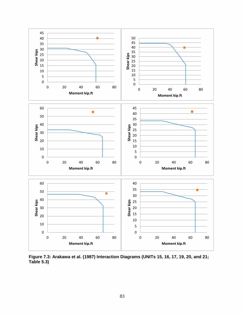
83

Figure 7.3: Arakawa et al. (1987) Interaction Diagrams (UNITs 15, 16, 17, 19, 20, and 21; Table 5.3)

05

1015202530354045

0 20 40 60 80

Shea

r kip

s

Moment kip.ft

05

101520253035404550

0 20 40 60 80

Shea

r kip

s

Moment kip.ft

0

10

20

30

40

50

60

0 20 40 60 80

Shea

r kip

s

Moment kip.ft

05

1015202530354045

0 20 40 60 80

Shea

r kip

s

Moment kip.ft

0

10

20

30

40

50

60

0 20 40 60 80

Shea

r kip

s

Moment kip.ft

05

10152025303540

0 20 40 60 80

Shea

r kip

s

Moment kip.ft

84

Figure 7.4: Arakawa et al. (1987) Interaction Diagrams (UNITs 23, 24, 25, 26, 27, and 28; Table 5.3)

0

10

20

30

40

50

60

70

0 50 100 150

Shea

r kip

s

Moment kip.ft

0

10

20

30

40

50

60

0 20 40 60 80

Shea

r kip

s

Moment kip.ft

0

10

20

30

40

50

0 20 40 60 80

Shea

r kip

s

Moment kip.ft

05

1015202530354045

0 20 40 60 80 100

Shea

r kip

s

Moment kip.ft

05

1015202530354045

0 20 40 60 80

Shea

r kip

s

Moment kip.ft

0

10

20

30

40

50

60

0 20 40 60 80 100

Shea

r kip

s

Moment kip.ft

85

Figure 7.5: Calderone et al. (2001) Interaction Diagrams (Table 5.4)

Figure 7.6: Henry and Mahin (1999) Interaction Diagrams (Table 5.5)

0

50

100

150

200

250

0 200 400 600 800

Shea

r kip

s

Moment kip.ft

0

50

100

150

200

250

0 200 400 600 800

Shea

r kip

s

Moment kip.ft

0

50

100

150

200

250

0 200 400 600 800 1000

Shea

r kip

s

Moment kip.ft

0

50

100

150

200

0 200 400 600 800

Shea

r kip

s

Moment kip.ft

0

20

40

60

80

100

120

140

0 200 400 600

Shea

r kip

s

Moment kip.ft

86

Figure 7.7: Hamilton et al. (2002) Interaction Diagrams (Table 5.6)

05

10152025303540

0 50 100 150

Shea

r kip

s

Moment kip.ft

05

10152025303540

0 50 100 150

Shea

r kip

s

Moment kip.ft

05

1015202530354045

0 50 100 150

Shea

r kip

s

Moment kip.ft

0

10

20

30

40

50

60

0 50 100 150

Shea

r kip

s

Moment kip.ft

0

10

20

30

40

50

60

0 50 100 150

Shea

r kip

s

Moment kip.ft

0

10

20

30

40

50

60

0 50 100 150 200

Shea

r kip

s

Moment kip.ft

87

Figure 7.8: Cheok and Stone (1986) Interaction Diagrams (Table 5.7)

Figure 7.9: Chai et al. (1991) Interaction Diagrams (Table 5.8)

0

200

400

600

800

1000

1200

0 2000 4000 6000 8000 10000

Shea

r kip

s

Moment kip.ft

0200400600800

1000120014001600

0 5000 10000 15000

Shea

r kip

s

Moment kip.ft

0

20

40

60

80

100

120

140

0 200 400 600

Shea

r kip

s

Moment kip.ft

0

20

40

60

80

100

120

140

0 200 400 600 800

Shea

r kip

s

Moment kip.ft

0

20

40

60

80

100

120

140

0 200 400 600 800

Shea

r kip

s

Moment kip.ft

88

Figure 7.10: Siryo (1975) Interaction Diagrams (Table 5.9)

0

10

20

30

40

50

60

0 50 100 150

Shea

r kip

s

Moment kip.ft

0

5

10

15

20

25

30

0 10 20 30 40

Shea

r kip

s

Moment kip.ft

0

10

20

30

40

50

60

0 20 40 60

Shea

r kip

s

Moment kip.ft

05

1015202530354045

0 10 20 30 40

Shea

r kip

s

Moment kip.ft

05

1015202530354045

0 10 20 30 40

Shea

r kip

s

Moment kip.ft

0

5

10

15

20

25

0 10 20 30 40 50

Shea

r kip

s

Moment kip.ft

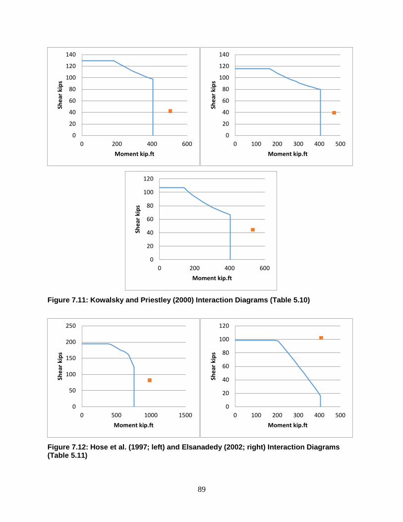
89

Figure 7.11: Kowalsky and Priestley (2000) Interaction Diagrams (Table 5.10)

Figure 7.12: Hose et al. (1997; left) and Elsanadedy (2002; right) Interaction Diagrams (Table 5.11)

0

20

40

60

80

100

120

140

0 200 400 600

Shea

r kip

s

Moment kip.ft

0

20

40

60

80

100

120

140

0 100 200 300 400 500

Shea

r kip

s

Moment kip.ft

0

20

40

60

80

100

120

0 200 400 600

Shea

r kip

s

Moment kip.ft

0

50

100

150

200

250

0 500 1000 1500

Shea

r kip

s

Moment kip.ft

0

20

40

60

80

100

120

0 100 200 300 400 500

Shea

r kip

s

Moment kip.ft

90

Figure 7.13: Moyer and Kowalsky (2003) Interaction Diagrams (Table 5.12)

Figure 7.14: Ng et al. (2010) Interaction Diagrams (Table 5.13)

0

20

40

60

80

100

0 100 200 300

Shea

r kip

s

Moment kip.ft

0

20

40

60

80

100

0 100 200 300 400

Shea

r kip

s

Moment kip.ft

0

20

40

60

80

100

0 100 200 300 400

Shea

r kip

s

Moment kip.ft

0

20

40

60

80

100

0 100 200 300

Shea

r kip

s

Moment kip.ft

0

5

10

15

20

25

30

0 10 20 30 40

Shea

r kip

s

Moment kip.ft

05

1015202530354045

0 20 40 60

Shea

r kip

s

Moment kip.ft

91

Figure 7.15: Kunnath et al. (1997) Interaction Diagrams (UNITs A2-A7; Table 5.14)

0

10

20

30

40

50

0 20 40 60 80

Shea

r kip

s

Moment kip.ft

0

10

20

30

40

50

0 20 40 60 80 100

Shea

r kip

s

Moment kip.ft

0

10

20

30

40

50

0 20 40 60 80 100

Shea

r kip

s

Moment kip.ft

0

10

20

30

40

50

0 20 40 60 80 100

Shea

r kip

s

Moment kip.ft

0

10

20

30

40

50

0 20 40 60 80 100

Shea

r kip

s

Moment kip.ft

0

10

20

30

40

50

0 20 40 60 80 100

Shea

r kip

s

Moment kip.ft

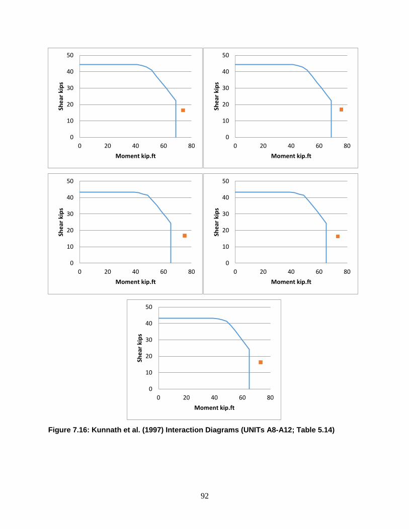
92

Figure 7.16: Kunnath et al. (1997) Interaction Diagrams (UNITs A8-A12; Table 5.14)

0

10

20

30

40

50

0 20 40 60 80

Shea

r kip

s

Moment kip.ft

0

10

20

30

40

50

0 20 40 60 80

Shea

r kip

s

Moment kip.ft

0

10

20

30

40

50

0 20 40 60 80

Shea

r kip

s

Moment kip.ft

0

10

20

30

40

50

0 20 40 60 80

Shea

r kip

s

Moment kip.ft

0

10

20

30

40

50

0 20 40 60 80

Shea

r kip

s

Moment kip.ft

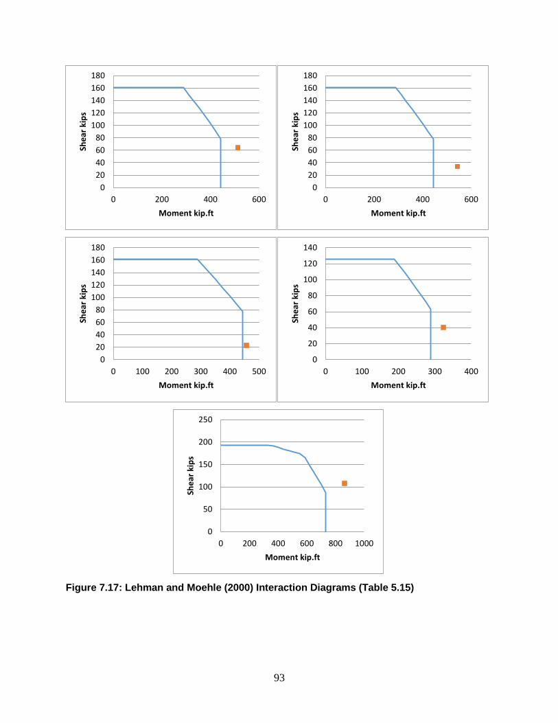
93

Figure 7.17: Lehman and Moehle (2000) Interaction Diagrams (Table 5.15)

020406080

100120140160180

0 200 400 600

Shea

r kip

s

Moment kip.ft

020406080

100120140160180

0 200 400 600

Shea

r kip

s

Moment kip.ft

020406080

100120140160180

0 100 200 300 400 500

Shea

r kip

s

Moment kip.ft

0

20

40

60

80

100

120

140

0 100 200 300 400

Shea

r kip

s

Moment kip.ft

0

50

100

150

200

250

0 200 400 600 800 1000

Shea

r kip

s

Moment kip.ft

94

Figure 7.18: Lim and McLean (1991) Interaction Diagrams (Table 5.16)

Figure 7.19: Munro et al. (1976; left) and Iwasaki et al. (1986; right) Interaction Diagrams (Table 5.17)

0

5

10

15

20

25

0 5 10 15 20

Shea

r kip

s

Moment kip.ft

0

5

10

15

20

25

0 5 10 15 20

Shea

r kip

s

Moment kip.ft

0

5

10

15

20

25

30

0 5 10 15 20

Shea

r kip

s

Moment kip.ft

0

20

40

60

80

100

120

0 100 200 300

Shea

r kip

s

Moment kip.ft

0

20

40

60

80

100

0 100 200 300 400

Shea

r kip

s

Moment kip.ft

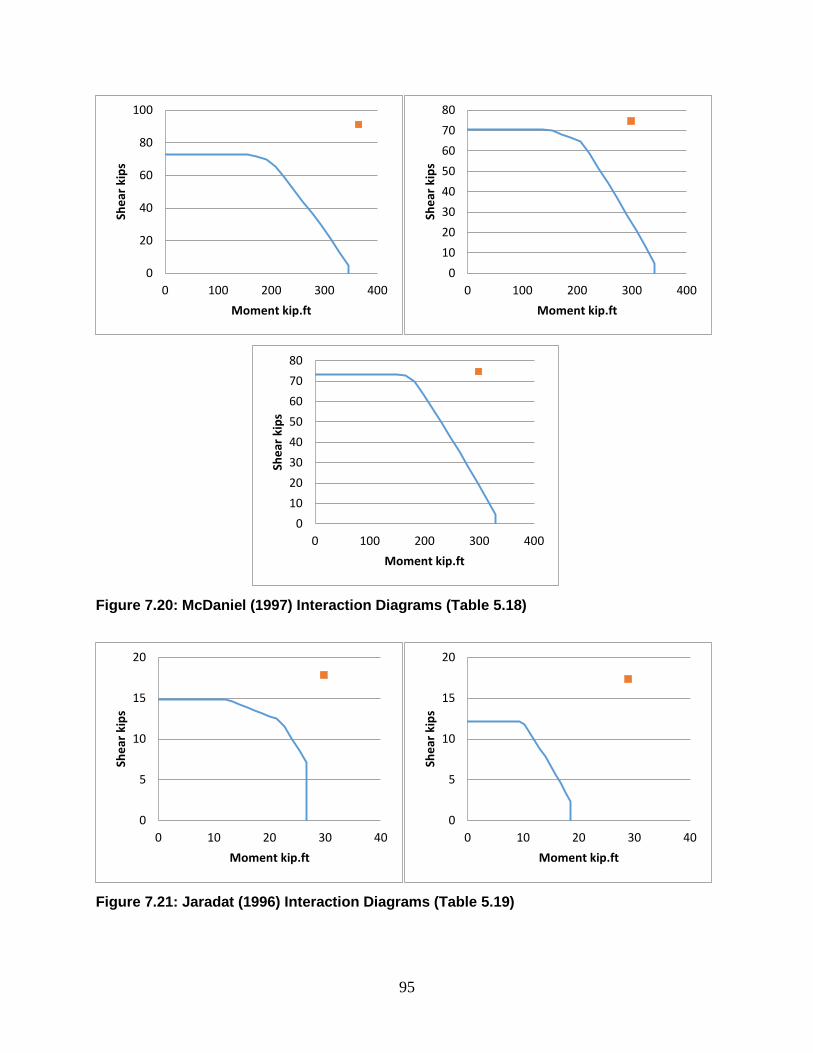
95

Figure 7.20: McDaniel (1997) Interaction Diagrams (Table 5.18)

Figure 7.21: Jaradat (1996) Interaction Diagrams (Table 5.19)

0

20

40

60

80

100

0 100 200 300 400

Shea

r kip

s

Moment kip.ft

01020304050607080

0 100 200 300 400

Shea

r kip

s

Moment kip.ft

01020304050607080

0 100 200 300 400

Shea

r kip

s

Moment kip.ft

0

5

10

15

20

0 10 20 30 40

Shea

r kip

s

Moment kip.ft

0

5

10

15

20

0 10 20 30 40

Shea

r kip

s

Moment kip.ft

96

Figure 7.22: Nelson (2000) Interaction Diagrams (Table 5.20)

Figure 7.23: Priestley et al. (1994) Interaction Diagrams (Table 5.21)

0

20

40

60

80

100

120

0 100 200 300 400

Shea

r kip

s

Moment kip.ft

0

20

40

60

80

100

120

0 100 200 300 400

Shea

r kip

s

Moment kip.ft

0

20

40

60

80

100

0 100 200 300 400

Shea

r kip

s

Moment kip.ft

0

20

40

60

80

100

120

0 100 200 300 400

Shea

r kip

s

Moment kip.ft

0

20

40

60

80

100

0 100 200 300

Shea

r kip

s

Moment kip.ft

0

20

40

60

80

100

120

140

0 100 200 300 400 500

Shea

r kip

s

Moment kip.ft

97

Figure 7.24: Petrovski and Ristic (1984) Interaction Diagrams (Table 5.22)

Figure 7.25: Zahn et al. (1986) Interaction Diagrams (Table 5.23)

0

5

10

15

20

25

30

0 10 20 30 40 50

Shea

r kip

s

Moment kip.ft

0

5

10

15

20

25

30

35

0 20 40 60

Shea

r kip

s

Moment kip.ft

0

5

10

15

20

25

30

0 20 40 60

Shea

r kip

s

Moment kip.ft

0

5

10

15

20

25

30

35

0 20 40 60 80

Shea

r kip

s

Moment kip.ft

01020304050607080

0 100 200

Shea

r kip

s

Moment kip.ft

zahn 5

Failure

0

20

40

60

80

100

120

140

0 100 200 300

Shea

r kip

s

Moment kip.ft

zahn 6

Failure

98

Figure 7.26: Pontangaroa et al. (1979) Interaction Diagrams (Table 5.24)

Figure 7.27: Watson and Park (1994) Interaction Diagrams (Table 5.25)

020406080

100120140160180

0 200 400 600 800

Shea

r kip

s

Moment kip.ft

0

50

100

150

200

250

0 200 400 600 800

Shea

r kip

s

Moment kip.ft

0

50

100

150

200

250

300

350

0 200 400 600 800

Shea

r kip

s

Moment kip.ft

050

100150200250300350400

0 200 400 600 800 1000

Shea

r kip

s

Moment kip.ft

0

20

40

60

80

100

120

140

0 100 200 300

Shea

r kip

s

Moment kip.ft

020406080

100120140160180

0 100 200 300

Shea

r kip

s

Moment kip.ft

99

Figure 7.28: Ranf et al. (2006) Interaction Diagrams (Table 5.26)

Figure 7.29: Yalcin (1997; left) and Yarandi (2007; right) Interaction Diagrams (Table 5.27)

01020304050607080

0 100 200 300

Shea

r kip

s

Moment kip.ft

0

20

40

60

80

100

0 100 200 300 400

Shea

r kip

s

Moment kip.ft

0

20

40

60

80

100

0 100 200 300 400

Shea

r kip

s

Moment kip.ft

0102030405060708090

0 100 200 300 400

Shea

r kip

s

Moment kip.ft

0

20

40

60

80

100

120

140

0 200 400 600 800

Shea

r kip

s

Moment kip.ft

0

20

40

60

80

100

120

0 100 200 300 400 500

Shea

r kip

s

Moment kip.ft

100

Figure 7.30: Roeder et al. (2001) Interaction Diagrams (Units C1-C6; Table 5.28)

0

20

40

60

80

100

0 50 100 150 200

Shea

r kip

s

Moment kip.ft

0

20

40

60

80

100

0 50 100 150 200

Shea

r kip

s

Moment kip.ft

0

20

40

60

80

100

0 50 100 150 200 250

Shea

r kip

s

Moment kip.ft

0

20

40

60

80

100

120

140

0 100 200 300

Shea

r kip

s

Moment kip.ft

0

20

40

60

80

100

120

140

0 100 200 300

Shea

r kip

s

Moment kip.ft

0

20

40

60

80

100

120

140

0 100 200 300

Shea

r kip

s

Moment kip.ft

101

Figure 7.31: Roeder et al. (2001) Interaction Diagrams (Units C7, C8; Table 5.28)

Figure 7.32: Sritharan et al. (2001) Interaction Diagrams (Table 5.29)

0

20

40

60

80

100

120

140

0 100 200 300

Shea

r kip

s

Moment kip.ft

0

20

40

60

80

100

120

140

0 100 200 300 400

Shea

r kip

s

Moment kip.ft

0

20

40

60

80

100

120

140

0 200 400 600 800

Shea

r kip

s

Moment kip.ft

0

20

40

60

80

100

120

140

0 200 400 600 800

Shea

r kip

s

Moment kip.ft

0

20

40

60

80

100

120

140

0 200 400 600 800

Shea

r kip

s

Moment kip.ft

102

Figure 7.33: Stone and Cheok (1989) Interaction Diagrams (Table 5.30)

05

10152025303540

0 10 20 30 40

Shea

r kip

s

Moment kip.ft

05

10152025303540

0 10 20 30 40 50

Shea

r kip

s

Moment kip.ft

0

5

10

15

20

25

30

0 10 20 30 40

Shea

r kip

s

Moment kip.ft

05

10152025303540

0 10 20 30 40

Shea

r kip

s

Moment kip.ft

05

10152025303540

0 10 20 30 40 50

Shea

r kip

s

Moment kip.ft

0

5

10

15

20

25

30

0 10 20 30 40

Shea

r kip

s

Moment kip.ft

103

Figure 7.34: Vu et al. (1998) Interaction Diagrams (Table 5.31)

020406080

100120140160

0 100 200 300 400 500

Shea

r kip

s

Moment kip.ft

0

20

40

60

80

100

120

140

0 100 200 300 400

Shea

r kip

s

Moment kip.ft

0

50

100

150

200

250

0 200 400 600 800

Shea

r kip

s

Moment kip.ft

0

50

100

150

200

250

300

0 200 400 600 800

Shea

r kip

s

Moment kip.ft

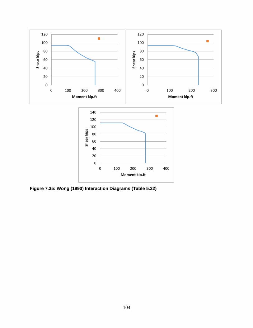
104

Figure 7.35: Wong (1990) Interaction Diagrams (Table 5.32)

0

20

40

60

80

100

120

0 100 200 300 400

Shea

r kip

s

Moment kip.ft

0

20

40

60

80

100

120

0 100 200 300

Shea

r kip

s

Moment kip.ft

0

20

40

60

80

100

120

140

0 100 200 300 400

Shea

r kip

s

Moment kip.ft

105

Figure 7.36: Ang et al. (1985) Interaction Diagrams (UNITs 1-6; Table 5.33)

01020304050607080

0 50 100 150 200

Shea

r kip

s

Moment kip.ft

0

10

20

30

40

50

60

0 50 100 150

Shea

r kip

s

Moment kip.ft

0

10

20

30

40

50

60

70

0 50 100 150 200 250

Shea

r kip

s

Moment kip.ft

0

10

20

30

40

50

60

70

0 50 100 150 200

Shea

r kip

s

Moment kip.ft

01020304050607080

0 50 100 150 200 250

Shea

r kip

s

Moment kip.ft

0

20

40

60

80

100

0 50 100 150 200

Shea

r kip

s

Moment kip.ft

106

Figure 7.37: Ang et al. (1985) Interaction Diagrams (UNITs 7-12; Table 5.33)

0

10

20

30

40

50

60

70

0 50 100 150 200

Shea

r kip

s

Moment kip.ft

0

20

40

60

80

100

120

0 100 200 300

Shea

r kip

s

Moment kip.ft

0

20

40

60

80

100

0 100 200 300 400

Shea

r kip

s

Moment kip.ft

0

20

40

60

80

100

120

0 100 200 300

Shea

r kip

s

Moment kip.ft

0

20

40

60

80

100

0 100 200 300

Shea

r kip

s

Moment kip.ft

0

20

40

60

80

100

120

140

0 50 100 150 200 250

Shea

r kip

s

Moment kip.ft

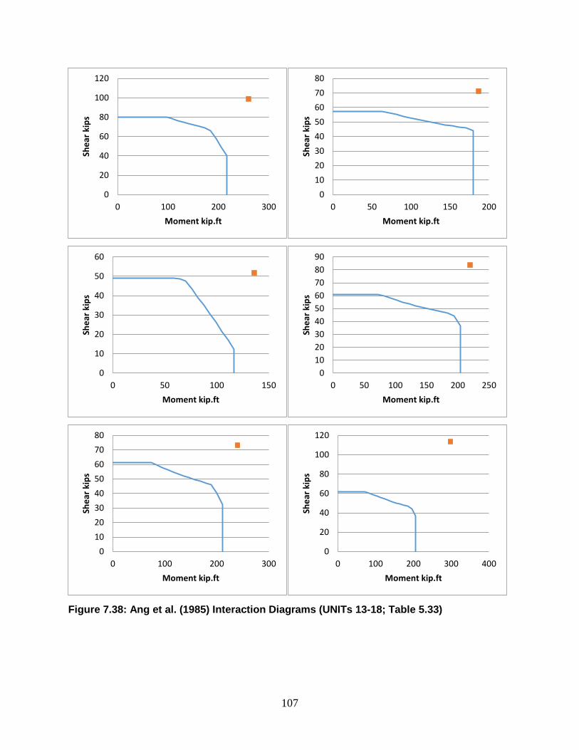
107

Figure 7.38: Ang et al. (1985) Interaction Diagrams (UNITs 13-18; Table 5.33)

0

20

40

60

80

100

120

0 100 200 300

Shea

r kip

s

Moment kip.ft

01020304050607080

0 50 100 150 200

Shea

r kip

s

Moment kip.ft

0

10

20

30

40

50

60

0 50 100 150

Shea

r kip

s

Moment kip.ft

0102030405060708090

0 50 100 150 200 250

Shea

r kip

s

Moment kip.ft

01020304050607080

0 100 200 300

Shea

r kip

s

Moment kip.ft

0

20

40

60

80

100

120

0 100 200 300 400

Shea

r kip

s

Moment kip.ft

108

Figure 7.39: Ang et al. (1985) Interaction Diagrams (UNITs 19-24; Table 5.33)

0

20

40

60

80

100

120

0 50 100 150 200 250

Shea

r kip

s

Moment kip.ft

0

20

40

60

80

100

120

0 100 200 300

Shea

r kip

s

Moment kip.ft

0

10

20

30

40

50

60

70

0 50 100 150 200

Shea

r kip

s

Moment kip.ft

0

10

20

30

40

50

60

70

0 50 100 150 200

Shea

r kip

s

Moment kip.ft

01020304050607080

0 50 100 150 200 250

Shea

r kip

s

Moment kip.ft

0102030405060708090

0 50 100 150 200 250

Shea

r kip

s

Moment kip.ft

109

Chapter 8: Conclusions

In this study, a formulation conforming to AASHTO (2014) LRFD Bridge Construction

Specifications is developed to predict the axial force-shear-moment interaction diagrams of

circular confined concrete bridge pier sections. Comparisons with a large database of

experiments indicate the accuracy of the resulting diagrams. A further step was taken to improve

the accuracy of the calculations.

Transverse steel area, spacing, cross section diameter, and applied axial force are the

main keys to analyze and increase the shear capacity of the cross section. Treating the cracked

concrete as a new different material proved to be a beneficial approach to predict the capacities

and behaviors of sections.

On the other hand, comparisons against the AASHTO (1999) interaction diagram option

in Response 2000 show that the latter yields incorrect predictions in moment-dominated failure.

The author suggests that appropriate corrections be made to Response 2000 to correct these

interaction diagram errors. The reader is also directed to use KDOT Column Expert for more

accurate prediction of the interaction diagrams.

110

References

Abd El-Fattah, A.M., Rasheed, H.A., & Esmaeily, A. (2011). A new eccentricity-based

simulation to generate ultimate confined interaction diagrams for circular concrete

columns. Journal of the Franklin Institute, 348(7), 1163-1176.

ACI Committee 318. (2011). Building code requirements for structural concrete (ACI 318-11).

Farmington Hills, MI: American Concrete Institute.

American Association of State Highway and Transportation Officials (AASHTO). (1999).

AASHTO LRFD Bridge Construction Specifications (1999 Interim Edition).

Washington, DC: Author.

American Association of State Highway and Transportation Officials (AASHTO). (2014).

AASHTO LRFD Bridge Design Specifications (7th ed.). Washington, DC: Author.

Ang, B.G., Priestley, M.J.N., & Paulay, T. (1985). Seismic shear strength of circular bridge piers

(Report 85-5). Christchurch, New Zealand: University of Canterbury.

Ang, B.G., Priestley, M.J.N., & Paulay, T. (1989). Seismic shear strength of circular reinforced

concrete columns. ACI Structural Journal, 86(1), 45-59.

Arakawa, T., He, M.X., Arai, Y., & Mizoguchi, M. (1987). Ultimate shear strength of spirally-

confined concrete columns. Transactions of the Japan Concrete Institute, 9, 305-312.

Bentz, E.C., Vecchio, F.J., & Collins, M.P. (2006). Simplified modified compression field theory

for calculating shear strength of reinforced concrete elements. ACI Structural Journal,

103(4), 614-624.

Calderone, A.J., Lehman, D.E., & Moehle, J.P. (2001). Behavior of reinforced concrete bridge

columns having varying aspect ratios and varying lengths of confinement (PEER Report

2000/08). Berkeley, CA: Pacific Earthquake Engineering Research Center.

California Department of Transportation (Caltrans). (2010). Seismic retrofit guidelines for

bridges in California (Caltrans Memo to Designers 20-4). Retrieved from

http://www.dot.ca.gov/hq/esc/techpubs/manual/bridgemanuals/bridge-memo-to-

designer/bmd.html

111

Chai, Y.H., Priestley, M.J.N., & Seible, F. (1991). Seismic retrofit of circular bridge columns for

enhanced flexural performance. ACI Structural Journal, 88(5), 572-584.

Cheok, G.S., & Stone, W.C. (1986). Behavior of 1/6-scale model bridge columns subjected to

cyclic inelastic loading. Gaithersburg, MD: US Department of Commerce, National

Bureau of Standards.

Elsanadedy, H.M. (2002). Seismic performance and analysis of ductile composite-jacketed

reinforced concrete bridge columns (Doctoral dissertation). University of California,

Irvine, CA.

Hamilton, C.H., Pardoen, G.C., & Kazanjy, R.P. (2002). Experimental testing of bridge columns

subjected to reversed-cyclic and pulse-type loading histories (Report 2001-03, Civil

Engineering Technical Report Series). Irvine, CA: University of California.

Henry, L., & Mahin, S.A. (1999). Study of buckling of longitudinal bars in reinforced concrete

bridge columns. Sacramento, CA: California Department of Transportation.

Hose, Y.D., Seible, F., & Priestley, M.J.N. (1997). Strategic relocation of plastic hinges in

bridge columns (Structural Systems Research Project Report No. SSRP-97/05). La Jolla,

CA: University of California, San Diego.

Iwasaki, T., Kawashima, K., Hagiwara, R., Hasegawa, K., Koyama, T., & Yoshida, T. (1986).

Experimental investigation on hysteretic behavior of reinforced concrete bridge pier

columns. In Raufaste, N.J. (Ed.), Wind and seismic effects: Proceedings of the 17th Joint

Panel Meeting of the U.S.-Japan Cooperative Program in Wind and Seismic Effects, May

21-24, 1985. Gaithersburg, MD: Center for Building Technology, U.S. National Bureau

of Standards.

Jaradat, O.A. (1996). Seismic evaluation of existing bridge columns (Doctoral dissertation).

Washington State University, Pullman, WA.

Joint ASCE-ACI Task Committee 426. (1973). Shear strength of reinforced concrete members.

Journal of the Structural Division, 99(6), 1091-1187.

Kowalsky, M.J., & Priestley, M.J.N. (2000). Improved analytical model for shear strength of

circular reinforced concrete columns in seismic regions. ACI Structural Journal, 97(3),

388-396.

112

Kunnath, S.K., El-Bahy, A., Taylor, A.W., & Stone, W.C. (1997). Cumulative seismic damage of

reinforced concrete bridge piers (NCEER Technical Report 97-0006). Buffalo, NY: US

National Center for Earthquake Engineering Research.

Lehman, D.E., & Moehle, J.P. (2000). Seismic performance of well-confined concrete bridge

columns (PEER Report 1998/01). Berkeley, CA: Pacific Earthquake Engineering

Research Center.

Lim, K.Y., & McLean, D.I. (1991). Scale model studies of moment-reducing hinge details in

bridge columns. ACI Structural Journal, 88(4), 465-474.

McDaniel, C.C. (1997). Scale effects on the shear strength of circular reinforced concrete

columns (Master’s thesis). University of California, San Diego, La Jolla, CA.

Moyer, M.J., & Kowalsky, M.J. (2003). Influence of tension strain on buckling of reinforcement

in RC bridge columns. ACI Structural Journal, 100(1), 75-85.

Munro, I.R.M., Park, R., & Priestley, M.J.N. (1976). Seismic behavior of reinforced concrete

bridge piers (Report 76-9). Christchurch, New Zealand: University of Canterbury.

Nelson, J.M. (2000). Damage model calibration for reinforced concrete columns (Master's

thesis). University of Washington, Seattle, WA.

Ng, P.L., Lam, J.Y.K., & Kwan, A.K.H. (2010). Tension stiffening in concrete beams. Part 1: FE

analysis. Proceedings of the Institution of Civil Engineers: Structures and Buildings,

163(1), 19-28.

Nutt, R.V. (1996). Improved seismic design criteria for California bridges: Provisional

recommendations (Report No. ATC-32). Redwood City, CA: Applied Technology

Council.

Ohtaki, T., Benzoni, G., & Priestley M.J.N. (1996). Seismic performance of a full-scale bridge

column—as built and as repaired (Structural Systems Research Project Report No.

SSRP-96/07). La Jolla, CA: University of California, San Diego.

Petrovski, J., & Ristic, D. (1984). Reversed cyclic loading test of bridge column models (Report

IZIIS 84-164). Skopje, Republic of Macedonia: Institute of Earthquake Engineering and

Engineering Seismology.

113

Pontangaroa, R.T., Priestley, M.J.N., & Park, R. (1979). Ductility of spirally reinforced concrete

columns under seismic loading (Report 79-8). Christchurch, New Zealand: University of

Canterbury.

Priestley, M.J.N., Verma, R., & Xiao, Y. (1994). Seismic shear strength of reinforced concrete

columns. Journal of Structural Engineering, 120(8), 2310-2329.

Ranf, R.T., Eberhard, M.O., & Stanton, J.F. (2006). Effects of displacement history on failure of

lightly confined bridge columns. American Concrete Institute Special Publication, 236,

23-42.

Rasheed, H.A., Abd El-Fattah, A.M., Esmaeily, A., Jones, J.P., & Hurst, K.F. (2012). Software

for adaptable eccentric analysis of confined concrete circular columns. Computers and

Concrete, 10(4), 331-347.

Roeder, C.W., Graff, R., Soderstrom, J.L., & Yoo, J.H. (2001). Seismic performance of pile-

wharf connections (PEER Report 2002/07). Berkeley, CA: Pacific Earthquake

Engineering Research Center.

Saatcioglu, M., & Baingo, D. (1999). Circular high-strength concrete columns under simulated

seismic loading. Journal of Structural Engineering, 125(3), 272-280.

Shahrooz, B.M., Miller, R.A., Harries, K.A. & Russell, H.G. (2011). Design of concrete

structures using high-strength steel reinforcement (NCHRP Report 679). Washington,

DC: Transportation Research Board.

Siryo, K.K. (1975). Aseismic analysis of building structural members: A list of experimental

results on deformation ability of reinforced concrete columns under large deflection (No.

2). Japan: Building Research Institute, Ministry of Construction.

Sritharan, S., Priestley, M.J.N., & Seible, F. (2001). Seismic design and experimental

verification of concrete multiple column bridge bents. ACI Structural Journal, 98(3),

335-346.

Standards New Zealand. (1995). Design of concrete structures. In Concrete Structures Standard

(NZS 3101). Wellington, New Zealand: Author.

114

Stone, W.C., & Cheok, G.S. (1989). Inelastic behavior of full-scale bridge columns subjected to

cyclic loading (NIST BSS 166). Gaithersburg, MD: National Institute of Standards and

Technology.

Vecchio, F.J., & Collins, M.P. (1986). The modified compression-field theory for reinforced

concrete elements subjected to shear. ACI Journal Proceedings, 83(2), 219-231.

Vu, N.D., Priestley, M.J.N., Seible, F., & Benzoni, G. (1998, June). Seismic response of well

confined circular reinforced concrete columns with low aspect ratios. Paper presented at

the meeting of the 5th Caltrans Seismic Research Workshop, Sacramento, CA.

Walraven, J.C. (1981). Fundamental analysis of aggregate interlock. Journal of the Structural

Division, 107(11), 2245-2270.

Watson, S., & Park, R. (1994). Simulated seismic load tests on reinforced concrete columns.

Journal of Structural Engineering, 120(6), 1825-1849.

Wong, Y.L. (1990). Squat circular bridge piers under multi-directional seismic attack (Doctoral

dissertation). University of Canterbury, Christchurch, New Zealand.

Yalcin, C. (1997). Seismic evaluation and retrofit of existing reinforced concrete bridge columns

(Doctoral dissertation). University of Ottawa, Ottawa, Canada.

Yarandi, M.S. (2007). Seismic retrofit and repair of existing reinforced concrete bridge columns

by transverse prestressing (Doctoral dissertation). University of Ottawa, Ottawa, Canada.

Zahn, F.A., Park, R., & Priestley, M.J.N. (1986). Design of reinforced concrete bridge columns

for strength and ductility (Report 86-7). Christchurch, New Zealand: University of

Canterbury.