K-Dominant Skyline Join Queries: Extending the JoinParadigm to K-Dominant Skylines

Anuradha Awasthi Arnab Bhattacharya Sanchit Gupta Ujjwal Kumar SinghDept. of Computer Science and Engineering, Indian Institute of Technology, Kanpur, India

{aawasthi,arnabb,sanchitg,ujjkumsi}@cse.iitk.ac.in

ABSTRACTSkyline queries enable multi-criteria optimization by filtering ob-jects that are worse in all the attributes of interest than anotherobject. To handle the large answer set of skyline queries in high-dimensional datasets, the concept of k-dominance was proposedwhere an object is said to dominate another object if it is better(or equal) in at least k attributes. This relaxes the full dominationcriterion of normal skyline queries and, therefore, produces lessernumber of skyline objects. This is called the k-dominant skylineset. Many practical applications, however, require that the prefer-ences are applied on a joined relation. Common examples includeflights having one or multiple stops, a combination of product priceand shipping costs, etc. In this paper, we extend the k-dominantskyline queries to the join paradigm by enabling such queries to beasked on joined relations. We call such queries KSJQ (k-dominantskyline join queries). The number of skyline attributes, k, that anobject must dominate is from the combined set of skyline attributesof the joined relation. We show how pre-processing the base re-lations helps in reducing the time of answering such queries overthe naïve method of joining the relations first and then running thek-dominant skyline computation. We also extend the query to han-dle cases where the skyline preference is on aggregated values inthe joined relation (such as total cost of the multiple legs of theflight) which are available only after the join is performed. In ad-dition to these problems, we devise efficient algorithms to choosethe value of k based on the desired cardinality of the final skylineset. Experiments on both real and synthetic datasets demonstratethe efficiency, scalability and practicality of our algorithms.

KeywordsSkyline query; K-dominant skyline query; Join; Aggregation; K-dominant skyline join query; KSJQ

1. INTRODUCTION AND MOTIVATIONSkyline queries are widely used to enable multi-criteria decision

making in databases [3]. Consider a scenario where a person wantsto buy a good house. Her preferences are low cost, proximity tomarket, quiet neighborhood, etc. In a real scenario, it is almost

ACM ISBN XXX.

DOI: XXX

impossible to find a single house that is best in all her preferences.The skyline query helps her narrow down the choices by filteringout houses that are worse (or equal) than some other house in all thepreferences. Assuming rationality, her choices cannot lie outsidethe skyline set.

In high-dimensional spaces, however, the skyline set becomesless useful due to its impractically large size. The size tends toincrease exponentially with dimensionality [28]. This happens as itbecomes harder for any object to dominate another object in all theattributes. The problem is especially severe in real datasets wherethe data is generally anti-correlated in nature. For example, a quietneighborhood closer to a market is likely to be more costly.

There have been various works on handling the large cardinalityof skyline sets in high dimensions. The most prominent is that ofk-dominant skylines where, instead of being better in all the d di-mensions, an object need only be better in some k < d dimensionsto dominate another object [4]. As a result, it becomes easier for anobject to be dominated which leads to lesser number of skylines.

The k-dominant skylines are quite useful in real scenarios. In theexample of housing discussed above, if there are many attributes, itmay be rare that one house is better than another on all the counts.Instead, if a smaller number of attributes, say k = 2, is specified,there are more chances of finding a house that has a lower cost anda quieter neighborhood (but may not be closer to a market) thananother house. As a result, more houses can be filtered, and theretrieved skyline set becomes more manageable and useful.

To the best of our knowledge, however, the k-dominant skylinequeries have not been explored for multiple relations.1 Supposethere are two relations having d1 and d2 skyline attributes. Af-ter joining, a bigger relation with d1 + d2 skyline attributes isformed. (We discuss the different variants and restrictions later.)A k-dominant skyline, where k < d1 + d2, is then sought on thisjoined relation.

A real-life example of this situation happens often in flight book-ings. Suppose a person wants to fly from city A to city B. Her pref-erences are lower cost, lower duration, higher ratings and higheramenities. While the basic skyline works for direct flights, in manycases, a flight route from A to B includes one (or more) stopovers.Thus, a valid flight path contains the join of all flights from city Ato other cities and from those cities to city B where the intermediatecity is the same. The preferences a user would want now applies tothe entire flight path and not a single leg of the journey. The skylineis, therefore, needed on the joined relation [2, 21].

Once more, it is harder for a flight combination to dominate an-other flight combination in all the skyline attributes over the tworelations. Here, the k-dominant skyline query is a natural choice,where k is less than the total number of the skyline attributes in the

1A preliminary version of this paper will appear as a poster [1].

arX

iv:1

702.

0339

0v1

[cs

.DB

] 1

1 Fe

b 20

17

joined relation.With the increase in the number of attributes, the size of the sky-

line set increases further and, hence, computing the k-dominantskylines becomes even more relevant and useful.

The naïve approach first creates the joined relation and then sub-sequently computes the k-dominance. This strategy, while straight-forward, is inefficient and impractical for large datasets.

A further practical consideration in the flight example is that auser is not really bothered about the individual legs, but rather thetotal cost and total duration of the journey. Thus, the skyline prefer-ences should be applied on the aggregated values of attributes fromthe base relations. Note that the aggregated values are availableonly after the join and are, therefore, harder to process efficiently.

In this paper, we explore the question of finding k-dominant sky-lines on joined relations, where the skyline preferences can be onboth aggregated and individual values. Apart from posing the prob-lem, our main contribution is to push the skyline operator beforethe join as much as possible, thereby making the whole algorithmefficient and practical.

In addition to finding k-dominant skylines, an important questionthat often arises in practical applications is how to choose a “good”value of k? While there is no universal answer, one of the guidingprinciples is the number of skyline objects finally returned [4]. Thebasic idea of skyline queries is to serve as a filter for poor objectsand, thus, a user may find it easier to specify a value of δ objectsthat she is interested in examining more thoroughly rather than avalue of k. Since the size of the skyline set increases with k, the“optimal” value of k may be then taken as the smallest one thatreturns at least δ skyline objects, or the largest one that returns atmost δ skyline objects.

We address the above question in the context of k-dominant sky-lines over joined relations.

In sum, our contributions are:1. We propose the problem of finding k-dominant skyline queries

over joined relations. We term such queries KSJQ.2. We design efficient algorithms to solve the KSJQ problem.3. We devise ways to arrive at a good value of “k” by specifying

a threshold size of the k-dominant skyline set.The rest of the paper is organized as follows. Sec. 2 sets the

background on joins of k-dominant skylines. Using this, differentproblem statements are defined in Sec. 3. Sec. 4 outlines the relatedwork. Various optimizations that can improve the efficiency of theproblem are explained in Sec. 5. Algorithms that use these opti-mizations are described in Sec. 6. Sec. 7 analyzes the experimentalresults before Sec. 8 concludes.

2. BACKGROUND

2.1 SkylinesConsider a dataset R of objects. For each object u, a set of d

attributes {u1, . . . , ud} are specified, which form the skyline at-tributes. For each of the skyline attributes, without loss of gen-erality, the preference is assumed to be less than (<), i.e., a lowervalue is preferred over a higher one. An object u dominates anotherobject v, denoted by u � v, if and only if, for all the d skyline at-tributes, ui is preferred over or equal to vi, and there exists at leastone skyline attribute where uj is strictly preferred over vj . Theskyline set S ⊆ R contains objects that are not dominated by anyother object [3]. In other words, every object in the non-skyline setis dominated by at least one object in the dataset.

2.2 K-Dominant Skylines

The k-dominant skyline query [4] relaxes the definition of domi-nation between objects. An object u k-dominates another object v,denoted by u �k v, if and only if, for at least k of the d skyline at-tributes, ui is preferred over or equal to vi, and there exists at leastone skyline attribute where uj is strictly preferred over vj . Thek-dominant skyline set contains objects that are not k-dominatedby any other object. The k attributes are not fixed and can be anysubset of the d skyline attributes.

The k-dominant query is particularly problematic when k ≤ d2

since then two objects can dominate each other. Even when k >d2

, the k-dominance relationship is not transitive and may be evencyclic: u �k v �k w �k u.

2.3 Multi-Relational SkylinesConsider two datasets R1 and R2 with d1 and d2 skyline at-

tributes respectively. The join of the two relations (using appro-priate join conditions) forms the dataset R = R1 1 R2 withd = d1 + d2 skyline attributes. The multi-relational skyline isextracted from R [21].

In a significant variant of the problem, a number of skyline at-tributes in each relation are marked for aggregation with corre-sponding attributes from the other relation [2]. Thus, a attributesout of d1 in R1 and d2 in R2 are aggregated in the joined relationR. As a result, R contains (d1− a) + (d2− a) + a = d1 + d2− askyline attributes. The skyline query is then asked over these at-tributes. The aggregation function is assumed to be monotonic; thisensures that if the base values of two tuples u ∈ R1 and t ∈ R2

are preferred over the base tuples of two other tuples v ∈ R1 ands ∈ R2 respectively, the aggregated value of u 1 t ∈ R will benecessarily preferred over the aggregated value of v 1 s ∈ R.

The case for more than two base relations can be handled bycascading the joins.

3. PROBLEM STATEMENTSWe propose two main variants of what we call the K-DOMINANT

SKYLINE JOIN QUERY (KSJQ) problem.The first variant works on relations for which the skyline at-

tributes are strictly local.The number of skyline attributes in the first and second relations,

R1 and R2, are d1 and d2 respectively.

R1 = {h11 , . . . , h1m , s11 , . . . , s1d1 } (1)

R2 = {h21 , . . . , h2m , s21 , . . . , s2d2 } (2)

R = {h1, . . . , hm, s11 , . . . , s1d1 , s21 , . . . , s2d2 } (3)

where hi captures the join of h1i with h2i in the joined relationR = R1 1 R2, and s1i , s2i are the skyline attributes.

PROBLEM 1 (KSJQ). Given two datasets R1 and R2 havingd1 and d2 skyline attributes respectively, find k-dominant skylinesfrom the joined relationR = R1 1 R2 having d = d1 +d2 skylineattributes.

We restrict k to be at least one more than the dimensionality inthe base relations, i.e., max{d1, d2} < k < d. This restrictionconstrains at least some skyline attributes from each relation to sat-isfy the preferences. In other words, the k preferred attributes mustspan both the relations. However, there is no restriction over howmany skyline attributes from each relation must be satisfied. De-noting the number of skyline attributes that are chosen from thetwo relations by k1 and k2 where k1 + k2 = k, this implies that1 ≤ k1 ≤ d1 and 1 ≤ k2 ≤ d2.

The second variant works on the aggregate version of the prob-lem. Assuming a total of a aggregate attributes, the number of

attributes on which only local skyline preferences are applied ared1 − a = l1 and d2 − a = l2 respectively. The joined relation R,therefore, contains l1+l2 local attributes and a aggregate attributes.

PROBLEM 2 (AGGREGATE KSJQ). Given two datasetsR1 andR2 having d1 and d2 skyline attributes respectively, of which a at-tributes are used for aggregation, find k-dominant skylines fromthe joined relation R = R1 1 R2 having d1 + d2 − a skylineattributes.

Once more, we assume that max{d1, d2} < k ≤ d. Expressingin terms of local and aggregate attributes, max{l1, l2}+ a < k ≤l1 + l2 + a.

The third and fourth problems address the tuning of the value ofk. The value can be tuned in two ways.

PROBLEM 3 (AT LEAST δ). Given a KSJQ query frameworkand a threshold number of skyline objects δ, determine the smallestvalue of k that returns at least δ skyline objects.

PROBLEM 4 (AT MOST δ). Given a KSJQ query frameworkand a threshold number of skyline objects δ, determine the largestvalue of k that returns at most δ skyline objects.

Prob. 4 is directly linked with Prob. 3. If k∗ is the answer toProb. 3, then the answer to Prob. 4 must be k∗ − 1. There are twocorner cases. First, if k∗ = 1, then the answer to Prob. 4 should betrivially 1 as well. Second, if k∗-dominant skyline returns exactlyδ skyline objects (or k∗ = d), then the answer to Prob. 4 is k∗ aswell. Thus, henceforth, we focus only on Prob. 3.

4. RELATED WORKThe skyline operator was introduced in databases by [3] by adopt-

ing the maximal vector or the Pareto optimal problem [15]. Severalindexed [14], [17] and non-indexed algorithms [3, 5, 22] have beensince proposed to retrieve the skyline set.

Analyses of the cardinality of the skyline set [9, 28] have shownthat the number of skyline objects can grow exponentially with theincrease in dimensionality. Consequently, several attempts havebeen made to restrict the size of the skyline set. These mostly in-clude notions of approximate skylines or representative skylines [6,8, 10, 12, 13, 16, 23, 25, 26, 27].

A completely different approach—k-dominant skylines—was pro-posed by [4]. It uses subsets of skyline attributes to control the car-dinality of the skyline set. Although the parameter k is an input tothe problem, the authors also proposed a way to derive the smallestk that will guarantee a δ number of skylines.

There have been many recent works on k-dominant skylines in-cluding extensions to high-dimensional spaces [18, 19], using par-allel processing [24], cardinality estimation [11] as well as in update-heavy datasets [20] and combined datasets [7].

The skyline join problem where skylines are retrieved from joinedrelations, both components of which contain skyline attributes, wasintroduced in [21]. This work, however, simply assumed that theskyline attributes remain unchanged from the base relations to thejoined one. The aggregate skyline join queries [2] removed this re-striction by enabling skyline preferences to be posed on aggregatevalues of attributes formed by combining attributes from the baserelations. The aggregation function was assumed to be monotonic.

In this paper, we pose the k-dominant skyline problem in thejoin paradigm (including the aggregated version). To the best ofour knowledge, this is the first work in this direction.

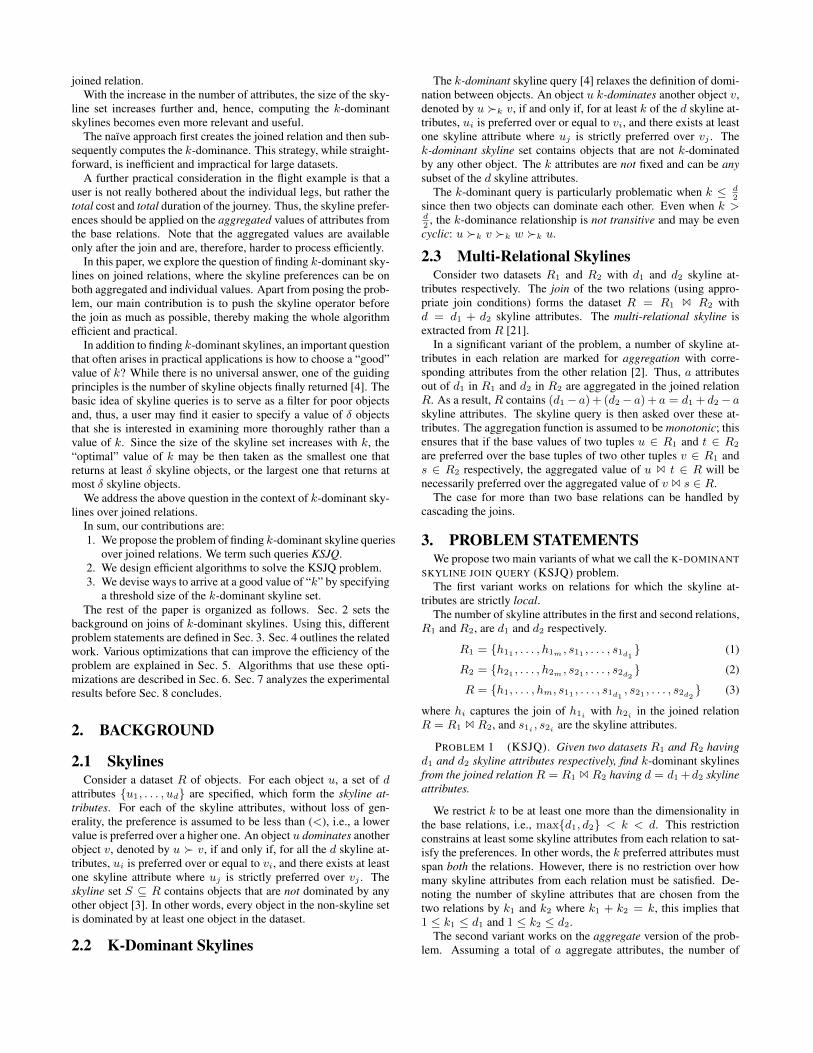
fno destination cost dur rtg amn category11 C 448 3.2 40 40 SS1

12 C 468 4.2 50 38 NN1

13 D 456 3.8 60 34 SN1

14 D 460 4.0 70 32 NN1

15 E 450 3.4 30 42 SN1

16 F 452 3.6 20 36 SS1

17 G 472 4.6 80 46 SN1

18 H 451 3.7 20 37 SS1

19 E 451 3.7 40 37 NN1

Table 1: Flights from city A (f1).

5. OPTIMIZATIONSIn this section, we describe the various optimization schemes that

can be used to speed-up the process of finding k-dominant skylinesin joined relations. Sec. 6 uses these optimizations to design thealgorithms.

5.1 Join AttributesWe assume an equality join condition. Two base tuples u ∈ R1

and v ∈ R2 can be joined to form t = u 1 v ∈ R if and only if alltheir join attributes match. Referring to Eq. (3), ∀j=1,...,m h1j =h2j . (We discuss the relaxation of this assumption in Sec. 6.6.)

ASSUMPTION 1 (EQUALITY JOIN). The join conditions areall based on equality, i.e., the join is an equality join.

All the tuples in a base relation are, thus, divided into groupsaccording to the value of the join attributes. In every group, thevalues of the join attributes, hi1 , . . . , him(i = 1, 2), are the same.

In the flight example, since the joining criterion is destinationof first flight to be the source of the second flight, the first baserelation is divided on the basis of destinations while the second oneis divided on sources.

5.2 GroupingBased on the k-dominance properties within each group, each

base relation is partitioned into different sets as follows.A tuple may be a k-dominant tuple for the entire base relation.

However, even when it is not, it may not be k-dominated by anyother tuple in its group. It is then a k-dominant tuple when only itsgroup is concerned.

Based on the above notion of k-dominance within a group, eachbase relationRi is divided into 3 mutually exclusive and exhaustivesets SSi, SNi, and NNi:

Ri = SSi ∪ SNi ∪NNi (4)

We next define the three sets.

DEFINITION 1 (SS). A tuple u is in SS if u is a k-dominantskyline in the overall relation; consequently, it is a k-dominant sky-line in its group as well.

DEFINITION 2 (SN ). A tuple u is in SN if u is a k-dominantskyline only in its group but not in the overall relation.

DEFINITION 3 (NN ). A tuple u is in NN if u is not a k-dominant skyline in its group; consequently, it is not a k-dominantskyline in the overall relation as well.

Consider the examples in Table 1 and Table 2. We assume thatall the attributes have lower preferences2. We set k = 3 for both2Although the preferences for ratings and amenities are generallythe other way round, we stick to lower preferences for ease of un-derstanding.

fno source cost dur rtg amn category21 D 348 2.2 40 36 SS2

22 D 368 3.2 50 34 NN2

23 C 356 2.8 60 30 SN2

24 C 360 3.0 70 28 NN2

25 E 350 2.4 30 38 SN2

26 F 352 2.6 20 32 SS2

27 G 372 3.6 80 42 SN2

28 H 350 2.4 35 37 SN2

Table 2: Flights to city B (f2).

the relations. The categorization of the tuples are shown in the lastcolumn.

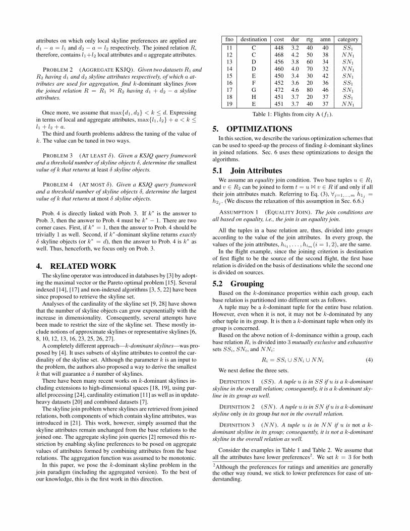
Table 3 shows the joined relation.The important outcome of this division into the three sets is that it

allows certain tuples to be automatically designated as k-dominantskylines (or not) without computing the join, as explained next.

5.3 Deciding about Skylines before JoinWe first analyze a simple case where out of the final k attributes

in the joined relation, if a joined tuple t k-dominates another joinedtuple s, t must k1-dominate s in the first base relation and mustk2-dominate in the second base relation (k = k1 + k2).

Note that, in practice this situation will not be specified by anyuser. We are only going to use it to explain the basic conceptsand then build upon it later by removing this assumption. Forthe theorems and observations in this section, the first base rela-tion is divided into the three sets SS1, SN1, NN1 according tok1-domination while the second base relation is divided into SS2,SN2, NN2 using k2-domination.

The first theorem shows that a tuple formed by joining the SScounterparts is always a k-dominant skyline.

THEOREM 1. The tuples in the set (SS1 1 SS2) are k-dominantskylines.

PROOF. Consider a joined tuple t′ = u′ 1 v′ formed by joiningthe tuples u′ ∈ SS1 and v′ ∈ SS2. Assume that t = u 1 vk-dominates t′, i.e., t �k t′. Since u′ ∈ SS1, no tuple and, inparticular, u can k1-dominate u′. Similarly, v 6�k2 v

′. Therefore,6 ∃t, t �k t

′. Hence, t′ is a k-dominant tuple.

The flight combination (16,26) in Table 3 is an example.The second theorem shows the reverse: composite tuples formed

by joining a base tuple in NN can never be k-dominant skylines.

THEOREM 2. The tuples in the sets (SS1 1 NN2), (SN1 1

NN2), (NN1 1 SS2), (NN1 1 SN2), and (NN1 1 NN2) arenot k-dominant skylines.

PROOF. Consider a joined tuple t′ = u′ 1 v′ formed by joiningthe tuples u′ ∈ NN1 and v′ ∈ R2. Therefore, there must exist atuple u in the same group that k1-dominates u′, i.e., ∃u, u �k1 u

′.Consider the tuple t formed by joining u with v′. Since u is in thesame group as u′, this tuple necessarily exists. As t dominates t′

in k1 attributes and is equal in k2, overall, it dominates in k1 +k2 = k attributes, i.e., t �k t

′. Therefore, t′ is not a k-dominantskyline. This covers the cases (NN1 1 SS2), (NN1 1 SN2),and (NN1 1 NN2). The cases for (SS1 1 NN2) and (SN1 1

NN2) are symmetrical.

The flight combinations (11,24), (13,22), (14,21), (14,22), (12,23),and (12,24) in Table 3 exemplify the above cases. For example, thetuple (11,24) is dominated by (11,23).

However, nothing can be concluded surely about the rest of thejoined tuples.

OBSERVATION 1. The tuples in the sets (SS1 1 SN2) and(SN1 1 SS2) are most likely to be k-dominant skylines, althoughthat is not guaranteed.

PROOF. Consider a joined tuple t′ = u′ 1 v′ formed by joiningthe tuples u′ ∈ SS1 and v′ ∈ SN2. Consider the dominator v ∈R2 �k2 v′. Since v′ is a k2-dominate skyline in R2, v is in adifferent group than v′. Therefore, v cannot join with u′, i.e., 6 ∃t =u′ 1 v, v �k2 v′. Although no tuple u can k1-dominate u′,there may exist u whose k1 attributes have the same value as u′.If it happens that u is join-compatible with v, then and only then,t = u 1 v exists and t �k t

′ (since it is equal in k1 and better ink2 attributes). The above situation is quite unlikely, although notimpossible. The case for (SN1 1 SS2) is symmetrical.

Thus, while (11,23) and (13,21) are k-dominant skylines, (18,28)is not (Table 3). Flight 18 has same k1 values as 19 while 28 isdominated by 25. Therefore, (18,28) is k-dominated by (19,25).

The observation for (SN1 1 SN2) is similar.

OBSERVATION 2. A tuple in the set (SN1 1 SN2) may or maynot be a k-dominant skyline.

PROOF. Consider a joined tuple t′ = u′ 1 v′ ∈ (SN1 1

SN2). Consider the tuples u and v such that u �k1 u′ and v �k2

v′. Since u′ ∈ SN1, u is in a different group than u′. Similarly, vis in a different group than v′. If and only if u and v are join com-patible, they will join to form t = u 1 v which then k-dominatest′. Otherwise, no such t exists, and t′ is a k-dominant skyline.

Consider (15,25) in Table 3. Since its dominators, flights 11 and21 respectively, are not join compatible (11 reaches city C while 21takes off from city D), the flight combination (11,21) is not valid.Consequently, no joined tuple dominates it, and (15,25) becomes ak-dominant skyline. On the other hand, for (17,27), the dominators16 and 26 do join (the city F is common) to form the tuple (16,26).As a result, (17,27) is not a k-dominant skyline.

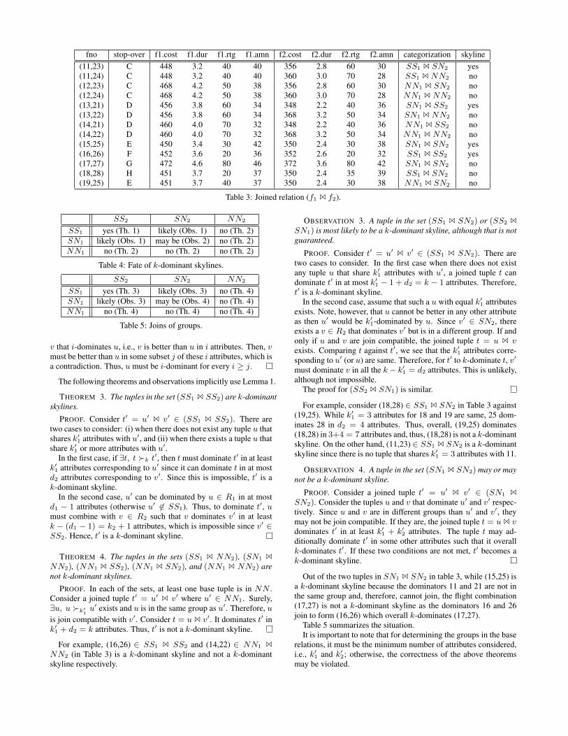
The overall situation is summed up in Table 4.

5.4 Skyline Attributes in Joined RelationWe next do away with the assumption that k1 and k2 attributes

have to be satisfied separately from the first and second relations. Itis simply required that the joined relation returns k-dominant sky-lines with no restriction on how k is broken up between the baserelations. However, to ensure that the skyline preferences are re-spected for at least one attribute in every base relation, we assumethat k > max{d1, d2}.

A brute-force way to find the skylines is to generate all combi-nations of k1 and k2 such that k1 + k2 = k and, then, combinethe answer sets using the results obtained in the previous section.However, it can be done more efficiently as explained next.

We consider the following cases:

k′1 = k − d2 k′2 = k − d1 (5)

For all combinations of k1 and k2 such that k1 + k2 = k, theinequalities, 1 ≤ k′1 ≤ k1 ≤ d1 and 1 ≤ k′2 ≤ k2 ≤ d2, hold.

Consider the example in Table 3. If k = 7, then k′1 = k′2 = 3.Thus, categorization and k-dominant skyline sets remain the same.

We first establish the following lemma on the monotonicity ofthe number of skyline attributes.

LEMMA 1. If tuple u is a j-dominant skyline, it is also a i-dominant skyline for any i ≥ j.

PROOF. Consider u to be a j-dominant tuple. Assume that,however, it is not i-dominant for some i > j. Thus, there exists

fno stop-over f1.cost f1.dur f1.rtg f1.amn f2.cost f2.dur f2.rtg f2.amn categorization skyline(11,23) C 448 3.2 40 40 356 2.8 60 30 SS1 1 SN2 yes(11,24) C 448 3.2 40 40 360 3.0 70 28 SS1 1 NN2 no(12,23) C 468 4.2 50 38 356 2.8 60 30 NN1 1 SN2 no(12,24) C 468 4.2 50 38 360 3.0 70 28 NN1 1 NN2 no(13,21) D 456 3.8 60 34 348 2.2 40 36 SN1 1 SS2 yes(13,22) D 456 3.8 60 34 368 3.2 50 34 SN1 1 NN2 no(14,21) D 460 4.0 70 32 348 2.2 40 36 NN1 1 SS2 no(14,22) D 460 4.0 70 32 368 3.2 50 34 NN1 1 NN2 no(15,25) E 450 3.4 30 42 350 2.4 30 38 SN1 1 SN2 yes(16,26) F 452 3.6 20 36 352 2.6 20 32 SS1 1 SS2 yes(17,27) G 472 4.6 80 46 372 3.6 80 42 SN1 1 SN2 no(18,28) H 451 3.7 20 37 350 2.4 35 39 SS1 1 SN2 no(19,25) E 451 3.7 40 37 350 2.4 30 38 NN1 1 SN2 no

Table 3: Joined relation (f1 1 f2).

SS2 SN2 NN2

SS1 yes (Th. 1) likely (Obs. 1) no (Th. 2)SN1 likely (Obs. 1) may be (Obs. 2) no (Th. 2)NN1 no (Th. 2) no (Th. 2) no (Th. 2)

Table 4: Fate of k-dominant skylines.

SS2 SN2 NN2

SS1 yes (Th. 3) likely (Obs. 3) no (Th. 4)SN1 likely (Obs. 3) may be (Obs. 4) no (Th. 4)NN1 no (Th. 4) no (Th. 4) no (Th. 4)

Table 5: Joins of groups.

v that i-dominates u, i.e., v is better than u in i attributes. Then, vmust be better than u in some subset j of these i attributes, which isa contradiction. Thus, u must be i-dominant for every i ≥ j.

The following theorems and observations implicitly use Lemma 1.

THEOREM 3. The tuples in the set (SS1 1 SS2) are k-dominantskylines.

PROOF. Consider t′ = u′ 1 v′ ∈ (SS1 1 SS2). There aretwo cases to consider: (i) when there does not exist any tuple u thatshares k′1 attributes with u′, and (ii) when there exists a tuple u thatshare k′1 or more attributes with u′.

In the first case, if ∃t, t �k t′, then tmust dominate t′ in at least

k′1 attributes corresponding to u′ since it can dominate t in at mostd2 attributes corresponding to v′. Since this is impossible, t′ is ak-dominant skyline.

In the second case, u′ can be dominated by u ∈ R1 in at mostd1 − 1 attributes (otherwise u′ 6∈ SS1). Thus, to dominate t′, umust combine with v ∈ R2 such that v dominates v′ in at leastk − (d1 − 1) = k2 + 1 attributes, which is impossible since v′ ∈SS2. Hence, t′ is a k-dominant skyline.

THEOREM 4. The tuples in the sets (SS1 1 NN2), (SN1 1

NN2), (NN1 1 SS2), (NN1 1 SN2), and (NN1 1 NN2) arenot k-dominant skylines.

PROOF. In each of the sets, at least one base tuple is in NN .Consider a joined tuple t′ = u′ 1 v′ where u′ ∈ NN1. Surely,∃u, u �k′

1u′ exists and u is in the same group as u′. Therefore, u

is join compatible with v′. Consider t = u 1 v′. It dominates t′ ink′1 + d2 = k attributes. Thus, t′ is not a k-dominant skyline.

For example, (16,26) ∈ SS1 1 SS2 and (14,22) ∈ NN1 1

NN2 (in Table 3) is a k-dominant skyline and not a k-dominantskyline respectively.

OBSERVATION 3. A tuple in the set (SS1 1 SN2) or (SS2 1

SN1) is most likely to be a k-dominant skyline, although that is notguaranteed.

PROOF. Consider t′ = u′ 1 v′ ∈ (SS1 1 SN2). There aretwo cases to consider. In the first case when there does not existany tuple u that share k′1 attributes with u′, a joined tuple t candominate t′ in at most k′1 − 1 + d2 = k − 1 attributes. Therefore,t′ is a k-dominant skyline.

In the second case, assume that such a u with equal k′1 attributesexists. Note, however, that u cannot be better in any other attributeas then u′ would be k′1-dominated by u. Since v′ ∈ SN2, thereexists a v ∈ R2 that dominates v′ but is in a different group. If andonly if u and v are join compatible, the joined tuple t = u 1 vexists. Comparing t against t′, we see that the k′1 attributes corre-sponding to u′ (or u) are same. Therefore, for t′ to k-dominate t, v′

must dominate v in all the k− k′1 = d2 attributes. This is unlikely,although not impossible.

The proof for (SS2 1 SN1) is similar.

For example, consider (18,28) ∈ SS1 1 SN2 in Table 3 against(19,25). While k′1 = 3 attributes for 18 and 19 are same, 25 dom-inates 28 in d2 = 4 attributes. Thus, overall, (19,25) dominates(18,28) in 3+4 = 7 attributes and, thus, (18,28) is not a k-dominantskyline. On the other hand, (11,23) ∈ SS1 1 SN2 is a k-dominantskyline since there is no tuple that shares k′1 = 3 attributes with 11.

OBSERVATION 4. A tuple in the set (SN1 1 SN2) may or maynot be a k-dominant skyline.

PROOF. Consider a joined tuple t′ = u′ 1 v′ ∈ (SN1 1

SN2). Consider the tuples u and v that dominate u′ and v′ respec-tively. Since u and v are in different groups than u′ and v′, theymay not be join compatible. If they are, the joined tuple t = u 1 vdominates t′ in at least k′1 + k′2 attributes. The tuple t may ad-ditionally dominate t′ in some other attributes such that it overallk-dominates t′. If these two conditions are not met, t′ becomes ak-dominant skyline.

Out of the two tuples in SN1 1 SN2 in table 3, while (15,25) isa k-dominant skyline because the dominators 11 and 21 are not inthe same group and, therefore, cannot join, the flight combination(17,27) is not a k-dominant skyline as the dominators 16 and 26join to form (16,26) which overall k-dominates (17,27).

Table 5 summarizes the situation.It is important to note that for determining the groups in the base

relations, it must be the minimum number of attributes considered,i.e., k′1 and k′2; otherwise, the correctness of the above theoremsmay be violated.

5.5 Unique Value PropertyFor a tuple in SS1 1 SN2 (and SN2 1 SS1) to be not a k-

dominant skyline, the number of attributes in which u ∈ R1 issame as u′ ∈ SS1 must be at least k′1. If the base relations fol-low a unique value property where it is guaranteed that for anyk′i (i = 1, 2) number of attributes, two tuples will be unique, thenthe processing becomes simpler.

DEFINITION 4 (UNIQUE VALUE PROPERTY). A relationR hasthe unique value property (UVP) with respect to i if for each sub-set of i skyline attributes of R, all the tuples are unique, i.e., notwo tuple will have exactly the same values in any i-sized subset ofattributes.

If k′i = 1, every tuple for any attribute must be unique. Whilereal-valued attributes generally follow that, categorical attributesdo not. However, for reasonable values of k′1 and k′2, real datasetshaving a mix of both real-valued and categorical attributes gener-ally follow the UVP.

The UVP is extremely useful since it ensures that the tuples inSS1 1 SN2 and SN2 1 SS1 become k-dominant skylines asshown next.

THEOREM 5. If relations R1 and R2 follow UVP with respectto k′1 and k′2 attributes respectively, the tuples in the sets (SS1 1

SN2) and (SN1 1 SS2) are k-dominant skylines.

PROOF. Consider a joined tuple t in either of the two sets. Thegeneric situation, as shown in Obs. 3 has two cases. While the firstcase makes t a k-dominant skyline, the UVP precludes the secondcase. Thus, t is always a k-dominant skyline.

Although we present Th. 5 for the sake of completeness, we donot assume it in our experiments (Sec. 7).

5.6 Aggregate AttributesWe next consider the case of aggregation where the k-dominant

skyline is sought over attributes that attain values aggregated fromattributes in the base relation.

We assume that there are l1 local and a aggregate skyline at-tributes in R1 and l2 local and a aggregate skyline attributes in R2.The total number of skyline attributes inR is, therefore, l1 + l2 +aattributes. As earlier, the final skyline query is asked over k <l1 + l2 + a attributes.

The groups in the base relations are partitioned based on both thelocal and aggregate attributes. Out of the final number of skylineattributes k, a of them can be aggregate. Thus, the minimum num-ber of local attributes that must be dominated in each base relationis k′′1 = k − a − l2 and k′′2 = k − a − l1. The categorization ofthe base relations into the sets SS, SN and NN are done on thebasis of k′1 = k′′1 + a and k′2 = k′′2 + a. Since d1 = a + l1 andd2 = a+ l2, these definitions are same as earlier (Sec. 5.4).

We use the following assumption about the monotonicity prop-erty of the aggregate attributes.

ASSUMPTION 2 (MONOTONICITY). If the value of attributeu1 dominates that of u2 and the value of attribute v1 dominates thatof v2, the aggregated value of u1⊕v1 will dominate the aggregatedvalue of u2 ⊕ v2, where ⊕ denotes the aggregation operator.

Since the categorization remains the same, the fate of the joinedtuples using the aggregation remains exactly the same as earlier (assummarized in Table 5).

Table 6 shows the joined relation obtained from Table 1 and Ta-ble 2 with the cost values aggregated.

Algorithm 1 KSJQ: Naïve Algorithm

Input: Relations R1, R2; Number of attributes kOutput: k-dominant skyline set T1: D ← R1 1 R2

2: T ← k-dominant skyline(D, k)3: return T

In the example, considering k = 6 with a = 1, k′′1 = 6−1−3 =2 and k′′2 = 6−1−3 = 2 but k′1 = k′′1 +1 = 3 and k′2 = k′′2 +1 = 3remain as earlier.

6. ALGORITHMSIn this section, we describe the various algorithms for answering

the k-dominant skyline join queries (Sec. 5.4). We consider thegeneral case where the datasets do not follow UVP (Sec. 5.5) and,where in addition to local skyline attributes, there are aggregateones as well (Sec. 5.6).

6.1 Naïve AlgorithmThe naïve algorithm (Algo. 1) simply computes the join of the

two relations first (line 1) and then computes the k-dominant sky-lines from the joined relation (line 2) using any of the standard k-dominant skyline computation methods [4]. Being the most basic,it suffers from two major disadvantages. First, the join can requirea very large time, thereby rendering the entire algorithm extremelytime-consuming and impractical. The second shortcoming is thenon-progressive result generation. The user has to wait a fairlylarge time (at least the complete joining time) before even the firstskyline result is presented to her. In online scenarios, the progres-sive result generation is quite an attractive and useful feature.

6.2 Target SetTo alleviate the problems of the naïve algorithms, we next pro-

pose two algorithms, grouping and dominator-based, that use theconcepts of optimization from Sec. 5.

However, before we describe them, we first explain and definethe concept of target sets. Although a tuple in a set marked by“may be” or “likely” is not guaranteed to be a k-dominant skyline,it needs to be checked against only a small set of tuples, called itstarget set.

Formally, a target set for a tuple u′ in a base relation is the setof tuples τ(u′) that can potentially combine with other tuples fromthe other base relation and k-dominate a joined tuple formed withu′. In other words, for a joined tuple t′ = u′ 1 v′, there may existv such that t = u 1 v where u ∈ τ(u′) k-dominates t′. No tupleoutside the target set τ(u) of u may combine with any other tupleand dominate t.

DEFINITION 5 (TARGET SET). The target set for a tuple u′ ∈Ri is the set of tuples τ(u′) ⊆ Ri such that ∀u 6∈ τ(u′), 6 ∃v, v′, t =u 1 v � t′ = u′ 1 v′.

The definition is one-sided: a tuple in the target set may or maynot join and dominate t′, but no tuple outside the target set can joinand dominate t′. The utility of a target set is easy to understand. Tocheck whether t′ is a k-dominant skyline, u′ needs to be checkedonly against its target set and nothing outside it.

The join of target sets for the base tuples produces the potentialdominating set for the joined tuple.

The target set for a tuple u′ ∈ SS constitutes itself and the setof tuples {u} that has at least k′1 attributes same as u′. The aug-mentation is required to guarantee the correctness as explained in

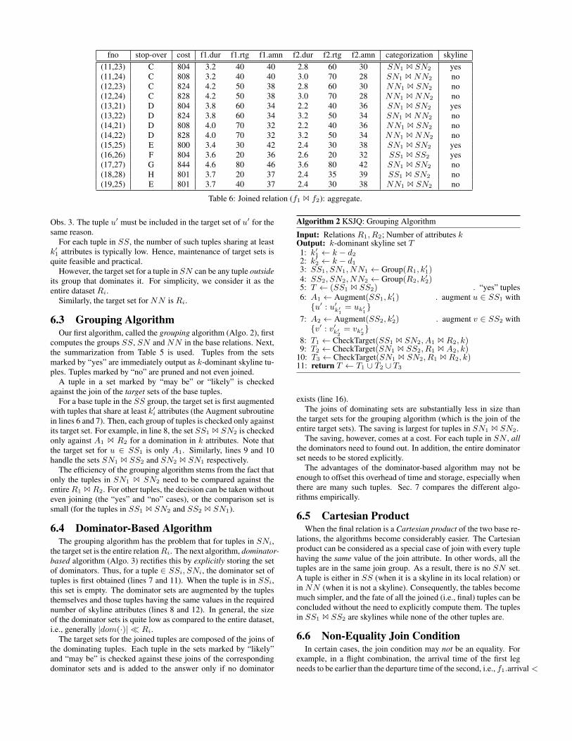
fno stop-over cost f1.dur f1.rtg f1.amn f2.dur f2.rtg f2.amn categorization skyline(11,23) C 804 3.2 40 40 2.8 60 30 SN1 1 SN2 yes(11,24) C 808 3.2 40 40 3.0 70 28 SN1 1 NN2 no(12,23) C 824 4.2 50 38 2.8 60 30 NN1 1 SN2 no(12,24) C 828 4.2 50 38 3.0 70 28 NN1 1 NN2 no(13,21) D 804 3.8 60 34 2.2 40 36 SN1 1 SN2 yes(13,22) D 824 3.8 60 34 3.2 50 34 SN1 1 NN2 no(14,21) D 808 4.0 70 32 2.2 40 36 NN1 1 SN2 no(14,22) D 828 4.0 70 32 3.2 50 34 NN1 1 NN2 no(15,25) E 800 3.4 30 42 2.4 30 38 SN1 1 SN2 yes(16,26) F 804 3.6 20 36 2.6 20 32 SS1 1 SS2 yes(17,27) G 844 4.6 80 46 3.6 80 42 SN1 1 SN2 no(18,28) H 801 3.7 20 37 2.4 35 39 SS1 1 SN2 no(19,25) E 801 3.7 40 37 2.4 30 38 NN1 1 SN2 no

Table 6: Joined relation (f1 1 f2): aggregate.

Obs. 3. The tuple u′ must be included in the target set of u′ for thesame reason.

For each tuple in SS, the number of such tuples sharing at leastk′1 attributes is typically low. Hence, maintenance of target sets isquite feasible and practical.

However, the target set for a tuple in SN can be any tuple outsideits group that dominates it. For simplicity, we consider it as theentire dataset Ri.

Similarly, the target set for NN is Ri.

6.3 Grouping AlgorithmOur first algorithm, called the grouping algorithm (Algo. 2), first

computes the groups SS, SN and NN in the base relations. Next,the summarization from Table 5 is used. Tuples from the setsmarked by “yes” are immediately output as k-dominant skyline tu-ples. Tuples marked by “no” are pruned and not even joined.

A tuple in a set marked by “may be” or “likely” is checkedagainst the join of the target sets of the base tuples.

For a base tuple in the SS group, the target set is first augmentedwith tuples that share at least k′i attributes (the Augment subroutinein lines 6 and 7). Then, each group of tuples is checked only againstits target set. For example, in line 8, the set SS1 1 SN2 is checkedonly against A1 1 R2 for a domination in k attributes. Note thatthe target set for u ∈ SS1 is only A1. Similarly, lines 9 and 10handle the sets SN1 1 SS2 and SN2 1 SN1 respectively.

The efficiency of the grouping algorithm stems from the fact thatonly the tuples in SN1 1 SN2 need to be compared against theentireR1 1 R2. For other tuples, the decision can be taken withouteven joining (the “yes” and “no” cases), or the comparison set issmall (for the tuples in SS1 1 SN2 and SS2 1 SN1).

6.4 Dominator-Based AlgorithmThe grouping algorithm has the problem that for tuples in SNi,

the target set is the entire relationRi. The next algorithm, dominator-based algorithm (Algo. 3) rectifies this by explicitly storing the setof dominators. Thus, for a tuple ∈ SSi, SNi, the dominator set oftuples is first obtained (lines 7 and 11). When the tuple is in SSi,this set is empty. The dominator sets are augmented by the tuplesthemselves and those tuples having the same values in the requirednumber of skyline attributes (lines 8 and 12). In general, the sizeof the dominator sets is quite low as compared to the entire dataset,i.e., generally |dom(·)| � Ri.

The target sets for the joined tuples are composed of the joins ofthe dominating tuples. Each tuple in the sets marked by “likely”and “may be” is checked against these joins of the correspondingdominator sets and is added to the answer only if no dominator

Algorithm 2 KSJQ: Grouping Algorithm

Input: Relations R1, R2; Number of attributes kOutput: k-dominant skyline set T1: k′1 ← k − d22: k′2 ← k − d13: SS1, SN1, NN1 ← Group(R1, k

′1)

4: SS2, SN2, NN2 ← Group(R2, k′2)

5: T ← (SS1 1 SS2) . “yes” tuples6: A1 ← Augment(SS1, k

′1) . augment u ∈ SS1 with

{u′ : u′k′1

= uk′1}

7: A2 ← Augment(SS2, k′2) . augment v ∈ SS2 with

{v′ : v′k′2

= vk′2}

8: T1 ← CheckTarget(SS1 1 SN2, A1 1 R2, k)9: T2 ← CheckTarget(SN1 1 SS2, R1 1 A2, k)

10: T3 ← CheckTarget(SN1 1 SN2, R1 1 R2, k)11: return T ← T1 ∪ T2 ∪ T3

exists (line 16).The joins of dominating sets are substantially less in size than

the target sets for the grouping algorithm (which is the join of theentire target sets). The saving is largest for tuples in SN1 1 SN2.

The saving, however, comes at a cost. For each tuple in SN , allthe dominators need to found out. In addition, the entire dominatorset needs to be stored explicitly.

The advantages of the dominator-based algorithm may not beenough to offset this overhead of time and storage, especially whenthere are many such tuples. Sec. 7 compares the different algo-rithms empirically.

6.5 Cartesian ProductWhen the final relation is a Cartesian product of the two base re-

lations, the algorithms become considerably easier. The Cartesianproduct can be considered as a special case of join with every tuplehaving the same value of the join attribute. In other words, all thetuples are in the same join group. As a result, there is no SN set.A tuple is either in SS (when it is a skyline in its local relation) orin NN (when it is not a skyline). Consequently, the tables becomemuch simpler, and the fate of all the joined (i.e., final) tuples can beconcluded without the need to explicitly compute them. The tuplesin SS1 1 SS2 are skylines while none of the other tuples are.

6.6 Non-Equality Join ConditionIn certain cases, the join condition may not be an equality. For

example, in a flight combination, the arrival time of the first legneeds to be earlier than the departure time of the second, i.e., f1.arrival <

Algorithm 3 KSJQ: Dominator-Based Algorithm

Input: Relations R1, R2; Number of attributes kOutput: k-dominant skyline set T1: k′1 ← k − d22: k′2 ← k − d13: SS1, SN1, NN1 ← Group(R1, k

′1)

4: SS2, SN2, NN2 ← Group(R2, k′2)

5: T ← (SS1 1 SS2) . “yes” tuples6: for each u ∈ SS1, SN1 do7: dom(u)← k′1-dominators(u) . dominators of u with k′1

attributes8: dom(u)← dom(u)∪ Augment(u, k′1) .{u′ : u′k′

1= uk′

1}

9: end for10: for each v ∈ SS2, SN2 do11: dom(v)← k′2-dominators(v) . dominators of v with k′2

attributes12: dom(v)← dom(v)∪ Augment(v, k′2) .{v′ : v′k′

2= vk′

2}

13: end for14: T ← ∅15: for each u 1 v ∈ (SS1 1 SN2) ∪ (SN1 1 SS2) ∪ (SN1 1

SN2) do16: T ← T∪ CheckDominators(dom(u) 1 dom(v), k)17: end for18: return T

f2.departure. In this section, we discuss how to handle such joincases when the condition is one of <,≤, >,≥.

Since the main purpose of dividing a base relation into the threesets SS, SN and NN is to ensure that certain decisions can betaken about the tuples in these sets without joining, all the optimiza-tions discussed in Sec. 5 work with the following modifications.

A tuple in SS1 1 SS2 can never be k-dominated and, thus, itdoes not matter how such a tuple is composed from the base rela-tions. In other words, the semantics of the join condition, equalityor otherwise, does not matter for SS1 1 SS2 tuples.

Next consider a tuple t′ = u′ 1 v′ ∈ (SN1 1 SS2). A tuple inthe SN set, u′, is originally defined as one that is not dominated byany other tuple in the same group. This ensures that if u′ joins withv′ from the other relation, then no other tuple u can join with v′ todominate t′. This is the crucial property that needs to be maintainedeven when the join condition is non-equality.

Thus, if the join condition is u′.arr < v′.dep, then the set {u :u.arr < u′.arr} is considered to be in the same group of u′ sinceit can also join with v′ (and can potentially dominate u). In otherwords, this ensures that all such u is join compatible with v′. Theset SN is thus expanded to take care of the non-equality condition.Note that there may exist other tuples {u′′ : u′′.arr < v′.dep} thatmay also join with v′; these, however, cannot be determined locallywithout the knowledge of v′ from the other relation and, therefore,cannot be considered. The target set of a tuple in SN is anyway theentire dataset (or its dominators). Thus, the algorithms will workcorrectly with the above modification.

Similarly, for the converse set, SS1 1 SN2, the SN set for v′

consists of {v : v.dep > v′.dep}.A joined tuple with NN as a component is rejected as a k-

dominant skyline since the NN tuple can be always dominated byanother tuple in the same group. Hence, similar to SN , the groupof a tuple needs to be defined by taking into account the semanticsof the join condition.

Considering the earlier example of u′.arr < v′.dep, if u′ ∈NN , then to say that u′ ∈ NN1, there must exist u : u.arr <u′.arr and u �k′

1u′. (The definition is suitably modified forNN2

Algorithm 4 Finding k: Naïve Algorithm

Input: Number of skylines δOutput: Number of attributes k1: k ← max{d1, d2}+ 1 . minimum k2: while k < d do3: if |skyline(k)| ≥ δ then . actual number4: return k . return and terminate5: end if6: k ← k + 17: end while8: return d . maximum possible k

in a suitable manner.) This ensures that the joined tuple t′ = u′ 1v′ will be dominated by u 1 v′. Once more, tuples of the form{u′′ : u′′.arr < v′.dep} are left out due to lack of knowledgeabout v′.

It may happen that there does not exist any such u but there existssuch an u′′. In that case, u′ is classified as an SN tuple insteadof an NN . This, however, only leads to extra processing of tuplesjoined with u′. The correctness is not violated as such joined tuplesof the form t′ = u′ 1 v′ will be finally caught by u′′ 1 v′ andrejected. Thus, the above modification only affects the efficiencyof the algorithms, not the final result.

6.7 Algorithms for AggregationThe algorithms that consider aggregation are essentially the same

as the plain KSJQ. The only difference is that when the join is per-formed, the aggregation of the attributes are done as an additionalstep. Therefore, they are not discussed separately.

We next discuss the algorithms for finding k (Problem 3).

6.8 Finding k: Naïve AlgorithmThe naïve algorithm (Algo. 4) to search for the lowest k that

produces at least δ skylines starts from the least possible value ofk, i.e., max{d1, d2}+ 1, and keeps incrementing it till the numberof k-dominant skylines is at least δ. The largest possible value ofk, i.e., d, is otherwise returned by default, even if it does not satisfythe δ criterion.

The algorithm is very inefficient as for each case, it computes theactual k-dominant skyline set. Further, it traverses the possibilitiesof k in a linear manner. The correctness is based on the fact that thenumber of k-dominant skylines is a monotonically non-decreasingfunction in k (Lemma 1).

We next design algorithms that use Table 5.

6.9 Finding k: Range-Based AlgorithmFor a particular value of k, the actual number of k-dominant sky-

lines, ∆k, is at least the size of the “yes” sets, denoted by ∆k,lb,and at most the sum of sizes of the “yes”, “likely” and “may be”sets, denoted by ∆k,ub. These, thus, denote the lower and upperbounds respectively: ∆k,lb < ∆k < ∆k,ub.

The range-based algorithm (Algo. 5) uses these bounds to speed-up the process. Starting from the minimum possible k = max{d1, d2}+1, the algorithm finds ∆k,lb and ∆k,ub (lines 3 and 4 respectively).If ∆k,lb ≥ δ, then the current k is the answer (line 5). If ∆k,ub <δ, then the current k cannot be the answer and k is incremented(line 7). Otherwise, i.e., if ∆k,lb < δ ≤ ∆k,ub, then the current kmay be an answer. In this case, the actual k-dominant skyline setis computed. If its size is δ or greater, it is returned as the answer(line 9). Else, k is incremented (line 11), and the steps are repeated.

While this algorithm is definitely more efficient than the naïveone, it still suffers from the shortcoming that it examines a largenumber of k’s by incrementing it one by one. If the required k lies

Algorithm 5 Finding k: Range-Based Algorithm

Input: Number of skylines δOutput: Number of attributes k1: k ← max{d1, d2}+ 1 . minimum k2: while k < d do3: ∆k,lb ← |“yes” sets|4: ∆k,ub ← |“yes” sets|+ |“likely” sets|+ |“may be” sets|5: if ∆k,lb ≥ δ then . lower bound6: return k7: else if ∆k,ub < δ then . upper bound8: k ← k + 19: else if |skyline(k)| ≥ δ then . actual number

10: return k11: else12: k ← k + 113: end if14: end while15: return d . maximum possible k

towards the higher end of the range, it unnecessarily examines toomany lower values of k. The next algorithm does a binary searchto reduce this overhead.

6.10 Finding k: Binary Search AlgorithmAlgo. 6 shows how the binary search proceeds. It starts from the

middle of the possible values of k (line 5). The values of ∆k,lb and∆k,ub are computed in the same manner as earlier (lines 6 and 7respectively).

If ∆k,lb ≥ δ (line 8), then k is a potential answer. No value inthe higher range can be the answer as the current k already satisfiesthe condition. However, there may be a lower k that satisfies the δcondition. Hence, the search is continued in the lower range to tryand find a better (i.e., lesser) k.

If, on the other hand, ∆k,ub < δ (line 11), then the current es-timate of k is too low. The search is, therefore, continued in thehigher range.

If none of these bounds help, the actual number of k-dominantskylines, ∆k, is found. If ∆k ≥ δ (line 13), then the current k isa potential answer. However, a lesser k may be found and, so, thesearch proceeds to the lower range.

Otherwise, i.e., when ∆k < δ (line 16), the required k is searchedin the higher range.

The algorithm stops when the lower range of the search becomeslarger than or equal to the current answer (line 19), which then isthe lowest k that satisfies the δ condition. It may also stop when therange is exhausted, in which case, the current value of k is returned(line 23).

The binary search based algorithm, thus, speeds up the searchingthrough the possible range of values of k. Sec. 7 compares the threealgorithms empirically.

7. EXPERIMENTAL RESULTSWe experimented with data synthetically generated using http://

randdataset.projects.pgfoundry.org/ on an Intel i7-4770 @3.40 GHzOctacore machine with 16 GB RAM using code written in Java.

We also experimented with a real dataset of two-legged flightsfrom New Delhi to Mumbai. The details are in Sec. 7.4.

We measured the effects of various parameters on the differentalgorithms proposed in Sec. 6. The parameters and their defaultvalues are listed in Table 7. Note that the size of the joined relationis a derived parameter. It is equal to n2/g for two base relationswith n tuples and g groups. When the effect of a particular set ofparameters are measured, the rest are held to their default values,

Algorithm 6 Finding k: Binary Search Algorithm

Input: Number of skylines δOutput: Number of attributes k1: l← max{d1, d2}+ 1 . minimum k2: h← d . maximum k3: cur ← d . current estimate of k4: while l < h do5: k ← b(l + h)/2c6: ∆k,lb ← |“yes” sets|7: ∆k,ub ← |“yes” sets|+ |“likely” sets|+ |“may be” sets|8: if ∆k,lb ≥ δ then9: cur ← k . update current estimate

10: h← k − 1 . search for a lower k11: else if ∆k,ub < δ then12: l← k + 1 . search for a higher k13: else if |skyline(k)| ≥ δ then14: cur ← k . update current estimate15: h← k − 1 . search for a lower k16: else if |skyline(k)| < δ then17: l← k + 1 . search for a higher k18: end if19: if l ≥ cur then . lowest k already found20: return cur21: end if22: end while23: return cur

Symbol Parameter Default valuen Dataset size for base relation 3, 300d Dimensionality of base relation 7k Number of skyline attributes 11a Number of aggregate attributes 2g Number of join groups 10T Dataset type Independentδ Threshold of skyline size 10, 000N Size of joined relation 1, 089, 000

Table 7: Parameters for experiments.

unless explicitly stated otherwise.In the figures, the three main algorithms for KSJQ are denoted

as: G for grouping, D for dominator-based, and N for naïve. Theoverall running time for each algorithm is divided into various com-ponents: (i) time taken for computing the groups in the base rela-tions, i.e., SS, SN , andNN , (ii) time taken for actually joining thetuples from the two base relations that cannot be pruned, (iii) timetaken for finding the dominators of the tuples, and (iv) the rest ofthe processing. These are marked separately in the figures.

Not all the components are applicable to every algorithm, e.g.,the naïve algorithm does not find groups. The components that arenot applicable to an algorithm are shown to have zero costs.

The three algorithms for determining the value of k are depictedas: B for binary search, R for range-based, and N for naïve.

7.1 AggregateWe first show the results where aggregate values have been used.

The aggregation function used is sum.

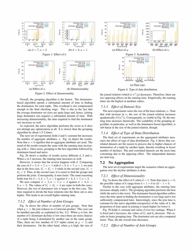
7.1.1 Effect of DimensionalityThe first experiment measures the effect of varying k. Fig. 1

shows that the running time increases sharply with k. The twodifferent settings of dimensionality, d, and number of aggregateattributes, a, (Fig. 1a and Fig. 1b) show the robustness of this be-havior. As k increases, it becomes increasingly hard to dominate atuple in k dimensions. As a result, the number of k-dominant sky-line increases heavily, thereby resulting in increased running times.

0

2

4

6

8

10

12

14

G D N G D N G D N G D N

Tim

e (

s)

k (d=7, a=2)

Grouping TimeJoin Time

Dominator GenerationRemaining

111098

0 0.5

1 1.5

2 2.5

1098

(a) d = 7, a = 2

0

1

2

3

4

5

6

7

8

G D N G D N G D N G D N

Tim

e (

s)

k (d=6, a=1)

Grouping TimeJoin Time

Dominator GenerationRemaining

10987

0 0.05

0.1 0.15

0.2 0.25

0.3 0.35

0.4

87

(b) d = 6, a = 1

Figure 1: Effect of k.

0

10

20

30

40

50

G D N G D N G D N G D N

Tim

e (

s)

a (d=7,k=11)

Grouping TimeJoin Time

Dominator GenerationRemaining

3210

(a) Effect of a.

0

0.2

0.4

0.6

0.8

1

1.2

1.4

1.6

GDN GDN GDN GDN GDN

Tim

e (

s)

d,k,a

Grouping TimeJoin Time

Dominator GenerationRemaining

6,8,26,7,26,7,15,7,25,7,1

(b) Dimensionality.

Figure 2: Effect of dimensionality.

Overall, the grouping algorithm is the fastest. The dominator-based algorithm spends a substantial amount of time in findingthe dominators for each tuple. This overhead is not compensatedenough in the final checking stage. This is due to the fact thatthe average dominator set sizes are quite large and, hence, joininglarge dominator sets requires a substantial amount of time. Withincreasing dimensionality, the time required to find the dominatorsets increases as well.

As expected, the naïve algorithm performs the worst as it doesnot attempt any optimization at all. It is slower than the groupingalgorithm by about 1.5-2 times.

The next set of experiments hold d and k constant but increasesthe number of aggregate attributes, a. Fig. 2a depict the results.Note that a = 0 signifies that no aggregate attributes are used. Thetrend of the results remain the same with the running time increas-ing with a. Once more, grouping is the best algorithm followed bydominator-based and naïve.

Fig. 2b shows a medley of results across different d, k and a.When a or k increase, the running time increases as well.

However, it seems that the reverse happens with d. Comparingthe case of d = 5, k = 7, a = 1 with d = 6, k = 7, a = 1, we notethat in the first case, k′1 = k′2 = 3 while in the second case, k′1 =k′2 = 2. Thus, in the second case, it is easier to find the groups andperform the joins. Consequently, it runs faster. The same reasoningholds true for d = 5, k = 7, a = 2 against d = 6, k = 7, a = 2.

We next compare d = 5, k = 7, a = 2 against d = 6, k =8, a = 2. The values of k′1 = k′2 = 4 are same in both the cases.However, the size of dominator sets is larger in the first case. Thetime required to divide the base relations into the three sets is alsohigher. This leads to an overall higher running time.

7.1.2 Effect of Number of Join GroupsFig. 3a shows the effect of number of join groups. Note that

when g = 1, the join reduces to a Cartesian product. This case canbe handled specially as explained in Sec. 6.5. When g is low, thenumber of k-dominant skylines is low since there are more chancesof a tuple being k-dominated by another one in the same group.Thus, there are less number of SN tuples (none at g = 1) andtheir dominators. On the other hand, when g is high, the size of

0

10

20

30

40

50

60

GDN GDN GDN GDN GDN GDN GDN

Tim

e (

s)

Group Size (g)

Grouping TimeJoin Time

Dominator GenerationRemaining

100502510521

(a) Effect of g.

0

200

400

600

800

1000

1200

1400

GDN GDN GDN GDN GDN GDN

Tim

e (

s)

Dataset size (n)

Grouping TimeJoin Time

Dominator GenerationRemaining

33K10K3.3K1K330100

0

1 2

3 4

5

1K330100

(b) Effect of n.

Figure 3: Scalability.

0

10

20

30

40

50

G D N G D N G D N

Tim

e (

s)

Data Type

Grouping TimeJoin Time

Dominator GenerationRemaining

Anti-CorrelatedCorrelatedIndependent

(a) Data type.

Figure 4: Type of data distribution.

the joined relation (which is n2/g) decreases. Therefore, there aretwo opposing effects on the running time. Empirically, the runningtimes are the highest at medium values.

7.1.3 Effect of Dataset SizeThe next experiment varies the size of the base relations, n. Note

that with increase in n, the size of the joined relation increasesquadratically (O(n2)). Consequently, as visible in Fig. 3b, the run-ning time increases drastically. The scalability of the grouping al-gorithm, in particular, as well as the dominator-based algorithm, issub-linear in the size of the joined relation, though.

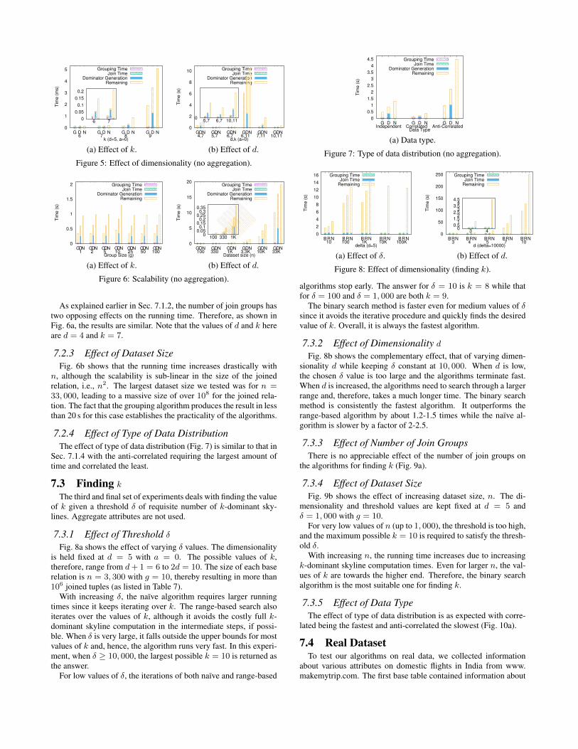
7.1.4 Effect of Type of Data DistributionThe final set of experiments on the aggregated attributes mea-

sures the effect of type of data distribution. Fig. 4 shows that cor-related datasets are the easiest to process due to higher chances ofdomination of a tuple by another tuple, thereby resulting in lessernumber of skylines. The anti-correlated datasets are the most timeconsuming due to the opposing effect. The independent datasetsare mid-way.

7.2 No AggregationThe next set of experiments target the scenarios where no aggre-

gation over the skyline attributes is done.

7.2.1 Effect of DimensionalityFig. 5a shows the effect of k when d = 5. Note that since a = 0,

the possible values of k range from d+ 1 = 6 to 2d− 1 = 9.Similar to the case with aggregate attributes, the running time

increases sharply with k. The grouping algorithm performs the bestwhile the naïve is the worst. The dominator-based algorithm sufferssince the time spent in finding the dominators is too large and is notsufficiently compensated later. Interestingly, since the join time isconstant for the naïve algorithm irrespective of the value of k, theproportion of time spent in joining is much higher for lower k.

Fig. 5b holds k constant and varies d over two settings. When kis fixed and d increases, the values of k′1 and k′2 decrease. This re-sults in faster grouping time. The dominator sets are also computedfaster. Thus, the the overall time decreases.

7.2.2 Effect of Number of Join Groups

0

1

2

3

4

5

G D N G D N G D N G D N

Tim

e (

ms)

k (d=5, a=0)

Grouping TimeJoin Time

Dominator GenerationRemaining

9876

0

0.05

0.1

0.15

0.2

76

(a) Effect of k.

0

2

4

6

8

10

GDN GDN GDN GDN GDN GDN

Tim

e (

s)

d,k (a=0)

Grouping TimeJoin Time

Dominator GenerationRemaining

10,117,116,116,75,74,7

010,116,75,7

(b) Effect of d.

Figure 5: Effect of dimensionality (no aggregation).

0

0.5

1

1.5

2

GDN GDN GDN GDN GDN GDN GDN

Tim

e (

s)

Group Size (g)

Grouping TimeJoin Time

Dominator GenerationRemaining

100502510521

(a) Effect of k.

0

5

10

15

20

GDN GDN GDN GDN GDN GDN

Tim

e (

s)

Dataset size (n)

Grouping TimeJoin Time

Dominator GenerationRemaining

33K10K3.3K1K330100

0 0.05

0.1 0.15

0.2 0.25

0.3 0.35

1K330100

(b) Effect of d.

Figure 6: Scalability (no aggregation).

As explained earlier in Sec. 7.1.2, the number of join groups hastwo opposing effects on the running time. Therefore, as shown inFig. 6a, the results are similar. Note that the values of d and k hereare d = 4 and k = 7.

7.2.3 Effect of Dataset SizeFig. 6b shows that the running time increases drastically with

n, although the scalability is sub-linear in the size of the joinedrelation, i.e., n2. The largest dataset size we tested was for n =33, 000, leading to a massive size of over 108 for the joined rela-tion. The fact that the grouping algorithm produces the result in lessthan 20 s for this case establishes the practicality of the algorithms.

7.2.4 Effect of Type of Data DistributionThe effect of type of data distribution (Fig. 7) is similar to that in

Sec. 7.1.4 with the anti-correlated requiring the largest amount oftime and correlated the least.

7.3 Finding k

The third and final set of experiments deals with finding the valueof k given a threshold δ of requisite number of k-dominant sky-lines. Aggregate attributes are not used.

7.3.1 Effect of Threshold δ

Fig. 8a shows the effect of varying δ values. The dimensionalityis held fixed at d = 5 with a = 0. The possible values of k,therefore, range from d+ 1 = 6 to 2d = 10. The size of each baserelation is n = 3, 300 with g = 10, thereby resulting in more than106 joined tuples (as listed in Table 7).

With increasing δ, the naïve algorithm requires larger runningtimes since it keeps iterating over k. The range-based search alsoiterates over the values of k, although it avoids the costly full k-dominant skyline computation in the intermediate steps, if possi-ble. When δ is very large, it falls outside the upper bounds for mostvalues of k and, hence, the algorithm runs very fast. In this experi-ment, when δ ≥ 10, 000, the largest possible k = 10 is returned asthe answer.

For low values of δ, the iterations of both naïve and range-based

0

0.5

1

1.5

2

2.5

3

3.5

4

4.5

G D N G D N G D N

Tim

e (

s)

Data Type

Grouping TimeJoin Time

Dominator GenerationRemaining

Anti-CorrelatedCorrelatedIndependent

(a) Data type.

Figure 7: Type of data distribution (no aggregation).

0

2

4

6

8

10

12

14

16

BRN BRN BRN BRN BRN

Tim

e (

s)

delta (d=5)

Grouping TimeJoin Time

Remaining

100K10K1K10010

(a) Effect of δ.

0

50

100

150

200

250

BRN BRN BRN BRN BRN

Tim

e (

s)

d (delta=10000)

Grouping TimeJoin Time

Remaining

107543

0 0.5

1 1.5

2 2.5

3 3.5

4 4.5

43

(b) Effect of d.

Figure 8: Effect of dimensionality (finding k).

algorithms stop early. The answer for δ = 10 is k = 8 while thatfor δ = 100 and δ = 1, 000 are both k = 9.

The binary search method is faster even for medium values of δsince it avoids the iterative procedure and quickly finds the desiredvalue of k. Overall, it is always the fastest algorithm.

7.3.2 Effect of Dimensionality dFig. 8b shows the complementary effect, that of varying dimen-

sionality d while keeping δ constant at 10, 000. When d is low,the chosen δ value is too large and the algorithms terminate fast.When d is increased, the algorithms need to search through a largerrange and, therefore, takes a much longer time. The binary searchmethod is consistently the fastest algorithm. It outperforms therange-based algorithm by about 1.2-1.5 times while the naïve al-gorithm is slower by a factor of 2-2.5.

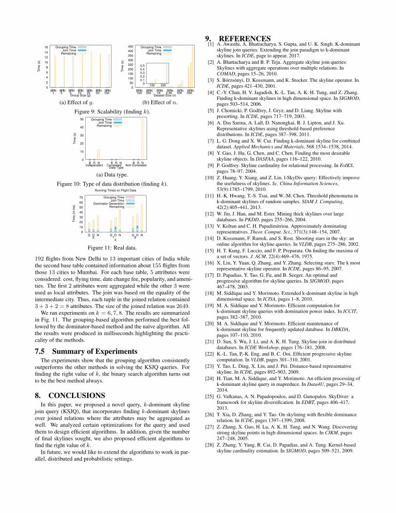
7.3.3 Effect of Number of Join GroupsThere is no appreciable effect of the number of join groups on

the algorithms for finding k (Fig. 9a).

7.3.4 Effect of Dataset SizeFig. 9b shows the effect of increasing dataset size, n. The di-

mensionality and threshold values are kept fixed at d = 5 andδ = 1, 000 with g = 10.

For very low values of n (up to 1, 000), the threshold is too high,and the maximum possible k = 10 is required to satisfy the thresh-old δ.

With increasing n, the running time increases due to increasingk-dominant skyline computation times. Even for larger n, the val-ues of k are towards the higher end. Therefore, the binary searchalgorithm is the most suitable one for finding k.

7.3.5 Effect of Data TypeThe effect of type of data distribution is as expected with corre-

lated being the fastest and anti-correlated the slowest (Fig. 10a).

7.4 Real DatasetTo test our algorithms on real data, we collected information

about various attributes on domestic flights in India from www.makemytrip.com. The first base table contained information about

0

2

4

6

8

10

12

14

16

BRN BRN BRN BRN BRN BRN BRN

Tim

e (

s)

Group Size (g)

Grouping TimeJoin Time

Remaining

100502510521

(a) Effect of g.

0

50

100

150

200

250

300

350

400

450

BRN BRN BRN BRN BRN BRN

Tim

e (

s)

Dataset Size (n)

Grouping TimeJoin Time

Remaining

33K10K3.3K1K330100

0 0.1 0.2 0.3 0.4 0.5

330100

(b) Effect of n.

Figure 9: Scalability (finding k).

0

10

20

30

40

50

B R N B R N B R N

Tim

e (

s)

Data Type

Grouping TimeJoin Time

Remaining

Anti-CorrelatedCorrelatedIndependent

(a) Data type.

Figure 10: Type of data distribution (finding k).

0

10

20

30

40

50

60

70

G D N G D N G D N

Tim

e (

in m

s)

k

Running Times on Flight Data

Grouping TimeJoin Time

Dominator GenerationRemaining

876

Figure 11: Real data.

192 flights from New Delhi to 13 important cities of India whilethe second base table contained information about 155 flights fromthose 13 cities to Mumbai. For each base table, 5 attributes wereconsidered: cost, flying time, date change fee, popularity, and ameni-ties. The first 2 attributes were aggregated while the other 3 wereused as local attributes. The join was based on the equality of theintermediate city. Thus, each tuple in the joined relation contained3 + 3 + 2 = 8 attributes. The size of the joined relation was 2649.

We ran experiments on k = 6, 7, 8. The results are summarizedin Fig. 11. The grouping-based algorithm performed the best fol-lowed by the dominator-based method and the naïve algorithm. Allthe results were produced in milliseconds highlighting the practi-cality of the methods.

7.5 Summary of ExperimentsThe experiments show that the grouping algorithm consistently

outperforms the other methods in solving the KSJQ queries. Forfinding the right value of k, the binary search algorithm turns outto be the best method always.

8. CONCLUSIONSIn this paper, we proposed a novel query, k-dominant skyline

join query (KSJQ), that incorporates finding k-dominant skylinesover joined relations where the attributes may be aggregated aswell. We analyzed certain optimizations for the query and usedthem to design efficient algorithms. In addition, given the numberof final skylines sought, we also proposed efficient algorithms tofind the right value of k.

In future, we would like to extend the algorithms to work in par-allel, distributed and probabilistic settings.

9. REFERENCES[1] A. Awasthi, A. Bhattacharya, S. Gupta, and U. K. Singh. K-dominant

skyline join queries: Extending the join paradigm to k-dominantskylines. In ICDE, page to appear, 2017.

[2] A. Bhattacharya and B. P. Teja. Aggregate skyline join queries:Skylines with aggregate operations over multiple relations. InCOMAD, pages 15–26, 2010.

[3] S. Börzsönyi, D. Kossmann, and K. Stocker. The skyline operator. InICDE, pages 421–430, 2001.

[4] C.-Y. Chan, H. V. Jagadish, K.-L. Tan, A. K. H. Tung, and Z. Zhang.Finding k-dominant skylines in high dimensional space. In SIGMOD,pages 503–514, 2006.

[5] J. Chomicki, P. Godfrey, J. Gryz, and D. Liang. Skyline withpresorting. In ICDE, pages 717–719, 2003.

[6] A. Das Sarma, A. Lall, D. Nanongkai, R. J. Lipton, and J. Xu.Representative skylines using threshold-based preferencedistributions. In ICDE, pages 387–398, 2011.

[7] L. G. Dong and X. W. Cui. Finding k-dominant skyline for combineddataset. Applied Mechanics and Materials, 568:1534–1538, 2014.

[8] Y. Gao, J. Hu, G. Chen, and C. Chen. Finding the most desirableskyline objects. In DASFAA, pages 116–122, 2010.

[9] P. Godfrey. Skyline cardinality for relational processing. In FoIKS,pages 78–97, 2004.

[10] Z. Huang, Y. Xiang, and Z. Lin. l-SkyDiv query: Effectively improvethe usefulness of skylines. Sc. China Information Sciences,53(9):1785–1799, 2010.

[11] H.-K. Hwang, T.-S. Tsai, and W.-M. Chen. Threshold phenomena ink-dominant skylines of random samples. SIAM J. Computing,42(2):405–441, 2013.

[12] W. Jin, J. Han, and M. Ester. Mining thick skylines over largedatabases. In PKDD, pages 255–266, 2004.

[13] V. Koltun and C. H. Papadimitriou. Approximately dominatingrepresentatives. Theor. Comput. Sci., 371(3):148–154, 2007.

[14] D. Kossmann, F. Ramsk, and S. Rost. Shooting stars in the sky: anonline algorithm for skyline queries. In VLDB, pages 275–286, 2002.

[15] H. T. Kung, F. Luccio, and F. P. Preparata. On finding the maxima ofa set of vectors. J. ACM, 22(4):469–476, 1975.

[16] X. Lin, Y. Yuan, Q. Zhang, and Y. Zhang. Selecting stars: The k mostrepresentative skyline operator. In ICDE, pages 86–95, 2007.

[17] D. Papadias, Y. Tao, G. Fu, and B. Seeger. An optimal andprogressive algorithm for skyline queries. In SIGMOD, pages467–478, 2003.

[18] M. Siddique and Y. Morimoto. Extended k-dominant skyline in highdimensional space. In ICISA, pages 1–8, 2010.

[19] M. A. Siddique and Y. Morimoto. Efficient computation fork-dominant skyline queries with domination power index. In ICCIT,pages 382–387, 2010.

[20] M. A. Siddique and Y. Morimoto. Efficient maintenance ofk-dominant skyline for frequently updated database. In DBKDA,pages 107–110, 2010.

[21] D. Sun, S. Wu, J. Li, and A. K. H. Tung. Skyline-join in distributeddatabases. In ICDE Workshop, pages 176–181, 2008.

[22] K.-L. Tan, P.-K. Eng, and B. C. Ooi. Efficient progressive skylinecomputation. In VLDB, pages 301–310, 2001.

[23] Y. Tao, L. Ding, X. Lin, and J. Pei. Distance-based representativeskyline. In ICDE, pages 892–903, 2009.

[24] H. Tian, M. A. Siddique, and Y. Morimoto. An efficient processing ofk-dominant skyline query in mapreduce. In Data4U, pages 29–34,2014.

[25] G. Valkanas, A. N. Papadopoulos, and D. Gunopulos. SkyDiver: aframework for skyline diversification. In EDBT, pages 406–417,2013.

[26] T. Xia, D. Zhang, and Y. Tao. On skylining with flexible dominancerelation. In ICDE, pages 1397–1399, 2008.

[27] Z. Zhang, X. Guo, H. Lu, A. K. H. Tung, and N. Wang. Discoveringstrong skyline points in high dimensional spaces. In CIKM, pages247–248, 2005.

[28] Z. Zhang, Y. Yang, R. Cai, D. Papadias, and A. Tung. Kernel-basedskyline cardinality estimation. In SIGMOD, pages 509–521, 2009.