k Development Team - epgp.inflibnet.ac.in

ZOOLOGY Principles of Ecology

Life table, Fecundity table and Survivorship curves, Part-I

1

k

Paper : 12 Principles of Ecology

Module : 08a Life Table, Fecundity Table and Survivorship curves, Part-I

Development Team

Paper Coordinator: Prof. D.K. Singh Department of Zoology, University of Delhi

Principal Investigator: Prof. Neeta Sehgal Department of Zoology, University of Delhi

Content Writer: Dr. Kapinder and Dr. Haren Ram Chiary Kirori Mal College, University of Delhi

Content Reviewer: Prof. K.S. Rao Department of Botany, University of Delhi

Co-Principal Investigator: Prof. D.K. Singh Department of Zoology, University of Delhi



2

Description of Module

Subject Name ZOOLOGY

Paper Name Zool 12 Principles of Ecology

Module Name/Title Population

Module Id M08a: Life Table, Fecundity Table and Survivorship curves,

Part-I

Keywords Life table, horizontal life table, vertical life table, composite

life table,

Content:

1. Learning Outcomes

2. Introduction

3. Semelparous vs iteroparous life cycles

4. Life tables

5. Types of life tables

5.1. Horizontal life table

5.2. Vertical life table

5.3. Dynamic composite life table

6. Components of a life table

7. Construction of cohort life table

8. Construction of static life table

9. Application of life table

10. Summary



3

1. Learning Outcomes

After studying this module, you shall be able to:

Understand quantitative aspect of population ecology.

Understand different parameters that derive population change.

Know different types of life table.

Construct life table of different animals.

2. Introduction

A population can be defined as a localized group of individuals belonging to the same

species. Sometimes, few populations shows distinct boundaries like population of White-

footed Mouse in Sandford Natural Area, however, in other cases, population did not have

demarcated boundaries, therefore it is randomly set by the convenience of the investigators,

for instance, Eastern Chipmunks around Holmes Hall. The next step after defining the

boundaries is the determination of a population size. It can be done by either counting total

number of individuals from a given smaller sample area which can be extrapolated to the set

boundaries or it can be done by capture-recapture method.

The population biology is mainly concerned with the factors which can alter the population

size with time. The important factors are mainly natality, mortality, growth of individual and

reproductive success. The strength of population ecology lies in its quantitative nature. For

example, what will happens if survival rate of Bald eagle is decreased by 2% per year? Or if

survival of juvenile salmon is increased by 0.5%, how many adult salmons would reach to

their maturity? These simple questions can be answered by applying simple mathematics in

the population ecology. In this module we will understand the quantitative background for

population ecology.



4

3. Semelparous vs Iteroparous life cycles

Some species (e.g., most invertebrates) in their life time have only one reproductive event

and after that they die. The efforts of these species in the reproductive events spend enormous

energy in order to produce large number of eggs, whereas, other species (e.g., most birds and

mammals) live to perform several reproductive events in their lives. There is a great amount

of variation in these two categories. For instance, some species of semelparous organisms

have overlapping generations of young ones, as a result, there may be one year or two year

old individuals can be found in the population. The common form of semelparity found in the

insects living in temperate regions is an annual species. In these conditions, the insect survive

as an egg or larval resting stage during overwinters until spring and after that in the summer

months they grows and matures into the adult which perform reproductive events. After

mating, these adults lay eggs which survive in the same dormant stage in adverse condition

throughout the winter months. However, several other semelparous species can produce

several generations each season of summer. It is now easy to understand that importance of

reproductive event frequencies, the young ones produced in each reproductive event and

generation time that can greatly influence how fast a population can grow.

4. Life tables

Mortality is one of the important parameters that derive changes in the population. There are

several kinds of questions such as, is mortality more among young organism? Does an old

aged individual have higher mortality than younger organism? We can answer these kinds

of questions by constructing a life table. Life table was build up by those human

demographers who were working for life insurance companies and were interested to

estimate the life expectancy of the people. Plants and animal populations may be composed

of several types of individuals and in any given analysis a demographer may group them

together or may keep them separate.



5

A life table can be explained as an age specific summary of mortality rates that is operating

on a cohort of individuals. A cohort may consist of either the entire population or it may

include only the males or females individuals that were born in a given period of time.

The life table is most frequently used by the life insurance companies to find out the

probability of survivorships of human populations for deciding the premium whereas,

ecologists uses life table to study the natural populations. Raymond Pearl, (1921) (figure 1)

first used life table for the population of Drosophila reared in the laboratory.

Figure.1: Raymond Pearl

Generally, it is very difficult to construct life tables of non-human populations living in the

wild conditions. The life table construction is a very simple method to keep track of birth

rate, death rate and reproductive events in the given population. The following types of data

can be used to construct the ecological life table.

Laboratory animals: The life tables of these animals of known age can be constructed by

directly observing the individuals which are dying at regular intervals and the observation

will be continued till all individuals in a population died.

Survivorship directly observed: The survival of large cohort can be studies by following

at regular intervals till their existence. Connell (1961) studied mortality of the barnacle



6

Chthamalus stellatus, grew on the rocks during autumn season in Scotland. The mortality

of these barnacles was observed at regular interval and the data was used to construct the

life table. He did several experiments in which he removed one competing barnacle

Balanus balanoides from some rocks and then he counted the number of Chthamalus

surviving once in a month.

Age structure directly observed: This type of data can be used to construct the static life

table, particularly of trees, birds, fishes and many more. The information regarding age

structure can be acquired by observing the annular rings in the horns of sheep, growth

rings in the cementum of teeth in case of ungulates as well as carnivores and annular rings

present on the fish scales. For example, in a pond, we can get a sample of fish which can

be used to determine the age of each fish simply by analyzing the number of the annular

rings present on their scales. Similarly, age of the tree can be determined by counting the

tree rings. However, these types of data are not always preferred for making life tables.

Age at death: This type of data can be used to construct the static life table. We assume

that population size is constant over time and birth rate, death rate of population at each

age interval remains constant. Sinclair (1977) constructs the life table of African buffalo

(Syncerus caffer) by collecting 584 skulls that died due to natural causes. After that he

classified these skulls on the basis of sex and age. The age of the skull was determined by

analyzing the annular rings on the horns. The estimation of age of young skull was

difficult because they were fragile and more susceptible to carnivores and damage by

environment. He observed the losses in first two year of life by directly observing the herd

and obtained the mortality data.

5. Types of Life tables

The life tables for human populations can be formed by analyzing the data of birth and death

recorded by municipal committees of different states as well as by life insurance companies.

Life tables can be classified into following three types:



7

5.1 Horizontal life table

It is also known as cohort or dynamic life table. This type of life table is constructed by

observing the survival and reproduction of all individuals of a cohort from the time of birth to

the death of all members of the population. A cohort is considered as the group of all

individuals born or recruited into a population during given period of time. For example, a

cohort can be start with one thousand individuals and observation of number of dying

individuals can be done at regular intervals till all the individuals in a population is

exhausted. It is usually related to those species which have short life span and their

generations are discrete.

5.2 Vertical life table

It is also considered as time specific life table or static life table. The vertical life table can be

constructed by recording the total number of individuals surviving at each age group in a

given population and their reproductive output. This life table is based on the assumption that

each age class is sampled in proportion to its numbers in a population. It also assumes that

the population is stable and death rates and birth rates in a population are constant.

5.3 Dynamic composite life table

The construction of this type of life table is similar as cohort life table; however, in this case,

the cohort is a composite of a number of individuals that are marked over a period of years

rather than at the time of birth only.

The dynamic composite life table and static life tables are considered as less accurate

whereas, cohort life table provides a reasonable idea about average conditions of the

populations. The life tables are very useful in comparing the trends of life history within a

population and also in between different populations.

The cohort or static life tables which classify individuals of a population by age groups are

called as age based life tables. In these types of life tables, individuals who survived for less

than one year are assigned zero age and those individuals in a population which lived for one

or more year but less than two years are allotted one year age and so on. However, size-based

life tables and stage-based life tables usually classify individuals by their size or stage of

developmental instead of age. Generally, these types of life tables are more useful and more



8

practical for understanding those organisms which cannot be differentiated by their age as

well as their ecological roles are chiefly depends on their size or stage rather than age.

6. Components of a life table

1. First column x in the life table provides age intervals of the individuals in time units

suitable according to the species.

2. Second column nx gives number of individuals surviving at that particular age interval.

3. Third column lx gives proportion surviving. It can start with one thousand individuals that

enter in the first age group and gives the remaining number at the beginning of each

subsequent age interval. It is calculated by the formula:

lx = lx1/nx1 X nx2

4. Fourth column dx represents number of individuals dying at each age interval from the

initial group of 1000 individuals. It is calculated by:

dx = lx – l(x+1)

5. Fifth column ex denotes life expectancy. It determines the total expected survival of an

individual of a given age beyond its present age. It can be calculated by following three steps;

a) Lx is average number of individuals alive. Calculate the proportion of survivors at

the mid-point of each time interval.

Lx = lx + l(x+1)/2

b). Tx is total life time remaining for all the individuals attaining the age. Sum all the Lx

values from the age of interest upto the oldest age:

Tx = Σ Lx

c) ex = Tx/lx



9

7. Construction of cohort life table

To construct a cohort life table, for example, individuals born in the United States during the

year 1900, the survival of these individuals were recorded from the beginning of 1901, 1902,

1903, 1904 and so on until all individuals were die. This record is called the survivorship

schedule.

Mostly, life tables calculate only females and their female offspring for those animals in

which there are males and females and both of them are equal in numbers of each age. Most

plants, hermaphrodite animals and other organisms in which there is no sexual dimorphism,

life table calculations may have to be adjusted.

The construction of life table for this simple life history can be done by counting the

population size at each life stage. The first column (x) denotes the age class and second

column (nx) specify the number of individuals survived at the beginning of each age. These

data can be used to calculate several other life history parameters, such as the proportion

surviving at each life stage (lx), proportion of individuals dying at each age (dx) and age-

specific mortality rate (qx) dying at each age which is helpful in locating the points where

mortality is most intense.

Example.1: Cohort life table of song sparrow on Mandarte Island, British Columbia

(Source: Smith 1988).

Age in yrs

(x)

Observed No.

birds alive each

year (nx)

Proportion

surviving at

Start of Age

Interval x (lx)

No. dying

within Age

interval x to

x + 1 (dx)

Rate of

mortality (qx)

0 115 1.0 90 0.78

1 25 0.217 6 0.24

2 19 0.165 7 0.37

3 12 0.104 10 0.83



10

4 2 0.017 1 0.50

5 1 0.009 1 1.0

6 0 0.0 -- --

For constructing life table, the first step is to decide age interval in which data can be placed.

For instance, human and tree can be grouped at interval of five years; for birds or deer

population, interval can be of one year; and for rodents (field mice) or annual plants the

interval can be of one months. By making the age interval shorter, we can analyze the

mortality scenario in more details. The rate of mortality (qx) is expressed as a rate for the time

interval between successive census stages of the life table. For example in the table, 78% of

song sparrow died before reaching to age group one.

Example 2: A cohort life table for Phlox drummondii. (After Leverich & Levin, 1979.)

Age ineterval

(days) x

Number

surviving (nx)

Proportional

surviving

lx

dx qx

0-63 996 1.000 0.329 0.006

63-124 668 0.671 0.375 0.013

124-184 295 0.296 0.105 0.007

184-215 190 0.191 0.014 0.003

215-264 176 0.171 0.004 0.002

264-278 172 0.173 0.005 0.002

278-292 167 0.168 0.008 0.004

292-306 159 0.160 0.005 0.002



11

306-320 154 0.155 0.007 0.003

320-334 147 0.148 0.043 0.025

334-348 105 0.105 0.083 0.106

348-362 22 0.022 0.022 1.000

362 0 0.000 -- --

Example 3: Life table for the Dall mountain sheep (Ovis dalli).

Age

(in yrs)

(x)

Age as %

deviation from

mean life (nx)

Number

dying in age

interval out

of 1000 born

(dx)

Number

surviving at

beginning of

age interval

out of 1000

born (lx)

Mortality

per 1000

alive at

beginning of

age interval

(qx)

Life

expectancy

(ex)

0-1 -100 199 1000 199.0 7.1

1-2 -85.9 12 801 15.0 7.7

2-3 -71.8 13 789 16.5 6.8

3-4 -57.7 12 776 15.5 5.9

4-5 -43.5 30 764 39.3 5.0

5-6 -29.5 46 734 62.6 4.2

6-7 -15.4 48 688 69.9 3.4

7-8 -1.1 69 640 108.0 2.6

8-9 +13.0 132 571 231.0 1.9

9-10 +27.0 187 439 426.0 1.3



12

10-11 +41.0 156 252 619.0 0.9

11-12 +55.0 90 96 937.0 0.6

12-13 +69.0 3 6 500.0 1.2

13-14 +84.0 3 3 1000 0.7

Life table of Alaskan population of Dall mountain sheep is the most famous life table. The

age of the sheep was estimated by the rings of the horn, older the sheep, more bony rings.

When sheep was either killed by wolf or die due to some other reason, horn remains

preserved in the soil. Adolph Murie collected many horns, which provided exhaustive data of

sheep age which died in an environment due to natural hazards including wolf predation.

Example 4: Life table data of Balanus (Balanus glandula) at the Upper Shore level on

Pile Point, San Juan Island, Washington (Connell 1970).

Age

(in yrs)

(x)

Observed no. of

Barnacles alive

(nx)

Proportion

surviving

at start of

age interval

x (lx)

No. dying

within age

interval x

to x + 1 (dx)

Rate of

Mortality

(qx)

Mean expectation

of Further Life

for Animals Alive

at Start of Age x

(ex)

0 142 1.000 80 0.563 1.58

1 62 0.437 28 0.452 1.97

2 34 0.239 14 0.412 2.18

3 20 0.141 4.5 0.225 2.35

4 15.5 0.109 4.5 0.290 1.89

5 11 0.077 4.5 0.409 1.45



13

6 6.5 0.046 4.5 0.692 1.12

7 2 0.014 0 0.000 1.50

8 2 0.014 2 1.000 0.50

9 0 0.00 -- -- --

8. Construction of static life table

Several organisms have complex life histories, especially for those organisms which are

mobile and have higher longevity. Therefore, it is very difficult to follow all the members of

a population throughout their survival. Therefore there is another less accurate method called

static or vertical life table. Instead of studying a single cohort, the static life table compares

population size of different cohorts, throughout all range of ages at one point of time. In such

cases, population ecologist frequently counts total number of individuals surviving at each

age at a given time. In other words, they count the number of individuals of age 0–1 year, 1–2

year and so on in the population. These counts can be used as if they were counts of survivors

in a cohort and the calculation is done in a similar way as that for a cohort life table. Static

tables usually make two assumptions:

1) The population bears stable age structure that means, in each age class, the proportion of

individuals does not change from one generation to another generation, and

2) The population size remains more or less stationary.

The construction of static life tables can also be done by estimating age of the individuals at

the time of death in a given population. This life table is very useful for secretive large

mammals such as moose from temperate regions where it is very difficult to do sampling of

the living members. As the maximum mortality of large herbivores occurs during the winter

season, an early spring survey of carcasses from predator kills and starvation can provides

important information for constructing a life table for these animals.



14

These two types of life table will remains identical only when the environment remains stable

and does not change from one year to another and population remains at equilibrium. But

generally birth rates and death rates of a population can vary from year to year and as a result,

there is large differences exist between these two forms of life table. These differences can be

easily understood by analyzing the human population. For example, static life table for

human that born in 1900 in the united state show what the survivorship would have been if

the population continued to survive at the same rates observed in 1900. But the population

did not retain the same rate because of the development of medical facilities as well as

sanitation in last 117 years that has increased the survival rates and life expectancy of human

population by more than 15 years. Static life table assumes stationary populations.

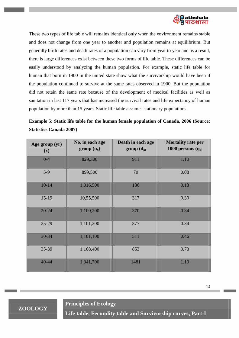
Example 5: Static life table for the human female population of Canada, 2006 (Source:

Statistics Canada 2007)

Age group (yr)

(x)

No. in each age

group (nx)

Death in each age

group (dx)

Mortality rate per

1000 persons (qx)

0-4 829,300 911 1.10

5-9 899,500 70 0.08

10-14 1,016,500 136 0.13

15-19 10,55,500 317 0.30

20-24 1,100,200 370 0.34

25-29 1,101,200 377 0.34

30-34 1,101,100 511 0.46

35-39 1,168,400 853 0.73

40-44 1,341,700 1481 1.10



15

45-49 1,336,900 2364 1.77

50-54 1,193,800 3338 2.80

55-59 1,054,000 4775 4.53

60-64 805,500 5729 7.11

65-69 636,800 7253 11.39

70-74 554,300 10,210 18.42

75-79 490,800 15,221 31.01

80-84 389,200 21,236 54.66

85-89 227,900 22,256 97.66

90 and more 125,300 38,742 309.19

Static life table (time specific, stationary or vertical) is constructed on the basis of cross

section of population at a given specific time. The above static life table is calculated on the

basis of census data and mortality data of Canada female population in 2006. This data can be

used to calculate the mortality rate and other life table components by assuming that the

population is stationary.

9. Application of life table

Life tables can be used to understand the patterns and causes of mortality of the individuals in

a population. It can also be used to predict the growth or decline of future populations and

also help in protecting the populations of endangered species.

Another very important application of life table is the prediction of growth and decline of

human populations. The growth or declining of the population of a country or given region



16

depends upon the number of children each person has and the age at which the individuals

die. Moreover, it is also important to note that the growth or decline of a population also

depends upon the age of the individuals at which they produce their offsprings. It is helpful in

providing the effects of changing patterns of survival as well as reproductive events on the

population dynamics.

Life tables can also be used in the field of species conservation efforts. For instance, in the

case of the loggerhead sea turtle of the southeastern United States. The population of

loggerhead sea turtle is declining and mortality of their eggs and hatchlings is very high.

These important information about sea turtle led conservation biologists to emphasize the

protection of their nesting beaches. When these measures were not proved very effective in

protecting the decline of sea turtle population, compiling and analyzing of their life table

indicated the reducing mortality of older turtles could provide a greater probability of

reversing the declining of these sea turtle population. Therefore, management efforts to

protect these turtle shifted to convincing the fishermen to install the device of turtle exclusion

on their nets to prevent the older sea turtles from drowning.

Life tables can be used to calculate the average longevity of a population for determining the

age composition of a population. It can also be used to indicate critical stages in the life cycle

of a species at which mortality rate is very high to make the differences between species, for

explaining success of same species in varied biotopes, for providing information of value in

fish exploitation (yield) as well as controlling of various agricultural and other pests.

6. Summary

A population can be defined as a group of individuals belonging to the same species.

Some population either have defined boundary while others do not have well

demarcated boundary.

Mortality is one of the important parameter which can explain the population change.

A life table can be expressed as summary of age specific mortality rates occurring in a

group of individuals of a given population.



17

Life table construction is a simple method to follow births rate, deaths rate and

reproduction in the given population.

Life tables are categorized into three types, cohort life table that observe the survival

of all individuals in a population from the time of birth to death, static life table

analyze the number of total number of individuals living at each age group in a

population and Dynamic composite life table is a composite of a number of animals

that are marked for a period of years instead at the time of birth only.

The first column (x) in a life table denotes age class and second column (nx) specify

the total number of individuals surviving at the starting of each age.

These two columns of the life table can be further used to find out several other life

history parameters, such as the proportion survival (lx), proportion of individuals in a

cohort dying at each age (dx) and age-specific mortality rate (qx) which is useful to

find the age at which mortality is maximum.

Static table makes assumptions that the population has a stable age structure and the

population size is stationary.

Study of life tables can be applied to understand the patterns of mortality, predicting

the growth or decline of future populations and also help in protecting the populations

of endangered species.

k Development Team - epgp.inflibnet.ac.in

Documents

Transcript of k Development Team - epgp.inflibnet.ac.in