(Just) first time lucky?The impact of single versus multiple bank lending relationships

on firms and banks’ behavior!.

Giorgia Barboni†and Tania Treibich‡

July 1, 2012

Abstract

The widespread evidence of multiple bank lending relationships in credit marketssuggests that firms are interested in setting up a diversity of banking links. How-ever, it is hard to know from the empirical data whether a firm splits the financingof one investment project across lenders or not, and whether such multiple lendingis symptomatic of financial constraints or rather a well-designed strategy. By set-ting up a controlled laboratory experiment we are able to uncover the conditionsfavoring multiple versus single lending strategies of borrowers, as well as improvingthe probability to get funding from lenders.Our results can be summarized as follows: first, we do find that, keeping everythingelse equal, risky and untrustworthy borrowers are more likely to choose multiple vis-a-vis single bank lending relationships. Second, the choice of multiple bank lendingrelationships is identified by lenders as a signal of ”bad quality” and borrowers whodecide to spread their funding request among several lenders su!er higher creditrationing. Third, we do observe, from the lenders’ side, that being chosen as firstas well as the length of the relationship positively a!ect the probability to lend.Finally, when information upon borrowers’ behavior is made available, lenders aremore likely to punish free-riding behaviors than simple default due to project fail-ure. Our results thus show that the reason why borrowers default matters for thecontinuation of the relationship lending.

!Preliminary and Incomplete. Helpful comments from John D. Hey, Georg Kirchsteiger, Luigi Marengoand seminar participants at CRED, University of Namur and Tilburg University are gratefully acknowl-edged. We also want to thank Paolo Crosetto for his unvaluable help and support provided. Financialsupport was provided by the LEM laboratory of the Scuola Superiore Sant’Anna and SKEMA BusinessSchool

†LEM, Sant’Anna School of Advanced Studies and University of Namur‡OFCE-DRIC, GREDEG, Universite Nice-Sophia Antipolis, SKEMA Business School and LEM,

Sant’Anna School of Advanced Studies

1

Keywords: Repeated Games, Information Asymmetries, Multiple Lending, Relationship

lending.

JEL codes: C72 C73 C92 G21.

1 Introduction

Early theoretical contributions on financial intermediation suggest that borrowing from

one bank is optimal as it reduces monitoring costs (Diamond, 1984) and the use of collat-

eral (Boot and Thakor, 1994). Consolidated evidence on multiple bank lending relation-

ships appears then to be at odds with these models: multiple bank lending relationships

have been extensively documented in credit markets, among firms of all size and ages. In

the US, for instance, 50% of firms borrow from more than one bank (Petersen and Rajan,

1994), while this share reaches 80% for Italian firms (Detragiache et al., 2000). As most of

the interactions between firms and banks are repeated through time, it may be optimal,

both for firms and banks, to establish more than one link. Indeed, it has been shown

that multiple bank lending relationships represent a mean to restore competition among

lenders and to limit ex post rent extraction (von Thadden, 1995), to mitigate ex-post

moral hazard behaviors (Bolton and Scharfstein, 1996) and to reduce the probability of

an early liquidation of the project (Diamond, 1991; Detragiache et al., 2000).

On the empirical ground, several works have tried to uncover the determinants of mul-

tiple bank links: higher frequency of multiple bank lending relationships is associated to

countries with ine!cient judicial systems and poor enforcement of creditor rights (Ongena

and Smith, 2000), to firms with a poor credit or performance record (Farinha and Santos,

2002) and to more opaque firms (Guiso and Minetti, 2010). In analyzing the determinants

of multiple bank lending relationships, these works encounter several endogeneity issues

which are only partly solved by appropriate econometric instruments. From one end of

the spectrum, firms’ quality is strictly correlated to their access to funds, and this in turn

a"ects their decision upon single versus multiple bank lending relationships. We refer to

this point as the ”credit rationing story”: as the borrower’s quality deteriorates, her access

to credit becomes more di!cult, and she might split her loan requests and ask smaller

amounts to a higher number of lenders. Such poor quality firm would therefore maintain

several credit links. It might also be the case that a firm chooses multiple lending as a ”di-

versification” strategy: maintaining diverse sources of funds helps to limit hold-up costs

associated with relationship lending. Moreover, playing the competition between banks

might further improve the firm’s contract conditions. On the other end of the spectrum,

firm’s creditworthiness is inherently related to relationship lending. With respect to this,

Petersen and Rajan (1994) and Berger and Udell (1995) have shown that when a borrower

builds a long-term relationship with the same lender, she can benefit from better credit

2

terms as well as access to further funds. The ”relationship lending story” thus a!rms

that the firm’s quality, by favoring long term relationships, is positively correlated with

borrowing concentration.

Both stories are plausible, and have been verified both theoretically and empirically. From

lenders’ perspective, benefits of relationship lending are due to a reduction of information

asymmetries from repeated interactions, and increased incentives for the firm to behave

in a good manner. However, observational data do not allow to identify which channel

develops more frequently and under which conditions. Therefore, a controlled labora-

tory experiment seems the most appropriate setting to answer to the following research

questions: is multiple lending explained by di!culties to build a stable relationship or

rather a strategy in order to diversify the sources of credit? To our knowledge, this is the

first experimental credit market to study the determinants of single versus multiple bank

lending relationships.

We build a laboratory experiment in which, in a similar spirit as Carletti et al. (2007),

lenders have limited diversification opportunities and are subject to ex-post moral hazard

problems. We then allow borrowers’ quality to vary exogenously and test how this a"ects

lenders’ funding decisions as well as borrowers’ choice between single and multiple bank

lending relationships. We first design a market in which there is no opportunity to create

long term relationships between borrowers and lenders. We then modify it by allowing

relations to be established through time. By comparing funding decisions and repayment

behavior, keeping riskiness constant, we are able to detect the impact of relationship lend-

ing as well as credit rationing on firms’ borrowing strategies. Finally, we further modify

the relationship lending setting by making the source of moral hazard (if any) public.

Our experimental design also allows to test for the emergence of social preferences in

addition to self-interested actions. In particular, by implementing a treatment in which

borrowers have the possibility to choose to which lender they want to address their fund-

ing request first, we are able to study lenders’ decision along two dimensions: from one

side, by comparing randomness with intentionality, we can study whether in a relationship

lending setting borrowers and lenders engage in a committed relationship, and reach the

cooperation equilibrium. From the other side, we can also test for the impact of ”not

being chosen” on the lender’s decision. In other words, we can analyze whether lenders

change their behavior depending on their rank in the borrowers’ lending requests. Besides,

we can also condition lenders’ decisions to single versus multiple bank lending strategies,

and see whether, ceteris paribus, lenders do behave di"erently. Laboratory experiments

are not new in the credit market literature: using an experimental credit market, Brown

and Zehnder (2007) show that information sharing between lenders works as an incentive

for borrowers to repay, when repayment is not third-party enforceable, as they anticipate

that a good credit history eases access to credit. This incentive becomes negligible when

interactions between lenders and borrowers are repeated, as banking relationships can

3

discipline borrowers. Similarly, Brown and Zehnder (2010) find that asymmetric informa-

tion in the credit market has a positive impact on the frequency of information sharing

between lenders, whereas competition between them may have a negative, though smaller,

e"ect on information sharing.

Closer to our paper are the laboratory experiments conducted by Fehr and Zehnder (2009)

and Brown and Serra-Garcia (2011): both papers analyze how borrowers’ discipline is af-

fected by debt enforcement and find that (strong) debt enforcement has a positive impact

on borrowers’ discipline. However, when debt enforcement is weak, Brown and Serra-

Garcia (2011) show that bank-firm relationships are characterized by a lower credit vol-

ume.

We contribute to the empirical literature on multiple bank lending relationships along

three directions: first, we show that firms tend to use multiple bank lending relation-

ship in an opportunistic way, as more dishonest firms tend to have multiple bank lending

relationships, irrespectively of their riskiness. Second, contrary to our expectations, re-

lationship lending does not seem to have an impact on the choice between single and

multiple bank lending relationships. Finally, we show that firms are less credit rationed

when they concentrate their credit. This result is in line with the recent work on the

financial crisis: De Mitri et al., 2010, for example, have shown that firms with higher

borrowing concentration have been less hit by the credit tightening.

The rest of the paper is organized as follows. Section 2 describes the experimental design,

outlining predictions. Results are reported in Section 3. Section 4 concludes.

2 The Model

Our lending game builds on the investment game introduced by Berg et al. (1995), where

the lending as well as repayment decisions relate to the economic characteristics of the

borrower and the screening and enforcement capacities of the lender. In order to study

borrowers’ funding strategies as well as lenders’ decisions, we introduce several novelties.

Lending contracts and relationships are endogenously formed, as is reputation. However,

interest rates and project types are exogenously given, while project returns are stochas-

tic, as in Fehr and Zehnder (2009). The enforcement of debt repayment is incomplete as

we allow for strategic default from the borrower. Information about the borrower’s risk

level as well as her trustworthiness is incomplete, but we allow for information sharing

among lenders: they observe default events in a Credit Register. Again, similar to Fehr

and Zehnder (2009), borrowers don’t have any initial endowment and cannot use excess

returns in the future rounds of the game. However, contrary to their design, we assume

that, if the borrower is not able to conclude the credit contract, she has no access to any

alternative project. Similarly, lenders cannot invest in a safe project and therefore they

compete against each other in order to enter the game: the value of both the borrower’s

4

and the lenders’ outside option is normalized to zero.

Throughout the game, we observe players’ decisions keeping constant price (interest rates),

risk (the project’s fixed success probability) and information (using a Credit Register, as

in Brown and Zehnder (2007)). Our experimental credit market involves three subjects,

one borrower and two lenders. Each participant is randomly assigned to her role at the

beginning of a session. The roles remain the same throughout the session, which lasted

T periods. The number of periods was not disclosed to the subjects in order to prevent

any backward induction strategies, and was randomly drawn for each session.

2.1 Basic Setup

We start with an ex-post moral hazard model with an infinite number of identical games.

For each game !i, a borrower i needs to finance an investment project which requires

D units of capital to become profitable. We assume that the borrower has not enough

wealth to implement her project by herself. Therefore, she has to turn to the credit mar-

ket, which consists of k identical lenders where k = {1, 2}, who can lend up to D units

of capital. The borrower pays s every time she faces a lender. By s, we identify the

“administrative costs” faced by the borrower at each bank, that is, all costs the borrower

has to sustain in order to go to a bank and ask for a loan (mainly administrative and

bureaucratic costs)1. We assume that the borrower has enough collateral to advance her

funding request to both lenders (c = 2s, where c < D).

The borrower moves first and chooses whether she wants to borrow D from only one

lender (Full decision), or, rather, to borrow D2 from each lender (Partial decision). This

is how we design single versus multiple bank lending relationships. In the basic setup,

Nature then determines who between l1 or l2 enters the game first, with equal probability.

After receiving the application fee s, the chosen lender is asked to take the second move

which is to accept or deny the loan request. Lenders can only accept or reject the loan

request they have received (e.g. they cannot lend D2 if they have been requested D). We

assume that each lender will lend with probability "k, where k = {1, 2}2.

Neither the borrower nor the lenders know who has been chosen to enter the game first.

The lenders only know whether in the round they have been requested to enter the game

or not, and the size of loan requested by the borrower.

After the first lender has made his decision, the second lender might be asked to enter the

game if the borrower has obtained less than D (this is the case in the Partial subgame

and in the Full subgame conditional on the first lender having denied credit). In that

1In other words, s represents the fee the borrower has to pay in order to open the account, or thetransaction fee, and it enters the bank’s turnover. The lender will receive s irrespectively of whether theloan is issued or not.

2For ease of notation, we call !1 (!2) the probability that the lender (randomly) chosen to play first(the lender chosen to play second) gives the loan.

5

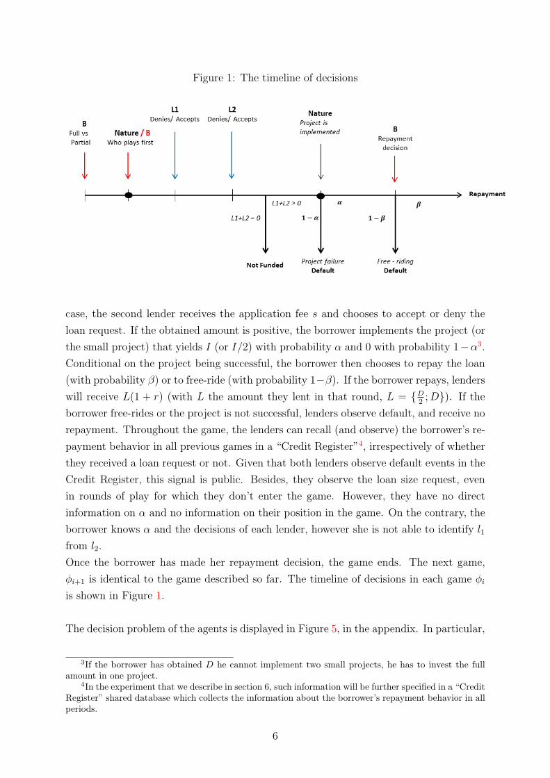
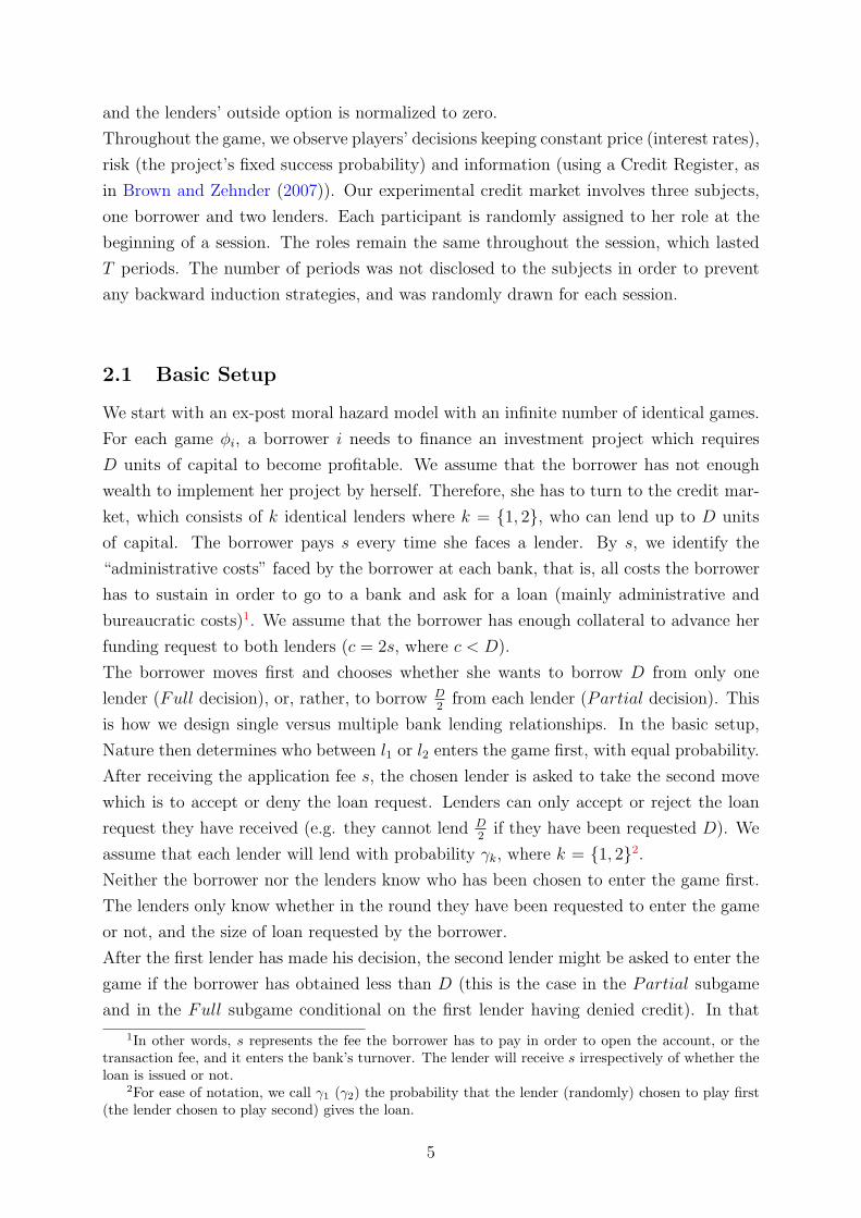
Figure 1: The timeline of decisions

case, the second lender receives the application fee s and chooses to accept or deny the

loan request. If the obtained amount is positive, the borrower implements the project (or

the small project) that yields I (or I/2) with probability # and 0 with probability 1"#3.

Conditional on the project being successful, the borrower then chooses to repay the loan

(with probability $) or to free-ride (with probability 1"$). If the borrower repays, lenders

will receive L(1 + r) (with L the amount they lent in that round, L = {D2 ; D}). If the

borrower free-rides or the project is not successful, lenders observe default, and receive no

repayment. Throughout the game, the lenders can recall (and observe) the borrower’s re-

payment behavior in all previous games in a “Credit Register”4, irrespectively of whether

they received a loan request or not. Given that both lenders observe default events in the

Credit Register, this signal is public. Besides, they observe the loan size request, even

in rounds of play for which they don’t enter the game. However, they have no direct

information on # and no information on their position in the game. On the contrary, the

borrower knows # and the decisions of each lender, however she is not able to identify l1

from l2.

Once the borrower has made her repayment decision, the game ends. The next game,

!i+1 is identical to the game described so far. The timeline of decisions in each game !i

is shown in Figure 1.

The decision problem of the agents is displayed in Figure 5, in the appendix. In particular,

3If the borrower has obtained D he cannot implement two small projects, he has to invest the fullamount in one project.

4In the experiment that we describe in section 6, such information will be further specified in a “CreditRegister” shared database which collects the information about the borrower’s repayment behavior in allperiods.

6

the borrower’s profit will be:

#B =

!"""""""""""""""""""""#

"""""""""""""""""""""$

"2s if no loan ("1 = "2 = 0)

#[I "D(1 + r)]" s if loan is repaid, Full strategy ("1 = 1; $ = 1)

#[I "D(1 + r)]" 2s if loan is repaid, Full strategy ("1 = 0; "2 = 1; $ = 1)

or Partial strategy ("1 = 1; "2 = 1; $ = 1)

#[ I2 "

D2 (1 + r)]" 2s if loan is repaid, Partial strategy (("1 = 0; "2 = 1) # ("1 = 1; "2 = 0); $ = 1)

#I " s if strategic default, Full strategy ("1 = 1; $ = 0)

#I " 2s if strategic default, Full strategy ("1 = 0; "2 = 1; $ = 0)

or strategic default, Partial strategy ("1 = 1; "2 = 1; $ = 0)

# I2 " 2s if strategic default, Partial strategy (("1 = 0; "2 = 1) # ("1 = 1; "2 = 0); $ = 0)

On the contrary, the first and second lender’s profit will be respectively:

#L,1 =

!"""""""""#

"""""""""$

s if no loan ("1 = 0)

#Dr + s if loan is repaid, Full strategy ("1 = 1; $ = 1)

#D2 r + s if loan is repaid, Partial strategy ("1 = 1; $ = 1)

"D + s if strategic default, Full strategy ("1 = 1; $ = 0)

"D2 + s if strategic default, Partial strategy ("1 = 1; $ = 0)

and

#L,2 =

!""""""""""""#

""""""""""""$

0 if Full strategy ("1 = 1)

s if no loan ($"1; "2 = 0)

#Dr + s if loan is repaid, Full strategy ("1 = 0; "2 = 1; $ = 1)

#D2 r + s if loan is repaid, Partial strategy ($"1; "2 = 1; $ = 1)

"D + s if strategic default, Full strategy ("1 = 0; "2 = 1; $ = 0)

"D2 + s if strategic default, Partial strategy ($"1; "2 = 1; $ = 0)

2.2 Case with complete information

In a first step we present the equilibrium in the setting with complete information, then

we will relieve this assumption and do not let the lenders know the risk level of the project,

#, nor the borrower’s discount factor, %. All players observe the outcome of all previous

stages before the current stage begins.

2.2.1 The finite-horizon game

In a game with finite horizon, lenders’ problem is to decide whether to accept or deny the

borrower’s request for funding (with probability "k) subject to the borrower’s incentive

7

compatibility constraint. As all players know when the game will come to end, they can

use backward induction strategies.

In particular, once the project has succeeded, the borrower (player i) will choose to repay

or not by comparing her profit in both cases. She will prefer to repay her debt rather

than free-ride if and only if the following constraint is satisfied:

#B,repay % #B,default (1)

If the borrower chooses to request the entire amount to one lender at the time (playing

Full), condition 1 is only satisfied for D(1 + r) & 0. It is straightforward to see that this

condition implies that the borrower will always default in this type of game, by choosing

to free-ride on the loan (therefore the amount repaid D(1 + r) is equal to zero).

When asked to enter the game, the lender’s maximization problem is to choose a value

of "k (k = {1, 2}), his probability to give the loan to the borrower, which maximizes his

profit.

We proceed by backward induction and compute the lender’s profit as follows:

max!

#L,k = "k(s"D) + (1" "k)s (2)

where "!k = 0 is the decision which maximizes the lender’s profit. Therefore, the lender’s

optimal strategy in the finite-horizon game is not to lend, knowing that the borrower

would never repay. It is important to notice in this case that, as the probabilities that the

two lenders are chosen to play first are i.i.d., the solution of the game as presented in 2 is

identical for both lenders. Besides, as the probability that the second lender will enter the

game depends upon the decision of lending of the first lender, by backward induction we

get that, given that "!1 = 0 for the first lender, the second lender will automatically enter

the game but will face the same maximization problem as the first lender, thus finding his

optimal solution in not-lending, himself ("!2 = 0). In the equilibrium of the single lending

case, players thus reach the end node number 3.

If the borrower instead opts for multiple bank lending relationships (playing Partial), her

decision conditional on receiving funding will be exactly the same as in 1 only that S is

always equal to 2s. At end nodes 5 and 6, the amount obtained is L = D/2 while at end

node 4 it is L = D. In all cases, condition 1 requires D(1+ r) & 0 and the borrower never

repays.

Lenders’ profit in the multiple lending setting is now #L,k = "k(s " D/2) + (1 " "k)s.

Again, the solution of the maximization problem for lenders is to refuse lending. In the

equilibrium of the multiple lending case, players thus reach the end node number 7.

Given the equilibria obtained above, the final payo" of the borrower is always #B = "2s.

Thus the borrower is indi"erent between choosing the single lending or the multiple lending

strategy.

8

2.2.2 The infinite-horizon game

The game !i is repeated an infinite number of times.

In the first period of this model, when the borrower takes the decision of repaying the

loan or not, she compares the present value from cooperating, Vc to the present value

from defecting Vd. We solve the model in the case of a “trigger” strategy: there is no

cooperation after the first defection. Thus repaying today allows for cooperation in the

future while defecting prevents it.

If the borrower chooses to play Full, she asks the entire amount to one lender at the time,

the incentive compatibility constraint of the borrower now becomes:

Vc,B > Vd,B (3)

where

Vc,B ="%

t=1

%t#1 [#[I "D(1 + r)]" s]

and % ' [0;1] is the subject’s time discount rate.

Defecting in each period means to receive #I " s in the first period and paying the fee s

to both lenders in all subsequent periods without receiving any loan 5:

Vd = #I " s +"%

t=2

%t#1("2s)

the borrower thus cooperates if the following condition is satisfied:

# >"%s

%I "D(1 + r)(4)

We call #! the threshold value at which the borrower changes her decision, with

#! = #"s"I#D(1+r)

6. Thus we get the following decisions of the borrower in the single lending

case:

$ =

!#

$0 if # < #!

1 if # % #!

In the Partial case, she asks half of the amount to each lender, and pays the fee S = 2s

for sure. As a consequence, the borrower cooperates if #[%I " D(1 + r)] > 0, that is,

5Indeed, both lenders observe free-riding in the first period before taking their decision in the subse-quent periods

6Given our parametrization, we can expect a threshold value "! = 0, 6 for a value of the discountfactor # = 0, 45. Notice that the expression on the right is negative for # > D(1+r)

I = #!, thereforecooperation is always satisfied for # ']#!; 1]. If # ' [0; #!] the equilibrium depends on the value of ".Moreover, if # = 0 and " > 0 then the condition is never satisfied : an extremely impatient individualbehaves as if it were a one-shot game.

9

% > D(1+r)I . Setting %! = D(1+r)

I , we get the following decisions of the borrower in the

multiple lending case:

$ =

!#

$0 if % < %! $#

1 if % % %! $#

In order to make his decision, the lender compares his expected value from cooperating

or not. The lender accepts to give the loan if :

Vc,L > Vd,L (5)

with

Vc,L ="%

t=1

%t#1 [$#L(1 + r)" L + s]

and

Vd,L ="%

t=1

%t#1s

Expression 5 is true if $# > 11+r

7. Both the project’s risk level and the borrower’s

trustworthiness matter in lenders’ decision. The size of the loan (L = D in the Full

branch and L = D/2 in the Partial branch) does not a"ect the threshold of making

lending profitable, however the borrower’s trustworthiness is defined di"erently in the

case of single or multiple lending (see above). Thus lenders’ decision, for k = 1, 2 follow

the condition :

"k =

!#

$0 if # < 1

1+r $$

1 if # % 11+r and $ = 1

If the project is too risky, the lender has no incentive to accept the borrower’s request,

whatever her behavior. However, if the project is safe enough, it is the borrower’s behav-

ior (defined by her discount factor %) that conditions lending.

We now turn to the analysis of borrower’s choice between single and multiple bank lending

relationship. According to the analysis we have conducted so far, the borrower will prefer

single bank lending relationships as long as the following inequality is satisfied:

Vsingle,B > Vmultiple,B (6)

7Notice that for " high enough (" > "! and " > 11+r ), the lenders’ and the borrowers’ incentives

align. Moreover, for 11+r > "!, the lender’s threshold is binding. Figure 4 however shows that which

threshold between the lenders’ (with "!! = 11+r ) and the borrower’s is binding depends on the borrower’s

patience.

10

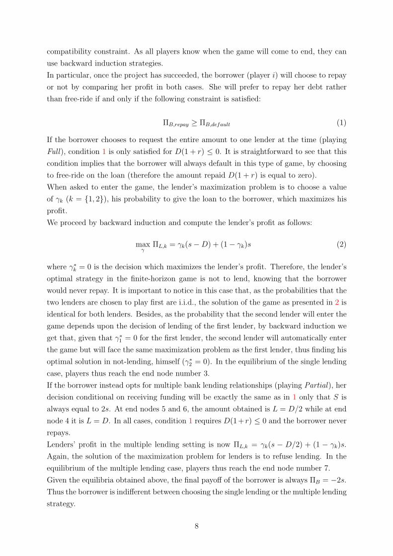
with

Vsingle,B = $

& "%

t=1

%t#1[#[I "D(1 + r)]" s]

'+ (1" $)

&#I " 2s +

"%

t=2

%t#1("2s)

'

and

Vmultiple,B = $

& "%

t=1

%t#1[#[I "D(1 + r)]" 2s]

'+ (1" $)

&#I " 2s +

"%

t=2

%t#1("2s)

'

Figure 2: Single vs Multiple lending choice, $ = 1

Figure 3: Single vs Multiple lending choice, $ = 0

With few algebraic passages it is easy to see that the borrower should always prefer

single to multiple bank lending relationships if she believes that "1 = 1, that is she will

receive credit in the first period. What may further a"ect such decision is the possibil-

ity that the probability to receive credit in the first period depends on the size of the

loan request. However, we have seen above that loan size does not a"ect lending, if the

11

Figure 4: #! and #!! as function of %, single lending

Note: both thresholds are equal at #!! = D(1+r)I+s(1+r) .

Moreover, there is no value of "! for # = #!.

borrower repays. Figures 2 and 3 show that keeping the borrower’s repayment strat-

egy riskiness level fixed, the di"erence in her payo"s when choosing a single or multiple

lending strategy is marginal whatever the value of %. However, when considering such

di"erence across riskiness levels, keeping the borrower’s discount factor fixed (figures on

the left), the single lending bonus is increasing in the value of # when the borrower is

trustworthy. Therefore the safer the borrower’s profile, the higher the incentive to choose

single lending. Untrustworthy borrowers in turn benefit from a fixed bonus when choosing

single lending. Indeed, single lending reduces the cost associated to the loan request as

long as the first lender accepts to give funding, which is the case only in the first period

when the borrower is untrustworthy. We can therefore introduce the following hypotheses:

Hypothesis 1: The single lending strategy strictly dominates the multiple lending one.

The repeated game with complete information predicts that no contract will be formed

in the case of risky or untrustworthy borrowers. On the contrary, repeated contracts will

be formed between the borrower and the first lender to be chosen if the project is safe and

the borrower has incentives to be trustworthy. Thus both riskiness and trustworthiness

have to be combined to allow for cooperation to emerge.

2.3 Solving the game with incomplete information

We now relieve the assumptions that lenders know the riskiness of the project and the

borrower’s discount factor. Therefore, a lender has to form beliefs on the probability to be

repaid in order to make his lending decision. In the finite horizon game, lenders’ decisions

12

do not depend on their knowledge of those parameter values, thus the equilibrium will

also be, by backward induction, not to lend, knowing the borrower would free-ride. In the

infinite horizon game instead, both the riskiness of the project and the trustworthiness of

the borrower matter. In the case with complete information, the probability to be repaid

is defined by pR = $#. Lenders accepts to lend if the probability to be repaid is high

enough: pR > 11+r . However, with no information on $ and #, lenders need to compute

a proxy pRt which is reevaluated in each period. In the first period of the game, lenders

have no information about the riskiness of the project, thus they use their prior pR0 on

the value of the probability to be repaid in order to decide whether to lend or not in the

first period. If the prior is above 11+r a lender would accept, and refuse in the alternative.

In this latter case, the player will refuse to lend in all subsequent periods if he has no new

information. However, if contracts are formed by him or the other lender, the player will

use observed default events in order to compute his belief over pR in each period. The

frequency of defaults is the proxy used by lenders:

pRt =

Defaulttt

(7)

Lenders can both recover the number Defaultt in each period using the Credit Register,

which is public information8. Starting from a high prior (pR0 > r

1+r ), a player can stop

lending if observed defaults are too frequent. On the contrary, starting from a low prior

(pR0 & r

1+r ), and if some contracts are actually formed by the other two players, a lender

can start giving funds after observing enough repayments. However, if both lenders start

with low priors, no contracts will be formed in all subsequent periods.

Introducing asymmetry of information about the project riskiness and borrower’s patience

constrains lenders to reevaluate the borrower’s probability to repay in each period, based

on the available information. We can therefore introduce the following hypothesis:

Hypothesis 2: There is a negative relation between observed defaults and the probability

to get funds.

3 Treatments

The experiment was implemented at the EXEC, University of York in October 2011.

All subjects were volunteers, and each subject could only take part in one session. All

8There is one way however that lenders can disentangle the borrowers’ repayment behavior from theriskiness of the project. Indeed, her decision on repaying or not ($) is defined by the following rule: $ = 1if " > "! and $ = 0 if " & "!. Therefore we get the following probabilities to repay: pR = " if " > "!

and pR = 0 if " & "!. Thus any repayment event observed by the lender is enough to signal that theborrower will always repay if she can ($ = 1). Still, we have seen that the order of the thresholds "! and"!! depends on the borrowers’ patience #. The repayment event therefore contains information about "but it is ambiguous due to the uncertainty about the borrower’s patience.

13

participants were undergraduate students of the University of York. We conducted six

experimental sessions, for a total of 129 subjects. To ensure that the subjects understood

the game, the experimenters read the instructions aloud and explained final payo"s with

the help of tables provided in the instructions9. Before the game started, the subjects

practiced three directed test runs. In each session, groups of three subjects were formed:

one borrower (Player A) and two lenders (Players B and C). All subjects received a show-

up fee of 5 pounds to which their payo" in the game was added in order to compute their

final payo". The players earned an average of 13 pounds from participating in the game.

At the end of the game, the subjects randomly selected one of the periods of play to be

the one that was actually paid. If the payo" achieved in this period were to be negative,

subjects lost part of the show-up fee. Each session lasted approximately one hour an a

half.

We implement three treatments in order to detect the e"ect of borrowers’ riskiness, the

identification of lenders and information disclosure on subjects’ decisions. In each treat-

ment, we identify the borrower as player A, while the two lenders as player B and player

C. Treatments were constructed as follows. In the Random treatment (hereafter “RA”,

the baseline treatment), who plays first between player B and player C is randomly set10.

In the Relationship lending treatment (hereafter, “RL”), at the beginning of each round,

player A is asked to choose to play first with player B or player C. In the Relationship

lending treatment (hereafter, “RL”), at the beginning of each round, player A is asked

to choose to play first with player B or player C. The Information Disclosure treatment

(hereafter “ID”) is identical to the RL treatment with the only exception that it allows

player B and player C to know whether player A’s default has to be accounted for in-

vestment failure or free-riding. This information is only accessible to the player(s) who

entered this particular round of play.

For each treatment, we ran two separate sessions11, a safe project session (#low) and a

risky project one (#high)12. Therefore, we ran a total of six sessions (see Table 1 below).

3.1 Safe vs Risky treatments

If lenders had perfect information on the borrower’s riskiness, we might have expected a

higher share of successful contracts in the case of the safe treatments (# = #high) from the

beginning. In a setting with asymmetric information about #, through repeated interac-

tion, players should adapt their beliefs over the borrowers’ overall quality (combination

9See the instructions in the Appendix. We only provide here the instructions for the ”Random”treatment. Instructions for the ”Relationship Lending” and the ”Information Disclosure” treatments arealso available upon request.

10with equal probability that either player B or player C is selected as the first lender. In the experi-ment, the choice of Nature was generated by computer.

11Each participant played in only one session12where I"low < I"high.

14

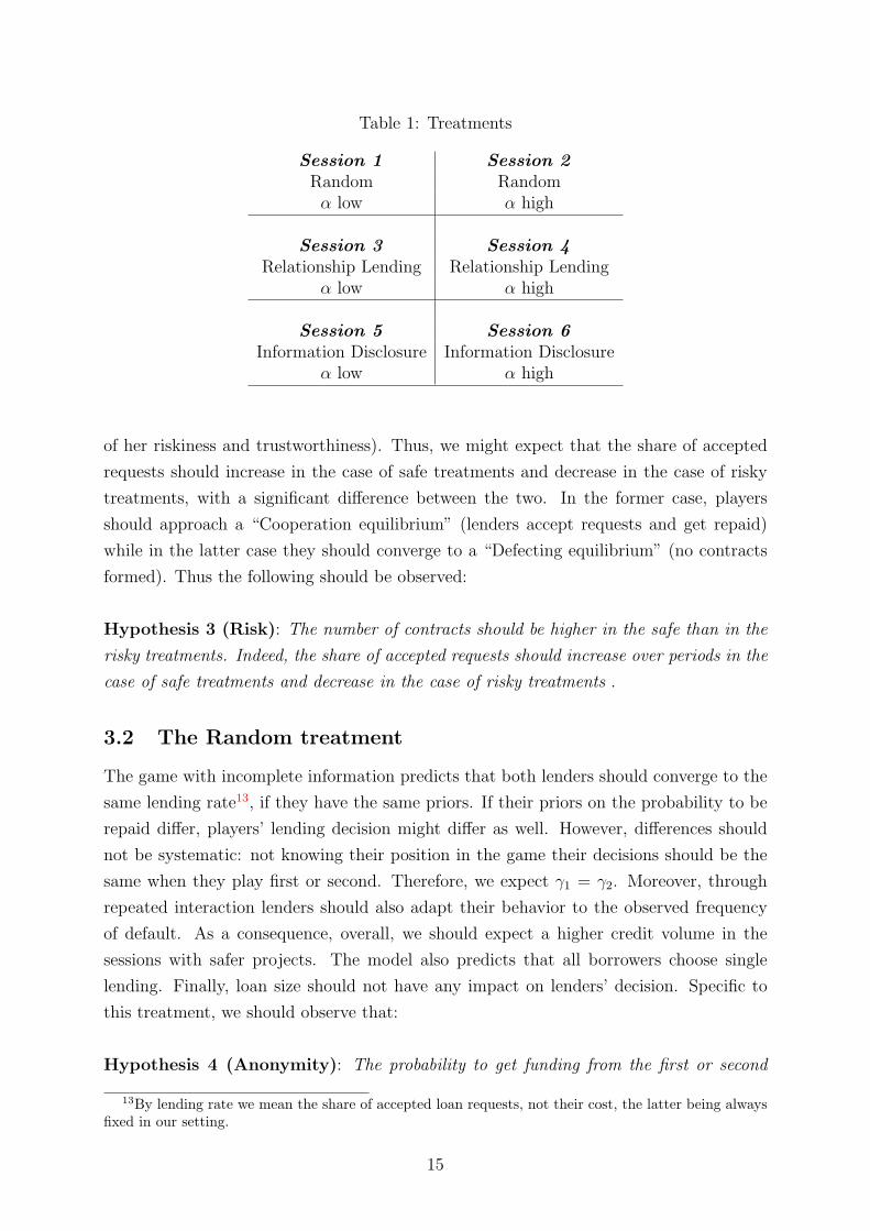
Table 1: Treatments

Session 1 Session 2Random Random# low # high

Session 3 Session 4Relationship Lending Relationship Lending

# low # high

Session 5 Session 6Information Disclosure Information Disclosure

# low # high

of her riskiness and trustworthiness). Thus, we might expect that the share of accepted

requests should increase in the case of safe treatments and decrease in the case of risky

treatments, with a significant di"erence between the two. In the former case, players

should approach a “Cooperation equilibrium” (lenders accept requests and get repaid)

while in the latter case they should converge to a “Defecting equilibrium” (no contracts

formed). Thus the following should be observed:

Hypothesis 3 (Risk): The number of contracts should be higher in the safe than in the

risky treatments. Indeed, the share of accepted requests should increase over periods in the

case of safe treatments and decrease in the case of risky treatments .

3.2 The Random treatment

The game with incomplete information predicts that both lenders should converge to the

same lending rate13, if they have the same priors. If their priors on the probability to be

repaid di"er, players’ lending decision might di"er as well. However, di"erences should

not be systematic: not knowing their position in the game their decisions should be the

same when they play first or second. Therefore, we expect "1 = "2. Moreover, through

repeated interaction lenders should also adapt their behavior to the observed frequency

of default. As a consequence, overall, we should expect a higher credit volume in the

sessions with safer projects. The model also predicts that all borrowers choose single

lending. Finally, loan size should not have any impact on lenders’ decision. Specific to

this treatment, we should observe that:

Hypothesis 4 (Anonymity): The probability to get funding from the first or second

13By lending rate we mean the share of accepted loan requests, not their cost, the latter being alwaysfixed in our setting.

15

lender should be equal.

3.3 The Relationship Lending treatment

We modify the above described game (defined as the Random treatment), by allowing

the borrower to choose l1 or l2 to enter the game first, at the beginning of each round

of play, instead of Nature. Furthermore, lenders are informed of their position in the

game. We define as pchosen1 the probability that player l1 is chosen as first (such that

pchosen2 = 1 " pchosen1), with pchosen1 being endogenously determined by the borrower’s

choice in each period. The game then proceeds exactly as in the Random Game. However,

this time, when one lender receives a loan request from the borrower, his decision about

lending not only will depend upon the borrower’s past repayment behavior (that is, by

his beliefs over # and $), but also upon the fact that the borrower has voluntarily chosen

him instead of the other lender.

Assuming complete information, in the finite-horizon game, the borrower’s incentive-

compatibility constraint will be exactly as in equation 1: therefore, her optimal decision

will be to default. Besides, she will also be at most indi"erent between choosing one

lender instead of the other. Therefore, lenders’ optimal strategy under the finite-horizon

game is to deny credit, knowing that the borrower would never repay.

However, with the repetition of the game, the issue for lenders becomes to know whether

they gain from being chosen to play first or not. As before, if the project is too risky or

the borrower untrustworthy ($# < 11+r ), their decision will be to deny funding, whatever

their position in the game. However, if the project is safe enough, and the borrower

chooses the single lending strategy, she will form a contract with the first lender to play,

and the second lender will not enter the game. In that case, the first lender makes a

positive profit and the second lender no profit at all. Therefore, both lenders compete in

order to play first, that is increase their probability to be chosen pchosen,k, for k = a, b.

However, because lenders are only incentivized to increase pchosen,k in the profitable range

of #, where they both would accept to give the loan anyway, there is no way they can

di"erentiate one from the other. Therefore the predictions of the relationship lending

game are exactly the same as the random one.

Interesting e"ects can however emerge when we consider the game with imperfect infor-

mation, as implemented in the experiment. Indeed, when lenders are uncertain about the

default probability, they might interpret repeated matching as a signal of trustworthiness,

and increase their expected repayment probability as a consequence. This can be tested

by measuring the probability to give funds conditional on the length of relationship be-

tween the borrower and one of the lenders.

The possibility to identify the lender and choose which lender plays first (in the RL and

ID treatments) should increase lending and repayment behavior probability, as well as

16

relationship length: as trust is built up both players have higher incentives to cooper-

ate. Relationship lending could therefore mitigate risk: if the borrower’s fixed quality

element is poor (the project is risky), its endogenous element is improved (the borrower is

trustworthy). Thus a trade-o" between risk and trustworthiness could help improve risky

borrowers’ access to funding.

In the case that both lenders do not take their decisions simultaneously, but sequentially,

additional information can be inferred from the unfolding of the stage game. This is the

case in the “Full” branch, when l1 denies funding and the borrower goes to the second

lender. The second lender knows his position in the game and thus this is the only case

in which the action of l1 is disclosed to l2 (if l1 had accepted, l2 would not play). This

indirect information might also a"ect "2: the second lender can reevaluate the probability

to be repaid based on the decision of the first lender.

Hypothesis 5 (Lender order): The probability to get funding from the first or second

lender should be di!erent in the full branch only. However, being chosen should not a!ect

the probability to give funds.

3.4 The Information disclosure treatment

In this third treatment lenders participating in the round are told when default is caused

by the borrower’s voluntary free-ride. As commented above, after being given such infor-

mation, the lender should stop lending at all: whatever the value of #, the probability to

be repaid in all subsequent rounds is expected to be zero, if $ = 0. This e"ect should

act as an enforcement device and increase borrowers’ repayment probability, and, in turn,

credit volume conditional on no free-riding history should be relatively higher than in the

RL treatment. The possibility given to lenders to disentangle riskiness from trustworthi-

ness in the Information Disclosure treatment should therefore drastically limit free-riding

behaviors: borrowers could no longer use the benefit of the doubt to free-ride.

Hypothesis 6 (Free-riding disclosure): Free-riding behaviors should be lowest in the

ID treatment as compared to the RA and RL ones.

Corollary: The probability to give funds ("k) should be highest in the ID treatment as

compared to the RA and RL ones.

4 Results

In this section we report the results of the six experimental sessions. After presenting

descriptive statistics over the entire sample as well as by session, we investigate further

17

the determinants of players’ choices.

4.1 Descriptive Statistics

We start investigating our data with summary statistics in order to get a first intuition on

players’ behavior. Figure 6 in the Appendix shows borrower’s repayment behavior, while

figure 8 reports the lending decision by the first and the second lender. By comparing the

three figures, it is straightforward to see that lenders’ behavior displays a higher variability

than borrowers’. While the distribution of borrowers’ decisions is clearly unimodal, or, in

other words, we observe a very low degree of strategic default, the distribution of lenders’

decisions is, instead, bimodal. Indeed, although a significant share of lenders always

accept the borrowers’ request, most of them deny funding most of the time.

When it comes to multiple vs single lending strategies, Hypothesis 1 seems verified: the

full choice is observed most of the times (above 68% in all sessions), although not always

(see tables 4 to 6).

Next we test whether the size of the loan request a"ects lenders’ decision: when we

condition " on the choice of single versus multiple bank lending relationship, we see that

lending rates increase with loan size (figure 11, bottom).

We also perform a series of paired t-tests in order to compare di"erent values of " both

across lenders (by order) and treatments. When chosen as first, 48% of lenders accepted

the funding request , while only 28% gave credit when chosen as second. Such di"erence

is statistically significant. Results from the t-test don’t change when we restrict the

sample only to the Relationship Lending and Information Disclosure treatments, where

the borrower’s choice upon which lender she wants to address her funding request first

is made voluntary. Both t-tests thus run in favour of the argument that lenders tend to

positively respond to borrowers’ willingness to cooperate. At the same time, however,

they confute the predictions we made under Hypothesis 4: the order in which lenders

enter the game matters for the borrower’s probability to receive funding.

We then relate lenders’ order and their willingness to lend to the borrowers’ choice in

terms of single versus multiple bank lending relationships. Further, we find that the order

of requests matters only when the borrower has chosen the single-lending strategy (as

proxied by the Full choice), while we find no statistically significant di"erence between

the willingness to lend by the first and the second lender when the borrower has chosen

the multiple-lending strategy (as proxied by the Partial choice).

4.1.1 Safe vs risky treatments

We then compare players’ decisions across treatments. Although borrowers’ repayment

rate is always high (above 70% in all sessions), they repay more in safe treatments com-

pared to risky ones. The e"ect of riskiness on players’ decisions is therefore in accordance

18

with Hypothesis 3. This is further confirmed by figures 7 and 10 (top): lenders are able

to identify borrowers’ probability to repay given that they mostly refuse lending in the

risky treatments, while they accept significantly more14 in safe treatments. Moreover,

figure 9 compares the evolution of lenders’ decisions over time in the case of safe or risky

treatments. It is very clear that starting from a similar prior ("0 = 0, 6), lenders adapt

their beliefs over the probability to be repaid over time, following expectations from the

game with incomplete information. In the case of the safe treatments, with a low rate of

default, lending rates are very stable and comprised between 60 and 80%. In the case of

risky treatments on the contrary lending rates are strictly decreasing, reaching 20% at the

end of the game. Indeed, it takes time for lenders to learn the risk level of the borrower.

Table 4 presents summary statistics for our two corresponding sessions when the order of

the lenders in each period is randomly determined (Random Treatment-#low and Random

Treatment-#high15). As shown in columns (5) and (6), we test whether mean di"erences

across levels of riskiness are significant, for each decision variable. Not surprisingly, there

is more cooperation between players in the safe sessions, and the mean distribution of

all variables is significantly higher in the #high session than in the #low one. In the safer

session, borrowers are more willing to repay and lenders are more willing to lend. This is

further confirmed by the fact that in the safer session, even in the absence of relationship

lending, borrowers experience less credit rationing (the share of Rationed borrowers is

significantly lower)16.

Moreover, borrowers exogenously endowed with a risky project are more willing to opt for

multiple bank lending relationships than safe borrowers (the share of Full choice is lower).

However, the analysis here doesn’t allow us to understand whether this result is driven

by risk-diversification motives or, rather, by strategic behavior. We will specifically test

the determinants underlying borrowers’ choices in the following section.

Finally, when lenders don’t know their position in the game (RA sessions), the first and

second lender’s behavior should not di"er systematically (Hypothesis 4). If we find that

in the risky session there is no significant di"erence between the willingness to lend of the

first and the second borrower, this di"erence becomes significant in the safe one, against

theoretical expectations.

4.1.2 Random vs relationship lending treatments

Introducing relationship lending (RA vs. RL, figure 10, middle) also a"ects lenders’ will-

ingness to lend. As in Petersen and Rajan (1994), when relationship lending is possible,

we observe a stronger commitment from the parts. In particular, we find that the prob-

14Mean tests confirming the di!erences across treatments are shown in tables 4 to 6 and commentedbelow.

15Tables 5 and 6 show that similar results are found in the Relationship Lending and InformationDisclosure treatments.

16The construction of all variables is detailed in the Appendix.

19

ability to be given funds increases in RL treatments as compared with RA ones, and

repayment rates (figure 11) are higher when the lending relationship is stable.

The intuition behind these results is that, as theory predicts, in a stable relationship

lenders acquire more information on the borrowers’ riskiness and creditworthiness. More-

over, being chosen here plays a role, along two directions: from one side, being chosen

increases the lending rate; from the other, not being chosen seems to trigger a retaliation

behavior. Indeed, the lender who enters the game by default (because the first lender de-

nied funding) is less likely to give the loan as compared to when the decision is randomly

set. Results from table 5 also indicate that relationship lending doesn’t seem to mitigate

moral hazard behavior: repayment rates across risk levels are not statistically di"erent.

A possible explanation for this latter evidence is that the repayment rate is already very

high (greater or equal than 80%) in both sessions.

Furthermore, the share of single bank lending relationships in the risky session of the Re-

lationship Lending Treatment is significantly lower than the share of single bank lending

relationships in the risky session of the Random Treatment. A possible explanation is

that borrowers need to signal their creditworthiness to lenders in order to increase their

probability to receive funds. In the random treatment they only have one means to do

this and it is by choosing a single lending strategy. In the RL treatments however the

signaling process is more directly made by repeatedly choosing the same lender. In that

case, the choice of single vs multiple lending strategies loses its signaling importance. We

will further test this statement in the regression analysis.

4.1.3 Relationship lending vs Information Disclosure treatments

The Information Disclosure treatment only di"ers from the Relationship Lending Treat-

ment in the type of information lenders receive about the borrower’s behavior. Indeed,

while in the Relationship Lending treatment the source of default - whether it depends

upon project’s failure or borrower’s unwillingness to repay - was kept undisclosed, in the

ID sessions, instead, it is revealed to the lender su"ering losses.

Disclosing information (RL vs ID, figure 10, bottom) also a"ects lenders’ willingness to

lend, however, not exactly as predicted in Hypothesis 6: as predicted, lending rates are

higher than the RL treatment in risky sessions, however they are lower in safe ones. This

latter element can be related to perfect monitoring: when free-riding is observed early in

the game, lenders refuse to cooperate in all subsequent periods, bringing mean lending

rates down. On the contrary, in risky sessions, lenders are told when default is related to

project failure, and show leniency in that case. Such behavior is consistent with model

predictions: if default is due to free-riding ($ = 0), the probability to be repaid is null.

However, if default is due to risk, lenders’ belief over the probability to be repaid is

decreased, but positive. Moreover, repayment rates ($) are not significantly higher when

information is disclosed. This is because, as already stated above, they are already very

20

high in the other sessions. Summary statistics for our two corresponding sessions, the

Information Disclosure Treatment-#low and Information Disclosure treatment-#high and

ttests are shown in table 6. The main result of these tables is that there is no significant

di"erence between the share of single versus multiple bank lending relationships across

sessions.

This first look into the data points that risk, loan size and lender order might be important

determinants of lenders’ decisions. On the borrower side, risk, but also the stability of

the relationship with a lender seem to matter.

4.2 Determinants of players’ decisions

We build our identification strategy in order to test two main hypotheses. From the

borrowers’ perspective, we want to understand to what extent the choice of single versus

multiple bank lending relationships depends upon the firm’s characteristics and behavior,

or on the lenders’ decisions towards her. From the lenders’ perspective, we investigate

the determinants of the lending decision, and more precisely, whether being chosen by the

borrower to play first has an impact on lending behavior. We estimate our main equations

using both a linear probability and a probit model on our panel throughout 22 periods17.

Besides running the analysis over the entire sample, we compare how subjects’ behavior

changes across treatments using subsamples.

4.2.1 The borrower’s decisions

We are interested in the determinants a"ecting the choice of single versus multiple bank

lending relationships. If the previous section has pointed towards risk as a possible deter-

minant, we also test whether the borrower’s trustworthiness ($), or lenders’ behavior in

the previous round also impact such decision. Indeed, although our theoretical model de-

fines single lending as the best strategy, previous works on multiple lending (Detragiache

et al., 2000, Farinha and Santos, 2002) have shown that financially constrained borrowers

tend to spread their lending requests in order to maximize their chances to get funding.

Thus we estimate the main equation as follows, for each borrower i and period t18:

Fullchoicei,t = &0Rationedi,t#1 + &1$i,t#1 + &2Safe + &3FinalPeriod + 'i,t (8)

where Rationedt#1 is a dummy which takes value one if the borrower has been credit

rationed in the previous round19 and $ is a dummy which is one if the borrower has

17Our sessions lasted between 22 and 30 periods. In order to prevent biases due to session length, wecensor all observations above period 22.

18Standard errors are clustered at the group level.19We classify a borrower as credit rationed if he is not able to implement the whole project, that is,

both if she receives 0 or D2 in the round.

21

voluntarily repaid in the previous period. We also include controls for riskiness (Safe is

equal to one in #high sessions) and time (Finalperiod)20. Results for equation 8 are shown

in table 7. As expected, we find that having experienced credit rationing in the previ-

ous period leads the borrower to spread its credit requests at present (the coe!cient &0

is negative and statistically significant). However running the regression over treatment

subsamples reveals that such e"ect is significant only for the Relationship Lending and

Information Disclosure treatments. Therefore, when reputation building is possible, mul-

tiple bank lending relationships are used as a means to overcome credit rationing. On the

contrary, in the Random treatment, that is, in absence of relationship building, dishonest

borrowers are more likely to establish multiple bank lending relationships (&1 is positive

and statistically significant).

Evidence from table 7 suggests that borrowers choose multiple lending for two reasons,

each one holding under di"erent conditions. From one side, when borrowers have the pos-

sibility to establish long-term relationships, they will be more likely to opt for multiple

bank lending relationships if they have experienced credit restrictions, irrespectively of

their riskiness and creditworthiness. On the other side, when relationship lending is not

allowed, the choice of multiple versus single bank lending relationships is closely related

to the borrower’s trustworthiness.

Table 7, however, is not enough to draw the whole picture. Indeed, we also need to fully

understand what explains credit rationing in order to identify further the link between

credit rationing and the choice of single versus multiple bank lending relationships. We

therefore estimate how the probability of being credit rationed is a"ected by a set of

variables at the firm level as follows, for each borrower i and period t:

Rationedi,t = &0Rationedi,t#1+&1Rationedi,t#2+&2$i,t#1+&3Fulli,t+&3Safe+&4FinalPeriod+'i,t

(9)

Results for equation 9 are displayed in table 8. First, we see that credit rationing is

strongly autocorrelated : borrowers rationed in the previous periods have a higher prob-

ability to stay rationed in period t. Then, the main result is that, controlling for project

riskiness, the probability of being credit rationed is negatively and significantly correlated

with the choice of single bank lending relationships, under all treatments: the more the

borrower has concentrated her borrowing, the less credit tightened she will be. What this

finding suggests is that lenders perceive multiple bank lending strategies as a signal of

bad borrower quality, and protect themselves by denying credit. More importantly, when

relationship lending is possible (that is, both in the Relationship Lending and the Infor-

mation Disclosure treatments), the more honest the borrower is, the less likely she will be

to experience credit rationing. The link is not significant in the Random treatment. We

20The time dummy, Finalperiod, is equal to one for the second half of the session.

22

interpret this result as further evidence of the impact of relationship lending on lenders’

behavior: through repeated interaction, the lender gets a more precise evaluation of the

borrower’s quality, both in terms of riskiness and trustworthiness. The latter is rewarded

by relaxing credit conditions.

We also perform some robustness checks. In particular, table 9 shows the determinants of

borrowers’ switches from single to multiple lending. In doing so, we regress the number

of switches the borrower makes throughout the game on a series of variables like credit

rationing in past periods, borrower’s repayment behavior in past periods, and we control

for project riskiness. In line with previous findings, results show that borrowers are

more likely to switch between single and multiple bank lending relationships if they have

experienced credit rationing in the past or if they have been dishonest. These e"ects are

significant across all treatments.

4.2.2 Lenders’ decisions

In what follows, we study the determinants of the lenders’ decision. In a fist step, we ana-

lyze the decision of the first lender, and in a second step we will focus on the Relationship

Lending and Information Disclosure treatments in order to test the e"ect of being chosen

to play first. As a first investigation of the data, we thus estimate the following regression

equation, for each lender j playing with borrower i in each period t:

"1,j,t = &0Fulli,t + &1Defaulthist,i,t#1 + &2Safe + &3FinalPeriod + 'j,t (10)

Results are displayed in table 10. The dependent variable, identified as "1,j,t, is a dummy

which takes the value of one if the borrower has received credit from the first lender to

enter the game, and it is 0 if he has denied. As regressors, we use a series of variables

related to the bank-firm relationship: the loan size request, as defined by the borrower’s

choice Full, and the borrower’s credit history (Defaulthist, a dummy which takes the

value of one if the borrower has defaulted at least once in the past periods). We also

control for the riskiness level and time.

As expected by Hypothesis 2, we observe a negative relation between observed defaults and

the probability that lenders give funds, in all treatments but the Information Disclosure

one. We will study below other possible determinants for the lending decision in this

treatment.

Moreover, we find that in the Relationship Lending treatment, safer borrowers get more

funds (&2 is positive and significant) while in the two other treatments (Random and

Information Disclosure) it is the choice between single and multiple lending that is used

as a proxy for borrowers’ quality, &0 being positive and significant.

As a second step, we focus on the Relationship Lending and the Information Disclosure

treatment (tables 11 and 12, respectively). Our dependent variable is now the decision of

23

all lenders, would they be first or second to enter the game. This allows us to measure

the e"ect of being chosen to play first on the lending decision, using the Chosen variable.

Further, we add a variable defining the number of periods the lender has cooperated with

the borrower, Length, in order to test whether the stability of the relationship also impacts

the lending decision. Besides Defaulthist, we also test other proxies for the borrower’s

probability of default. Highdefault (Model 2) tests whether the number of default events

matters. It is a dummy taking value 1 if the frequency of defaults (Defaultt/t) is higher

than the threshold computed in section 2.3, that is r1+r . Then Freeridehist (Model 3), is

a dummy which takes the value of 1 if the borrower has ever free-ridden and $ (Model

4), the borrower’s trustworthiness in the previous period.

Results reveal that Defaulthist, Highdefault and Freeridehist all have the same predictive

in the Relationship Lending treatment, while using $ reduces the goodness of fit. This

reveals that lenders have memory : the lender bases his lending decision not only upon

borrower’s behavior in the past period, but on her overall credit history. If in the Rela-

tionship Lending treatment lenders cannot identify the type of default (thus Defaulthist

and Freeridehist have the same predictive power), in the Information Disclosure treat-

ment only the measures related to trustworthiness (Freeridehist and $) have a significant

impact on the probability to lend (the former having a negative e"ect and the latter a

positive one, as expected).

Tables 11 and 12 also reveal that besides the credit history, the determinants of the lend-

ing decision di"er in both treatments : in the Relationship lending treatment, when the

asymmetry of information is high, being chosen to play first or having a stable relation-

ship with the borrower don’t impact the lenders’ decision. What do are the “objective”

elements, that is the riskiness level and the credit history. In the Information Disclosure it

is the exact opposite. What matter are the borrower’s trustworthiness, as we have noted

above, but also the stability of the relationship. Both the length of the relationship up

to t " 1 and the continuing e"ort of the borrower to cooperate, as signaled by Chosen

positively impact the probability to get funds.

Finally, we investigate what drives borrowers’ preferences towards one of the lenders. The

regressions in table 13 shows that lenders’ behavior can a"ect their probability of being

chosen: the more they are willing to give credit, and the more stable the relationship, the

more likely it is that the borrower will choose them in the following period.

5 Conclusions

Uncovering the determinants underlying the choice between single and multiple bank

lending relationships through the use of observational data often implies the resolution

of endogeneity issues which are not easy to tackle. We thus build an experimental credit

market in which a borrower can implement an investment opportunity either through sin-

24

gle or multiple bank lending relationships by addressing her funding request to either one

or two identical lenders. We first implement a market in which there is no opportunity

to create long term relationships between borrowers and lenders. We then modify it by

allowing relations to be established through time. Besides, lenders have limited diver-

sification opportunities and are subject to ex-post moral hazard problems. Throughout

the game, we allow the borrower’s quality to vary exogenously and study how this a"ects

lenders’ funding decisions as well as borrowers’ choice between single and multiple bank

lending relationships. In particular, the use of a controlled laboratory experiment helps

us to address the following research questions: are multiple bank lending relationships

explained by di!culties to build a stable relationship or rather a strategy in order to

diversify the sources of credit? Moreover, as the borrower can choose to which lender she

wants to address her funding request first, does the rank in which the lender appears in

the borrower’s preferences play a role in his funding decision? We find that the choice of

multiple bank lending relationship is highly correlated with borrowers’ untrustworthiness

only if relationship lending is not possible. When we allow for repeated interactions be-

tween lenders and borrowers, we show instead that multiple bank lending relationships

are preferred by those borrowers who have experienced credit rationing in the past, irre-

spectively of their trustworthiness. From the other side, we observe that lenders are less

likely to give credit to borrowers that spread their loan requests among several financial

intermediaries, but only in absence of relationship lending, while when relationship lend-

ing is possible, lenders will base their funding decisions upon borrowers’ riskiness. Taken

together, our results suggest that lenders evaluate borrowers’ debt exposure towards other

banks as a ”free-riding” strategy - and indeed borrowers do so - when they are not able to

gather further information upon their quality and interactions are only seldom repeated;

on the contrary, when borrowers and lenders engage in a committed relationship lending,

multiple bank lending relationships serve as a diversification strategy. From the lenders’

side, we find that being chosen as first by the borrower as well as the length of the relation-

ship positively a"ect their willingness to lend. Last, when information upon borrower’s

behavior is made available, lenders are more likely to punish free-riding behaviors than

simple default due to project failure: our results thus show that the reason why borrowers

default matters for the continuation of the relationship lending.

25

References

Berg, J., J. Dickhaut, and K. McCabe, “Trust, Reciprocity, and Social History”, 1995,

Games and Economic Behavior, Vol. 10(1), Pages 122-142

Berger, A.N., and Udell, G.F. “Relationship Lending and Lines of Credit in Small Firm

Finance”, 1995, Journal of Business, Vol. 68, Pages 351-81

Bolton, P. and D.S. Scharfstein, “A Theory of Predation Based on Agency Problems in

Financial Contracting”, 1996, American Economic Review, Vol. 80(1), Pages. 93-106.

Boot, A.W.A. and A.V. Thackor, “Moral Hazard and Secured Lending in an Infinitely

Repeated Credit Market Game”, 1994, International Economic Review, Vol. 35(4),

Pages 899-920.

Brown, M., and M. Serra-Garcia, “Debt Enforcement and Relational Contracting”, 2011,

Munich Discussion Paper 2011-13

Brown, M., and Zehnder, C., “Credit Reporting, Relationship Banking, and Loan Repay-

ment”, 2007, Journal of Money, Credit and Banking, Vol. 39, Pages 1883-1918.

Brown M., and Zehnder, C., “The Emergence of Information Sharing in Credit Markets”,

2010, Journal of Financial Intermediation Vol. 19, Pages 255-278.

Carletti E., V. Cerasi, and S. Daltung, “Multiple-bank lending: Diversification and free-

riding in monitoring”, 2007, Journal of Financial Intermediation, Vol. 16, Issue 3, July

2007, Pages 425-451

De Mitri, S., G. Gobbi, and E. Sette, “Do firms benefit from concentrating their borrow-

ing? Evidence from the 2008 financial crisis.”, 2010, Banca d’Italia Temi di discussione,

n. 772

Detragiache, E., P. Garella and L. Guiso, “Multiple versus Single Banking Relationships:

Theory and Evidence”, 2000, The Journal of Finance, Vol. 55, No. 3, pp. 1133-1161

Diamond, D. W., “Financial intermediation and delegated monitoring”, 1984, Review of

Economic Studies, Vol. 51, 393-414.

Diamond, D.W., “Debt Maturity Structure and Liquidity Risk”, 1991, Quarterly Journal

of Economics, Vol. 106, No. 3, pp. 709-737

Dufwenberg, M. and Kirchsteiger, G., “A theory of sequential reciprocity”, 2004, Games

and Economic Behavior, Vol. 47, (2), Pages 268-298.

26

Farinha, A., and J. A.C. Santos, “Switching from Single to Multiple Bank Lending Rela-

tionships: Determinants and Implications”, 2002, Journal of Financial Intermediation,

Volume 11, Issue 2, April 2002, Pages 124-151.

Fehr, E., and Zehnder, C., “Reputation and Credit Market Formation: How Relational In-

centives and Legal Contract Enforcement Interact”, 2009, IZA Discussion Paper Series

No. 4351

Fischbacher, U., “z-Tree: Zurich Toolbox for Readymade Economic Experiments”, 2007,

Experimental Economics, Vol. 10, Pages 171-178.

Guiso, L., and R. Minetti, “The Structure of Multiple Credit Relationships: Evidence

from U.S. Firms”, 2010, Journal of Money, Credit and Banking, Vol. 42, Issue 6, pages

10371071.

Ongena S., Smith D.C., “What Determines the Number of Bank Relationships? Cross-

Country Evidence”, 2000, Journal of Financial Intermediation, Vol. 9, 26-56.

Petersen, M.A., and Rajan, R.G., “The benefits of lending relationships: Evidence from

small business data”, 1994, Journal of Finance, Vol. 49, Pages 3-37

Von Thadden, E-L., “Long-Term Contracts, Short-Term Investment and Monitoring”,

1995, Review of Economic Studies, Vol. 62, No. 4, pp. 557-575

27

6 Appendix

Figure 5: The game tree

Figure 6: Borrowers’ repayment decision (Left : by session ; Right: overall distribution )

28

Table 2: Construction of variables used in the regressions

Variable Description

Rationedt (v) = 1 if the borrower was denied credit by at least one lender in the period

Safe (d) = 1 for sessions with a high value of #

Finalperiod (d) = 1 for the second half of the game

Defaulthist,t (v) = 0 if the borrower has never defaulted up to period t= 1 if the borrower has defaulted at least once since the game started

Freeridehist,t (v) = 0 if the borrower has never free-ridden up to period t= 1 if the borrower has free-ridden at least once since the game started

Lengthfirst,t (v) in sessions allowing for relationship lending,length of relationship between the chosen lender and the borrowerin number of periods (the lender gives the loan and the borrower repays)

Highdefault,t (v) = 1 if the frequency of defaults (defined as Defaulttt ) is above the threshold value

of r1+r (that is 0,166 according to our parametrization)

= 0 otherwise

Note : (d) Dummy variable ; (v) variable.

29

Table 3: Parameters and treatments

Random treatment RL treatments

ParametersRisk level : # p pProject size: D p pRevenue: I p pInterest rate: r p p

DecisionsFull vs. Partial d(b) d(b)l1 (or l2) enters the game first Nature d(b)Accept vs Deny the loan d(l1) and/or d(l2) d(l1) and/or d(l2)Repay the loan if project successful d(b) d(b)

Information# only b only bLoan size request all players all playersl1 (or l2) enters the game first None all playersSuccess of the project only b only bDefault /repayment/not funded all players all players

Note : p are parameters; d(x) is the decision of player x,where b = borrower and lk = lender, with k = {1,2}

30

Figure 7: Lenders’ acceptance rate by lender order; by session

Figure 8: Lenders’ acceptance rate by lender order; overall distribution

Figure 9: Evolution of lending over time by riskiness level

31

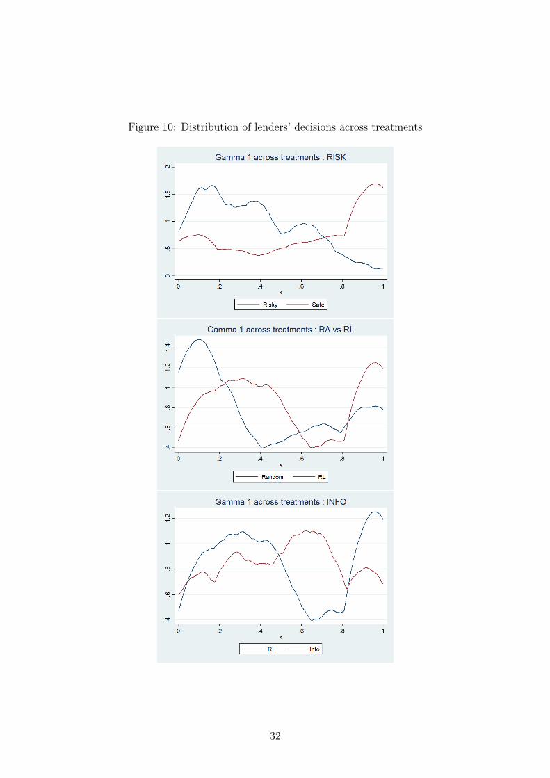
Figure 10: Distribution of lenders’ decisions across treatments

32

Figure 11: Conditional distributions

33

Table 4: Summary statistics: Random treatment

Random - #low Random - #high ttestmean sd mean sd ttest t stat

$ 0.82 0.39 0.96 0.19 0.138** 2.30"1 0.21 0.41 0.57 0.49 0.362*** 13.56"2 0.21 0.41 0.39 0.49 0.178*** 4.89Full choice 0.73 0.44 0.82 0.38 0.0956*** 3.97Avg volume lent 3.36 2.29 7.33 3.86 3.978*** 12.17Avg volume repaid 1.94 4.30 8.01 5.64 6.068*** 20.49Rationed 0.70 0.46 0.27 0.44 0.435*** 9.54n. switches 0.18 0.38 0.06 0.23 0.116*** 3.64* p < 0.10, ** p < 0.05, *** p < 0.01

Table 5: Summary statistics: Relationship Lending treatment

Rel Lend - #low Rel lend - #high ttestmean sd mean sd ttest t stat

$ 0.8 0.40 0.92 0.27 0.121* 1.78"1 0.27 0.44 0.83 0.37 0.565*** 22.76"2 0.16 0.37 0.62 0.49 0.456*** 9.82Full choice 0.68 0.47 0.84 0.36 0.163*** 6.50Avg volume lent 3.33 1.44 9.02 1.36 5.693*** 38.40Avg volume repaid 1.77 1.44 9.74 4.54 7.969*** 29.50Rationed 0.70 0.46 0.13 0.34 0.570*** 13.65n. switches 0.14 0.35 0.06 0.23 0.080*** 2.61* p < 0.10, ** p < 0.05, *** p < 0.01

34

Table 6: Summary statistics: Information Disclosure treatment

Info Disc - #low Info Disc - #high ttestmean sd mean sd ttest t stat

$ 0.75 0.43 0.95 0.21 0.204*** 3.33"1 0.52 0.50 0.62 0.48 0.106*** 3.46"2 0.38 0.49 0.26 0.44 -0.120*** -3.03Full choice 0.75 0.43 0.76 0.42 0.0182 0.68Avg volume lent 6.27 1.27 6.67 3.87 0.409 1.40Avg volume repaid 3 5.04 7.23 5.77 4.230*** 1.52Rationed 0.43 0.50 0.35 0.48 0.080 1.08n. switches 0.15 0.36 0.11 0.31 0.039 1.08* p < 0.10, ** p < 0.05, *** p < 0.01

35

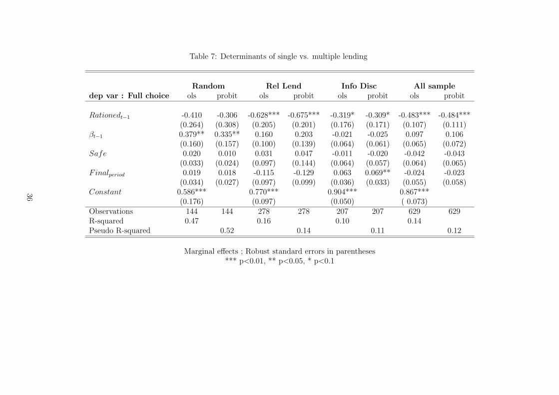
Table 7: Determinants of single vs. multiple lending

Random Rel Lend Info Disc All sampledep var : Full choice ols probit ols probit ols probit ols probit

Rationedt#1 -0.410 -0.306 -0.628*** -0.675*** -0.319* -0.309* -0.483*** -0.484***(0.264) (0.308) (0.205) (0.201) (0.176) (0.171) (0.107) (0.111)

$t#1 0.379** 0.335** 0.160 0.203 -0.021 -0.025 0.097 0.106(0.160) (0.157) (0.100) (0.139) (0.064) (0.061) (0.065) (0.072)

Safe 0.020 0.010 0.031 0.047 -0.011 -0.020 -0.042 -0.043(0.033) (0.024) (0.097) (0.144) (0.064) (0.057) (0.064) (0.065)

Finalperiod 0.019 0.018 -0.115 -0.129 0.063 0.069** -0.024 -0.023(0.034) (0.027) (0.097) (0.099) (0.036) (0.033) (0.055) (0.058)

Constant 0.586*** 0.770*** 0.904*** 0.867***(0.176) (0.097) (0.050) ( 0.073)

Observations 144 144 278 278 207 207 629 629R-squared 0.47 0.16 0.10 0.14Pseudo R-squared 0.52 0.14 0.11 0.12

Marginal e"ects ; Robust standard errors in parentheses*** p<0.01, ** p<0.05, * p<0.1

36

Table 8: Determinants of credit rationing

Random Rel Lend Info Disc All sampledep var : Rationed ols probit ols probit ols probit ols probit

Rationedt#1 0.327 -0.236 -0.020 0.241** 0.551*** 0.095 0.146(0.272) (0.142) (0.017) (0.097) (0.151) (0.079) (0.128)

Rationedt#2 0.320 0.246 0.174** 0.074* 0.448*** 0.481*** 0.445*** 0.429***(0.240) (0.218) (0.060) (0.045) (0.144) (0.164) (0.100) (0.120)

$t#1 -0.008 0.032 -0.486*** -0.672*** -0.263 -0.410** -0.311*** -0.367***(0.090) (0.026) (0.146) (0.146) (0.165) (0.206) (0.104) (0.131)

Full -0.458** -0.992*** -0.653*** -0.764*** -0.224** -0.608*** -0.344*** -0.494***(0.164) (0.008) (0.073) (0.130) (0.082) (0.104) (0.103) (0.131)

Safe 0.000 -0.011 0.018 -0.004 -0.209** -0.357** -0.114* -0.171*(0.059) (0.022) (0.067) (0.046) (0.087) (0.140) (0.066) (0.088)

Finalperiod -0.073 -0.036 -0.015 -0.038 0.130* 0.216** 0.045 0.021(0.050) (0.028) (0.018) (0.024) (0.062) (0.099) (0.037) (0.047)

Constant 0.529** 1.135*** 0.599** 0.737***(0.181) (0.137) (0.208) (0.141)

Observations 135 128 268 268 197 197 600 600R-squared 0.63 0.76 0.66 0.65Pseudo R-squared 0.47 0.78 0.63 0.64

Marginal e"ects ; Robust standard errors in parentheses*** p<0.01, ** p<0.05, * p<0.1

37

Table 9: Determinants of number of switches

Random Rel Lend Info Disc All sampledep. var : n. switches ols ols ols ols

Rationedt#1 10.102*** 5.166*** 3.819*** 6.131***(1.328) (1.271) (0.883) (0.652)

$t#1 -2.509** -2.209** 1.357** -0.404(1.085) (1.040) (0.657) (0.510)

Safe -3.709*** -3.523*** -2.925*** -3.224***(0.638) (0.731) (0.524) (0.355)

Constant 7.402*** 8.466*** 4.612*** 6.056***(1.130) (1.060) (0.554) (0.473)

Observations 144 278 207 629R-squared 0.58 0.19 0.20 0.26

Standard errors in parentheses*** p<0.01, ** p<0.05, * p<0.1

38

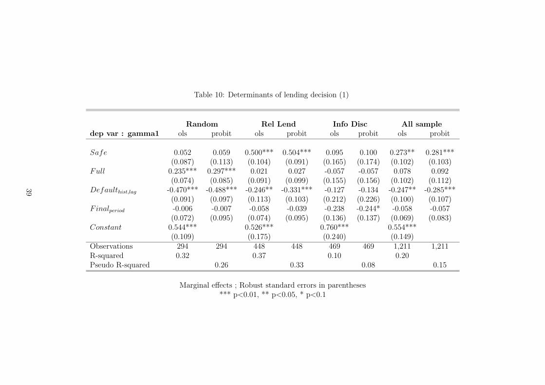
Table 10: Determinants of lending decision (1)

Random Rel Lend Info Disc All sampledep var : gamma1 ols probit ols probit ols probit ols probit

Safe 0.052 0.059 0.500*** 0.504*** 0.095 0.100 0.273** 0.281***(0.087) (0.113) (0.104) (0.091) (0.165) (0.174) (0.102) (0.103)

Full 0.235*** 0.297*** 0.021 0.027 -0.057 -0.057 0.078 0.092(0.074) (0.085) (0.091) (0.099) (0.155) (0.156) (0.102) (0.112)

Defaulthist,lag -0.470*** -0.488*** -0.246** -0.331*** -0.127 -0.134 -0.247** -0.285***(0.091) (0.097) (0.113) (0.103) (0.212) (0.226) (0.100) (0.107)

Finalperiod -0.006 -0.007 -0.058 -0.039 -0.238 -0.244* -0.058 -0.057(0.072) (0.095) (0.074) (0.095) (0.136) (0.137) (0.069) (0.083)

Constant 0.544*** 0.526*** 0.760*** 0.554***(0.109) (0.175) (0.240) (0.149)

Observations 294 294 448 448 469 469 1,211 1,211R-squared 0.32 0.37 0.10 0.20Pseudo R-squared 0.26 0.33 0.08 0.15

Marginal e"ects ; Robust standard errors in parentheses*** p<0.01, ** p<0.05, * p<0.1

39

Table 11: Determinants of lending decision (2, e"ect of being chosen, RL treatment )

dep var : gamma (Model 1) (Model 2) (Model 3) (Model 4)Rel Lend ols probit ols probit ols probit ols probit

Chosen 0.031 0.028 0.050 0.066 0.046 0.058 0.075 0.072(0.042) (0.058) (0.043) (0.060) (0.040) (0.059) (0.095) (0.090)

Lengtht#1 0.039*** 0.059*** 0.015 0.027 0.018* 0.034** 0.011 0.022(0.007) (0.015) (0.009) (0.019) (0.009) (0.016) (0.010) (0.018)

Defaulthist,t#1 -0.381*** -0.491***(0.065) (0.060)

Highdefaultt#1 -0.377*** -0.421***(0.063) (0.077)

Freeridehist,t#1 -0.346*** -0.416***(0.046) (0.062)

$t#1 0.510*** 0.491***(0.125) (0.131)

Safe 0.319*** 0.354*** 0.243*** 0.282*** 0.372*** 0.437*** 0.050 0.057(0.054) (0.057) (0.052) (0.061) (0.046) (0.067) (0.080) (0.088)

Full 0.016 0.026 0.013 0.020 0.003 0.002 0.044 0.049(0.047) (0.062) (0.037) (0.052) (0.043) (0.065) (0.122) (0.120)

Finalperiod -0.100 -0.113 -0.140** -0.178*** -0.073* -0.094* -0.030 -0.032(0.058) (0.081) (0.050) (0.069) (0.039) (0.052) (0.048) (0.052)

Constant 0.630*** 0.648*** 0.502*** 0.223*(0.087) (0.084) (0.068) (0.125)

Observations 444 444 444 444 444 444 209 209R-squared 0.39 0.39 0.41 0.28Pseudo R-squared 0.33 0.31 0.34 0.24

Marginal e"ects ; Robust standard errors in parentheses*** p<0.01, ** p<0.05, * p<0.1

Note : Highdefault,t = 1 if Defaulttt > r

1+r

40

Table 12: Determinants of lending decision (3, e"ect of being chosen, ID treatment )

dep var : gamma (Model 1) (Model 2) (Model 3) (Model 4)Info Disc ols probit ols probit ols probit ols probit

Chosen 0.166*** 0.183*** 0.166*** 0.180*** 0.149** 0.178*** 0.140 0.151(0.052) (0.056) (0.055) (0.059) (0.053) (0.061) (0.097) (0.098)

Lengtht#1 0.048*** 0.076*** 0.045*** 0.075*** 0.032** 0.054*** 0.012* 0.024(0.010) (0.017) (0.012) (0.017) (0.013) (0.021) (0.006) (0.018)

Defaulthist,t#1 -0.170 -0.203(0.183) (0.202)

Highdefaultt#1 -0.167 -0.218(0.132) (0.147)

Freeridehist,t#1 -0.340** -0.368***(0.123) (0.114)

$t#1 0.445*** 0.448***(0.135) (0.145)

Safe -0.095 -0.108 -0.109 -0.134 -0.126 -0.153 0.149 0.164(0.111) (0.128) (0.121) (0.142) (0.087) (0.107) (0.105) (0.105)

Full 0.064 0.080 0.064 0.084 0.080 0.098 0.107 0.134(0.077) (0.087) (0.073) (0.084) (0.080) (0.095) (0.086) (0.093)

Finalperiod -0.216*** -0.230*** -0.236*** -0.249*** -0.121* -0.143** 0.012 0.018(0.064) (0.068) (0.051) (0.056) (0.067) (0.072) (0.069) (0.079)

Constant 0.562*** 0.565*** 0.588*** 0.013(0.174) (0.148) (0.107) (0.160)

Observations 483 483 483 483 483 483 212 212R-squared 0.21 0.22 0.28 0.27Pseudo R-squared 0.18 0.18 0.23 0.23

Marginal e"ects ; Robust standard errors in parentheses*** p<0.01, ** p<0.05, * p<0.1

Note : Highdefault,t = 1 if Defaulttt > r

1+r

41

Table 13: Determinants of being chosen

Rel Lend Info Disc Rel Lend Info Discdep var : Chosen ols probit ols probit ols probit ols probit

"1,t#1 0.254* 0.260* 0.141 0.143 0.089 0.073 -0.012 -0.076(0.132) (0.142) (0.107) (0.107) (0.147) (0.168) (0.107) (0.117)

Safe -0.220 -0.228 -0.130 -0.132 -0.250* -0.260* -0.163 -0.165*(0.139) (0.145) (0.114) (0.114) (0.125) (0.135) (0.098) (0.099)

Finalperiod 0.021 0.024 0.060 0.062 -0.028 -0.027 0.016 0.024(0.067) (0.071) (0.062) (0.064) (0.059) (0.064) (0.058) (0.058)

Lengthfirst,t#1 0.076*** 0.095*** 0.058*** 0.099***(0.022) (0.034) (0.013) (0.029)

Constant 0.419*** 0.456*** 0.457*** 0.500***(0.088) (0.081) (0.078) (0.070)

Observations 294 294 315 315 294 294 315 315R-squared 0.05 0.03 0.13 0.10Pseudo R-squared 0.04 0.02 0.10 0.09

Marginal e"ects ; Robust standard errors in parentheses*** p<0.01, ** p<0.05, * p<0.1

42