June 2010 Q4 a)

Year (Dividend Per Share / Last Year Share Price)

Dividend Yield

2008 38.5 / 740 5.2%

2009 40.0 / 835 4.8%

Year Share Price movement Capital Gain As a Percentage

2008 835 - 740 95c 12.8% (95/740)

2009 648 - 835 -187c -22.4% (-187/835)

Year (capital gain + dividend) / previous year share price

Total Shareholder

Return

Alternative% capital gain + % dividend yield

2008 (95 + 38.5)/740 18.0% 18% (5.2% + 12.8%)

2009 (-187 + 40)/835 -17.6% -17.6% (4.8% - 22.4%)

4 (a) (i) Return on Equity predicted by CAPM

The actual return to a shareholder of QSX Co, calculated as total shareholder return, is different from the return on equity predicted by CAPM.

In 2008, QSX provided a better return than predicted (18% in comparison to 12%) whilst in 2009 the return and CAPM were significantly different (-17.6% to 8%.)

Generally, the return on equity predicted by CAPM will be positive. Shareholders will always want a return to compensate for taking on an investment risk. However as it is an AVERAGE it may well fluctuate.

Companies may on occasion give negative returns, which has happened in this instance.

The return in 2008 was greater than the cost of equity. However, in this example there may be a difference between the current cost of equity and the cost of equity in 2008.

Year Closing Share Price

Earnings per Share

Price/earnings ratio

(Share Price / EPS)

Dividend per share

2007 61.7c 37.0c

2008 $8.35 64.2c 13 times 38.5c

2009 $6.48 58.9c 11 times 40.0c

4 (a) (ii) Other Findings

There has been little growth in turnover for QSX (3% in 2008, 0% in 2009). EPS grew in 2008 (4.1%) but receded in 2009 (-8.3%).

Dividends per share grew by 4.1% in 2008, and this growth was maintained in 2009. Dividends are often maintained when a company experiences financial difficulties to reassure shareholders.

However, most pressing is the issue that the shareholder will experience a capital loss in 2009. A decline in the price/earning ratio in 2009 may be a sign that the market is losing confidence in the QSX Co.

If the shareholder was aware of the planned suspension on dividends then there would be further repercussions.

This information may well remain private and not disclosed to shareholders, However, if QSX wishes to increase its capital due to liquidity issues, these issues will likely become public knowledge relatively quickly through the work of market analysts.

June 2010 Q4 c)

4 (c) Investments, Financing & Dividend Policy

The interlinkage between investments, financing and dividend policy is often referred to as a triangle.

This is because a company is unable to make investments without appropriate financing through debt, equity or the retained earnings within the business.

That financing will also depend on the dividend policy as this will affect retained earnings in the business. In addition, the dividend cannot be paid without successful investments.

Miller & Modigliani suggested that the dividend policy of the firm is irrelevant as the share price of the firm will be dependent on the success of it’s investments.

The optimal use of funds was one that involved investing in all projects with a positive NPV as this would increase shareholder wealth.

The dividend policy of the firm was irrelevant also to shareholders as they would get a return in the form of revenue or capital growth depending on whether dividends were paid.

4 (c) Investments, Financing & Dividend Policy

Miller & Modigliani also suggested that the capital structure of the firm was irrelevant to it’s value as this depended on the business risk rather than the financial risk of the firm.

Business risk is dependent on the industry in which it operates whereas financial risk is the gearing or proportion of debt & equity in the firm.

June 2011 Q3

Financial Analysis 2009 2010 2011

Growth in PBIT -9% -5%

Finance charges growth 10% 4%

Profit for period growth -13% -7%

Interest cover 6.1 5.0 4.6

Payout ratio 55% 64%

EPS (19m Shares) 90.5 78.4 73.1

Price/Earnings Ratio(S. Price / EPS) 5.6 5.9 5.7

Financial Analysis 2009 2010 2011

Dividend per share 50 50

Dividend yield(Divs Per Share / LY S. Price) 8.4% 9.8%

Share price growth -14.1% -10.0% -9.2%

Total Shareholder Return -5.7% -0.2%

Gearing (before debt issue) (50 / 107.5)(50 / 107.5) 47%

Gearing (after debt issue) (100 / 107.5)(100 / 107.5) 93%

3 (a) Financial Performance

The recent results of YNM have been below par. Earnings, net profit and the share price have fallen each year, whilst finance charges have increased year on year.

However, there are positive signs. Despite profits being in a decline, YNM has not made any losses for the past three years.

The rate at which profit has decreased each year has fallen each year. Whilst profit fell 13% in 2010, it only fell 7% in 2011. The rate of growth in finance charges has also reduced, from 10% in 2010 to 4% in 2011.

It could be stated that YNM may be in the process of recovering, which is why the company wishes to seek additional sources of funding to continue its operations.

Financial Position

Interest cover has fallen each year, from 6.1 times in 2009 to 4.6 times in 2011. This ratio has moved away from the comparable ratios of competitors in the same industry (10 times). Also, gearing (47%) is higher than competitors (40%).

Financial risk has increased each year, and YNM’s position is unfavourable in comparison to competitors. Therefore, the issuing of further debt may be dangerous for YNM.

Shareholder Wealth

Some could state that YNM has reduced shareholder wealth due to the continuing fall in its share price. Additionally, a negative total shareholder return in 2010 and 2011 would enhance this claim.

However, due to difficult economic circumstances, it could be stated that YNM has fared better than competitors in reducing the decline in its financial performance.

It maintained the same dividend payment in 2009 and 2010, although this caused the payout ratio to increase from 55% in 2009 to 64% in 2010.

3 (a) (ii) Dividend Choices

YNM has two choices, to pay the same dividend, or to pay no dividend at all.

If YNM decides to pay the same dividend ($9.5m) in 2011, the payout ratio would be similar to 2010 (68%). Total shareholder return would be 1.7% (50 + 417 - 459/459), the first positive number for three years.

Also, the dividend yield would be 11.0% (50/459) which is relatively high. However, paying a $9.5m dividend whilst simultaneously raising $50m of new finance may not be acceptable to debt investors.

If YNM were to pay no dividend in 2011, shareholders would be disappointed. The current cost of equity is 12% and the current share price is $4.17, and through analysis it could be stated that the market is expecting an unchanged dividend (50c/0.12 = $4.17). Paying no dividend would most probably lead to difficulties in raising finance and a fall in YNM’s share price.

By disclosing to the markets the reason for not issuing dividends in 2011 (e.g possibly indicate company plans to increase cash reserves), a fall in the share price could be reduced or prevented.

3 (a) (iii) New debt finance

The current position of YNM would indicate that a new issue of debt would not be successful. If YNM were able to raise $50m worth of debt at the current rate of 8%, gearing would increase to 93% and interest cover would fall to 2.7 times (25.3/(5.5+4)).

In addition, due to the higher risk of taking on this debt, YNM would probably be charged a higher interest rate than 8% and this would compound YNM’s financial position.

YNM would also need to consider the type of finance it wishes to use to raise $50m. Short, medium or long-term finance may be sought, or a combination of different debt types.

The debt would be used to support existing operations, therefore a combination of short-term and long-term finance may be sought. This would give YNM the opportunity to manage interest rate risk by having a short-term variable rate and long-term fixed rate.

However, as YNM is in a poor financial position, other sources of finance should be sought, such as equity finance.

3 (b) (i) - Equity Finance

Equity finance could be raised through a rights issue of shares to existing YNM shareholders, or through a public offer of shares to new shareholders. New equity finance would enhance the gearing ratios of YNM.

However, new and existing shareholders would need to have reassurances from YNM regarding their investments, that company profits will increase in the near future and that the decline in company performance will be stopped as soon as possible.

If equity were raised other than a rights issue, there would be consequences for YNM’s shareholders. If shares were issued at the current share price of $4.17, that would result in the issuance of 12m new shares, a 63% increase. This would dilute the control of existing shareholders, from 100% to 61% ownership.

The level of future dividend payments would also need to be examined. If the current level of dividend payment were to be maintained, this would result in a considerably larger dividend payout than is currently the case.

For instance, if 12m shares were issued, this would result in a total dividend of $15.5m if the dividend per share was 50c.

3 (b) (ii) Sale and Leaseback

Sale and leaseback involves the sale of company owned non-current assets such as land to be sold for cash and leased back for the company’s use. As this would be a long-term transaction, a finance lease would be appropriate.

No further information is provided regarding which of YNM’s non-current assets will be considered, however sale and leaseback has been used to raise larger sums than $50m.

3 (c) Scrip Dividends

A scrip dividend is an alternative to a cash dividend, whereby there is an offer of shares in a company. It is offered pro-rata to current shareholders.

The advantages of scrip dividends include:

Company can retain cash. There is no cash outflow that would arise as a result of a cash dividend. This ensures that cash can be used to either alleviate liquidity issues or to finance other company areas.

Decrease in gearing. The increase in issued shares will increase the company’s equity and consequently reduce the company’s gearing ratio.

Disadvantages of scrip dividends include:

Total dividends will increase. As the number of shares has increased, if the dividend per share is maintained or raised this will result in a higher total cash dividend to shareholders.

December 2009 Q4 b)

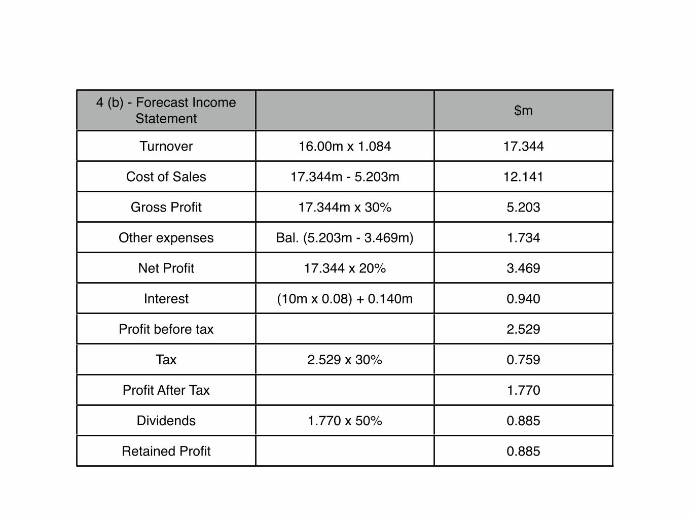
4 (b) - Forecast Income Statement $m

Turnover 16.00m x 1.084 17.344

Cost of Sales 17.344m - 5.203m 12.141

Gross Profit 17.344m x 30% 5.203

Other expenses Bal. (5.203m - 3.469m) 1.734

Net Profit 17.344 x 20% 3.469

Interest (10m x 0.08) + 0.140m 0.940

Profit before tax 2.529

Tax 2.529 x 30% 0.759

Profit After Tax 1.770

Dividends 1.770 x 50% 0.885

Retained Profit 0.885

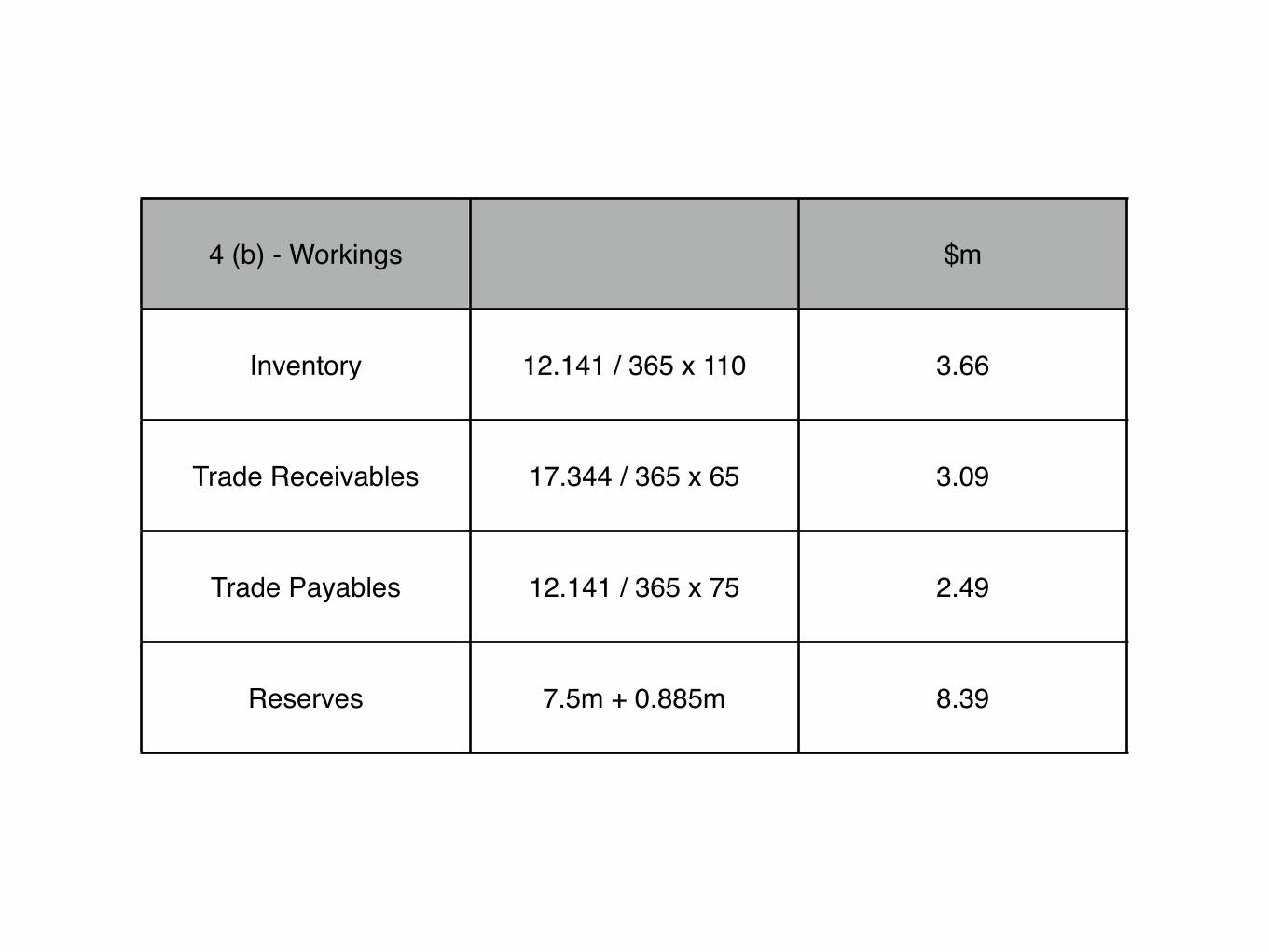
4 (b) - Workings $m

Inventory 12.141 / 365 x 110 3.66

Trade Receivables 17.344 / 365 x 65 3.09

Trade Payables 12.141 / 365 x 75 2.49

Reserves 7.5m + 0.885m 8.39

4 (b) - Forecast Statement of Financial Position $m $m

Non - current assets 22.0

Current assets

Inventory 3.66

Trade receivables 3.09 6.75

Total assets 28.75

Ordinary shares 5.00

Reserves 8.39

13.39

Bank loan 10.00

23.39

Current liabilities

Trade payables 2.49

Overdraft (Bal) 2.87 5.36

Total liabilities 28.75

December 2009 Q4c) + d)

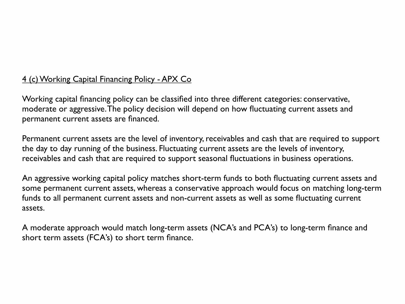
4 (c) Working Capital Financing Policy - APX Co

Working capital financing policy can be classified into three different categories: conservative, moderate or aggressive. The policy decision will depend on how fluctuating current assets and permanent current assets are financed.

Permanent current assets are the level of inventory, receivables and cash that are required to support the day to day running of the business. Fluctuating current assets are the levels of inventory, receivables and cash that are required to support seasonal fluctuations in business operations.

An aggressive working capital policy matches short-term funds to both fluctuating current assets and some permanent current assets, whereas a conservative approach would focus on matching long-term funds to all permanent current assets and non-current assets as well as some fluctuating current assets.

A moderate approach would match long-term assets (NCA’s and PCA’s) to long-term finance and short term assets (FCA’s) to short term finance.

APX currently uses trade payables and an overdraft as sources of short-term finance. 89% (100 x 4.1/4.6) of current assets are funded from short-term sources whereas only 11% are funded from long-term sources.

As a very high proportion of current assets are funded from short-term sources, APX appears to have a very aggressive working capital financing policy. This is a high risk strategy.

The forecast SFP indicates lower levels of short-term finance in the future with 79% (100 x 5·36/6·75) of current assets being funded from short term sources and 21% from long-term sources.

Reducing the aggressive level of working capital policy appears a sensible option. APX could seek future equity investment to reduce its reliance on short-term finance.

4 (d) - Workings $m $m

Turnover 16.00 17.34

Cost of sales 10.88 12.14

Gross Profit 5.12 5.20

Other expenses 1.44 1.73

Net Profit 3.68 3.47

4 (d) - Workings Current Forecast

Gross Profit Margin 100 x 5.12/16.00 32% 30%

Net profit Margin 100 x 3.68/16.00 23% 20%

ROCE 100 x 3.68/22.5 16.35%

100 x 3.469/23.39 14.83%

Inventory period 365 x 2.4/10.88 81 days 110 days

Receivables period 365 x 2.2/16.00 50 days 65 days

Payables Period (365 x 1.9/10.88) 64 days 75 days

Current Ratio (4.6/4.1) 1.12 times

(6.75/5.36) 1.26 times

Quick Ratio (2.2/4.1) 0.54 times

(3.09/5.36) 0.58 times

4 (d) Forecast Financial Performance - APX Co

The working capital ratios of APX will deteriorate over the year. The inventory period is expected to increase by 29 days (110-81), the trade receivables period is expected to increase by 15 days (65-50), and lastly the trade payables period is expected to increase by 11 days (75-64).

This is a cause of concern for APX. APX should compare these forecasts with average industry or sector values to determine the extent of deterioration in comparison to competitors.

Both the current ratio (1.26 times) and the quick ratio (0.58) are expected to increase marginally over the course of the year. Industry sector comparisons would again be useful to compare APX’s performance.

Trade payables and overdraft finance remain relatively static over the period (trade payables 47% in forecast) and short-term finance is expected to fall slightly in the next year.

However, Forecast Gross and Net Profit margins (30% and 20%) are markedly lower than current margins (32% and 23%). This overall deterioration in APX Co’s financial performance must be noted, especially considering turnover is expected to increase over the period.

The deterioration in APX’s working capital performance may be linked to a deterioration of overall financial performance.

June 2008 Q3 d)

3 (d) Working

EOQ √(2 x 6 x 60,000/0.5) 1,200 units

Number of orders (60,000 / 1,200) 50 orders

Annual ordering cost (50 x 6) $300

Average inventory (1,200 / 2) 600 units

Annual holding cost (600 x 0.5) $300

Inventory Cost (60,000 x 12) 720,000

Total Cost of inventory - EOQ (720,000 + 300 + 300) $720,600

3 (d) Working

Order size - bulk discounts 10,000 units

Number of orders (60,000 / 10,000) 6 orders

Annual ordering cost (6 x 6) $36

Average inventory (10,000 / 2) 5,000 units

Annual holding cost (5,000 x 2) $10,000

Discounted material cost (12 x 0.99) $11.88 per unit

Inventory Cost (60,000 x 11.88) 712,800

Total Cost at Discount Level (712,800 + 36 + 10,000) $722,836

December 2010 Q3

3 (a) Current Ordering Policy Working

Order size 10% x 160,000 16,000 units

Number of orders per year 160,000/16,000 10 orders

Annual ordering cost 10 x 400 $4,000

Holding cost ignoring buffer inventory 5.12 x (16,000/2) $40,960

Holding cost of buffer inventory 5.12 x 5,000 $25,600

Total Cost 4,000 + 40,960 + 25,600 $70,560

3 (a)EOQ Model Working

Order size √(2 x 400 x 160,000/5.12) 5,000

Number of orders 160,000/5,000 32 orders

Annual ordering cost 32 x 400 $12,800

Holding cost ignoring buffer inventory 5.12 x (5,000/2) $12,800

Holding cost of buffer inventory 5.12 x 5,000 $25,600

Total Cost using EOQ 12,800 + 12,800 + 25,600 $51,200

Decrease in cost using EOQ model 70,560 - 51,200 $19,360

3 (b) Benefits of JIT

Just-in-time procurement involves the minimisation of inventory held by a company.

The benefits of a JIT procurement policy include:A reduction in holding inventory costs. The company may not have any inventory on its balance sheet, therefore there is no holding cost.

Lower level of investment in working capital. There will be less capital tied up in inventory, allowing the company to allocate capital to other more profitable areas.

Improved supplier relationship, due to the need of a good relationship between both parties to ensure the JIT system will work effectively.

Reduction in material handling costs and improved operating efficiency. Bottlenecks can hopefully be eradicated, therefore ensuring a more efficient production process which will not require material handling costs.

Lower re-production costs. As there is an emphasis on the quality of supplies, hold-ups in the production process will be minimised, ensuring that inventory that is purchased can be fully utilised to create the end product.

3 (c)Changes in Receivables Working

25% customers take discount (87.6 / 365 x 30 x 25%) 1.8

75% customers don’t take discount (87.6 / 365 x 60 x 75%) 10.8

New Receivables 12.6

Current level, trade receivables $18m

Reduction of trade receivables 18 - 12.6 $5.4m

Cost, short-term finance 5.5%

Reduction, finance cost 5.4m x 5.5% $297,000

Admin, operating saving $753,000

Total Benefits $1,050,000

Cost of early settlement discount 87.6m x 0.25 x 0.01 $219,000

Benefit of early settlement discount 1,050,000 - 219,000 $831,000

3 (c) Change in Receivables management

The proposed changes are financially advantageous, and should be accepted. However, it should be noted that the forecast savings in operating and administration costs are a significant factor in this decision, and these savings may not be realised.

Maximum early settlement discount

Maximum early settlement discount = 100 x ($1,050,000 / (0.25 x $87,600,000)) = 4.8%

3 (d) Factors, Working Capital Policy, Trade Receivables

The following factors must be considered:

Amount of capital invested in trade receivables. If there is a lot of capital tied up in trade receivables, then the company may wish to reduce the level of this investment, through tighter controls on credit and by assessing the creditworthiness of clients.

The cost of credit. If the cost of financing receivables is high, there will be pressures to reduce the period over which credit is offered, as well as potentially reducing the amount of credit offered.

Terms offered by competitors. Competitors terms of credit must be carefully monitored, otherwise the company may lose out to competitors who offer more favourable credit terms.

However, the company must also consider where it gains its competitive advantage, and they may possess advantages in other areas (eg. quality) that make them more attractive to potential consumers.

Level of business risk. The level of risk of bad debts to a company will vary depending on a company’s risk appetite.

Some companies may offer more relaxed trade terms to encourage consumer purchases whilst also compensating this with a higher provision for bad debt. Companies may seek to mitigate the risk of bad debt through the use of insurance.

Liquidity. Liquidity may be an issue to a an entity, and a company may choose to factor their receivables to accelerate the payment from customers who purchased with credit.

Expertise. A company may not possess the expertise in monitoring customer creditworthiness or customer accounts, therefore they may choose to outsource its receivables management to a factor.

Pilot Paper Q3

3 (a)Change in Credit Policy Working

Current collection period 30 + 10 40 days

Current accounts receivable 6m / 365 x 40 $657,534

New level of credit sales $6.3m

Accounts receivable after policy change 6,300,000 / 365 x 15 x 30% 77,671

6,300,000 / 365 x 60 x 70% 724,932

Total $802,603

Increase in financing cost (802,603-657,534) x 0.07 10,155

Incremental costs 6.3m x 0.005 31,500

Cost of discount 6.3m x 0.015 x 0.3 28,350

Total Increase in costs 70,005

Contribution from increased sales 6m x 0.05 x 0.6 180,000

Net benefit of policy change 180,000 - 70,005 109,995

The change will increase profitability in Ulnad CoThe change will increase profitability in Ulnad CoThe change will increase profitability in Ulnad Co

3 (b) Working

Daily interest rate 5.11/365 0.014% per day

Variance of cash flows 1,000 x 1,000 $1m per day

Transaction cost $18

Spread 3 x ((0.75 x transaction cost x variance)/interest rate) 1/33 x ((0.75 x transaction cost x variance)/interest rate) 1/3

Spread 3 x((0.75 x 18 x 1m)/0.00014) 1/3 $13,757

Lower limit $7,500

Upper limit 7,500 + 13,757 $21,257

Return point 7,500 + (13,757/3) $12,086

3 (b) Relevance of values, cash management

The Miller-Orr model was designed to aid companies to consider the uncertainties relating to receipts and payment.

The cash balance of Renpec Co varies between the upper and lower limit calculated by the model. When the lower limit is reached, cash is raised by selling short-term securities to raise the cash balance to the return point.

Similarly, if the upper limit is reached, cash is used to buy short-term securities to lower the cash balance to the return point.

The Miller-Orr model ensures that Renpec Co always has a sufficient amount of cash, whilst also ensuring it can earn interest from excess cash holdings.

3 (c) Key areas of Accounts Receivable management

There are four primary ares of accounts receivables management listed below:

Policy formation

An accounts receivables management framework should be produced by a company. Aspects of the framework to consider include establishing terms of trade (eg. period of credit, early settlement discounts?), procedures for checking customer creditworthiness, and establishing procedures when accounts become overdue.

Credit analysis

New customers should be assessed for creditworthiness. Information such as bank references and credit agency reports should be used to check whether credit should be offered to a particular customer. The level of credit analysis may differ between customers due to the amount of credit granted, or the possibility of repeat business.

Credit Controls

A review of outstanding accounts should be carried out on a regular basis to ensure overdue accounts are identified. For example, an aged receivables analysis could be used.

Administrative aspects, such as communication with customers and maintenance of accounting records should be kept to a high standard to ensure that data is kept updated to assist the aged receivables analysis.

Collection of amounts due

A company must have an agreed procedure for handling overdue accounts. This could include personal visits, charging interest on outstanding items, and in the final phase, legal action. The potential benefit of any procedure should outweigh its cost.

3 (d) Key factors, working capital funding policy

Working capital financing policy can be classified into three different categories: conservative, moderate or aggressive. The policy decision will depend on how fluctuating current assets and permanent current assets are financed.

Permanent current assets are the level of inventory, receivables and cash that are required to support the day to day running of the business. Fluctuating current assets are the levels of inventory, receivables and cash that are required to support seasonal fluctuations in business operations.

An aggressive working capital policy matches short-term funds to both fluctuating current assets and some permanent current assets, whereas a conservative approach would focus on matching long-term funds to all permanent current assets and non-current assets as well as some fluctuating current assets.

A conservative approach would be seen as a less risky and less profitable option, whereas an aggressive policy would be seen as a riskier option but with the potential for greater profits.

A moderate approach would match long-term assets (NCA’s and PCA’s) to long-term finance and short term assets (FCA’s) to short term finance.

Generally, long-term debt would have a higher cost of finance than short-term debt, as lenders would wish for a larger compensation for lending for longer periods.

However, long-term debt is viewed as more secure from a company’s perspective as terms are fixed to maturity. In comparison, short-term debt can be due on demand, and may be on less favourable terms.

Other aspects to consider may include organisation size, the risk appetite of management, and previous funding decisions within the organisation.

The size of an organisation may affect its ability to raise different types of finance, for example a small organisation may not be able to raise long-term additional finance.

Also, management attitude to risk will determine whether an aggressive, conservative or moderate approach is used for working capital policy.

June 2011 Q1

1 (a) - Year 1 2 3 4

Sales volume (boxes) 700,000 1,600,000 2,100,000 3,000,000

Selling Price $5 $5 $5 $5

Inflation 1.03 1.032 1.033 1.034

Inflate selling price $5.15 $5.305 $5.464 $5.628

Sales ($000/yr) 3,605 8,488 11,474 16,884

Variable cost per box $2.80 $3.00 $3.00 $3.05

Inflation 1.03 1.032 1.033 1.034

Inflated variable cost $2.884 $3.183 $3.278 $3.433

Variable cost ($000/yr) 2,019 5,093 6,884 10,299

1 2 3 4

Fixed costs ($000) 1,000 1,800 2,800 3,800

Inflation 1.03 1.032 1.033 1.034

Inflated fixed costs ($000) 1,030 1,910 3,060 4,277

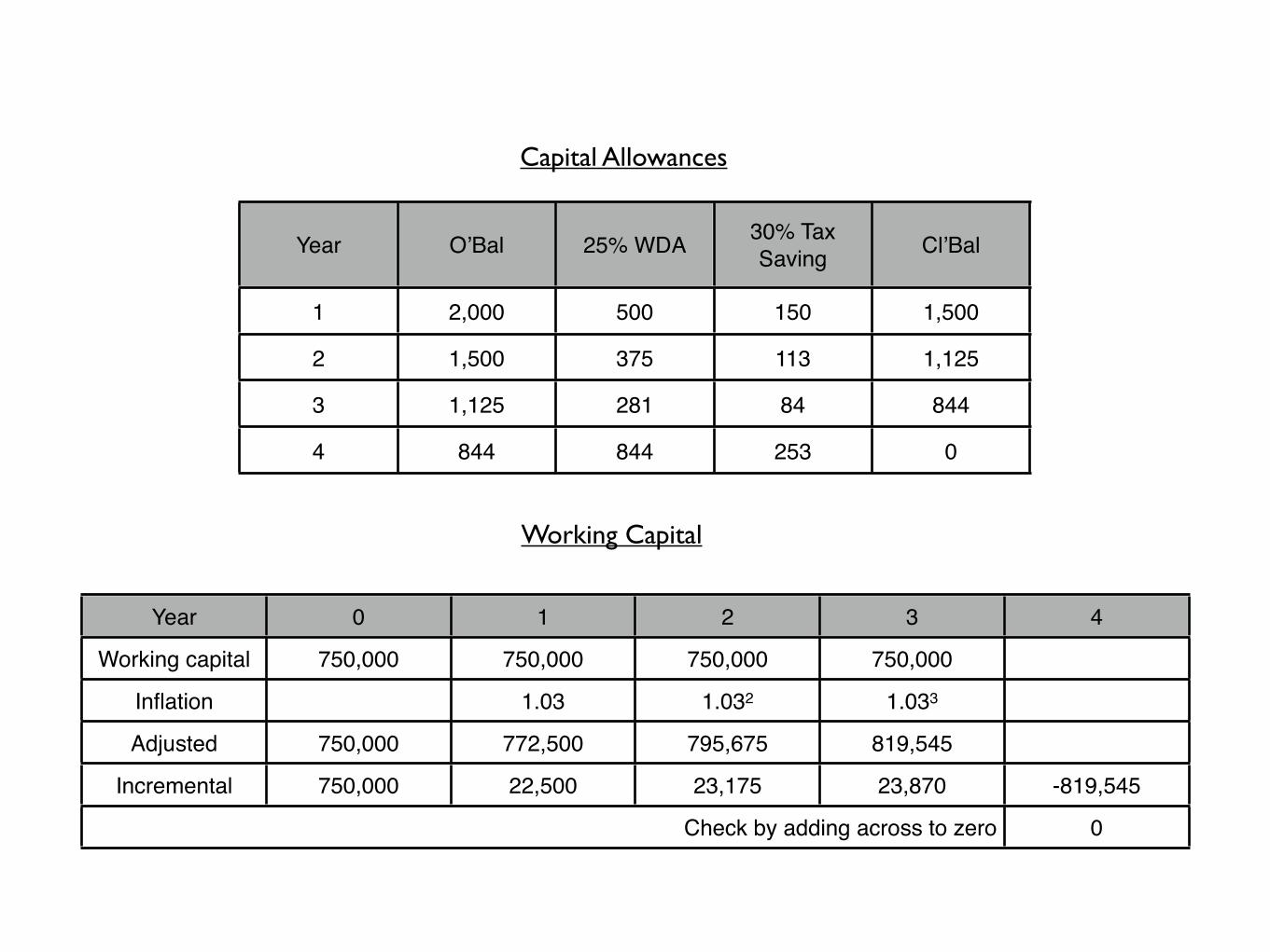
Year O’Bal 25% WDA 30% Tax Saving Cl’Bal

1 2,000 500 150 1,500

2 1,500 375 113 1,125

3 1,125 281 84 844

4 844 844 253 0

Year 0 1 2 3 4

Working capital 750,000 750,000 750,000 750,000

Inflation 1.03 1.032 1.033

Adjusted 750,000 772,500 795,675 819,545

Incremental 750,000 22,500 23,175 23,870 -819,545

Check by adding across to zeroCheck by adding across to zeroCheck by adding across to zeroCheck by adding across to zeroCheck by adding across to zero 0

Capital Allowances

Working Capital

1 (a) - Year 0 1 2 3 4 5

$OOO $OOO $OOO $OOO $OOO $OOO

Sales 3,605 8,488 11,474 16,884

Variable cost -2,019 -5,093 -6,884 -10,299

Fixed costs -1,030 -1,910 -3,060 -4,277

Pre-Tax cash flow 556 1,485 1,530 2,308

Taxation -167 -446 -459 -692

CA tax benefits 150 113 84 253

Initial Investment -2,000

Working Capital -750 -23 -23 -23 820

After-tax cash flow -2,750 533 1,445 1,174 2,753 -439

Discount (12%) 1 0.893 0.797 0.712 0.636 0.567

Present Values -2,750 476 1,152 836 1,751 -249

Net Present Value = $1,215,000, therefore the proposed investment in the new product is acceptable as the NPV is positive.

1 (b) Proposal - four-year time horizon

According to the the finance director, cash flows are too uncertain after four years to be included in the net present value calculation, although sales continue after this point.

Uncertainty does increase over the time of a project, however to cut off the impact of potential sales after the fourth year will underestimate the net present value of the project.

Indeed, estimated high cash flows after the fourth year could significantly enhance the potential investment.

By terminating the value of the investment after the fourth year, the recovery of working capital has been accelerated and there is a large balancing allowance after the fourth year.

These increased cash flows will overestimate the value of the initial investment.

Value of cash flows after the fourth year

Working $

Cash Flows in Year 5 2,308,000

Tax at 30% (2,308,000 x 30%) 692,400

Post Tax Cash Flows 1,615,600

Present Value in Year 4 1,615,600 / 0.12 13,463,333

Discount to get Year 0 PV value 13,463,333 x 0.636 8,562,680

Include 1 year of inflation 1,615,600 x 1.03 / 0.12 13,867,000

Year 0 PV value with 1 year of inflation 13,867,000 x 0.636 8,819,000

Despite the calculations above omitting the capital tax allowance benefits and the investment in working capital, the substantial present value of cash flows show that these should be considered in the initial investment appraisal.

1 (c) Incorporating risk - Investment Appraisal

Risk and uncertainty

Risk can be quantified using probabilities. This enables us to calculate an expected value and use this in our investment appraisal. However, uncertainty cannot be quantified by attaching probabilities. Therefore, the probabilities of risk can be used in an investment appraisal to incorporate risk.

Sensitivity Analysis

A sensitivity analysis is used to calculate the changes in project variables. By altering one variable, it can be used to calculate the change required to make the NPV zero.

Only one variable is considered on each occasion, and once each sensitivity has been calculated, key variables can be identified. These key variables can be the focus of management to ensure that a project will deliver its intended benefits.

However, sensitivity analysis does not include probabilities in its calculation, therefore it cannot be used to incorporate risk into an investment appraisal.

1 (c) Incorporating risk - Investment Appraisal

Probability analysis

Probability analysis assigns probabilities to different values of project variables. A probability analysis can be used to find the worst outcome and its probability (possibly negative NPV), or the best outcome and its probability.

Risk adjusted discount rate

A risk premium would be added to a discount rate to consider a project with greater risk than the norm. Therefore, individual future projects could be compared to assess which one would be the most profitable for the company.

Adjusted payback

By shortening the period of payback, it will reduce the consequent risk. As risk increases over the life-time of a project, reducing the payback period ensures that there is less risk as the period of payback will be less. Payback can also be used by discounting future cash flows using a risk-adjusted rate (discounted payback method.)

June 2009 Q2

2 (a) Key decision - Capital Investment decision-making process

Identify investment opportunities

Investment opportunities can arise from many sources, for example from research & development or the analysis of strategic choices. Most importantly, investment proposals should support the organisations overall objectives.

Screening investment proposals

There will be financial constraints on the amount a company can invest in capital investment. Therefore, companies need to choose between differing investment proposals to select the proposal which is the most appropriate use of resources available.

Analyse and evaluate investment proposals

Possible investment proposals need to be thoroughly scrutinised to evaluate which opportunities most fully match the organisations objectives. Investment appraisal is an important aspect of this stage, and companies will be able to distinguish which projects will deliver the highest net present values.

Approving investment proposals

Investment proposals which are deemed to be the most suitable will be passed onto management for approval. Small proposals may be considered and approved at a divisional level, whereas large proposals may need the approval of the board of directors.

Implementing and monitoring investments

Depending upon the complexity of the project, the project will be implemented, which could take several months. The project must be monitored to ensure that the forecast targets for the project are being attained. In addition, the project should be reviewed to ensure that lessons can be learned for future investment proposals.

1 2 3 4

Selling Price $20 $20 $20 $20

Inflation 1.03 1.032 1.033 1.034

Inflated selling price per unit $20.60 $21.22 $21.85 $22.51

Demand - units per year 60,000 70,000 120,000 45,000

Income per year $1,236,000 $1,485,400 $2,622,000 $1,012,950

Inflation on Sales

2 (b) (i) - Year 1 2 3 4

Variable Cost $8 $8 $8 $8

Inflation 1.04 1.042 1.043 1.044

Inflated variable cost per unit $8.32 $8.65 $9.00 $9.36

Demand - units per year 60,000 70,000 120,000 45,000

Variable costs per year $499,200 $605,500 $1,080,000 $421,200

Fixed Cost $170,000 $170,000 $170,000 $170,000

Inflation 1.04 1.042 1.043 1.044

Inflated fixed costs per year $176,800 $183,872 $191,227 $198,876

Variable costs per year $499,200 $605,500 $1,080,000 $421,200

Operating costs per year $676,000 $789,372 $1,271,227 $620,076

Inflation on Costs

0 1 2 3 4

$ $ $ $ $

Investment -2,000,000

Income 1,236,000 1,485,400 2,622,000 1,012,950

Operating costs -676,000 -789,372 -1,271,227 -620,076

Net cash flow -2,000,000 560,000 696,028 1,350,773 392,874

Discount (10%) 1 0.909 0.826 0.751 0.683

Present values -2,000,000 509,040 574,919 1,014,430 268,333

Net present value $366,722

NPV

2 (b) (ii) - Year 0 1 2 3 4

$ $ $ $ $

Net cash flow -2,000,000 560,000 696,028 1,350,773 392,874

Discount Rate (20%) 1 0.833 0.694 0.579 0.482

Present value -2,000,000 466,480 483,043 782,098 189,365

Net present value -79,014

Internal rate of return 10 + ((366,722 / 366,722 + 79,014) (20 - 10)) = 10 + 8.2 = 18.2%10 + ((366,722 / 366,722 + 79,014) (20 - 10)) = 10 + 8.2 = 18.2%10 + ((366,722 / 366,722 + 79,014) (20 - 10)) = 10 + 8.2 = 18.2%10 + ((366,722 / 366,722 + 79,014) (20 - 10)) = 10 + 8.2 = 18.2%10 + ((366,722 / 366,722 + 79,014) (20 - 10)) = 10 + 8.2 = 18.2%

Internal Rate of Return

2 (b) (iii) Return on Capital Employed

Total cash inflow 560,000 + 696,028 + 1,350,773 + 392,874 $2,999,675

Total depreciation = initial investment there is no scrap value 2,000,000

Total accounting profit 2,999,675 - 2,000,000 $999,675

Average annual accounting profit 999,675 / 4 $249,919

Average investment 2,000,000 / 2 $1,000,000

Return on capital employed 249,919 / 1,000,000 25%

ARR / ROCE

0 1 2 3 4

$ $ $ $ $

PV of cash flows -2,000,000 509,040 574,919 1,014,430 268,333

Cumulative PV -2,000,000 -1,490,960 -916,041 98,389 366,722

Discounted payback period 2 + (916,041/1,014,430) = 2 + 0.9 2 + (916,041/1,014,430) = 2 + 0.9 2 + (916,041/1,014,430) = 2 + 0.9 2 + (916,041/1,014,430) = 2 + 0.9 2.9 years

Discounted Payback

2 (c) Findings

There is a positive NPV for the investment proposal of $366,722, therefore the proposal is financially acceptable.

The IRR method also recommends that the investment is financially acceptable, as the IRR of 18.2% is higher than the 10% return required by PV Co. If the IRR advice differed from that of the NPV, the NPV would still be the preferred method of assessing a proposal.

The ROCE of 25% is less than the target return of 30%. However, the investment proposal is still acceptable as there is a positive NPV. PV Co should assess why it has a target of 30% ROCE, and whether this metric should be updated to meet the current economic climate.

The discounted payback period of 2.9 years accounts for the majority of the investment proposal’s lifecycle. The investment proposal may be sensitive to technological changes, and technological obsolescence may be a factor that could have a significant impact on the financial acceptability of the project.

June 2011 Q2 a) & b)

2 (a) Cost of EquityCost of Equity

Geometric average dividend growth rate

4√(21.8/19.38) - 1 3%

DVM, Ke ((21.8 x 1.03/250) + 0.03 12%

Market values of debt and equityMarket values of debt and equity

Market value, equity 100 x 2.50 $250m

Market value, bonds 60 x (104/100) $62.4m

Total market value 250 + 62.4 $312.4m

Item Market Value Weight Cost Total

Equity 250 (250/312.4) 12 9.60

Bonds 62.4 (62.4/312.4) 7 1.40

312.4 WACC 11.00

Current WACC

Year Cash flow $ 5% Discount PV $ 6%

Discount PV $

Interest Paid = 8 (1-0.3) = 5.6Interest Paid = 8 (1-0.3) = 5.6Interest Paid = 8 (1-0.3) = 5.6Interest Paid = 8 (1-0.3) = 5.6Interest Paid = 8 (1-0.3) = 5.6Interest Paid = 8 (1-0.3) = 5.6Interest Paid = 8 (1-0.3) = 5.61-10 Interest 5.6 7.722 43.24 7.360 41.2210 Capital 105 0.614 64.47 0.558 58.590 Market value -100 1 -100 1 -100

7.71 -0.19

After Tax cost of debtAfter Tax cost of debt 5 + ((6-5) x 7.71)/(7.71 + 0.19))5 + ((6-5) x 7.71)/(7.71 + 0.19))5 + ((6-5) x 7.71)/(7.71 + 0.19)) 5 + 0.98 5.98%

New Bond Issue Kd

2 (a) Revised WACC calculation

The WACC has decreased from 11% to 10.4% due to the increase in the proportion of debt finance. Gearing has increased from 20% (62.4/312.4) to 29%(102.4/352.4).

The WACC makes the assumption that the cost of equity to the company has not changed, however there would be an expectation that the cost of equity would rise due to the increased risk of issuing new debt.

In addition, the share price of the company is assumed to remain constant, which may not happen in reality.

Item Market Value Weight Cost Total

Equity 250 (250/352.4) 12 8.51

Old Bonds 62.4 (62.4/352.4) 7 1.24

New Bonds 40 (40/352.4) 6 0.68

352.4 WACC 10.43

New WACC

2 (b) Factors, Market value of traded bonds

Interest payable

As interest paid on a bond increases, its market value will increase as it becomes more attractive to own the bond.

Frequency of payments

If payments are frequent (eg every six months rather than every year), then the PV of interest payment increases and the market value of the bond increases.

Redemption value

If a value higher than par is offered on redemption, there will be a greater reward for owning the bond, therefore its market value will increase.

Period to redemption

If there is a large period of redemption, this reduces the value of the bond because either the capital payment is paid later than anticipated, or the number of interest payments increases.

Cost of debt

Bond investors wish to obtain a rate of return on their investment. Therefore, the PV of future interest payments are influenced by this cost of debt.

The rate of return is based upon the risk-profile of a company. As the cost of debt decreases, the market value of traded bonds will increase, and vice-versa.

Convertibility

It may be possible to convert bonds into shares, and the market price will be influenced by the likelihood of future conversion. The current share price and future share price growth will need to be considered to assess the market value of the bond.

June 2011 Q2 c)

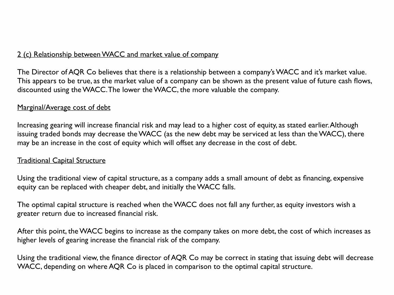
2 (c) Relationship between WACC and market value of company

The Director of AQR Co believes that there is a relationship between a company’s WACC and it’s market value. This appears to be true, as the market value of a company can be shown as the present value of future cash flows, discounted using the WACC. The lower the WACC, the more valuable the company.

Marginal/Average cost of debt

Increasing gearing will increase financial risk and may lead to a higher cost of equity, as stated earlier. Although issuing traded bonds may decrease the WACC (as the new debt may be serviced at less than the WACC), there may be an increase in the cost of equity which will offset any decrease in the cost of debt.

Traditional Capital Structure

Using the traditional view of capital structure, as a company adds a small amount of debt as financing, expensive equity can be replaced with cheaper debt, and initially the WACC falls.

The optimal capital structure is reached when the WACC does not fall any further, as equity investors wish a greater return due to increased financial risk.

After this point, the WACC begins to increase as the company takes on more debt, the cost of which increases as higher levels of gearing increase the financial risk of the company.

Using the traditional view, the finance director of AQR Co may be correct in stating that issuing debt will decrease WACC, depending on where AQR Co is placed in comparison to the optimal capital structure.

Miller & Modigliani

In their first paper, M&M stated that replacing equity with debt did not lead to a decrease in the WACC, as the effect of adding cheaper debt was offset by the increase in the cost of equity.

However, in their second paper M&M described how including the effects of taxation could lead to a decrease in the WACC if equity was replaced with debt. As the interest on debt is tax deductible and thus debt is cheaper, M&M suggested that a company should substitute Equity for Debt in order to take advantage of this fact.

This will also have the effect of increasing the value of the business using the PV of future cash-flows method as the WACC and thus the discount rate will be lower leading to a higher valuation.

Therefore, using M&M’s theory, the issuance of traded bonds would decrease the WACC of AQR Co.

In reality, companies do not add as much debt as possible because of the implications of high gearing on the WACC. Aspects such as bankruptcy costs and the costs to a company of financial distress at high gearing levels were ignored by M & M.

Pecking order

Companies have a preference in terms of different sources of finance, as each will have a different implied cost. The pecking order places sources of finance into the following order of preference: retained earnings, bank loans, ordinary debt, convertible debt and equity.

June 2008 Q1

1 (a) WACCWACC

Cost of Equity 4.7 + (1.2 x 6.5) 12.5%

Cost of convertible debtCost of convertible debtCost of convertible debt

Annual after-tax interest = 7 x (1 - 0.3) = $4.90 per bondAnnual after-tax interest = 7 x (1 - 0.3) = $4.90 per bondAnnual after-tax interest = 7 x (1 - 0.3) = $4.90 per bond

Share price in six years 5.50 x 1.06^6 $7.80

Conversion value 7.80 x 15 $117.00

Conversion is likely, as the conversion value is greater than the par value.Conversion is likely, as the conversion value is greater than the par value.Conversion is likely, as the conversion value is greater than the par value.

Year Cash flow $ 5% Discount PV $ 10%

Discount PV $

Annual after-tax interest = 7 x (1 - 0.3) = $4.90 per bondAnnual after-tax interest = 7 x (1 - 0.3) = $4.90 per bondAnnual after-tax interest = 7 x (1 - 0.3) = $4.90 per bondAnnual after-tax interest = 7 x (1 - 0.3) = $4.90 per bondAnnual after-tax interest = 7 x (1 - 0.3) = $4.90 per bondAnnual after-tax interest = 7 x (1 - 0.3) = $4.90 per bondAnnual after-tax interest = 7 x (1 - 0.3) = $4.90 per bond

1-6 Interest 4.9 5.076 24.87 4.355 21.34

6 Conversion 117.00 0.746 87.28 0.564 66.00

Market valueMarket value -107.11 1 -107.11 1 -107.11

5.04 -19.77

After Tax cost of debtAfter Tax cost of debt 5 + ((5 x 5.04) / (5.04 + 19.77))5 + ((5 x 5.04) / (5.04 + 19.77))5 + ((5 x 5.04) / (5.04 + 19.77))5 + ((5 x 5.04) / (5.04 + 19.77)) 6%

1 (a)

Cost of bank loan 8 x (1 - 0.3) 5.6%

Market value of equity 20m x 5.50 $110m

Market value of convertible debt 29m x 107.11/100 $31.06m

Book value of bank loan $2m

Total market value 110 + 31.06 + 2 $143.06m

Item Market Value Weight Cost Total

Equity 110 (110/143.06) 12.5 9.61

Convertible Bonds 31.06 (31.06/143.10) 6 1.30

Bank Loan 2 (2/143.06) 5.6 0.08

143.06 WACC 10.99

1 (b) WACC used in investment appraisal

If the risks of the investment project are similar to that of the current risks faced by the company, then the WACC can be used as a discount rate in an investment appraisal, as the WACC would reflect these risks.

Where the business risk of an investment is similar to the business risk of continuing operations, the WACC can be used. If the two risks are different, then a project-specific discount rate that includes the business risk of the investment project should be used. The CAPM can be utilised to find the project-specific discount rate.

Where the financial risk of an investment is similar to the financial risks of continuing operations, the WACC can be used. If the two risks are different, then an investment appraisal using the project-specific discount rate should be considered.

A company should also consider the size of the proposed investment and the size of the company. Ideally, the investment should be small in comparison with the overall size of the company. If a company proposes a large investment relative to its size, then the WACC should not be used.

1 (c) Dividend Growth Model/CAPM?

Dividend Growth Model

There are several difficulties in using the dividend growth model as a way of estimating the cost of equity. These are as follows:

Future Dividend growth rate is constant? - The model assumes that the growth rate of dividends will continue into perpetuity, but this is unlikely to be the case. Managers will use previous dividends as a metric for calculating future dividends, however managers will vary the rate of dividends depending on current circumstances.

Estimating future dividend growth rates is very difficult - Trends from historical data can be used to analyse possible future dividends. However, historic data does not take into account current market conditions.

Constant Business Risk? - Using the dividend growth model, there is an assumption that business risk will remain constant, and therefore the cost of equity will remain constant. However, in reality companies are subject to market conditions which can fluctuate, and business risk cannot remain constant in this environment.

CAPM

Using CAPM, all investors are considered to hold diversified portfolios, and consequently only seek a return for the systematic risk of an investment. CAPM will consider the difference between the systematic risk of an individual company and the stock market, and a required rate of return for the investor can be calculated.

This required rate of return can be calculated as the sum of the risk-free rate of return and a risk premium, and this will represent the overall cost of equity. Therefore, there is a link between the systematic risk of a company and it’s cost of equity.

As the CAPM offers a larger degree of certainty due to its use of current and historical data (equity beta, equity risk premium etc), it is suggested that it offers a better estimate of the cost of equity of a company than the dividend growth model.

December 2010 Q1 c)

Project Specific Discount RateProject Specific Discount RateProject Specific Discount Rate

Ungear Proxy Firm Equity Beta βa = 1.5 x (90 / (90 + (30 x 0.7)) 1.22

The first step is to remove the financial risk of the proxy company to leave just the business risk (βa).The first step is to remove the financial risk of the proxy company to leave just the business risk (βa).The first step is to remove the financial risk of the proxy company to leave just the business risk (βa).

Regear with our Financial Risk βe = 1.22 x ((180 + (45 x 0.7)) / 180 1.44

The next step is to regear the βa with the financial risk of CJ Co.The next step is to regear the βa with the financial risk of CJ Co.The next step is to regear the βa with the financial risk of CJ Co.

Fill Into CAPM Ke = 4 + 1.44 (6) 12.64%

To get the project-specific cost of equity we fill the new βe into CAPM.To get the project-specific cost of equity we fill the new βe into CAPM.To get the project-specific cost of equity we fill the new βe into CAPM.

December 2007 Q1

1 (a) (i) Price/Earnings ValuationPrice/Earnings Valuation

EPS of Danoca 40c

Average sector P/E ratio 10

Implied value of ordinary shares of Danoca 40 x 10 $4.00

No of ordinary shares 5 million

Value of Danoca 4.00 x 5m $20 million

1 (a) (ii) Dividend Growth ModelDividend Growth Model

EPS of Danoca 40c

Proposed payout ratio 60%

Proposed dividend of Danoca 40c x 60% 24c per share

If the future dividend growth rate is expected to continue, then the historic dividend growth rate can be used to calculate the expected future

dividend growth rate.

If the future dividend growth rate is expected to continue, then the historic dividend growth rate can be used to calculate the expected future

dividend growth rate.

If the future dividend growth rate is expected to continue, then the historic dividend growth rate can be used to calculate the expected future

dividend growth rate.

Average dividend growth over last two years √(24/22) 4.5%

1 (a)(ii)

Cost of Equity using CAPM 4.6 + 1.4 x (10.6 - 4.6) 13%

Value of ordinary share from dividend growth model

(24 x 1.045) / (0.13 - 0.045) $2.95

Value of Danoca Co 2.95 x 5m $14.75 million

Current market capitalisation ($3.30 x 5m) $16.5 million

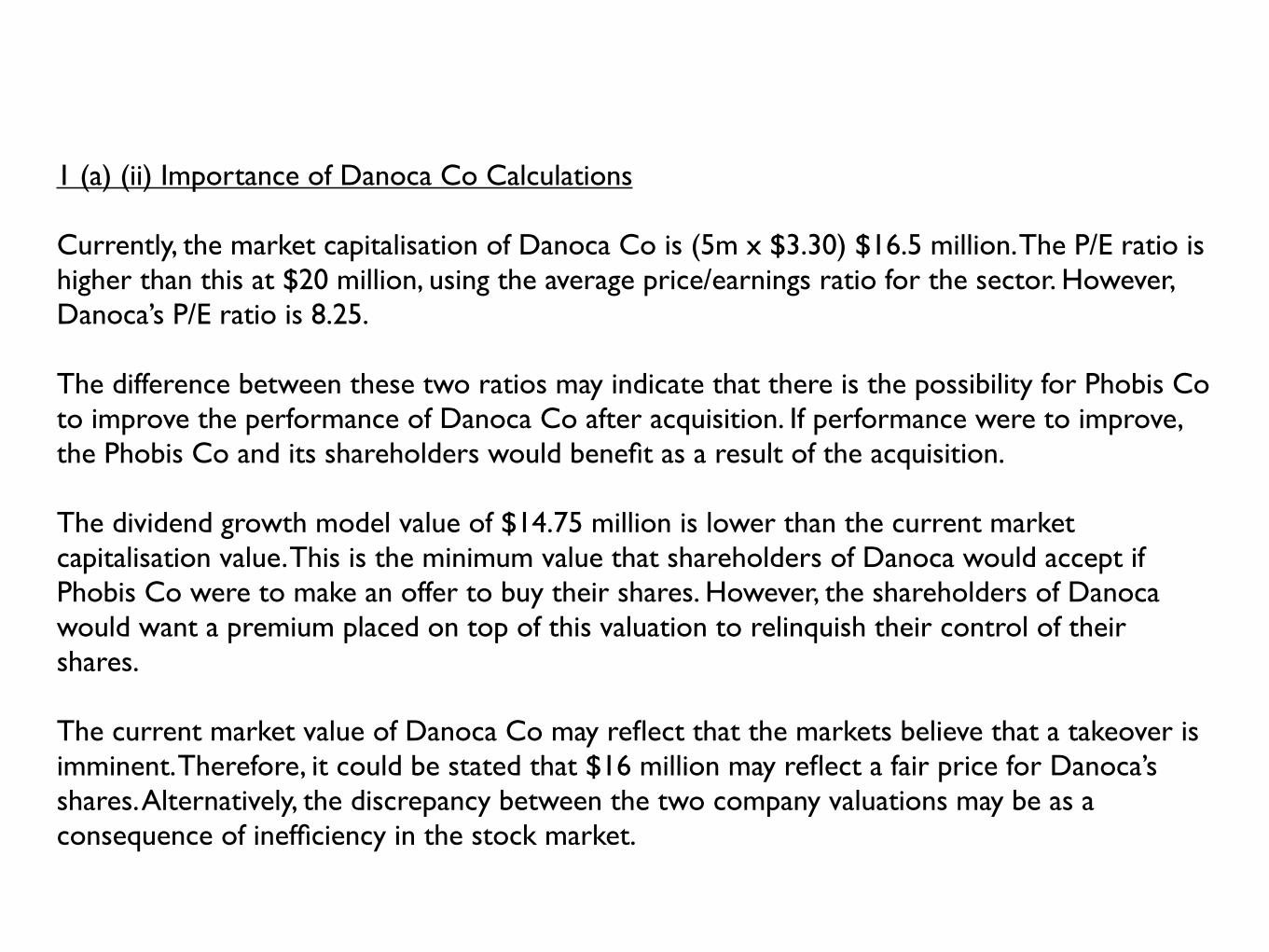
1 (a) (ii) Importance of Danoca Co Calculations

Currently, the market capitalisation of Danoca Co is (5m x $3.30) $16.5 million. The P/E ratio is higher than this at $20 million, using the average price/earnings ratio for the sector. However, Danoca’s P/E ratio is 8.25.

The difference between these two ratios may indicate that there is the possibility for Phobis Co to improve the performance of Danoca Co after acquisition. If performance were to improve, the Phobis Co and its shareholders would benefit as a result of the acquisition.

The dividend growth model value of $14.75 million is lower than the current market capitalisation value. This is the minimum value that shareholders of Danoca would accept if Phobis Co were to make an offer to buy their shares. However, the shareholders of Danoca would want a premium placed on top of this valuation to relinquish their control of their shares.

The current market value of Danoca Co may reflect that the markets believe that a takeover is imminent. Therefore, it could be stated that $16 million may reflect a fair price for Danoca’s shares. Alternatively, the discrepancy between the two company valuations may be as a consequence of inefficiency in the stock market.

Convertible Bond 1 (b)Convertible Bond 1 (b)Convertible Bond 1 (b)

Cash $100

Shares

Current Value $4.45

Value in 5 years with 6.5% growth 4.45 x 1.0655 $6.10

Number of shares per $100 20

Conversion Value 6.10 x 20 $122

Convertible BondPeriod Item $ DR 7% PV

1 - 5 Interest 9 4.1 36.90

5 Conversion Value 122 0.713 86.99

123.89

Floor value -Period Item $ DR 7% PV

1 - 5 Interest 9 4.1 36.90

5 Minimum Redemption 100 0.713 71.30

108.20

Conversion Premium Working Amount

Current Conversion Value 4.45 x 20 89

Expected Value in 5 years (W1) 123.89

Premium 34.89

Premium Per share 34.89 / 20 1.74

1 (c) Weak form, strong-form and semi-strong market efficiency

Stock market efficiency refers to how prices of financial securities reflect relevant information.

Weak-form market efficiency indicates that share prices reflect historic data. Investors, therefore, cannot “beat” the market as the prices only responds to new information that investors do not have.

Semi-strong efficiency indicates that share prices reflect public and historic data. Investors do not gain significant advantage by analysing public information, and the share price will respond quickly to any new information that becomes available to the public.

Strong market efficiency indicates that share prices reflect public and historic data, as well as private information. Investors with access to insider knowledge will not be able to generate substantial returns in this environment. Stock markets are not held as examples of strong market efficiency.

A listed company whose shares are traded on a stock market which is semi-strong form efficient will find that any information relating to the company will be accurately reflected in its share price.

The market will process information quickly and accurately to produce fair prices, therefore managers will not be able to deceive the market. Managers should instead focus on increasing total shareholder wealth.

June 2011 Q4 a)

4 (a)(i) Relationship between exchange rates and interest rates/inflation rates

The relationship between exchange rates and interest rates is referred to as interest rate parity, and the relationship between exchange rates and inflation rates is named purchasing power parity.

Interest rate parity defines the relationship between the interest rates of two countries. The difference between the spot exchange and the forward exchange rate can be linked to the interest rates of each country respectively.

The country which has the highest nominal interest rates will find that it’s currency will weaken in comparison to the country with the lower nominal interest rates. The spot rate and forward rate can be found in the current foreign exchange market.

Purchasing power parity defines the relationship between inflation rates of two countries. The difference between the spot exchange and the forward exchange rate can be linked to the inflation rates of each country respectively.

The country which has the highest inflation rate will find that it’s currency will weaken in comparison to the country with lower inflation rates. Purchasing power parity is used to show that identical items should sell for the same price in different countries, which in turn effects exchange rates.

4 (a) (ii) Forward Market HedgeForward Market Hedge

Interest Payment 5,000,000 pesos

Six-month forward rate for pesos 12.805 pesos per $

Dollar cost of peso interest using forward market 5,000,000 / 12.805 $390,472

4 (a) (ii) Money Market Hedge

Six-month Peso deposit rate 7.5% / 2 3.75%

Pesos deposited Now 5,000,000 / 1.0375 4,819,277 pesos

Number of dollars need to make the transfer now 4,819,277 / 12.500 $385,542

Six-month dollar borrowing rate 4.5% / 2 2.25%

Debt value in six-months time 385,542 x 1.0225 $394,217

The forward market hedge is cheaper by $3,745 ($394,217 - $390,472), therefore it should be used to hedge the peso interest payment.The forward market hedge is cheaper by $3,745 ($394,217 - $390,472), therefore it should be used to hedge the peso interest payment.The forward market hedge is cheaper by $3,745 ($394,217 - $390,472), therefore it should be used to hedge the peso interest payment.

4 (b) (i) Factors that influence working capital policy

Working capital policy involves a framework for managing inventory, trade receivables, cash and trade payables. It sets a framework for a company to be able to decide its level of investment in its current assets and how these assets are to be financed. There are several factors that affect working capital policy:

Nature of Business

As different businesses in different sectors have differing working capital needs, different policies reflecting working capital are necessary for different types of organisations. For example, a supermarket may have low levels of receivables and high levels of inventory, whereas a service company may have high levels of trade receivables and low levels of inventory.

Operating Cycle

Ideally, a company will wish to minimise the amount of working capital finance that it requires. Therefore, a company will wish to manage its operating cycle to ensure that minimal capital finance is required to fund working capital. The company will seek to reduce its inventory and receivables conversion periods and increase its payables deferral period.

Terms of trade

Terms of trade offered by competitors must be analysed so that a company can strategically position itself. For instance, the terms for receivables must be comparable to competitors otherwise the company may lose potential trade from customers.

Risk appetite of company

A risk-taking company may wish to have lower levels of receivables and inventory in comparison to more risk-averse companies.

In addition, risk-taking companies may wish to undertake an aggressive working capital policy by using short-term financing to fund fluctuating current assets and some permanent current assets, whereas risk-averse companies may prefer a more conservative approach by using long-term financing to fund some of its fluctuating assets.

4 (b) (ii) Early Settlement Discount

Annual cost of components 120,000 x 7.50 $900,000 per year

Value of discount offered 900,000 x 0.005 $4,500

Current level of payables 900,000 x 90/365 $221,918

Revised level of payables 900,000 x 30/365 $73,973

Reduction in payables 221,918 - 73,973 $147,945

4 (b) (ii) Early Settlement Discount

Annual cost of borrowing 4.5% per year

Increase in financing cost by taking discount 147,945 x 0.045 $6,657

As the increase in financing cost is $2,157 (6,657 -4,500) higher than the discount offered, ZPS will not benefit from taking the discount offered.As the increase in financing cost is $2,157 (6,657 -4,500) higher than the discount offered, ZPS will not benefit from taking the discount offered.As the increase in financing cost is $2,157 (6,657 -4,500) higher than the discount offered, ZPS will not benefit from taking the discount offered.

4 (b) (ii) Bulk purchase discount

Current number of orders 120,000 / 10,000 12 orders

Current ordering cost 12 x 200 $2,400 per year

Current holding cost (10,000 / 2) x 1 $5,000 per year

Annual cost of components $900,000 per year

Inventory cost under current policy 900,000 + 2,400 + 5,000 $907,400 per year

4 (b) (ii) Bulk purchase discount

Bulk order size to increase to 30,000 components

Number of orders 120,000 / 30,000 4 orders per year

New ordering cost 4 x 200 $800

New holding cost (30,000 / 2) x 2.2 $33,000 per year

Annual cost of components 120,000 x 7.50 x 0.964 $867,600 per year

Inventory cost using discount 867,600 + 800 + 33,000 $901,400 per year

ZPS should accept the bulk order discount as it is financially acceptable, and it saves $6,000 per year (907,400 - 901,400).ZPS should accept the bulk order discount as it is financially acceptable, and it saves $6,000 per year (907,400 - 901,400).ZPS should accept the bulk order discount as it is financially acceptable, and it saves $6,000 per year (907,400 - 901,400).

December 2009 Q1

After-tax cost of borrowing 8.6 x (1 - 0.3) 6% per yearAfter-tax cost of borrowing 8.6 x (1 - 0.3) 6% per yearAfter-tax cost of borrowing 8.6 x (1 - 0.3) 6% per yearAfter-tax cost of borrowing 8.6 x (1 - 0.3) 6% per yearAfter-tax cost of borrowing 8.6 x (1 - 0.3) 6% per year

1 (a) Leasing - Year Cash Flow Amount $ 6% DR Present Value $

0 Lease Rental -380,000 1 -380,000

1-3 Lease Rentals -380,000 2.673 -1,015,740

2-5 Tax savings 114,000 4.212 - 0.943 = 3.269 372,666

PV cost of leasing -1,023,074

O’Bal Capital allowance 25%

Tax benefits30%

2 1,000,000 250,000 75,000

3 750,000 187,500 56,250

4 562,500 140,625 42,188

5 421,875- 100,000 321,875 96,563

0 1 2 3 4 5

Capital -1,000,000 100,000

Licence fee -104,000 -108,160 -112,486 -116,986

Tax Benefits 31,200 32,448 33,746 35,096

WDA Tax benefits 75,000 56,250 42,188 96,563

Net cash flow -1,000,000 -104,000 -1,960 -23,788 58,948 131,659

6% DR 1.000 0.943 0.890 0.840 0.792 0.747

Present Value -1,000,000 -98,072 -1,744 -19,982 46,687 98,349

NPV -974,763

1(b) - Workings - Year 1 2 3 4

Operating cost saving ($ per unit) 6.09 6.39 6.71 7.05

Production (units/year) 60,000 75,000 95,000 80,000

Operating cost savings ($/year) 365,400 479,250 637,450 564,000

Tax liabilities - 30% - ($/year) 109,620 143,775 191,235 169,200

Year 1 2 3 4 5

$ $ $ $ $

Cost savings 365,400 479,250 637,450 564,000

Tax Liabilities -109,620 -143,775 -191,235 -169,200

Net Cash Flow 365,400 369,630 493,675 372,765 -169,200

Discount Rate - 11% 0.901 0.812 0.731 0.659 0.593

Present Values 329,225 300,140 360,876 245,652 -100,336

1 (b) - Evaluation $

Present values of benefits 1,135,557

Present cost of financing -974,762

Net Present value 160,795

The investment is financially acceptable, as it has a positive NPV of $160,795.The investment is financially acceptable, as it has a positive NPV of $160,795.

1 (c) Equivalent Annual Cost/Equivalent Annual Benefit

The equivalent annual cost/annual benefit method is used to calculate the annual cost or benefit over varying lengths of a projects life to find out which length of time is most profitable/cost effective for the business.

A discounted cost of capital is used in the calculation, to distinguish the varying present values and net present values which result from the calculations.

For instance, a net present value of $160,795 was calculated for investing in new technology in (b). The WACC was 11%, with the project life expected to be four years. Therefore, the annuity factor of 11% is 3.102, and the equivalent annual benefit is $51,835.9 per year (160,795/3.102).

If an alternative investment has a lower Economic Annual Benefit than the investment above, then the investment above would still be preferable due to is higher Economic Annual Benefit.

1 (d) Divisible/Non-divisible projects

Capital rationing refers to the fact that companies do not have an unlimited amount of capital available to invest. Therefore, the investment which is most profitable to the company will be undertaken first in comparison with others. However, matters can become more complex on whether projects are divisible or indivisible.

Divisible Projects

In divisible projects, there is an assumption that it is possible to produce a percentage of the whole project. For instance, if 60% of a project were to be implemented, the NPV of the project would be 60% of the total project.

A profitability index can be calculated to assess which projects are the most profitable to the company. This is calculated by dividing the NPV of the project with its initial investment. Therefore, potential projects can be ranked according to their profitability.

Investment funds are placed firstly against the most profitable projects, with a proportion of the final investment being produced if there is sufficient finance.

Indivisible Projects

In indivisible projects, a profitability index will not be able to indicate the best investment schedule as some projects may be indivisible. In this scenario, the NPV of all possible investment project combinations should be calculated. The projects with the highest NPV which are achievable will then be undertaken.

December 2012 Q1

1(a) - Workings - Revenue

Year1 2 3 4

Sales - small houses 15 20 15 5

Sales - large houses 7 8 15 15

Small house selling price $200,000 $200,000 $200,000 $200,000

Large house selling price $350,000 $350,000 $350,000 $350,000

1(a) - Workings - Revenue

Year1 2 3 4

Sales revenue - small houses $3,000,000 $4,000,000 $3,000,000 $1,000,000

Sales revenue - large houses $2,450,000 $2,800,000 $5,250,000 $5,250,000

Total sales revenue $5,450,000 $6,800,000 $8,250,000 $6,250,000

Inflated sales revenue $5,614,000 $7,214,000 $9,015,000 $7,034,000

1(a) - Workings - Variable costs

Year1 2 3 4

Sales - small houses 15 20 15 5

Sales - large houses 7 8 15 15

Small house variable costs $100,000 $100,000 $100,000 $100,000

Large house variable cost $200,000 $200,000 $200,000 $200,000

1(a) - Workings - Variable costs

Year1 2 3 4

Variable cost - small houses $1,500,000 $2,000,000 $1,500,000 $500,000

Variable cost - large houses $1,400,000 $1,600,000 $3,000,000 $3,000,000

Total variable cost $2,900,000 $3,600,000 $4,500,000 $3,500,000

Inflated variable cost $3,031,000 $3,931,000 $5,135,000 $4,174,000

1(a) - Workings - Fixed costs

Year1 2 3 4

Fixed Costs $1,500,000 $1,500,000 $1,500,000 $1,500,000

Inflated fixed costs $1,530,000 $1,561,000 $1,592,000 $1,624,000

1(a) - NPV Calculation

Year0 1 2 3 4 5

Sales Revenue $5,614,000 $7,214,000 $9,015,000 $7,034,000

Variable costs -$3,031,000 -$3,931,000 -$5,135,000 -$4,174,000

Contribution $2,583,000 $3,283,000 $3,880,000 $2,860,000

Fixed Costs -$1,530,000 -$1,561,000 -$1,592,000 -$1,624,000

Before-tax cash flow $1,053,000 $1,722,000 $2,288,000 $1,236,000

1(a) - NPV Calculation

Year0 1 2 3 4 5

Initial Investment -$4,000,000

Tax liability -$316,000 -$517,000 -$686,000 -$371,000

CA tax benefits $300,000 $300,000 $300,000 $300,000

After-tax cash flow -$4,000,000 $1,053,000 $1,706,000 $2,071,000 $850,000 -$71,000

DR 12% 1.00 0.893 0.797 0.712 0.636 0.567

PV -$4,000,000 $940,000 $1,360,000 $1,475,000 $541,000 -$40,000

NPV $276,000 The proposal has a positive net present value of $276,000, therefore it is financially acceptable.

The proposal has a positive net present value of $276,000, therefore it is financially acceptable.

The proposal has a positive net present value of $276,000, therefore it is financially acceptable.

The proposal has a positive net present value of $276,000, therefore it is financially acceptable.

1 (b) Return on Capital Employed $

Total before-tax cash flow 6,299,000

Total depreciation 4,000,000

Total accounting profit 2,299,000

Average annual profit 2,299,000/4 $574,500 per year

Average investment 4,000,000/2 $2,000,000

ROCE 100 x 574,500 / 2,000,000 28.7%

1 (b) Discussion

The ROCE of 28.7% is higher than the target ROCE of 20% of the investing company. Therefore, the investment is financially acceptable to the company. In addition, the investment decision should primarily be made using a discounted cash flow method, such as a net present value (NPV) calculation

1 (c) Increase in interest rates - consequences for BKQ Co

A substantial increase in interest rates for BQK Co and its customers will increase their financing costs. This will affect the discount rate used in the investment appraisal decision-making process.

Customer financing costs

A long-term personal loan is taken by customers to finance their house purchase. A substantial increase in interest rates will increase the borrowing costs of existing BQK Co customers, which will in turn increase the amount of cash they have to pay to purchase one of the houses. These increased payments will also affect potential customers of BQK Co.

BQK financing costs

The cost of servicing BQK’s debt will rise due to the interest rate increase. Consequently, there will be an increase in the WACC. The amount of the increase will depend upon the proportion of debt to equity that BQK possesses.

In addition, the cost of equity will also increase due to an interest rate rise. As companies generally have a greater proportion of equity finance in comparison to debt finance, there will be more of an impact to the WACC due to an increase in the cost of equity.

Capital Investment appraisal process

Due to an increase in the WACC, the NPV of some investment projects may no longer be attractive to BQK company. The WACC will be used by BQK as the discount rate to evaluate investment decisions.

Consequently, the prices of the houses may have to be increased to make the investment proposal more attractive. However, the houses may become more difficult to sell, and there could be reduced volumes of sales.

In addition, due to economic circumstances where interest rates are historically high, many customers may not wish to undertake a long-term financial commitment such as purchasing a house.

Furthermore, the costs from suppliers may increase as they wish to increase their prices due to higher borrowing costs.

December 2012 Q2

2 (a) Net cost/benefit $

Current Receivables 2,466,000

Receivables paying within 30 days 15m x 0.5 x 30/365 616,438

Receivables paying within 45 days 15m x 0.3 x 45/365 554,795

Receivables paying within 60 days 15m x 0.2 x 60/365 493,151

Revised receivables 616,438 + 554,795 + 493,151 $1,664,384

2 (a) Net cost/benefit $

Reduction in Receivables 2,466,000 - 1,664,384 801,616

Reduction in financing cost 801,616 x 0.06 48,097

Cost of discount 15m x 0.5 x 0.01 75,000

Net cost of proposed changes 75,000 - 48,097 26,903

Comment

The changes in trade receivables policy are not financially acceptable.

However, KXP Co will need to investigate why there was generally later payment from customers. Trade terms that are offered are similar to competitors, and potentially KXP Co will need to look at its receivables management.

Also, the analysis does not include the provision for bad debts, and it assumes that there will be constant sales, both of which are unlikely to be the case.

2 (b) Cost of current inventory policy $

Cost of materials 540,000 per year

Annual ordering cost 12 x 150 1,800

Annual holding cost 0.24 x (15,000 / 2) 1,800

Total cost of current inventory policy 540,000 + 1,800 + 1,800 543,600 per year

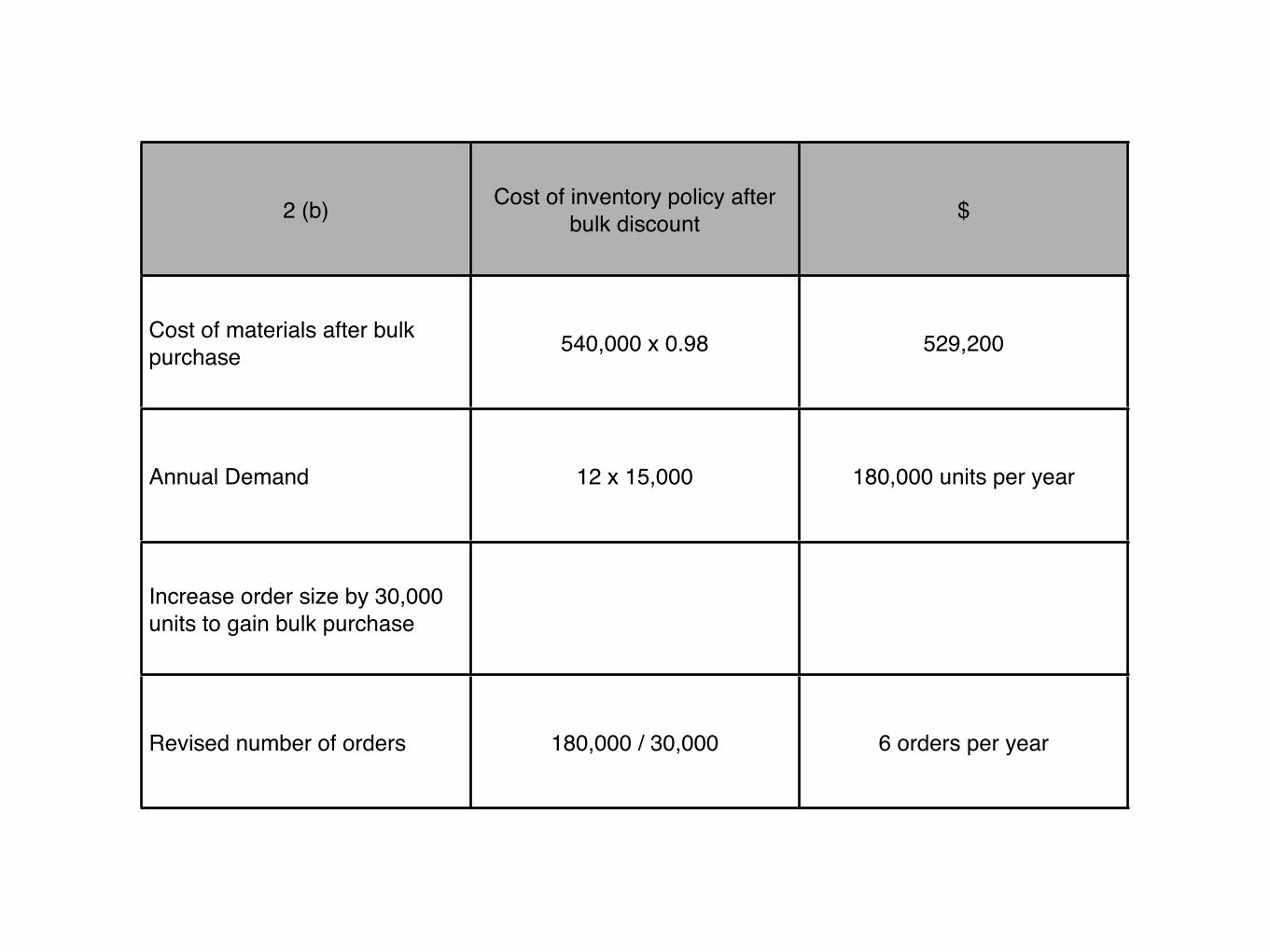
2 (b) Cost of inventory policy after bulk discount $

Cost of materials after bulk purchase 540,000 x 0.98 529,200

Annual Demand 12 x 15,000 180,000 units per year

Increase order size by 30,000 units to gain bulk purchase

Revised number of orders 180,000 / 30,000 6 orders per year

2 (b) Cost of inventory policy after bulk discount $

Revised ordering cost 6 x 150 900 per year

Revised holding cost 0.24 x (30,000 / 2) 3,600 per year

Revised total of inventory policy 529,200 + 900 + 3,600 533,700

Net benefit of bulk purchase discount 543,600 - 533,700 9,900 per year

Comment

The bulk purchase discount appears to be financially acceptable. However, a number of assumptions are included in the analysis. Ordering and holding costs are assumed to be constant throughout, which is unlikely to be the case. Additionally, annual demand is also assumed to be constant, however there will be seasonal fluctuations in demand.

1 (c) Optimum level of cash

Cash required for transactions

One of the three reasons for holding cash is to ensure that you have sufficient funds for future transactions. A forecast for the amount of cash required for the next period will be calculated using a cash budget.

Precautionary need

A cash budget will only offer an estimate for cash needed for transactions, and these estimates are inherently uncertain in nature. In order to provide for an unexpected event, a company can keep a cash buffer to ensure there is cash available to cover an unexpected expense.

The size of the cash buffer will be calculated from historical records, and the company will wish to keep the buffer to a minimum to minimise the opportunity cost of retaining cash funds.

Speculative need

There is a possibility that an investment opportunity may arise and the company may wish to invest. Cash may be made available for this purpose. Additionally, companies may wish to speculate with cash so that they can build up sufficient funds for acquisitions.

Availability of Finance

A company may have difficulty in obtaining finance, for example it may be refused an overdraft facility. Therefore, cash may be required to alleviate their financial issues.

1 (d) Factors - Trade Receivables Policy

Credit Analysis

A company must consider the risk of bad debts and late payments from customers. To lower these risks, a company can assess the creditworthiness of potential customers. The company will require information from a variety of sources, including trade references, bank references and credit reference agencies.

Consequently, the company will be able to assess the potential customer to decide whether they should offer credit and to decide the terms of credit that should be offered to individual customers.

Credit Control

It is important to the company that outstanding credit is paid on time, and that credit limits are not exceeded. Factors may be required to collect funds from overdue accounts. This information can be found using an aged receivables analysis.

Customers will also need to be informed of the outstanding amounts on their accounts and when payment is due. Reminder letters and statements of account can be sent to inform customers of these details.

Receivables Collection

If cash is received through a non-electronic method, it needs to be placed in a bank as soon as possible. Also, steps must be taken to assess overdue accounts, and legal action may be required to recoup outstanding amounts.

The costs of chasing overdue amounts should not exceed the benefits gained from obtaining the overdue funds.

December 2012 Q3

3 (a)

Cost of equity 4 + (1.2 x 5) 10%

Market value of bond 100 x 21m / 20m $105 per bond

Ordinary share price 125m / 25m $5.00 per share

Share price in five years 5.00 x 1.04^5 $6.08

Conversion value 6.08 x 19 $115.52

Conversion is likely to happen, as it is greater than the alternative redemption of $100.Conversion is likely to happen, as it is greater than the alternative redemption of $100.

3 (a) Year Cash flow $ 6% DR PV $ 7% DR PV $

0 Market Price -105.00 1 -105.00 1 -105.00

1-5 Interest 4.90 4.212 20.64 4.100 20.09

5 Conversion 115.52 0.747 86.29 0.713 82.37

1.93 -2.54

Kd 6 + ((7-6) x 1.93) / (1.93 +2.54))6 + ((7-6) x 1.93) / (1.93 +2.54))6 + ((7-6) x 1.93) / (1.93 +2.54)) 6.43%

After-tax interest payment = 0.07 x 100 x (1-0.3) = $4.90 per bond

3 (a)

Cost of preference shares 100 x (0.05 x 10m/6.25m) 8%

Total value of company 125m + 6.25m + 21m $152.25 million

After-tax WACC ((10% x 125m) + (8% x 6.25m) + (6.43% x 21m)) / 152.25m 9.4%

In this instance, the WACC can be ignored in calculating the WACC, even though it is a consistent source of finance for BKB Co.In this instance, the WACC can be ignored in calculating the WACC, even though it is a consistent source of finance for BKB Co.In this instance, the WACC can be ignored in calculating the WACC, even though it is a consistent source of finance for BKB Co.

3 (b) Preference - Market value WACC/ book value WACC

Market values reflect conditions that are currently present in capital markets, whereas book values do not reflect market fluctuations. Therefore, market values are preferred to their book value as they more accurately represent market conditions.

It is important to distinguish the different proportions of finance that a company has in its capital structure, particularly where market values are used as weights. For instance, the market value of equity is generally higher than its book value, therefore there would be an underestimation of the cost of equity if book values were used in its calculation.

This underestimation can be seen in part (a), where the after-tax WACC was calculated as 9.4%, and its relative book value was 8.7% ((10% x 40) + (8% x 10) + (6.43% x 20/70)).

Consequently, if the book value WACC was used as the discount rate for investment appraisals, there would be investment proposals that will be accepted which would otherwise have been rejected if the market value WACC were used instead.

As bonds usually trade on capital markets close to their nominal value, the difference between the book value and market value cost of debt may be minimal, therefore there may be little change in the value of the WACC. However, book values could still under or over-estimate the cost of debt to BKB Co’s WACC.

3 (c) Workings $

Total debt 20m + 15m $35 million

Fixed rate interest 20m x 7% $1.4 million per year

Variable rate interest 15m x 6% $0.9 million per year

Total interest 1.4m + 0.9m $2.3 million

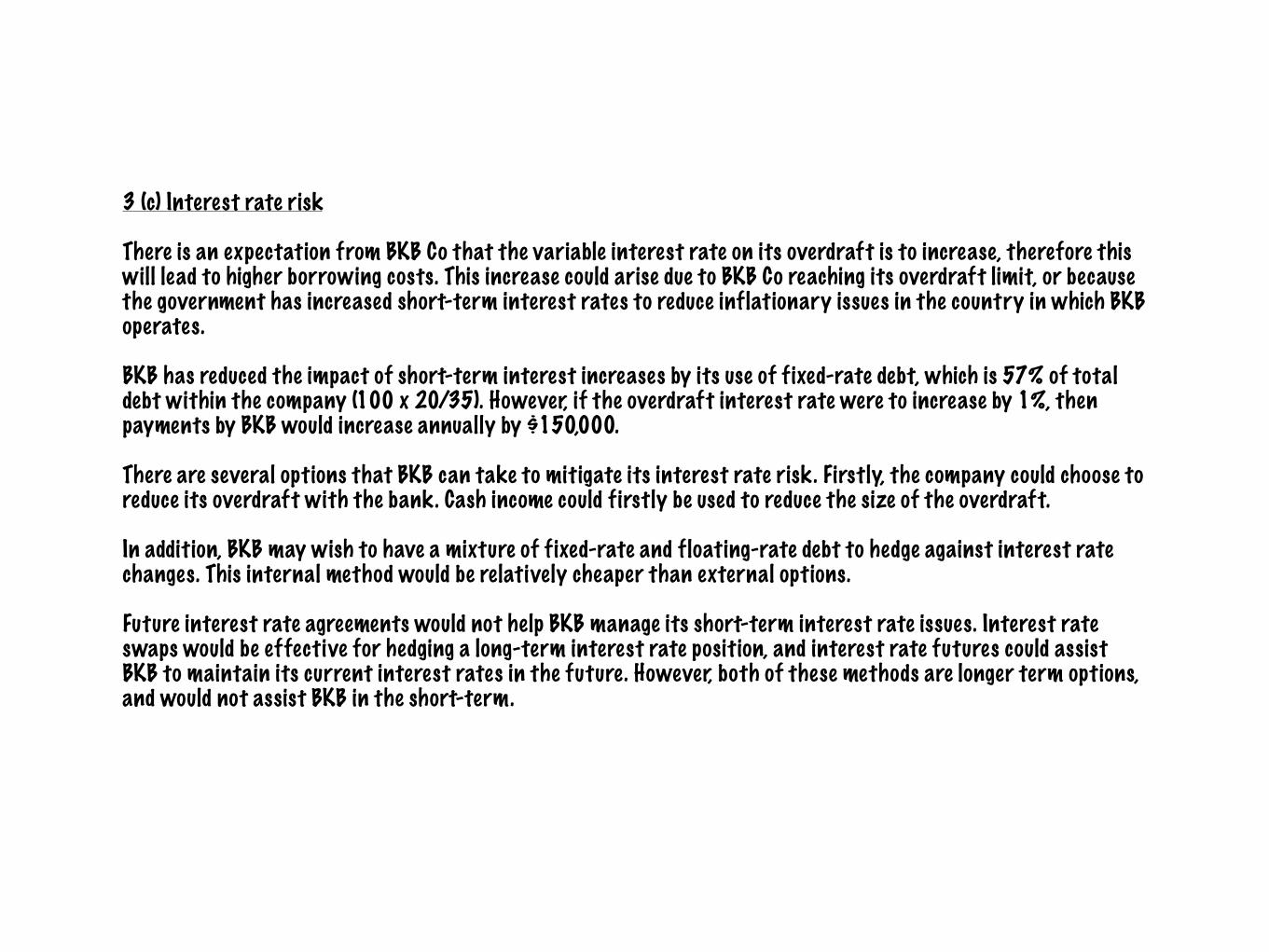
3 (c) Interest rate risk

There is an expectation from BKB Co that the variable interest rate on its overdraft is to increase, therefore this will lead to higher borrowing costs. This increase could arise due to BKB Co reaching its overdraft limit, or because the government has increased short-term interest rates to reduce inflationary issues in the country in which BKB operates.

BKB has reduced the impact of short-term interest increases by its use of fixed-rate debt, which is 57% of total debt within the company (100 x 20/35). However, if the overdraft interest rate were to increase by 1%, then payments by BKB would increase annually by $150,000.

There are several options that BKB can take to mitigate its interest rate risk. Firstly, the company could choose to reduce its overdraft with the bank. Cash income could firstly be used to reduce the size of the overdraft.

In addition, BKB may wish to have a mixture of fixed-rate and floating-rate debt to hedge against interest rate changes. This internal method would be relatively cheaper than external options.

Future interest rate agreements would not help BKB manage its short-term interest rate issues. Interest rate swaps would be effective for hedging a long-term interest rate position, and interest rate futures could assist BKB to maintain its current interest rates in the future. However, both of these methods are longer term options, and would not assist BKB in the short-term.

3 (d) Positives of Convertible debt

Convertible debt gives the holder the option to convert the debt into ordinary shares in the future. If it is not converted, it will retain the characteristics of debt which will be redeemed on maturity. In comparison to a bank loan, convertible debt has the following positive aspects:

Loans not redeemed

Provided that conditions are met, the conversion of convertible debt will be an attractive option to its owners as it is more profitable than redemption. If the debt is converted to ordinary shares, the loan will not need to be redeemed, whereas with a bank loan all of the capital would need to be repaid.

Lower interest rate

In comparison to a bank loan, the interest rate for convertible debt will be lower due to the ability of the bond holders option to convert to shares. Holders of fixed-interest debt will receive a fixed rate of interest from their holding, but they will not be able to increase their returns in line with the success of the company they are lending to.

However, if the debt is converted, the bondholder would benefit from the possibility of higher returns as they are now shareholders.

Reduction in gearing ratio

Gearing is increased when convertible debt is issued. However, if the debt is converted, gearing will fall as the debt proportion has been reduced, and furthermore equity has been used to replace the debt. This ensures that gearing could fall significantly.

Conversion attribute is attractive to investors

Due to the fact that there is the ability to convert debt in the future, this additional characteristic makes convertible debt more attractive to investors. Although short to medium-term prospects may look poor, the ability to convert debt in the future may be particularly attractive to optimistic investors.

December 2012 Q4

4 (a) (i) Market Capitalisation

Value of ordinary shares 20.0 million

Nominal value of ordinary shares 50c

Number of ordinary shares of company 20m / 0.5 40 million shares

Ordinary share price $4.00 per share

Market capitalisation 40m x 4 $160 million

4 (a) (ii) Net Asset value $

Current Net Asset Value 91m + 8.3m - 7.1m - 25m 67.2 million

Decrease in value of NCAs on liquidation 86m - 91m 5 million

Increase in value of inventory on liquidation 4.2m - 3.8m 0.4 million

Decrease in value of receivables 4.5m x 0.2 0.9 million

Net Asset Valuation (liquidation) 67.2m - 5m + 0.4m - 0.9m 61.7 million

4 (a) (iii) Price/earning ratio

Historic earnings of GWW Co $10.1 million

Average PER of GWW Co Business sector 17 times

PER of GWW CO 17 x 10.1m $171.7 million

4 (a) (iv) (1) Dividend Growth model (historic growth rate)

Historic dividend growth rate ((6m / 5m)^0.33 - 1) x 100 6.27%

It is assumed that the future dividend growth is similar to the historic dividend growthIt is assumed that the future dividend growth is similar to the historic dividend growth

Value of GWW CO (6m x 1.0627) / (0.09 - 0.0627) $234 million

4 (a) (iv) (2) Dividend Growth model (Gordon’s growth model)

Gordon’s growth model estimates the dividend growth using g = BReGordon’s growth model estimates the dividend growth using g = BReGordon’s growth model estimates the dividend growth using g = BRe

Historic retention ratio (B) 100 x (3.5 + 3.7 + 4.1 + 4.1) / (8.5 + 8.9 + 9.7 + 10.1) 41%

Current return on shareholders funds (Re) 100 x 10.1 / 67.2 15%

Dividend growth rate 41 x 0.15 6.15%

Value of GWW Co (6m x 1.0615) / (0.09 - 0.0615) $224 million

4 (b) Valuation Methods

Market Capitalisation

Market capitalisation is a way to measure a company’s value by assessing capital markets. However, the share price of a company will fluctuate due to the release of new information, which will in turn affect the market value of the company.

For GWW Co, market capitalistation calculates the minimum value that shareholders can obtain from capital markets. Shareholders will expect to be offered a premium if they are to relinquish ownership of their shares.

Shareholders will use market capitalisation as a method of assessing any offer that is made to them as the valuation is made on a timely basis.

Net Asset value

The liquidation value of GWW Co can be calculated using the net asset valuation method. A reliable measure of the value of the company can be calculated to give shareholders an inclination of the value of the company if it were to be liquidated.

However, this method will often lead to an under-valuation of the company as it will classify the company as a going concern, and few companies will operate with the purpose of becoming liquidated.

Price/Earning ratio

The price/earning ratio is an income based method used to determine a purchase price for a company. Future earnings potential will be used to assess the value of a company.

For GWW Co, earnings for the following year could be calculated as $10.7 million (10.1m x 1.059), using the historic growth rate. Therefore, the price/earning ratio would be $181.9m (17 x 10.7), which is an increase of $10.2 million year-on-year. This increase in value would need to be considered in determining the purchasing price if earnings growth was predicted to continue in the future.

Information which is applicable to the company must be used at all times if it is available. The calculation above for the PER used a sector average, and most likely this would not be an appropriate value to use for GWW Company.

Dividend Growth Model

This model values the company based on the shareholders right to receive future dividends. Therefore, in effect this valuation method is assessing what shareholders would lose if they were to relinquish their ownership of shares in GWW Co.

Similar to market capitalisation, it calculates a minimum value that would be attributed to the purchasing price of a company. However, it must be noted that shareholders do not set dividend policy, where dividends will most likely fluctuate between different periods.

Despite its flaws, the dividend growth model is useful in determining the purchasing price of a company.

4 (c) (i), (ii) + (iii)

(i) Before-tax market value of bonds of GWW (8 x 5.582) + (100 x 0.665) $111.16

(ii) Debt/equity ratio (book value basis) 100 x 25 / 67.2 37.2%

(iii) Debt/equity ratio (market value basis)

Market value of debt 25 x 111.16 / 100 $27.8 million

Market value of equity 4 x 20 / 0.5 $160 million

Debt/equity ratio 100 x 27.8m / 160m 17.4%

4 (c) Usefulness of debt/equity ratio and assessing financial risk

Financial risk is used to describe the variability of returns that a shareholder will receive due to the amount of debt that a company possesses. The debt/equity ratio is a method used to measure the proportion of debt to equity of a company, and in turn this can be used to analyse financial risk. Financial risk will decrease as the debt/equity ratio decreases.

However, the debt/equity ratio requires comparable figures so that it can be adequately assessed. Trends should be noted in the overall composition of debt/equity of a company, with a rising trend indicative of increased financial risk. Also, industry sector average debt/equity ratios can be useful in assessing a company’s financial risk in comparison to its direct competitors.

In addition, the interest cover ratio can be useful in examining financial risk within a company. This ratio can highlight the extent of difficulty that a company may face in making interest payments. A company may experience difficulty in making interest payments even though it may have a low debt/equity ratio.