Jump-and-Rest Effect of U.S. Business Cycles

Jump-and-Rest Effect of U.S. Business Cycles*

Máximo Camacho + Gabriel Perez-Quiros

University of Murcia Banco de España [email protected] [email protected]

Abstract

One of the most familiar empirical stylized facts about output dynamics in the

United States is the positive autocorrelation of output growth. This paper shows that

positive autocorrelation can be better captured by shifts between business cycle states

rather than by the standard view of autoregressive coefficients. The result is extremely

robust to different nonlinear alternative models and applies not only to output but also

to the most relevant macroeconomic variables.

Keywords: Business Cycles, Output Growth, Time Series.

JEL Classification: E32, C22, E27.

* We thank Hugo Rodriguez Mendizabal, the editor, two anonymous referees, and the participants at internal seminar series of the Banco de España, Universidad de Alicante, Universidad Complutense de Madrid, Universidad Autonoma de Madrid and FUNDEAR for helpful comments and suggestions. Maximo Camacho thanks Fundacion BBVA for financial support. Any remaining errors are our own responsibility. The views in this paper are those of the authors and do not represent the views of Bank of Spain or the Eurosystem. + Corresponding Author: Universidad de Murcia, Facultad de Economía y Empresa, Departamento de Métodos Cuantitativos para la Economía, 30100, Murcia, Spain. E-mail: [email protected]

1. Introduction One of the few empirical observations about US output growth dynamics that

is widely accepted in the literature is their positive and significant

autocorrelation. Traditionally, both empirical and theoretical models follow

the standard view that autocorrelation in output is well characterized by

autoregressive processes. At the level of econometric practice, Nelson and

Plosser (1982), Watson (1986), or Campbell and Mankiw (1987) use linear

autoregressive models to document the positive autocorrelation of US output

growth over short horizons. In addition, several authors extend the linear

autoregressive models in order to account for the nonlinear business cycle

behavior of output growth. The papers of Hamilton (1989), Teräsvirta (1995),

and Potter (1995) are significant examples. From the theoretical point of view,

the vast majority of the proposals rely on autoregressive models in order to

check whether the propagation mechanisms induced by their models match

with the observed autocorrelation. Cogley and Nason (1995) include a

comprehensive list of examples.

The purpose of this paper is to provide empirical evidence supportive of an

alternative view of aggregate growth dynamics. In contrast to autoregressive

time series, we show that output growth is better characterized by a recurrent

sequence of shifts between two fixed equilibria of high and low growth means.

On some particular dates that correspond with business cycle turning points,

output growth shows sharp transitions from one regime to the other. However,

within each of these regimes, shocks have no dynamic effect and output

growth fluctuates around state-dependent means as a white noise exhibiting no

conditional autocorrelation. We find that a model with these simple dynamics

is dynamically complete in the sense that further lags of output growth do not

matter in order to explain current growth. This finding is in line with the

results obtained by Kim, Morley and Piger (2005) and Morley and Piger

(2006) in independent works.1

In order to show this fact, we begin our analysis in a simple scenario in

which we assume that the switches between the two states coincide with the

widely accepted record of turning points identified by the National Bureau for

Economic Research (NBER). Under this assumption, we obtain that, once the

NBER business cycle phases are accounted for, the standard autoregressive

parameters are no longer statistically significant and the estimated model is

dynamically complete. In addition, we find that the statistical significance of

the autoregressive parameters falls more when the regime shifts are those

associated with the NBER chronology, as opposed to millions of potential

1 These authors also find that there is no need for autoregressive coefficients in the growth

rates once the nonlinearities are correctly specified. However, their models are more complex

than ours because their purpose is to show the importance of the “third phase” in the business

cycle.

alternative chronologies. This fact provides the NBER sequence with a

“unique” feature never previously found in the literature.

In spite of these findings, we appreciate the limitations in terms of

availability and endogeneity of using the NBER sequence to model the

dynamic specification of output growth. In order to overcome these

limitations, we consider nonlinear extensions to the baseline model that

provide inference of the business cycle shifts without any of the

inconveniences of exogenously considering the location of the NBER turning

points. To ensure that our results are independent of any particular nonlinear

specification, we use a wide range of nonlinear alternatives that are able to

identify sequences of business cycle states which are similar to the NBER

chronology. Significantly, the fact that autoregressive coefficients are not

explicitly needed once these models have accounted for regime switches is

robust to any of them.

To ensure that we are addressing the actual data generating process for

output growth appropriately, we carry out several robustness checks. First, we

check that the absence of autoregressive parameters once we take into account

the business cycle is an intrinsic characteristic of the output growth time series

and not a consequence of the particular sample period selected in the paper or

the last output growth releases. Second, we obtain that the recurrence of

declines and recoveries proposed by the NBER's dating committee is one of

the very few sequences of business cycle dummies which reduce the need for

autoregressive parameters. Third, while we have primarily focused on output

growth, we detect that the absence of autoregressive parameters, after

controlling for the business cycle, has been an important secular regularity

affecting other key macroeconomic aggregates, such as real consumption,

investment, and sales. Finally, we empirically show that simple multiequilibria

models in which the shifts among equilibria are governed by Markov chains

with no autoregressive parameters may be good starting specifications in order

to replicate the main U.S. business cycle characteristics.

This new characterization of output growth (and other economic aggregates)

has several important implications. First, our findings can be interpreted as

empirical evidence in favor of recent developments in theoretical

macroeconomics that explain output dynamics as stochastic switches between

periods of low and high growth with different sources of business cycle

fluctuations. Examples of these papers are Evans, Honkapohja and Romer

(1998), which relies on complementarities among different types of capital

goods, and Azariadis and Smith (1998), where adverse selection problems in

financing capital goods create credit cycles associated with business cycles. In

this context, models with no autoregressive parameters may be useful in

paving the way for further studies along these lines. Second, Cogley and

Nason (1995) pointed out the difficulties that real-business-cycle (RBC)

models have in reproducing the autocorrelation in output growth, and consider

this fact a failure of RBC models. We believe our results may justify the

resuscitation of some of these theoretical models that have been neglected on

the basis of autoregressive parameters as the unique source of the output

growth short-run persistence. Finally, from a technical point of view,

predictions, impulse responses, and dynamic multipliers obtained in nonlinear

contexts become much simpler and more intuitive since they solely rely on our

beliefs about current and future states of the cycle. In addition, the absence of

autoregressive parameters minimizes the mathematical complexity and the

computational cost of simulation and calibration exercises.

The paper is organized as follows. Section 2 outlines the standard and new

stylized facts about the U.S. economy, providing a simple scenario to take

them into account and introducing the main characteristics of the absence of

autoregressive parameters. Section 3 examines the robustness of this new fact

to the sample period, to the business cycle chronology, and to other real

macroeconomic aggregates. Section 4 reveals how the results of the nonlinear

specifications, which generate inferences about business cycle timing,

corroborate the previous findings. Section 5 evaluates the empirical reliability

of our new characterization of output growth. Section 6 concludes.

2. New facts about output growth dynamics

2.1 Stylized facts

The time series literature reports three stylized facts about postwar output

growth dynamics in the United States: output growth is positively

autocorrelated, it exhibits a remarkable business cycle dependence, and its

volatility declined in the mid-eighties. Quotes referring to these facts can be

found throughout the literature, but we can easily appreciate them just by

having a look at the time series. Figure 1 presents these facts for the growth

rate of U.S. real Gross Domestic Product (GDP) for the period 1953.1-2006.4.

In this figure, Chart 1 reports the total and partial sample autocorrelation

functions for output growth, along with the ninety-five confidence bands

( T2± , where T is the sample size). Chart 2 plots the output growth series,

along with several shaded areas that correspond to the NBER recessions, and a

vertical dashed line that refers to 1984.1.2 Finally, Chart 3 shows the kernel

density estimate of output growth before and after the volatility break of

1984.1.

As shown in Chart 1, the pattern of the total sample autocorrelation function

appears to be consistent with the simple geometric decay of first order

autoregressive processes, henceforth AR(1). In addition, the partial

autocorrelation function could be viewed as dying out after one lag, also

consistent with the AR(1) hypothesis with an autoregressive parameter of

about 0.32. This standard result suggests that output growth presents positive

2 This date refers to the structural break in volatility found in Kim and Nelson (1999) and

McConnell and Perez-Quiros (2000).

autocorrelation that could be modeled in specifications that incorporate

autoregressive parameters. This framework is adopted by Cogley and Nason

(1995) to review the standard theoretical real-business-cycle (RBC) models

and to incorporate exogenous sources of dynamics in order to replicate these

impulse dynamics.

Chart 2 and the first column of Table 1 reveal that, while output growth

fluctuates around its mean of 0.80, the broad changes of direction in the series

seem to mark quite well the NBER-referenced business cycles. During

expansions, output growth is usually higher (mean of 1.01) than its

unconditional mean, but declines significantly within recessions (mean of -

0.50). However, these business cycle differences do not seem to affect output

Notes: Shaded areas correspond to the NBER recessions. Dashed line corresponds to the volatility break.

Chart 2. US real GDP growth

-3

0

3

53.2 58.3 63.4 69.1 74.2 79.3 84.4 90.1 95.2 00.3 05.4

-0.2

0

0.2

0.4

1 5 9 13 17 21 25 29 33

-0.2

0

0.2

0.4

1 5 9 13 17 21 25 29 33

Chart 1. Total and partial autocorrelation functions

0

0.5

1

-3.31 -0.81 1.68 4.18

after

before

Figure 1. Stylized facts about US output growth: 1953.1-2006.4

Chart 3. Kernel density estimates growth rates before and after 1984.1

Notes: Shaded areas correspond to the NBER recessions. Dashed line corresponds to the volatility break.

Chart 2. US real GDP growth

-3

0

3

53.2 58.3 63.4 69.1 74.2 79.3 84.4 90.1 95.2 00.3 05.4

-0.2

0

0.2

0.4

1 5 9 13 17 21 25 29 33

-0.2

0

0.2

0.4

1 5 9 13 17 21 25 29 33


0

0.5

1

-3.31 -0.81 1.68 4.18

after

before

0

0.5

1

-3.31 -0.81 1.68 4.18

after

before

Figure 1. Stylized facts about US output growth: 1953.1-2006.4

Chart 3. Kernel density estimates growth rates before and after 1984.1

volatility (standard deviations of 0.73 in expansions and 0.84 in recessions).

Simple tests of the null of no different within-recessions and within-

expansions means and variances are clearly rejected for the means and non

rejected for the variances (p-values of 0.00 and 0.24, respectively).

Finally, Kim and Nelson (1999), and McConnell and Perez-Quiros (2000),

among other authors, have recently detected a substantial moderation in output

growth volatility, with the suggestion that this moderation is well modeled as a

single break in the mid-eighties. We show empirical evidence in favor of this

fact in the first column of Table 1. In particular, we update the supremum,

exponential, and average tests used by McConnell and Perez-Quiros (2000) to

corroborate that 1984.1 is still the more appropriate break date to consider the

structural change in volatility (p-values of 0.00). This fact is also illustrated in

Figure 1 (Chart 3) where, after the break, the distribution of output growth is

clearly more tightly centered on its mean. The results of the Kolmogorov-

Smirnov test and the Wilconxon tests of equality of the quartiles are also

displayed in Table 1, where the null of no change in the distribution of output

growth is clearly rejected. However, contrary to the case of the business cycle,

this break does not seem to affect the mean but the volatility. The former only

moves from 0.81 to 0.77 while the latter falls dramatically from 1.13 to 0.49.

This result is reinforced by the standard tests of no different means and

variances that show p-values of 0.38 and 0.00, respectively.

2.2 A simple approach

To deal with the previous facts about output growth dynamics, a good place to

start is a simple linear autoregressive model. The evidence presented in the

previous section supports a first order process as the best initial candidate. The

first column of Table 2 presents the estimates of this model, labeled as M1,

,110 ttt yaay ε++= − 2.1

where yt represents output growth at time t, and ( )σε ,0~ Nt , which is

identically and independently distributed over time. The estimated

autoregressive coefficient is about 0.32 and generates an endogenous

propagation of impulses that accounts for the positive autocorrelation stated

above. That is to say, the k-period ahead impact of an unanticipated shock is

estimated to be 0.32k. Figure 2 (Chart 1) shows the in-sample fitting of this

model by plotting both the actual and the estimated growth rates. As expected,

after the negative shocks that characterize the peaks, output growth falls

during recessions. However, it is interesting to note that, in all recessions, due

to the smooth dynamics implicit in this autoregressive model, estimates

notably remain above the actual series.

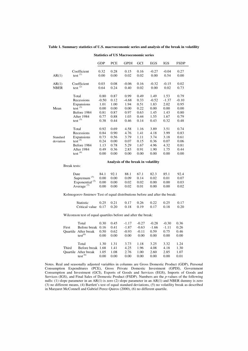
Table 1. Summary statistics of U.S. macroeconomic series and analysis of the break in volatility

Statistics of US Macroeconomic series

GDP PCE GPDI GCI EGS IGS FSDP

Coefficient 0.32 0.28 0.15 0.16 -0.27 -0.04 0.27

AR(1) test (1) 0.00 0.00 0.02 0.02 0.00 0.54 0.00

AR(1) Coefficient 0.03 0.08 -0.06 0.16 -0.32 -0.15 0.02

NBER test (2) 0.64 0.24 0.40 0.02 0.00 0.02 0.73

Total 0.80 0.87 0.99 0.49 1.49 1.53 0.79

Recessions -0.50 0.12 -4.68 0.33 -0.52 -1.37 -0.10

Expansions 1.01 1.00 1.94 0.51 1.83 2.02 0.95

Mean test (3) 0.00 0.00 0.00 0.22 0.00 0.00 0.00

Before 1984 0.81 0.87 0.97 0.63 1.45 1.43 0.80

After 1984 0.77 0.88 1.03 0.44 1.55 1.67 0.79

test (3)

0.38 0.44 0.46 0.14 0.43 0.32 0.48

Total 0.92 0.69 4.58 1.16 3.89 3.51 0.74

Recessions 0.84 0.90 4.76 1.41 4.18 3.99 0.83

Standard Expansions 0.73 0.56 3.79 1.11 3.74 3.18 0.61

deviation test (4) 0.24 0.00 0.07 0.15 0.36 0.07 0.06

Before 1984 1.13 0.78 5.29 1.67 4.96 4.32 0.81

After 1984 0.49 0.36 2.83 0.91 1.90 1.75 0.44

test (4)

0.00 0.00 0.00 0.00 0.00 0.00 0.00

Analysis of the break in volatility Break tests:

Date 84.1 92.1 88.1 67.1 82.3 85.1 92.4

Supremum (5) 0.00 0.00 0.09 0.14 0.02 0.01 0.07

Exponential (5)

0.00 0.00 0.02 0.02 0.00 0.00 0.03

Average (5)

0.00 0.00 0.02 0.01 0.00 0.00 0.02

Kolmogorov-Smirnov Test of equal distributions before and after the break:

Statistic 0.25 0.21 0.17 0.26 0.22 0.25 0.17

Critical value 0.17 0.20 0.18 0.19 0.17 0.18 0.20

Wilconxon test of equal quartiles before and after the break:

Total 0.30 0.45 -1.17 -0.27 -0.28 -0.30 0.36

First Before break 0.16 0.41 -1.87 -0.63 -1.66 -1.11 0.26

Quartile After break 0.50 0.62 -0.93 -0.11 0.59 0.75 0.46

test(6) 0.00 0.00 0.00 0.00 0.00 0.00 0.00

Total 1.30 1.31 3.73 1.18 3.25 3.32 1.24

Third Before break 1.68 1.41 4.25 1.96 4.08 4.18 1.30

Quartile After break 1.05 1.08 2.76 1.00 2.60 2.85 1.07

test (6)

0.00 0.00 0.00 0.00 0.00 0.00 0.01

Notes. Real and seasonally adjusted variables in columns are Gross Domestic Product (GDP), Personal

Consumption Expenditures (PCE), Gross Private Domestic Investment (GPDI), Government

Consumption and Investment (GCI), Exports of Goods and Services (EGS), Imports of Goods and

Services (IGS), and Final Sales of Domestic Product (FSDP). Numbers are the p-values of the following

nulls: (1) slope parameter in an AR(1) is zero (2) slope parameter in an AR(1) and NBER dummy is zero

(3) no different means, (4) Bartlett’s test of equal standard deviations, (5) no volatility break as described

in Margaret McConnell and Gabriel Perez-Quiros (2000), (6) no different quartile.

The simple model in M1 can be easily extended to take into account the

volatility break simply by assuming that ( )ttt BddN 10,0~ +=σε , where Bt

is a dummy that equals one in the period 1984.1-2004.1. The second column

of Table 2, labeled as M2, presents the estimates of this specification. The

estimate of the coefficient d1 is negative and statistically significant, showing

the reduction in volatility of output growth.

2.3. Jump-and-rest effect of business cycles

In this section we look at how business cycle fluctuations influence the

positive autocorrelation of output growth documented in the previous section,

Notes: Shaded areas refer to the NBER recessions. Dashed line corresponds to the volatility break.

Chart 1. Actual versus AR(1)

-3

0

3

53.2 58.3 63.4 69.1 74.2 79.3 84.4 90.1 95.2 00.3 05.4

Figure 2. Output growth estimates: 1953.1-2006.4

-3

0

3

53.2 58.3 63.4 69.1 74.2 79.3 84.4 90.1 95.2 00.3 05.4

-3

0

3

53.2 58.3 63.4 69.1 74.2 79.3 84.4 90.1 95.2 00.3 05.4

Chart 2. Actual versus two-states with volatility break estimates

Chart 3. Actual versus four-states with volatility break estimates


Chart 1. Actual versus AR(1)

-3

0

3

53.2 58.3 63.4 69.1 74.2 79.3 84.4 90.1 95.2 00.3 05.4

Figure 2. Output growth estimates: 1953.1-2006.4

-3

0

3

53.2 58.3 63.4 69.1 74.2 79.3 84.4 90.1 95.2 00.3 05.4

-3

0

3

53.2 58.3 63.4 69.1 74.2 79.3 84.4 90.1 95.2 00.3 05.4

Chart 2. Actual versus two-states with volatility break estimates

Chart 3. Actual versus four-states with volatility break estimates

and its relationship to the standard view of autoregressive coefficients. To

address this question, the simplest way of taking into account the whole set of

stylized facts is by adding a dummy variable to the previous baseline model,

M2, which is equal to one in the NBER recessionary periods.

Table 2. Simple linear time series models of U.S. output growth

M1 M2 M3 M4 M5 M6

a0 0.54 0.54 0.89 0.91 0.91 1.17 (0.08) (0.07) (0.08) (0.04) (0.04) (0.09)

a1 0.32 0.31 0.05 (0.06) (0.06) (0.07)

b0 -1.30 -1.30 -1.31 -1.73 (0.18) (0.14) (0.15) (0.20)

c0 -0.33 (0.10)

c1 0.70 (0.28)

d0 0.87 1.08 0.91 0.92 0.92 0.88 (0.04) (0.07) (0.06) (0.06) (0.06) (0.06)

d1 -0.59 -0.44 -0.46 -0.46 -0.44 (0.08) (0.08) (0.07) (0.07) (0.07)

d2 -0.27 (0.37)

lnL -77.37 -48.02 -23.51 -24.04 -24.01 -18.04

Notes. Entries refer to estimates and standard errors (in parenthesis) that correspond to an

AR(1) for output growth extended with additive and multiplicative dummies that control for

business cycles and volatility break. Last row refers to the log-likelihoods as stated. These

models refer to the following expression:

.,),0(~

,y

210

100110t

ttttt

tttttt

NdBddN

NBcBcNbyaa

++=

+++++= −

σσε

ε

The dummy Bt equals one in the period 1984.1-2006.4, and the dummy Nt equals one in the

NBER periods of recession.

We use Nt to denote the dummy variable that captures the NBER recession

periods. There are many different ways in which the break in the volatility

dummy (Bt) and the NBER dummy (Nt) can modify the previous regressions.

A general characterization of several of these modifications can be

summarized by the following expression:

,100110 ttttttt NBcBcNbyaay ε+++++= − 2.1

where ( )tttt NdBddN 210,0~ ++=σε .3 From this specification, we compute

models M3 to M5 which are generalizations of the standard linear

autoregressive specification with volatility reduction M2.

In model M3 the NBER dates are allowed to interact with the intercept (b0

different from 0). This extension clearly improves the log likelihood function

with respect to M2, which rises from -48.02 to -23.51. Model M3 already

reflects one of the main empirical findings of this paper: once the business

cycle movements of output growth have been taken into account, the

autoregressive parameter is no longer statistically significant. According to

this result, the U.S. economy seems to be characterized by two different steady

states. In the first, the average growth rate of output is positive, while in the

second it is negative. In each of these states, output growth fluctuates around

its mean value as a white noise exhibiting no within-state autocorrelation. The

whole-sample autocorrelation of GDP growth is thus accounted for by the

serial correlation that characterizes the regime switches of the NBER

indicator.

Contrary to the autoregressive processes, in the next period the expected

impact of an unanticipated one-unit increase in current output growth is no

longer one-third. Instead, the impact depends on the date when the shocks

occur. To understand this point, let us take model M4 which, according to the

result of the significance test, imposes on M3 the excluding restriction that the

autoregressive parameter is zero. Now assume the economy is in the negative

growth steady state. For within-recession shocks, the expected impact on

output growth is zero, which is expected to remain at its negative growth state

mean of -0.39. However, shocks occurring in the trough have an expected

instantaneous impact on output growth of 1.30, and zero in subsequent

periods, leading output growth to rise to its positive growth state mean of

0.91.4 Figure 2 (Chart 2) illustrates these dynamics: expected output growth

switches sharply at turning points and remains constant at each steady state

mean until new turning points are reached. This is why we call this particular

effect of business cycles on output growth dynamics the jump-and-rest effect

of business cycles.

Although formal tests are left to Section 5, the charts in Figure 3 enable

useful graphical inspection to investigate the potential serial dependence of

model M4 residuals. Chart 1 plots the residuals time series that seem to follow

the typical erratic pattern of white noise processes. In addition, Chart 2 shows

the total and partial autocorrelation functions of the residuals. They also

support the white noise prior since they show that the autocorrelation at any

lag is not statistically significant.

3 It is worth noting that we failed to obtain any statistically relevant finding from other

variations on the general proposal. 4 We return to this point in the next section in an attempt to provide inference about turning

point identification and a description of the transition between states.

Before concluding this section, we address in Table 2 two additional minor

questions about output growth dynamics. The first has to do with the potential

business cycle dependence of output volatility. To examine this question,

model M5 adds the NBER dummy to the specification of the standard

deviation (d2 different from 0). Following the M5 estimates, we conclude that,

when the volatility break is accounted for, the recessionary dummy does not

affect output volatility (point estimate of -0.27 with standard deviation of

0.37). The second issue deals with the analysis of whether the reduction in

volatility induces a narrower gap in the business cycle means. In this respect,

model M6 includes the volatility dummy in the mean specification (c0 and c1

different from 0). The resulting estimates show that the break significantly

affects the business cycle dynamics (the p-value of joint significance of these

dummies is 0.007). This implies that the volatility reduction may be due to

both a narrowing gap between growth rates during recessions and expansions


Chart 1: residuals

Figure 3. Model M4: residual analysis

-0.2

0

0.2

1 5 9 13 17 21 25 29 33

-0.2

0

0.2

1 5 9 13 17 21 25 29 33


-3

0

3

53.2 58.3 63.4 69.1 74.2 79.3 84.4 90.1 95.2 00.3 05.4


Chart 1: residuals

Figure 3. Model M4: residual analysis

-0.2

0

0.2

1 5 9 13 17 21 25 29 33

-0.2

0

0.2

1 5 9 13 17 21 25 29 33


-3

0

3

53.2 58.3 63.4 69.1 74.2 79.3 84.4 90.1 95.2 00.3 05.4

as in Kim and Nelson (1999), and a decline in output volatility as in

McConnell and Perez-Quiros (2000).5

3. Robustness analysis

In this section we investigate the robustness of the jump-and-rest effect of

business cycles in three different ways. First, we examine whether the absence

of autoregressive parameters when accounting for the business cycle dynamics

is a recent development or whether it is robust to the sample period

considered. Second, we check the extent to which this effect is related to the

particular sequence of business cycles proposed by the NBER. Finally, we

study whether this effect is limited to output growth or shared by other U.S.

major macroeconomic aggregates.

3.1 Is the jump-and-rest effect robust to the sample period?

We have detected that, accounting for the business cycle phases, additional

autoregressive parameters are no longer statistically significant. However, it

would be worth analyzing whether this fact is merely a consequence of the

sample period studied or whether it is rather an intrinsic characteristic of the

output growth dynamics.

This question is addressed in Figure 4 (first row of charts) by using a

recursive approach estimation of output growth. Specifically, we start by

estimating the autoregressive parameter for a short sample spanning 1953.1 to

1963.1. Then, we iteratively expand the initial sample by one observation and

re-estimate the autoregressive parameter in two different scenarios. In the first,

we assume the process to be the simple first-order autoregressive specification

stated in (2.1). Chart 1a shows the OLS estimates of the slope parameter and

Chart 1b plots the p-value of the null of non-significativity. In these graphs,

we observe a secular decrease in the magnitude of the slope parameter while it

constantly remains highly significant. The second scenario modifies the

autoregressive process by the inclusion of the additive NBER-recessionary

dummy variable Nt. Chart 1c shows that, once we allow for business cycle

shifts around turning points, the autoregressive parameter becomes negligible,

and Chart 1d reveals that it has never been statistically significant. These

results confirm that, once business cycle shifts have been accounted for, the

absence of autoregressive parameters in the output growth specification is

robust to the sample period.

5 The output growth mean falls from 1.17 to 0.84 in expansions and rises from -0.56 to -0.19

in recessions after the volatility break. In addition, its standard deviation is reduced from 0.88

to 0.44.

3.2 On the uniqueness of the NBER cycles

So far, we have established that the NBER business cycle fluctuations

represented by a particular sequence of zeroes (expansions) and ones

(recessions) have absorbed and continue to absorb the autocorrelation in

output growth dynamics. An obvious question that arises in the development

of this property is to examine whether this is common to a few or to many

other business cycle sequences, or whether the reduction in the usefulness of

autoregressive parameters to model output growth achieved by the NBER

chronology converts their sequence in “unique” in some sense.

In order to address this question, we propose different exercises. First, we

want to examine to what extent the jump-and-rest effect remains significant

Notes: Computed from rates of growth, Charts labeled with a refer to the recursive estimates of the AR(1) slope

parameters while charts labeled with c refer to the same estimates but obtained by adding a NBER-recessionary

dummy. Charts labeled with b and d refer to their respective p-values of the non-significance null. Horizontal lines

refer to the 0.05 significance value.

0.25

0.35

0.45

63.1 71.4 80.3 89.2 98.1 06.4

Chart1a. Output Chart1b. Output Chart1c. Output Chart1d. Output

Chart2a. Consumption Chart2b. Consumption Chart2c. Consumption Chart2d. Consumption

Chart3a. Investment Chart3b. Investment Chart3c. Investment Chart3d. Investment

Chart4a. Sales Chart4b. Sales Chart4c. Sales Chart4d. Sales

Figure 4. Recursive estimation

AR models AR models with NBER additive dummy

auto

reg

ress

ive

par

am

ete

rsau

tore

gre

ssiv

e p

aram

ete

rsau

tore

gre

ssiv

e p

ara

met

ers

auto

reg

ress

ive

para

mete

rs

auto

reg

ress

ive

para

mete

rsau

tore

gre

ssiv

e p

ara

mete

rsau

tore

gre

ssiv

e p

aram

ete

rsau

tore

gre

ssiv

e p

aram

ete

rs

p-v

alu

esp

-valu

esp

-valu

esp

-valu

es

p-v

alu

esp

-valu

esp

-valu

esp

-valu

es

0

0.06

63.1 71.4 80.3 89.2 98.1 06.4

-0.06

-0.01

0.04

0.09

63.1 71.4 80.3 89.2 98.1 06.4

0

0.5

1

63.1 71.4 80.3 89.2 98.1 06.4

0.25

0.35

0.45

63.1 71.4 80.3 89.2 98.1 06.4

0

0.06

63.1 71.4 80.3 89.2 98.1 06.4

0

0.05

0.1

0.15

63.1 71.4 80.3 89.2 98.1 06.4

0

0.5

1

63.1 71.4 80.3 89.2 98.1 06.4

0.05

0.15

63.1 71.4 80.3 89.2 98.1 06.4

0

0.2

0.4

0.6

63.1 71.4 80.3 89.2 98.1 06.4

-0.3

-0.2

-0.1

0

63.1 71.4 80.3 89.2 98.1 06.4

0

0.3

0.6

63.1 71.4 80.3 89.2 98.1 06.4

0.25

0.35

0.45

63.1 71.4 80.3 89.2 98.1 06.4

0

0.06

63.1 71.4 80.3 89.2 98.1 06.4

-0.03

0.02

0.07

0.12

63.1 71.4 80.3 89.2 98.1 06.4

0

0.5

1

63.1 71.4 80.3 89.2 98.1 06.4

Notes: Computed from rates of growth, Charts labeled with a refer to the recursive estimates of the AR(1) slope

parameters while charts labeled with c refer to the same estimates but obtained by adding a NBER-recessionary

dummy. Charts labeled with b and d refer to their respective p-values of the non-significance null. Horizontal lines

refer to the 0.05 significance value.

0.25

0.35

0.45

63.1 71.4 80.3 89.2 98.1 06.4

Chart1a. Output Chart1b. Output Chart1c. Output Chart1d. Output

Chart2a. Consumption Chart2b. Consumption Chart2c. Consumption Chart2d. Consumption

Chart3a. Investment Chart3b. Investment Chart3c. Investment Chart3d. Investment

Chart4a. Sales Chart4b. Sales Chart4c. Sales Chart4d. Sales

Figure 4. Recursive estimation

AR models AR models with NBER additive dummy

auto

reg

ress

ive

par

am

ete

rsau

tore

gre

ssiv

e p

aram

ete

rsau

tore

gre

ssiv

e p

ara

met

ers

auto

reg

ress

ive

para

mete

rs

auto

reg

ress

ive

para

mete

rsau

tore

gre

ssiv

e p

ara

mete

rsau

tore

gre

ssiv

e p

aram

ete

rsau

tore

gre

ssiv

e p

aram

ete

rs

p-v

alu

esp

-valu

esp

-valu

esp

-valu

es

p-v

alu

esp

-valu

esp

-valu

esp

-valu

es

0

0.06

63.1 71.4 80.3 89.2 98.1 06.4

-0.06

-0.01

0.04

0.09

63.1 71.4 80.3 89.2 98.1 06.4

0

0.5

1

63.1 71.4 80.3 89.2 98.1 06.4

0.25

0.35

0.45

63.1 71.4 80.3 89.2 98.1 06.4

0

0.06

63.1 71.4 80.3 89.2 98.1 06.4

0

0.05

0.1

0.15

63.1 71.4 80.3 89.2 98.1 06.4

0

0.5

1

63.1 71.4 80.3 89.2 98.1 06.4

0.05

0.15

63.1 71.4 80.3 89.2 98.1 06.4

0

0.2

0.4

0.6

63.1 71.4 80.3 89.2 98.1 06.4

-0.3

-0.2

-0.1

0

63.1 71.4 80.3 89.2 98.1 06.4

0

0.3

0.6

63.1 71.4 80.3 89.2 98.1 06.4

0.25

0.35

0.45

63.1 71.4 80.3 89.2 98.1 06.4

0

0.06

63.1 71.4 80.3 89.2 98.1 06.4

-0.03

0.02

0.07

0.12

63.1 71.4 80.3 89.2 98.1 06.4

0

0.5

1

63.1 71.4 80.3 89.2 98.1 06.4

under minor differences in turning point identifications. To do this, we use

leads and lags of the NBER additive dummy as regressors in the OLS

regression of GDP growth rates on an intercept and on its lagged value. That is

to say, we estimate

,1 tititiit NBERyy εγβα +++= −− 3.1

for i=-4,...,0,...,4, where the random error εt is iid normal with mean 0 and

variance σ². In Figure 5, we present the estimated coefficients βi for each

value of i, along with their 95% confidence intervals. As can be seen, only for

i=0 does the coefficient γ0 lead the autoregressive parameter β0 to be

statistically non-significant. All the other values of i other than zero imply

confidence intervals that do not contain the value βi =0. Therefore, minor

differences in turning point identification imply the loss of the jump-and-rest

effect of business cycles.

In a second exercise, we consider how much the absorption of

autocorrelation achieved by the NBER chronology is shared by other business

cycle sequences. This exercise is performed in two scenarios. In the first, we

create business cycle sequences that share the same business cycle properties

as the NBER-dated phases. Here, we generate 10,000 blocks of recessions and

expansions from a Markov process whose probabilities of staying in

expansions, of staying in recessions, and of changing the state give an

expected value of the blocks equal to those observed in the NBER data. With

these 10,000 series of zeroes and ones, we repeat the regressions outlined in

(3.1), where, instead of using NBER leads and lags, we use each of the

generated dummies. The result rejects the null hypothesis that the

Notes: Dashed lines correspond to 95% confidence intervals

Figure 5. Regression with leads and lags of the NBER sequence

-0.2

0

0.2

0.4

0.6

-4 -3 -2 -1 0 1 2 3 4

auto

regre

ssiv

e par

am

eters

Notes: Dashed lines correspond to 95% confidence intervals

Figure 5. Regression with leads and lags of the NBER sequence

-0.2

0

0.2

0.4

0.6

-4 -3 -2 -1 0 1 2 3 4

auto

regre

ssiv

e par

am

eters

autoregressive coefficient is zero in any case. Actually, the minimum value of

the t-statistic is 4.13. In the second scenario, we want to avoid the dependence

of the analysis with respect to the NBER business cycle characteristics. In this

case, we randomly generate 1,000 sets of probabilities of staying in

expansions, staying in recessions, and switching the regime.6 For each of these

vectors of probabilities, we generate 1,000 business cycle dummies and repeat

the previous regression exercise. Remarkably, our result is qualitatively the

same: of the 1,000,000 regressions (i.e., 1,000 vectors of probabilities times

1,000 dummies) the minimum t-statistic of the null that the first order

autoregressive parameter is zero is 3.73. Thus, these results reinforce the idea

that the absorption of autocorrelation is only consistent with some particular

business cycle characteristics associated with the sequence proposed by the

NBER.

Finally, we would like to go even further and try to evaluate the jump-and-

rest effect against all the possible combinations of zeroes and ones. However,

due to the current capacity of our personal computers, the problem seems to be

intractable (217 observations imply 2217

=2.1*1065

possible combinations).7 As

an alternative, we propose an algorithm for seeking a global minimal value in

the autoregressive significance over a huge amount of competing business

cycle dummies, but trying to keep the problem computationally feasible. We

start the algorithm by generating the 65,536 different combinations of

recessions and expansions for the first 16 observations.8 We drop from this set

of possible combinations those that do not have a minimum size block of two

observations (this leaves 19,856 combinations). As usual, we use the

remaining combinations as additive business cycle dummies in the first order

autoregressive regression and keep only those k combinations that provide a p-

value of the null hypothesis of βi=0 (with i=0), which is smaller than or equal

to that obtained using the NBER sequence. We consider that those k selected

business cycle sequences could be followed by an expansion (add one more

zero) or by a recession (add one more one), obtaining 2k business cycle

combinations. With these 2k combinations, we repeat the exercise of

regressing them as dummies in the first order autoregressive time series.

We then continue with this process until we reach the last observation. From

this algorithm we obtain that only one sequence of zeroes and ones reduces the

autocorrelation in the GDP data more than any other sequence of dummies

consistently for most of the samples considered. This sequence is exactly the

same as the NBER recessions dummy, but adding as recession periods the

quarters 1990.3, 1991.2 and 2001.1. Therefore the 1991 recession may start

6 In order to obtain business cycle dummies with economic meaning, we impose that the

probabilities of staying in each state are greater than one half, and that the probability of

staying in expansions is greater than the probability of staying in recessions. 7 In fact, we were able to develop an algorithm that examines the jump-and-rest effect in any

combination of zeroes and ones. However, according to our preliminary results, we would

have required more than 1 year of iterations to finish up the calculations. 8 We tried with different starting sample sizes but they yielded the same results.

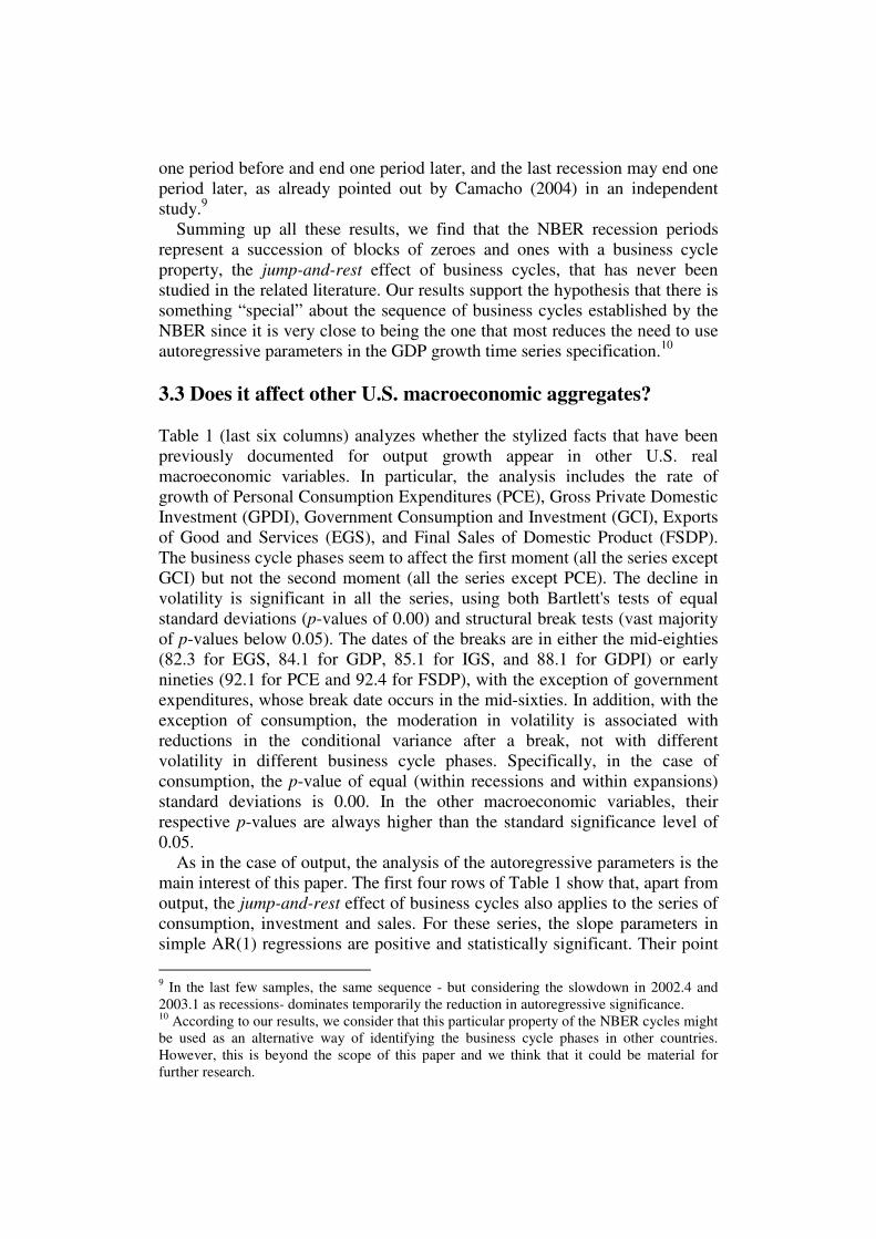
one period before and end one period later, and the last recession may end one

period later, as already pointed out by Camacho (2004) in an independent

study.9

Summing up all these results, we find that the NBER recession periods

represent a succession of blocks of zeroes and ones with a business cycle

property, the jump-and-rest effect of business cycles, that has never been

studied in the related literature. Our results support the hypothesis that there is

something “special” about the sequence of business cycles established by the

NBER since it is very close to being the one that most reduces the need to use

autoregressive parameters in the GDP growth time series specification.10

3.3 Does it affect other U.S. macroeconomic aggregates?

Table 1 (last six columns) analyzes whether the stylized facts that have been

previously documented for output growth appear in other U.S. real

macroeconomic variables. In particular, the analysis includes the rate of

growth of Personal Consumption Expenditures (PCE), Gross Private Domestic

Investment (GPDI), Government Consumption and Investment (GCI), Exports

of Good and Services (EGS), and Final Sales of Domestic Product (FSDP).

The business cycle phases seem to affect the first moment (all the series except

GCI) but not the second moment (all the series except PCE). The decline in

volatility is significant in all the series, using both Bartlett's tests of equal

standard deviations (p-values of 0.00) and structural break tests (vast majority

of p-values below 0.05). The dates of the breaks are in either the mid-eighties

(82.3 for EGS, 84.1 for GDP, 85.1 for IGS, and 88.1 for GDPI) or early

nineties (92.1 for PCE and 92.4 for FSDP), with the exception of government

expenditures, whose break date occurs in the mid-sixties. In addition, with the

exception of consumption, the moderation in volatility is associated with

reductions in the conditional variance after a break, not with different

volatility in different business cycle phases. Specifically, in the case of

consumption, the p-value of equal (within recessions and within expansions)

standard deviations is 0.00. In the other macroeconomic variables, their

respective p-values are always higher than the standard significance level of

0.05.

As in the case of output, the analysis of the autoregressive parameters is the

main interest of this paper. The first four rows of Table 1 show that, apart from

output, the jump-and-rest effect of business cycles also applies to the series of

consumption, investment and sales. For these series, the slope parameters in

simple AR(1) regressions are positive and statistically significant. Their point

9 In the last few samples, the same sequence - but considering the slowdown in 2002.4 and

2003.1 as recessions- dominates temporarily the reduction in autoregressive significance. 10

According to our results, we consider that this particular property of the NBER cycles might

be used as an alternative way of identifying the business cycle phases in other countries.

However, this is beyond the scope of this paper and we think that it could be material for

further research.

estimates are 0.28, 0.15 and 0.17, and their p-values are 0.00, 0.02, and 0.00,

respectively. However, they become negligible and statistically insignificant

when the additive NBER dummy is introduced into their respective baseline

first order autoregressive processes. Specifically, their point estimates become

0.08, -0.06, and 0.02, and their p-values increase to 0.24, 0.40, and 0.73,

respectively.

Finally, as documented in Figure 4, this empirical fact seems to be very

robust to the sample period considered. The secular reduction of the

autoregressive parameters is shared by consumption and sales growth but they

are always highly statistically significant. However, once the NBER business

cycle phases are accounted for, the magnitudes of these parameters are

dramatically reduced and never statistically significant. The case of investment

is somehow special because, even though the jump-and-rest effect of business

cycles has affected its dynamics since the mid-eighties, the slope parameter in

a simple autoregressive regression is not statistically significant for series that

end prior to these years.

4. Nonlinear models of output growth

Although we have found evidence in favor of the two-states model in

contrast to the standard view of autoregressive parameters, the scenario

proposed to develop the analysis was too simple and had limited empirical

application. In particular, we assumed we would observe the discrete shifts

between states directly since we used the dichotomous NBER variable as

known at each time period. In real time, the NBER dating committee

introduces delays in the reporting of the index of up to two years. Moreover,

this model fails to capture the fact that the economies can recover on their own

since the way that the economy leaves a regime depends almost entirely on the

NBER indicator that has been exogenously defined. Finally, using the NBER

indicator as an explanatory variable may lead to potential endogeneity

problems since the indicator has been constructed on the basis of knowing the

actual value for output growth.

We overcome these two problems by using nonlinear extensions to the

baseline model presented in the previous section. These specifications are

useful because they provide inference about the probability of business cycle

shifts in each period with information available up to that period. Furthermore,

they allow us to correct the endogeneity problem that may affect the

estimations of the previous section. Finally, we show that the main

conclusions of this study are invariant to the wide range of nonlinear

specifications that we propose to account for the business cycle dynamics of

output growth.

4.1 Self-exciting threshold autoregressive (SETAR)

In the autoregressive model enlarged with the business cycle dummy, the

mean growth rate switches between business cycle states through the intercept

term according to the NBER official classification. One possible way to

endogenize the business cycles is the SETAR model, originally proposed by

Tong (1978).11

In SETAR models, the regime is assumed to be determined by

the value of an observed lagged dependent variable, yt-p, relative to a threshold

c. In particular, based on the previous analysis, we propose the following two-

regime SETAR model

( ) ,1100 ttdtt yayIbay ε+++= −− 4.1

where ( )ttt BddN 10,0~ +=σε . In these models, ( )dtyI − is an indicator

function taking the value of one when cy dt ≥− , and zero otherwise. It is worth

noting that the shifts between the two states is instantaneous by assumption

and marked by the changes in the value of the indicator function from zero to

one or vice versa.

Since the SETAR model is piecewise linear, all parameters can be easily

estimated by maximum likelihood, provided we know the value of the

threshold, c. However, since the threshold is unknown, we solve the

maximization problem by searching the value of the threshold over the

observed values of dty − . Finally, we choose the threshold and the lag of output

growth that maximize the corresponding log-likelihood function.12

We show the parameter estimates in the first two columns of Table 3. The

estimates of the baseline model, which appears in the first column as

SETAR1, reveal that the maximum likelihood is achieved for a threshold of

0.16. Thus, the first regime is reached whenever the last period's output growth

is greater than 0.16 and is associated with a large conditional mean. The

second regime appears when output growth is smaller than 0.16 and is

associated with a low mean. In order to add some light to the identification of

the SETAR regimes, Figure 6 (Chart 1) plots the values of the indicator

function, along with the NBER recessions. Typically, the indicator function is

one (past growth is smaller than 0.16) at the official recessions. This confirms

that, even though we have not imposed it a priori, the SETAR model makes

the dynamics of business cycles endogenous.

11

For an overview of SETAR models, see Hansen (1999) and the references therein. 12

Following Hansen (1999), we restrict the maximum value of d to be the maximum lag

length in the autoregressive specification, and the thresholds to contain at least 10% of

observations in each regime.

Table 3. SETAR and STAR models of U.S. output growth

SETAR1 SETAR2 STAR1 STAR2

a0 0.68 0.86 0.29 0.21

(0.09) (0.05) (0.13) (0.12)

b0 -0.39 -0.65 0.39 0.65 (0.18) (0.13) (0.17) (0.13)

a1 0.17 0.17 (0.09) (0.09)

g 1162 773 (41901) (55938)

c 0.16 0.16 0.17 0.17 (1.04) (0.23)

d0 1.07 1.09 1.08 1.09 (0.07) (0.07) (0.07) (0.07)

d1 -0.61 -0.63 -0.61 -0.63

(0.07) (0.08) (0.08) (0.08)

lnL -45.54 -48.08 -45.54 -48.07

Notes. Entries refer to estimates and standard errors (in parenthesis) that correspond to

SETAR and STAR specifications for output growth for the following expressions:

.1.1984),0(~ and , 1.1984),0(~

)(

100

1100

≥+<

+++= −−

tifddNtifdN

yayIbay

tt

ttdtt

εε

ε

The term )( dtyI − is an indicator function that takes the value 0 or 1 depending on the values

of dty − and c for the SETAR model and it is the transition function stated in the main text for

the STAR model. Last row refers to the log-likelihoods.

Something crucial in respect of this paper is that the autoregressive

parameter is statistically insignificant (the p-value for this test is about 0.08).

This result leads to the model SETAR2, which excludes the autoregressive

parameters. This confirms our previous findings that, contrary to the standard

analysis of output growth, the time series does not need autoregressive

parameters when accounting for business cycles. This result corroborates that

the jump-and-rest effect of US business cycles is independent of the potential

endogeneity induced by considering the business cycle phases as those

identified by the NBER.

These findings have important implications for analyzing output growth

reactions to shocks where, as in the case of the linear model, not only the size

of the shock but the date of occurrence matter. Let us assume that output

growth at time t-1 is, say, equal to 0.20. Note that this growth is dramatically

below the expected value of expansions (0.86) so the economy is potentially

close to a peak. However, since the actual growth is still above the threshold,

our expected value of output growth at time t is 0.86 since, according to the

model, we infer that the economy is still in expansion. However, if a shock of

size -0.05 affects the economy in that period t, the growth rate would be 0.15

Chart 1. Probabilities of recession from the TAR model

Figure 6. SETAR and STAR models of output growth

Chart 3. Probabilities of recession from the STAR model

0

0.5

1

53.2 58.3 63.4 69.1 74.2 79.3 84.4 90.1 95.2 00.3 05.4

0

0.5

1

53.2 58.3 63.4 69.1 74.2 79.3 84.4 90.1 95.2 00.3 05.4

Note: Chart 3 plots one minus the transition function. Shaded areas refer to the NBER recessions.

0

0.5

1

-2.76 0.16 0.56 0.83 1.2 1.94

Chart 2. Logistic transition function versus GDP growth the STAR model

Chart 1. Probabilities of recession from the TAR model

Figure 6. SETAR and STAR models of output growth

Chart 3. Probabilities of recession from the STAR model

0

0.5

1

53.2 58.3 63.4 69.1 74.2 79.3 84.4 90.1 95.2 00.3 05.4

0

0.5

1

53.2 58.3 63.4 69.1 74.2 79.3 84.4 90.1 95.2 00.3 05.4

Note: Chart 3 plots one minus the transition function. Shaded areas refer to the NBER recessions.

0

0.5

1

-2.76 0.16 0.56 0.83 1.2 1.94

Chart 2. Logistic transition function versus GDP growth the STAR model

and that particular shock would send the economy into a recession period in

t+1 where the expected growth rate is just 0.21.

4.2 Smooth transition autoregressive (STAR)

The hypothesis that U.S. output growth can switch between two states

according to the value of an observed lagged variable with respect to a

threshold may be generalized by using the STAR models of Teräsvirta (1994).

The generalization stems from the fact that these models allow for more

gradual transitions between the different regimes by replacing the indicator

function in (4.1) with the logistic transition function:13

( )( )[ ]

.exp1

1

1

1cyg

yFt

t−−+

=−

− 4.2

The role of the transition function is then to allow the mean growth rate to

change monotonically with the values of the transition variable, yt-1, with

respect to the threshold c. The parameter g, usually called a smoothing

parameter, determines the degree of smoothness of the transition from one

regime to the other, in the sense that the higher the parameter the sharper the

change (the steeper the slope of the transition function at the threshold).

As in the case of SETAR models, the STAR specification allows us to

endow the statistical regimes with economic meaning. In connection to this,

the last two columns of Table 3 contain the estimates of the different STAR

models that we consider. Also, Figure 6 (Charts 2) shows the estimated

transition function. Let us associate the first regime to the values of the lagged

growth rate that are sufficiently lower than the threshold to drive the transition

function to zero. Hence, from an economic point of view, this regime may be

considered as a recession and, according to the parameter estimates, it

coincides with periods of relatively low conditional expected growth

estimates. As the value of lagged growth increases, the transition function

changes monotonically from zero to one. At the limit, for very high lagged

growth rates that are obviously associated with expansions, the transition

function reaches one, and the parameter estimates lead to relatively higher

values of the conditional growth rate. Hence, the closer to one the transition

function is, the more likely the economy is to be in expansion. This is why

Chart 3 plots the value of one minus the value of the transition function. This

chart suggests that periods of low transition function values (high values of

one minus the transition function) correspond to the official recessions fairly

13

We do not consider exponential transition functions since they are

symmetric around the threshold. These specifications would imply that local

dynamics were be the same for expansions and recessions.

well, which confirms that the regimes may be interpreted as business cycle

phases.

Again, the most important conclusion in the STAR specification is that the

autoregressive parameter is not significantly different from zero (p-value about

0.08). Thus, our final conclusions should be based on the simpler model

STAR2, which excludes the insignificant autoregressive parameter of model

STAR1. Finally, we obtain a very high value of the smoothing parameter,

which indicates that the transition from one business cycle phase to the other is

very quickly. These results can be seen in Figure 6 (Chart 2), where the

transition function changes from zero to one almost instantaneously when

lagged growth reaches the threshold. This means that the STAR model

behaves very similarly to the SETAR model.

4.3 Markov-Switching autoregressive (MS)

Probably, this is the most popular and most successful specification for a

nonlinear model of GDP growth in the U.S. Initially formulated by Hamilton

(1989), it was modified by McConnell and Perez-Quiros (2000) to capture the

break in volatility. As in STAR models, the MS specification does not impose

the change in regime as sharp. However, in MS models, as opposed to STAR

models, shifts are governed by an unobservable state variable that is assumed

to follow a Markovian scheme with two regimes and fixed probabilities of

transition from one to another.

According to the original specification of Hamilton (1989), output growth

may be decomposed into a state-dependent mean, that takes the value µ1 in the

first state and µ0 in the second state, and a stationary process ut,

,tSt uyt+= µ 4.3

where ut follows an AR(1).14

This specification implies that

( ) ,111 tStSt tt

yy εµφµ +−+=−− 4.4

with ( )σε ,0~ Nt . Therefore, as in the previous linear and nonlinear

specifications, the autocorrelation of output growth may be independently

determined by both the shifts in the mean of the process and the autoregressive

parameter.

Since the transition between states is assumed to follow a first order Markov

chain, probabilities are determined by

( ) ( ),, 111 jSiSPjSiSP ttttt ===Ω== −−− 4.5

14

In the original proposal, James Hamilton (1989) allows for four autoregressive lags.

However, lags of any order higher than one are not statistically significant.

where tΩ represents all the information set in period t. This specification is

modified by McConnell and Perez-Quiros (2000) by allowing for two

independent Markov processes that capture the two stylized facts, the change

in mean (governed by St) and the break in volatility (governed by Vt).

Therefore, they propose the model

( ) ,11 ,11, tVStVSt tttt

yy εµφµ +−+=−−− 4.4

with ( )tVt N σε ,0~ .

The results of this regression are displayed in Table 4. As shown in the

table, Hamilton's original specification, labeled as MS1, implies that the

autoregressive parameter is 0.31 and statistically significant (standard error of

0.10). This would imply that, contrary to our previous findings, in the

determination of the data generating process, autoregressive parameters

matter. However, this result is not robust to including the second stylized fact,

the change in volatility. Once we take into account both facts at the same time,

as shown in MS2, the autoregressive parameter decays to 0.03, with a standard

error of 0.09, and is clearly non significant. Thus, confirming our previous

results, the serial correlation in logarithmic changes of real GDP seems to be

better captured by shifts between states rather than by the autoregressive

coefficients.

Figure 7 (Charts 1 and 2) gives a clear intuition of the nature of these

results. As Chart 1 shown, the original Hamilton model leads to a statistically

significant autoregressive parameter because it does not provide reasonable

inferences on the sequence of recessions and expansions identified by the

NBER. One potential reason is that the model lacks a mechanism to account

for the volatility reduction. In this respect, Chart 2 shows that, once we control

for the volatility reduction, the model provides inferences about the business

cycles that are in close agreement with the NBER reference cycle, and in this

case, autoregressive parameters are not needed in the time series specification.

Given that autoregressive parameters are not statistically significant in the

data, we try a new MS specification of a model with no autoregressive

parameters. The results are displayed in the third column of Table 4, model

MS3, and the probabilities of recession and low variance in Chart 3 of Figure

7. Compared with the probabilities depicted in Chart 2, it is straightforward to

conclude that lagged values of output growth do not help at all in forming

inference of either the identification of the business cycle phases or in the

determination of the timing of the volatility break. In addition, changes in both

the log likelihood and the parameter estimates are also negligible.

Table 4. Markov-switching model of U.S. output growth

MS1 MS2 MS3

µ11 0.94 1.28 1.28 (0.09) (0.14) (0.13)

µ21 -0.93 -0.27 -0.25 (0.33) (0.24) (0.23)

µ12 0.91 0.91 (0.06) (0.06)

µ22 0.22 0.24 (0.23) (0.13)

φ1 0.31 0.03

(0.10) (0.09)

σ21 0.54 0.78 0.78

(0.07) (0.13) (0.12)

σ22 0.16 0.16

(0.03) (0.03)

p11 0.95 0.93 0.92 (0.03) (0.03) (0.03)

p22 0.47 0.79 0.78 (0.21) (0.08) (0.08)

q11 0.99 0.99 (0.01) (0.01)

q22 0.99 0.99 (0.01) (0.01)

lnL -72.50 -48.60 -49.09

Notes. Entries refer to estimates and standard errors (in parenthesis) that correspond to the

Markov-switching model stated as follows:

),0(~,)(11 ,11, ttttt VttVStVSt Nyy σεεµφµ +−+=−−−

Last row refers to the log-likelihoods.

Finally, as in the case of STAR models, the MS approach may also be used

to infer the degree of abruptness in the transitions between business cycles. As

Chart 3 shows, the filtered probability of low mean dramatically increases

around the peaks and decreases around the troughs determined by the NBER

dating committee.15

This is in line with our previous finding that the

transitions from expansions to recessions and vice versa are sharp.

5. Model evaluation

15

For example, the probability of low mean rises about 386.33% and falls about 53% in the

first peak and trough, respectively.

Chart 1. Probability recession form Hamilton original model

Figure 7. Markov-switching model of output growth

Chart 3. Probabilities from MS with four means and structural break

0

0.5

1

53.2 58.3 63.4 69.1 74.2 79.3 84.4 90.1 95.2 00.3 05.4

0

0.5

1

53.2 58.3 63.4 69.1 74.2 79.3 84.4 90.1 95.2 00.3 05.4

Notes: These charts plot filtered probabilities. Black lines refer to the probability of low mean. Blue lines

refers to the probability of low variance. Shaded areas are the NBER recessions.

Chart 2. Probabilities from MS with four means, AR(1) parameter, and structural break

0

0.5

1

53.2 58.3 63.4 69.1 74.2 79.3 84.4 90.1 95.2 00.3 05.4

Chart 1. Probability recession form Hamilton original model

Figure 7. Markov-switching model of output growth

Chart 3. Probabilities from MS with four means and structural break

0

0.5

1

53.2 58.3 63.4 69.1 74.2 79.3 84.4 90.1 95.2 00.3 05.4

0

0.5

1

53.2 58.3 63.4 69.1 74.2 79.3 84.4 90.1 95.2 00.3 05.4

Notes: These charts plot filtered probabilities. Black lines refer to the probability of low mean. Blue lines

refers to the probability of low variance. Shaded areas are the NBER recessions.

Chart 2. Probabilities from MS with four means, AR(1) parameter, and structural break

0

0.5

1

53.2 58.3 63.4 69.1 74.2 79.3 84.4 90.1 95.2 00.3 05.4

In this section, we compute several tests to show that the models that account

for business cycle asymmetries, but omitting autoregressive parameters are

dynamically complete. In addition, we evaluate the different estimated models

in terms of their forecast errors, by recursively comparing actual with one-

period-ahead forecasts of output growths. Finally, we examine the extent to

which the best of the non-linear models is able to generate cyclical behavior

consistent with the actual data.

5.1 Dynamic completeness

In this paper we try to show that, once we have accounted for the business

cycle pattern in the dynamics of output growth, adding autoregressive

parameters is useless. This jump-and-rest effect of business cycles has been

detected by using linear models (M4 of Table 2), TAR models (SETAR2 of

Table 3), STAR models (STAR2 of Table 3), and MS models (MS3 of Table

4). It is worth checking that all of these specifications are dynamically

complete because if we had erroneously eliminated the autoregressive

parameters from these models, the unestimated model dynamic would have

appeared in the residuals and these would have been serially correlated. On the

contrary, if there was nothing to be gained by adding any lag of output growth

to models, the residuals of the regression models should be uncorrelated.

The tests that we employ to examine the potential serial correlation in the

residuals are presented in Table 5 and they are all based on the null hypothesis

of white noise residuals. Box-Pierce, Ljung-Box, and Breusch-Godfrey tests

were conducted by using four lags of the corresponding residuals, but the last

test also includes one lag of output growth. The p-values of these tests are

between 0.08 (Ljung-Box for residuals from TAR model) and 0.49 (Breusch-

Godfrey test for residuals from MS model) so all of them support the view that

the models are dynamically complete.

The Brock-Dechert-Scheinkman test has been based on residuals blocks of

size 2 whose correlations are checked to lie in hypercubes of size 1.5 times the

standard deviation of the residuals. In any case, the tests present p-values

higher than 0.06, which does not allow us to reject the null hypothesis that

residuals are white noises.

Finally, entries of the last row refer to Durbin-Watson test values whose

corresponding non autocorrelation zone is about 1.69-2.31. The test statistics

are between 1.74 (linear model) and 1.82 (MS model), so they always fall in

the non autocorrelation zone. This confirms that the residuals are serially

independent.

Table 5. Autocorrelation of residuals

Lineal TAR STAR MS

Box-Pierce 0.11 0.09 0.09 0.41

Ljung-Box 0.10 0.08 0.09 0.40

Breusch -Godfrey 0.20 0.17 0.16 0.49

BDS 0.21 0.06 0.06 0.39

Durbin-Watson 1.74 1.75 1.76 1.82

Notes. Entries that refer to the tests that appear in the first four rows are p-values of the null

hypotheses that residuals from lineal model (M4 of Table 2), TAR model (SETAR2 of Table

3), STAR model (STAR2 of Table 3), and MS model (MS3 of Table 4) are serially

uncorrelated. Box-Pierce, Ljung-Box, and Breusch-Godfrey tests were conducted by using

four lags of the corresponding residuals. One lag of the dependent variable is included in the

Breusch-Godfrey test. The BDS test is based on residuals blocks of size 2 whose correlations

are checked to lie in hypercubes of size 1.5 times the standard deviation of the residuals.

Finally, entries of the last row refer to Durbin-Watson test values whose corresponding no

autocorrelation zone is about 1.69-2.31.

5.2 Forecast accuracy

To evaluate the forecast accuracy of these models we use the Mean Squared

Error (MSE), i.e. the average of the squared difference between actual and

forecast output growth.16

In addition, to compare the forecast accuracy of

competing models, we use two different kinds of statistical measures. The first

type are usually called tests of equal forecast accuracy. Among them, we

consider the Diebold-Mariano (DM), Modified Diebold-Mariano (MDM),

Wilcoxon signed-rank (WILC), Morgan-Granger-Newbold (MGN), and

Meese-Rogoff (MR) tests, all of them described in Diebold and Mariano

(1995) and Harvey, Leybourne, and Newbold (1997). The second type are the

forecast encompassing tests (ENC). These tests are based on the fact that, if

one model's forecasts encompass the other, then nothing can be gained by

combining forecasts. Hence, additional competing forecasts should be

statistically insignificant in the regression of actual output growth on the

models’ forecasts.

Table 6 examines the forecast accuracy of the simple linear AR model, and

the nonlinear specifications SETAR, STAR and MS. In addition, we compare

our results with the well-know multivariate representation of the dynamics of

the main US macroeconomic variables described in King, Plosser, Stock, and

Watson (1991, henceforth KPSW). This consists of a vector error correction

16

According to the results showed in Galbraith (2003), we concentrate on one period ahead

forecasts.

model of output, consumption and investment with two cointegration

relationships. In the in-sample analysis, the MS model exhibits MSE

reductions of about one-half, despite the competing model that we consider,

and these reductions appear to be statistically significant using the whole set of

tests of equal forecast accuracy. In addition, the encompassing tests show that

forecasts from the MS model incorporate all the relevant information about

output growth in competing forecasts, with the unique exception of the KPSW.

Hence, everything points toward the MS model as the best model to fit the in-

sample values of output growth.

Table 6. In-sample and out-of-sample accuracy

RMSE DM MDM WILC MGN MR ENC

AR 1.46 0.00 0.00 0.00 0.00 0.00 0.19

SETAR 1.99 0.00 0.00 0.00 0.00 0.00 0.28

IN STAR 1.99 0.00 0.00 0.00 0.00 0.00 0.29

KPSW 1.62 0.00 0.00 0.00 0.00 0.00 0.00

MS 1.00 --- --- --- --- --- ---

AR 1.59 0.05 0.06 0.00 0.00 0.01 0.06

SETAR 1.74 0.00 0.00 0.00 0.00 0.00 0.44

OUT STAR 1.74 0.01 0.01 0.00 0.00 0.00 0.70

KPSW 1.76 0.00 0.00 0.00 0.00 0.01 0.17

MS 1.00 --- --- --- --- --- ---

Notes. First column is the relative mean squared error. Other columns refer to the p-values of

Diebold-Mariano (DM), Modified Diebold-Mariano (MDM), Wilcoxon signed-rank (WILC),

Morgan-Granger-Newbold (MGN), Meese-Rogoff (MR) and forecast encompassing tests

(ENC). In-sample and out-of-sample refer to 1953.1-2006.4 and 1997.1-2006.4, respectively.

The out-of-sample analysis, on the other hand, is based on recursive one-

step-ahead forecasts. That is to say, the sample is successively enlarged with

an additional observation and, to construct each of these forecasts, all the

parameters are re-estimated. However, prior to developing these forecasts, it

may be determined at what time a forecaster would have recognized the

volatility slowdown dated in the middle of the eighties. To address this

question, Figure 8 uses the approximation suggested by Hansen (1997) to plot

the p-values of the supremum test defined in Andrews (1993) and the

exponential and average tests developed in Andrews and Ploberger (1994) to

test the structural break in the volatility of the time series of GDP growth

successively enlarged with one additional observation during the period

1997.1-2006.4. This figure reveals that a clear signal of the structural break

does not appear until the nineties, so we restrict the out-of-sample analysis to

the forecast period 1991.1-2006.4. For this period, the MS model again

exhibits the lowest MSE and, with some exceptions, its forecast accuracy

seems to be superior to its competitors as suggested by the low p-values of

forecast accuracy and the large p-values of forecast encompassing.

5.3 Adelman tests

The previous section suggests that the MS model without autoregressive

parameters is a reasonable starting point to forecast GDP growth. However,

apart from describing first and second moments reasonably well, to be

considered a good representation of the actual data generating process, we

should ask whether this class of model is also able to generate cyclical

behavior consistent with the data. We perform this exercise by comparing

several business cycle characteristics of the data generated by this class of

models with those generated by the actual data.

There is an extensive literature on business cycle characteristics which

concentrates on the duration, amplitude and shape of the cycle. In this paper,

we focus on the aspects of the cycle proposed by Harding and Pagan (2002)

and McQueen and Thorley (1993) since they lead to a reasonable

representation of the overall form of the typical cycle. In particular, for each of

the two phases of the cycle, we consider the duration or average number of

periods in the state of the cycle, the amplitude or percentage of gain in an

expansion and loss in a recession, the cumulative movements between phases

or percentage of wealth accumulated in expansions and lost in recessions, and

the excess cumulative movements or difference between actual cumulative

movements and the triangle approximation to cumulative movements.17

In

addition, we report measures of sharpness that compare growth rate changes

17

In the definition of the cumulative movements between the phases of the cycle, wealth is

defined as the accumulation of GDP production in each period of time.

Notes: Using the approximation of Hansen (1997), this figure plots the p-values of the supremum

(dashed line) test developed by Andrews (1993) and the exponential (dotted line) and average

(straight line) tests suggested by Andrews and Ploberger (1994) applied to the GDP growth rate

enlarged with one additional observation during the period 1997.4-2006.4. Horizontal line refers to

the 0.05 p-value.

0

0.2

0.4

0.6

0.8

1

78.1 83.4 89.3 95.2 01.1 06.4

Figure 8. Real-time structural break analysisp

-valu

es

Time

Notes: Using the approximation of Hansen (1997), this figure plots the p-values of the supremum

(dashed line) test developed by Andrews (1993) and the exponential (dotted line) and average

(straight line) tests suggested by Andrews and Ploberger (1994) applied to the GDP growth rate

enlarged with one additional observation during the period 1997.4-2006.4. Horizontal line refers to

the 0.05 p-value.

0

0.2

0.4

0.6

0.8

1

78.1 83.4 89.3 95.2 01.1 06.4

Figure 8. Real-time structural break analysisp

-valu

es

Time

two quarters around turning points.18

Finally, one additional characteristic that

should be generated by the MS process if it seeks to match the observed

characteristics of the data is the sample autocorrelation.

The description of these business cycle characteristics must be undertaken

first by isolating the turning points in the series. This is specially problematic

when we try to report the cyclical behavior of thousands of generated time

series. In this paper, we follow the quarterly version of the Bry-Boschan

dating procedure suggested by Harding and Pagan (2002) to identify the time

series' business cycle turning points.19

The first two columns of Table 7 provide an overview of the business cycle

characteristics concerning the actual data of US output growth. Expansions are

about six times longer than recessions. The amplitude of expansions is also

much larger than in recessions, basically because the latter are short-lived. It

may also be induced from this that, in expansions, the accumulated gains are

much higher than the accumulated losses of recessions. The measures of

excess show that contractions are similar and expansions are different from the

triangle approximation of the accumulated loses and gains, respectively. The

sign of the excess in expansion is consistent with the rapid recovery in the

early part of the expansion that has been documented in the literature. Finally,

according to the results of McQueen and Thorley (1993), the sharpness of

troughs is roughly twice the sharpness of peaks, which supports the view that

peaks are relatively more rounded than troughs.

Let us now examine the ability of the MS model to match the characteristics

found in the data. To do this, we collect the estimates of the model MS3

displayed in the third column of Table 4. Then we generate 10,000 Montecarlo

time series simulations using these estimates, and identify their turning points.

Finally, we compute the set of business cycle characteristics generated by each

of these simulations. The last two columns of Table 7 provide some summary

statistics for the business cycle characteristics generated by the MS model: the

mean and the percentile of the Montecarlo distribution in which the actual

business cycle statistic is placed. Because the actual business cycle statistics

are not in the extreme tails of the Montecarlo distributions, the MS model does

a reasonable job of producing recessions and expansions with business cycle

characteristics consistent with those of the actual data. For the purposes of this

paper, the ability of the MS model to generate time series with similar average

correlation to that observed in the data is of notable interest, specially if we

recall that the process that generates the simulations does not include any

autoregressive parameter. This confirms the empirical reliability of the jump-

and-rest effect of business cycles and the ability of the Markov switching

representation to generate time series with business cycle characteristics

similar to those of the observed data.

18

For a comprehensive overview of these measures, we refer the reader to the original papers. 19

This algorithm isolates the local minima and maxima in a series, subject to reasonable

constraints on both the length and amplitude of expansions and contractions.

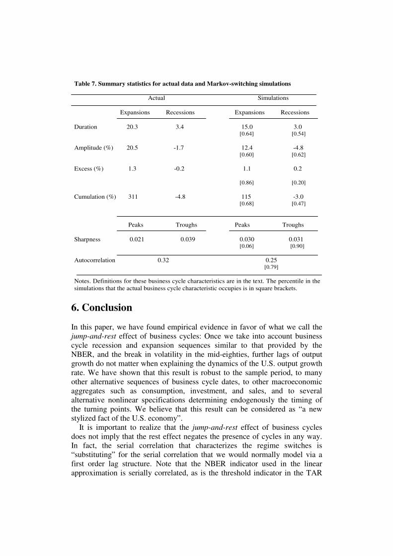
Table 7. Summary statistics for actual data and Markov-switching simulations

Actual Simulations

Expansions Recessions Expansions Recessions

Duration 20.3 3.4 15.0 3.0 [0.64] [0.54]

Amplitude (%) 20.5 -1.7 12.4 -4.8 [0.60] [0.62]

Excess (%) 1.3 -0.2 1.1 0.2

[0.86] [0.20]

Cumulation (%) 311 -4.8 115 -3.0 [0.68] [0.47]

Peaks Troughs Peaks Troughs

Sharpness 0.021 0.039 0.030 0.031

[0.06] [0.90]

Autocorrelation 0.32 0.25 [0.79]

Notes. Definitions for these business cycle characteristics are in the text. The percentile in the

simulations that the actual business cycle characteristic occupies is in square brackets.

6. Conclusion

In this paper, we have found empirical evidence in favor of what we call the

jump-and-rest effect of business cycles: Once we take into account business

cycle recession and expansion sequences similar to that provided by the

NBER, and the break in volatility in the mid-eighties, further lags of output

growth do not matter when explaining the dynamics of the U.S. output growth

rate. We have shown that this result is robust to the sample period, to many

other alternative sequences of business cycle dates, to other macroeconomic

aggregates such as consumption, investment, and sales, and to several

alternative nonlinear specifications determining endogenously the timing of

the turning points. We believe that this result can be considered as “a new

stylized fact of the U.S. economy”.

It is important to realize that the jump-and-rest effect of business cycles

does not imply that the rest effect negates the presence of cycles in any way.

In fact, the serial correlation that characterizes the regime switches is

“substituting” for the serial correlation that we would normally model via a

first order lag structure. Note that the NBER indicator used in the linear

approximation is serially correlated, as is the threshold indicator in the TAR

model, the transition function in the STAR model, and the state variable in the

Markov model. The switch variables are, then, accounting for cycles that were

previously accounted for by autocorrelation coefficients.

The consequences of this new fact for future empirical and theoretical

macroeconomic analysis are diverse and depend on the interest of the reader.

From an empirical point of view, these simple dynamics facilitate the

understanding and development of forecasts, they reduce to a minimum the

complexity of impulse response functions and dynamic multipliers, specially

those developed in nonlinear contexts, and they simplify the simulation and

calibration analysis by overcoming unsolved computational problems. From a

theoretical point of view, these findings provide empirical support to those

theoretical models that describe the data generating process of output growth

jumping between two equilibria of high and low growth. In addition, the jump-

and-rest dynamics add further for investigating the empirical reliability of

theoretical simulations. Finally, these dynamics may act as a guideline for

resuscitating theoretical models that were neglected when autoregressive

parameters were accepted as the source of the positive autocorrelation of

output growth.

References

[1] Andrews, D. (1993): “Test for parameter instability and structural change

with unknown change point,” Econometrica, 61, 821-856.

[2] Andrews, D., and W. Ploberger (1994): “Optimal tests when a nuisance

parameter is present only under the alternative,” Econometrica, 62, 1383-

1414.

[3] Azariadis, C., and B. Smith (1998): “Financial intermediation and regime

switching in business cycles,” American Economic Review, 85, 516-536.

[4] Camacho, M. (2004): “Vector smooth transition regression models for US

GDP and the composite index of leading indicators,” Journal of Forecasting,

23, 173-179.

[5] Campbell, J., and G. Mankiw (1987): “Are output fluctuations transitory?”

Quarterly Journal of Economics, 102, 857-880.

[6] Cochrane, J. (1988): “How big is the random walk in GNP?” Journal of

Political Economy, 96, 893-920.

[7] Cogley, T., and J. Nason (1995): “Output dynamics in real-business-cycle

models,” American Economic Review, 85, 492-511.

[8] Diebold, F., and R. Mariano (1995): “Comparing predictive accuracy,”

Journal of Business and Economic Statistics, 13, 253-263.

[9] Evans, G., S. Honkapohja, and P. Romer (1998): “Growth cycles,”

American Economic Review, 88, 495-515.

[10] Galbraith, J.W (2003): “Content horizons for univariate time-series

forecast,” International Journal of Forecasting, 19, 43-55.

[11] Hamilton, J. (1989): “A new approach to the economic analysis of

nonstationary time series and the business cycles,” Econometrica, 57, 357-

384.

[12] Hansen, B. (1999): “Testing for linearity,” Journal of Economic Surveys

13, 551-576.

[13] Harding, D., and A. Pagan (2002): “Dissecting the cycle: A

methodological investigation,” Journal of Monetary Economics, 40, 365-381.

[14] Harvey, D., S. Leybourne, and P. Newbold (1997): “Testing the equality

of prediction mean squared errors,” International Journal of Forecasting, 13,

281-291.

[15] Kim, Ch., and Ch. Nelson (1999): “Has the U.S. economy become more

stable? A Bayesian approach based on a Markov-switching model of the

business cycle,” The Review of Economics and Statistics, 81, 608-616.

[16] Kim, Ch., J. Morley, and J. Piger (2005): “Nonlinearity and the

permanent effects of recessions,” Journal of Applied Econometrics, 20, 291-

309.

[17] Morley, J., and J. Piger (2006): “The importance of nonlinearity in

reproducing business cycle features,” in C. Milas, P. Rothman, and D. van

Dijk, eds., Nonlinear Time Series Analysis of Business Cycles, Amsterdam:

Elsevier Science, 75-93.

[18] King, R., Ch. Plosser, J. Stock, and M. Watson (1991): “Stochastic trends

and economic fluctuations,” American Economic Review, 81, 819-840.

[19] McConnell, M., and G. Perez-Quiros (2000): “Output fluctuations in the

United States: What has changed since the early 80s?” American Economic

Review, 90, 1464-1476.

[20] McQueen, G., and S. Thorley (1993): “Asymmetric business cycle

turning points,” Journal of Monetary Economics, 31, 341-362.

[21] Nelson, Ch., and Ch. Plosser (1982): “Trends and random walks in

macroeconomic time series,” Journal of Monetary Economics, 10, 139-162.

[22] Potter, S. (1995): “A nonlinear approach to US GNP,” Journal of Applied

Econometrics, 10, 109-25.

[23] Teräsvirta, T. (1994): “Specification, estimation, and evaluation of

smooth transition autoregressive models,” Journal of the American Statistical

Association, 89, 208-218.

[24] Teräsvirta T. (1995): “Modelling nonlinearity in U.S. Gross national

product 1889-1987,” Empirical Economics, 20, 577-97.

[25] Tong, H. (1978): “On a threshold model,” in C.H. Chen, ed., Pattern

Recognition and Signal Processing, Amsterdam: Sijhoff and Noordhoff.

[26] Watson, M. (1986): “Univariate detrending methods with stochastic

trends,” Journal of Monetary Economics, 18, 49-75.

Jump-and-Rest Effect of U.S. Business Cycles

Documents

Transcript of Jump-and-Rest Effect of U.S. Business Cycles