Serial Number: NRB/WP/11

NRB Working Paper

Inflation Persistence in Nepal: A TAR Representation

T.P. Koirala, PhD Assistant Director, Nepal Rastra Bank, Research Department

NEPAL RASTRA BANK, RESEARCH DEPARTMENT

July 2012

© 2012 Nepal Rastra Bank Serial Number: NRB/WP/11

NRB Working Paper

Research Department

Inflation Persistence in Nepal: A TAR Representation

Prepared by T.P. Koirala*, PhD

Abstract This paper investigates inflation persistence under Threshold Autoregressive (TAR) model motivated by the fact that inflation in Nepal goes through different degrees of persistence based on various regime shifts. Using monthly time series of the Consumer Price Index (CPI) from 1998:01 to 2011:12, the presence of dynamic adjustment of inflation between high inflation and low inflation regimes defined by threshold inflation reveals non-linear behavior of inflation. A degree of low persistency is found in the high inflation regime. Low inflation persistence in high inflation regime signifies that inflation do not remain for a long period of time as a result of policy shocks pursued to trigger inflation down. Therefore, the policy shocks (such as monetary and fiscal policies) to bring inflation into low inflation regime cannot be ruled out in Nepal. Further, as the variance of the inflation shocks above the threshold is found greater than below the threshold, the policy shocks as well as shocks emanating from supply constraint and foreign inflation shocks are responsible in switching inflation from above the threshold to below the threshold.

Key Words: Inflation Persistence, Threshold Autoregressive (TAR) Model, Non-linear Model, Dynamic Adjustment, Regime shifts.

JEL Classification: C22, E31

∗ Assistant Director, Research Department, Nepal Rastra Bank, Central Office, Baluwatar, Kathmandu. E-mail:koiralat@nrb.org.np. This study is related to the paper presented in the International Conference on Economics and Finance organized by Nepal Rastra Bank (April 20-22, 2012) in Kathmandu, Nepal. The author has incorporated comments and suggestions raised during conference. Further the author is grateful to the anonymous referees for their valuable comments on this paper. The views expressed in this paper are personal and do not necessarily represent the official stance of Nepal Rastra Bank.

CONTENTS

Page

1. Introduction 1 2. Conceptual Framework 2 3. Methodology 3 4. Stylized Fact 4 5. Testing for Nonlinearity 5 6. Estimation of Threshold Inflation 6 7. Model Specification 7 8. Conclusion 8 References 9

1

1. INTRODUCTION

In contrast to the use of existing structural models identified previously in predicting inflation behavior in Nepal, the motivation of the paper is to make use of time series analysis to investigate inflation persistence of Nepal. Since inflation is partially anchored by its recent history in response to real activity and supply shocks, inflation is subject to persistent over time. Inflation tends to be persistent when the rate of change in the price level tends to remain constant in the absence of an economic force to move it from its current level. The behavior of persistency in inflation series is determined by the nature of variables explaining it where the latter variables may capture the effect of those errors arisen on account of exclusion and omitted variable bias in the identification of inflation model. In light of uncertainty in the specification of the structural model of inflation, modeling inflation based on its own historical values can also be theoretically justified. The physical analogy may provide motivating intuition for the study of inflation inertia in an environment of inflation persistence.

The effectiveness of monetary policy in controlling inflation in Nepal has been a prolonged debate among policymakers. The issue of the debate is that whether monetary policy is effective to anchor inflation. However, a common consensus is that monetary policy can, to some extent, control inflation but the relationship is not found so strong and robust (Nepal Rastra Bank, 2001) on account of the behavior of inflation to be integrated of policy as well as supply shocks in Nepal.

The phenomenon of inflation variation as a result of the changes in the prices of goods and services in the international market is one dominating factor in triggering inflation of Nepal. For example, fluctuation in the price of petroleum products in the international market is considered as an important foreign shock. Changes in world price will affect Nepalese price with a coefficient equal to unity (Pant, 1988). A study on inflation in Nepal conducted in Research Department, Nepal Rastra Bank (2007) also found that Indian inflation is one dominating factor determining inflation.

Though money supply is considered theoretically as a prominent factor determining inflation, the lack of consensus on significant lag-length as specified in the inflation dynamic is still ambiguous among the policymakers. There are varied lag responses of money supply on inflation (Sharma, 1992, Nepal Rastra Bank, 2001). Not only different monetary aggregates, but also a number of structural factors has been examined to show robust relationship of inflation. Khatiwada’s (1994) analysis found an improvement in explanatory power of the inflation model with the introduction of different structural variables. There is a positive relationship between inflation and inflation expectations in Nepal using model of adaptive expectation hypothesis (Koirala, 2008a). Though various structural models have been examined to gauge the inflation behavior in Nepal, the presence of volatility clustering of inflation in Nepal (Koirala, 2008b) has raised uncertainty in forecasting inflation in Nepal.

In view of the apparent difficulties in modeling inflation based on various structural models as mentioned above, modeling inflation in a setting of numerous shocks is a new area of research in Nepal. Controlling inflation in a surrounding of foreign and domestic shocks prevalent in the economy reduces the efficacy of monetary policy in particular and macroeconomic policies in general. As shocks being integrated or cumulated, there is tendency of sticky downward inflation to prevail. The persistent nature of inflation due to integrated or cumulative shocks rationalizes the use of inflation's own historical values in predicting future inflation rather than predicting the inflation depending on various structural factors determining inflation.

The majority of the empirical econometric modeling assumes that relationships between the variables are linear. The economic process assumed as linear can only provide approximate behavior of the actual time paths of economic variables (Enders, 2004). Based on the regularities observed in economic and financial data in different countries, non-linear specifications may be a more realistic representation of data generating processes. Policymakers

2

could make a serious error if they ignore the empirical evidence of the variables of interest pertaining to a sharper increase or decrease along the different phases of the business cycles.

The error correction model (ECM), a recent development in model specification, is a special case of non-varying coefficient of error correction term. The latter term so estimated cannot capture non-linear data generating process. The adjustment parameter represented by the coefficient of error correction term (ECT) in the studies on dynamic mechanism of inflation determination in Nepal by Pandey (2005), Nepal Rastra Bank (2007), (Bishnoi and Koirala (2008) may not represent true adjustment process if the adjustment parameters estimated so in those studies are not considered invariant over time. Standard cointegration models assume linearity and symmetric adjustment although actual data generating process may possess asymmetric adjustment (Engle and Granger, 1987). The threshold autoregressive (TAR) model is one variant of dynamic model that incorporates the option of asymmetric adjustment in different regimes of data generating process. When adjustment is symmetric in the error-correction term, TAR reduces to the error correction model (Balke and Fomby, 1997; Enders and Granger, 1998; Enders and Siklos, 2000).

The study of inflation persistence under the possibility of asymmetric adjustment in different regimes of the economy specified by threshold inflation is new area of research in Nepal. In view of this, the specific objective of this paper is to identify degrees of inflation persistence in different regimes of the economy based on threshold inflation and to evaluate factors causing the regimes to shift. Further, a study of inflation persistence under nonlinear framework, as this study focuses on, offers some guidelines to policy makers to identify level of inflation in different regimes and hence to adopt controlling measures in varying degrees of inflation persistence depending on different regimes. Following the threshold regressive model for the monthly data frequency of inflation from 1998:01 to 2011:12, some interesting conclusions in this paper have been drawn that the big shocks above the threshold inflation are responsible for switching inflation above the threshold to below the threshold. Therefore, the policy shock to maintain inflation into low inflation regime does matter. In other words, the effectiveness of monetary and fiscal policy in order to bring and then maintain the inflation below the threshold level cannot be ruled out.

The rest of the paper is organized as follows. Section 2 discusses the use of non-linear models to capture asymmetries behavior of the variables of interest under the heading ‘Conceptual Framework’. The methodology of the paper is presented in section 3 followed by stylized fact of the inflation behavior of Nepal in section 4. The testing for non-linearity of inflation sequence, estimated threshold inflation and model specification in the analysis are presented subsequently in sections 5, 6 and 7. The conclusion of this study is presented in section 8.

2. CONCEPTUAL FRAMEWORK Nonlinear models have been widely applied in recent years to capture asymmetries and jump phenomena in the behavior of economic and financial time series. In finance, for instance, stock returns tend to be more correlated when there is low volatility than when volatility is high. Hamilton (1988) introduced a regime-switching model of interest rates in which the public learn about the underlying state of the economy and to use this knowledge when pricing bonds. A similar behavior has been observed in exchange rate mechanisms where the exchange rate is constrained to lie within a pre-defined target regime (Franses and Dijk, 2000). In agricultural marketing, there exist asymmetries in price adjustments at various levels of the food marketing system (Hector O. Zapata and Wayne M. Gauthier, 2003). A similar argument has been put forward in the literature on spatial market integration where transfer costs cause threshold effects and that leads to equilibrium in spatially separated markets (Kharel and Koirala, 2011).

Among the non-linear models, one particular model that is regularly appeared in the economics literature is the threshold autoregressive (TAR). The TAR model can have limit cycles and thus be used to model periodic time series or to produce asymmetries and jump phenomena that

3

cannot be captured by the linear time series model like autoregressive (AR) model. The TAR model introduced by Tong and Lim (1980) and extensive discussion in Tong (1990) has received tremendous currency in the field of empirical analysis on various economic phenomenons. Regime-switching models (RSM) introduced by Priestley (1980) is one variant of TAR model which is used to capture asymmetric and jump phenomenon in the studies of Granger and Terasvirta (1993). Enders and Granger (1998) extended the simple linear model to a two-state regime switching threshold autoregressive model and found two roots to capture the adjustment process in this model, one governing the economic downturns and other economic upturns (Balke and Fomby, 1997). The smooth transition threshold autoregressive (STAR) model of Chan and Tong (1986) and Teräsvirta (1994) is the extended version of the TAR model, and it is used to reflect the idea that variables of interest possess different dynamics when the values of the variables are unusually high or low.

The TAR model for the analysis of inflation dynamic can be derived by simple extension of AR(1) representation of the model as:

ttt u++= −11πβαπ . (1)

Where, tπ and 1−tπ are current and one period lag inflation rates respectively. The 1β shows degree of persistence from last period to current period inflation and stability condition requires

11 <β or root of the equation (1) lies inside the unit circle. The tu satisfies iid condition. Defining π as a long-run inflation )1/( 1βα − and writing the adjustment process as:

ttt v+−+= − )( 11 ππβππ (2)

If ππ =t , the system is said to be in long-run equilibrium. The parameter 1β implies the degree of persistence, that is, the percentage of the deviation in one period lag inflation to the long-run value. It is assumed that the spread of current inflation to its long-run value displays a non-linear or asymmetric adjustment process. The degree of adjustment when the spread is high relative to its long-run value )0( 1 >−− ππ t may be different from the adjustment when the spread is low )0( 1 <−− ππ t . The separation of models representing different degrees of persistence based on threshold inflation (π ) can be modeled as:

=tπ )( 11 ππβπ −+ −t when ππ >−1t (3)

=tπ )( 12 ππβπ −+ −t when ππ ≤−1t (4)

As long as 21 ββ ≠ , the degrees of persistence in equation (3) and (4) are different based on greater or smaller values of 1−tπ from long-run value π .

3. METHODOLOGY The TAR model is the simple generalization of an AR model that allows for the data analysis depending on its past values of corresponding to different regimes. The dynamic adjustment equation for inflation depends on whether the economy is in an inflationary state (or regime) or in a deflationary. When the economy changes from an inflationary regime to a deflationary regime, the dynamic adjustment of the variable of inflation is likely to change. Therefore, the TAR model allows the behavior of { }tπ to depend on the state of the system. The notion underlying the TAR model is piecewise linearization of non-linear models over the state space by the introduction of the thresholds. TAR models have also been used successfully to explore asymmetries in macroeconomic variables over the course of the business cycle. The basic concern in formulating TAR model is that whether the apparent persistence in time series

4

variables provides evidence of asymmetries that standard Gaussian linear (fixed) parameter models cannot accommodate (Enders 2004).

By assuming threshold inflation equals zero ( 0=π ) and inequality holds true for 1β and 2β ( 21 ββ ≠ ) as in equations (3) and (4), two separate AR(1) processes can be deduced for the estimation in this paper as depicted in equations (5) and (6). Those processes possess distinct regimes followed by discontinuous phase diagram (kinked line) representing different degrees of persistence in each regime. By assuming absence of drift term in respective equations, they appear as:

ttt u111 += −πβπ if τπ >−1t (5)

ttt u212 += −πβπ if τπ ≤−1t (6)

The compact form of equation (5) and (6) by creating indicator function ( tI ) to form the variables ittI −π and ittI −− π)1( as:

t

r

iitit

p

iititt II επββπββπ +

+−+

+= ∑∑

=−

=−

1220

1110 )1( (7)

When τπ >−1t , 1=tI and 0)1( =− tI , so that equation (7) is equivalent to

ttptt u11111110 ... ++++= −− πβπββπ . When τπ ≤−1t , 0=tI and 1)1( =− tI , so that

equation (7) is equivalent to trtrrtt u222120 ... ++++= −− πβπββπ .

In case the value of τ is unknown, it should be estimated through the data so that it is considered super-consistent estimate (Enders, 2004). If the inflation data cross each time the threshold (τ ), a meaningful value of τ is obtained. Therefore, τ should lie within the maximum and minimum value of data sequence. The highest and lowest fifteen percent of the data are excluded from the search process of threshold value (Chan, 1993).

Monthly time series of the Consumer Price Index (CPI) from 1998:01 to 2011:12 has been utilized in this study. The period of the analysis has been selected based on the calm period before the period of big economic shocks as a result of political turmoil initiated in the year 2001. Such an initial period as selected here is considered as benchmark to analyze the magnitude and propensity of business cycle created by economic shocks. Monthly inflation rates have been derived based on percentage changes of CPI to this month to the corresponding month of the last year. The sequence of inflation rates { }tπ so derived is assumed to rule out seasonality problem. The threshold autoregressive (TAR) model as presented in equation (7) is utilized for the analysis of various regimes of inflation. The observations lying above and below the τ are obtained using indicator function. Maximum and minimum 15 percent of the inflation sequence { }tπ is trimmed out to estimate threshold value (τ ) in this study. A grid search process is adopted to estimate threshold value (τ ) and the value that minimizes the sum of squares residual is considered unbiased and consistent threshold value (τ ).

4. STYLIZED FACT The phases and amplitudes of inflation business cycles is an important for the formulation of macroeconomic polices in general and monetary policy in particular. As monetary policy aims to keep inflation within the target band so as to ensure economic stability and sustainable growth, it is inevitable to know the likely inflation regimes in advance for adopting appropriate policy measures. The mean of 185 monthly inflation rates from the January 1998 to December 1011 is 7.20 percent. Inflation of Nepal during the study period shows the standard deviation of 4.12 percent showing high volatility. The inflation rates fluctuate within the highest rate of 18

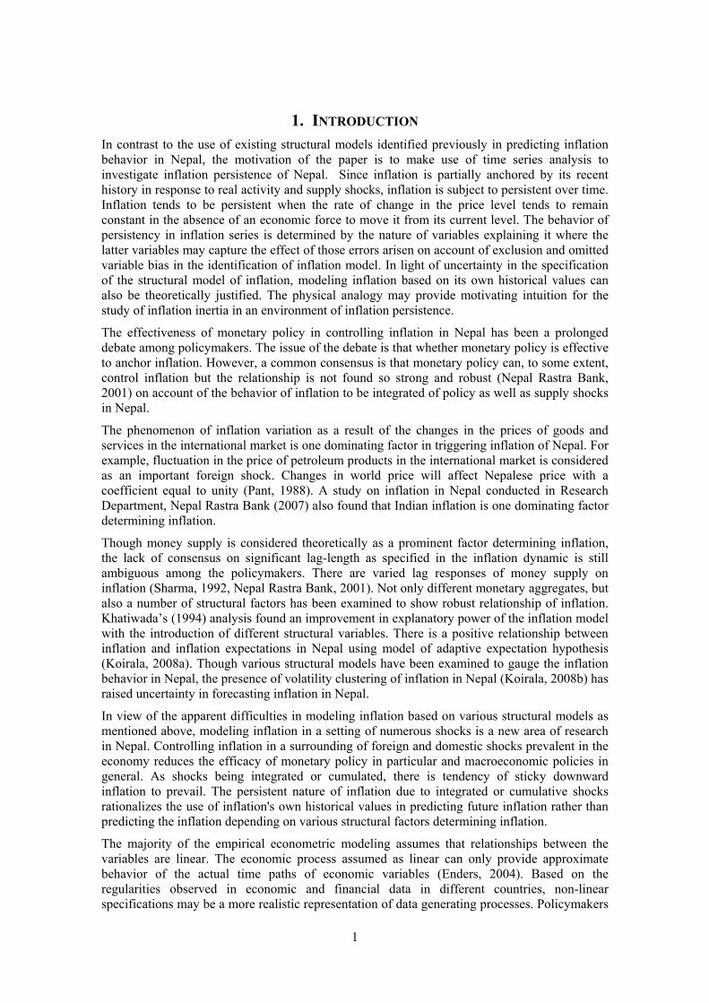
5

percent in November 1998 to negative of 0.51 percent in July 2000. The trend and cyclical pattern of inflation rates are presented in Figure 1. The rate of decline alongside the initial period of the cycle is higher than that of the rates of increase alongside the upward trend. The true non-linear data generating process as such depicted in the figure may not be captured by linear model. In modeling nonlinear behavior of inflation in Nepal, it is allowed for the existence of different states of the regimes corresponding to different dynamics in those regimes. Prior to the identification of states of regime, the presence of non-linearity in the data generating process should be checked as a prerequisite for the TAR model specification.

5. TESTING FOR NONLINEARITY In testing the presence of non-linearity in the data generating process of inflation, we follow two steps process. Firstly, the linear portion of the AR(p) model is estimated to determine autoregressive of order p. Secondly, we identify the non-linearity in the inflation sequence { }tπ by checking the statistically significance AR(p) process of residual sequence { }tε generated based on the best fit AR(p) model. The criterion for the selection of lag length or order of p value in AR(p) specification is that the lag length which minimizes the AIC and SC values.

Table 1: Specification of best fit AR(p) process of inflation { }tπ

Specification Constant Lag 1 Lag 2 Lag 3 Lag 4 AIC value

SC Value

1 0.34 (0.19)

1.11 (0.08)

-0.19 (0.12)

0.05 (0.12)

-0.03 (0.08)

3.21 3.31

2 0.33 (0.19)

1.11 (0.08)

-0.18 (0.12)

0.02 (0.08)

-

3.20 3.27

3 0.34 (0.18)

1.11 (0.08)

-0.16 (0.08)

- 3.18 3.23

4 0.30 (0.18)

0.96 (0.02)

- - - 3.19 3.24

5 7.21 (0.31)

- - - - 5.68 5.69

Note: Figures in parenthesis are standard error of respective coefficients.

Following AIC and SC, the best fit AR(p) process of inflation happens to be specification no. 3. Therefore, inflation during the study period, possesses AR(2) process based on grid search process among the five specification of AR(p) presented in Table 1. The best fit AR(p) model of inflation can be represented in equation form as follows:

tttt u+−+= −− 21 16.011.134.0 πππ (8)

t: (1.84) (14.29) (-2.04) 2R = 0.91 DW=1.99

The residual sequence { }tε so derived based on equation (8) has been used to test the non-linearity of inflation sequence{ }tπ . Under the null hypothesis of all the coefficients of AR(p)

6

for the squared residuals sequence { }2tε are simultaneous equal to zero indicates non existence

of linearity in the { }tπ .

Table 2: Specification of AR(p) process on Squared Residual Error { }2tε

Specification Constant Lag 1 Lag 2 Lag 3 Lag 4 AIC SC 1 1.29

(0.29) -0.06 (0.08)

-0.21 (0.08)

-0.06 (0.8)

-0.05 (0.08)

4.79 4.88

2 1.23 (0.27)

-0.06 (0.07)

0.20 (0.08)

-0.06 (0.09)

-

4.77 4.85

3 1.19 (0.26)

-0.08 (0.07)

0.21 (0.08)

- 4.76 4.82

4 1.49 (0.23)

-0.09 (0.07)

- - - 4.79 4.83

Note: Figures in parenthesis are standard error of respective coefficients.

Simultaneously statistically non-significance of AR(2) process for { }2tε in the specification no.

3 of Table 2 (based on minimum value of AIC and SC statistics) clearly indicates that inflation series under review follows non-linear pattern.

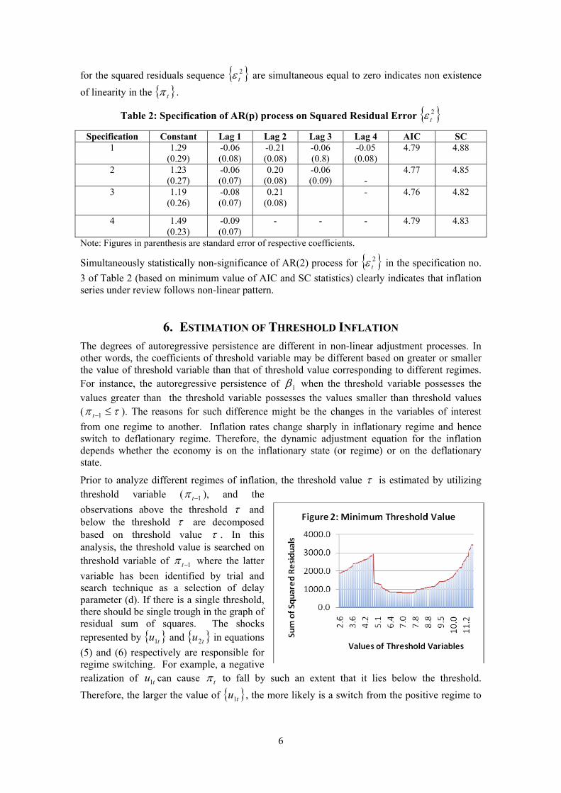
6. ESTIMATION OF THRESHOLD INFLATION The degrees of autoregressive persistence are different in non-linear adjustment processes. In other words, the coefficients of threshold variable may be different based on greater or smaller the value of threshold variable than that of threshold value corresponding to different regimes. For instance, the autoregressive persistence of 1β when the threshold variable possesses the values greater than the threshold variable possesses the values smaller than threshold values ( τπ ≤−1t ). The reasons for such difference might be the changes in the variables of interest from one regime to another. Inflation rates change sharply in inflationary regime and hence switch to deflationary regime. Therefore, the dynamic adjustment equation for the inflation depends whether the economy is on the inflationary state (or regime) or on the deflationary state.

Prior to analyze different regimes of inflation, the threshold value τ is estimated by utilizing threshold variable ( 1−tπ ), and the observations above the threshold τ and below the threshold τ are decomposed based on threshold value τ . In this analysis, the threshold value is searched on threshold variable of 1−tπ where the latter variable has been identified by trial and search technique as a selection of delay parameter (d). If there is a single threshold, there should be single trough in the graph of residual sum of squares. The shocks represented by { }tu1 and { }tu2 in equations (5) and (6) respectively are responsible for regime switching. For example, a negative realization of tu1 can cause tπ to fall by such an extent that it lies below the threshold. Therefore, the larger the value of { }tu1 , the more likely is a switch from the positive regime to

7

the negative regime. If τπ >−1t , the subsequent values of the sequence tends to decay toward threshold value at the rate of 1β .

So far as the estimation of threshold is concerned, we take deviations of the series from each of the values in the series as threshold value. After squaring and then summing up each of the deviation series yield value of threshold τ based on the minimization of the sum of squared residual of mean reversion model. Out of 167 observations used in this analysis, 15 percent observations in each side of shorted sequence { }1−tπ have been eliminated in the grid search process by considering those observations lying outside the threshold band. The graphical depiction of 118 residual sum of squares based on observations contained in the threshold band is presented in Figure 3. Corresponding the value of 59th observation, the inflation rate of 7.14 percent is found to be threshold value under the smallest value of residual sum of squares criteria.

7. MODEL SPECIFICATION Two inflation sequences{ }tπ , one belongs to above the threshold and other below the threshold, possess distinct autoregressive process. Therefore, there are two regimes specified in this analysis. Although inflation sequences { }tπ are linear in each regime, the possibility of regime switching means that the entire { }tπ sequence is non-linear. The two separate autoregressive processes based on estimated threshold value in the present study are presented in the equations (9) and (10) respectively as follows:

1178.083.1 ttt u++= −ππ 1β if 14.71 >−tπ (9)

t : (1.61) (6.57) 2R = 0.42 DW=1.71 Obs: 58

210.111.0 ttt u++= −ππ 2β if 14.71 ≤−tπ (10)

t : (0.23) (11.05) 2R = 0.68 DW=1.66 Obs: 59

Provided the threshold value, distinct autoregressive coefficients as found here depict different data generating processes in two states of the economy. For example, the coefficient of inflation persistence when 14.71 >−tπ is 0.78 (in equation 9) depicts one inflation behavior whereas coefficient 1.01 (in equation 10) shows different inflation behavior. Inflation is found more persistent in the low inflation regime than that of high inflation regime. Different degrees of persistence are characterized by the visual inspection of the time paths (as shown in figure 4 and 5) based on simulated random walk with a series of 100 normally distributed random variates drawn from a theoretical distribution with a mean of zero and a variance equal to unity.

2178.0 ttt u+= −ππ 110.1 ttt u+= −ππ

8

The series mender without any tendency to revert to a long-run value when the autoregressive coefficient is unity (figure 4) whereas the mean reversion is more pronounced in case the coefficient is less than unity (i.e. 0.78) (figure 5).

Further, the magnitude of the shocks above the threshold, as represented by estimated variance of { }1tu , is found to be quite large { } 19.11 =tu compared to that of the shocks below the threshold{ } 85.02 =tu , implies that big shocks are responsible for the regime switching to occur. The estimated coefficients of inflation persistence and variances of shocks so obtained in this analysis draw some interesting conclusion as:

• There is the tendency of high inflation to decay readily toward threshold inflation in Nepal. The policy shocks (monetary and fiscal policies) that are used to bring inflation towards the threshold level or even in maintaining inflation within the low inflation regime cannot be ruled out.

• The policymakers may respond differently to changes in economic variables in a high inflationary environment than in a low inflationary environment. The monetary authority may contribute growth objectives of the government of Nepal under the low inflationary regime defined by the threshold value in this paper.

• The big exogenous shocks of the inflation originating either from lack of smooth supply of goods in the domestic market or from slow adjustment of prices of goods and services in the domestic market compared to that of foreign market may be responsible for regime switching to occur.

8. CONCLUSION This paper examines inflation persistence in Nepal using threshold autoregressive model introduced by Tong and Lim (1980) using the monthly inflation data from 1998:01 to 2011:12. Assuming threshold inflation as the benchmark of regime switching to occur, inflation is found less persistent in the high inflation regime than that of low inflation regime. As the high inflation rates are readily decay towards the threshold inflation rate, as found in this study, implies that the exogenous and policy shocks that are responsible for high inflation are no longer persist above the threshold value. Low inflation persistence in high inflation regime implies that inflation remain in the high inflation regime for a very short period of time as a result of contractionary policies being pursued. Further, the policy shocks that are used in bringing inflation into the low inflation regime seem effective. Since the magnitude of the shocks above the threshold tends to be quite large compared to the shocks below the threshold, the big shocks (i.e. policy and exogenous shocks) above the threshold are responsible for switching the regimes from above the threshold to below the threshold.

9

REFERENCES

Balke, N. S. and T. B. Fomby (1997). “Threshold Cointegration,” International Economic Review, 38: 627-45.

Bishnoi, T.R. and T.P. Koirala (2006). “Stability and Robustness of Inflation Model Of Nepal: An Econometric Analysis,” Journal of Quantitative Economics, no.2, Journal of the Indian Econometric Society, Mumbai, India.

Chan, K.S. (1993). “Consistency and Limiting Distribution of the Least Squares Estimator of a Threshold Autoregressive Model,” The Annals of Statistics 21: 520-33.

Chan, K.S. and H. Tong (1986). “On Estimating Thresholds in Autoregressive Models, Journal of Time Series Analysis, 7: 179-190.

Enders, W. (2004), “Applied Econometric Time Series,” John Wiley & Sons (ASIA) Pte Ltd., Singapore.

----- and C. W. J. Granger (1998). “Unit-Root Tests and Asymmetric Adjustment with an Example Using the Term Structure of Interest Rates,” Journal of Business and Economic Statistics, 16:304-11.

----- and P. L. Siklos (2001). “Cointegration and Threshold Adjustment,” American Statistical Association Journal of Business and Economic Statistics, 19:166-76.

Engle, R.F. and C.W.J. Granger (1987). “A Cointegration and Error Correction: Representation, Estimation and Testing,” Econometrica, 55: 251-76.

Franses, P. H. and D. V. Dijk (2000). “Non-linear Time Series Models in Empirical Economics”, New York, Cambridge University Press.

Granger, C. W. J. and T. Terasvirta (1993). “Modeling Nonlinear Economic Relationships,” Oxford University Press, Oxford, U.K.

Hamilton, J.D. (1988). “Rational Expectations Econometric Analysis of Changes in Regime: An Investigation of the Term Structure of Interest Rates,” Journal of Economic Dynamics and Control, 12: 385-423.

Hector, O. Z. and W. M. Gauthier (2003). “Threshold Models in Theory and Practice,” Department of Agribusiness and Agri-Economics, Louisiana State University, Baton Rouge, Louisiana, USA.

Kharel, R.S. and T.P. Koirala (2011). “Spatial Price Integration in Nepal”, Economic Review (Occasional Paper), Nepal Rastra Bank, Kathmandu, Nepal.

Khatiwada, Y.R. (1994). “Some Aspects of Monetary Policy in Nepal”, South Asian Publishers, New Delhi, India.

Koirala, T.P. (2008a). “Inflation Expectations in Nepal”, Economic Review, Occasional Paper 20, Nepal Rastra Bank, Kathmandu, Nepal.

----- (2008b). “Volatility Clustering of Inflation in Nepal: An ARCH Specification”, The Economic Journal of Nepal, 31, no.1, Department of Economics, The Tribhuvan University, Kathmandu, Nepal.

Nepal Rastra Bank (2001). “Money and Price Relationship in Nepal: A Revisit”, Economic Reviews, Occasional Paper, no.13.

Nepal Rastra Bank (2007), “Inflation in Nepal”, Research Department, Kathmandu, Nepal.

Pant, R.D. (1988). “Sources of Inflation in Asia: Theory and Evidences”, Nirala Publications, Jaipur, New Delhi, India.

10

Pandey, R.P. (2005). “Inflation”, Nepal Rastra Bank in Fifty Years, Nepal Rastra Bank, Kathmandu, Nepal.

Priestley, M. B. (1980). “State-Dependent Models: A General Approach to Non-Linear Time Series Analysis,” Journal of Time Series Analysis, 1: 47-71.

Priestley, M. B. (1988). “Non-Linear and Non-Stationary Time Series Analysis”, New York: Academic Press.

Sharma, V.R. (1992). “Inflation in Nepal”, The Economic Journal of Nepal, 15 no.4, Tribhuvan University, Kathmandu, Nepal.

Teräsvirta, T. (1994). “Specification, Estimation, and Evaluation of Smooth Transition Autoregressive Models,” Journal of the American Statistical Association 89, 208-218.

Tong, H. (1978). “On a Threshold Model” in C. H. Chen, ed., "Pattern Recognition and Signal Processing" Sijhoff and Noordoff, Amsterdam, 100-141.

----- (1980). “Catastrophe Theory and Threshold Autoregressive Modeling”, Technical Report no. 125, Department of Mathematics, UMIST.

------ (1990). “Non-Linear Time Series: A Dynamic System Approach,” Oxford: Oxford University Press.

------ and K. S. Lim (1980). “Threshold Autoregression, Limit Cycles, and Cyclical Data” J. R. Statist. Soc., Ser. B, 42, 245-292.