J.turbomachinery.2007.Vol.129.N1

Editor, DAVID C. WISLER „2008…Assistant to the Editor: ELIZABETH WISLER

Associate EditorsGas Turbine �Review Chair�

K. MILLSAPS, JR. „2007…Aeromechanics

M. MONTGOMERY „2008…A. SINHA „2008…

Boundary Layers and TurbulenceG. WALKER „2008…

Computational Fluid DynamicsJ. ADAMCZYK „2008…

M. CASEY „2008…Experimental Methods

W.-F. NG „2008…Heat Transfer

J.-C. HAN „2008…K. A. THOLE „2007…

Radial TurbomachineryR. VAN DEN BRAEMBUSSCHE „2008…

Turbomachinery AeroS. GALLIMORE „2008…

D. PRASAD „2008…A. R. WADIA „2009…

PUBLICATIONS COMMITTEEChair, BAHRAM RAVANI

OFFICERS OF THE ASMEPresident, TERRY E. SHOUP

Executive Director, VIRGIL R. CARTERTreasurer, T. PESTORIUS

PUBLISHING STAFFManaging Director, Publishing

PHILIP DI VIETROManager, JournalsCOLIN MCATEER

Production CoordinatorJUDITH SIERANT

Production AssistantMARISOL ANDINO

Transactions of the ASME, Journal of Turbomachinery�ISSN 0889-504X� is published quarterly �Jan., Apr., July, Oct.� by

The American Society of Mechanical Engineers, Three Park Avenue,New York, NY 10016. Periodicals postage paid at

New York, NY and additional mailing offices.POSTMASTER: Send address changes to Transactions

of the ASME, Journal of Turbomachinery, c/o THEAMERICAN SOCIETY OF MECHANICAL ENGINEERS,

22 Law Drive, Box 2300, Fairfield, NJ 07007-2300.CHANGES OF ADDRESS must be received at Society

headquarters seven weeks before they are to be effective.Please send old label and new address.

STATEMENT from By-Laws. The Society shall not beresponsible for statements or opinions advanced in papers

or ... printed in its publications �B7.1, Par. 3�.COPYRIGHT © 2007 by the American Society of

Mechanical Engineers. For authorization to photocopy materialfor internal or personal use under those circumstances not falling

within the fair use provisions of the Copyright Act, contact theCopyright Clearance Center �CCC�, 222 Rosewood Drive,

Danvers, MA 01923, tel: 978-750-8400, www.copyright.com.Request for special permission or bulk copying should be

addressed to Reprints/Permission Department.Canadian Goods & Services Tax Registration #126148048

TECHNICAL PAPERS1 Predicting Transition in Turbomachinery—Part I: A Review and New

Model DevelopmentT. J. Praisner and J. P. Clark

14 Predicting Transition in Turbomachinery—Part II: Model Validation andBenchmarking

T. J. Praisner, E. A. Grover, M. J. Rice, and J. P. Clark

23 Experimental and Computational Comparisons of Fan-Shaped FilmCooling on a Turbine Vane Surface

W. Colban, K. A. Thole, and M. Haendler

32 The Effect of Hot-Streaks on HP Vane Surface and Endwall Heat Transfer:An Experimental and Numerical Study

T. Povey, K. S. Chana, T. V. Jones, and J. Hurrion

44 Experimental Evaluation of Active Flow Control Mixed-Flow Turbine forAutomotive Turbocharger Application

Apostolos Pesiridis and Ricardo F. Martinez-Botas

53 A Direct Performance Comparison of Vaned and Vaneless Stators forRadial Turbines

S. W. T. Spence, R. S. E. Rosborough, D. Artt, and G. McCullough

62 Aerodynamic Design and Testing of Three Low Solidity Steam TurbineNozzle Cascades

Bo Song, Wing F. Ng, Joseph A. Cotroneo, Douglas C. Hofer, andGunnar Siden

72 Aeroelastic Stability of Welded-in-Pair Low Pressure Turbine RotorBlades: A Comparative Study Using Linear Methods

Roque Corral, Juan Manuel Gallardo, and Carlos Vasco

84 The Effect of Work Processes on the Casing Heat Transfer of a TransonicTurbine

Steven J. Thorpe, Robert J. Miller, Shin Yoshino,Roger W. Ainsworth, and Neil W. Harvey

92 Effect of Reynolds Number and Periodic Unsteady Wake Flow Conditionon Boundary Layer Development, Separation, and Intermittency BehaviorAlong the Suction Surface of a Low Pressure Turbine Blade

M. T. Schobeiri, B. Öztürk, and David E. Ashpis

108 Improving Aerodynamic Matching of Axial Compressor Blading Using aThree-Dimensional Multistage Inverse Design Method

M. P. C. van Rooij, T. Q. Dang, and L. M. Larosiliere

119 Axial Compressor Deterioration Caused by Saltwater IngestionElisabet Syverud, Olaf Brekke, and Lars E. Bakken

127 Experimental Investigation of the Effects of a Moving Shock Wave onCompressor Stator Flow

Matthew D. Langford, Andrew Breeze-Stringfellow,Stephen A. Guillot, William Solomon, Wing F. Ng, andJordi Estevadeordal

136 Online Water Wash Tests of GE J85-13Elisabet Syverud and Lars E. Bakken

143 Advanced Modeling of Underplatform Friction Dampers for Analysis ofBladed Disk Vibration

E. P. Petrov and D. J. Ewins

Journal ofTurbomachineryPublished Quarterly by ASME

VOLUME 129 • NUMBER 1 • JANUARY 2007

„Contents continued on inside back cover…

Downloaded 31 May 2010 to 128.113.26.88. Redistribution subject to ASME license or copyright; see http://www.asme.org/terms/Terms_Use.cfm

http://scitation.aip.org/getpdf/servlet/GetPDFServlet?filetype=pdf&id=JOTUEI000129000001000001000001&idtype=cvips
















































151 Effect of Tip and Pressure Side Coolant Injection on Heat Transfer Distributions for a Plane and Recessed TipHasan Nasir, Srinath V. Ekkad, and Ronald S. Bunker

164 Making Use of Labyrinth Interaction FlowA. Pfau, A. I. Kalfas, and R. S. Abhari

175 On a Novel Annular Sector Cascade TechniqueT. Povey, T. V. Jones, and M. L. G. Oldfield

184 Preliminary Fan Design for a Silent AircraftDaniel Crichton, Liping Xu, and Cesare A. Hall

The ASME Journal of Turbomachinery is abstracted and indexedin the following:Aluminum Industry Abstracts, Aquatic Science and Fisheries Abstracts, CeramicsAbstracts, Chemical Abstracts, Civil Engineering Abstracts, Compendex (The electronicequivalent of Engineering Index), Corrosion Abstracts, Current Contents, EiEncompassLit, Electronics & Communications Abstracts, Energy Information Abstracts,Engineered Materials Abstracts, Engineering Index, Environmental Science andPollution Management, Excerpta Medica, Fluidex, Fuel and Energy Abstracts, INSPEC,Index to Scientific Reviews, Materials Science Citation Index, Mechanical &Transportation Engineering Abstracts, Mechanical Engineering Abstracts, METADEX(The electronic equivalent of Metals Abstracts and Alloys Index), Metals Abstracts,Oceanic Abstracts, Pollution Abstracts, Referativnyi Zhurnal, Shock & Vibration Digest,Steels Alert

„Contents continued…

Journal of Turbomachinery JANUARY 2007Volume 129, Number 1










T. J. PraisnerTurbine Aerodynamics,

United Technologies Pratt & Whitney,400 Main St., M/S 169-29,

East Hartford, CT 06108

J. P. ClarkTurbine Branch,

Turbine Engine Division,Propulsion Directorate,

Air Force Research Laboratory,Building 18, Room 136D,

1950 5th St.,WPAFB, OH 45433

e-mail: [email protected]

Predicting Transition inTurbomachinery—Part I:A Review and New ModelDevelopmentHere we report on an effort to include an empirically based transition modeling capa-bility in a Reynolds Averaged Navier-Stokes solver. Well known empirical models for bothattached- and separated-flow transition were tested against cascade data and foundunsuitable for use in turbomachinery design. Consequently, a program was launched todevelop models with sufficient accuracy for use in design. As a first step, accurate pre-diction of free stream turbulence development was identified as a prerequisite for accu-rate modeling. Additionally, a demonstrated capability to capture the effects of freestream turbulence on pre-transitional boundary layers became an impetus for the work. Acomputational fluid dynamics (CFD)-supplemented database of 104 experimental cas-cade cases was constructed to explore the development of new correlations. Dimensionalanalyses were performed to guide the work, and appropriate non-dimensional parameterswere then extracted from CFD predictions of the laminar boundary layers existing on theairfoil surfaces prior to either transition onset or incipient separation. For attached-flowtransition, onset was found to occur at a critical ratio of the boundary-layer diffusiontime to a time scale associated with the energy-bearing turbulent eddies. In the case ofseparated-flow transition, it was found that the length of a separation bubble prior toturbulent reattachment was a simple function of the local momentum thickness at sepa-ration and the overall surface length traversed by a fluid element prior to separation.Both the attached- and separated-flow transition models were implemented into the de-sign system as point-like trips. �DOI: 10.1115/1.2366513�

IntroductionIn axial-flow turbomachinery, the design trend is toward in-

creasing airfoil loading in an effort to reduce weight and cost offuture systems. Transition prediction is critical for accurate losspredictions of high lift airfoils, and the full multi-moded �Mayle�1�� nature of the transition process must be considered. Lakshmi-narayana �2�, Simoneau and Simon �3�, Simon and Ashpis �4�,Dunn �5�, and Yaras �6� all provide detailed reviews of the state ofthe art in predictive techniques for turbomachinery, and they pointto the need for improved models for transition.

Elevated levels of free stream turbulence �Tu�1.0% � have asignificant effect on pre-transitional, or “quasi-laminar �QL�”boundary layers. Further, it is the authors’ opinion that the qualityof the laminar boundary layer at transition onset must be predictedaccurately before transition modeling can be used most effec-tively. Therefore, it is important to capture accurately the field-wise development of free stream turbulence quantities. To thatend, the ability of the k-� turbulence model of Wilcox �7� topredict the development of Tu was validated against the experi-mental data of Ames �8�. Additionally, an accurate technique formodeling the effects of Tu on laminar boundary layers within theframework of the k-� model was developed.

In testing against cascade data it was found that open-literaturemodels for attached and separated-flow transition were not suffi-ciently accurate for implementation in a design system. Conse-quently, an effort was launched to develop new correlations for

attached- and separated-flow transition. A dimensional analysiswas performed considering all transition-relevant quantities avail-able within the framework of a Reynolds Averaged Navier-Stokes�RANS� simulation performed with a two-equation turbulencemodel. A database of the resulting dimensionless groups was con-structed from open-literature and Pratt & Whitney in-house cas-cade data. The cascade data were supplemented with quantitiesbased on the aforementioned modeling techniques for free streamturbulence development and its effects on laminar boundary lay-ers. An investigation of the resulting database enabled the devel-opment of new models for attached- and separated-flow transition.The details of this process are documented below.

A computational-methods section will be presented first withdiscussions on boundary conditions, free-stream-disturbancepropagation and quasi-laminar boundary layers. Then, sectionsconcerning attached- and separated-flow transition are presented,where reviews of the state-of-the-art and current model develop-ment details are discussed. Validation and benchmarking of thenew models is presented in Part II of this paper.

Computational MethodsSteady-state and time-resolved turbine flow fields were pre-

dicted using the three-dimensional �3D�, Reynolds AveragedNavier-Stokes �RANS� code described both by Ni �9� and Daviset al. �10�. Numerical closure for turbulent flow is obtained via thek-� model of Wilcox �7�. An O-H grid topology was employed forall simulations, and approximately 600,000 grid points per pas-sage were used for three-dimensional simulations executed forthis study �without tip clearance�. The viscous grid provides near-surface values of y+ less than 1 over no-slip boundaries and givesapproximately 7 grid points per momentum thickness in airfoiland end wall boundary layers. These grid densities and spacingsprovide essentially grid-independent solutions for capturing ther-

Contributed by the International Gas Turbine Institute �IGTI� of ASME for pub-lication in the JOURNAL OF TURBOMACHINERY. Manuscript received October 1, 2003;final manuscript received March 1, 2004. IGTI Review Chair: A. J. Strazisar. Paperpresented at the International Gas Turbine and Aeroengine Congress and ExhibitionVienna, Austria, June 13–17, 2004, Paper No. 2004-GT-54108.

Journal of Turbomachinery JANUARY 2007, Vol. 129 / 1Copyright © 2007 by ASME


mal fields, surface heat transfer, and transition-related streamwisegradients in gas turbines. The code is accurate to second order inspace and time and multi-grid techniques are used to obtain rapidconvergence. Uniform-temperature, constant heat-flux, andadiabatic-wall thermal boundary conditions are available and wereemployed when appropriate. The inlet boundary conditions usedfor each simulation are described as necessary.

Development of Freestream Disturbances. Free stream dis-turbances have been shown to play an important role in transition�see, e.g., Abu Ghannam and Shaw �11� and Mayle �1��. In orderto develop a RANS-based transition-prediction system, some formof free stream turbulence modeling must be implemented in thesolver. Two-equation turbulence models, which provide modelingof the convection, dissipation, and diffusion of free stream distur-bances, are currently the state of the art in turbomachinery designsystems. However, the ability of any two-equation model to cap-ture accurately the development of free stream turbulence quanti-ties in prototypical turbomachinery flow fields should be demon-strated before empirical modeling based on free streamdisturbances can be applied.

Two-equation turbulence models present the user with twoquantities that must be specified at the inlet of a simulation. �1�The turbulence kinetic energy, k, is directly proportional to thelocal turbulence intensity and velocity and, when simulating ex-perimental data, is typically set based on measured levels. �2� Thedissipation parameter should be set to match the experimentaldecay rate of free stream turbulence when it is derivable frompublished data. When it is necessary to estimate inlet boundaryconditions for two-equation turbulence models, there are a num-ber of techniques that may be employed.

When simplifications for zero pressure-gradient steady flow areapplied to the k-� equations �Wilcox, �12�� one can obtain thefollowing relations for the free stream development of k and �:

k�x� = kin� 1

�in�1.2�3x/40

U�

+1

�in�−1.2

�1�

��x� = �3x/40

U�

+1

�in�−1

�2�

where x is streamwise distance, kin and �in are inlet quantities, andU� is the free stream velocity. If the measured turbulence decayrate upstream of the cascade is known, Eqs. �1� and �2� can beused to solve for the inlet values of k and �. The predicted decayrate of free stream turbulence obtained from Eqs. �1� and �2�varies with x to the −0.62 power, and this falls within the range of−0.60 to −0.68 reported by Baines and Peterson �13� and Hinze�14�.

If the free stream turbulence decay rate upstream of the testsection is not known then there are three other means of derivingthe inlet value of the specific dissipation rate, �in. First, if thedecay rate is not reported for a configuration with grid generatedturbulence, and either the grid location, or the bar size of the gridis known, then the decay rate can be estimated quite accurately byusing the following relation which is similar to one from Bainesand Peterson �13�:

Tu�x� = 1.12� x

d�−0.65

�3�

Here d is the cross-stream dimension of the bar elements thatcomprise the grid. If the experimentally estimated dissipation rateis available, the inlet value for � can be estimated based on therelation from Wilcox �7�:

� =2

3

�

C�u�2 �4�

where � is the measured dissipation rate and C�=0.09.Finally, as a third, less-preferred methodology, the authors have

found that the following relation from Wilcox �7� gives a reason-able estimate for � at the inlet in cases where the length scale foran experimental configuration is reported as well as the inlet tur-bulence level:

� =u�

C��5�

where � is the measured integral length scale and u� is deducedfrom the free stream turbulence level. Use of Eq. �5� for grid-generated turbulence typically results in inlet values for � close tothose obtained with Eq. �1�.

Using these techniques for deriving k and � boundary condi-tions, comparisons were made between computational fluid dy-namics �CFD� simulations with the k-� model and the measuredfree stream development of turbulence quantities in the vane cas-cade from Ames �8� and Ames and Plesniak �15�. In his reports,Ames provides detailed measurements of turbulence quantitieswithin the passage of the C3X vane. In one case free streamturbulence was generated with a passive grid, providing a turbu-lence intensity of 8%, nominally, at the inlet to the cascade.

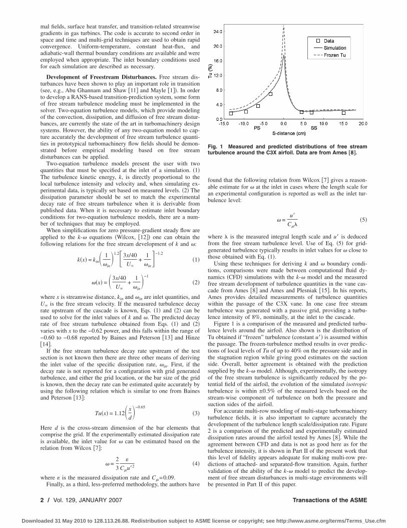
Figure 1 is a comparison of the measured and predicted turbu-lence levels around the airfoil. Also shown is the distribution ofTu obtained if “frozen” turbulence �constant u�� is assumed withinthe passage. The frozen-turbulence method results in over predic-tions of local levels of Tu of up to 40% on the pressure side and inthe stagnation region while giving good estimates on the suctionside. Overall, better agreement is obtained with the predictionsupplied by the k-� model. Although, experimentally, the isotropyof the free stream turbulence is significantly reduced by the po-tential field of the airfoil, the evolution of the simulated isotropicturbulence is within ±0.5% of the measured levels based on thestream-wise component of turbulence on both the pressure andsuction sides of the airfoil.

For accurate multi-row modeling of multi-stage turbomachineryturbulence fields, it is also important to capture accurately thedevelopment of the turbulence length scale/dissipation rate. Figure2 is a comparison of the predicted and experimentally estimateddissipation rates around the airfoil tested by Ames �8�. While theagreement between CFD and data is not as good here as for theturbulence intensity, it is shown in Part II of the present work thatthis level of fidelity appears adequate for making multi-row pre-dictions of attached- and separated-flow transition. Again, furthervalidation of the ability of the k-� model to predict the develop-ment of free stream disturbances in multi-stage environments willbe presented in Part II of this paper.

Fig. 1 Measured and predicted distributions of free streamturbulence around the C3X airfoil. Data are from Ames †8‡.

2 / Vol. 129, JANUARY 2007 Transactions of the ASME


Modeling Pre-Transitional Boundary Layers. Moss and Old-field �16� concluded from their experimental study of the effectsof turbulence level and length scale on heat transfer in laminarboundary layers that, “accurate prediction of heat transfer en-hancement due to free stream turbulence is not possible using theturbulence level alone.” Considering Reynolds’ analogy, it seemsthat accurate predictions of quasi-laminar thermal and momentumboundary layers cannot be obtained without attention to turbu-lence length scale �i.e., specific dissipation� as well as intensity.

The importance of capturing turbulence intensity and length-scale effects on laminar boundary layers was emphasized byBoyle et al. �17�, where the authors developed a model that con-siders both turbulence level and length scale to increase turbulentviscosity above zero in laminar regions to account for what theyrefer to as “turbulence enhancement.” Boyle and co-workers re-ported a “noticeable” improvement in spatially averaged laminar-region heat transfer predictions using their model, but no modeltested produced accurate local heat load levels. Similarly, Roachand Brierley �18� point to the importance of modeling the effectsof turbulence level and length scale on pre-transitional boundarylayers. However, the authors assumed that the integral quantitiesof quasi-laminar boundary layers are the same as the equivalentpurely laminar �Tu=0� boundary layer. Sharma et al. �19� re-viewed experimental evidence that turbulence from upstreamrows imparts a significant influence on the pre-transitional bound-ary layers on turbine airfoils. Additionally, the importance of cap-turing the effects of free stream turbulence on laminar boundarylayers has been identified in experimental studies of convectiveheat transfer rates by Ames �20� and Van Fossen et al. �21�.

The phenomenon of a quasi-laminar boundary layer is demon-strated in the cascade heat transfer data of Arts et al. �22�. Figure3 is a plot of measured heat transfer distributions from Arts et al.�22� with nominal inlet free stream turbulence levels of 1% and6%. Additional flow conditions for both data sets in Fig. 3 wereRec=1�106 and Mexit=0.77, where Rec is Reynolds numberbased on true chord. Heat transfer augmentations in the leading-edge and pressure-side regions of the airfoil of up to approxi-mately 50% are evident. Given that the only difference betweenthe two conditions is the turbulence level, the enhanced energytransfer across the quasi-laminar boundary layer in the high Tucase is primarily due to the penetration of free stream turbulenceinto the laminar boundary layer.

The data from Arts et al. �22� were employed to assess variousmethods for modeling quasi-laminar boundary layers. Uniformsurface-temperature conditions were held for each of the simula-tions, and this was consistent with the measurements. CFD simu-lations �Fig. 3� were run fully laminar on both the suction and

pressure sides of the airfoil employing common modificationsfrom literature to simulate laminar regions. One such techniquetested, which is commonly employed in transitional RANS simu-lations, involves setting the eddy viscosity, �T, from the turbu-lence model to zero within laminar regions. Also tested was thetechnique reported by Schmidt and Patankar �23� in which theproduction term in the k equation is set to zero in laminar regions.

The heat transfer distribution predicted by setting the eddy vis-cosity equal to zero with Tu=6% is shown in Fig. 3. The resultsfor this simulation duplicate the convective heat-load distributionfrom a purely laminar simulation �not shown�. Results from set-ting the production of k equal to zero with Tu=6%, shown in Fig.3, indicate only a slight increase in the predicted heat-load levelsaround the airfoil compared to the prediction with �T=0. Fromthese simulations it is concluded that neither method for modelinglaminar flow with elevated free stream turbulence accurately pre-dicts the wall gradients of the quasi-laminar boundary layer. Sub-sequently, a model was developed based on studies performedwith the data of Arts et al. �22�. Results based on the new modelfor quasi-laminar boundary layers are shown in Fig. 4 and labeledas “QL model.” As seen in this figure, the results from the QLmodel are more accurate in quasi-laminar regions than the resultsshown in Fig. 3. The current method is based on physical reason-ing which links the production terms in the k and � equations to

Fig. 2 Comparison of measured and predicted turbulence dis-sipation around the C3X airfoil. Data are from Ames †8‡.

Fig. 3 Measured convective heat transfer coefficient distribu-tions from Arts et al. †22‡ and CFD predictions run with fullylaminar boundary layers

Fig. 4 Results from CFD simulations run with the QL modelfor capturing pre-transitional quasi-laminar boundary layers

Journal of Turbomachinery JANUARY 2007, Vol. 129 / 3


the concept of self-sustaining turbulence in turbulent boundarylayers. The analogy is drawn that in laminar regions of the bound-ary layer, where disturbances are damped by the action of viscos-ity, the production of both k and � should be negligible. Implicitin this analogy is that the eddy viscosity in a quasi-laminar bound-ary layer is independent of the mean strain. Minimizing the pro-duction terms in the k and � equations, in contrast to setting �T=0, allows for the convection and diffusion of free stream turbu-lence into quasi-laminar �QL� boundary layers. For the lengthscales �i.e., dissipation rates� and turbulence intensities present inthe data of Arts et al. �22�, the QL model was found to captureconvective heat loads to within ±10% in quasi-laminar regions forall conditions reported.

Additional testing of the QL model was performed with thecascade data of Ames �8� with similar accuracy for convectiveheat loads for levels of Tu up to 12% from a simulated combustor�Praisner et al. �24��. Additionally, predictions of stagnation-pointheat transfer levels from the QL model are within ±10% of thecorrelation of Van Fossen et al. �21� for a range ofturbomachinery-specific turbulence and dissipation levels.

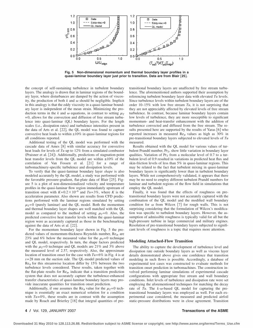
To verify that the quasi-laminar boundary layer shape is alsomodeled accurately by the QL model, a study was performed withthe favorable pressure-gradient, flat-plate data of Blair �25�. Fig-ure 5 is a plot of non-dimensionalized velocity and temperatureprofiles in the quasi-laminar flow region immediately upstream oftransition onset with K=0.2�10−6 and Tu=3%, where K is theacceleration parameter. Also shown are results from CFD predic-tions performed with the laminar regions simulated by setting�T=0 �purely laminar� and the QL model. Both the momentumand thermal boundary layer shapes are well matched with the QLmodel as compared to the method of setting �T=0. Also, thepredicted convective heat transfer levels within the quasi-laminarregion were as accurately captured as those in the benchmarkingagainst the data of Arts et al. �22�.

For the momentum boundary layer shown in Fig. 5 the pre-dicted values of momentum-thickness Reynolds number, Re�, are23% and 6% below the measured value for the �T=0 techniqueand QL model, respectively. In turn, the shape factors predictedwith the �T=0 technique and QL models are 21% and 3% abovethe measured level of 2.57, respectively. Also, the approximatelocation of transition onset for the case with Tu=6% in Fig. 4 is ats=28 mm on the suction side. The QL-model predicted values ofRe� for this streamwise location differ by 15% between the twoturbulence levels considered. These results, taken together withthe flat-plate results for Re�, indicate that a transition predictionsystem that does not accurately capture the turbulence-enhancedtransfer characteristics of quasi-laminar boundary layers may pro-vide inaccurate quantities for transition onset prediction.

Additionally, if one assumes the Re� value for the �T=0 tech-nique is essentially an exact numerical solution for a conditionwith Tu=0%, these results are in contrast with the assumptionmade by Roach and Brierley �18� that integral quantities of pre-

transitional boundary layers are unaffected by free stream turbu-lence. The aforementioned authors supported their assumption byreferencing turbulent boundary layer data with elevated Tu levels.Since turbulence levels within turbulent boundary layers are of theorder 10–15% with low free stream Tu, it is not surprising thatthey are not appreciably affected by elevated levels of free streamturbulence. In contrast, because laminar boundary layers containlow levels of turbulence, they are more susceptible to significantmomentum- and heat-transfer enhancement with the addition ofturbulence convected and diffused from the free stream. The re-sults presented here are supported by the results of Yaras �6� whoreported increases in measured Re� values as high as 30% inpre-transitional boundary layers subjected to elevated levels of Tumeasured.

Results obtained with the QL model for various values of tur-bulent Prandtl number, PrT, show little variation in boundary layerqualities. Variation of PrT from a molecular level of 0.7 to a tur-bulent level of 0.9 resulted in variations in predicted heat flux andskin-friction levels of less than 5% in quasi-laminar regions. Thismay be related to the fact that turbulent mixing in quasi-laminarboundary layers is significantly lower than in turbulent boundarylayers. While not comprehensively validated, it appears that theremay be no need to employ different turbulent Prandtl numbers forlaminar and turbulent regions of the flow field in simulations thatemploy the QL model.

Finally, it was found that the effects of roughness on pre-transitional boundary layers were not accurately captured with thecombination of the QL model and the modified wall boundarycondition for � from Wilcox �7� for rough walls. This is notsurprising considering that the formulation of Wilcox’s modifica-tion was specific to turbulent boundary layers. However, the as-sumption of admissible roughness is typically valid for all but thehigh-pressure turbine in large commercial and military engines.Resolution of pre-transitional boundary layers subjected to signifi-cant levels of roughness is a topic that requires more attention.

Modeling Attached-Flow TransitionThe ability to capture the development of turbulence level and

dissipation rate outside boundary layers as well as viscous layerdetails demonstrated above gives one confidence that transitionmodeling in such flows is possible. Accordingly, a database ofexperimental test cases was constructed to evaluate methods fortransition onset prediction in turbomachines. The construction in-volved performing laminar simulations of experimental cascadeconfigurations with appropriate free stream and wall boundaryconditions. Inlet levels of turbulence and dissipation rate were setemploying the aforementioned techniques for matching the decayrate of Tu. The k-�-based QL model for capturing the pre-transitional boundary layers was employed as well. For each ex-perimental case considered, the measured and predicted airfoilstatic-pressure distributions were in close agreement. Transition

Fig. 5 Non-dimensional momentum and thermal boundary layer profiles in aquasi-laminar boundary layer just prior to transition. Data are from Blair †25‡.



onset was considered to occur in the data sets where wall-gradientquantities first began to deviate from fully laminar simulations.Only cascade geometries of turbomachinery-specific airfoils wereconsidered, and both open-literature and in-house data were usedto build the database of 57 cases. The 57 cases themselves con-sisted of seven different geometries tested in experiments withvarious boundary conditions.

Review of Models for the Onset of Transition. The most suc-cessful physical model for the transition process is that due toEmmons �26�, Schubauer and Klebanoff �27�, and Narasimha�28�. In this model, transition is considered to be the result of therandom formation of “spots” of turbulence in the boundary layerover some finite region in the streamwise direction. These turbu-lent spots grow as they convect downstream, and the intermittency�i.e., the fraction of time the flow is turbulent� increases in thestreamwise direction until the entire surface is covered with them.At that point, the boundary layer is considered fully turbulent.

The foregoing would suggest that an assessment of the effectsof various flow field parameters on transition must be an evalua-tion of the way in which they affect the formation and subsequentgrowth of turbulent spots and/or wake-induced turbulent strips.Several authors have conducted experimental studies in that re-gard �e.g., Clark et al. �29�, Gostelow et al. �30�, and Halstead etal. �31��, and others �e.g., Chen and Thyson �32�, Dey andNarasimha �33�, and Solomon et al. �34�� have incorporated infor-mation on turbulent-spot formation and kinematics into integralmethods for calculating intermittency and, by extension through a“linear combination model” after Dhawan and Narasimha �35�,skin friction. Still others �e.g., Suzen and Huang �36� and Steelantand Dick �37�� have made use of the “universal” intermittencydistribution to derive transport equations for intermittency that aresolved alongside the RANS equations or used some combinationof the correlations of Abu-Ghannam and Shaw �11�, Drela �38�,and Solomon et al. �34� to evaluate intermittency �e.g., Gier et al.�39�, Thermann et al. �40�, Roux et al. �41�, and Roberts and Yaras�42�� through transition. Subsequently, some of the same authorsmodified the calculated eddy viscosity according to the fraction oftime the flow is predicted to be turbulent through the transitionzone. As previously stated, pre-transitional boundary layers withelevated Tu levels may not be adequately modeled by setting �Tequal to zero upstream of transition onset.

The review article of Mayle �1� spurred renewed interest in theideas of Emmons �26� and Narasimha �28� for the prediction oftransition in turbomachines, and much of the recent work de-scribed above followed recommendations from that paper closely.In particular, the concept of the universal intermittency distribu-tion as described in detail by Narasimha �43� has been used tobuild correlations for transition onset �Mayle �1��, as well asturbulent-spot generation rates and transition length �Fraser et al.�44� and Gostelow et al. �30��.

At the root of many correlations used to predict transition onsetis the F�� technique of Narasimha �43�, whereby measuredstreamwise variations of intermittency, , are plotted in the form

F�� = �− ln�1 − ��1/2 �6�

Narasimha �28� first proposed that all turbulent spots are formedrandomly in time and spanwise location at a single streamwisestation in the flow. Under that hypothesis, which is now knowngenerally as “concentrated breakdown,” Eq. �6� becomes

F�� = � n

U��1/2

�x − xt� �7�

for constant-velocity flow along a flat plate. In Eq. �7�, xt is thestreamwise location where all spots are formed, n is the number ofspots formed at that position per unit time and per unit spanwisedistance, U� is the free stream velocity, is Emmons �26� non-dimensional spot-propagation parameter, and x is a location on the

flat-plate surface further downstream than xt.Dhawan and Narasimha �35� also showed that variations of

intermittency through the transition zone possess a high degree ofsimilarity if the streamwise distance is suitably non-dimensionalized. They demonstrated that the transitional intermit-tency variations from a number of experiments collapsed on asingle curve when the streamwise distance was represented by

� =x − xt

x75 − x25�8�

where x75 and x25 are the streamwise positions where the intermit-tency is 0.75 and 0.25, respectively. The same authors alsoshowed that the available intermittency data were well representedby the equation

= 1 − e−0.412�2�9�

Equation �9� has become known as the universal intermittencydistribution �Narasimha �45,46��. Like Eq. �7�, Eq. �9� is a conse-quence of the assumption of concentrated breakdown as applied tothe transition model of Emmons �26� in constant velocity, flat-plate flow.

Many authors have shown that it is possible to linearize inter-mittency distributions using Eqs. �6� and �7� and, consequently, toplot the data in the universal form of Eq. �9� �e.g., Owen �47��.This is true even under conditions of changing pressure gradientand/or free stream velocity �Sharma et al. �48�, Gostelow et al.�30�, and Fraser et al. �44��. As an illustration of this phenomenon,representative data from Clark �49� are plotted in Fig. 6. Experi-mental intermittency distributions for flat-plate flows under bothfavorable and adverse pressure gradient conditions are plotted,and both agree with the universal curve very well. This is surpris-ing in the case with the favorable pressure gradient since the localvelocity varies by a factor of more than 6.7 over the streamwisedistance represented in the figure. Note that both the spot shapeparameter and the free stream velocity itself are considered con-stant and brought outside an integrand in the derivation of Eq. �7�,and neither of these assumptions is valid in the experiment ofClark �49�. Intermittency variations predicted with a time-marching simulation of the transition zone like that described byNarasimha �50� are also plotted in Fig. 6. These predicted inter-mittency distributions are taken along the centerline of a flat-plateflow at Mach 0.5. Spot propagation parameters were as measuredby Clark et al. �29�, and three different distribution functions forspot generation were considered. The universal curve fits the pre-

Fig. 6 A comparison between the “universal” curve ofNarasimha †43‡ and both experimental data and simulationsfrom Clark †49‡



dicted intermittency distributions very well, not just when concen-trated breakdown prevails, but also for both a bivariate normal �instreamwise and spanwise directions� spot generation function anda point source located off the plate centerline.

Observations like those presented here with respect to the uni-versal curve are not new �see, e.g., Dhawan and Narasimha �35��.In more recent times Mayle �1� used the F�� technique to de-velop a correlation for transition onset, where onset was taken tobe the x intercept of the F�� plot. Also, correlations for length aswell as turbulent-spot generation rates under a variety of flowconditions �Mayle �1�, Gostelow et al. �30�, and Fraser et al. �44��have been derived. From the discussion above, it does not followthat if it is possible to linearize experimental data by plottingF��, then the transition is consistent with a flat-plate flow under-going transition via a concentrated breakdown of the laminarboundary layer. When the current database for attached-flow tran-sition onset is compared to one such correlation from Mayle �1�,as in Fig. 7, there is considerable scatter. Testing against the da-tabase revealed a success rate of approximately 50% in predictingonset within 10% of the measured location in terms of surfacedistance. Also, transition onset typically occurs at lower Reynoldsnumbers than predicted by the Mayle �1� relation. Similar resultsto those in Fig. 7 are reported by Simon and Ashpis �4� for com-parisons made between data and the Mayle �1� correlation. In lightof these findings, it might be better to develop correlations fortransition onset and turbulent-spot production rates, for example,from direct measurements like those first reported by Hofeldt �51�.Such direct measurements are difficult, however, and little dataare available at present to create such correlations.

Both Tani �52� and Reshotko �53� review a number of modelsthat are not based on the concept of universal intermittency, andthey both point out that one of the first was due to Liepmann �54�.Many authors refer to Liepmann �55� as the source of this idea,but the 1945 publication is the correct one. Liepmann supposedthat transition onset occurs when the local Reynolds stress in theperturbed laminar boundary layer equals the local friction veloc-ity. Liepmann’s idea has been recast and used by others. For ex-ample, Van Driest and Blumer �56� correlated the local vorticityReynolds number, which like the friction velocity depends on thenormal gradient of streamwise velocity in two dimensional �2D�flow, at transition onset with free stream turbulence and pressuregradient. Recently, Mayle and Schulz �57� referred to the formu-lation of Liepmann’s criterion due to Sharma et al. �48� as appro-priate for transition onset. Sharma et al. �48� argued that the local

Reynolds stress itself depends on the local root mean square ofstreamwise velocity perturbations and stated that transition onsetoccurs when

u�

u* = 3.0 �10�

based on experimental data related to a turbine airfoil suction-sideflow field. In Eq. �10�, u* is the local friction velocity and u� is thefluctuating component of the local streamwise velocity. Liepmann�54� argued the same case based on his own experimental data.Following Liepmann’s analysis and recasting his correlation in theform of Eq. �10� results in a constant on the right-hand sideequal to 7.5 rather than 3. In addition, Roach and Brierley �18�report that the constant in Eq. �10� varies from 3.0 to 7.4 for theERCOFTAC T3 test cases.

If one assumes that u� within the quasi-laminar boundary layeris modeled to a reasonable level of accuracy with the QL model, itmight be possible to predict transition onset based on a relationlike that in Eq. �10�. In Fig. 8 the quantity u� /u*, evaluated attransition onset, is plotted for all cases in the current database. Forcomparison both the constants of Sharma et al. �48� and Liepmann�54� are also plotted. Transition onset seems to occur at muchlower levels of u� /u* than those indicated by Sharma et al. �48�and Liepmann �54� over the entire database.

The poor correlation of the database in Fig. 8 may likely be aresult of the assumption of isotropic turbulence within the quasi-laminar boundary layer inherent in the QL model. Also, one notesthat the studies of Sharma et al. �48� and Liepmann �54� predatethe use of conditional sampling techniques for boundary-layermeasurements �see, e.g., Suder et al. �58� and Kim et al. �59��. So,it could be that the local rms of velocity fluctuations in the bound-ary layer was largely influenced by the passage of turbulent spotsover the fixed hot wires in the experiments of both Liepmann �54�and Sharma et al. �48�. As such, the criteria represented by Eq.�10� might be more indicative of turbulent-spot detection than ofthe state of a quasi-laminar boundary layer at transition onset. Theforegoing argument is supported by the results of a simple calcu-lation. Consider a boundary layer profile undergoing transition tobe a linear combination of laminar and fully turbulent profilesweighted on the intermittency, as suggested first by Dhawan andNarasimha �35�, and let onset occur in a Blasius boundary layeron a flat plate at a local streamwise Reynolds number of 250,000.

Fig. 7 A comparison between the current database forattached-flow transition onset and the correlation of Mayle †1‡

Fig. 8 A comparison between the transition onset criteria ofLiepmann †54‡, Sharma et al. †48‡, and Mayle and Schulz †57‡and the current attached-flow database



If one represents the turbulent profiles by a 1/7th power law andpresumes there is no change in boundary layer thickness at tran-sition onset �strictly speaking, there can be no change in the localmomentum thickness�, then at y+=25, the local rms becomesabout three times the local friction velocity if the intermittency is10%. This is in keeping with the results of Sharma et al. �48�. Inany regard, the results shown in Fig. 8 suggest that with the cur-rent modeling of pre-transitional boundary layers, accurateRANS-based transition predictions cannot be obtained with amodel of the type in Eq. �10�.

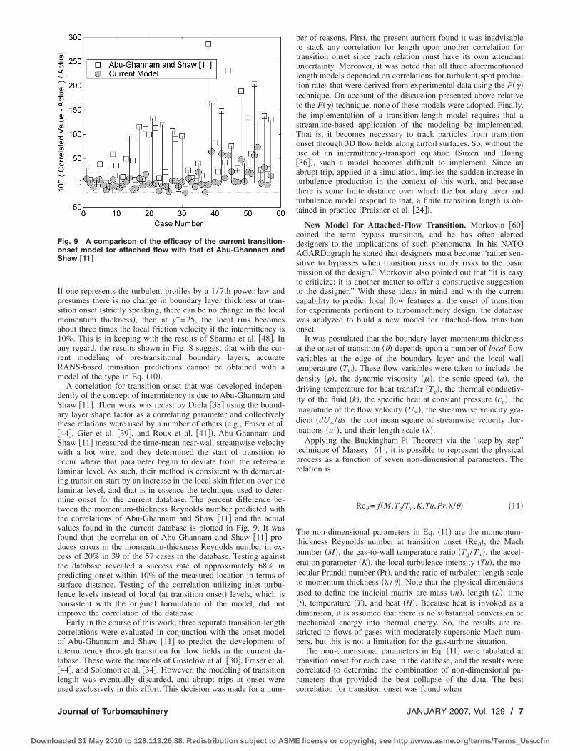
A correlation for transition onset that was developed indepen-dently of the concept of intermittency is due to Abu-Ghannam andShaw �11�. Their work was recast by Drela �38� using the bound-ary layer shape factor as a correlating parameter and collectivelythese relations were used by a number of others �e.g., Fraser et al.�44�, Gier et al. �39�, and Roux et al. �41��. Abu-Ghannam andShaw �11� measured the time-mean near-wall streamwise velocitywith a hot wire, and they determined the start of transition tooccur where that parameter began to deviate from the referencelaminar level. As such, their method is consistent with demarcat-ing transition start by an increase in the local skin friction over thelaminar level, and that is in essence the technique used to deter-mine onset for the current database. The percent difference be-tween the momentum-thickness Reynolds number predicted withthe correlations of Abu-Ghannam and Shaw �11� and the actualvalues found in the current database is plotted in Fig. 9. It wasfound that the correlation of Abu-Ghannam and Shaw �11� pro-duces errors in the momentum-thickness Reynolds number in ex-cess of 20% in 39 of the 57 cases in the database. Testing againstthe database revealed a success rate of approximately 68% inpredicting onset within 10% of the measured location in terms ofsurface distance. Testing of the correlation utilizing inlet turbu-lence levels instead of local �at transition onset� levels, which isconsistent with the original formulation of the model, did notimprove the correlation of the database.

Early in the course of this work, three separate transition-lengthcorrelations were evaluated in conjunction with the onset modelof Abu-Ghannam and Shaw �11� to predict the development ofintermittency through transition for flow fields in the current da-tabase. These were the models of Gostelow et al. �30�, Fraser et al.�44�, and Solomon et al. �34�. However, the modeling of transitionlength was eventually discarded, and abrupt trips at onset wereused exclusively in this effort. This decision was made for a num-

ber of reasons. First, the present authors found it was inadvisableto stack any correlation for length upon another correlation fortransition onset since each relation must have its own attendantuncertainty. Moreover, it was noted that all three aforementionedlength models depended on correlations for turbulent-spot produc-tion rates that were derived from experimental data using the F��technique. On account of the discussion presented above relativeto the F�� technique, none of these models were adopted. Finally,the implementation of a transition-length model requires that astreamline-based application of the modeling be implemented.That is, it becomes necessary to track particles from transitiononset through 3D flow fields along airfoil surfaces. So, without theuse of an intermittency-transport equation �Suzen and Huang�36��, such a model becomes difficult to implement. Since anabrupt trip, applied in a simulation, implies the sudden increase inturbulence production in the context of this work, and becausethere is some finite distance over which the boundary layer andturbulence model respond to that, a finite transition length is ob-tained in practice �Praisner et al. �24��.

New Model for Attached-Flow Transition. Morkovin �60�coined the term bypass transition, and he has often alerteddesigners to the implications of such phenomena. In his NATOAGARDograph he stated that designers must become “rather sen-sitive to bypasses when transition risks imply risks to the basicmission of the design.” Morkovin also pointed out that “it is easyto criticize; it is another matter to offer a constructive suggestionto the designer.” With these ideas in mind and with the currentcapability to predict local flow features at the onset of transitionfor experiments pertinent to turbomachinery design, the databasewas analyzed to build a new model for attached-flow transitiononset.

It was postulated that the boundary-layer momentum thicknessat the onset of transition �� depends upon a number of local flowvariables at the edge of the boundary layer and the local walltemperature �Tw�. These flow variables were taken to include thedensity ��, the dynamic viscosity ��, the sonic speed �a�, thedriving temperature for heat transfer �Tg�, the thermal conductiv-ity of the fluid �k�, the specific heat at constant pressure �cp�, themagnitude of the flow velocity �U��, the streamwise velocity gra-dient �dU� /ds, the root mean square of streamwise velocity fluc-tuations �u��, and their length scale ��.

Applying the Buckingham-Pi Theorem via the “step-by-step”technique of Massey �61�, it is possible to represent the physicalprocess as a function of seven non-dimensional parameters. Therelation is

Re� = f�M,Tg/Tw,K,Tu,Pr,�/�� 11�

The non-dimensional parameters in Eq. �11� are the momentum-thickness Reynolds number at transition onset �Re��, the Machnumber �M�, the gas-to-wall temperature ratio �Tg /Tw�, the accel-eration parameter �K�, the local turbulence intensity �Tu�, the mo-lecular Prandtl number �Pr�, and the ratio of turbulent length scaleto momentum thickness �� /��. Note that the physical dimensionsused to define the indicial matrix are mass �m�, length �L�, time�t�, temperature �T�, and heat �H�. Because heat is invoked as adimension, it is assumed that there is no substantial conversion ofmechanical energy into thermal energy. So, the results are re-stricted to flows of gases with moderately supersonic Mach num-bers, but this is not a limitation for the gas-turbine situation.

The non-dimensional parameters in Eq. �11� were tabulated attransition onset for each case in the database, and the results werecorrelated to determine the combination of non-dimensional pa-rameters that provided the best collapse of the data. The bestcorrelation for transition onset was found when

Fig. 9 A comparison of the efficacy of the current transition-onset model for attached flow with that of Abu-Ghannam andShaw †11‡



Re� = A�Tu�

��B

�12�

where A and B are constants equal to 8.52 and −0.956, respec-tively. The entire database is plotted in Fig. 10. Equation �12�implies that the local momentum thickness at transition onset is afunction of only one non-dimensional parameter that is a productof two of the basic non-dimensional parameters derived directlyfrom the step-by-step method of Massey �61�.

An ability to determine the edge of the boundary layer in arobust manner is an important aspect of transition modeling tech-niques based on integral and edge quantities. The edge of theboundary layer was taken to be the distance from the wall atwhich the local vorticity dropped to 1% of the maximum value inthe O grid at that streamwise grid location. This method, reportedby Michelassi et al. �62�, provides a robust and accurate edgedetection technique for laminar boundary layers. Variations in thepercentage of the maximum vorticity used to define the boundarylayer edge between 0.8% and 1.8% resulted in variations in thecoefficient of correlation of the least-squares fit for Eq. �12� on therange from 0.95 to 0.96.

As seen in Table 1, all the non-dimensional parameters, savethe molecular Prandtl number, varied markedly at transition onsetover this database. For example, transition onset occurred underboth favorable and adverse pressure gradients. The strength of thepressure gradients covers the range from above relaminarization�K�3�10−6� on the favorable side through Thwaite’s separationcriterion �K Re�

2 −0.09, see White �63�� under decelerating con-ditions. Both adiabatic flows and those with velocity profiles thatwere affected by the temperature dependence of viscosity werepart of the database. Also, the range of Mach numbers coveredincompressible through transonic flows. The local turbulence in-tensity varied by two orders of magnitude, and while the maxi-

mum value may at first consideration seem low, one must remem-ber that the inlet turbulence intensity was much higher. Further,the ratio of local turbulence length scale to momentum thicknessat onset varied by an order of magnitude. Again, the molecularPrandtl number was essentially constant for all points in the data-base.

Physical Significance of the Current Attached-Flow Model.Equation �12� was incorporated into the airfoil design system di-rectly with the factor and power in the equation set equal to 8.52and −0.956, respectively. However, it is possible to recast therelation in such a way that gives insight into its possible physicalsignificance. One notes that the constant B in the relation is veryclose to −1. If that value is accepted, then, after some algebraicmanipulation, Eq. �12� becomes:

100�u�

��2

�� = A1 �13�

where A1 is another constant that may be evaluated directly as themean of values occurring at transition onset in the database. Here,A1 was found to be 7.0±1.1. Note that Eq. �13� implies that tran-sition onset occurs when the ratio of a boundary-layer diffusiontime ��2 /�� to a time scale associated with the large-eddy tur-bulent fluctuations �te=� /u�� becomes a critical value.

It is instructive to consider the implications of Eq. �13� for aBlasius boundary layer undergoing transition. The usual form ofthe laminar diffusion time scale, td, is ��2 /� �see, e.g., Schlichting�64�, and Hofeldt et al. �65�� where � is the thickness where thelocal velocity becomes 99% of the free stream value and � is thefluid density. The ratio of 99% velocity thickness to momentumthickness in a Blasius boundary layer is 5:0.664. Substituting intoEq. �13�, taking A1 equal to 7.0, and rearranging gives

te = 0.25td �14�Now, the time for a Blasius boundary layer to grow to a thickness� is 1 /25th the laminar diffusion time scale �Schlichting �64��. So,transition onset would occur for the Blasius boundary layer whenthe local eddy time scale approached a level associated with agrowth of 6 boundary layer thicknesses. Schlichting �64� givesthe smallest unstable wavelength of a Blasius boundary layer as6�. So, Eq. �14� implies that the onset of bypass transition oc-curs when the local eddy time scale reaches a time scale associ-ated with the wavelength of a Tollmien-Schlichting �TS� wave.

Although one typically does not associate TS activity with by-pass transition, it has been noted by Herbert �66� that the ultimatebreakdown associated with the appearance of “spikes” in hot-wirerecords and the first formation of turbulent spots in natural tran-sition occurs over a length scale of about 1 TS wavelength. Also,Walker and Gostelow �67� have measured frequencies consistentwith TS activity in boundary layers undergoing bypass transitionin adverse pressure gradients. Additionally, Mack �68� noted thatoften TS frequencies persist in boundary layers undergoing natu-ral transition beyond the range of applicability of small distur-bance theory. Volino �69,70� also reported that for separated-flowtransition, TS frequencies were detected for both low and highlevels of Tu. Again, the real implication of this discussion is thatwhen the ratio of the turbulent-eddy time scale to the laminardiffusion time reaches a critical value, bypass transition occurs.Further, the critical value of this ratio is nearly constant over arange of flow conditions consistent with gas-turbine engines.

Modeling Laminar Separation and Turbulent Reattach-ment

“Of all the transition modes, there is none more crucial to com-pressor and low-pressure turbine design and none more neglectedthan separated-flow transition” �Mayle �1��. As attempts are madeto reduce airfoil counts, and hence component cost and weight,airfoil loadings need to increase. Highly loaded airfoils are more

Fig. 10 The current model for the onset of attached-flow tran-sition compared to the database

Table 1 Variation of non-dimensional parameters at transitiononset

Variable Range

Re�73–856

K�106 −1.9 to 4.8KRe�

2 −0.15 to 0.06M 0.05–1.24

Tg /Tw1.0–1.41

Tuonset �%� 0.11–5.09� /� 4.26–66.2Pr 0.71–0.71



prone to experiencing laminar separations �Fig. 11� and stall. Inthe stalled condition profile losses can increase as much as 500%over the case where the separation reattaches to the airfoil. Lami-nar separations occur in the leading-edge, suction-side regions ofcompressors and the aft suction-side regions of low-pressure tur-bine �LPT� airfoils. Airfoil stall causes compressor surge and poorperformance of LPTs at cruise conditions.

If the laminar shear layer formed by a separation transitions toa turbulent state close enough �i.e., in a stream-wise sense� to theseparation location, it typically reattaches to the airfoil surface asa result of turbulent mixing that entrains high-momentum fluidinto the near-wall region. This scenario is schematically depictedin Fig. 11�a�. However, if transition of the shear layer occurssufficiently far downstream of separation, the layer typically doesnot reattach, resulting in a stalled condition as shown in Fig.11�b�. It is therefore critical that a design system be capable ofpredicting the existence of a laminar separation and whether ornot the laminar separation will reattach.

As a first step in developing a transition modeling capability forseparated flow, a proof-of-concept study was executed with thegoal of determining if a separated-flow transition model could beeffectively implemented in a RANS code. For this study, CFDsimulations of cascade experiments were run with imposed abrupttrips, set according to experimental hot-film data. Figure 12 is aplot of separation and reattachment locations as a function of exitReynolds number for a cascade airfoil with Tu=5%. The totalsuction-side surface length of the airfoil for this case was37.1 mm, and both experimental and computational results areshown in Fig. 12.

It can be seen in Fig. 12 that the separation and reattachmentlocations from simulations utilizing the QL model for the pre-transitional boundary layers are in close agreement with the dataat all but the lowest simulated Reynolds number. The deviationfrom the data at the lowest Reynolds number is a result of stalloccurring in the simulation and subsequent unsteadiness in thesteady simulation. For a Reynolds number of 1.5�105 a simula-tion was also run with the turbulent viscosity set to zero in laminarregions and the results are also plotted in Fig. 12. For this simu-lation the separation location occurs upstream of the measuredlocation. This is consistent with the quasi-laminar boundary layershape, and hence near-wall momentum, not being accurately mod-eled by setting �T=0. The calculated loss levels from the simula-tions shown in Fig. 12 were in good agreement with the measuredvalues. The conclusion of this study was that the RANS code with

abrupt trips and some form of modeling for quasi-laminar, pre-transitional boundary layers would provide an accurate frameworkfor separated-flow transition modeling.

So, in addition to the attached-flow transition studies, a CFD-supplemented database of laminar separations with turbulent reat-tachment was constructed based on 47 in-house and open-literature experimental cascade data sets. The test cases for theseparated-flow database include laminar separations with turbu-lent reattachment on both compressor- and turbine-specificgeometries. Some of the data sets included in the database arefrom airfoils on the verge of stall. Like the attached-flow database,the separated-flow database covers a significant range ofturbomachinery-specific flow parameters.

Review of Models for the Onset of Separated-FlowTransition. One common method for predicting the transition lo-cation of a near-wall bounded shear layer involves the use of acorrelation that was developed for attached-flow transition such aseither the Mayle �1� or Abu-Ghannam and Shaw �11� model.These models rely on a non-dimensional boundary layer thickness�Re� or shape factor� for the prediction of transition onset andwere developed with data for attached-flow transition. As depicted

Fig. 11 Schematic representation of suction-side, laminar-separation characteristics showingboth reattached „a… and stalled „b… conditions

Fig. 12 Measured and predicted separation and reattachmentlocations. Transition was specified in the simulations based ondata.



in Fig. 11, in the separated region, the only attached boundarylayer that exists is the reverse-flow boundary layer within theseparation bubble. The primary issue with employing an attached-flow transition model in a region where the flow is separated isthat the physical significance of Re� fundamentally changes oncethe boundary layer separates.

A rather unique model for the prediction of separated-flow tran-sition was reported by Roberts �71�, in which the distance fromthe separation location to the shear layer transition location �L inFig. 11� is related to free stream turbulence quantities. This modelis unique in that it considers both turbulence intensity and lengthscale in predicting separated-flow transition onset. Figure 13 is acomparison between predictions performed with the model ofRoberts �71� and the separated-flow database. Plotted in this figureis Reynolds number based on L versus the local “turbulence fac-tor” which is defined as TF=Tu�C /��0.2, where C is the airfoilchord. The highest level of turbulence factor considered in thedevelopment of the Roberts �71� model was approximately 0.06.This model was developed for external flows with low free streamturbulence levels � 0.2% �. The only database cases that are wellcorrelated by this model are the cases in which Tu 0.6% �Fig.13�. The Roberts model �71� does not correlate database caseswith Tu�0.6% well enough for implementation in a design sys-tem. Additionally, alteration of the model by leaving out thelength scale in the calculation of TF, as suggested as a possiblemodification by Roberts �71�, did not improve the correlation ofthe database.

Other separated-flow transition models have been reported byWalker �72�, Mayle �1�, and Hatman and Wang �73�. These mod-els relate separation length to the conditions of the laminar bound-ary layer at the separation location. RANS-based simulations em-ploying models of this type have proven to be at least trendaccurate in the prediction of separated transition �see, e.g., Volino�69,70� and Houtermans et al. �74��. The separated-flow transitiondatabase was employed to test the models of Mayle �1� for “long”and “short” bubbles and a comparison of the predicted and mea-sured bubble lengths is shown in Fig. 14. It can be seen in thisfigure that neither the long- nor the short-bubble model providessufficient accuracy for design purposes. Similar results were ob-tained for comparisons between the models due to Walker �72�and Hatman and Wang �73� and the separated-flow database.These results are supported by Volino �69,70� who reported thatthe correlations of Hatman and Wang �73�, Mayle �1�, and Daviset al. �75� give “rough” estimates for the transition behavior of hisexperimental test cases.

New Model for Separated-Flow Transition. In RANS-based

simulations the authors believe that the multi-moded �1� nature oftransition is best captured by employing two separate models forattached and separated transition. So, following the body of ma-terial concerning models for separated-flow transition summarizedabove, a new model has been developed based on the separated-flow database. The same dimensional-analysis technique used forthe attached-flow model was employed in the development of thismodel. The best correlation of the database was obtained when thelength of the bubble was related to the state of the boundary layerat separation. The form of the current model is:

L

Ssep= CRe�−sep

D �15�

where C and D are constants equal to 173.0 and −1.227, respec-tively, L is the distance between separation and transition onset,and Ssep is the surface distance from the stagnation point to theseparation location.

The separated-flow database is shown in Fig. 15 along with thecurrent transition model �Eq. �15��. The reasonably good correla-tion of the database with the recasting of Walker’s original idea�72� supports the assertion that for viscously dominated, near-wallbounded separations, the bubble size scales on the state of theboundary layer at separation. While Eq. �15� does not explicitlycontain turbulence quantities, they are still important in the deter-mination of Re� at the separation location if a model, such as the

Fig. 13 A comparison between the separated-flow transitionmodel of Roberts †71‡ and the separated-flow transitiondatabase

Fig. 14 A comparison between the separated-flow transitionmodels of Mayle †1‡ and the separated-flow transition database

Fig. 15 The current model and database for separated-flowtransition. The model with a conservative shift is also shown.



current QL model, is employed to capture the effects of freestream turbulence on the pre-separation quasi-laminar boundarylayer. Additionally, it should be noted that Eq. �15� was imple-mented in the design system in a conservative fashion by setting Cat a level 20% higher than the least-squares-fit value plotted onFig. 15 as “current model.” This conservatively defined correla-tion is also plotted in Fig. 15 as “shifted model” and represents anupper bound for bubble sizes in the database.

If modeling of the effects of free stream turbulence on the pre-transitional/separation boundary layers is not used in conjunctionwith the attached- and separated-flow models presented here, aconservative predictive system for low-Reynolds number sepa-rated flows results. As demonstrated earlier �Figs. 5 and 12�,onset/separation values of Re� are under-predicted �by 15% ormore� when quasi-laminar effects are not modeled. This, takenwith the inverse relation between Re� and the length of the sepa-rated region presented in Eq. �15�, results in an over prediction ofbubble length and hence a conservative prediction of the perfor-mance of an airfoil with separated flow. That is, the analyticallydetermined stall Reynolds number is larger when Eq. �15� is usedin the absence of pre-transitional modeling, and thus airfoils de-signed in that fashion may have better than predicted Reynolds-lapse characteristics. Such was the case for the L1M airfoil de-signed at AFRL and tested by Bons et al. �76�. The designers ofthe L1M used an entirely different design system than that em-ployed in this study and made use of Eq. �15� without the benefitof pre-transitional modeling. The L1M airfoil had a designZweifel coefficient of 1.34, and it was stall free for the range ofReynolds numbers tested in the experiment, as predicted. Thelowest Reynolds number achieved in the experimental verificationof the airfoil performance was 20,000. At that Reynolds number,the suction-side bubble was predicted to close at 92% of the axialchord, whereas the measured re-attachment was at approximately80%.

In his experimental assessment of the Pack B airfoil, Volino�69,70� reported that boundary layer reattachment occurs essen-tially simultaneously with transition onset for separated flow tran-sition. This supports the assertion made by Lou and Hourmouzia-dis �77� that the transition length is very short because of the lackof wall damping in the shear layer. Also, Walker et al. �78� re-ported that abrupt transition is a relatively �compared totransition-length models for separated flow� realistic model of thetransition region in laminar separation bubbles. So, as in the caseof attached-flow transition, abrupt transition is assumed for theimplementation of the current separated-flow model. Validation ofthe many assumptions involved in the development of both mod-els as well as their implementation is reported in Part II of thiswork.

Physical Significance of the Current Separated-Flow Model.While the concept of long and short bubbles has been discussed inliterature relating to separated-flow transition for many decades,the present results suggest that the concept may not be importantin turbomachinery configurations. The present database is in con-flict with reports of Hatman and Wang �73� and Houtermans et al.�74� where the existence of two bubble regimes seems evidentfrom data. In the current database, no long bubbles, that signifi-cantly alter airfoil pressure distributions, were found that alsoreattached to the airfoil. In other words, separations that do notreattach, and hence alter the turning characteristics and loadingsof airfoils, are not referred to as bubbles here as they are notclosed. Large reattaching bubbles that significantly alter pressuredistributions are possible on flat-plate configurations such as thatemployed by Hatman and Wang �73� if reattachment occursdownstream of the simulated trailing edge. Therefore, their corre-lation may still be useful in predicting where the laminar shearlayer transitions downstream of an airfoil trailing edge. Thepresent database shows a continuous distribution of separationbehavior up to the point of stall. This is consistent with the resultsof Houtermans et al. �74� for their short bubble regime. The data

regarded as reflecting long bubble behavior by Houtermans et al.�74� is here interpreted as arising from stalled conditions. So, theauthors believe that the short bubble regime primarily describesseparation behavior with reattachment. In this work, if separated-flow transition onset is predicted to occur downstream of the air-foil trailing edge, then the airfoil is run fully laminar.

ConclusionsThe ability to model accurately the development of free stream

disturbances has been shown to be an important aspect of anytransition modeling capability. Evidence has been presented thatcapturing the effects of free stream turbulence on pre-transitionalboundary layers may enhance the accuracy of empiricisms usedfor the prediction of transition. The k-� model, along with thecurrent method for modeling quasi-laminar boundary layers, wasemployed to supplement 104 cascade data sets from literature andin-house studies �i.e., Pratt & Whitney proprietary data� to builddatabases for attached- and separated-flow transition. Existingmodels for both transition mechanisms were assessed with thedatabases and deemed not to have sufficient accuracy for designpurposes. Consequently, dimensional analysis was employed as aguide for the extraction of pertinent flow variables from flow fieldpredictions of the experiments, and new models were developed.

Two correlations were developed, one for the onset of attached-flow transition and the other for the length of a separation bubbleprior to turbulent reattachment. The current models are based onlocal flow field parameters, and they appear to have greater effi-cacy than a number of extant correlations. In particular, the modelfor attached-flow transition appears to have a physical basis withrespect to the fundamental mechanism of bypass transition incompressible flow. That is, it was found that the onset of transitionoccurs when the ratio of a boundary-layer diffusion time to a timescale associated with the local, energy-bearing turbulent fluctua-tions at the edge of the shear layer reaches a critical value. Fur-ther, it was found that the critical value of the ratio was nearlyconstant over a wide range of flow field conditions consistent withturbomachinery airfoils. By contrast, no such underlying physicalbasis was apparent from considerations of the separated-flowmodel: it appeared to be more of a straight correlation of vari-ables.

The models have been implemented as point-wise trips in a 3DRANS solver that forms part of a turbomachinery design system.It should be noted that both the attached- and separated-flow mod-els are based solely on two-dimensional data and applications ofthem in three-dimensional flow fields may elucidate deficiencies.In addition, no modeling has been implemented to account for theeffects of roughness on pre-transitional/separation boundary lay-ers. Part II of this paper �79� focuses on the validation of thecurrent models for use in an airfoil design system

AcknowledgmentThe authors would like to thank Pratt & Whitney for granting

permission to publish this work. In particular, they are grateful toDr. Jayant Sabnis, Gary Stetson, and Joel Wagner for their sup-port. Inspiration for this work is a result of the authors’ participa-tion in the Minnowbrook conferences that are sponsored by theU.S. Air Force Office of Scientific Research and NASA �see, e.g.,NASA CP 1998-206958�. Professor T. V. Jones and Professor JimS.-J. Chen taught the authors the importance of starting any tech-nical effort from basic principles, and additional insights weregleaned from discussions with A. A. Rangwalla, M. F. Blair, F.Ames, D. Zhang, L. Bertuccioli, and J. Duke.

References�1� Mayle, R. E., 1991, “The Role of Laminar-Turbulent Transition in Gas Turbine

Engines,” ASME J. Turbomach., 113, pp. 509–537.�2� Lakshminarayana, B., 1991, “An Assessment of Computational Fluid Dynamic

Techniques in the Analysis and Design of Turbomachinery—The 1990 Free-man Scholar Lecture,” ASME J. Fluids Eng., 113, pp. 315–352.



�3� Simoneau, R. J., and Simon, F. F., 1993, “Progress Towards Understanding andPredicting Heat Transfer in the Turbine Gas Path,” Int. J. Heat Fluid Flow, 14,pp. 106–128.

�4� Simon, F. F., and Ashpis, D. E., 1996, “Progress in Modeling of Laminar toTurbulent Transition on Turbine Vanes and Blades,” NASA Technical Memo-randum No. 107180.

�5� Dunn, M. G., 2001, “Convective Heat Transfer and Aerodynamics in AxialFlow Turbines,” ASME Paper No. 2001-GT-0506.

�6� Yaras, M. I., 2002, “Measurements of the Effects of Freestream Turbulence onSeparation-Bubble Transition,” ASME Paper No. GT-2002–30232.

�7� Wilcox, D. C., 1998, Turbulence Modeling for CFD, 2nd ed., DCW Industries,Inc., La Canada, CA.

�8� Ames, F. E., 1994, “Experimental Study of Vane Heat Transfer and Aerody-namics in Elevated Levels of Turbulence,” NASA Contract Report No. 4633.

�9� Ni, R. H., 1999, “Advanced Modeling Techniques for New Commercial En-gines,” Proceedings of the XIV International Symposium on Air BreathingEngines, Florence, Italy, 5–10 September.

�10� Davis, R. L., Shang, T., Buteau, J., and Ni, R. H., 1996, “Prediction of 3-DUnsteady Flow in Multi-Stage Turbomachinery Using an Implicit Dual Time-Step Approach,” AIAA Paper No. 96–2565.

�11� Abu-Ghannam, B. J., and Shaw, R., 1980, “Natural Transition of BoundaryLayers—The Effects of Turbulence, Pressure Gradient, and Flow History,” J.Mech. Eng. Sci., 22�5�, pp. 213–228.

�12� Wilcox, D. C., 1988, “Reassessment of the Scale-Determining Equation forAdvanced Turbulence Models,” AIAA J., 26, pp. 1299–1310.

�13� Baines, W. D., and Peterson, E. G., 1951, “An Investigation of Flow ThroughScreens,” Trans. ASME, 73, pp. 467–480.

�14� Hinze, J. O., 1975, Turbulence, 2nd ed., McGraw–Hill, New York, p. 272.�15� Ames, F. E., and Plesniak, M. W., 1995, “The Influence of Large Scale, High

Intensity Turbulence on Vane Aerodynamic Losses, Wake Growth, and ExitTurbulence Parameters,” ASME Report No. 95-GT-290.

�16� Moss, R. W., and Oldfield, M. L. G., 1992, “Measurements of the Effect ofFree-Stream Turbulence Length Scale on Heat Transfer,” ASME Report No.92-GT-244.

�17� Boyle, R. J., Bunker, R. S., and Giel, P. W., 2003, “Predictions for the Effectsof Turbulence on Turbine Blade Heat Transfer,” ISABE Report No. 20031178.

�18� Roach, P. E., and Brierley, D. H., 2000, “Bypass Transition Modeling: A NewMethod Which Accounts for Freestream Turbulence Intensity and LengthScale,” ASME Report No. 2000-GT-278.

�19� Sharma, O. P., Renaud, E., Butler, T. L., Milsaps, K., Dring, R. P., and Joslyn,H. D., 1988, “Rotor-Stator Interaction in Multi-Stage Axial-Flow Turbines,”AIAA Report No. 88–3013.

�20� Ames, F. E., 1995, “Advanced k-epsilon Modeling of Heat Transfer,” NASAContract Report No. 4679.

�21� Van Fossen, G. J., Simoneau, R. J., and Ching, C. Y., 1994, “Influence ofTurbulence Parameters, Reynolds Number, and Body Shape on Stagnation-Region Heat Transfer,” NASA Technical Report No. 3487.

�22� Arts, T., de Rouvroit, L. M., and Rutherford, A. W., 1990, “Aero-ThermalInvestigation of a Highly Loaded Transonic Linear Turbine Guide Vane Cas-cade,” von Karman Institute for Fluids Dynamics Technical Note No. 174.

�23� Schmidt, R. C., and Patankar, S. V., 1988, “Two-Equation Low-Reynolds-Number Turbulence Modeling of Transitional Boundary Layer Flows Charac-teristic of Gas Turbine Blades,” NASA Contract Report No. 4145.

�24� Praisner, T. J., Clark, J. P., Grover, E. A., Bertuccioli, L., and Zhang, D., 2004,“Challenges in Predicting Component Efficiencies in Turbines with Low Rey-nolds Number Blading,” NASA/TM-2004-212913, p. 58

�25� Blair, M. F., and Werle, M. J., 1981, “Combined Influence of FreestreamTurbulence and Favorable Pressure Gradients on Boundary Layer Transitionand Heat Transfer,” UTRC Report No. R81–914388–17.

�26� Emmons, H. W., 1951, “The Laminar Turbulent Transition in a BoundaryLayer. Part 1,” J. Aeronaut. Sci., 18, pp. 490–498.

�27� Schubauer, G. B., and Klebanoff, P. S., 1955, “Contributions on the Mechanicsof Boundary Layer Transition,” NASA TN Paper No. 3489.

�28� Narasimha, R., 1957, “On the Distribution of Intermittency in the TransitionRegion of a Boundary Layer,” J. Aeronaut. Sci., 24, pp. 711–712.

�29� Clark, J. P., Jones, T. V., and LaGraff, J. E., 1994, “On the Propagation ofNaturally-Occurring Turbulent Spots,” J. Eng. Math., 28, pp. 1–19.

�30� Gostelow, J. P., Blunden, A. R., and Walker, G. J., 1994, “Effects ofFreestream Turbulence and Adverse Pressure Gradients on Boundary-LayerTransition,” ASME J. Turbomach., 116, pp. 392–404.

�31� Halstead, D. E., Wisler, D. C., Okiishi., T. H., Walker, G. J., Hodson, H. P.,and Shin, H. W., 1997, “Boundary Layer Development in Axial Compressorsand Turbines: Part 3 of 4—LP Turbines,” ASME J. Turbomach., 119, pp.225–237.

�32� Chen, K. K., and Thyson, N. A., 1971, “Extension of Emmons’ Theory toFlows on Blunt Bodies,” AIAA J., 9�5�, pp. 821–825.

�33� Dey, J., and Narasimha, R., 1990, “Integral Method for the Calculation ofIncompressible Two Dimensional Transitional Boundary Layers,” J. Aircr.,27�10�, pp. 859–865.

�34� Solomon, W. J., Walker, G. J., and Gostelow, J. P., 1996, “Transition LengthPrediction for Flows with Rapidly Changing Pressure Gradients,” ASME J.Turbomach., 118, pp. 744–751.

�35� Dhawan, S., and Narasimha, R., 1958, “Some Properties of Boundary LayerFlow During the Transition From Laminar to Turbulent Motion,” J. FluidMech., 3, pp. 418–436.

�36� Suzen, Y. B., and Huang, P. G., 2000, “Modeling of Flow Transition Using and

Intermittency Transport Equation,” ASME J. Fluids Eng., 122, pp. 273–284.�37� Steelant, J., and Dick, E., 2001, “Modeling of Laminar-Turbulent Transition

for High Free Stream Turbulence,” ASME J. Fluids Eng., 123, pp. 22–30.�38� Drela, M., 1995, “MISES Implementation of Modified Abu-Ghannam-Shaw

Transition Criterion,” MIT Technical Report.�39� Gier, J., Ardey, S., and Heisler, A., 2000, “Analysis of Complex Three-

Dimensional Flow in a Three-Stage LP Turbine by Means of TransitionalNavier-Stokes Simulation,” ASME Paper No. 2000-GT-645.

�40� Thermann, H., Mueller, M., and Niehuis, R., 2001, “Numerical Simulation ofBoundary Layer Transition in Turbomachinery Flows,” ASME Paper No.2001-GT-0475.

�41� Roux, J., Lefebvre, M., and Liamis, N., 2002, “Unsteady and Calming EffectsInvestigation on a Very High Lift LP Turbine Blade—Part II: NumericalAnalysis,” ASME Paper No. GT2002–30228.

�42� Roberts, S. K., and Yaras, M. I., 2003, “Measurements and Prediction ofFreestream Turbulence and Pressure-Gradient Effects on Attached-FlowBoundary-Layer Transition,” ASME Paper No. GT2003–38261.

�43� Narasimha, R., 1985, “The Laminar Turbulent Transition Zone in the Bound-ary Layer,” Prog. Aerosp. Sci., 22, pp. 29–80.

�44� Fraser, C. J., Higazy, M. G., and Milne, J. S., 1994, “End-Stage BoundaryLayer Transition Models for Engineering Calculations,” Proc. Inst. Mech.Eng., Part C: J. Mech. Eng. Sci., 208�C1�, pp. 47–58.

�45� Narasimha, R., 1990, “Modeling the Transitional Boundary Layer,” NASA CR187487.

�46� Narasimha, R., 1991, “Recent Advances in the Dynamics of the TransitionZone,” ISABE Report No. 91 7006.

�47� Owen, F. K., 1970, “Transition Experiments on a Flat Plate at Subsonic andSupersonic Speeds,” AIAA J., 8�3�, pp. 518–523.

�48� Sharma, O. P., Wells, R. A., Schlinker, R. H., and Bailey, D. A., 1982,“Boundary Layer Development on Airfoil Suction Surfaces,” ASME J. Eng.Power, 104, pp. 698–706.

�49� Clark, J. P., 1993, “A Study of Turbulent-Spot Propagation in Turbine-Representative Flows,” D. Phil, University of Oxford, Oxford, England.

�50� Narasimha, R., 2003, “Review of Recent Research in Bangalore on the Tran-sition Zone,” NASA/TM-2004-212913, p. 63.

�51� Hofeldt, A. J., 1996, “An Investigation of Naturally-Ocurring Turbulent SpotsUsing Thin-Film Gages,” Ph.D. thesis, University of Oxford, Oxford, England.

�52� Tani, I., 1969, “Boundary-Layer Transition,” Annu. Rev. Fluid Mech., 1, pp.169–196.

�53� Reshotko, E., 1976, “Boundary Layer Stability and Transition,” Annu. Rev.Fluid Mech., 8, pp. 311–349.

�54� Liepmann, H. W., 1945, “Investigation of Boundary Layer Transition on Con-cave Walls,” NACA Wartime Report No. W-87 �also NACA ACR 4J28�.

�55� Liepmann, H. W., 1943, “Investigations of Laminar Boundary Layer Stabilityand Transition on Curved Boundaries,” NACA Wartime Report No. W-107�also NACA ACR 3H30�.

�56� Van Driest, E. R., and Blumer, C. B., 1963, “Boundary Layer Transition: FreeStream Turbulence and Pressure Gradient Effects,” AIAA J., 1, pp. 1303–1306.

�57� Mayle, R. E., and Schulz, A., 1997, “The Path to Predicting Bypass Transi-tion,” ASME J. Turbomach., 119, pp. 405–411.

�58� Suder, K. L., O’Brien, J. E., and Reshotko, E., 1988, “Experimental Study ofBypass Transition in a Boundary Layer,” NASA TM Report No. 100913.

�59� Kim, J., Simon, T. W., and Kestoras, M., 1994, “Fluid Mechanics and HeatTransfer Measurements in Transitional Boundary Layers ConditionallySampled on Intermittency,” ASME J. Turbomach., 116, pp. 405–416.

�60� Morkovin, M. V., 1978, “Instability, Transition to Turbulence, and Predictabil-ity,” NATO AGARDograph No. 236.

�61� Massey, B. S., 1986, Measures in Science and Engineering, Ellis-Horwood,Ltd., Chichester, UK, pp. 125–127.

�62� Michelassi, V., Rodi, W., and Giess, P.-A., 1998, “Experimental and NumericalInvestigation of Boundary-Layer and Wake Development in a Transonic Tur-bine Cascade,” Aerosp. Sci. Technol., 3, pp. 191–204.

�63� White, F. M., 1991, Viscous Fluid Flow, 2nd ed., McGraw-Hill, New York, pp.273–274.

�64� Schlichting, H., 1979, Boundary Layer Theory, 7th ed., McGraw-Hill, NewYork, pp. 90–91, 470.

�65� Hofeldt, A. J., Clark, J. P., LaGraff, J. E., and Jones, T. V., 1998, “The Be-calmed Region in Turbulent Spots,” NASA/CP 1998–206958, pp. 95–98.

�66� Herbert, T., 1988, “Secondary Instability of Boundary Layers,” Annu. Rev.Fluid Mech., 20, pp. 487–526.

�67� Walker, G. J., and Gostelow, J. P., 1990, “Effects of Adverse Pressure Gradi-ents on the Nature and Length of Boundary-Layer Transition,” ASME J. Tur-bomach., 112, pp. 196–205.

�68� Mack, L. M., 1975, “Linear Stability Theory and the Problem of SupersonicBoundary Layer Transition,” AIAA J., 13�3�, pp. 278–289.

�69� Volino, R. J., 2002, “Separated Flow Transition Under Simulated Low-Pressure Turbine Airfoil Conditions—Part 1: Mean flow and Turbulence Sta-tistics,” ASME Paper No. 2002-GT-30236.

�70� Volino, R. J., 2002b, “Separated Flow Transition Under Simulated Low-Pressure Turbine Airfoil Conditions: Part 2—Turbulence Spectra,” ASME Pa-per No. 2002-GT-30237.

�71� Roberts, W. B., 1980, “Calculation of Laminar Separation Bubbles and TheirEffect on Airfoil Performance,” AIAA J., 18�1�, pp. 25–31.



�72� Walker, G. J., 1989, “Modeling of Transitional Flow in Laminar SeparationBubbles,” Proceedings of the Ninth International Symposium on Air BreathingEngines, pp. 539–548.

�73� Hatman, A., and Wang, T., 1999, “A Prediction Model for Separated FlowTransition,” ASME J. Turbomach., 121, pp. 594–602.

�74� Houtermans, R., Coton, T., and Arts, T., 2003, “Aerodynamic Performance ofa Very High Lift LP Turbine Blade With Emphasis on Separation Prediction,”ASME Paper No. 2003-GT-38802.

�75� Davis, R. L., Carter, J. E., and Reshotko, E., 1985, “Analysis of TransitionalSeparation Bubbles on Infinite Swept Wings,” AIAA Paper No. 85–1685.

�76� Bons, J. P., Hansen, L. C., Clark, J. P., Koch, P. J., and Sondergaard, R., 2005,

“Designing Low-Pressure Turbine Blades With Integrated Flow Control,”ASME Paper No. GT2005–68962.

�77� Lou, W., and Hourmouziadis, J., 2000, “Separation Bubbles Under Steady andPeriodic-Unsteady Main Flow Conditions,” ASME Paper No. 2000-GT-0270.

�78� Walker, G. J., Subroto, P. H., and Platzer, M. F., 1988, “Transition ModelingEffects on Viscous/Inviscid Interaction Analysis of Low Reynolds NumberAirfoil Flows Involving Laminar Separation Bubbles,” ASME Paper No. 88-GT-32.

�79� Praisner, T. J., Grover, E. A., Rice, M. J., and Clark, J. P., 2004, “PredictingTransition in Turbomachinery, Part II—Model Validation and Benchmarking,”ASME Paper No. GT-2004–54109.



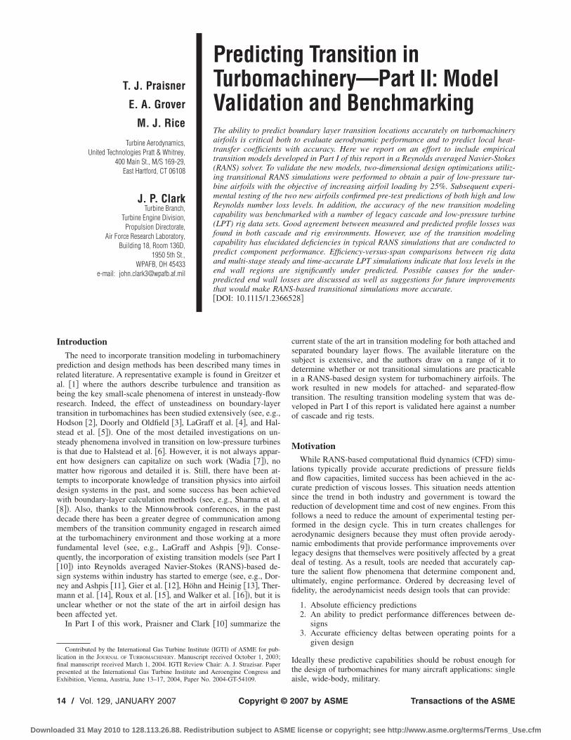
T. J. Praisner

E. A. Grover

M. J. Rice

Turbine Aerodynamics,United Technologies Pratt & Whitney,

400 Main St., M/S 169-29,East Hartford, CT 06108

J. P. ClarkTurbine Branch,

Turbine Engine Division,Propulsion Directorate,

Air Force Research Laboratory,Building 18, Room 136D,

1950 5th St.,WPAFB, OH 45433


Predicting Transition inTurbomachinery—Part II: ModelValidation and BenchmarkingThe ability to predict boundary layer transition locations accurately on turbomachineryairfoils is critical both to evaluate aerodynamic performance and to predict local heat-transfer coefficients with accuracy. Here we report on an effort to include empiricaltransition models developed in Part I of this report in a Reynolds averaged Navier-Stokes(RANS) solver. To validate the new models, two-dimensional design optimizations utiliz-ing transitional RANS simulations were performed to obtain a pair of low-pressure tur-bine airfoils with the objective of increasing airfoil loading by 25%. Subsequent experi-mental testing of the two new airfoils confirmed pre-test predictions of both high and lowReynolds number loss levels. In addition, the accuracy of the new transition modelingcapability was benchmarked with a number of legacy cascade and low-pressure turbine(LPT) rig data sets. Good agreement between measured and predicted profile losses wasfound in both cascade and rig environments. However, use of the transition modelingcapability has elucidated deficiencies in typical RANS simulations that are conducted topredict component performance. Efficiency-versus-span comparisons between rig dataand multi-stage steady and time-accurate LPT simulations indicate that loss levels in theend wall regions are significantly under predicted. Possible causes for the under-predicted end wall losses are discussed as well as suggestions for future improvementsthat would make RANS-based transitional simulations more accurate.�DOI: 10.1115/1.2366528�

IntroductionThe need to incorporate transition modeling in turbomachinery

prediction and design methods has been described many times inrelated literature. A representative example is found in Greitzer etal. �1� where the authors describe turbulence and transition asbeing the key small-scale phenomena of interest in unsteady-flowresearch. Indeed, the effect of unsteadiness on boundary-layertransition in turbomachines has been studied extensively �see, e.g.,Hodson �2�, Doorly and Oldfield �3�, LaGraff et al. �4�, and Hal-stead et al. �5��. One of the most detailed investigations on un-steady phenomena involved in transition on low-pressure turbinesis that due to Halstead et al. �6�. However, it is not always appar-ent how designers can capitalize on such work �Wadia �7��, nomatter how rigorous and detailed it is. Still, there have been at-tempts to incorporate knowledge of transition physics into airfoildesign systems in the past, and some success has been achievedwith boundary-layer calculation methods �see, e.g., Sharma et al.�8��. Also, thanks to the Minnowbrook conferences, in the pastdecade there has been a greater degree of communication amongmembers of the transition community engaged in research aimedat the turbomachinery environment and those working at a morefundamental level �see, e.g., LaGraff and Ashpis �9��. Conse-quently, the incorporation of existing transition models �see Part I�10�� into Reynolds averaged Navier-Stokes �RANS�-based de-sign systems within industry has started to emerge �see, e.g., Dor-ney and Ashpis �11�, Gier et al. �12�, Höhn and Heinig �13�, Ther-mann et al. �14�, Roux et al. �15�, and Walker et al. �16��, but it isunclear whether or not the state of the art in airfoil design hasbeen affected yet.

In Part I of this work, Praisner and Clark �10� summarize the

current state of the art in transition modeling for both attached andseparated boundary layer flows. The available literature on thesubject is extensive, and the authors draw on a range of it todetermine whether or not transitional simulations are practicablein a RANS-based design system for turbomachinery airfoils. Thework resulted in new models for attached- and separated-flowtransition. The resulting transition modeling system that was de-veloped in Part I of this report is validated here against a numberof cascade and rig tests.

MotivationWhile RANS-based computational fluid dynamics �CFD� simu-

lations typically provide accurate predictions of pressure fieldsand flow capacities, limited success has been achieved in the ac-curate prediction of viscous losses. This situation needs attentionsince the trend in both industry and government is toward thereduction of development time and cost of new engines. From thisfollows a need to reduce the amount of experimental testing per-formed in the design cycle. This in turn creates challenges foraerodynamic designers because they must often provide aerody-namic embodiments that provide performance improvements overlegacy designs that themselves were positively affected by a greatdeal of testing. As a result, tools are needed that accurately cap-ture the salient flow phenomena that determine component and,ultimately, engine performance. Ordered by decreasing level offidelity, the aerodynamicist needs design tools that can provide:

1. Absolute efficiency predictions2. An ability to predict performance differences between de-

signs3. Accurate efficiency deltas between operating points for a

given design

Ideally these predictive capabilities should be robust enough forthe design of turbomachines for many aircraft applications: singleaisle, wide-body, military.

Contributed by the International Gas Turbine Institute �IGTI� of ASME for pub-lication in the JOURNAL OF TURBOMACHINERY. Manuscript received October 1, 2003;final manuscript received March 1, 2004. IGTI Review Chair: A. J. Strazisar. Paperpresented at the International Gas Turbine Institute and Aeroengine Congress andExhibition, Vienna, Austria, June 13–17, 2004, Paper No. 2004-GT-54109.

14 / Vol. 129, JANUARY 2007 Copyright © 2007 by ASME Transactions of the ASME


Figure 1�a� is a plot of measured-versus-predicted efficiencylevels for five low-pressure turbines �LPTs�. The predicted valueswere obtained from fully turbulent steady CFD simulations runwith ideal �i.e., smooth� end walls. First, the absolute levels ofefficiency can not be accurately predicted with fully turbulentCFD simulations as executed here, as evidenced by the fact thatonly one of the five predictions falls on the “exact-match” line.Second, the ranking of the five designs from the CFD results is fardifferent than the actual �measured� ranking. So, the fully turbu-lent simulations executed for this effort also do not predict perfor-mance differences, even qualitatively, between designs. Finally,the measured and predicted results for a LPT at takeoff and cruiseReynolds numbers are shown in Fig. 1�b� While the absolute ef-ficiency is well predicted by the turbulent simulation for the take-off condition, the cruise efficiency level is significantly over pre-dicted. The results in Fig. 1�b� indicated that turbulent CFDsimulations of LPTs are also not able to predict efficiency deltasbetween design points for a given design. So, fully turbulent CFDis not capable of fulfilling any of the aerodynamicist’s three re-quirements for an effective design tool as regards the LPT.

It is believed that inaccuracies in efficiency predictions ob-tained from fully turbulent, steady RANS simulations are a con-sequence of an inability to predict accurately:

1. Non wall-bounded shear flows which include:

1.1. Mixing of flow distortions/wakes1.2. Losses associated with end wall/secondary flows1.3. Effects of cavity and main-gas-path interactions

2. Unsteady effects3. The transitional nature of attached and separated airfoil

boundary layers.

The goal of this study is to develop a tool that can accuratelymodel the transitional nature of airfoil boundary layers in axial-flow turbomachinery. However, some attention will be paid tounsteady effects and non-wall bounded shear flows, and an efforthas been made to elucidate other RANS modeling issues throughthe systematic validation of the transition-prediction capability.

This validation/benchmarking effort focuses on LPT airfoils be-cause the high aspect ratios that typify these airfoils can allow forthe clear discrimination of profile loss levels from other lossmechanisms. Additionally, LPT airfoils display the full multi-moded �Mayle �17�� nature of turbomachinery-related transition,and an inability to predict attached- and separated-flow transitionin the LPT can mean the difference between success and failure ofthe design.

Particular attention will be paid to the prediction of loss andefficiency levels in this report as they are the primary quantities ofconcern to the aerodynamic designer. Only a fraction of thebenchmarking cases executed for validation and benchmarking of

the modeling capability are presented here. The cases that arepresented were chosen to demonstrate the systematic approach ofthe validation effort. Benchmarking with profile-loss data fromhigh aspect ratio cascades is presented first, and this is followedby comparisons between predicted and measured spanwise lossdata from cascades. Next, results from validation studies withspanwise efficiency data from multi-stage LPT rigs are presented.Finally, comparisons are made between measured and predictedlevels of integrated and mid-span efficiency levels for engines andrigs.

Computational MethodsSteady-state and time-resolved turbine flowfields were pre-

dicted using the three-dimensional �3D� RANS code describedcollectively by Ni �18�, Ni and Bogoian �19�, and Davis et al.�20�. Numerical closure for turbulent flow is obtained via thek-� turbulence model as described by Wilcox �21�. An O-H gridtopology was employed with approximately 40,000 grid pointsper passage for two-dimensional �2D� simulations and approxi-mately 600,000 grid points per passage for three-dimensionalsimulations without tip clearance. These grid counts provided es-sentially grid-independent solutions with values of y+ of the order1 and approximately 7 grid points per momentum thickness. Insteady mode the code is accurate to second order in space, multi-grid techniques are used to obtain rapid convergence, and amixing-plane model is employed at each inter-row boundary. Toaccount for losses generated by the mixing of flow distortions, theexit flow field from each row is circumferentially “mixed out” bya control-volume analysis that assumes a constant-area conditionfor the mixing process. The resulting one-dimensional span-wiseprofiles are then passed into the downstream row.

When run in time-accurate mode, the code employs implicitdual time stepping to solve for the periodic, unsteady flow field,and a sliding grid interface exists at inter-row boundaries. Thecode is accurate to second order in space and time, and multi-gridtechniques are used for the inner subiterations. For the time-accurate LPT rig simulations, up to 27 million grid points, distrib-uted across 102 CPUs, were needed per simulation. Finally, freestream values of k and � were set for each validation case accord-ing to the methods outlined in Praisner and Clark �10� �i.e., Part I�.

The attached- and separated-flow transition models developedin Praisner and Clark �10� were incorporated into the solver with-out any additional modifications or tuning to data beyond theirdevelopment. As stated in Praisner and Clark �10�, predicted tran-sition locations were handled as abrupt trips in the code. Extrapo-lation outside of the development space of each model is allowedin the code. However, if extrapolation occurs in a simulation,detailed feedback is output to the user indicating the dimension-less parameters that were outside the bounds of the database usedto build the correlation.

Attention was paid to postprocess the predicted flow fields con-sistently with the data reduction techniques used for each bench-mark data set. The boundary conditions used for each simulationare described in detail below, as warranted. For simplicity, endwall flows were treated as fully turbulent for all computationalresults presented. As mentioned in Part I of this report, no mod-eling for roughness effects on pre-transitional laminar boundarylayers exists in the current transition-prediction system. Conse-quently, only validation cases for which aerodynamically smoothsurface conditions existed are presented.

Steady 2D Validation ResultsFigure 2 is a plot of measured and predicted convective heat

load distributions around the high-pressure turbine inlet guidevane of Arts et al. �22�. Results are shown from CFD simulationswith fully turbulent, fully laminar, and transitional modeling ofthe boundary layers on the airfoil. Note that modeling of the ef-fects of free stream turbulence on the pre-transitional boundarylayers �Praisner and Clark �10�� was employed for the transitional

Fig. 1 Measured-versus-predicted efficiencies for five LPTs attakeoff conditions „a…, and for an LPT at takeoff and cruise con-ditions „b…



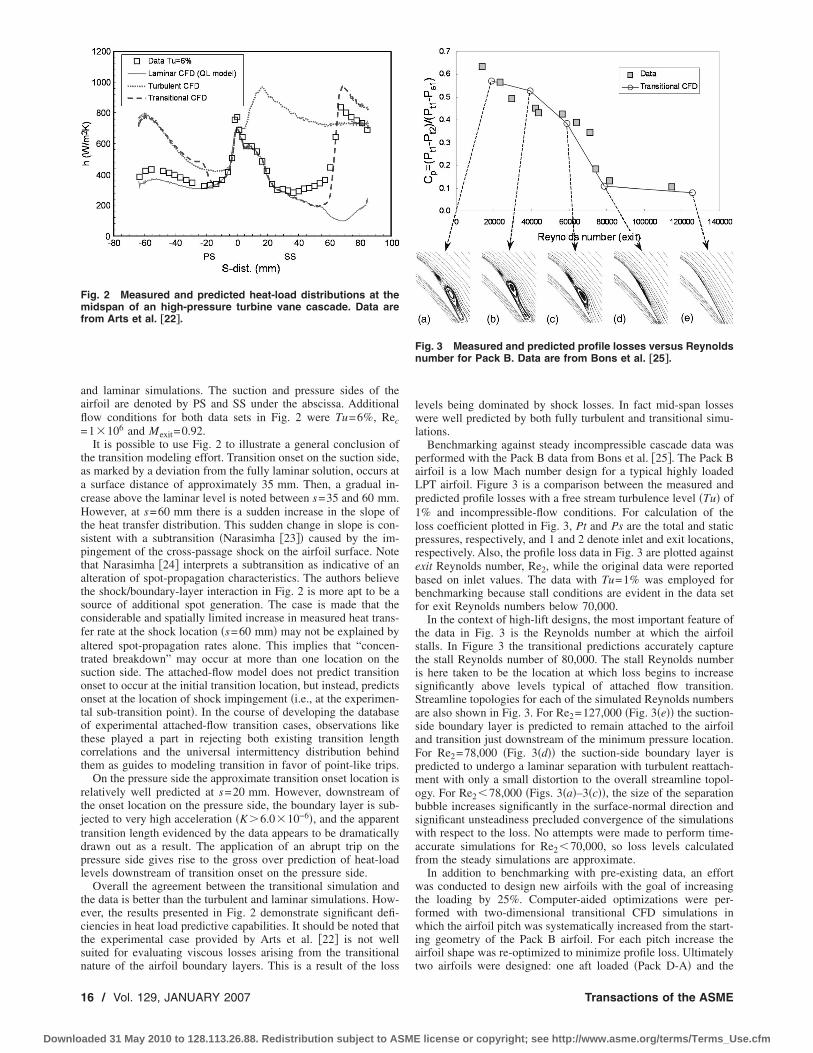
and laminar simulations. The suction and pressure sides of theairfoil are denoted by PS and SS under the abscissa. Additionalflow conditions for both data sets in Fig. 2 were Tu=6%, Rec=1�106 and Mexit=0.92.

It is possible to use Fig. 2 to illustrate a general conclusion ofthe transition modeling effort. Transition onset on the suction side,as marked by a deviation from the fully laminar solution, occurs ata surface distance of approximately 35 mm. Then, a gradual in-crease above the laminar level is noted between s=35 and 60 mm.However, at s=60 mm there is a sudden increase in the slope ofthe heat transfer distribution. This sudden change in slope is con-sistent with a subtransition �Narasimha �23�� caused by the im-pingement of the cross-passage shock on the airfoil surface. Notethat Narasimha �24� interprets a subtransition as indicative of analteration of spot-propagation characteristics. The authors believethe shock/boundary-layer interaction in Fig. 2 is more apt to be asource of additional spot generation. The case is made that theconsiderable and spatially limited increase in measured heat trans-fer rate at the shock location �s=60 mm� may not be explained byaltered spot-propagation rates alone. This implies that “concen-trated breakdown” may occur at more than one location on thesuction side. The attached-flow model does not predict transitiononset to occur at the initial transition location, but instead, predictsonset at the location of shock impingement �i.e., at the experimen-tal sub-transition point�. In the course of developing the databaseof experimental attached-flow transition cases, observations likethese played a part in rejecting both existing transition lengthcorrelations and the universal intermittency distribution behindthem as guides to modeling transition in favor of point-like trips.

On the pressure side the approximate transition onset location isrelatively well predicted at s=20 mm. However, downstream ofthe onset location on the pressure side, the boundary layer is sub-jected to very high acceleration �K�6.0�10−6�, and the apparenttransition length evidenced by the data appears to be dramaticallydrawn out as a result. The application of an abrupt trip on thepressure side gives rise to the gross over prediction of heat-loadlevels downstream of transition onset on the pressure side.

Overall the agreement between the transitional simulation andthe data is better than the turbulent and laminar simulations. How-ever, the results presented in Fig. 2 demonstrate significant defi-ciencies in heat load predictive capabilities. It should be noted thatthe experimental case provided by Arts et al. �22� is not wellsuited for evaluating viscous losses arising from the transitionalnature of the airfoil boundary layers. This is a result of the loss

levels being dominated by shock losses. In fact mid-span losseswere well predicted by both fully turbulent and transitional simu-lations.

Benchmarking against steady incompressible cascade data wasperformed with the Pack B data from Bons et al. �25�. The Pack Bairfoil is a low Mach number design for a typical highly loadedLPT airfoil. Figure 3 is a comparison between the measured andpredicted profile losses with a free stream turbulence level �Tu� of1% and incompressible-flow conditions. For calculation of theloss coefficient plotted in Fig. 3, Pt and Ps are the total and staticpressures, respectively, and 1 and 2 denote inlet and exit locations,respectively. Also, the profile loss data in Fig. 3 are plotted againstexit Reynolds number, Re2, while the original data were reportedbased on inlet values. The data with Tu=1% was employed forbenchmarking because stall conditions are evident in the data setfor exit Reynolds numbers below 70,000.

In the context of high-lift designs, the most important feature ofthe data in Fig. 3 is the Reynolds number at which the airfoilstalls. In Figure 3 the transitional predictions accurately capturethe stall Reynolds number of 80,000. The stall Reynolds numberis here taken to be the location at which loss begins to increasesignificantly above levels typical of attached flow transition.Streamline topologies for each of the simulated Reynolds numbersare also shown in Fig. 3. For Re2=127,000 �Fig. 3�e�� the suction-side boundary layer is predicted to remain attached to the airfoiland transition just downstream of the minimum pressure location.For Re2=78,000 �Fig. 3�d�� the suction-side boundary layer ispredicted to undergo a laminar separation with turbulent reattach-ment with only a small distortion to the overall streamline topol-ogy. For Re2�78,000 �Figs. 3�a�–3�c��, the size of the separationbubble increases significantly in the surface-normal direction andsignificant unsteadiness precluded convergence of the simulationswith respect to the loss. No attempts were made to perform time-accurate simulations for Re2�70,000, so loss levels calculatedfrom the steady simulations are approximate.

In addition to benchmarking with pre-existing data, an effortwas conducted to design new airfoils with the goal of increasingthe loading by 25%. Computer-aided optimizations were per-formed with two-dimensional transitional CFD simulations inwhich the airfoil pitch was systematically increased from the start-ing geometry of the Pack B airfoil. For each pitch increase theairfoil shape was re-optimized to minimize profile loss. Ultimatelytwo airfoils were designed: one aft loaded �Pack D-A� and the

Fig. 2 Measured and predicted heat-load distributions at themidspan of an high-pressure turbine vane cascade. Data arefrom Arts et al. †22‡.

Fig. 3 Measured and predicted profile losses versus Reynoldsnumber for Pack B. Data are from Bons et al. †25‡.



other front loaded �Pack D-F�. An exit Reynolds number of128,000, which is typical of cruise conditions, was held for thedesigns of the Pack D airfoils. A Zweifel load coefficient of 1.40was achieved with both Pack D designs. For reference the Pack Bhas a Zweifel load coefficient of approximately 1.15, where theload coefficient is defined as:

CL = 2�

bxsin2 �2�Cx1

Cx2cot �1 + cot �2� �1�

In Eq. �1�, � is the pitch, bx is the axial chord, �1 and �2 are theinlet and exit flow angles, and Cx1 and Cx2 are the inlet and exitaxial velocities, respectively. Both the Pack D-A and D-F airfoilsviolated standard design practices at Pratt & Whitney for LPTdesigns. In addition, no airfoils were present in the database ofcases used to develop the two transition models with CL�1.2.Finally, it was not necessary to use extrapolation of the transitionmodels beyond their development space in the design of the PackD airfoils

Low Mach number testing �M �3� of the Pack D geometrieswas conducted with a passive-grid generated free stream turbu-lence level of 2% at an engine-specific turbulence length scale ofapproximately 10% of axial chord. Profile loss-versus-Reynolds-number data and transitional CFD predictions are shown in Fig. 4for the Pack D-A airfoil. The data depicted in this figure are fromSjolander �26� and the computational results presented were per-

formed before the experimental data were recorded �i.e., they aretrue pre-test predictions�. As indicated by the loss data, the PackD-A airfoil has a stall Reynolds number of approximately 120,000for the free stream conditions considered. Transitional simulationsaccurately predict the stall Reynolds number for the Pack D-Aairfoil in that the airfoil experienced non-reattaching separationsfor Re2�120,000. Loss levels for Reynolds numbers higher thanthe stall Reynolds number are also well predicted. The significantunder prediction of losses for Reynolds numbers below 120,000 isrelated to the fact that a steady solution could not be obtainedonce stall occurred. Also, the streamline topology shown in Fig. 4for the lowest Reynolds number indicates that the separation inthe stalled condition for this high-lift, aft-loaded design is moredramatic than that of the lower lift, mid-loaded Pack B design. Asin the Pack-B validation study, time-accurate simulations were notrun for Reynolds numbers below the stall value.

Also shown in Fig. 4 is the loss data for the Pack D-F airfoilwith the same free stream conditions as those held for the PackD-A testing. For the Reynolds numbers and free stream conditionsconsidered in testing, the Pack D-F airfoil did not experience stall.The predicted loss levels are within the experimental uncertainty,for all Reynolds numbers for this airfoil. Additionally, the losslevels of the Pack D-F airfoil matched, with experimental uncer-tainty, those of the base line, Pack B design at all Reynolds num-bers for the same flow conditions. The Pack B data are not shownin Fig. 4 for clarity. So, in addition to predicting the stall Reynoldsnumber accurately for the Pack D-A design, the transition model-ing capability predicted the performance benefits of a front-loadeddesign.

Figure 5 is a plot of measured and predicted static-pressuredistributions for the aft region of the Pack D-F airfoil at Re2=56,000 and the Pack D-A airfoil at Re2=160,000. The localvariation in the pressure distributions caused by laminar separa-tions on both airfoils is evident in the data. These separation-related features in the static-pressure distributions are reasonablywell captured by the transition modeling system. As the computa-tional separation bubbles for both cases are very thin in the wallnormal dimension, no streamline images were included in Fig. 5.

The results of the 2D steady validation effort show that, forsystematic reductions in Reynolds number, the interplay of theattached- and separated-flow transition models captures loss-versus-Reynolds-number behavior for the test cases considered. Inother words, the attached-flow model predicts transition in a man-ner that results in the formation of a laminar separation at theappropriate Reynolds number. Following the formation of a lami-

Fig. 4 Measured and predicted profile losses plotted versusexit Reynolds number for the Pack D-A and Pack D-F airfoils

Fig. 5 Measured and predicted pressure loadings for the aft region of „a… thePack D-F airfoil at Re2=56,000 and „b… the Pack D-A airfoil at Re2=160,000. Dataare from Sjolander †26‡.



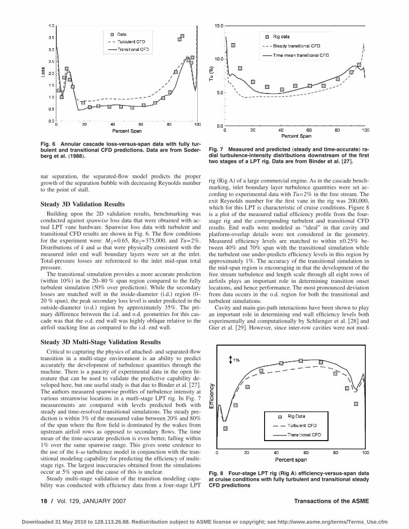
nar separation, the separated-flow model predicts the propergrowth of the separation bubble with decreasing Reynolds numberto the point of stall.

Steady 3D Validation ResultsBuilding upon the 2D validation results, benchmarking was

conducted against spanwise loss data that were obtained with ac-tual LPT vane hardware. Spanwise loss data with turbulent andtransitional CFD results are shown in Fig. 6. The flow conditionsfor the experiment were: M2=0.65, Re2=375,000, and Tu=2%.Distributions of k and � that were physically consistent with themeasured inlet end wall boundary layers were set at the inlet.Total-pressure losses are referenced to the inlet mid-span totalpressure.

The transitional simulation provides a more accurate prediction�within 10%� in the 20–80 % span region compared to the fullyturbulent simulation �50% over prediction�. While the secondarylosses are matched well in the inside-diameter �i.d.� region �0–20 % span�, the peak secondary loss level is under predicted in theoutside-diameter �o.d.� region by approximately 35%. The pri-mary difference between the i.d. and o.d. geometries for this cas-cade was that the o.d. end wall was highly oblique relative to theairfoil stacking line as compared to the i.d. end wall.

Steady 3D Multi-Stage Validation ResultsCritical to capturing the physics of attached- and separated-flow

transition in a multi-stage environment is an ability to predictaccurately the development of turbulence quantities through themachine. There is a paucity of experimental data in the open lit-erature that can be used to validate the predictive capability de-veloped here, but one useful study is that due to Binder et al. �27�.The authors measured spanwise profiles of turbulence intensity atvarious streamwise locations in a mutli-stage LPT rig. In Fig. 7measurements are compared with levels predicted both withsteady and time-resolved transitional simulations. The steady pre-diction is within 3% of the measured value between 20% and 80%of the span where the flow field is dominated by the wakes fromupstream airfoil rows as opposed to secondary flows. The timemean of the time-accurate prediction is even better, falling within1% over the same spanwise range. This gives some credence tothe use of the k-� turbulence model in conjunction with the tran-sitional modeling capability for predicting the efficiency of multi-stage rigs. The largest inaccuracies obtained from the simulationsoccur at 5% span and the cause of this is unclear.

Steady multi-stage validation of the transition modeling capa-bility was conducted with efficiency data from a four-stage LPT

rig �Rig A� of a large commercial engine. As in the cascade bench-marking, inlet boundary layer turbulence quantities were set ac-cording to experimental data with Tu=2% in the free stream. Theexit Reynolds number for the first vane in the rig was 200,000,which for this LPT is characteristic of cruise conditions. Figure 8is a plot of the measured radial efficiency profile from the four-stage rig and the corresponding turbulent and transitional CFDresults. End walls were modeled as “ideal” in that cavity andplatform-overlap details were not considered in the geometry.Measured efficiency levels are matched to within ±0.25% be-tween 40% and 70% span with the transitional simulation whilethe turbulent one under-predicts efficiency levels in this region byapproximately 1%. The accuracy of the transitional simulation inthe mid-span region is encouraging in that the development of thefree stream turbulence and length scale through all eight rows ofairfoils plays an important role in determining transition onsetlocations, and hence performance. The most pronounced deviationfrom data occurs in the o.d. region for both the transitional andturbulent simulations.

Cavity and main-gas-path interactions have been shown to playan important role in determining end wall efficiency levels bothexperimentally and computationally by Schlienger et al. �28� andGier et al. �29�. However, since inter-row cavities were not mod-

Fig. 6 Annular cascade loss-versus-span data with fully tur-bulent and transitional CFD predictions. Data are from Soder-berg et al. „1988….

Fig. 7 Measured and predicted „steady and time-accurate… ra-dial turbulence-intensity distributions downstream of the firsttwo stages of a LPT rig. Data are from Binder et al. †27‡.

Fig. 8 Four-stage LPT rig „Rig A… efficiency-versus-span dataat cruise conditions with fully turbulent and transitional steadyCFD predictions



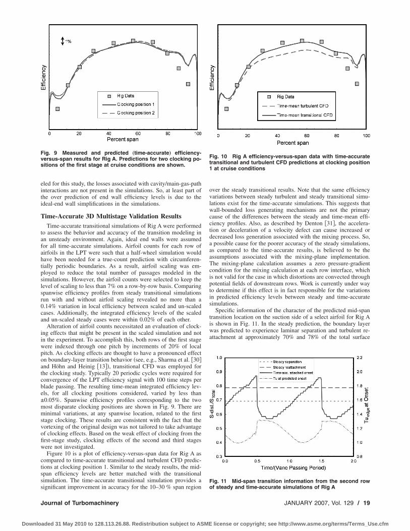
eled for this study, the losses associated with cavity/main-gas-pathinteractions are not present in the simulations. So, at least part ofthe over prediction of end wall efficiency levels is due to theideal-end wall simplifications in the simulations.

Time-Accurate 3D Multistage Validation ResultsTime-accurate transitional simulations of Rig A were performed

to assess the behavior and accuracy of the transition modeling inan unsteady environment. Again, ideal end walls were assumedfor all time-accurate simulations. Airfoil counts for each row ofairfoils in the LPT were such that a half-wheel simulation wouldhave been needed for a true-count prediction with circumferen-tially periodic boundaries. As a result, airfoil scaling was em-ployed to reduce the total number of passages modeled in thesimulations. However, the airfoil counts were selected to keep thelevel of scaling to less than 7% on a row-by-row basis. Comparingspanwise efficiency profiles from steady transitional simulationsrun with and without airfoil scaling revealed no more than a0.14% variation in local efficiency between scaled and un-scaledcases. Additionally, the integrated efficiency levels of the scaledand un-scaled steady cases were within 0.02% of each other.

Alteration of airfoil counts necessitated an evaluation of clock-ing effects that might be present in the scaled simulation and notin the experiment. To accomplish this, both rows of the first stagewere indexed through one pitch by increments of 20% of localpitch. As clocking effects are thought to have a pronounced effecton boundary-layer transition behavior �see, e.g., Sharma et al. �30�and Höhn and Heinig �13��, transitional CFD was employed forthe clocking study. Typically 20 periodic cycles were required forconvergence of the LPT efficiency signal with 100 time steps perblade passing. The resulting time-mean integrated efficiency lev-els, for all clocking positions considered, varied by less than±0.05%. Spanwise efficiency profiles corresponding to the twomost disparate clocking positions are shown in Fig. 9. There areminimal variations, at any spanwise location, related to the firststage clocking. These results are consistent with the fact that thevortexing of the original design was not tailored to take advantageof clocking effects. Based on the weak effect of clocking from thefirst-stage study, clocking effects of the second and third stageswere not investigated.

Figure 10 is a plot of efficiency-versus-span data for Rig A ascompared to time-accurate transitional and turbulent CFD predic-tions at clocking position 1. Similar to the steady results, the mid-span efficiency levels are better matched with the transitionalsimulation. The time-accurate transitional simulation provides asignificant improvement in accuracy for the 10–30 % span region

over the steady transitional results. Note that the same efficiencyvariations between steady turbulent and steady transitional simu-lations exist for the time-accurate simulations. This suggests thatwall-bounded loss generating mechanisms are not the primarycause of the differences between the steady and time-mean effi-ciency profiles. Also, as described by Denton �31�, the accelera-tion or deceleration of a velocity defect can cause increased ordecreased loss generation associated with the mixing process. So,a possible cause for the poorer accuracy of the steady simulations,as compared to the time-accurate results, is believed to be theassumptions associated with the mixing-plane implementation.The mixing-plane calculation assumes a zero pressure-gradientcondition for the mixing calculation at each row interface, whichis not valid for the case in which distortions are convected throughpotential fields of downstream rows. Work is currently under wayto determine if this effect is in fact responsible for the variationsin predicted efficiency levels between steady and time-accuratesimulations.

Specific information of the character of the predicted mid-spantransition location on the suction side of a select airfoil for Rig Ais shown in Fig. 11. In the steady prediction, the boundary layerwas predicted to experience laminar separation and turbulent re-attachment at approximately 70% and 78% of the total surface

Fig. 9 Measured and predicted „time-accurate… efficiency-versus-span results for Rig A. Predictions for two clocking po-sitions of the first stage at cruise conditions are shown.

Fig. 10 Rig A efficiency-versus-span data with time-accuratetransitional and turbulent CFD predictions at clocking position1 at cruise conditions

Fig. 11 Mid-span transition information from the second rowof steady and time-accurate simulations of Rig A



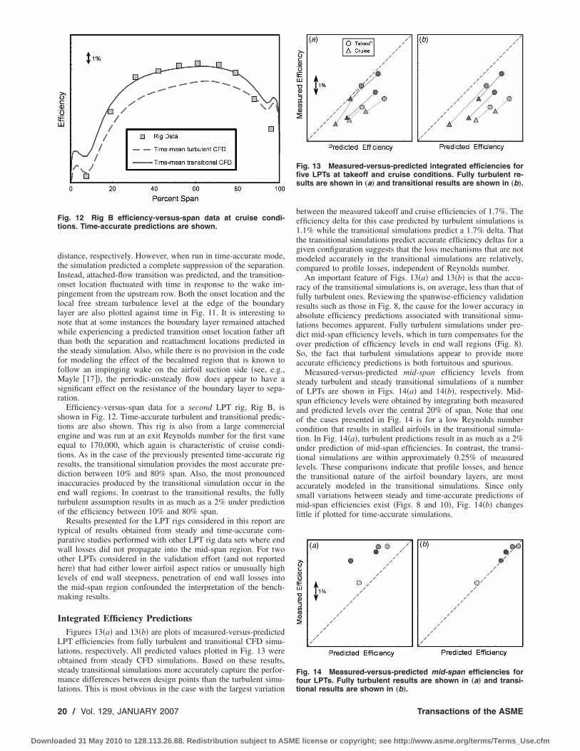
distance, respectively. However, when run in time-accurate mode,the simulation predicted a complete suppression of the separation.Instead, attached-flow transition was predicted, and the transition-onset location fluctuated with time in response to the wake im-pingement from the upstream row. Both the onset location and thelocal free stream turbulence level at the edge of the boundarylayer are also plotted against time in Fig. 11. It is interesting tonote that at some instances the boundary layer remained attachedwhile experiencing a predicted transition onset location father aftthan both the separation and reattachment locations predicted inthe steady simulation. Also, while there is no provision in the codefor modeling the effect of the becalmed region that is known tofollow an impinging wake on the airfoil suction side �see, e.g.,Mayle �17��, the periodic-unsteady flow does appear to have asignificant effect on the resistance of the boundary layer to sepa-ration.

Efficiency-versus-span data for a second LPT rig, Rig B, isshown in Fig. 12. Time-accurate turbulent and transitional predic-tions are also shown. This rig is also from a large commercialengine and was run at an exit Reynolds number for the first vaneequal to 170,000, which again is characteristic of cruise condi-tions. As in the case of the previously presented time-accurate rigresults, the transitional simulation provides the most accurate pre-diction between 10% and 80% span. Also, the most pronouncedinaccuracies produced by the transitional simulation occur in theend wall regions. In contrast to the transitional results, the fullyturbulent assumption results in as much as a 2% under predictionof the efficiency between 10% and 80% span.

Results presented for the LPT rigs considered in this report aretypical of results obtained from steady and time-accurate com-parative studies performed with other LPT rig data sets where endwall losses did not propagate into the mid-span region. For twoother LPTs considered in the validation effort �and not reportedhere� that had either lower airfoil aspect ratios or unusually highlevels of end wall steepness, penetration of end wall losses intothe mid-span region confounded the interpretation of the bench-making results.

Integrated Efficiency PredictionsFigures 13�a� and 13�b� are plots of measured-versus-predicted

LPT efficiencies from fully turbulent and transitional CFD simu-lations, respectively. All predicted values plotted in Fig. 13 wereobtained from steady CFD simulations. Based on these results,steady transitional simulations more accurately capture the perfor-mance differences between design points than the turbulent simu-lations. This is most obvious in the case with the largest variation

between the measured takeoff and cruise efficiencies of 1.7%. Theefficiency delta for this case predicted by turbulent simulations is1.1% while the transitional simulations predict a 1.7% delta. Thatthe transitional simulations predict accurate efficiency deltas for agiven configuration suggests that the loss mechanisms that are notmodeled accurately in the transitional simulations are relatively,compared to profile losses, independent of Reynolds number.

An important feature of Figs. 13�a� and 13�b� is that the accu-racy of the transitional simulations is, on average, less than that offully turbulent ones. Reviewing the spanwise-efficiency validationresults such as those in Fig. 8, the cause for the lower accuracy inabsolute efficiency predictions associated with transitional simu-lations becomes apparent. Fully turbulent simulations under pre-dict mid-span efficiency levels, which in turn compensates for theover prediction of efficiency levels in end wall regions �Fig. 8�.So, the fact that turbulent simulations appear to provide moreaccurate efficiency predictions is both fortuitous and spurious.

Measured-versus-predicted mid-span efficiency levels fromsteady turbulent and steady transitional simulations of a numberof LPTs are shown in Figs. 14�a� and 14�b�, respectively. Mid-span efficiency levels were obtained by integrating both measuredand predicted levels over the central 20% of span. Note that oneof the cases presented in Fig. 14 is for a low Reynolds numbercondition that results in stalled airfoils in the transitional simula-tion. In Fig. 14�a�, turbulent predictions result in as much as a 2%under prediction of mid-span efficiencies. In contrast, the transi-tional simulations are within approximately 0.25% of measuredlevels. These comparisons indicate that profile losses, and hencethe transitional nature of the airfoil boundary layers, are mostaccurately modeled in the transitional simulations. Since onlysmall variations between steady and time-accurate predictions ofmid-span efficiencies exist �Figs. 8 and 10�, Fig. 14�b� changeslittle if plotted for time-accurate simulations.

Fig. 12 Rig B efficiency-versus-span data at cruise condi-tions. Time-accurate predictions are shown.

Fig. 13 Measured-versus-predicted integrated efficiencies forfive LPTs at takeoff and cruise conditions. Fully turbulent re-sults are shown in „a… and transitional results are shown in „b….

Fig. 14 Measured-versus-predicted mid-span efficiencies forfour LPTs. Fully turbulent results are shown in „a… and transi-tional results are shown in „b….



Spanwise-integrated steady efficiency predictions of a limitednumber of the LPTs are compared to measured levels in Fig. 15�a�while time-accurate results for the same LPTs are shown in Fig.15�b�. The efficiency over predictions for time-accurate simula-tions are, on average, approximately half those from steady tran-sitional simulations. These results are consistent with the compari-sons made between steady and time-accurate spanwise efficiencyresults for the four-stage LPT rig presented in the preceding sec-tion.

It was shown in previous sections of this paper that secondaryloss predictions from the CFD simulations can be inaccurate forannular cascade data, particularly in the o.d. region �e.g., see Fig.6.�. Since secondary losses are generally known to be independentof Reynolds number, it is believed that the inability of the RANSsimulations presented here to capture accurately the end walllosses, contributes to the inaccurate absolute efficiency predic-tions. An additional cause for the poor absolute predictions isbelieved to be the simplified geometric modeling of the end walls.However, the primary cause for over-predicted efficiency levelsfrom steady simulations �as presented here� may be attributable toassumptions made in the inter-row mixing-plane implementation.This was demonstrated in the significant reductions in efficiencyover predictions between steady and time-accurate simulations�Fig. 15�.

ConclusionsThree levels of fidelity that might be provided by RANS simu-

lations for efficiency predictions of turbomachinery componentsare: �1� absolute efficiency levels, �2� performance differences be-tween designs, and �3� efficiency deltas between operating pointsfor a given design. The goal of this work was to model the tran-sitional nature of boundary layers on turbomachinery airfoils inRANS simulations to determine if efficiency-prediction improve-ments could be realized in any of the aforementioned categories.Attached- and separated-flow transition models, developed in PartI of this paper, were incorporated into a RANS-based system forairfoil design, and a validation and benchmarking study was con-ducted.

The transition models were implemented here using point-wisetrips with no transition length modeling or use of the universalintermittency distribution. The models provided a significant im-provement in the accuracy of predicted profile losses for bothcascades and multi-stage LPT rigs over the fully turbulent as-sumption. Validation against cascade data also demonstrated thatthe new modeling capability accurately captures the interplay be-tween the physics of attached- and separated-flow transitionmodes for the test cases considered. To further demonstrate themodeling capabilities, two low-pressure turbine airfoils were de-signed that had Zweifel load coefficients of 1.4 �a 25% increaseover the base line level�. The stall Reynolds numbers of both

airfoils were accurately predicted with the transition-modeling ca-pability in advance of testing. Further, one design �i.e., the front-loaded one� was resistant to stall for exit Reynolds numbers below50,000 while also matching the performance level of the base linedesign. So, by incorporating modeling of the physics of transitioninto the design system at an adequate level, it was demonstratedthat the design space for LPT airfoils was significantly extended.

More accurate predictions of profile losses were demonstratedboth for airfoils that experienced attached-flow transition �wherefully turbulent RANS over predicts loss� and for those that expe-rienced separated-flow transition �where fully turbulent RANS un-der predicts loss�. However, considering the relative merits of theattached- and separated-flow models, it appears that the former ismore effective than the latter. This is not surprising since, as seenin Part I of this work �10�, the attached-flow model is grounded inthe basic physics of bypass transition, while the separated-flowmodel is more of a straightforward correlation of variables. Con-sequently, the authors believe that future work should focus onmodeling separated flow transition. In addition, a modeling capa-bility that captures the effects of surface roughness on pre-transitional boundary layers is needed.

It was found that the addition of transition modeling to thedesign system proved effective for determining efficiency deltasbetween design points and profile losses for individual low-pressure turbines. No improvements were realized concerning theaccuracy of predicted absolute levels of efficiency and the abilityto predict efficiency deltas between engine designs. However, theability to predict mid-span performance allows one to infer muchabout secondary-flow and cavity/main-gas-path interaction lossmechanisms and the ability of RANS simulations, employing two-equation turbulence models and ideal end walls, to capture themproperly. This means that, particularly for low-aspect-ratio com-ponents, further work is necessary in the pursuit of accurate pre-dictions of secondary-flows and cavity/main-gas-path interactions.

AcknowledgmentThe authors would like to thank Pratt & Whitney for granting

permission to publish this work. In particular, they are grateful toDr. Jayant Sabnis, Gary Stetson, and Joel Wagner for their sup-port. Inspiration for this work is a result of the authors’ participa-tion in the Minnowbrook conferences that are sponsored by theU.S. Air Force Office of Scientific Research and NASA �see, e.g.,NASA CP 1998-206958�. Professor T. V. Jones and Professor JimS.-J. Chen taught the authors the importance of starting any tech-nical effort from basic principles, and additional insights weregleaned from discussions with A. A. Rangwalla, M. F. Blair, F.Ames, T. Fukuda, O. P. Sharma, S. S. Magge, D. Zhang, G. Barter,and J. Dailey.

References�1� Greitzer, E. M., Tan, C. S., Wisler, D. C., Adamczyk, J. J., and Strazisar, A. J.,

1994, “Unsteady Flows in Turbomachines: Where’s the Beef?” UnsteadyFlows in Aeropropulsion, ASME AD-40, New York, pp. 1–11.

�2� Hodson, H. P., 1984, “Boundary Layer and Loss Measurements on the Rotorof an Axial-Flow Turbine,” ASME J. Eng. Gas Turbines Power, 106, pp.391–399.

�3� Doorly, D. J., and Oldfield, M. L. G., 1985, “Simulation of Wake Passing in aStationary Turbine Rotor Cascade,” AIAA J. Propulsion, Vol. 1�4�, pp. 316–318.

�4� LaGraff, J. E., Ashworth, D. A., and Schultz, D. L., 1989, “Measurement andModeling of the Gas Turbine Blade Transition Process as Disturbed byWakes,” ASME J. Turbomach., 111, pp. 315–322.

�5� Halstead, D. E., Wisler, D. C., Okiishi, T. H., Walker, G. J., Hodson, H. P., andShin, H. W., 1997, “Boundary Layer Development in Axial Compressors andTurbines: Part 1 of 4—Composite Picture,” ASME J. Turbomach., 119, pp.114–126.

�6� Halstead, D. E., Wisler, D. C., Okiishi, T. H., Walker, G. J., Hodson, H. P., andShin, H. W., 1997, “Boundary Layer Development in Axial Compressors andTurbines: Part 3 of 4—LP Turbines,” ASME J. Turbomach., 119, pp. 225–237.

�7� Wadia, A., 2003, personal communication.�8� Sharma, O. P., Wells, R. A., Schlinker, R. H., and Bailey, D. A., 1982,

“Boundary Layer Development on Airfoil Suction Surfaces,” ASME J. Eng.Power, 104, pp. 698–706.

Fig. 15 Measured-versus-predicted integrated efficiencies forthree LPTs. Steady transitional results are shown in „a… andtime-accurate transitional results are shown in „b….



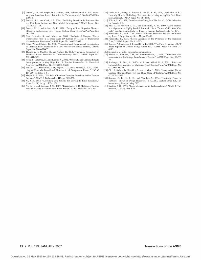
�9� LaGraff, J. E., and Ashpis, D. E., editors, 1998, “Minnowbrook II: 1997 Work-shop on Boundary Layer Transition in Turbomachines,” NASA/CP-1998–206958.

�10� Praisner, T. J., and Clark, J. P., 2004, “Predicting Transition in Turbomachin-ery, Part I—A Review and New Model Development,” ASME Report No.GT-2004–54108.

�11� Dorney, D. J., and Ashpis, D. E., 1998, “Study of Low Reynolds NumberEffects on the Losses in Low-Pressure Turbine Blade Rows,” AIAA Paper No.98–3575.

�12� Gier, J., Ardey, S., and Heisler, A., 2000, “Analysis of Complex Three-Dimensional Flow in a Three-Stage LP Turbine by Means of TransitionalNavier-Stokes Simulation,” ASME Paper No. 2000GT-645.

�13� Höhn, W., and Heinig, K., 2000, “Numerical and Experimental Investigationof Unsteady Flow Interaction in a Low Pressure Multistage Turbine,” ASMEPaper No. 2000-GT-437.

�14� Thermann, H., Mueller, M., and Niehuis, R., 2001, “Numerical Simulation ofBoundary Layer Transition in Turbomachinery Flows,” ASME Paper No.2001-GT-0475.

�15� Roux, J., Lefebvre, M., and Liamis, N., 2002, “Unsteady and Calming EffectsInvestigation on a Very High Lift LP Turbine Blade—Part II: NumericalAnalysis,” ASME Paper No. GT-2002–30228.

�16� Walker, G. J., Henderson, A. D., Hughes, J. D., and Coupland, J., 2003, “Mod-eling of Unsteady Transitional Flow on Axial Compressor Blades,” NASA/TM-2004-212913, p. 57.

�17� Mayle, R. E., 1991, “The Role of Laminar Turbulent Transition in Gas TurbineEngines,” ASME J. Turbomach., 113, pp. 509–537.

�18� Ni, R. H., 1982, “A Multiple-Grid Scheme for Solving the Euler Equations,”AIAA J., 20�11�, pp. 1565–1571.

�19� Ni, R. H., and Bogoian, J. C., 1989, “Prediction of 3-D Multistage TurbineFlowfield Using a Multiple-Grid Euler Solver,” AIAA Paper No. 89–0203.

�20� Davis, R. L., Shang, T., Buteau, J., and Ni, R. H., 1996, “Prediction of 3-DUnsteady Flow in Multi-Stage Turbomachinery Using an Implicit Dual Time-Step Approach,” AIAA Paper No. 96–2565.

�21� Wilcox, D. C., 1998, Turbulence Modeling for CFD, 2nd ed., DCW Industries,La Canada, CA.

�22� Arts, T., de Rouvroit, L. M., and Rutherford, A. W., 1990, “Aero-ThermalInvestigation of a Highly Loaded Transonic Linear Turbine Guide Vane Cas-cade,” von Karman Institute for Fluids Dynamics Technical Note No. 174.

�23� Narasimha, R., 1985, “The Laminar Turbulent Transition Zone in the Bound-ary Layer,” Prog. Aerosp. Sci., 22, pp. 29–80.

�24� Narasimha, R., 1991, “Recent Advances in the Dynamics of the TransitionZone,” ISABE Report No. 91–7006.

�25� Bons, J. P., Sondergaard, R., and Rivir, R., 2001, “The Fluid Dynamics of LPTBlade Separation Control Using Pulsed Jets,” ASME Paper No. 2001-GT-0190.

�26� Sjolander, S., 2003, personal communication.�27� Binder, A., Schröder, T. H., and Hourmouziadis, J., 1988, “Turbulence Mea-

surements in a Multistage Low-Pressure Turbine,” ASME Paper No. 88-GT-79.

�28� Schlienger, J., Pfau, A., Kalfas, A. I., and Abhari, R. S., 2003, “Effects ofLabyrinth Seal Variation on Multistage Axial Turbine Flow,” ASME Paper No.GT-2003–38270.

�29� Gier, J., Stubert, B., Brouillet, B., and de Vito, L., 2003, “Interaction of ShroudLeakage Flow and Main Flow in a Three-Stage LP Turbine,” ASME Paper No.GT2003–38025.

�30� Sharma, O. P., Ni, R. H., and Tanrikut, S., 1994, “Unsteady Flows inTurbines—Impact on Design Procedure,” in AGARD Lecture Series 195, Tur-bomachinery Design Using CFD.

�31� Denton, J. D., 1993, “Loss Mechanisms in Turbomachines,” ASME J. Tur-bomach., 115, pp. 621–656.



W. Colban

K. A. Thole

Mechanical Engineering Department,Virginia Tech,

Blacksburg, VA

M. HaendlerSiemens Power Generation,

Muelheim a. d. Ruhr, Germany

Experimental and ComputationalComparisons of Fan-ShapedFilm Cooling on a Turbine VaneSurfaceThe flow exiting the combustor in a gas turbine engine is considerably hotter than themelting temperature of the turbine section components, of which the turbine nozzle guidevanes see the hottest gas temperatures. One method used to cool the vanes is to use rowsof film-cooling holes to inject bleed air that is lower in temperature through an array ofdiscrete holes onto the vane surface. The purpose of this study was to evaluate therow-by-row interaction of fan-shaped holes as compared to the performance of a singlerow of fan-shaped holes in the same locations. This study presents adiabatic film-coolingeffectiveness measurements from a scaled-up, two-passage vane cascade. High-resolutionfilm-cooling measurements were made with an infrared camera at a number of enginerepresentative flow conditions. Computational fluid dynamics predictions were also madeto evaluate the performance of some of the current turbulence models in predicting acomplex flow such as turbine film-cooling. The renormalization group (RNG) k-� turbu-lence model gave a closer prediction of the overall level of film effectiveness, while thev2-f turbulence model gave a more accurate representation of the flow physics seen in theexperiments. �DOI: 10.1115/1.2370747�

IntroductionThe nozzle guide vanes in a gas turbine, located directly down-

stream of the combustion section, are particularly susceptible tothermal failure, with gas temperatures commonly reaching levelsabove component latent melting temperatures. Combustion tem-peratures continue to rise in an effort to increase the efficiency andpower output from gas turbine engines. This rise has led to theincreased demand to devise better cooling schemes and more re-silient materials from which to manufacture the turbine vanes.Many cooling strategies are typically used at the same time, in-cluding impingement cooling, internal passage cooling, and exter-nal film cooling. Although designing various cooling configura-tions, consideration must also be given to the structural integrityof the vanes, since turbine vanes are under extremely high thermalstresses.

Ideally, film cooling aims to inject cooler temperature fluid overthe surface of the vane, shielding it from the high-temperaturefreestream gases. This goal is sometimes difficult to achieve, how-ever, as the nature of the flow through the turbine passage tends tobe uncompromising with conditions, including high freestreamturbulence, secondary flows, high surface curvature, rapid flowacceleration, and high-pressure gradients, all of which have beenshown to affect cooling performance. Film cooling offers the en-gine designer an enticing way to extend part life; however, the useof too much coolant flow from the compressor takes a toll on theoverall engine efficiency. To counteract this consequence, enginedesigners are constantly on the lookout for ways to maintain oreven increase the cooling performance but with less coolant.

Alternative hole geometries are sometimes used by engine de-signers, such as the diffused or so-called fan-shaped holes, tomaximize the performance of the injected coolant. By expandingthe exit of the cooling hole in the lateral direction, the effectivemomentum of the surface coolant can be reduced prior to injec-

tion. Goldstein et al. �1� showed that fan-shaped holes providebetter surface attachment at higher blowing ratios, as well as bet-ter lateral spreading of the coolant than cylindrical holes. A slightdeviation of this design is the laidback fan-shaped hole, wherein aforward expansion is also included, further inhibiting jet liftoff.The major drawback for noncylindrical hole geometries is in-creased initial manufacturing costs. The benefits, however, of fan-shaped holes are many, including increased part life �fewer re-placements needed�, less required coolant �increased engineefficiency�, and fewer holes needed �increased structural stabilityof the vane�.

Computational fluid dynamics �CFD� is becoming an essentialdesign tool in the gas turbine industry because it is both cheaperand faster than performing experiments. However, in order to relyon CFD results, it is first necessary to validate the predictions withmeasurements to ensure computational reliability. In this study,detailed comparisons of the measured adiabatic effectiveness dataare made to CFD predictions using both the renormalization group�RNG� k-� and v2-f turbulence models.

The standard k-� turbulence model is a Reynolds-averagedNavier-Stokes �RANS� model with two transport equations—onefor the turbulent kinetic energy �k� and one for the eddy viscosity��—which are used to approximate the turbulent viscosity ��t�.The RNG k-� model involves renormalization group theory andadds a term to the eddy viscosity transport equation, which makesthe model better for high strain flows than the standard k-� model.One major drawback of the RNG k-� model in wall-boundedflows, such as film cooling, is the assumption of isotropic turbu-lence. The existence of the wall introduces anisotropy in the nor-mal fluctuations, the presence of which are not accounted for inthe wall functions used to approximate the behavior in the bound-ary layer in the k-� turbulence models. Wall functions lose theirreliability in three-dimensions or separated flow regimes, such assometimes seen in film cooling.

Durbin �2� incorporated turbulence anisotropy in the near wallregion into the existing k-� RANS model by adding two transportequations—one for the normal fluctuations �v2� and one for anelliptic relaxation function �f�—and effectively removed the ne-

Contributed by the Turbomachinery Division of ASME for publication in theJOURNAL OF TURBOMACHINERY. Manuscript received January 12, 2006; final manu-script received January 29, 2006. Review conducted by D. Wisler.



cessity of wall functions. The v2-f turbulence model correctlymodels the blocking phenomenon near the wall that is responsiblefor attenuating the normal turbulent fluctuations, eliminating therequirement of damping functions in wall bounded flows.

Film-cooling effectiveness has been predicted using both theRNG k-� and the v2-f turbulence models in our paper. The com-plete passage, including the contoured end wall was modeled inthe RNG k-� simulation for a baseline case. A spanwise periodicsection of the vane passage was modeled using the v2-f turbulencemodel for the same blowing ratios that were measured experimen-tally.

This study is the first to present detailed high-resolution adia-batic film-cooling effectiveness measurements for a turbine vanewith multiple rows of fan-shaped film-cooling holes at enginerepresentative blowing ratios. Contours and laterally averaged val-ues of adiabatic film-cooling effectiveness are presented for boththe pressure and suction sides. Adiabatic film-cooling effective-ness data are critical information for engine designers, necessaryto predict not only metal temperatures but also to validate CFDpredictions.

Past StudiesBecause of its crucial role in preventing thermal failure in gas

turbine engines, film cooling has been an extensively researchedtopic over the last 30–35 years �3,4�. Flat-plate studies have en-compassed a variation of every possible geometrical parameter,including surface angle, entrance length, hole spacing, compoundangle, lateral expansion angle, forward expansion angle, area ra-tio, and multiple row configurations. External conditions have alsobeen thoroughly investigated for flat plates, including such effectsas turbulence intensity, pressure gradient, and the state of the ap-proaching boundary layer. An excellent review of the relevantshaped hole literature, which primarily focused on flat-plate stud-ies, was given by Bunker �5�. Although flat plate studies are a keyfirst step in understanding the flow physics for a given coolinghole geometry, to completely understand the flow physics andevaluate a given film-cooling design, it must be tested on theactual turbine vane. It stands to reason that the flow physics on ahighly curved surface, such as a turbine vane, coupled with mul-tiple cooling row interaction, could yield results that are differentfrom the flat-plate special case. Some studies have presented re-sults for partially and/or fully cooled nozzle guide vanes, but thedeficiency of many of those studies is the lack of high-resolutioneffectiveness measurements.

Studies involving a single row of fan-shaped cooling holes on avane surface have been performed by Zhang et al. �6�, Zhang andPudupatty �7�, and Colban et al. �8�. Using the same experimentalprocedure and facilities for both studies, effectiveness measure-ments were made with fan-shaped holes on the suction side byZhang et al. �6� and on the pressure side by Zhang and Pudupatty�7�. Results indicated an increase in effectiveness on the suctionside for the blowing ratio range from 0.5 to 1.5 and a decrease ineffectiveness on the pressure side for the blowing ratio range from1.5 to 2.5.

Colban et al. �8� presented adiabatic effectiveness measure-ments for eight single rows of fan-shaped holes on both the pres-sure and suction sides in the same facilities as this paper. Theirresults indicated that in regions of high convex curvature, particu-larly on the suction side near the leading edge, jet liftoff wasprevalent and increased with blowing ratio. Colban et al. �8� alsonoted a decrease in effectiveness with increased blowing on thepressure side, which was attributed to partial jet liftoff and hot gasentrainment.

Despite the knowledge gained by studying single-row coolingon the vane, it is still necessary to study multiple-row film coolingon the vane. Goldstein et al. �9� showed that on a flat plate, asingle row of cooling holes separated with increasing blowingratio, resulting in decreased film effectiveness. However, with adouble-row cooling configuration, the upstream row provided the

impetus for the downstream row to stay attached to the surface.This resulted in an increased film effectiveness with blowing ratio.The study by Goldstein et al. �9� suggested that an accurate studyof vane film cooling would not be complete unless all of theengine-present film-cooling rows were tested together.

Effectiveness measurements were made by Guo et al. �10� in atransonic facility for a turbine airfoil with multiple rows of fan-shaped holes. Results showed higher values of effectiveness forfan-shaped holes than for cylindrical holes. However, the decay ineffectiveness on the pressure side was faster for fan-shaped thanfor cylindrical holes, which was most likely the result of a betterlateral coverage for the fan-shaped holes. Sargison et al. �11� alsomeasured effectiveness in an annular turbine cascade with mul-tiple rows of cylindrical, fan-shaped, and converging slot holes.They reported similar levels of performance for the fan-shapedand converging slot holes, both of which had superior perfor-mance than cylindrical holes.

Effectiveness measurements on the pressure side were made forthree rows of fan-shaped holes and isothermal showerhead blow-ing by Schnieder et al. �12�. They reported that the presence ofisothermal showerhead blowing caused increased mixing of thefirst pressure side row, lowering effectiveness. However, withshowerhead cooling, perhaps the increased mixing of the firstpressure side row might actually improve effectiveness. Polankaet al. �13� also studied the effect of showerhead blowing on thefirst downstream pressure side row, using cylindrical instead offan-shaped holes. They reported that showerhead blowing causedthe jets to stay attached, where they would normally separatewithout upstream blowing. Polanka et al. �13� suggested that in-creased turbulent mixing caused by the showerhead dispersed thejet toward the wall, reducing liftoff.

Colban et al. �8� presented effectiveness for fan-shaped holescombined with upstream showerhead blowing. Their results indi-cated that upstream showerhead blowing increased jet dispersiontoward the vane surface for the first row of film-cooling holesdownstream on the pressure side, a result consistent with the re-sults of Polanka et al. �13�. Although Colban et al. �8� presented acomplete set of high-resolution data for single-row fan-shapedholes on a turbine vane, it is further necessary to understand therow-to-row interaction, as the state of the approaching boundarylayer has been shown to have a significant effect on the perfor-mance of a film-cooling jet �14�.

There have been a limited number of computational studiesinvolving shaped hole film cooling on a flat plate. Kohli and Thole�15� used the standard k-� model with nonequilibrium wall func-tions to show the importance of modeling the interior plenumconditions correctly. A similar flat-plate study was performed byHyams and Leylek �16�, who investigated the effect of hole ge-ometry on the thermal and flow field using the high Reynoldsnumber k-� model with generalized wall functions. They showedthat laterally diffused shaped holes had the highest adiabatic ef-fectiveness levels downstream of the hole exit location.

Computational film-cooling studies on a turbine vane surfacewith fan-shaped holes have been done by Hildebrandt et al. �17�,Ferguson et al. �18�, and Heidmann et al. �19�. Only Heidmann etal. �19�, however, modeled more than one row of holes on thevane. Their study used the k-� model to simulate a periodic sec-tion of the vane with six staggered rows of cylindrical showerheadholes, four rows of fan-shaped holes on the pressure side, and tworows of cylindrical holes on the suction side. The numerical re-sults presented by Heidmann et al. �19� were not validated withexperiments; thus, the validity of the method was not established.The single-row numerical results of Ferguson et al. �18� showedgood agreement with experimental results for blowing ratios of�1.5 using the RNG k-� model with a two-layer wall treatment.Above a blowing ratio of 1.5, the agreement was not so good.

Nothing, to the author’s knowledge, as of yet has been pub-lished applying the v2-f turbulence model to film-cooling flowapplications. However, because the v2-f model is valid all the way



to the wall, with no need for wall functions or damping models inthe viscous sublayer, it stands to reason that it should be expectedto perform at least as good as the existing two-equation models ifnot better. The v2-f model has been used with success in modelingthree-dimensional turbulent boundary layers �20� as well as sepa-rated flow conditions, such as the backward-facing step and vortexshedding flows �21�.

Of the previous fan-shaped film-cooling studies that have beenperformed on a vane, the obvious deficiency is for high-resolutiondata for the fully cooled situation. This study offers the first com-pletely cooled turbine vane study with fan shaped film coolinggiving detailed experimental adiabatic film cooling effectivenessresults. Similarly, past computational studies of film cooling havebeen limited in their scope.

Experimental FacilitiesThe experiments were performed in the VTExCCL large-scale,

low-speed, recirculating wind tunnel facility shown in Fig. 1. Thisfacility was identical to the one used by Colban et al. �8� and wasdescribed in detail by that study. The main features of the facilitywere a flow split section that divided the flow into two channels,one that was heated to by a 55 kW heater bank and used as themainstream combustor exit flow and the other that was cooledusing a 40 kW chiller in series with a heat exchanger and used ascoolant flow.

The test section was a linear, two-passage cascade with a con-toured upper end wall. The inlet freestream turbulence intensitywas measured to be 1.2% a distance of 0.2 C upstream of the vaneleading edge with a hot wire anemometer. Typical mainstreamtemperature was 60°C, with a nominal difference between themainstream and coolant of 20°C, yielding a density ratio of 1.06.The pressure at the test section inlet was nearly atmospheric. A listof pertinent geometrical parameters for the test section is given inTable 1, along with certain relevant inlet conditions.

Test Section Design. To match the engine static pressure dis-tribution around the vane to that found in the engine, a contouredsurface was implemented for the upper end wall. The contouredend wall, which contracted to roughly 54% of the inlet spanheight, is shown schematically and graphically in Fig. 2. A de-tailed account of the contour design was given by Colban et al.

�8�. The contoured end wall resulted in an excellent match of theexperimental static pressure distribution at the midspan to that ofthe engine. Also, since this investigation was not focused on anythree-dimensional effects of the contour on the vane cooling, arigorous investigation, including CFD predictions and experimen-tal examination, was used to verify the presence of a two-dimensional flow regime in the area where the measurementswere taken. All of the film-cooling effectiveness measurementswere made between 5% and 32% span, while the flow was essen-tially two-dimensional below 40% span.

A schematic of the vane test section is shown in Fig. 3. Bleedvalves were used to ensure flow periodicity between the two pas-sages, and the flexible wall was used to make minor adjustmentsto the flow distribution around the center vane. Also shown in Fig.3 are the plenum locations relative to the holes, as well as the holedesignations, to be used throughout the rest of the report.

A detailed discussion of the vane design and construction wasgiven by Colban et al. �8�. The vane contained four interior ple-nums, which allowed for flow-rate control among the rows ofholes to obtain the desired blowing ratio distribution. Coolant wassupplied to the plenums from the upper channel in the wind tunnelusing the blower shown in Fig. 1. Discharge coefficients, whichwere presented in the study of Colban et al. �8�, were used to setthe combined flow rates through each plenum based on the desiredblowing ratios.

The test vane contained showerhead cooling with five in-linerows, four fan-shaped pressure side rows, and four fan-shapedsuction side rows of film-cooling holes. The diameter of the cy-lindrical inlet section of the fan-shaped holes was 0.38±0.015 cm.The diameters of each hole were measured to verify that the cor-rect flow area was used to determine the total mass flow rate andindividual blowing ratios because of slight manufacturing varia-

Fig. 1 Schematic of the low-speed recirculating wind tunnelfacility

Table 1 Operating conditions and vane parameters

Scale 3X

C �m� 0.53Smax,PS �m� 0.52Smax,SS �m� 0.68Uinlet �m/s� 10Reinlet �-� 3.0�105

�TFC �°C� 20Vane pitch �m� 0.465

Fig. 2 Contoured end-wall surface definition

Fig. 3 Schematic of experimental test section



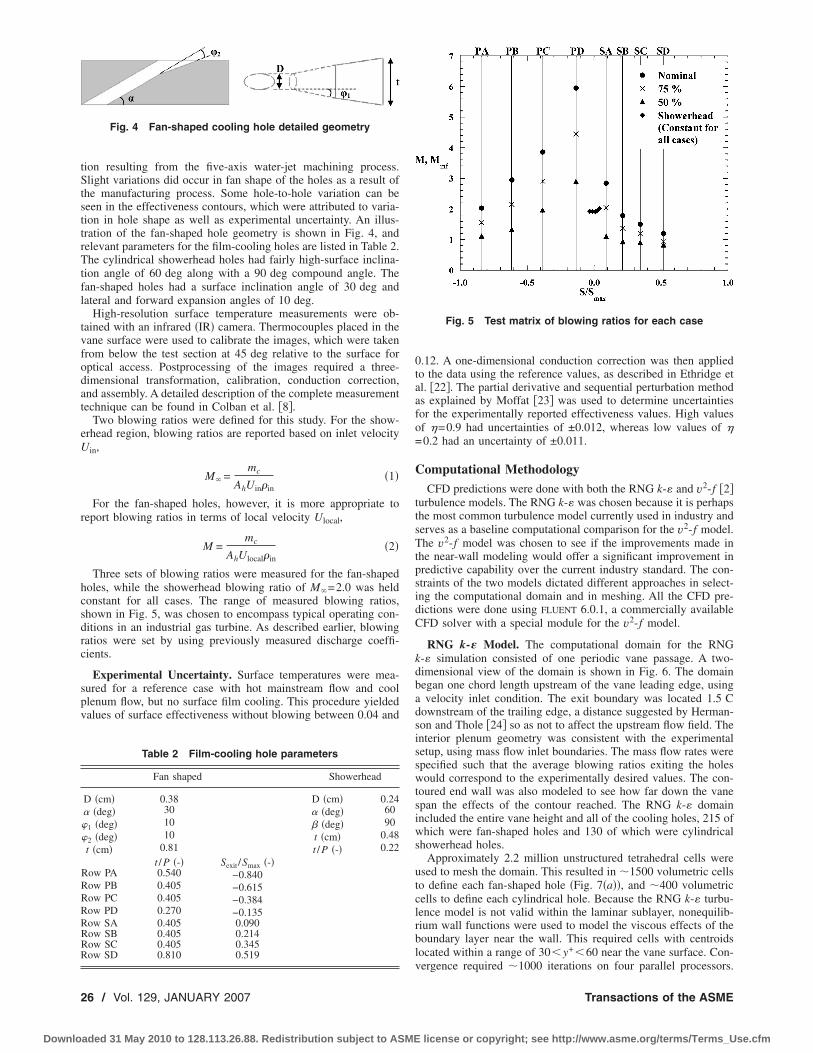
tion resulting from the five-axis water-jet machining process.Slight variations did occur in fan shape of the holes as a result ofthe manufacturing process. Some hole-to-hole variation can beseen in the effectiveness contours, which were attributed to varia-tion in hole shape as well as experimental uncertainty. An illus-tration of the fan-shaped hole geometry is shown in Fig. 4, andrelevant parameters for the film-cooling holes are listed in Table 2.The cylindrical showerhead holes had fairly high-surface inclina-tion angle of 60 deg along with a 90 deg compound angle. Thefan-shaped holes had a surface inclination angle of 30 deg andlateral and forward expansion angles of 10 deg.

High-resolution surface temperature measurements were ob-tained with an infrared �IR� camera. Thermocouples placed in thevane surface were used to calibrate the images, which were takenfrom below the test section at 45 deg relative to the surface foroptical access. Postprocessing of the images required a three-dimensional transformation, calibration, conduction correction,and assembly. A detailed description of the complete measurementtechnique can be found in Colban et al. �8�.

Two blowing ratios were defined for this study. For the show-erhead region, blowing ratios are reported based on inlet velocityUin,

M� =mc

AhUin�in�1�

For the fan-shaped holes, however, it is more appropriate toreport blowing ratios in terms of local velocity Ulocal,

M =mc

AhUlocal�in�2�

Three sets of blowing ratios were measured for the fan-shapedholes, while the showerhead blowing ratio of M�=2.0 was heldconstant for all cases. The range of measured blowing ratios,shown in Fig. 5, was chosen to encompass typical operating con-ditions in an industrial gas turbine. As described earlier, blowingratios were set by using previously measured discharge coeffi-cients.

Experimental Uncertainty. Surface temperatures were mea-sured for a reference case with hot mainstream flow and coolplenum flow, but no surface film cooling. This procedure yieldedvalues of surface effectiveness without blowing between 0.04 and

0.12. A one-dimensional conduction correction was then appliedto the data using the reference values, as described in Ethridge etal. �22�. The partial derivative and sequential perturbation methodas explained by Moffat �23� was used to determine uncertaintiesfor the experimentally reported effectiveness values. High valuesof �=0.9 had uncertainties of ±0.012, whereas low values of �=0.2 had an uncertainty of ±0.011.

Computational MethodologyCFD predictions were done with both the RNG k-� and v2-f �2�

turbulence models. The RNG k-� was chosen because it is perhapsthe most common turbulence model currently used in industry andserves as a baseline computational comparison for the v2-f model.The v2-f model was chosen to see if the improvements made inthe near-wall modeling would offer a significant improvement inpredictive capability over the current industry standard. The con-straints of the two models dictated different approaches in select-ing the computational domain and in meshing. All the CFD pre-dictions were done using FLUENT 6.0.1, a commercially availableCFD solver with a special module for the v2-f model.

RNG k-� Model. The computational domain for the RNGk-� simulation consisted of one periodic vane passage. A two-dimensional view of the domain is shown in Fig. 6. The domainbegan one chord length upstream of the vane leading edge, usinga velocity inlet condition. The exit boundary was located 1.5 Cdownstream of the trailing edge, a distance suggested by Herman-son and Thole �24� so as not to affect the upstream flow field. Theinterior plenum geometry was consistent with the experimentalsetup, using mass flow inlet boundaries. The mass flow rates werespecified such that the average blowing ratios exiting the holeswould correspond to the experimentally desired values. The con-toured end wall was also modeled to see how far down the vanespan the effects of the contour reached. The RNG k-� domainincluded the entire vane height and all of the cooling holes, 215 ofwhich were fan-shaped holes and 130 of which were cylindricalshowerhead holes.

Approximately 2.2 million unstructured tetrahedral cells wereused to mesh the domain. This resulted in �1500 volumetric cellsto define each fan-shaped hole �Fig. 7�a��, and �400 volumetriccells to define each cylindrical hole. Because the RNG k-� turbu-lence model is not valid within the laminar sublayer, nonequilib-rium wall functions were used to model the viscous effects of theboundary layer near the wall. This required cells with centroidslocated within a range of 30�y+�60 near the vane surface. Con-vergence required �1000 iterations on four parallel processors.

Fig. 4 Fan-shaped cooling hole detailed geometry

Table 2 Film-cooling hole parameters

Fan shaped Showerhead

D �cm� 0.38 D �cm� 0.24 �deg� 30 �deg� 601 �deg� 10 � �deg� 902 �deg� 10 t �cm� 0.48t �cm� 0.81 t / P �-� 0.22

t / P �-� Sexit /Smax �-�Row PA 0.540 −0.840Row PB 0.405 −0.615Row PC 0.405 −0.384Row PD 0.270 −0.135Row SA 0.405 0.090Row SB 0.405 0.214Row SC 0.405 0.345Row SD 0.810 0.519

Fig. 5 Test matrix of blowing ratios for each case



The simulations took approximately two days to converge. Con-vergence was determined not only from residuals, but also bymonitoring area-averaged surface temperatures on both the suc-tion and pressure sides. The drag coefficient around the vane wasalso monitored as a check on aerodynamic convergence. A gridindependence study was also performed by adapting the grid up to3.9 million cells, but no significant change in results was observedso the initial grid size of 2.2 millions cells was deemed sufficient.

v2-f Model. Unlike the RNG k-� model, the v2-f model is validto the wall. This required a structured grid in the vicinity of thewall, resolving the boundary layer to within y+�3. Consequently,modeling the entire span was not a possibility for the v2-f modeldue to the higher cell density required near the wall. For this

reason, only a 6 cm spanwise periodic section was included in thecomputational domain, which is shown schematically in Fig. 6.Both the experimental results and the RNG k-� CFD resultsshowed periodicity below the midspan; thus, it was valid to modelonly the small periodic section, thus making the computationsfeasible.

The v2-f model grid contained �1.6 million cells in order toget the near-wall resolution. The vane surface was meshed with anunstructured grid, and a boundary layer mesh was applied to thevane surface �shown in Fig. 7�b��. Consequently, there were pris-matic cells to a distance of 1.5 cm from the wall, at which pointthe remainder of the domain was meshed with unstructured tetra-hedral cells. The surface mesh resolution is shown for the v2-fsimulations in Fig. 7�c�. Solutions were run for 500 iterations on afirst-order upwind scheme, before being switched over to asecond-order upwind scheme with SIMPLEC coupling for 1500 it-erations. The v2-f model computations were run on three parallelprocessors and required approximately three days to reach conver-gence. As with the RNG k-� model, the surface temperatures anddrag coefficient were monitored as additional convergence crite-ria.

ResultsPrior to performing the multiple-row adiabatic film-cooling

measurements, the experimental method and data reduction pro-cedure were validated for a single-row and compared to existingpublished data. Figure 8 shows laterally averaged single-row ef-fectiveness downstream of row SC, a row that was located in arelatively flat region of the vane. Because of differences in holegeometry and spacing, the distance downstream of the hole exitwas normalized with respect to the equivalent exit slot width s,where s was the ratio of the hole breakout area to the hole spacingP. The results show excellent agreement with the flat-plate studyby Gritsch et al. �25�, thus validating both the experimental anddata reduction methods.

Pressure Side. Adiabatic film-cooling effectiveness contoursfor each case are shown in Fig. 9 for the pressure side. In total,five images were required to completely capture the pressure side,with measurements taken in the nominally 2D flow region of thevane. The showerhead cooling was largely ineffective at coolingthe leading edge region, which Colban et al. �8� attributed to jetliftoff from the high surface angle. The first row of fan-shapedholes showed liftoff by a narrowing in the jet contour just down-stream of the hole exit. However, downstream near S /Smax=−0.20, the jets began to spread laterally. This was a result of the

Fig. 6 2D view of the CFD domain „the RNG k-� model fea-tured the entire span and contour, whereas the v2-f predictionfeatured only a 6 cm spanwise periodic section…

Fig. 7 Computational grid sample of „a… the RNG k-� surfacemesh, „b… the v2-f boundary layer mesh, and „c… the v2-f surfacemesh

Fig. 8 Comparison of results to previously published data



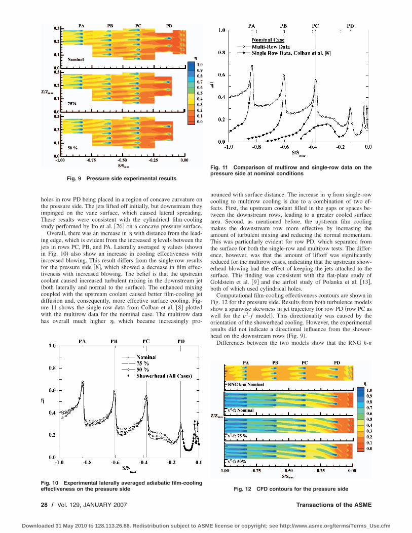
holes in row PD being placed in a region of concave curvature onthe pressure side. The jets lifted off initially, but downstream theyimpinged on the vane surface, which caused lateral spreading.These results were consistent with the cylindrical film-coolingstudy performed by Ito et al. �26� on a concave pressure surface.

Overall, there was an increase in � with distance from the lead-ing edge, which is evident from the increased � levels between thejets in rows PC, PB, and PA. Laterally averaged � values �shownin Fig. 10� also show an increase in cooling effectiveness withincreased blowing. This result differs from the single-row resultsfor the pressure side �8�, which showed a decrease in film effec-tiveness with increased blowing. The belief is that the upstreamcoolant caused increased turbulent mixing in the downstream jet�both laterally and normal to the surface�. The enhanced mixingcoupled with the upstream coolant caused better film-cooling jetdiffusion and, consequently, more effective surface cooling. Fig-ure 11 shows the single-row data from Colban et al. �8� plottedwith the multirow data for the nominal case. The multirow datahas overall much higher �, which became increasingly pro-

nounced with surface distance. The increase in � from single-rowcooling to multirow cooling is due to a combination of two ef-fects. First, the upstream coolant filled in the gaps or spaces be-tween the downstream rows, leading to a greater cooled surfacearea. Second, as mentioned before, the upstream film coolingmakes the downstream row more effective by increasing theamount of turbulent mixing and reducing the normal momentum.This was particularly evident for row PD, which separated fromthe surface for both the single-row and multirow tests. The differ-ence, however, was that the amount of liftoff was significantlyreduced for the multirow cases, indicating that the upstream show-erhead blowing had the effect of keeping the jets attached to thesurface. This finding was consistent with the flat-plate study ofGoldstein et al. �9� and the airfoil study of Polanka et al. �13�,both of which used cylindrical holes.

Computational film-cooling effectiveness contours are shown inFig. 12 for the pressure side. Results from both turbulence modelsshow a spanwise skewness in jet trajectory for row PD �row PC aswell for the v2-f model�. This directionality was caused by theorientation of the showerhead cooling. However, the experimentalresults did not indicate a directional influence from the shower-head on the downstream rows �Fig. 9�.

Differences between the two models show that the RNG k-�

Fig. 9 Pressure side experimental results

Fig. 10 Experimental laterally averaged adiabatic film-coolingeffectiveness on the pressure side

Fig. 11 Comparison of multirow and single-row data on thepressure side at nominal conditions

Fig. 12 CFD contours for the pressure side



predictions were more accurate in terms of the overall level offilm-cooling effectiveness. However, the RNG k-� predictionshowed a wider coolant footprint than the experimental results,whereas the v2-f predictions showed a much narrower coolantfootprint similar to the experimental results. Another physicaltrend shown by the v2-f that was not picked up by the RNG k-�prediction was the spreading of the coolant downstream of thefirst fan-shaped row due to liftoff and reattachment. Neither modelaccurately predicted the showerhead behavior. The RNG k-�model underpredicted the showerhead liftoff, while the v2-fmodel overpredicted the amount of liftoff in the showerheadregion.

A comparison of laterally averaged effectiveness at nominalconditions between the experimental results and both computa-tional models is shown in Fig. 13. Again, the RNG k-� modelmore accurately predicted the overall levels of �, while the v2-fmodel grossly overpredicted � on the pressure side. It is interest-ing to note that the v2-f model predicted a continual rise in effec-tiveness, indicating a buildup of coolant from upstream rows. TheRNG k-� model however, showed no row-to-row increase in ef-fectiveness, which can be seen not only in the laterally averagedvalues of Fig. 13, but in the contour of Fig. 12.

The difference in behavior between the two models in the nearleading-edge region can be seen by examining the streamlines.Streamlines for the nominal blowing conditions are shown in Fig.14 for both turbulence models. The RNG k-� model showed thestreamlines stay attached to the surface with little lateral spread-ing, whereas the v2-f model showed greater lateral spreading afteran initial jet liftoff. Also, the skewness in the jets for both modelswas illustrated by the streamlines as a compound effect from theshowerhead film cooling, which had a 90 deg compound anglewith respect to the main flow.

Suction Side. Contours of � are shown for the experimentalresults on the suction side in Fig. 15. Significant showerhead lift-off occurred, as on the pressure side, causing poor leading-edgeregion cooling. The jets on the first two suction side rows �SA andSB� separated from the surface at high blowing ratios due to thehigh curvature and acceleration in that region. Overall, � in-creased with surface distance from the stagnation line on the suc-tion side, as seen from the laterally averaged � values in Fig. 16.Near the leading edge, � decreased with blowing ratio because ofthe jet separation. However, as we progress along the suction side,the curvature decreases, and the amount of liftoff consequentlyalso decreases. This led to a reversal in trend of � with blowingrates by the end of the suction side.

The effect of multiple cooling rows as opposed to the single-row results of Colban et al. �8� for the nominal flow conditions areshown in Fig. 17. In contrast to the pressure side, where shower-head liftoff also occurred, the effect of the showerhead on the firstsuction side row was not as significant. On the suction side, theseparated showerhead coolant could not remain close enough to

Fig. 13 Pressure-side comparison of laterally averaged filmeffectiveness with computations

Fig. 14 Streamlines near the leading edge for „a… RNG k-� and„b… v2-f models at nominal conditions

Fig. 15 Experimental results on the suction side

Fig. 16 Experimental laterally averaged adiabatic film-coolingeffectiveness on the suction side



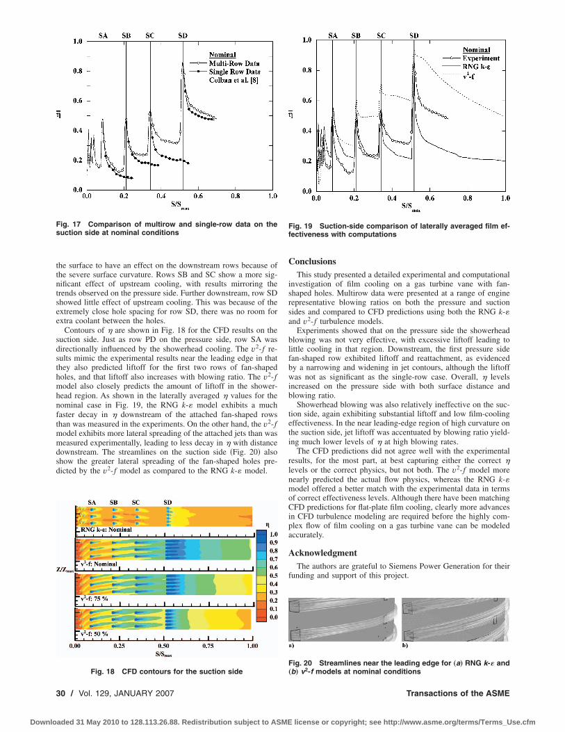
the surface to have an effect on the downstream rows because ofthe severe surface curvature. Rows SB and SC show a more sig-nificant effect of upstream cooling, with results mirroring thetrends observed on the pressure side. Further downstream, row SDshowed little effect of upstream cooling. This was because of theextremely close hole spacing for row SD, there was no room forextra coolant between the holes.

Contours of � are shown in Fig. 18 for the CFD results on thesuction side. Just as row PD on the pressure side, row SA wasdirectionally influenced by the showerhead cooling. The v2-f re-sults mimic the experimental results near the leading edge in thatthey also predicted liftoff for the first two rows of fan-shapedholes, and that liftoff also increases with blowing ratio. The v2-fmodel also closely predicts the amount of liftoff in the shower-head region. As shown in the laterally averaged � values for thenominal case in Fig. 19, the RNG k-� model exhibits a muchfaster decay in � downstream of the attached fan-shaped rowsthan was measured in the experiments. On the other hand, the v2-fmodel exhibits more lateral spreading of the attached jets than wasmeasured experimentally, leading to less decay in � with distancedownstream. The streamlines on the suction side �Fig. 20� alsoshow the greater lateral spreading of the fan-shaped holes pre-dicted by the v2-f model as compared to the RNG k-� model.

ConclusionsThis study presented a detailed experimental and computational

investigation of film cooling on a gas turbine vane with fan-shaped holes. Multirow data were presented at a range of enginerepresentative blowing ratios on both the pressure and suctionsides and compared to CFD predictions using both the RNG k-�and v2-f turbulence models.

Experiments showed that on the pressure side the showerheadblowing was not very effective, with excessive liftoff leading tolittle cooling in that region. Downstream, the first pressure sidefan-shaped row exhibited liftoff and reattachment, as evidencedby a narrowing and widening in jet contours, although the liftoffwas not as significant as the single-row case. Overall, � levelsincreased on the pressure side with both surface distance andblowing ratio.

Showerhead blowing was also relatively ineffective on the suc-tion side, again exhibiting substantial liftoff and low film-coolingeffectiveness. In the near leading-edge region of high curvature onthe suction side, jet liftoff was accentuated by blowing ratio yield-ing much lower levels of � at high blowing rates.

The CFD predictions did not agree well with the experimentalresults, for the most part, at best capturing either the correct �levels or the correct physics, but not both. The v2-f model morenearly predicted the actual flow physics, whereas the RNG k-�model offered a better match with the experimental data in termsof correct effectiveness levels. Although there have been matchingCFD predictions for flat-plate film cooling, clearly more advancesin CFD turbulence modeling are required before the highly com-plex flow of film cooling on a gas turbine vane can be modeledaccurately.

AcknowledgmentThe authors are grateful to Siemens Power Generation for their

funding and support of this project.

Fig. 17 Comparison of multirow and single-row data on thesuction side at nominal conditions

Fig. 18 CFD contours for the suction side

Fig. 19 Suction-side comparison of laterally averaged film ef-fectiveness with computations

Fig. 20 Streamlines near the leading edge for „a… RNG k-� and„b… v2-f models at nominal conditions



NomenclatureA � areaC � vane true chord

CD � discharge coefficientD � film-cooling hole diameterf � elliptic relaxation functionk � turbulent kinetic energy

kcond � thermal conductivitym � mass flow rateM � blowing ratio using local velocity,

M =mc /AhUlocal�inM� � blowing ratio using inlet velocity,

M�=mc /AhUin�inP � hole spacing measured normal to streamwise

directionP � vane pitch

Re � Reynolds number, Re=UinC / s � equivalent slot width, s=Abreak/ PS � distance along the vane surfacet � hole breakout width

T � temperatureU � velocityv2 � normal velocity fluctuationsX � distance downstream of the hole exit

y+ � wall coordinateZ � distance measured along the vane span

Greek � inclination angle� � compound angle� � eddy viscosity, surface emmissivity

�t � turbulent viscosity � kinematic viscosity� � adiabatic film-cooling effectiveness, �= �T�

−Tad� / �T�−Tc�� density

1 � lateral diffusion angle2 � forward expansion angle

Subscriptsad � adiabatic

break � hole breakout areac � coolant

exit � hole exith � metering area of film-cooling holes based on D

in � inlet conditionlocal � local conditionsmax � maximum

plenum � plenum conditionssurf � surface

� � freestream conditions

References�1� Goldstein, R. J., Eckert, E. R. G., and Burggraf, F., 1974, “Effects of Hole

Geometry and Density on Three-Dimensional Film Cooling,” Int. J. Heat MassTransfer, 17, pp. 595–607.

�2� Durbin, P. A., 1991, “Near-Wall Turbulence Closure Modeling Without‘Damping Functions’,” Theor. Comput. Fluid Dyn., 3, pp. 1–13.

�3� Kercher, D. M., 2003, Film-Cooling Bibliography: 1940–2002: private publi-cation.

�4� Kercher, D. M., 2005, Film-Cooling Bibliography Addendum: 1999–2004, pri-vate publication.

�5� Bunker, R. S., 2005, “A Review of Shaped Hole Turbine Film-Cooling Tech-nology,” ASME J. Heat Transfer, 127, pp. 441–453.

�6� Zhang, L., Baltz, M., Pudupatty, R., and Fox, M., 1999, “Turbine NozzleFilm-Cooling Study Using the Pressure Sensitive Paint �PSP� Technique,”ASME Paper No. 99-GT-196.

�7� Zhang, L., and Pudupatty, R., 2000, “The Effects of Injection Angle and HoleExit Shape on Turbine Nozzle Pressure Side Film-Cooling,” ASME Paper No.2000-GT-247.

�8� Colban, W., Gratton, A., Thole, K. A., and Haendler, M., 2006, “Heat Transferand Film-Cooling Measurements on a Stator Vane With Fan-Shaped CoolingHoles,” ASME J. Turbomach., 128, pp. 53–61.

�9� Goldstein, R. J., Eckert, E. R. G., Chiang, H. D., and Elovic, E., 1985, “Effectof Surface Roughness on Film Cooling Performance,” ASME J. Eng. GasTurbines Power, 107, pp. 111–116.

�10� Guo, S. M., Lai, C. C., Jones, T. V., Oldfield, M. L. G., Lock, G. D., andRawlinson, A. J., 1998, “The Application of Thin-Film Technology to MeasureTurbine-Vane Heat Transfer and Effectiveness in a Film-Cooled, Engine-Simulated Environment,” Int. J. Heat Fluid Flow, 19, pp. 594–600.

�11� Sargison, J. E., Guo, S. M., Oldfield, M. L. G., Lock, G. D., and Rawlinson, A.J., 2001, “A Converging Slot-Hole Film-Cooling Geometry—Part II: Tran-sonic Nozzle Guide Vane Heat Transfer and Loss,” ASME Paper No. 2001-GT-0127.

�12� Schnieder, M., Parneix, S., and von Wolfersdorf, J., 2003, “Effect of Shower-head Injection on Superposition of Multi-Row Pressure Side Film-CoolingWith Fan Shaped Holes,” ASME Paper No. GT2003–38693.

�13� Polanka, M. D, Ethridge, M. I., Cutbirth, J. M., and Bogard, D. G., 2000,“Effects of Showerhead Injection on Film Cooling Effectiveness for a Down-stream Row of Holes,” ASME Paper No. 2000-GT-240.

�14� Riess, H., and Bölcs, A., 2000, “The Influence of the Boundary Layer Stateand Reynolds Number on Film-cooling and Heat Transfer on a Cooled NozzleGuide Vane,” ASME Paper No. 2000-GT-205.

�15� Kohli, A., and Thole, K. A., 1997, “A CFD Investigation on the Effects ofEntrance Crossflow Directions to Film-Cooling Holes,” 32nd National HeatTransfer Conference, 12, pp. 223–232.

�16� Hyams, D. G., and Leylek, J. H., 1997, “A Detailed Analysis of Film CoolingPhysics—Part III: Streamwise Injection With Shaped Holes,” ASME PaperNo. 97-GT-271.

�17� Hildebrandt, T., Ganzert, W., and Fottner, L., 2000, “Systematic Experimentaland Numerical Investigations on the Aerothermodynamics of a Film CooledTurbine Cascade With Variation of the Cooling Hole Shape—Part II: Numeri-cal Approach,” ASME Paper No. 2000-GT-298.

�18� Ferguson, J. D., Leylek, J. H., and Buck, F. A., 2002, “Film Cooling on aModern HP Turbine Blade Part III: Axial Shaped Holes,” ASME Paper No.GT-2002–30522.

�19� Heidmann, J. D., Kassab, A. J., Divo, E. A., Rodriguez, F., and Steinthorsson,E., 2003, “Conjugate Heat Transfer Effects on a Realistic Film-Cooled TurbineVane,” ASME Paper No. GT2003–38553.

�20� Parneix, S., Durbin, P. A., and Behnia, M., 1998, “Computation of 3-D Tur-bulent Boundary Layers Using the V2F Model,” Flow, Turbul. Combust., 60,pp. 19–46.

�21� Durbin, P. A., 1995, “Separated Flow Computations With the k-e-v2 Model,”AIAA J., 33, pp. 659–664.

�22� Ethridge, M. I., Cutbirth, J. M., and Bogard, D. G., 2000, “Scaling of Perfor-mance for Varying Density Ratio Coolants on an Airfoil With Strong Curva-ture and Pressure Gradient Effects,” ASME Paper No. 2000-GT-239.

�23� Moffat, R. J., 1988, “Describing the Uncertainties in Experimental Results,”Exp. Therm. Fluid Sci., 1, pp. 3–17.

�24� Hermanson, K. S., and Thole, K. A., 2000, “Effect of Inlet Conditions onEndwall Secondary Flows,” J. Propul. Power, 16, pp. 286–296.

�25� Gritsch, M., Schulz, A., and Wittig, S., 1998, “Adiabatic Wall EffectivenessMeasurements of Film-Cooling Holes With Expanded Exits,” ASME J. Tur-bomach., 120, pp. 549–556.

�26� Ito, S., Goldstein, R. J., and Eckert, E. R. G., 1978, “Film Cooling of a GasTurbine Blade,” ASME J. Eng. Power, 100, pp. 476–481.



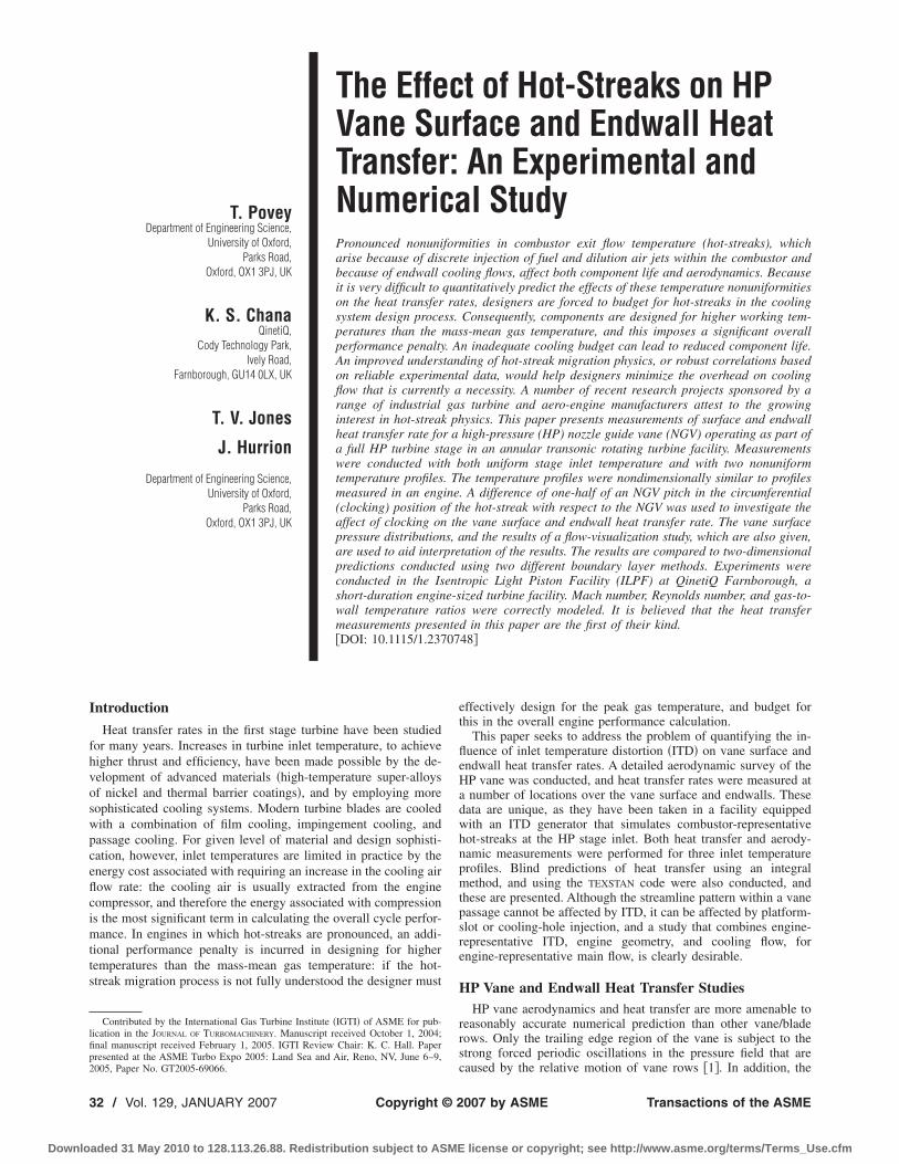
T. PoveyDepartment of Engineering Science,

University of Oxford,Parks Road,

Oxford, OX1 3PJ, UK

K. S. ChanaQinetiQ,

Cody Technology Park,Ively Road,

Farnborough, GU14 0LX, UK

T. V. Jones

J. Hurrion

Department of Engineering Science,University of Oxford,

Parks Road,Oxford, OX1 3PJ, UK

The Effect of Hot-Streaks on HPVane Surface and Endwall HeatTransfer: An Experimental andNumerical StudyPronounced nonuniformities in combustor exit flow temperature (hot-streaks), whicharise because of discrete injection of fuel and dilution air jets within the combustor andbecause of endwall cooling flows, affect both component life and aerodynamics. Becauseit is very difficult to quantitatively predict the effects of these temperature nonuniformitieson the heat transfer rates, designers are forced to budget for hot-streaks in the coolingsystem design process. Consequently, components are designed for higher working tem-peratures than the mass-mean gas temperature, and this imposes a significant overallperformance penalty. An inadequate cooling budget can lead to reduced component life.An improved understanding of hot-streak migration physics, or robust correlations basedon reliable experimental data, would help designers minimize the overhead on coolingflow that is currently a necessity. A number of recent research projects sponsored by arange of industrial gas turbine and aero-engine manufacturers attest to the growinginterest in hot-streak physics. This paper presents measurements of surface and endwallheat transfer rate for a high-pressure (HP) nozzle guide vane (NGV) operating as part ofa full HP turbine stage in an annular transonic rotating turbine facility. Measurementswere conducted with both uniform stage inlet temperature and with two nonuniformtemperature profiles. The temperature profiles were nondimensionally similar to profilesmeasured in an engine. A difference of one-half of an NGV pitch in the circumferential(clocking) position of the hot-streak with respect to the NGV was used to investigate theaffect of clocking on the vane surface and endwall heat transfer rate. The vane surfacepressure distributions, and the results of a flow-visualization study, which are also given,are used to aid interpretation of the results. The results are compared to two-dimensionalpredictions conducted using two different boundary layer methods. Experiments wereconducted in the Isentropic Light Piston Facility (ILPF) at QinetiQ Farnborough, ashort-duration engine-sized turbine facility. Mach number, Reynolds number, and gas-to-wall temperature ratios were correctly modeled. It is believed that the heat transfermeasurements presented in this paper are the first of their kind.�DOI: 10.1115/1.2370748�

Introduction

Heat transfer rates in the first stage turbine have been studiedfor many years. Increases in turbine inlet temperature, to achievehigher thrust and efficiency, have been made possible by the de-velopment of advanced materials �high-temperature super-alloysof nickel and thermal barrier coatings�, and by employing moresophisticated cooling systems. Modern turbine blades are cooledwith a combination of film cooling, impingement cooling, andpassage cooling. For given level of material and design sophisti-cation, however, inlet temperatures are limited in practice by theenergy cost associated with requiring an increase in the cooling airflow rate: the cooling air is usually extracted from the enginecompressor, and therefore the energy associated with compressionis the most significant term in calculating the overall cycle perfor-mance. In engines in which hot-streaks are pronounced, an addi-tional performance penalty is incurred in designing for highertemperatures than the mass-mean gas temperature: if the hot-streak migration process is not fully understood the designer must

effectively design for the peak gas temperature, and budget forthis in the overall engine performance calculation.

This paper seeks to address the problem of quantifying the in-fluence of inlet temperature distortion �ITD� on vane surface andendwall heat transfer rates. A detailed aerodynamic survey of theHP vane was conducted, and heat transfer rates were measured ata number of locations over the vane surface and endwalls. Thesedata are unique, as they have been taken in a facility equippedwith an ITD generator that simulates combustor-representativehot-streaks at the HP stage inlet. Both heat transfer and aerody-namic measurements were performed for three inlet temperatureprofiles. Blind predictions of heat transfer using an integralmethod, and using the TEXSTAN code were also conducted, andthese are presented. Although the streamline pattern within a vanepassage cannot be affected by ITD, it can be affected by platform-slot or cooling-hole injection, and a study that combines engine-representative ITD, engine geometry, and cooling flow, forengine-representative main flow, is clearly desirable.

HP Vane and Endwall Heat Transfer StudiesHP vane aerodynamics and heat transfer are more amenable to

reasonably accurate numerical prediction than other vane/bladerows. Only the trailing edge region of the vane is subject to thestrong forced periodic oscillations in the pressure field that arecaused by the relative motion of vane rows �1�. In addition, the

Contributed by the International Gas Turbine Institute �IGTI� of ASME for pub-lication in the JOURNAL OF TURBOMACHINERY. Manuscript received October 1, 2004;final manuscript received February 1, 2005. IGTI Review Chair: K. C. Hall. Paperpresented at the ASME Turbo Expo 2005: Land Sea and Air, Reno, NV, June 6–9,2005, Paper No. GT2005-69066.



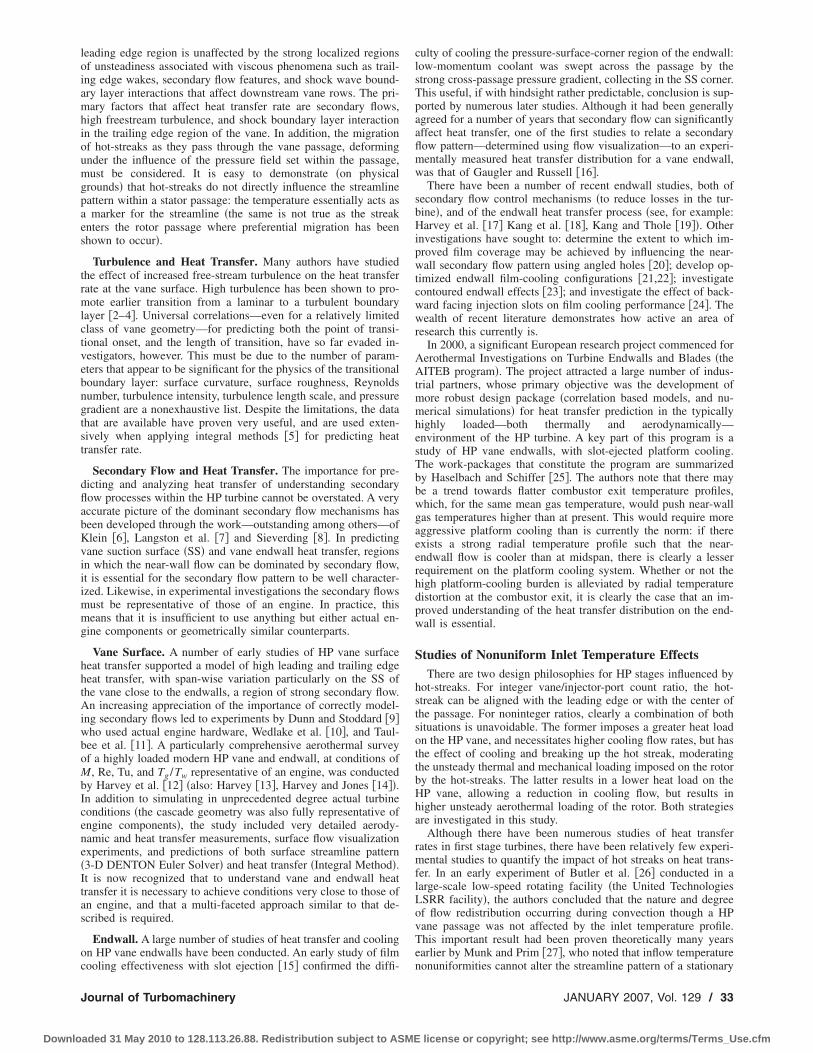
leading edge region is unaffected by the strong localized regionsof unsteadiness associated with viscous phenomena such as trail-ing edge wakes, secondary flow features, and shock wave bound-ary layer interactions that affect downstream vane rows. The pri-mary factors that affect heat transfer rate are secondary flows,high freestream turbulence, and shock boundary layer interactionin the trailing edge region of the vane. In addition, the migrationof hot-streaks as they pass through the vane passage, deformingunder the influence of the pressure field set within the passage,must be considered. It is easy to demonstrate �on physicalgrounds� that hot-streaks do not directly influence the streamlinepattern within a stator passage: the temperature essentially acts asa marker for the streamline �the same is not true as the streakenters the rotor passage where preferential migration has beenshown to occur�.

Turbulence and Heat Transfer. Many authors have studiedthe effect of increased free-stream turbulence on the heat transferrate at the vane surface. High turbulence has been shown to pro-mote earlier transition from a laminar to a turbulent boundarylayer �2–4�. Universal correlations—even for a relatively limitedclass of vane geometry—for predicting both the point of transi-tional onset, and the length of transition, have so far evaded in-vestigators, however. This must be due to the number of param-eters that appear to be significant for the physics of the transitionalboundary layer: surface curvature, surface roughness, Reynoldsnumber, turbulence intensity, turbulence length scale, and pressuregradient are a nonexhaustive list. Despite the limitations, the datathat are available have proven very useful, and are used exten-sively when applying integral methods �5� for predicting heattransfer rate.

Secondary Flow and Heat Transfer. The importance for pre-dicting and analyzing heat transfer of understanding secondaryflow processes within the HP turbine cannot be overstated. A veryaccurate picture of the dominant secondary flow mechanisms hasbeen developed through the work—outstanding among others—ofKlein �6�, Langston et al. �7� and Sieverding �8�. In predictingvane suction surface �SS� and vane endwall heat transfer, regionsin which the near-wall flow can be dominated by secondary flow,it is essential for the secondary flow pattern to be well character-ized. Likewise, in experimental investigations the secondary flowsmust be representative of those of an engine. In practice, thismeans that it is insufficient to use anything but either actual en-gine components or geometrically similar counterparts.

Vane Surface. A number of early studies of HP vane surfaceheat transfer supported a model of high leading and trailing edgeheat transfer, with span-wise variation particularly on the SS ofthe vane close to the endwalls, a region of strong secondary flow.An increasing appreciation of the importance of correctly model-ing secondary flows led to experiments by Dunn and Stoddard �9�who used actual engine hardware, Wedlake et al. �10�, and Taul-bee et al. �11�. A particularly comprehensive aerothermal surveyof a highly loaded modern HP vane and endwall, at conditions ofM, Re, Tu, and Tg /Tw representative of an engine, was conductedby Harvey et al. �12� �also: Harvey �13�, Harvey and Jones �14��.In addition to simulating in unprecedented degree actual turbineconditions �the cascade geometry was also fully representative ofengine components�, the study included very detailed aerody-namic and heat transfer measurements, surface flow visualizationexperiments, and predictions of both surface streamline pattern�3-D DENTON Euler Solver� and heat transfer �Integral Method�.It is now recognized that to understand vane and endwall heattransfer it is necessary to achieve conditions very close to those ofan engine, and that a multi-faceted approach similar to that de-scribed is required.

Endwall. A large number of studies of heat transfer and coolingon HP vane endwalls have been conducted. An early study of filmcooling effectiveness with slot ejection �15� confirmed the diffi-

culty of cooling the pressure-surface-corner region of the endwall:low-momentum coolant was swept across the passage by thestrong cross-passage pressure gradient, collecting in the SS corner.This useful, if with hindsight rather predictable, conclusion is sup-ported by numerous later studies. Although it had been generallyagreed for a number of years that secondary flow can significantlyaffect heat transfer, one of the first studies to relate a secondaryflow pattern—determined using flow visualization—to an experi-mentally measured heat transfer distribution for a vane endwall,was that of Gaugler and Russell �16�.

There have been a number of recent endwall studies, both ofsecondary flow control mechanisms �to reduce losses in the tur-bine�, and of the endwall heat transfer process �see, for example:Harvey et al. �17� Kang et al. �18�, Kang and Thole �19��. Otherinvestigations have sought to: determine the extent to which im-proved film coverage may be achieved by influencing the near-wall secondary flow pattern using angled holes �20�; develop op-timized endwall film-cooling configurations �21,22�; investigatecontoured endwall effects �23�; and investigate the effect of back-ward facing injection slots on film cooling performance �24�. Thewealth of recent literature demonstrates how active an area ofresearch this currently is.

In 2000, a significant European research project commenced forAerothermal Investigations on Turbine Endwalls and Blades �theAITEB program�. The project attracted a large number of indus-trial partners, whose primary objective was the development ofmore robust design package �correlation based models, and nu-merical simulations� for heat transfer prediction in the typicallyhighly loaded—both thermally and aerodynamically—environment of the HP turbine. A key part of this program is astudy of HP vane endwalls, with slot-ejected platform cooling.The work-packages that constitute the program are summarizedby Haselbach and Schiffer �25�. The authors note that there maybe a trend towards flatter combustor exit temperature profiles,which, for the same mean gas temperature, would push near-wallgas temperatures higher than at present. This would require moreaggressive platform cooling than is currently the norm: if thereexists a strong radial temperature profile such that the near-endwall flow is cooler than at midspan, there is clearly a lesserrequirement on the platform cooling system. Whether or not thehigh platform-cooling burden is alleviated by radial temperaturedistortion at the combustor exit, it is clearly the case that an im-proved understanding of the heat transfer distribution on the end-wall is essential.

Studies of Nonuniform Inlet Temperature EffectsThere are two design philosophies for HP stages influenced by

hot-streaks. For integer vane/injector-port count ratio, the hot-streak can be aligned with the leading edge or with the center ofthe passage. For noninteger ratios, clearly a combination of bothsituations is unavoidable. The former imposes a greater heat loadon the HP vane, and necessitates higher cooling flow rates, but hasthe effect of cooling and breaking up the hot streak, moderatingthe unsteady thermal and mechanical loading imposed on the rotorby the hot-streaks. The latter results in a lower heat load on theHP vane, allowing a reduction in cooling flow, but results inhigher unsteady aerothermal loading of the rotor. Both strategiesare investigated in this study.

Although there have been numerous studies of heat transferrates in first stage turbines, there have been relatively few experi-mental studies to quantify the impact of hot streaks on heat trans-fer. In an early experiment of Butler et al. �26� conducted in alarge-scale low-speed rotating facility �the United TechnologiesLSRR facility�, the authors concluded that the nature and degreeof flow redistribution occurring during convection though a HPvane passage was not affected by the inlet temperature profile.This important result had been proven theoretically many yearsearlier by Munk and Prim �27�, who noted that inflow temperaturenonuniformities cannot alter the streamline pattern of a stationary



blade row, the latter being influenced only by inlet total pressurenonuniformities. It is important not to infer—incorrectly—fromthis statement that mixing does not occur within the passage. It istrue only that ITD does not give rise to additional mixing.

It is the case, therefore, that changes in heat transfer associatedwith the introduction of temperature nonuniformity �for the samemean temperature� arise, in the case an HP vane passage, becauseof changes in driving temperature rather a change in heat transfercoefficient. The results of the first truly comprehensive study ofheat transfer on an HP vane and endwall with and without tem-perature nonuniformity �28� support this assertion. Measurementswere performed with the hot-streak aligned with the leading edgeof the vane, and aligned with the vane mid passage. This paperpresents a summary of those results. The measurements weretaken in a rotating annular turbine facility �the Isentropic LightPiston Facility at QinetiQ, Farnborough, UK� in which M, Re, Tu,and Tg /Tw were all correctly modeled, as was the geometry. TheHP vane count was 32, and 32 hot-streaks were simulated. Themeasurements are the first of their kind, to the authors’ knowl-edge.

The HP vane of the present study was operated as part of acomplete stage, and, later, as part of a 1.5 stage turbine with adownstream IP vane. The effect of hot-streaks both on the down-stream rotor and on the IP vane has been studied. The results ofthese investigations are reported in companion papers by Povey etal. �29�, for the case of the IP vane, and Chana and Jones �30�, forthe case of the HP rotor. While the result of Munk and Prim �27�holds for all blade/vane rows, for flow passing between vane/blade rows which are in relative motion, the inlet total pressurefields and incidence angles are altered by the introduction of ITD.Because of this effect, both the inviscid flow and the secondaryflow structures are altered. In this case, it is very difficult to sepa-rate the changes in heat transfer that arise because of changes inheat transfer coefficient, and those that arise because of changes inthe local driving temperature, even if, in some cases, there may begood reason to suspect that one of these processes is dominant. �Itis experimentally very difficult, especially in the case of nonuni-form inlet temperature, to deduce the local gas temperature withsufficient resolution and accuracy to resolve this question of pre-dominance.�

There are examples from engine test experience of local over-heating within the HP turbine, and on the HP rotor pressure sur-face �PS� and blade tip in particular. These effects are difficult toexplain without invoking hot-streak migration within the turbine.A number of studies of hot-streak migration within the HP turbineblade passage have been conducted, and the effect is now reason-ably well understood. The principal effect is incidence angle in-duced temperature segregation �26,31,32�, which can lead to pref-erential migration of hotter gas towards the PS of the rotor blade.

That there is growing interest in the effects of nonuniform inlettemperature on turbine heat transfer is evidenced by the number of

programs developed to study these effects. Experimental pro-grams in five different rotating facilities have been recorded. Inchronological order of first publication these are:

�i� The Warm Core Turbine Test Facility at the NASA LewisResearch Center, Cleveland, Ohio, USA �33,34�.

�ii� The Low Speed Rotating Rig �LSRR� at the United Tech-nologies Research Center, East Hartford, Connecticut,USA �26,35�.

�iii� The Rotating Blow-down Facility at the Massachusetts In-stitute of Technology, Cambridge, Massachusetts, USA�31,32�.

�iv� The Isentropic Light Piston turbine-test Facility �ILPF� atQinetiQ, Farnborough, Hampshire, UK �28,30�.

�v� The Turbine Research Facility �TRF� at the Wright-Patterson Air Force Base, Dayton, Ohio, USA �36�.

Hot-streak experiments have also been conducted in non-rotating facilities. Varadarajan and Bogard �37� �see also Jenkinsand Bogard �38�� measured adiabatic effectiveness on the SS of afilm-cooled nozzle guide vane for uniform inlet temperature andfor a hot-streak incident on the leading edge of the vane. Experi-ments were conducted in a large-scale two-dimensional cascade oftwo vane passages �at The University of Texas at Austin, Austin,Texas, USA�. Re was correctly modeled, but, because a linearcascade was used, the effect of realistic secondary flows could notbe quantified. Investigations of the effects of mainstream turbu-lence on the vane film cooling and hot-streak dispersion wereconducted in the same facility �39�.

In addition to experimental studies, there have been a largenumber of numerical studies to investigate the aerothermal, aero-dynamic, and aeromechanical impact of hot streaks in the high-pressure turbine. Publications in the period 2000 to 2004 include:Busby et al. �40�, Dorney and Sondak �41�, Gundy-Burlet andDorney �42�, Orkwis et al. �43�, Prasad and Hendricks �44�, Donget al. �45�, Hurrion �28�, Sondak et al. �46�, and He et al. �47�.

The Isentropic Light Piston FacilityThe ILPF is a short duration wind tunnel, capable of testing an

engine size turbine at the correct nondimensional parameters forfluid mechanics and heat transfer. The facility has been used totest both a single HP turbine stage �48� and a 1.5 turbine stageturbine �49�. For the experiments described in this paper, only theHP stage was installed. During a run M, Re, Tu, and Tg /Tw are allrepresentative of engine conditions. A novel feature of the facilityis the aerodynamic turbo-brake �50�, which is on the same shaft asthe turbine and is driven by the turbine exit-flow. At the designspeed, the turbobrake power is matched with the turbine, and thusconstant speed is maintained during a run. A schematic of thefacility is presented in Fig. 1. Air from a high-pressure reservoirdrives a piston down a piston tube, isentropically compressing and

Fig. 1 Schematic of the ILPF



heating the working gas �air� inside the tube. When the desiredpressure is reached, the compressed air is suddenly discharged, bymeans of a fast acting valve, into the working section. Typically,steady conditions are achieved for 500 ms.

The working section of the facility is shown diagrammaticallyin Fig. 2. The desired turbine pressure ratio is set by means of anadjustable second throat.

The design operating conditions of the ILPF are given in Table1. Measurements confirmed that the same stage inlet conditionswere achieved both with and without ITD.

Temperature Distortion FactorsMeasurements of temperature at the exit-plane of combustors

show large radial and circumferential variations in temperature.The flow is, in addition, highly unsteady. The time-mean tempera-ture field measured at the exit plane of a combustor typical of amodern military engine is presented in Fig. 3. Peak temperaturesare in excess of 2200 K, while at the hub and casing endwallsthere are relatively cool regions of flow, with temperatures as lowas 1500 K. Circumferential variations �hot-spots� arise because ofthe discrete nature of fuel and dilution air jets. In addition, com-bustor lining coolant flow causes a strong radial temperature gra-dient.

To quantify temperature nonuniformity, temperature distortionfactors �TDFs� are used. There are several definitions in currentuse, many of which are essentially the same. Combustor flow ishighly turbulent, and, because hot and cold gas streams are subjectto aggressive mixing, typical time-mean combustor exit tempera-ture profiles are generally rather smooth spatially. It may be suf-ficient, therefore, to describe an ITD with a single numerical

value. A distinction is sometimes drawn, however, between theoverall TDF �OTDF�, which is a measure of the divergence of thehottest gas streak from the mean temperature, and the radial TDF�RTDF�, which is a measure of the nonuniformity of the circum-ferentially averaged temperature field. The definitions that areused are as follows:

OTDF =Tmax − Tarea

�Tcomb, RTDF =

Tmaxcirc − Tarea

�Tcomb

where Tarea is the area mean temperature, Tcirc is the circumferen-tial mean temperature �expressed as a function of radial height�,�Tcomb is the temperature rise across the combustor, and T is thelocal temperature �a function of span, or area�. The subscript“max” identifies that the maximum of the quantity has been taken.Where a description of the form of the profile is required, the localOTDF �LOTDF� and local RTDF �LRTDF� forms follow natu-rally:

LOTDF =T − Tarea

�Tcomb, LRTDF =

Tcirc − Tarea

�Tcomb

The usefulness of these TDF definitions is not universally under-stood. In the engine situation, the parameter quantifies how com-pletely hot and cold gas streams mix. There is no direct analogy inthe test-facility situation. It is worth noting, however, that, where

heat transfer similarity is concerned, and where both Tarea /Tw andTcool /Tw �where Tcool is the temperature of the cold gas introducedto simulate ITD in the test rig situation�, equivalent TDFs may bedefined.

Fig. 2 The working section of the ILPF: HP turbine stage andturbobrake

Table 1 Operating point of the HP turbine stage with and with-out ITD.

Parameter

Predicteduniform

inlettemperature

Measured:Uniform

inlettemperature

Measured:ITD

p01, bar 4.6 4.6±2% 4.6±2%T01, K 444 444±2% 444±2%M2

hub 1.054 1.034±2% 1.063±2%M2

case 0.912 0.925±2% 0.926±2%�, r.p.m. 9500 9500±2% 9500±2%p3

hub, bar 1.434 1.428±2% 1.451±2%p3

case, bar 1.439 1.435±2% 1.453±2%p02r, bar 2.697 2.707±2% No data

Fig. 3 Typical measured combustor exit temperature profile



LOTDFrig =T − Tarea

Tarea − Tcool

, LRTDFrig =Tcirc − Tarea

Tarea − Tcool

It can be shown that if LOTDFrig �rig situation� is matched toLOTDF �engine situation�, the nondimensional vane inlet tem-

perature profile �T / Tarea� will also be approximately matched.This is so whether or not there is similarity of mixing processes�rig to engine� upstream of the vane inlet plane.

The Temperature Distortion GeneratorIn a typical civil engine, fuel-injector-to-vane-count ratios near

1:2 are not uncommon. Count ratios are often noninteger, how-ever, and therefore the possible benefits associated with hot-streakclocking are difficult to realize in practice. HP vane surface cool-ing systems must be designed for peak combustor exit tempera-tures. There has been, therefore, considerable interested in theeffects of hot streak clocking �relative circumferential position�.

The ITD generator used in the ILPF is described in detail byChana et al. �51�. Hot-streaks, rotatable with respect to the NGVleading edge, are generated by blowing cool air through strutsupstream of the HP NGVs. The number of hot streaks was thesame as the HP vane count: 32. Experimental results for twoclocking positions are discussed in this paper. The temperatureprofiles measured at the inlet plane of the HP vane �average ofarea surveys at three locations around the annulus� are presentedin Fig. 4. The scale is presented both as time-mean temperature,

and as temperature ratio, T / Tarea: it is worth noting that wherehot-streak migration physics is concerned, it is sufficient to match

T / Tarea alone, although a number of parameters—essentiallyidentical—have been used by other authors. The two profiles forwhich data is presented are referred to as OTDF1 �hot-streakaligned geometrically with the vane midpassage� and OTDF2�hot-streak aligned with the vane leading edge�. Thus, the effect ofclocking the hot-streak with respect to the HP vane could be in-vestigated.

The maximum and minimum measured gas temperatures wereapproximately 480 and 412 K �note that measurements were notconducted very close to the wall—within 5% span of the end-wall�. The mean temperature was the same for both uniform andnonuniform inlet temperature: 444 K. Because cool air was in-jected to create an ITD, a higher main flow temperature was re-quired. This was achieved by increasing the pump-tube compres-sion ratio. The peak-to-mean and minimum-to-mean temperatureratios were approximately 1.08 and 0.93, respectively.

There was no significant difference between the radial tempera-

ture profiles �circumferentially averaged�, Tcirc / Tarea, for OTDF1and OTDF2. The measured radial profile is presented in Fig. 5 andis compared to the temperature profile of a typical engine �mea-surements were not taken very close to the endwall—within 5%span of the endwall—and the temperature at the nearest point wasused in this region�. The measured temperature profile withoutITD is also given, and is indicated in Fig. 5 by “Measured Uni-form.” The measured radial profiles for OTDF1 and OTDF2 werevery similar in both magnitude and form to the engine profile. The

peak measured value of Tcirc / Tarea was 1.045, while the peak en-

gine value was 1.055. The minimum measured value of Tcirc / Tarea

was 0.93, while the corresponding engine value was 0.89. Thereare many ways of comparing the intensities of peaks of nonuni-form temperature profiles. A useful comparison may be made interms of a nondimensional intensity factor such as the ratio �rig-to-engine� of nondimensionalzed peak-to-min temperature differ-ences in the radial profile:

�Tmaxcirc /Tarea − Tmin

circ/Tarea�rig

�Tmaxcirc /Tarea − Tmin

circ/Tarea�engine

In terms of this parameter, the ratio was approximately 0.7:1.0.The nondimensional temperature field of the experiment wastherefore similar in magnitude to that of a typical engine.

Instrumentation and ProcessingThe HP vane was instrumented with static pressure tappings at

10, 50, and 90% spans on both the pressure and suction surface ofthe vane. Surface heat transfer measurements were conducted us-ing thin-film platinum resistance heat transfer gauges of the typedescribed by Oldfield and Doorly �52�. On the vane pressure andsuction surfaces, a thin Upilex™—polyimide—substrate was usedto support the gauges, as shown in Fig. 6 �two-layer substrate�. Toconduct measurements on the endwalls, gauges were painted andfired directly onto vanes made from Macor™, a machinable glass,as shown in Fig. 7 �single-layer substrate�.

Uncertainty in Nusselt Number. Equations for the transientthermal response of a thin-film gauge on a two-layer substrate arepresented by Doorly and Oldfield �53�. The corresponding equa-tions for a single-layer substrate are given by, for example, Jones�54�. A full uncertainty analysis for thin-film heat transfer mea-surements is quite involved. Povey �55�, considers the followingsources of uncertainty:

Fig. 4 Measured inlet temperature profiles: OTDF1 and OTDF2

Fig. 5 Comparison of the ILPF radial temperature profile withtypical engine profile



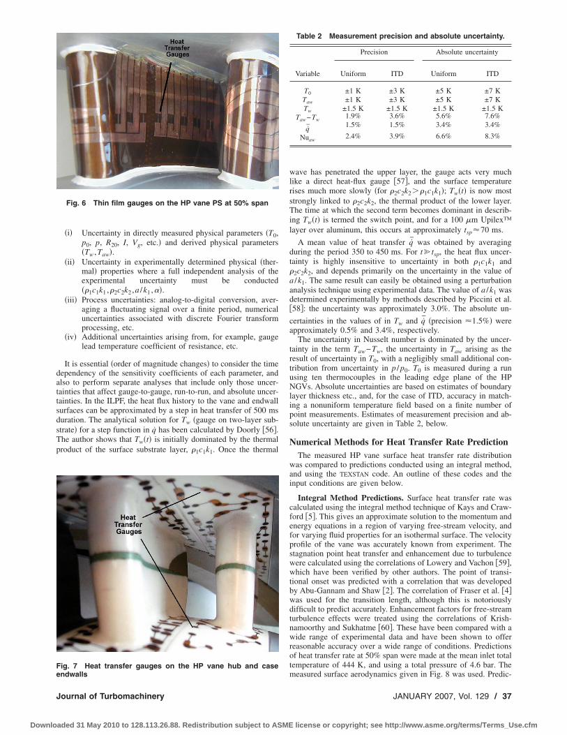
�i� Uncertainty in directly measured physical parameters �T0,p0, p, R20, I, Vg, etc.� and derived physical parameters�Tw ,Taw�.

�ii� Uncertainty in experimentally determined physical �ther-mal� properties where a full independent analysis of theexperimental uncertainty must be conducted��1c1k1 ,�2c2k2 ,a /k1 ,��.

�iii� Process uncertainties: analog-to-digital conversion, aver-aging a fluctuating signal over a finite period, numericaluncertainties associated with discrete Fourier transformprocessing, etc.

�iv� Additional uncertainties arising from, for example, gaugelead temperature coefficient of resistance, etc.

It is essential �order of magnitude changes� to consider the timedependency of the sensitivity coefficients of each parameter, andalso to perform separate analyses that include only those uncer-tainties that affect gauge-to-gauge, run-to-run, and absolute uncer-tainties. In the ILPF, the heat flux history to the vane and endwallsurfaces can be approximated by a step in heat transfer of 500 msduration. The analytical solution for Tw �gauge on two-layer sub-strate� for a step function in q has been calculated by Doorly �56�.The author shows that Tw�t� is initially dominated by the thermalproduct of the surface substrate layer, �1c1k1. Once the thermal

wave has penetrated the upper layer, the gauge acts very muchlike a direct heat-flux gauge �57�, and the surface temperaturerises much more slowly �for �2c2k2��1c1k1�; Tw�t� is now moststrongly linked to �2c2k2, the thermal product of the lower layer.The time at which the second term becomes dominant in describ-ing Tw�t� is termed the switch point, and for a 100 �m Upilex™layer over aluminum, this occurs at approximately tsp�70 ms.

A mean value of heat transfer q was obtained by averagingduring the period 350 to 450 ms. For t� tsp, the heat flux uncer-tainty is highly insensitive to uncertainty in both �1c1k1 and�2c2k2, and depends primarily on the uncertainty in the value ofa /k1. The same result can easily be obtained using a perturbationanalysis technique using experimental data. The value of a /k1 wasdetermined experimentally by methods described by Piccini et al.�58�: the uncertainty was approximately 3.0%. The absolute un-

certainties in the values of in Tw and q �precision �1.5%� wereapproximately 0.5% and 3.4%, respectively.

The uncertainty in Nusselt number is dominated by the uncer-tainty in the term Taw−Tw, the uncertainty in Taw arising as theresult of uncertainty in T0, with a negligibly small additional con-tribution from uncertainty in p / p0. T0 is measured during a runusing ten thermocouples in the leading edge plane of the HPNGVs. Absolute uncertainties are based on estimates of boundarylayer thickness etc., and, for the case of ITD, accuracy in match-ing a nonuniform temperature field based on a finite number ofpoint measurements. Estimates of measurement precision and ab-solute uncertainty are given in Table 2, below.

Numerical Methods for Heat Transfer Rate PredictionThe measured HP vane surface heat transfer rate distribution

was compared to predictions conducted using an integral method,and using the TEXSTAN code. An outline of these codes and theinput conditions are given below.

Integral Method Predictions. Surface heat transfer rate wascalculated using the integral method technique of Kays and Craw-ford �5�. This gives an approximate solution to the momentum andenergy equations in a region of varying free-stream velocity, andfor varying fluid properties for an isothermal surface. The velocityprofile of the vane was accurately known from experiment. Thestagnation point heat transfer and enhancement due to turbulencewere calculated using the correlations of Lowery and Vachon �59�,which have been verified by other authors. The point of transi-tional onset was predicted with a correlation that was developedby Abu-Gannam and Shaw �2�. The correlation of Fraser et al. �4�was used for the transition length, although this is notoriouslydifficult to predict accurately. Enhancement factors for free-streamturbulence effects were treated using the correlations of Krish-namoorthy and Sukhatme �60�. These have been compared with awide range of experimental data and have been shown to offerreasonable accuracy over a wide range of conditions. Predictionsof heat transfer rate at 50% span were made at the mean inlet totaltemperature of 444 K, and using a total pressure of 4.6 bar. Themeasured surface aerodynamics given in Fig. 8 was used. Predic-

Fig. 6 Thin film gauges on the HP vane PS at 50% span

Fig. 7 Heat transfer gauges on the HP vane hub and caseendwalls

Table 2 Measurement precision and absolute uncertainty.

Variable

Precision Absolute uncertainty

Uniform ITD Uniform ITD

T0 ±1 K ±3 K ±5 K ±7 KTaw ±1 K ±3 K ±5 K ±7 KTw ±1.5 K ±1.5 K ±1.5 K ±1.5 K

Taw−Tw1.9% 3.6% 5.6% 7.6%

q 1.5% 1.5% 3.4% 3.4%

Nuaw2.4% 3.9% 6.6% 8.3%



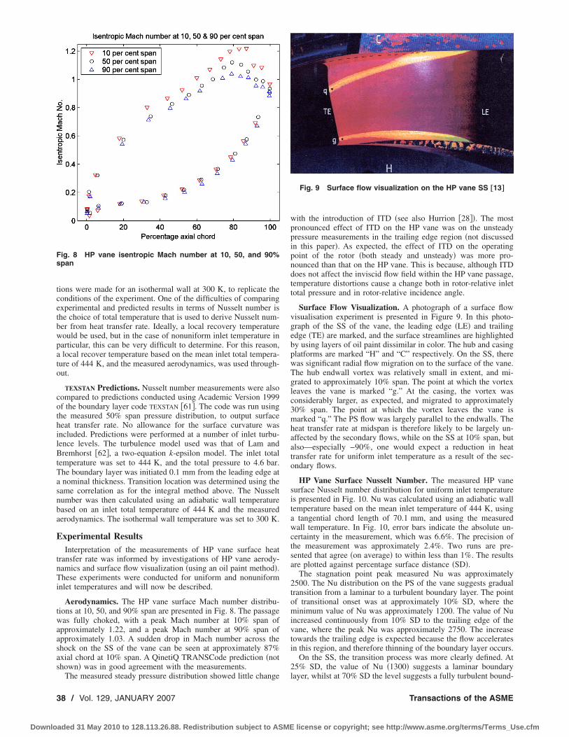
tions were made for an isothermal wall at 300 K, to replicate theconditions of the experiment. One of the difficulties of comparingexperimental and predicted results in terms of Nusselt number isthe choice of total temperature that is used to derive Nusselt num-ber from heat transfer rate. Ideally, a local recovery temperaturewould be used, but in the case of nonuniform inlet temperature inparticular, this can be very difficult to determine. For this reason,a local recover temperature based on the mean inlet total tempera-ture of 444 K, and the measured aerodynamics, was used through-out.

TEXSTAN Predictions. Nusselt number measurements were alsocompared to predictions conducted using Academic Version 1999of the boundary layer code TEXSTAN �61�. The code was run usingthe measured 50% span pressure distribution, to output surfaceheat transfer rate. No allowance for the surface curvature wasincluded. Predictions were performed at a number of inlet turbu-lence levels. The turbulence model used was that of Lam andBremhorst �62�, a two-equation k-epsilon model. The inlet totaltemperature was set to 444 K, and the total pressure to 4.6 bar.The boundary layer was initiated 0.1 mm from the leading edge ata nominal thickness. Transition location was determined using thesame correlation as for the integral method above. The Nusseltnumber was then calculated using an adiabatic wall temperaturebased on an inlet total temperature of 444 K and the measuredaerodynamics. The isothermal wall temperature was set to 300 K.

Experimental ResultsInterpretation of the measurements of HP vane surface heat

transfer rate was informed by investigations of HP vane aerody-namics and surface flow visualization �using an oil paint method�.These experiments were conducted for uniform and nonuniforminlet temperatures and will now be described.

Aerodynamics. The HP vane surface Mach number distribu-tions at 10, 50, and 90% span are presented in Fig. 8. The passagewas fully choked, with a peak Mach number at 10% span ofapproximately 1.22, and a peak Mach number at 90% span ofapproximately 1.03. A sudden drop in Mach number across theshock on the SS of the vane can be seen at approximately 87%axial chord at 10% span. A QinetiQ TRANSCode prediction �notshown� was in good agreement with the measurements.

The measured steady pressure distribution showed little change

with the introduction of ITD �see also Hurrion �28��. The mostpronounced effect of ITD on the HP vane was on the unsteadypressure measurements in the trailing edge region �not discussedin this paper�. As expected, the effect of ITD on the operatingpoint of the rotor �both steady and unsteady� was more pro-nounced than that on the HP vane. This is because, although ITDdoes not affect the inviscid flow field within the HP vane passage,temperature distortions cause a change both in rotor-relative inlettotal pressure and in rotor-relative incidence angle.

Surface Flow Visualization. A photograph of a surface flowvisualisation experiment is presented in Figure 9. In this photo-graph of the SS of the vane, the leading edge �LE� and trailingedge �TE� are marked, and the surface streamlines are highlightedby using layers of oil paint dissimilar in color. The hub and casingplatforms are marked “H” and “C” respectively. On the SS, therewas significant radial flow migration on to the surface of the vane.The hub endwall vortex was relatively small in extent, and mi-grated to approximately 10% span. The point at which the vortexleaves the vane is marked “g.” At the casing, the vortex wasconsiderably larger, as expected, and migrated to approximately30% span. The point at which the vortex leaves the vane ismarked “q.” The PS flow was largely parallel to the endwalls. Theheat transfer rate at midspan is therefore likely to be largely un-affected by the secondary flows, while on the SS at 10% span, butalso—especially −90%, one would expect a reduction in heattransfer rate for uniform inlet temperature as a result of the sec-ondary flows.

HP Vane Surface Nusselt Number. The measured HP vanesurface Nusselt number distribution for uniform inlet temperatureis presented in Fig. 10. Nu was calculated using an adiabatic walltemperature based on the mean inlet temperature of 444 K, usinga tangential chord length of 70.1 mm, and using the measuredwall temperature. In Fig. 10, error bars indicate the absolute un-certainty in the measurement, which was 6.6%. The precision ofthe measurement was approximately 2.4%. Two runs are pre-sented that agree �on average� to within less than 1%. The resultsare plotted against percentage surface distance �SD�.

The stagnation point peak measured Nu was approximately2500. The Nu distribution on the PS of the vane suggests gradualtransition from a laminar to a turbulent boundary layer. The pointof transitional onset was at approximately 10% SD, where theminimum value of Nu was approximately 1200. The value of Nuincreased continuously from 10% SD to the trailing edge of thevane, where the peak Nu was approximately 2750. The increasetowards the trailing edge is expected because the flow acceleratesin this region, and therefore thinning of the boundary layer occurs.

On the SS, the transition process was more clearly defined. At25% SD, the value of Nu �1300� suggests a laminar boundarylayer, whilst at 70% SD the level suggests a fully turbulent bound-

Fig. 8 HP vane isentropic Mach number at 10, 50, and 90%span

Fig. 9 Surface flow visualization on the HP vane SS †13‡



ary layer. From 70% SD to the trailing edge of the vane, the Nu isalmost constant �approximately 2500�. It is not possible to deter-mine the length of the transitional region exactly, but the availabledata place a maximum bound on the length of 45% SD; it is likelyto be significantly shorter than this.

Comparison of Measured HP Vane Surface Nusselt NumberWith TEXSTAN and Integral Method Predictions. The integralmethod prediction for HP vane surface Nusselt number distribu-tion is compared to the experimental data at 50% span in Fig. 11.Predictions were made for a free-stream turbulence level of 5%.Experimental points are marked as open circles. The blind predic-tion and the prediction for a fully laminar boundary layer arepresented. The latter is useful in comparing prediction and experi-ment in the transitional region.

The leading edge Nu number is in excellent agreement with theexperimental value. Similarly, the predicted Nu on the SS plateau�towards the trailing edge of the vane� is in reasonable agreementwith the measured results, the predicted value being approxi-mately 30% greater. On the PS of the vane, the predicted onsetand length of transition are in reasonable agreement with the ex-perimental results, although the predicted Nu distribution is some-what higher than the measured values from 30% SD onwards. It isclear that on the SS, however, the correlations for onset and lengthof transition do not accurately represent what was measured. Theprediction is for fully developed turbulent flow at 25% SD, whilethe experimental results suggest transitional flow at 50% SD.

Similarly, the prediction is for transitional onset at 10% SD, whilemeasurements suggest a fully laminar boundary layer at 25% SD.The large discrepancies between the measured and predicted dis-tributions of Nu on the SS arise because the transitional region ispoorly modeled. The results highlight a common problem in pre-dicting transitional behavior in regions of strong streamwise pres-sure gradient.

The same correlations as those used in the Integral Methodcode were used for prediction of transitional onset and length oftransition in the TEXSTAN code, resulting in similar discrepanciesbetween predicted and measured values. Imposing start and endpoints of transition resulted in good agreement between measuredand predicted values of Nu. The Integral Method and the TEXSTAN

predictions—for forced transition—are compared to the experi-mental measurements in Fig. 12. The TEXSTAN results are pre-sented using a gas temperature of 444 K �“Uncorrected”� and us-ing a recovery temperature based on a total temperature of 444 K�“Corrected”�. When the transition locations are imposed, the pre-dictions agree well with experimental results. On the SS, theTEXSTAN prediction is everywhere within 30% of the measuredresults, with the greatest discrepancy in the leading edge region.On the SS, the TEXSTAN and Integral Method predictions are verysimilar in magnitude and form. On the PS, the TEXSTAN predictionis somewhat closer to the experimental results than the IntegralMethod prediction and the discrepancy between TEXSTAN predic-tion and experiment was everywhere less than 20%.

Overall, the TEXSTAN prediction is in slightly better agreementwith the experimental results than the Integral Method, but bothcodes have similar limitations: in particular, the problem with theaccurate prediction of the point of transitional onset and the lengthof transitional region.

Comparison of HP Vane Surface Nusselt Number With andWithout Inlet Temperature Distortion. The measured Nusseltnumber at 50% span is presented in Fig. 13. Results are given foruniform inlet temperature, and for ITDs OTDF1 and OTDF2. Nuwas calculated using local recovery temperature based on a meaninlet temperature �444 K� and on the tangential chord of the vane.Error bars represent absolute uncertainty in the data points: 6.6%for uniform inlet temperature, and 8.3% for ITD. Precision �re-peatability� uncertainties were 2.4% and 3.9%, respectively, al-though in practice significantly better repeatability was obtainedbetween runs.

The stagnation point Nu was similar �within �10%� for uni-form inlet temperature and for ITD. The exact location of the peakis not significant, as different instrumentation was used for uni-form temperature and ITD measurements, and the number ofgauges was insufficient to determine exactly the location of thestagnation point. On the PS of the vane, there was little change in

Fig. 10 Measured HP vane surface Nusselt numberdistribution

Fig. 11 Integral Method prediction for HP vane surface Nucompared to experimental data

Fig. 12 Integral method and TEXSTAN predictions for HP vanesurface Nu compared to experimental data



Nu with ITD. Differences between the measurements were of theorder of 10% or lower. On the SS, in contrast, there was a markedchange with the introduction of ITD. On the SS, the general formof the measurements was similar for the three temperature pro-files: high Nu ��2500� at the leading edge stagnation point; areduction in Nu in the laminar boundary layer region; a rapidincrease in Nu as the flow undergoes transition; a plateau in Nutowards the trailing edge in the fully turbulent boundary layerregion. The measurements conducted for OTDF2 show that thevalue of Nu is consistently higher on the SS than for either uni-form inlet temperature or for OTDF1. In contrast, the measuredNu distribution for OTDF1 was similar to that for uniform inlettemperature over the early SS, but lower towards the trailing edgethan for either of the other two profiles.

The results are now discussed with reference to Figure 14,which is a schematic representation of the streamlines at 50%span for ITDs OTDF1 and OTDF2. In Fig. 14, a schematic crosssection of the temperature profile is presented, depicting theclocking position of the hot-streak with respect to the vane leadingedge. Regions of high, intermediate, and low temperature are in-dicated by red, green, and blue, respectively. Although the ITDgenerator was configured so that the hot-streaks were aligned—geometrically—with the HP vane midpassage �OTDF1�, and withthe vane leading edges �OTDF2�, circulation in the approach tothe vane leading edge region introduces a shift in the location ofthe peak with respect to the vane leading edge. The left side of thefigure is a schematic of OTDF1. Because of the effect of circula-tion, the low temperature region is not incident equally on the

pressure and suction surfaces of the vane, but moves towards theSS. Thus, there is a reduction in driving gas temperature only onthe SS of the vane: consider the results presented for OTDF1 inFig. 13. Likewise, for OTDF2, circulation causes the hot-streak toimpact the SS of the vane, rather than equally on both surfaces:consider the results presented for OTDF2 in Fig. 13. The resultsdemonstrate that the effect of ITD on heat transfer is significant,and highlight the necessity of correctly calculating the displace-ment effect of circulation ahead of the vanes if clocking is to beused to advantage in engine design.

Comparison of HP Vane Endwall Nusselt Number With andWithout Inlet Temperature Distortion. The midpassage Nu onthe HP vane hub endwall is shown in Fig. 15. Heat transfer mea-surements were conducted throughout the passage �approximately40 locations� and the data were fitted with a three-dimensionalspline. Nu based on mean inlet total temperature �T01=444 K�was then calculated from the spline fit. Results are presented foruniform inlet temperature, and for ITDs OTDF1 and OTDF2. Nuis plotted against percentage axial chord �0% =leading edge,100% =trailing edge�.

For uniform inlet temperature, the hub endwall Nu at inlet tothe vane passage was approximately 1400. Close to the trailingedge Nu plateaus at approximately 3000, then falls rapidly toapproximately 2300 downstream of the vane. Harvey �13� con-ducted similar measurements on the vane endwall, which are pre-sented for comparison. The data are in agreement, and this lendsconfidence to the results.

The results for OTDF1 and OTDF2 are very similar, and showa significant reduction—over the results for uniform inlettemperature—in midpassage Nu based on mean inlet temperature.Between 0 and 95% axial chord the reduction in Nu is between 30and 50%. The reduction in Nu �as defined above� implies either areduction in driving temperature, or a reduction in the heat trans-fer coefficient. These effects are, in fact, impossible to separate,and this highlights a common problem with heat transfer investi-gations. The aerodynamic survey �presented above� gave strongevidence, however, that there was little change with ITD in thevane flow-field. This is in accord with the theoretical result ofMunk and Prim �27�, which states that no additional redistributionof the mainstream flow �because here viscous forces are negli-gible� is expected with ITD. It seems likely, therefore, that theobserved change in Nu is largely driving-temperature-induced,rather than caused by a change in heat transfer coefficient. Thereduction of Nu on the hub endwall suggests that the mean gastemperature in the near-endwall region is lower for OTDF1 andOTDF2 than for uniform inlet temperature. This is expected, anddemonstrates the beneficial effect on endwall heat load of ITD. It

Fig. 13 Comparison of HP vane surface Nusselt number dis-tribution with and without ITD at 50% span

Fig. 14 Schematic of the 50 percent span streamlines forOTDF1 and OTDF2

Fig. 15 Nusselt number on the HP vane hub endwall with andwithout ITD



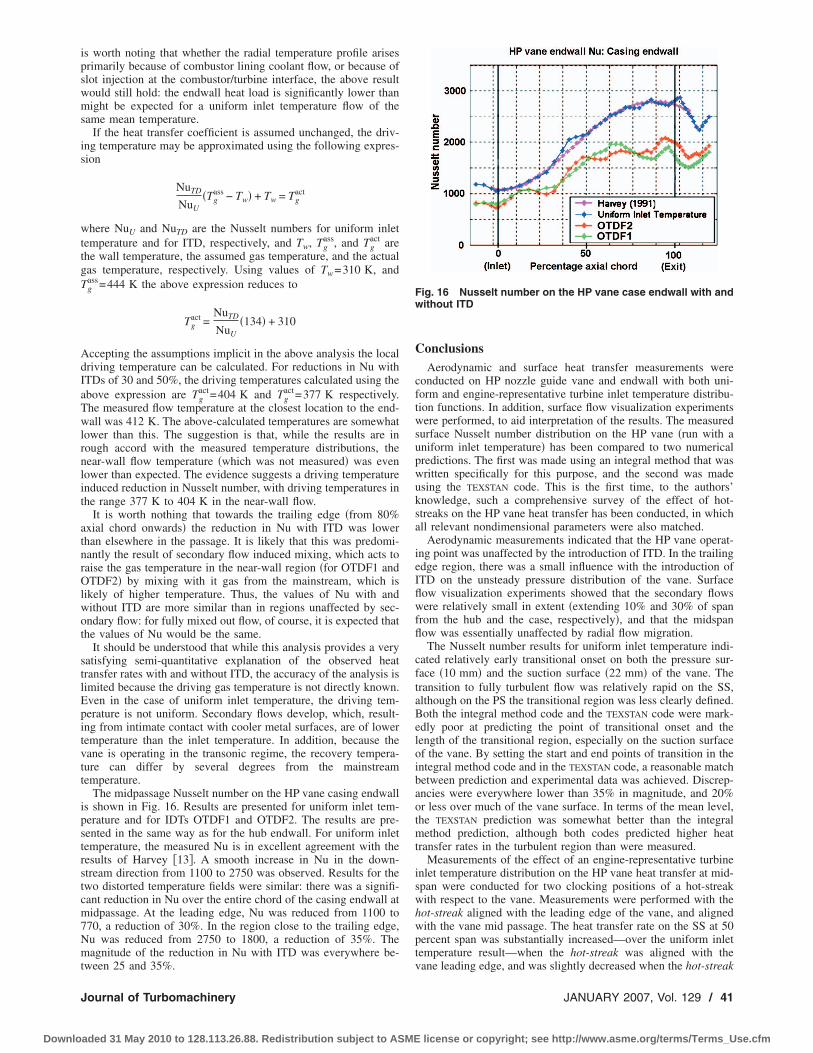
is worth noting that whether the radial temperature profile arisesprimarily because of combustor lining coolant flow, or because ofslot injection at the combustor/turbine interface, the above resultwould still hold: the endwall heat load is significantly lower thanmight be expected for a uniform inlet temperature flow of thesame mean temperature.

If the heat transfer coefficient is assumed unchanged, the driv-ing temperature may be approximated using the following expres-sion

NuTD

NuU�Tg

ass − Tw� + Tw = Tgact

where NuU and NuTD are the Nusselt numbers for uniform inlettemperature and for ITD, respectively, and Tw, Tg

ass, and Tgact are

the wall temperature, the assumed gas temperature, and the actualgas temperature, respectively. Using values of Tw=310 K, andTg

ass=444 K the above expression reduces to

Tgact =

NuTD

NuU�134� + 310

Accepting the assumptions implicit in the above analysis the localdriving temperature can be calculated. For reductions in Nu withITDs of 30 and 50%, the driving temperatures calculated using theabove expression are Tg

act=404 K and Tgact=377 K respectively.

The measured flow temperature at the closest location to the end-wall was 412 K. The above-calculated temperatures are somewhatlower than this. The suggestion is that, while the results are inrough accord with the measured temperature distributions, thenear-wall flow temperature �which was not measured� was evenlower than expected. The evidence suggests a driving temperatureinduced reduction in Nusselt number, with driving temperatures inthe range 377 K to 404 K in the near-wall flow.

It is worth nothing that towards the trailing edge �from 80%axial chord onwards� the reduction in Nu with ITD was lowerthan elsewhere in the passage. It is likely that this was predomi-nantly the result of secondary flow induced mixing, which acts toraise the gas temperature in the near-wall region �for OTDF1 andOTDF2� by mixing with it gas from the mainstream, which islikely of higher temperature. Thus, the values of Nu with andwithout ITD are more similar than in regions unaffected by sec-ondary flow: for fully mixed out flow, of course, it is expected thatthe values of Nu would be the same.

It should be understood that while this analysis provides a verysatisfying semi-quantitative explanation of the observed heattransfer rates with and without ITD, the accuracy of the analysis islimited because the driving gas temperature is not directly known.Even in the case of uniform inlet temperature, the driving tem-perature is not uniform. Secondary flows develop, which, result-ing from intimate contact with cooler metal surfaces, are of lowertemperature than the inlet temperature. In addition, because thevane is operating in the transonic regime, the recovery tempera-ture can differ by several degrees from the mainstreamtemperature.

The midpassage Nusselt number on the HP vane casing endwallis shown in Fig. 16. Results are presented for uniform inlet tem-perature and for IDTs OTDF1 and OTDF2. The results are pre-sented in the same way as for the hub endwall. For uniform inlettemperature, the measured Nu is in excellent agreement with theresults of Harvey �13�. A smooth increase in Nu in the down-stream direction from 1100 to 2750 was observed. Results for thetwo distorted temperature fields were similar: there was a signifi-cant reduction in Nu over the entire chord of the casing endwall atmidpassage. At the leading edge, Nu was reduced from 1100 to770, a reduction of 30%. In the region close to the trailing edge,Nu was reduced from 2750 to 1800, a reduction of 35%. Themagnitude of the reduction in Nu with ITD was everywhere be-tween 25 and 35%.

ConclusionsAerodynamic and surface heat transfer measurements were

conducted on HP nozzle guide vane and endwall with both uni-form and engine-representative turbine inlet temperature distribu-tion functions. In addition, surface flow visualization experimentswere performed, to aid interpretation of the results. The measuredsurface Nusselt number distribution on the HP vane �run with auniform inlet temperature� has been compared to two numericalpredictions. The first was made using an integral method that waswritten specifically for this purpose, and the second was madeusing the TEXSTAN code. This is the first time, to the authors’knowledge, such a comprehensive survey of the effect of hot-streaks on the HP vane heat transfer has been conducted, in whichall relevant nondimensional parameters were also matched.

Aerodynamic measurements indicated that the HP vane operat-ing point was unaffected by the introduction of ITD. In the trailingedge region, there was a small influence with the introduction ofITD on the unsteady pressure distribution of the vane. Surfaceflow visualization experiments showed that the secondary flowswere relatively small in extent �extending 10% and 30% of spanfrom the hub and the case, respectively�, and that the midspanflow was essentially unaffected by radial flow migration.

The Nusselt number results for uniform inlet temperature indi-cated relatively early transitional onset on both the pressure sur-face �10 mm� and the suction surface �22 mm� of the vane. Thetransition to fully turbulent flow was relatively rapid on the SS,although on the PS the transitional region was less clearly defined.Both the integral method code and the TEXSTAN code were mark-edly poor at predicting the point of transitional onset and thelength of the transitional region, especially on the suction surfaceof the vane. By setting the start and end points of transition in theintegral method code and in the TEXSTAN code, a reasonable matchbetween prediction and experimental data was achieved. Discrep-ancies were everywhere lower than 35% in magnitude, and 20%or less over much of the vane surface. In terms of the mean level,the TEXSTAN prediction was somewhat better than the integralmethod prediction, although both codes predicted higher heattransfer rates in the turbulent region than were measured.

Measurements of the effect of an engine-representative turbineinlet temperature distribution on the HP vane heat transfer at mid-span were conducted for two clocking positions of a hot-streakwith respect to the vane. Measurements were performed with thehot-streak aligned with the leading edge of the vane, and alignedwith the vane mid passage. The heat transfer rate on the SS at 50percent span was substantially increased—over the uniform inlettemperature result—when the hot-streak was aligned with thevane leading edge, and was slightly decreased when the hot-streak

Fig. 16 Nusselt number on the HP vane case endwall with andwithout ITD



was aligned with the vane midpassage. The same result was notobserved on the PS at 50% span, which was insensitive to changesin ITD. The results were explained qualitatively in terms of amodel that included the effect of circulation in the approach to thevane leading edge. The results demonstrate that hot-streaks canhave a significant impact on HP vane heat transfer, and highlightthe need to carefully characterize the streamline pattern in thisregion if the effects of clocking are included in the turbine designprocess.

Detailed measurements of the heat transfer rate to the HP vanepassage end-walls with and without ITD were conducted. Theresults for uniform inlet temperature were in excellent agreementwith measurements conducted in the same facility by Harvey�1991�; this was in support of the robustness of the measurements.With the introduction of ITD there was a large decrease in heattransfer rate over the entire endwall surface at both hub and thecasing. Along the mid-passage streamline, the decrease in Nu�based on mean inlet temperature� with ITD at the hub endwallwas between 30 and 50%. Along the casing endwall, the reductionwas between 25 and 35%. The reduction was very similar for bothclocking positions of the hot-streak, suggesting the effect is notaffected by the relative circumferential positions of the hot-streakand the HP vane. The form of the results �and other evidencediscussed in the text� suggested that the decrease in heat transferrate was the result of a lower local total temperature of the gasnear the endwalls rather than a decrease in the heat transfer coef-ficient. The driving gas temperatures were calculated by assumingthe same heat transfer coefficient as measured for uniform inlettemperature, and were in approximate agreement with tempera-tures measured close to the endwall at inlet to the vane. The re-sults demonstrate that ITD can have a very significant effect onthe endwall heat transfer.

AcknowledgmentsThe assistance of S. J. Anderson and A. H. Mole in the acqui-

sition of data contained in this report is gratefully acknowledged.This work was conducted as part of, and was funded under, theBrite Euram Forth Framework on Turbine Aerothermal ExternalFlows, Contract Number BRPR-CT97-0519. The UK Departmentof Trade and Industry through the CARAD Programme also pro-vided funding.

Nomenclaturea � thickness of Upilex™ �upper substrate�

layerc � specific heat capacityI � gauge supply �constant� currentk � thermal conductivity

M � isentropic Mach numberp ; p0 ; p01 � static pressure; total pressure; total pressure

at stage inletR20 � gauge resistance at 20°CRe � Reynolds numberTu � turbulence intensity

T0 ;T01 � total temperature; total temperature at stageinlet

Tcool � temperature of injected coolant flow

Tg� ;Tgass ;Tg

act � local gas temperature; assumed; actualTmax;�Tcomb � peak combustor exit temperature; tempera-

ture rise across combustorTw ;Taw � local wall temperature; adiabatic wall

temperature

Tarea � area mean temperature

Tcirc � circumferential mean temperature �ex-pressed as a function of radial height�

Vg � gauge output voltage� � temperature coefficient of resistance

� � material density� � angular speed of turbine

AbbreviationsHP � high-pressure

ITD � inlet temperature distortionNGV � nozzle guide vane

OTDF & RTDF � overall & radial temperature distortionfactors

PS; SS � pressure surface; suction surfaceSD � surface distance

TDF � temperature distortion factor

Subscripts1 � HP vane inlet; upper substrate index

�Upilex™, Macor™�2 � HP vane exit; lower substrate index

�aluminium�3 � HP rotor exitr � rotor relative

hub; case � Evaluated at hub; casemax; min � maximum; minimum

References�1� Parker, R., and Watson, J. F., 1972, “Interaction Effects Between Blade Rows

in Turbomachines,” Proc. Inst. Mech. Eng., 186�21�, pp. 331–340.�2� Abu-Ghannam, B. J., and Shaw, R., 1980, “Natural Transition of Boundary

Layers—The Effects of Turbulence, Pressure Gradient and Flow History,” J.Mech. Eng. Sci., 22�5�, pp. 213–228.

�3� Narasimha, R., 1985, The Laminar-Turbulent Transition Zone in the BoundaryLayer,” Prog. Aerosp. Sci., 22, pp. 29–80.

�4� Fraser, C. J., Higazy, M. G., and Milne, J. S., 1994, “End-Stage BoundaryLayer Transition Models for Engineering Calculations,” J. Mech. Eng. Sci.,208, pp. 47–58.

�5� Kays, W. M., and Crawford, M. E., 1993, Convective Heat and Mass Transfer�Mechanical Engineering Series�, 3rd ed., McGraw-Hill, New York.

�6� Klein, A., 1969, “Investigation of the Entry Boundary Layer on the SecondaryFlows in the Blading of Axial Turbines,” �English Translation� BHRA T-1004.

�7� Langston, L. S., Nice, M. L., and Hooper, R. M., 1977, “Three DimensionalFlow Within a Turbine Cascade Passage,” ASME J. Eng. Power, 99, pp.21–28.

�8� Sieverding, C. H., 1985, “Secondary Flows in Straight and Annular TurbineCascades,” A. S Uçer, P. Stow, and Ch. Hirsch, eds., Thermodynamics andFluids of Turbomachinery, Vol. II, NATO, pp. 621–624.

�9� Dunn, M. G., and Stoddard, F. J., 1979, “Measurement of Heat-Transfer Rateto a Gas Turbine Stator,” ASME J. Eng. Power, 101�2�, pp. 275–280.

�10� Wedlake, E. T., Brooks, A. J., and Harasgama, S. P., 1988, “Aerodynamic andHeat Transfer Measurements on a Transonic Nozzle Guide Vane,” ASME Pa-per No. 88-GT-10.

�11� Taulbee, D. L., Tran, L., and Dunn, M. G., 1989, “Stagnation Point and Sur-face Heat Transfer for a Turbine Stage: Prediction and Comparison WithData,” ASME J. Turbomach., 111�1�, pp. 28–35.

�12� Harvey, N. W., Wang, Z., Ireland, P. T., and Jones, T. V., 1989, “Detailed HeatTransfer Measurements in Linear and Annular Cascades in the Presence ofSecondary Flows,” AGARD PEP 74B, pp. 24-1–24.12.

�13� Harvey, N. W., 1991, “Heat Transfer on Nozzle Guide Vane End Walls,”D.Phil thesis, Department of Engineering Science, University of Oxford, Ox-ford, UK.

�14� Harvey, N. W., and Jones, T. V., 1990, “Measurement and Calculation ofEndwall Heat Transfer and Aerodynamics on a Nozzle Guide Vane in AnnularCascade,” ASME Paper No. 90-GT-301.

�15� Blair, M. F., 1974, “An Experimental Study of Heat Transfer With Film Cool-ing on Large-Scale Turbine Endwalls,” ASME J. Heat Transfer, 96, pp. 524–529.

�16� Gaugler, R. E., and Russell, L. M., 1984, “Comparison of Visualised TurbineEndwall Secondary Flows and Measured Heat Transfer Patterns,” ASME J.Eng. Gas Turbines Power, 106, pp. 168–172.

�17� Harvey, N. W., Rose, M. G., Coupland, J., and Jones, T. V., 1998, “Measure-ment and Calculation of Nozzle Guide Vane End Wall Heat Transfer,” ASMEPaper No. 98-GT-66.

�18� Kang, M. B., Kohli, A., and Thole, K. A., 1999, “Heat Transfer and FlowfieldMeasurements in the Leading Edge Region of a Stator Vane Endwall,” ASMEJ. Turbomach., 121, pp. 184–190.

�19� Kang, M. B., and Thole, K. A., 1999, “Flowfield Measurements in the EndwallRegion of a Stator Vane,” ASME Paper No. 99-GT-188.

�20� Friedrichs, S., Hodson, H. P., and Dawes, W. N., 1996, “Distribution of FilmCooling Effectiveness on a Turbine Endwall Measured Using the Ammoniaand Diazo Technique,” ASME J. Turbomach., 118, pp. 613–621.

�21� Friedrichs, S., Hodson, H. P., and Dawes, W. N., 1999, “The Design of anImproved Endwall Film-Cooling Configuration,” ASME J. Turbomach., 121,pp. 772–780.



�22� Knost, D. G., and Thole, K. A., 2004, “Adiabatic Effectiveness Measurementsof Endwall Film-Cooling for a First Stage Vane,” ASME Paper No. GT-2004–53326.

�23� Oke, R., Simon, T., Shih, T., Zhu, B., Lin, Y. L., and Chyu, M., 2001, “Mea-surements Over a Film-Cooled Contoured Endwall With Various Coolant In-jection Rates,” ASME Paper No. 2001-GT-140.

�24� Colban, W. F., and Thole, K. A., 2003, Combustor Turbine Interface Studies—Part I: Endwall Effectiveness Measurements,” J. Turbomach., 125, pp. 193–202.

�25� Haselbach, F., and Schiffer, H. P., 2004, “Aerothermal Investigations of Tur-bine Endwalls and Blade,” ASME Paper No. GT-2004-53078.

�26� Butler, T. L., Sharma, O. P., Joslyn, H. D., and Dring, R. P., 1989, “Redistri-bution of Inlet Temperature Distortion in an Axial Flow Turbine Stage,” J.Propul. Power, 5�1�, pp. 64–71.

�27� Munk, M., and Prim, R. C., 1947, “On the Multiplicity of Steady Gas FlowsHaving the Same Streamline Pattern,” Proc. Natl. Acad. Sci. U.S.A., 33, pp.137–141.

�28� Hurrion, J., 2002, “The Effect of an Inlet Temperature Profile on the HeatTransfer to Gas Turbine Blades,” D.Phil. thesis, University of Oxford, Oxford,UK.

�29� Povey, T., Chana, K. S., and Jones, T. V., 2003, “Heat Transfer Measurementson an Intermediate Pressure Nozzle Guide Vane Tested in a Rotating AnnularTurbine Facility—and the Modifying Effects of a Non-Uniform Inlet Tempera-ture Profile,” MIS Q., 217, Part A: Journal of Power and Energy, pp. 421–431.

�30� Chana, K. S., and Jones, T. V., 2002, “An Investigation on Turbine Tip andShroud Heat Transfer,” ASME Paper No. GT-2002-30554.

�31� Shang, T., 1995, “Influence of Inlet Temperature Distortion on Turbine HeatTransfer,” Doctoral thesis, Department of Aeronautics and Astronautics, MIT,Cambridge, MA.

�32� Shang, T., and Epstein, A. H., 1996, “Analysis of Hot Streak Effects on Tur-bine Rotor Heat Load,” ASME Paper No. 96-GT-118.

�33� Schwab, J. R., Stabe, R. G., and Whitney, W. J., 1983, “Analytical and Ex-perimental Study of Flow Through an Axial Turbine Stage With NonuniformInlet Radial Temperature Profiles,” NASA Technical Memorandum 83431,AIAA 83-1175.

�34� Stabe, R. G., Whitney, W. J., and Moffitt, T. P., 1984, “Performance of aHigh-Work Low Aspect Ratio Turbine Tested With a Realistic Inlet RadialTemperature Profile,” NASA Technical Memorandum 83655, AIAA Paper No.84–1161.

�35� Roback, R. J., and Dring, R. P., 1993, “Hot Streaks and Phantom Cooling in aTurbine Rotor Passage: Part 1—Separate Effects,” ASME J. Turbomach.,115�4�, pp. 657–666.

�36� Barringer, M. D., Thole, K. A., and Polanka, M. D., 2004, “Developing aCombustor Simulator for Investigating High Pressure Turbine Aerodynamicsand Heat Transfer,” ASME Turbo Expo 2004, Vienna, Austria, June 14–17,ASME Paper No. GT-2004-53613.

�37� Varadarajan, K., and Bogard, D. G., 2004, “Effect of Hot Streaks on AdiabaticEffectiveness for a Film Cooled Turbine Vane,” ASME Paper No. GT-2004–54016.

�38� Jenkins, S. C., and Bogard, D. G., 2004, “The Effects of the Vane and Main-stream Turbulence Levels on Hot Streak Attenuation,” ASME Paper No. GT-2004–54022.

�39� Jenkins, S. C., Varadarajan, K., and Bogard, D. G., 2003, “The Effects of HighMainstream Turbulence and Turbine Vane Film Cooling on the Dispersion of aSimulated Hot Streak,” ASME Paper No. GT-2003–38575.

�40� Busby, J., Sondak, D., Staubach, B., and Davis, R., 2000, “Deterministic StressModelling of Hot Gas Segregation in a Turbine,” ASME J. Turbomach.,122�1�, pp. 62–67.

�41� Dorney, D. J., and Sondak, D. L., 2000, “Effects of Tip Clearance on HotStreak Migration in a High-Subsonic Single Stage Turbine,” ASME Paper No.2000-GT-441.

�42� Gundy-Burlet, K. L., and Dorney, D. J., 2000, “Effects of Radial Location on

the Migration of Hot Streaks in a Turbine,” J. Propul. Power, 16�3�, pp.377–387.

�43� Orkwis, P. D., Turner, M. G., and Barter, J. W., 2000, “Linear DeterministicSource Terms for Hot Streak Simulations,” ASME Paper No. 2000-GT-0509.

�44� Prasad, D., and Hendricks, G. J., 2000, “A Numerical Study of SecondaryFlow in Axial Turbines With Application to Radial Transport of Hot Streaks,”ASME Turbo Expo 2000, ASME Paper No. 2000-GT-0448.

�45� Dong, S. Y., Liu, S. L., and Zhu, H. R., 2001, “Inviscid Numerical Simulationof Unsteady Flow in a Turbine Stage With Inlet Temperature Distortion,” J.Northwest. Polytechnical Univ., 19�3�, pp. 345–348.

�46� Sondak, D., L., Gupta, V., Orkwis, P. D., and Dorney, D. J., 2002, “Effects ofBlade Count on Linearized and Nonlinear Hot Streak Clocking Simulations,”J. Propul. Power, 18�6�, pp. 1273–1279.

�47� He, L., Menshikova, V., and Haller, B. R., 2004, “Influence of Hot StreakCircumferential Length Scale in Transonic Turbine Stage,” ASME Paper No.GT-2004–53370.

�48� Hilditch, M. A., Fowler, A., Jones, T. V., Chana, K. S., Oldfield, M. L. G.,Ainsworth, R. W., Hogg, S. I., Anderson, S. J., and Smith, G. C., 1994, “In-stallation of a Turbine Stage in the Pyestock Isentropic Light Piston Facility,”ASME Paper No. 94-GT-277.

�49� Povey, T., Chana, K. S., Jones, T. V., and Oldfield, M. L. G., 2003, “TheDesign and Performance of a Transonic Flow Deswirling System—An Appli-cation of Current CFD Design Techniques Tested Against Model and Full-Scale Experiments,” Advances of CFD in Fluid Machinery Design, R. L. El-der, A. Tourlidakis, and M. K. Yates, eds., IMechE Professional EngineeringPublishing, London, pp. 65–94.

�50� Goodisman, M. I., Oldfield, M. L. G., Kingcombe, R. C., Jones, T. V.,Ainsworth, R. W., and Brooks, A. J., 1992, “An Axial Turbobrake,” ASME J.Turbomach., 114, pp. 419–425.

�51� Chana, K. S., Hurrion, J. R., and Jones, T. V., 2003, “The Design, Develop-ment and Testing of a Non-Uniform Inlet Temperature Generator for the Qine-tiq Transient Turbine Research Facility,” ASME Paper No. GT-2003-38469.

�52� Oldfield, M. L. G., and Doorly, J. E., 1996, “New Heat Transfer Gauges forUse on Multi-Layered Substrates,” ASME Paper No. 86-GT-96.

�53� Doorly, J. E., and Oldfield, M. L. G., 1987, “The Theory of Advanced HeatTransfer Gauges,” Int. J. Heat Mass Transfer, 30�6�, pp. 1159–1168.

�54� Jones, T. V., 1989, “Recent Developments in Transient Heat Transfer Measure-ments,” Eurotherm Seminar No. 9, Heat Transfer in Single Phase Flows, July10–11, Bochum.

�55� Povey, T., 2003, “On Advances in Annular Cascade Techniques,” D.Phil. the-sis, Department of Engineering Science, University of Oxford, Oxford, UK.

�56� Doorly, J. E., 1985, “The Development of a Heat Transfer Measurement Tech-nique for Application to Rotating Turbine Blades,” D.Phil. thesis, Universityof Oxford, Oxford, UK.

�57� Epstein, A. H., Guenette, G. R., Norton, R. J. G., and Yuzhang, G., 1986,“High Frequency Response Heat Flux Gauges,” Rev. Sci. Instrum., 57�4�, pp.639–649.

�58� Piccini, E., Guo, S. M., and Jones, T. V., 2000, “The Development of a NewDirect-Heat-Flux Gauge for Heat Transfer Facilities,” Meas. Sci. Technol., 11,pp. 342–349.

�59� Lowery, G. W., and Vachon, R. I., 1975, “Effect of Turbulence on Heat Trans-fer from Heated Cylinders,” Int. J. Heat Mass Transfer, 18�11�, pp. 1229–1242.

�60� Krishnamoorthy, V., and Sukhatme, S. P., 1989, “The Effect of Free-StreamTurbulence on Gas Turbine Blade Heat Transfer,” ASME J. Turbomach., 111,pp. 497–501.

�61� Crawford, M. E., and Kays, W. M., 1976, “STAN5: A Program for NumericalComputation of Two-Dimensional Internal and External Boundary LayerFlows,” NASA Contractor Report CR-2742.

�62� Lam, C., and Bremhorst, K., 1981, “A Modified Form of the k-Epsilon Modelfor Predicting Wall Turbulence,” ASME J. Fluids Eng., 103, pp. 456–460.



Apostolos Pesiridis

Ricardo F. Martinez-Botas1

Imperial College London,Department of Mechanical Engineering,

United Kingdom

Experimental Evaluation of ActiveFlow Control Mixed-Flow Turbinefor Automotive TurbochargerApplicationIn the current paper we introduce an innovative new concept in turbochargers—that ofusing active control at the turbine inlet with the aim of harnessing the highly dynamicexhaust gas pulse energy emanating at high frequency from an internal combustionengine, in order to increase the engine power output and reduce its exhaust emissions.Driven by the need to comply to increasingly strict emissions regulations as well ascontinually striving for better overall performance, the active control turbocharger isintended to provide a significant improvement over the current state of the art in turbo-charging: the Variable Geometry Turbocharger (VGT). The technology consists of asystem and method of operation, which regulate the inlet area to a turbocharger inlet,according to each period of engine exhaust gas pulse pressure fluctuation, thereby ac-tively adapting to the characteristics of the high frequency, highly dynamic flow, thustaking advantage of the highly dynamic energy levels existent through each pulse, whichthe current systems do not take advantage of. In the Active (Flow) Control Turbocharger(ACT) the nozzle is able to adjust the inlet area at the throat of the turbine inlet casingthrough optimum amplitudes, at variable out-of-phase conditions and at the same fre-quency as that of the incoming exhaust stream pulses. Thus, the ACT makes better use ofthe exhaust gas energy of the engine than a conventional VGT. The technology addresses,therefore, for the first time the fundamental problem of the poor generic engine-turbocharger match, since all current state of the art systems in turbocharging are stillpassive receivers of this highly dynamic flow without being able to provide optimumturbine inlet geometry through each exhaust gas pulse period. The numerical simulationand experimental work presented in this paper concentrates on the potential gain inturbine expansion ratio and eventual power output as well as the corresponding effectson efficiency as a result of operating the turbocharger in its active control mode com-pared to its operation as a standard VGT. �DOI: 10.1115/1.2372778�

IntroductionThe benefits accrued by the use of variable geometry devices

for exhaust gas flow control to the turbine are well known andinclude improved transient response, fuel economy, and more im-portantly reduced emissions in the face of ever stringent emissionsregulations, Ikeya et al. �1�, Tsujita et al. �2�, and Minegashi et al.�3�. The common problems encountered with VGT were reliabil-ity �for long periods of time while exposed to high temperatureand corrosive exhaust gases�, complexity because of the VGTactuation mechanism and control system, and subsequent, highcost �4�. However, recent research has tended to provide accept-able solutions to most of these problems and today VGTs havealready had a significant impact in the design of diesel engines.

A fundamental issue that has so far not been addressed satisfac-torily, however, is the less than ideal combination of a reciprocat-ing engine providing energy to drive a rotodynamic machine suchas a turbocharger turbine. Yet even with the advent of VGTs, thismismatch is not eliminated, since a VGT responds to operatingpoint changes only, i.e., for steady-state operation the nozzle set-ting of a VGT regulates the turbine inlet area to one constant,optimal value. However, regardless of the engine operating at

steady-state or transient mode, the inlet conditions to the turbo-charger still include a highly pulsating flow field with widelyvarying pressure and mass flow rate levels at all times �5�. It maystill be possible to harness that energy by continually altering theeffective throat area of the turbine by means of a fast-responsenozzle.

Automotive turbochargers almost in their entirety are equippedwith radial turbines, due to the efficiency superiority of radialdesigns when compared to other turbine types relative to a given,small size. But radial turbines are limited in their potential, due totheir radial leading edge. A mixed flow turbine differs from aradial turbine in that the leading edge is swept radially downward,as opposed to the zero blade angle of the radial turbine. Researchhas shown a substantial amount of exhaust gas energy to be avail-able at velocity ratios of less than 0.7 �6�—the point of highestenergy recovery for a radial turbine. For a nonzero blade angle thevelocity ratio and thus the peak efficiency point moves to a lowervelocity ratio, which means a higher pressure ratio. Shifting thepeak efficiency point to a higher pressure ratio is advantageous ina turbocharger application, which is subjected to pulsating flowsfrom the reciprocating engine, where the greater energy of theflow is contained at high pressures �7�.

Extensive research work has already been carried out by theturbocharger research group at Imperial College on mixed flowturbine �MFT�-based, fixed geometry turbochargers �FGTs� andobtained promising results so far. Thus, it was decided to expandthe scope by studying a novel variable geometry turbochargercapable of actively controlling the flow into the turbine, in com-

1Address all correspondence to this author.Contributed by the International Gas Turbine Institute �IGTI� of ASME for pub-

lication in the JOURNAL OF TURBOMACHINERY. Manuscript received October 1, 2004;final manuscript received February 1, 2005. IGTI Review Chair: K. C. Hall. Paperpresented at the ASME Turbo Expo 2005: Land, Sea and Air, Reno, NV, June 6–9,2005, Paper No. GT2005-68830.



bination with the present MFT installed. The Active Control Tur-bocharger �ACT� is a special type of VGT, where the nozzle �inthis case a sliding wall type� is able to alter the inlet area at thethroat of the turbine inlet casing �volute� through optimum ampli-tudes, at variable out-of-phase conditions and at the same fre-quency as that of the incoming exhaust pulses �Fig. 1�. For thispurpose it is actuated by a suitable electrodynamic shaker,which—supplied by a powerful amplifier—is capable of meetingthe frequency and amplitude requirements of this intensive andcontinuous operation.

In early production VGTs, open-loop control systems were usedto provide the required boost pressure without taking into accountengine volumetric efficiency. Current production VGT systemsprovide closed-loop control with engine volumetric efficiency be-ing taken into account. An undue reduction in volumetric effi-ciency causes specific fuel consumption and emissions penalties.Excessive volumetric efficiency reduction is the result of exces-sive negative pressure drop across the engine, i.e., when the ex-haust manifold pressure instantaneously exceeds the inlet mani-fold pressure. In variable geometry mechanisms this is the resultof excessive inlet area restriction. However, there are a number ofmechanisms available to prevent this from happening. Minimumturbine inlet area limits need to be imposed in order to avoid thisexcessive pressure buildup and in the case of ACT operation theminimum inlet area per cycle can be phased in such a way as toavoid the valve overlap period of the engine. Minimal valve over-lap is, therefore, a desirable engine characteristic. The minimalinlet areas that were tested were phased in such a way as to occur30°, 60°, 90°, and 240° after the start of the exhaust gas pulse.Since the valve overlap period occurs at any point after 180° ofcrankshaft rotation from the time of the exhaust valve opening the240° and 30° cases are susceptible to poorer results. However, the

actual phasing will be a function of exhaust manifold length aswell as geometry and the wave dynamics of the particular exhaustprocess under consideration.

Our aim in this paper is to introduce the concept of Active�Flow� Control in a turbocharger turbine. In addition, the experi-mental setup of the laboratory is described and the design andoperating details pertaining of the ACT are explained. Numericalsimulation results are provided showing a nominal benefit to beexpected due to ACT operation over the current VGT operation.Finally, experimental results obtained so far are discussed.

Literature Review

Mixed Flow Turbines. The concept of a mixed flow turbinewas initially studied for the first time in the early 1950s for aero-space application. By the early 1970s the possibility of usingmixed flow turbines was introduced to overcome the problemsassociated with a radial turbine. For the past three decades re-search has concentrated in proving the superiority of the mixedflow turbine in terms of lower velocity ratio operation and highermass flow rate �8–11�. Apart from these, the mixed flow turbinehas also been developed as part of engine development in recog-nition of its advantages �1–3,12�. Despite some disadvantages,such as a larger weight in comparison to a radial turbine, givingrise to dynamic problems as well as being more complicated todesign for stress reduction as indicated by Rodgers �13�, themixed flow turbine offers a potential alternative to the radial tur-bine for engine operation.

Variable Geometry Turbocharging. Although the concept ofVGT is not entirely new �the first examples appearing in the early1960s�, their development did not gain impetus until fairly re-

Fig. 1 The active control concept for turbochargers. Exhaust process cycle „240° CA… for one cylinder, where the nozzle gap„1… is in the minimum gap position at the start of the exhaust process, and progressively opens up to the fully open position„2… at peak pressure and then retracts back to the minimum vane gap position „3… at the end of the exhaust process



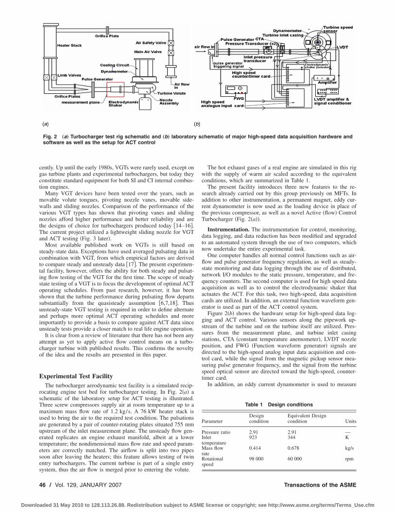
cently. Up until the early 1980s, VGTs were rarely used, except ongas turbine plants and experimental turbochargers, but today theyconstitute standard equipment for both SI and CI internal combus-tion engines.

Many VGT devices have been tested over the years, such asmovable volute tongues, pivoting nozzle vanes, movable side-walls and sliding nozzles. Comparison of the performance of thevarious VGT types has shown that pivoting vanes and slidingnozzles afford higher performance and better reliability and arethe designs of choice for turbochargers produced today �14–16�.The current project utilized a lightweight sliding nozzle for VGTand ACT testing �Fig. 3 later�.

Most available published work on VGTs is still based onsteady-state data. Exceptions have used averaged pulsating data incombination with VGT, from which empirical factors are derivedto compare steady and unsteady data �17�. The present experimen-tal facility, however, offers the ability for both steady and pulsat-ing flow testing of the VGT for the first time. The scope of steadystate testing of a VGT is to focus the development of optimal ACToperating schedules. From past research, however, it has beenshown that the turbine performance during pulsating flow departssubstantially from the quasisteady assumption �6,7,18�. Thusunsteady-state VGT testing is required in order to define alternateand perhaps more optimal ACT operating schedules and moreimportantly to provide a basis to compare against ACT data sinceunsteady tests provide a closer match to real life engine operation.

It is clear from a review of literature that there has not been anyattempt as yet to apply active flow control means on a turbo-charger turbine with published results. This confirms the noveltyof the idea and the results are presented in this paper.

Experimental Test FacilityThe turbocharger aerodynamic test facility is a simulated recip-

rocating engine test bed for turbocharger testing. In Fig. 2�a� aschematic of the laboratory setup for ACT testing is illustrated.Three screw compressors supply air at room temperature up to amaximum mass flow rate of 1.2 kg/s. A 76 kW heater stack isused to bring the air to the required test condition. The pulsationsare generated by a pair of counter-rotating plates situated 755 mmupstream of the inlet measurement plane. The unsteady flow gen-erated replicates an engine exhaust manifold, albeit at a lowertemperature; the nondimensional mass flow rate and speed param-eters are correctly matched. The airflow is split into two pipessoon after leaving the heaters; this feature allows testing of twinentry turbochargers. The current turbine is part of a single entrysystem, thus the air flow is merged prior to entering the volute.

The hot exhaust gases of a real engine are simulated in this rigwith the supply of warm air scaled according to the equivalentconditions, which are summarized in Table 1.

The present facility introduces three new features to the re-search already carried out by this group previously on MFTs. Inaddition to other instrumentation, a permanent magnet, eddy cur-rent dynamometer is now used as the loading device in place ofthe previous compressor, as well as a novel Active �flow� ControlTurbocharger �Fig. 2�a��.

Instrumentation. The instrumentation for control, monitoring,data logging, and data reduction has been modified and upgradedto an automated system through the use of two computers, whichnow undertake the entire experimental task.

One computer handles all normal control functions such as air-flow and pulse generator frequency regulation, as well as steady-state monitoring and data logging through the use of distributed,network I/O modules to the static pressure, temperature, and fre-quency counters. The second computer is used for high speed dataacquisition as well as to control the electrodynamic shaker thatactuates the ACT. For this task, two high-speed, data acquisitioncards are utilized. In addition, an external function waveform gen-erator is used as part of the ACT control system.

Figure 2�b� shows the hardware setup for high-speed data log-ging and ACT control. Various sensors along the pipework up-stream of the turbine and on the turbine itself are utilized. Pres-sures from the measurement plane, and turbine inlet casingstations, CTA �constant temperature anemometer�, LVDT nozzleposition, and FWG �Function waveform generator� signals aredirected to the high-speed analog input data acquisition and con-trol card, while the signal from the magnetic pickup sensor mea-suring pulse generator frequency, and the signal from the turbinespeed optical sensor are directed toward the high-speed, counter-timer card.

In addition, an eddy current dynamometer is used to measure

Fig. 2 „a… Turbocharger test rig schematic and „b… laboratory schematic of major high-speed data acquisition hardware andsoftware as well as the setup for ACT control

Table 1 Design conditions

ParameterDesigncondition

Equivalent Designcondition Units

Pressure ratio 2.91 2.91 —Inlettemperature

923 344 K

Mass flowrate

0.414 0.678 kg/s

Rotationalspeed

98 000 60 000 rpm



the power, from which the efficiency of turbocharger turbines canbe estimated. Because of the wide operating conditions of theturbocharger turbines, the power range requirement of the dyna-mometer is large. When engine simulations are carried out usingquasisteady methods to model the pulsating flow conditions in theengine manifold and its turbocharger, a turbine map with verywide operating conditions is required. A possible method to obtainsuch a map is by using the compressor of the turbocharger to loadthe turbine. Unfortunately, the range of data using this methodwould be insufficient given the surge and choke margins of thecompressor. An eddy current dynamometer used as the loadingdevice thus offers a much broader range of testing without theassociated aerodynamic limitations of the compressor it replaces.The dynamometer utilizes the principle of eddy-current brakingby incorporating neodymium-iron-boron magnets in a spider cre-ating a low inertia axial flux rotor.

Active Control Turbocharger

Design. The main ACT components can be seen in Figs. 3–5. Anozzleless Holset H3B turbocharger turbine was modified to ac-cept a nozzle for VGT testing. Due to the very small space avail-able and dynamic requirements, a very thin �1.5 mm thickness�section, tubular form, sliding nozzle was designed. Two embeddedattachment points at the end away from the turbine inlet casing areused to mount the nozzle on to its actuating arm �yoke� via twosmall bearing pads, which fit between the nozzle and the yoke and

assist in translating the pivoting movement of the yoke into alinear motion by the nozzle. The nozzle itself is guided toward thethroat by an inner guide, which serves both as a bearing surface tothe nozzle as well as forming the exducer section of the turbine.An outer guide houses the entire assembly and at its lower end isshaped into a bracket on which the yoke is attached and can freelypivot about. The entire assembly is held together and attached tothe face of the turbine by six 50 mm M5 bolts. The throat width tothe turbine is 26 mm wide and the nozzle can block 21.5 mm offthat passage width before reaching the stops.

The materials used for the assembly were 6082-T6 aluminiumalloy, for the entire assembly except for the nozzle, providing lightweight, with adequate strength to overcome �in the case of theyoke� fatigue, which is the major issue in this type of operation.At its most severe type of operation, the yoke achieved a safetyfactor of 10 with respect to the maximum bending stress appliedto it at its corners by the bearing pads. The nozzle was of carbonfiber reinforced plastic �CFRP� construction, providing adequatestrength for an ultralow weight against the high pressure airflowused during testing—the low nozzle weight being critical for theACT in achieving good force performance.

An electrodynamic shaker was used to drive the nozzle in theACT mode. The shaker was chosen so as to be able to provide therequired force for the limiting frequencies and amplitudes ex-pected during testing �60 Hz and approximately 20 mm, respec-tively�. Direct coupling of the shaker and nozzle was not possibledue to the nozzle being driven from the exhaust side of the tur-bine, thus forcing the shaker to be offset to the side of the exducer.The simplest way to drive the nozzle from this position was witha single-piece, pivoting yoke-type actuator arm. This makes thedesign simpler, more compact, and more importantly, allows forfar better fatigue endurance with the added advantage of signifi-cant vibration damping due to the rocker-arm type operation ofthe yoke used to drive the nozzle, which largely damps out whatwould otherwise have been severe vibrations through the turbo-charger. The total mass of all moving parts �Parts No. 2, 3, 4, 8and 9 in Fig. 3�a�� is only 0.241 kg, which was important in orderto be able to achieve the force performance required for testing,even though a penalty in terms of vibration results, since atpresent it is not possible to balance both sides of the yoke, as thetop part �nozzle� is significantly lighter to the bottom part that alsocontains approximately 0.2 kg of the moving part of the shaker.

Operation. The electrodynamic shaker is connected to thelower part of the yoke through an adjustable lever �Fig. 2� used to

Fig. 3 ACT sectional view with Mixed Flow Turbine. The thinsection nozzle can be seen protruding axially at the inlet to theturbine. The supporting guides and part of the actuator yokeare, also, shown

Fig. 4 „a… Active control turbocharger exploded view and „b…assembled turbocharger

Fig. 5 Active control turbocharger with electrodynamic shakerand dynamometer



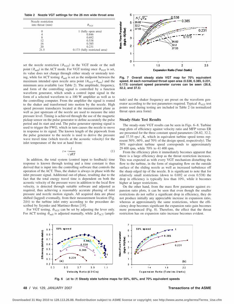
set the nozzle restriction ��VGT� in the VGT mode or the nullpoint ��null� in the ACT mode. For VGT testing once �VGT is set,its value does not change through either steady or unsteady test-ing, while for ACT testing �null is set as the midpoint between themaximum intended open nozzle area point ��VGT=�max� and theminimum area available �see Table 2�. The amplitude, frequency,and form of the controlling signal is controlled by a functionwaveform generator, which sends a control input signal in theform of a selected waveform to a 100 W amplifier as well as tothe controlling computer. From the amplifier the signal is routedto the shaker and transformed into motion by the nozzle. Highspeed pressure transducers located at the measurement plane aswell as just upstream of the nozzle are used to measure the inletpressure level. Timing is achieved through the use of the magneticpickup sensor on the pulse generator to define accurately the pulseperiod and its start and end. The pulse generator opening signal isused to trigger the FWG, which in turn causes the nozzle to movein response to its signal. The known length of the pipework fromthe pulse generator to the nozzle is used to derive the pressurewave travel time �which travels at the acoustic velocity� for theinlet temperature of the test at hand from:

t =l

��RT�1�

In addition, the total system �control input to feedback� timeresponse is known through testing and a time constant is thusderived that is input into the controlling software that controls theoperation of the ACT. Thus, the shaker is always in phase with theinlet pressure signal. Additional out-of-phase, resulting due to thefact that the total energy travel time is dependent on both theacoustic velocity of the pressure wave in addition to the local flowvelocity, is detected through suitable software and adjusted asrequired, thus achieving a reasonably accurate phasing of inletpressure and nozzle motion signals. All acquired data are phaseshifted �lagged� eventually, from their measurement location �Fig.2�b�� to the turbine inlet entry according to the procedure de-scribed by Szymko and Martinez-Botas �19�.

For VGT testing, �VGT can be set by adjusting the lever only.For ACT testing �null is adjusted manually, while ��ACT �ampli-

tude� and the shaker frequency are preset on the waveform gen-erator according to the test parameters required. Typical �VGT testpoints used during testing are included in Table 2 �in normalizedthroat open area form�:

Steady-State Test ResultsThe steady-state VGT results can be seen in Figs. 6–8. Turbine

map plots of efficiency against velocity ratio and MFP versus ERare presented for the three constant speed parameters �26.82, 32.2,and 37.55 rps/ �K, which in equivalent turbine speed terms rep-resent 50%, 60%, and 70% of the design speed, respectively�. The50% equivalent turbine speed corresponds to approximately29 400 rpm, while 70% to 41 400 rpm.

From the efficiency plots it immediately becomes apparent thatthere is a large efficiency drop as the throat restriction increases.This was expected as with every VGT mechanism disturbing theflow to the turbine, in the form of stagnating flow on the outsidesurface of the sliding nozzle as well as increased turbulence offthe sharp edged tip of the nozzle. It is significant to note that forrelatively small restrictions �down to 0.692 or even 0.538� thedrop in efficiency is typically less than 10%, while it becomeshigher at larger restrictions.

On the other hand, from the mass flow parameter against ex-pansion ratio plots, it can be seen that even though the smallerrestrictions do not suffer a significant drop in efficiency, they donot produce initially any appreciable increase in expansion ratio,whereas at approximately the same restrictions, where the effi-ciency drop becomes significant the expansion ratio gain becomesmore pronounced �Fig. 8�. Therefore, the effect that the throatrestriction has on expansion ratio increase becomes evident.

Table 2 Nozzle VGT settings for the 26 mm wide throat area

Nozzle restrictioninto throat �mm� �VGT

0 1 �fully open area�4 0.8468 0.69212 0.53816 0.38520 0.231

21.5 0.173 �fully restricted area�

Fig. 6 „a… to „f… Steady state turbine maps for 50%, 60%, and 70% equivalent speeds

Fig. 7 Overall steady state VGT map for 70% equivalentspeed. At each normalized throat open area „0.538, 0.385, 0.231,0.173… constant speed parameter curves can be seen „26.8,32.2, and 37.5…



Unfortunately, due to project constraints it was not possible tomatch an optimal MFT-oriented nozzle design to the present MFT.Instead, a straight nozzle was used with the MFT rotor as opposedto a downward inclined nozzle in the radial direction to follow theMFT leading edge angle, thus resulting in interspace diffusioneffects causing degradation of VGT performance, since the result-ing triangular interspace between the nozzle and rotor causes thisflow diffusion and therefore a decrease of the velocity component,C, hence less actual energy recovered by the turbine itself.

Active Control Turbocharger

Numerical Simulation. Our main aim of the numerical simu-lation was to demonstrate the ability of an ACT to enhance theexhaust gas energy recovery in the turbine, by comparison to aconventional VGT, since outside the optimum engine/turbocharger matching point the energy recovery capability suf-fers significantly.

A standard one-dimensional �1-D� matching calculation wasused and is based on a procedure described in the literature �8�,along with elements from the model of Chen et al. �20�, where atapered duct is considered as a simplification for a 1-D quasi-steady calculation. The main, general assumptions, therefore,made in this model involve a quasisteady approach and a highresponse actuator responding to a sine wave control input. In ad-dition, standard 1-D compressible isentropic flow equations Y �21�were applied for the derivation of the main thermodynamic pa-rameters. For a known inlet temperature, pressure, Mach numberand area, and a known exit area as modified by the nozzle, all exitparameters may be obtained by obtaining the exit Mach numberfirst.

Due to the nature of the engine-turbocharger match �volumemachine combined with a speed machine� the cycle averagedpower output of the turbocharger is less than what it could be ifthe turbine inlet pressure level �and the exhaust gas energy level ingeneral� could be raised instantaneously to its peak pressure in-stead of fluctuating substantially between atmospheric levels andits peak value. The ideal case, therefore, is for an ACT turbo-charger to virtually eliminate exhaust gas pulsation at entry to theturbine rotor so that the turbine inlet pressure at any instant oftime is equal to the peak pressure of an equivalent pulse in astandard VGT-equipped turbocharger. This, however, is not pos-sible due to limitations on the maximum nozzle displacement,efficiency drop, and the fact that at the end of the pulse period theinlet pressure levels are near atmospheric and therefore, it is notpossible to increase the inlet pressure significantly at this stage.

An example of the gain afforded by an ACT can be seen inTable 3, where a significant increase in pressure and power levelscan be seen by comparison to a conventional turbocharger �6.1%and 4.58%, respectively�. It may, also, be observed that this powerincrease comes at the expense of efficiency �a drop of 5.82%�,which was expected, but this did not have a very detrimentaleffect on the power recovered.

In addition, Fig. 9 illustrates the variation of the most importantparameters affecting ACT operation over the pulse cycle. Actualpower and pressure recovery are evident at the start and end of thepulse, while at or near the peak the effect is negligible or the sameas in VGT. Efficiency drop is proportional to the increase in pres-sure, as can be seen in Fig. 9�c�.

Operating Schedule Based on Steady-State VGT TestResults. The purpose of the steady-state VGT tests carried outwas to develop a realistic nozzle ACT schedule �in terms of nozzledisplacement amplitude and null points� for different operatingconditions �turbine speed, dynamometer load, and pulse generatorfrequency�. From Fig. 7 it may be observed that on the initial

Fig. 8 „a… Turbine expansion ratio, „b… actual power, and „c…efficiency plots with changing turbine inlet areas at 70%equivalent speed for different loads

Table 3 Conventional turbocharger comparison with ACT per-formance „max. nozzle restriction…

ParameterCycle-averaged

VGT dataEquivalent

data for ACT

Inlet pressure �bar� 1.584 1.68Mass flow rate �kg/s� 0.2531 0.1538–0.3498Turbine speed �rps� 685.9 694.2Actual Power �W� 17859 18716Isentropic Power �W� 24770 28510Cycle-averagedefficiency

0.721 0.679



steep gradient part of the MFP over ER curves, for a constantMFP �which is what quasisteadily applies to an ACT nozzle� largenozzle amplitudes are required to achieve modest inlet pressuregains. Above approximately 1.4 bar, the slope becomes signifi-cantly flatter, offering much larger gains in terms of pressure.However, at the same time there is a corresponding decrease inefficiency �Fig. 8�c��. The measure of energy availability and cor-responding actual energy recovered by the turbine is given by thefollowing equations:

Wt,is = mtCpexhT3�1 − �P03

P4�1−�exh/�exh �1��

Wt,act = �tt−sWt,is �2�

In an effort to recover more energy out of the exhaust gases,increasing the pressure drop across the turbine is one way ofachieving this aim provided, however, that the resultant efficiencydrop can be held within tolerable limits, according to Eqs. �1� and�2�. Therefore, the disparity between the FGT efficiency and theefficiency at any intermediate nozzle position ��t−s� needs to beminimal. From Fig. 6, a minimum efficiency drop occurs only atthe ends of the velocity ratio range as between 0.6 and 0.7 theFGT efficiency reaches its peak, whereas the VGT efficienciesexhibit a flatter curve thus increasing the disparity at the FGTpeak efficiency velocity ratio range.

In Fig. 8 it may be seen that only at the higher loads and in anycase only at significant throat area restrictions �below 0.5 or 50%open for the higher loads� does energy become available for in-creased recovery. At very low powers �10, 7, and even 5 mmdynamometer gaps� a high percentage of energy may be recov-ered. At 5 mm gap, some energy may be recovered but in any caseat low powers a throat area of 25% open or less is required for anysort of appreciable effect.

In addition, ACT operation is also limited by the frequency ofthe generated pulse. In Fig. 10 it may be observed that due toactuator dynamic performance the maximum amplitudes are avail-able, only at the lower frequencies �below 30 Hz�. It, therefore,becomes apparent that the most beneficial area for ACT energyextraction is at inlet pressures above 1.4 bar and at velocity ratiosbelow 0.6 �or at very high velocity ratios—above approximately0.9� and at frequencies of less than 30 Hz.

Figure 11 shows the traces of the control input signal from theFWG �activated by the pulse generator magnetic pickup sensorsignal� and the corresponding feedback signal from the LVDT fora 90° case. The system lag �mainly due to the mechanical re-sponse of the actuator� is indicated as well. For simplicity theFWG provides a sine wave to the shaker as the controlling signal.

A typical pressure waveform is not a sine wave but was con-

Fig. 9 A comparison of VGT and ACT simulation results. „a…Benefit in actual power, „b… pressure recovered, and „c… effi-ciency drop during one pulse

Fig. 10 Available nozzle amplitude performance over the testfrequency range

Fig. 11 Nozzle „LVDT position signal… lag in relation to theFWG control input waveform „35 ms lag in this case… during a50 ms pulse period „20 Hz…



sidered similar enough to a sine wave in order for the latter to beselected as the controlling waveform. The instantaneous positionof the nozzle is evaluated from:

�ACT = �ACT,min + ��ACT�1 − „sin��t�/sin��t�min…� �3�where

��ACT = �VGT − �ACT,min �4�

ACT Experimental Test Results. Experiments have so farconcentrated on investigating, primarily, the effects of the nozzlethroat area variation on pressure recovery, when the nozzle re-sponds to a sinusoidal waveform input signal. Various phasingschemes have been attempted in order to match inlet pressure andnozzle displacement traces for improved energy recovery. Unlikethe original idea to extract energy only at the lower �near ambi-ent�, energy levels of the pulse �peak-to-peak match�, where theminimum area provided by the nozzle occurs when the maximumthroat area and the peak of the pulse are in phase �i.e., the mini-mum area occurs 240° after pulse generator opening�. Three otherminimum nozzle area �maximum restriction� phase settings weretested: one, 30° after pulse generator opening, the second at 60°�at the nominal peak of the pulse�, and the third at 90° �Fig. 12�.In addition, various nozzle amplitudes, ��ACT, have been testedand comparisons against different VGT test points could be made.

Nozzle lag by comparison to the inlet pressure trace is of theorder of 100° during peak-to-peak phasing at 20 Hz. At the samefrequency when operating with the 90° out-of-phase controlscheme, the nozzle lag is of the order of 210° �see Fig. 11 and themechanical response period in crank angle terms�.

In Fig. 12, a 90° out-of-phase control scheme is illustrated. Thistype of control can be very useful as it takes advantage of thehigher energy content of the gas while the pulse generator is stillopen, as opposed to peak-to-peak phasing where energy recoveryis primarily attempted through the utilization of the low energygas stream �at near ambient levels� when the pulse generator isclosed. From this graph a clear pressure rise results �2.8% in cycleaverage terms�. This test corresponded to an area variation due tonozzle displacement of between 17.3% to 38.4% open throat area,with the VGT operating constantly at the latter figure throughoutthe fluctuations of the exhaust pulses. With reference to the dif-ferent out-of-phase control schemes tested, while at the pressurepeak the other settings have a maximum throat area, the 90° set-ting due to its phasing has less than 40% available throat area. Theconsequence of this is a higher pressure drop but a reduction inefficiency that may locally reduce the amount of power recovered.This is a well recorded tradeoff of variable inlet area turbines.However, in cycle-average terms there is a clear benefit from thistype of operation, as indicated by Table 4 for the case of 60 Hz at4 mm load in relation to the original 240° control scheme.

In low power VGT conditions where there is more restrictionfrom this device, the benefit to be gained by ACT operation is

higher than at the higher engine speed/load conditions, whereVGTs restrict the inlet to the turbine less. This is due to thesmaller efficiency drop occurring at the lower available isentropicpowers. Conversely, the turbocharger will again comparativelybenefit at the very high powers as the efficiency drop tends tofollow a constant rate that improves slightly as exemplified by theloads of 2 mm in Fig. 8�c�.

There is a discrepancy between experimental and numericalgain in inlet pressure recovery. However, direct comparisons can-not be drawn due to the fact that the two operating points aresignificantly different. Since the results illustrated concern lowpower tests, higher benefit can be expected at the higher powersetting, where there is more potential for energy recovery.

ConclusionsThe application of a VGT operation to a nozzleless FGT

equipped with a MFT rotor, requires large throat restrictions forappreciable gains in ER to be achieved, but also with significantefficiency losses too. The latter are part of the nonoptimal designmatch between the straight nozzle and the inclined MFT leadingedge causing interspace losses.

In terms of employing the turbocharger for ACT operation,there is a clear potential as confirmed by simulation results andearly ACT tests, however, this is hampered by high losses andtherefore the energy recovery is not as high as theoretically pos-sible. By focusing on certain parts of the operating envelope �lowpulse frequency operation, operation at low or very high powersand large area restrictions� the potential of the present ACT maybe demonstrated. The ACT results even for this first prototypesuggest a notable improvement in power �typically between 3%and 7%� when compared to a standard VGT operation.

NomenclatureU � blade tip speedm � mass flow rate

FGT � fixed geometry turbochargerVGT � variable geometry turbochargerACT � active control turbocharger

C � gas inlet velocityER � turbine expansion ratio or pressure ratio

P � pressureT � temperature

Cp � specific heat at constant pressureMFP � mass flow parameter, MFP= m�T0 / P0

Uinlet /Cis � velocity ratioUinlet /Cis=U3 /��2CPT01�1− �P3 / P04��−1�/��

MFT � mixed flow turbineLVDT � linear variable displacement transducerCFRP � carbon fiber reinforced plasticFWG � function waveform generator

P � pressureN � turbine rotational speed

N / �T � pseudo nondimensional speed parameter

Greek Symbols� � ratio of specific heats� � efficiency

Fig. 12 Pressure recovery achieved by an ACT compared to aVGT at 50% equivalent speed at 20 Hz „simulated exhaust gasfrequency…

Table 4 ACT energy extraction benefit over VGT at 60 Hz,4 mm load

VGTACT1240°

ACT290°

240°% Increase

90°% Increase

Wact�W�

5495 5667 5902 3.13 7.41

ER 1.55 1.69 1.74 9.18 12.57



�, �� nozzle position and position amplitude,respectively

� � angular velocity

Subscriptsis � isentropic

act � actualmin � minimum areamax � maximum area

0 � total/stagnation condition2 � pulse generator3 � turbine inlet4 � turbine exitt � turbine

t-s � total to staticnull � null position of actuator or nozzle

References�1� Ikeya, N., Yamaguchi, H., Mitsubori, K., and Kondoh, N., 1992, “Develop-

ment of Advanced Model of Turbochargher for Automotive Engines,” SAEPaper No. 920047.

�2� Tsujita, M., Niino, S., Isizuka, T., Kakinai, A., and Sato, A., 1993, “AdvancedFuel Economy in Hino New P11C Turbocharged and Charge-Cooled HeavyDuty Diesel Engine,” SAE Paper No. 930272.

�3� Minegashi, H., Matsushita, H., and Sakakida, M., 1995, “Development of aSmall Mixed-Flow Turbine for Automotive Turbochargers,” ASME Paper No.95-GT-53.

�4� Watson, N., and Janota, M. S., 1982, Turbocharging the Internal CombustionEngine, Wiley Interscience, New York.

�5� Baines, N. C., 2002, “Radial and Mixed Flow Turbines Options for High BoostTurbocharger,” 7th Int. Conference on Turbocharger and Turbocharging.

�6� Hakeem, I., 1995, “Steady and Unsteady Performance of Mixed Flow Turbinesfor Automotive Turbochargers,” Ph.D. thesis, Imperial College of Science,Technology and Medicine, London, England.

�7� Palfreyman, D., and Martinez-Botas, R. F., 2002, “Numerical Study of the

Internal Flow Field Characteristics in Mixed Flow Turbines,” ASME PaperNo. GT 2002–30372.

�8� Baines, N. C., Wallace, F. J., and Whitfield, A., 1979, “Computer Aided De-sign of Mixed-Flow Turbines for Turbochargers,” Trans. ASME: J. Eng. GasTurbines Power, 101, pp. 440–449.

�9� Abidat, M., Chen, H., Baines, N. C., and Firth, M. R., 1992, “Design of aHighly Loaded Mixed Flow Turbine,” Proc. Inst. Mech. Eng., Part A, 206, pp.95–107.

�10� Arcoumanis, C., Hakeem, I., Khezzar, L., and Martinez-Botas, R. F., 1995,“Performance of a Mixed Flow Turbocharger Turbine Under Pulsating FlowConditions,” ASME Paper No. 95-GT-210.

�11� Karamanis, N., and Martinez-Botas, R. F., 2002, “Mixed-Flow Turbines forAutomotive Turbochargers: Steady and Unsteady Performance” Int. J. EngineResearch Vol 3, No. 3, IMechE.

�12� Yamaguchi, H., Nishiyama, T., Horiai, K., and Kasuya, T., 1984, “High Per-formance Komatsu KTR150 Turbocharger,” SAE Paper No. 840019.

�13� Rodgers, C., 1990, “Review of Mixed Flow And Radial Turbine Options,”AIAA Paper 90-2414.

�14� Flaxington, D., and Szuzupak, D. T., 1982, “Variable area radial-inflow tur-bine,” 2nd Int. Conf. on Turbocharging and Turbochargers, Proc. of the IM-echE, Paper No. C36/82.

�15� Franklin, P. C., and Walsham, B. E., 1986, “Variable Geometry Turbochargersin the Field,” 3rd Int. Conf. on Turbocharging and Turbochargers, Proc. of theIMechE, Paper No. C121/86, pp. 241–250.

�16� Kawaguchi, J., Adachi, K., Kono, S., and Kawakami, T., 1999, “Developmentof VFT �Variable Flow Turbocharger�,” SAE Paper No. 1999-01-1242.

�17� Capobianco, M., and Gambarotta, A., 1992, “Variable Geometry and Waste-Gated Automotive Turbochargers: Measurements and Comparison of TurbinePerforamance,” J. Eng. Gas Turbines Power, 114, pp. 553–560.

�18� Palfreyman, D., and Martinez-Botas, R. F., 2004, “The Pulsating Flow Field ina Mixed Flow Turbine: An Experimental and Computational Study,” ASMEPaper No. GT 2004-53143.

�19� Szymko, S., and Martinez-Botas, R., 2006, “Experimental Evaluation of Tur-bocharger Turbine Performance Under Pulsating Conditions,” ASME PaperNo. GT 2005-68878.

�20� Chen, H., Hakeem, I., and Martinez-Botas, R. F., 1996, “Modelling of Turbo-charger Turbine Under Pulsating Inlet Conditions,” Proc. Inst. Mech. Eng.,Part A, 210, pp. 397–408.

�21� Yahya, S. M., 1981, “Gas Tables for Compressible Flow Calculation,” 2nd ed.,Wiley Eastern Limited, New York.



S. W. T. Spence

R. S. E. Rosborough

D. Artt

G. McCullough

School of Mechanical & Aerospace Engineering,Queen’s University Belfast,

Ashby Institute,Stranmillis Road,

Belfast BT9 5AH, UK

A Direct PerformanceComparison of Vaned andVaneless Stators for RadialTurbinesAn extensive performance investigation has been conducted on a radial turbine with threedifferent vaneless volutes and three corresponding vaned stators. Previously publishedcomparisons have been based on turbines with unmatched flow rates, meaning that theimpact of stator losses was not isolated from rotor and exit losses. Each vaned statorconfiguration tested in this investigation matched the flow rate of the correspondingvaneless volute to within 1%. The volutes and the vaned stators were all machined inorder to achieve high quality and comparable surface finishes. At all operating condi-tions, the vaneless volutes were shown to deliver a significant efficiency advantage overthe vaned stators. However, the vaneless volute turbines did not demonstrate any greatertolerance for off-design operating conditions than the vaned stator configurations. Fullperformance data are presented for the six different turbine configurations tested and aone-dimensional turbine performance model is evaluated as a means of predicting andextrapolating turbine performance. �DOI: 10.1115/1.2218518�

IntroductionA radial flow turbine is employed in almost all turbocharging

applications for its compactness, robustness, economic produc-tion, and relatively low specific speed. The radial turbine com-prises two main elements; a rotating component that extracts workfrom a swirling fluid, and a stationary component that producesthe swirl by accelerating a high pressure fluid. The stationarycomponent, referred to as the stator, can be either a series ofangled guide vanes around the periphery of the rotor or alterna-tively a vaneless housing where the flow accelerates through athroat in the tangential inlet section of the housing. In some casesboth approaches are combined where a larger vaneless housingdirects flow through a row of stator vanes into the rotor.

While there are other important roles for radial turbines, such assmall gas turbine engines, turbo-compounding, and cryogenic ex-panders, turbocharging is the most common application. For pack-aging and economic reasons, in the past practically all turbocharg-ers used a vaneless turbine stator, referred to as a volute.However, air management challenges on modern engines withhigh EGR flows have promoted the use of VGTs which combine avolute with a row of stator vanes. The stator vanes have an ad-justable element, usually a moveable vane endwall or pivotingvanes, permitting variation of the stator throat area.

Ideally a vaneless volute should provide a free vortex flow atrotor inlet with properties that are uniform around the circumfer-ence of the rotor. Bhinder �1� proposed a linear relationship be-tween A and r, where A is the cross-sectional area of the volute atany given azimuth angle and r is the radius of the centroid of thecross-sectional area at the same angle. Bhinder’s approach as-sumed incompressible flow and vaneless volutes designed on thiscriterion did not demonstrate uniformity of flow conditions aroundthe rotor circumference. Chapple et al. �2� made allowance for thecompressible nature of the flow when proposing a method fordetermining volute geometry. They also described how the analy-sis was modified to account for frictional effects by employing the

approach conventionally used to predict frictional losses in pipeflows. Turbine performance maps were presented to show im-provements in overall stage efficiency with the new volute designapproach and good accuracy in the prediction of mass flow rate atthe specified design point. The angle of the volute tongue, whichis the angle through which the flow entering the volute is turnedbefore it clears the trailing edge of the tongue, has also beenidentified as an important factor in volute design, although theoptimum values proposed by different researchers vary consider-ably �2,3�. There have been several methods proposed for predict-ing the losses incurred through the volute, all of which are basedon a mixture of fundamental fluid flow theory and empiricism�2,4,5�. A comprehensive nondimensional approach to the designof vaneless volutes has been presented by Whitfield et al. in aseries of publications �6–8� and it is not proposed to repeat thedesign methodology in any more detail in this publication.

Vaned stators for radial turbines have used guide vanes rangingfrom simple flat plates to complex cambered aerofoil shapes.Many different formats of simple 1D stator loss models have beenproposed to assist the turbine design process, although all relyheavily on empiricism and do little to help improve the existinglevel of technology. One of the more useful loss models appli-cable to vaned stators is that used by Glassman �9�, which origi-nates from work on axial flow cascades by Stewart et al. �10�.

One of the persistent difficulties with the improvement of radialturbine technology has been the lack of comprehensive publisheddata sets providing back-to-back comparisons of the effect of dif-ferent design parameters. Satisfactory comparisons cannot bemade on the basis of isolated tests on different turbines. The twomain radial turbine test programs providing extensive amounts ofcomparable test data are those undertaken by NASA, for example,�11–14� and also by Ricardo & Co., for example, �15,16�, andHiett and Johnston �17�. Bhinder �1� stated that when all otherfactors are equal, the peak efficiency of a vaneless turbine will be2–3% lower than that of a turbine with a vaned stator. However,this assertion was not supported with experimental data. Only onepublished performance comparison of vaned and vaneless statorswith the same turbine rotor has been found: Baines and Lavy �18�.The vaneless volute was cast iron while the vaned stators weremachined and therefore likely to have a much better surface finish

Contributed by the Turbomachinery Aero Division of ASME for publication in theJOURNAL OF TURBOMACHINERY. Manuscript received January 22, 2005; final manu-script received January 11, 2006. Review conducted by D. Prasad.



than the vaneless volute. The authors originally aimed to compareperformance of the vaned and vaneless stators at points ofmatched mass flow rate, although they reported that this had notbeen completely achieved in the experimental comparisons. Thevaned turbine was shown to be around 15% more efficient thanthe vaneless configuration. Internal flow investigations in thevaneless volute identified large variations in flow angle and veloc-ity around the volute exit, which the authors cited as the reasonfor poorer stage efficiency due to varying rotor incidence anglearound the circumference. While the results provided a useful in-dication, unfortunately the variation in surface finishes and thediscrepancy in the flow rates meant that the intended direct com-parison of vaned and vaneless stators had not been achieved.Rodgers �19� also states that further efficiency reductions of sev-eral percentage points occur due to the exclusion of vanednozzles.

In the present program of work the authors have sought toaddress the issue of efficient stator design through a series ofperformance tests on a turbine using the same rotor but a range ofdifferent stator configurations. This article presents a performancecomparison of vaned and vaneless stators over a range of condi-tions and at particular design points of matching mass flow rate.

Turbine DesignThree different vaneless volutes, each with a different A /r

value, were produced and tested with a radial turbine rotor. Forcomparison, three different vaned stators were designed and testedcorresponding to each of the vaneless volutes.

The turbine rotor used for the tests was a commercially avail-able rotor originating from a Holset turbocharger. In turbocharg-ers, peak turbine efficiency is often compromised for packagingconsiderations and breadth of operating range. Therefore the baseturbine rotor was reprofiled to a more “optimal” shape to giveoptimized efficiency for the test program with the philosophy thata more efficient turbine stage would more readily reveal any de-terioration in efficiency due to increased stator losses. Figure 1shows a meridional view of the turbine rotor with the basic di-mensions.

The final rotor dimensions and the primary dimensions of thevaneless volutes were determined using a one-dimensional turbineperformance prediction procedure, as detailed by Connor andFlaxington �20�. One criterion used in the 1D turbine design wasachieving an optimum value of flow incidence angle at rotor inlet,which past tests at QUB �Spence and Artt �21�� and other workershave shown to lie in the range −20 to − 40°. In this case thedesign value of incidence angle was −25±1° for all turbine con-figurations. A second design criterion was the ratio of the rotorexit relative velocity to the radial component of velocity at rotor

inlet. Rohlik �14� suggested that a moderate level of positive ac-celeration was desirable throughout the rotor blade passages andrecommended a value of 2 for this ratio. In this investigation itwas not possible to keep this value constant for each stator with-out changing the rotor geometry; however, the lowest value of thisvelocity ratio was 1.67.

Three different design operating points were fixed, covering arange of practical pressure ratios, and three corresponding vane-less volutes were specified to provide optimized performance ateach design point using the same turbine rotor. The specified de-sign operating points and the 1D stator dimensions are indicatedin Table 1. The mass flow and turbine speed values are correctedto standard turbine inlet conditions of 288 K and 101,325 Pa. Thevalue for dimensionless specific speed is a function of turbineoperating pressure and temperature; the values given in Table 1were calculated using Eq. �1� based on the proposed test rig con-

Fig. 2 Vaneless volute B

Fig. 1 Meridional view of the turbine rotor

Table 1 Summary of design point performance and 1Ddimensions

Stator A Stator B Stator C

Design point PR 1.8 2.5 3.2Design point corrected mass flowrate �kg/s�

0.249 0.245 0.228

Design point corrected speed�rev/min�

47,348 56,766 62,893

Design point U /C 0.70 0.69 0.69Dimensionless specific speed �rad� 0.90 0.89 0.89Vaneless volute throat area, A�mm2�

1703 1399 1210

Vaneless volute throat centroidradius, r �mm�

77 74 72

Vaneless volute A /r 22.1 18.9 16.8Vaned stator throat area �mm2� 1338 1189 1099Rotor exducer throat area �mm2� 2174a

Rotor inlet tip diameter �mm� 86.0Rotor inlet blade height �mm� 9.0Rotor exducer tip diameter �mm� 76.0Rotor exducer hub diameter �mm� 29.7Rotor blade number 12

aThis value of throat area was determined from a 3D model of the modified rotor.



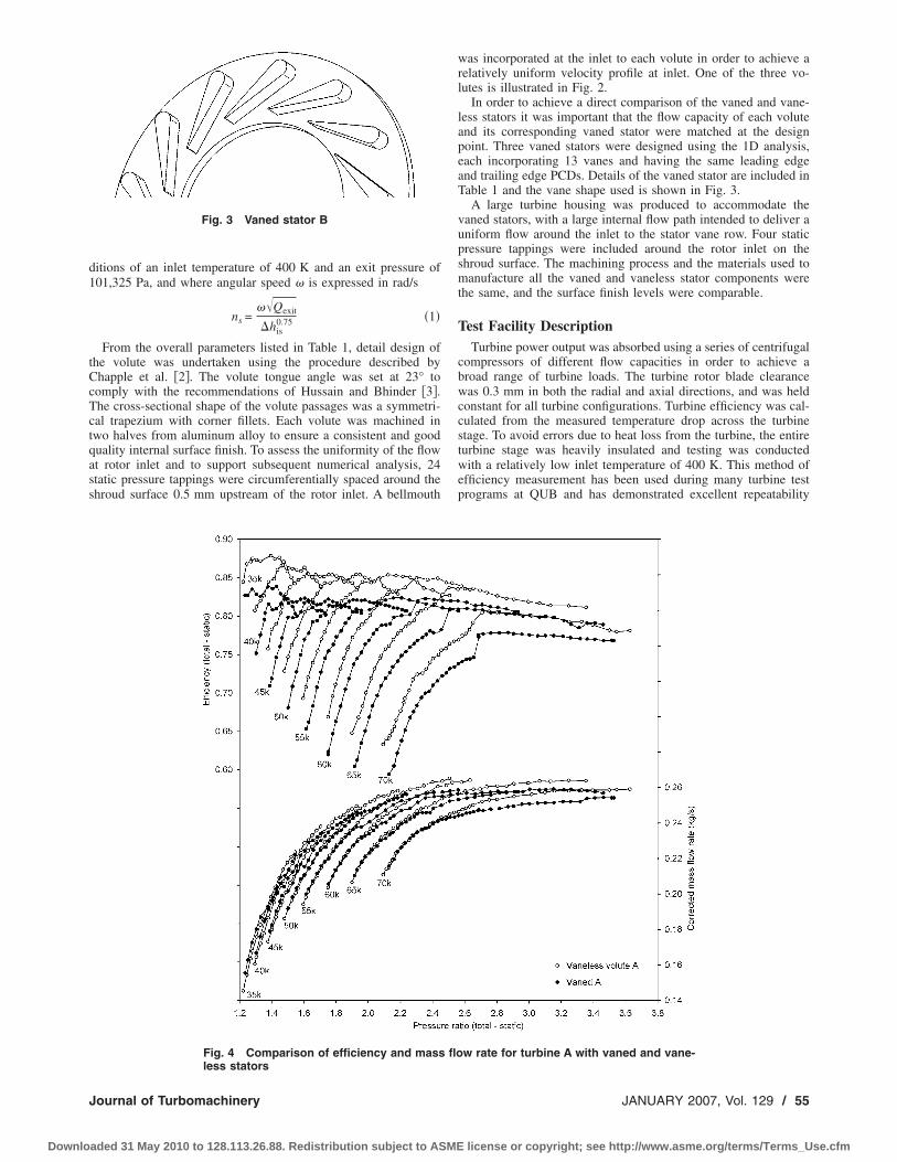
ditions of an inlet temperature of 400 K and an exit pressure of101,325 Pa, and where angular speed � is expressed in rad/s

ns =��Qexit

�his0.75 �1�

From the overall parameters listed in Table 1, detail design ofthe volute was undertaken using the procedure described byChapple et al. �2�. The volute tongue angle was set at 23° tocomply with the recommendations of Hussain and Bhinder �3�.The cross-sectional shape of the volute passages was a symmetri-cal trapezium with corner fillets. Each volute was machined intwo halves from aluminum alloy to ensure a consistent and goodquality internal surface finish. To assess the uniformity of the flowat rotor inlet and to support subsequent numerical analysis, 24static pressure tappings were circumferentially spaced around theshroud surface 0.5 mm upstream of the rotor inlet. A bellmouth

was incorporated at the inlet to each volute in order to achieve arelatively uniform velocity profile at inlet. One of the three vo-lutes is illustrated in Fig. 2.

In order to achieve a direct comparison of the vaned and vane-less stators it was important that the flow capacity of each voluteand its corresponding vaned stator were matched at the designpoint. Three vaned stators were designed using the 1D analysis,each incorporating 13 vanes and having the same leading edgeand trailing edge PCDs. Details of the vaned stator are included inTable 1 and the vane shape used is shown in Fig. 3.

A large turbine housing was produced to accommodate thevaned stators, with a large internal flow path intended to deliver auniform flow around the inlet to the stator vane row. Four staticpressure tappings were included around the rotor inlet on theshroud surface. The machining process and the materials used tomanufacture all the vaned and vaneless stator components werethe same, and the surface finish levels were comparable.

Test Facility DescriptionTurbine power output was absorbed using a series of centrifugal

compressors of different flow capacities in order to achieve abroad range of turbine loads. The turbine rotor blade clearancewas 0.3 mm in both the radial and axial directions, and was heldconstant for all turbine configurations. Turbine efficiency was cal-culated from the measured temperature drop across the turbinestage. To avoid errors due to heat loss from the turbine, the entireturbine stage was heavily insulated and testing was conductedwith a relatively low inlet temperature of 400 K. This method ofefficiency measurement has been used during many turbine testprograms at QUB and has demonstrated excellent repeatability

Fig. 3 Vaned stator B

Fig. 4 Comparison of efficiency and mass flow rate for turbine A with vaned and vane-less stators



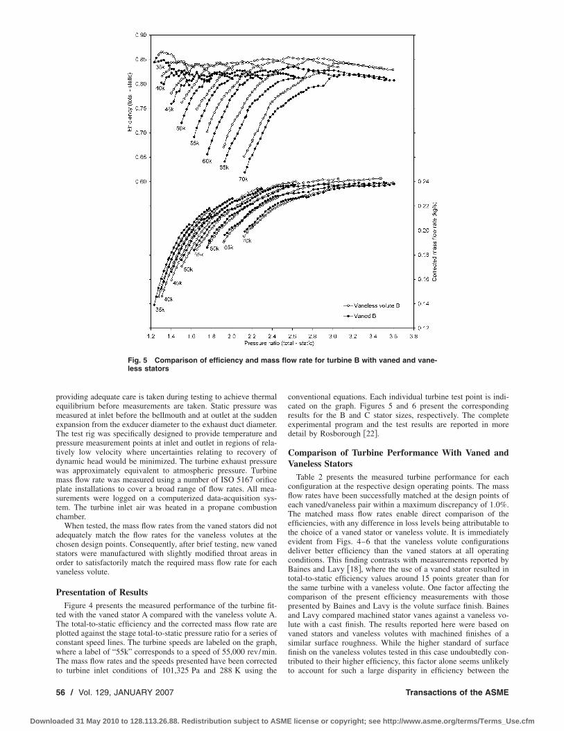
providing adequate care is taken during testing to achieve thermalequilibrium before measurements are taken. Static pressure wasmeasured at inlet before the bellmouth and at outlet at the suddenexpansion from the exducer diameter to the exhaust duct diameter.The test rig was specifically designed to provide temperature andpressure measurement points at inlet and outlet in regions of rela-tively low velocity where uncertainties relating to recovery ofdynamic head would be minimized. The turbine exhaust pressurewas approximately equivalent to atmospheric pressure. Turbinemass flow rate was measured using a number of ISO 5167 orificeplate installations to cover a broad range of flow rates. All mea-surements were logged on a computerized data-acquisition sys-tem. The turbine inlet air was heated in a propane combustionchamber.

When tested, the mass flow rates from the vaned stators did notadequately match the flow rates for the vaneless volutes at thechosen design points. Consequently, after brief testing, new vanedstators were manufactured with slightly modified throat areas inorder to satisfactorily match the required mass flow rate for eachvaneless volute.

Presentation of ResultsFigure 4 presents the measured performance of the turbine fit-

ted with the vaned stator A compared with the vaneless volute A.The total-to-static efficiency and the corrected mass flow rate areplotted against the stage total-to-static pressure ratio for a series ofconstant speed lines. The turbine speeds are labeled on the graph,where a label of “55k” corresponds to a speed of 55,000 rev/min.The mass flow rates and the speeds presented have been correctedto turbine inlet conditions of 101,325 Pa and 288 K using the

conventional equations. Each individual turbine test point is indi-cated on the graph. Figures 5 and 6 present the correspondingresults for the B and C stator sizes, respectively. The completeexperimental program and the test results are reported in moredetail by Rosborough �22�.

Comparison of Turbine Performance With Vaned andVaneless Stators

Table 2 presents the measured turbine performance for eachconfiguration at the respective design operating points. The massflow rates have been successfully matched at the design points ofeach vaned/vaneless pair within a maximum discrepancy of 1.0%.The matched mass flow rates enable direct comparison of theefficiencies, with any difference in loss levels being attributable tothe choice of a vaned stator or vaneless volute. It is immediatelyevident from Figs. 4–6 that the vaneless volute configurationsdeliver better efficiency than the vaned stators at all operatingconditions. This finding contrasts with measurements reported byBaines and Lavy �18�, where the use of a vaned stator resulted intotal-to-static efficiency values around 15 points greater than forthe same turbine with a vaneless volute. One factor affecting thecomparison of the present efficiency measurements with thosepresented by Baines and Lavy is the volute surface finish. Bainesand Lavy compared machined stator vanes against a vaneless vo-lute with a cast finish. The results reported here were based onvaned stators and vaneless volutes with machined finishes of asimilar surface roughness. While the higher standard of surfacefinish on the vaneless volutes tested in this case undoubtedly con-tributed to their higher efficiency, this factor alone seems unlikelyto account for such a large disparity in efficiency between the

Fig. 5 Comparison of efficiency and mass flow rate for turbine B with vaned and vane-less stators



present results and those of previous workers. A further consider-ation would be the uniformity of flow achieved at rotor inlet bythe vaneless volutes. It may be that a significant level of circum-ferential nonuniformity existed in the volutes used in previouswork, while the volutes used in this study achieved an improvedlevel of circumferential uniformity. It appears that a volute ofgood surface finish, achieving uniform circumferential conditions,is capable of matching or exceeding the efficiency of a vanedstator with its additional wetted surface area, secondary flows, andwakes.

Baines and Lavy also found that along with higher efficiency,the vaned stator resulted in a more sharply peaked efficiencycurve. However, Figs. 4–6 reveal that the same characteristic wasnot evident for the current comparison, in fact the shapes of theefficiency curves for the vaned and vaneless stators were verysimilar, although offset by several percentage points. As a conse-quence of the more “peaky” efficiency characteristic of the vanedstator, Baines and Lavy found the vaneless volute to be substan-tially more tolerant of off-design operating conditions at high val-ues of velocity ratio. However, Fig. 7 demonstrates that in thiscase the variation of efficiency with velocity ratio is very similarfor both the vaned stator and vaneless volute configurations ofturbine B, with neither stator option demonstrating a better toler-ance for off-design conditions over the range of turbine loadstested �0.6�U /C�0.94�. Although not presented here, the sametrend was evident for turbine configurations A and C.

Total-to-total efficiency values were calculated using a value oftotal pressure at rotor exit determined from a one-dimensionalanalysis at the exducer rms diameter. The mean relative flow ve-locity through the exducer throat area, which was calculated ateach operating point using the measured flow rate, was used inconjunction with the exducer blade angle and blade speed at therms diameter to calculate a value of absolute velocity at rotor exit.The exit total pressure was obtained from the calculated exit ve-locity and the measured exit static pressure. Total-to-total effi-ciency values at the design points of each configuration are in-cluded in Table 2. The values for the vaned stator turbinescompare well with total-to-total efficiency values presented forequivalent turbines by NASA �12,13�.

The vaneless volute is clearly the most efficient stator at all test

Fig. 6 Comparison of efficiency and mass flow rate for turbine C with vaned and vane-less stators

Table 2 Measured performance at the design point for vanedstator and vaneless volute turbines

Vanelessvolute

Vanedstator

Stator A Turbine PR 1.80 1.80Corrected speed �rev/min� 47,348 47,348Corrected mass flow rate �kg/s� 0.239 0.237Total-static efficiency �%� 85.0 81.6Total-total efficiency �%� 93.8 89.9

Stator B Turbine PR 2.50 2.50Corrected speed �rev/min� 56,766 56,766Corrected mass flow rate �kg/s� 0.237 0.236Total-static efficiency �%� 84.7 82.5Total-total efficiency �%� 93.5 91.0

Stator C Turbine PR 3.20 3.20Corrected speed �rev/min� 62,893 62,893Corrected mass flow rate �kg/s� 0.223 0.221Total-static efficiency �%� 84.7 82.9Total-total efficiency �%� 93.6 91.6



conditions, although the difference appears greatest for the turbineA configuration where the vaneless volute is around 3.5% moreefficient than the vaned stator. The difference is less for turbines Band C; around 2% for turbine C. While the design point efficiencyof the vaneless volute configuration remained relatively constantfor the three different turbine configurations, the design point ef-ficiency of the vaned stator configuration progressively increasedthrough turbines A, B, and C. Figure 8 shows the envelope of thepeak efficiency points for each of the three vaned configurations,and it is evident that better efficiencies are attainable at higherstage pressure ratios. However, at higher pressure ratios the effi-ciency achieved by the vaned C turbine is substantially better thanthe vaned A or B turbines. It might be suggested that the “C”vaned stator had a smaller throat area and consequently lowermass flow rate resulting in reduced rotor exit losses and a higherstatic efficiency. However, the differences were very similar whenthe total efficiencies were compared, so variation in exit loss doesnot appear to be the explanation. A previous publication bySpence et al. �23� highlighted the relevance of the stator/rotorthroat area ratio with regard to the maximum attainable efficiencyat a given pressure ratio. In that case best efficiency at a pressureratio of 2.2 was achieved with a stator/rotor throat area ratio of

0.5, and at a pressure ratio of 2.7 with a stator/rotor throat arearatio of 0.45. In this investigation, vaned turbine C had a stator/rotor throat area ratio of 0.5 and clearly performed better at higherpressure ratios than the other two larger vaned stators. The stator/rotor throat area ratio is implicitly linked to the turbine degree ofreaction, however, it was not possible to calculate the degree ofreaction directly from the experimental measurements since eitherthe stator loss or the stator exit static temperature was required.

The stator exit region of a small radial flow turbine is a difficultenvironment for experimental measurements and ideally a nonin-trusive method such as laser Doppler anemometry would be usedto survey the stator exit velocity and determine total pressure.Such measurements were not available in this investigation andconsequently absolute measurements of the losses through thevaned and vaneless stators cannot be obtained. However, the dif-ference in incurred losses between the vaned and vaneless statorswas determined with confidence from the experimental measure-ments. Figure 9 shows the additional loss incurred by the vanedstator relative to the vaneless volute at the design point for each ofthe three turbine configurations. The difference in vaned and vane-less stator loss is very similar for each turbine; although thesevalues do vary with changing turbine operating conditions. The

Fig. 7 Comparison of efficiency for vaned stator B and vane-less volute B, plotted against velocity ratio U /C

Fig. 8 Peak efficiency envelopes for the vaned stator configurations A, B, and C

Fig. 9 Difference in vaned and vaneless stator losses for eachof the turbine configurations A, B, and C



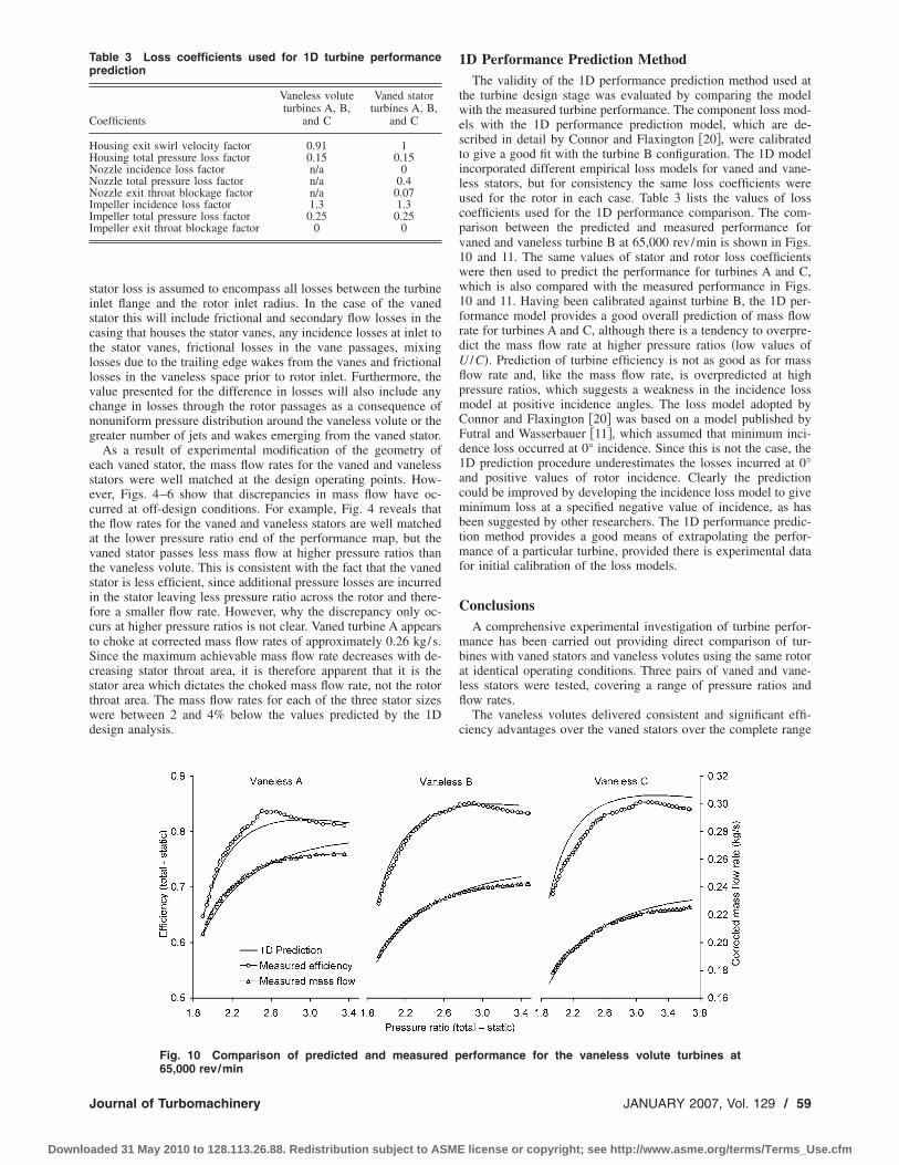
stator loss is assumed to encompass all losses between the turbineinlet flange and the rotor inlet radius. In the case of the vanedstator this will include frictional and secondary flow losses in thecasing that houses the stator vanes, any incidence losses at inlet tothe stator vanes, frictional losses in the vane passages, mixinglosses due to the trailing edge wakes from the vanes and frictionallosses in the vaneless space prior to rotor inlet. Furthermore, thevalue presented for the difference in losses will also include anychange in losses through the rotor passages as a consequence ofnonuniform pressure distribution around the vaneless volute or thegreater number of jets and wakes emerging from the vaned stator.

As a result of experimental modification of the geometry ofeach vaned stator, the mass flow rates for the vaned and vanelessstators were well matched at the design operating points. How-ever, Figs. 4–6 show that discrepancies in mass flow have oc-curred at off-design conditions. For example, Fig. 4 reveals thatthe flow rates for the vaned and vaneless stators are well matchedat the lower pressure ratio end of the performance map, but thevaned stator passes less mass flow at higher pressure ratios thanthe vaneless volute. This is consistent with the fact that the vanedstator is less efficient, since additional pressure losses are incurredin the stator leaving less pressure ratio across the rotor and there-fore a smaller flow rate. However, why the discrepancy only oc-curs at higher pressure ratios is not clear. Vaned turbine A appearsto choke at corrected mass flow rates of approximately 0.26 kg/s.Since the maximum achievable mass flow rate decreases with de-creasing stator throat area, it is therefore apparent that it is thestator area which dictates the choked mass flow rate, not the rotorthroat area. The mass flow rates for each of the three stator sizeswere between 2 and 4% below the values predicted by the 1Ddesign analysis.

1D Performance Prediction MethodThe validity of the 1D performance prediction method used at

the turbine design stage was evaluated by comparing the modelwith the measured turbine performance. The component loss mod-els with the 1D performance prediction model, which are de-scribed in detail by Connor and Flaxington �20�, were calibratedto give a good fit with the turbine B configuration. The 1D modelincorporated different empirical loss models for vaned and vane-less stators, but for consistency the same loss coefficients wereused for the rotor in each case. Table 3 lists the values of losscoefficients used for the 1D performance comparison. The com-parison between the predicted and measured performance forvaned and vaneless turbine B at 65,000 rev/min is shown in Figs.10 and 11. The same values of stator and rotor loss coefficientswere then used to predict the performance for turbines A and C,which is also compared with the measured performance in Figs.10 and 11. Having been calibrated against turbine B, the 1D per-formance model provides a good overall prediction of mass flowrate for turbines A and C, although there is a tendency to overpre-dict the mass flow rate at higher pressure ratios �low values ofU /C�. Prediction of turbine efficiency is not as good as for massflow rate and, like the mass flow rate, is overpredicted at highpressure ratios, which suggests a weakness in the incidence lossmodel at positive incidence angles. The loss model adopted byConnor and Flaxington �20� was based on a model published byFutral and Wasserbauer �11�, which assumed that minimum inci-dence loss occurred at 0° incidence. Since this is not the case, the1D prediction procedure underestimates the losses incurred at 0°and positive values of rotor incidence. Clearly the predictioncould be improved by developing the incidence loss model to giveminimum loss at a specified negative value of incidence, as hasbeen suggested by other researchers. The 1D performance predic-tion method provides a good means of extrapolating the perfor-mance of a particular turbine, provided there is experimental datafor initial calibration of the loss models.

ConclusionsA comprehensive experimental investigation of turbine perfor-

mance has been carried out providing direct comparison of tur-bines with vaned stators and vaneless volutes using the same rotorat identical operating conditions. Three pairs of vaned and vane-less stators were tested, covering a range of pressure ratios andflow rates.

The vaneless volutes delivered consistent and significant effi-ciency advantages over the vaned stators over the complete range

Table 3 Loss coefficients used for 1D turbine performanceprediction

Coefficients

Vaneless voluteturbines A, B,

and C

Vaned statorturbines A, B,

and C

Housing exit swirl velocity factor 0.91 1Housing total pressure loss factor 0.15 0.15Nozzle incidence loss factor n/a 0Nozzle total pressure loss factor n/a 0.4Nozzle exit throat blockage factor n/a 0.07Impeller incidence loss factor 1.3 1.3Impeller total pressure loss factor 0.25 0.25Impeller exit throat blockage factor 0 0

Fig. 10 Comparison of predicted and measured performance for the vaneless volute turbines at65,000 rev/min



of pressure ratios tested. At the design operating conditions, theefficiency advantage was between 2% and 3.5%. Previous com-parisons have typically compared machined stator vanes with avaneless volute having a rough cast surface finish with a highlevel of roughness, and found the volute to be less efficient. Whilethese are not strictly comparable situations, the implication is thathousing surface roughness is a significant factor in overall turbineefficiency. The turbines configured with vaneless volutes, whilemaintaining an efficiency advantage, were not found to be anymore tolerant of off-design operating conditions than the vanedstator turbines.

The best achievable efficiency at a given turbine pressure ratiowith a vaned stator was a function of the stator to rotor throat arearatio, with a smaller ratio giving better efficiency at higher pres-sure ratios. A ratio equal to 0.5 gave good efficiency at moderatepressure ratios.

A volute design method presented by Chapple et al. was usedand yielded good turbine efficiency levels and mass flow rateswithin 4% of the design values. A 1D turbine design predictionmethod presented by Connor and Flaxington was used for theturbine design and was subsequently shown to be a good methodof extrapolating turbine performance providing experimental datawere available to calibrate the loss coefficients in the model.

AcknowledgmentThe authors would like to acknowledge the financial support of

EPSRC �Grant No. GR/M41865�, without which this investigationwould not have been possible. Thanks are also due to Holset En-gineering Co. Ltd. for ongoing technical and hardware support,and particularly to Nick Sharp for his interest, enthusiasm, andgenerosity with his time.

NomenclatureVGT � variable geometry turbineEGR � exhaust gas recirculation

1D � one dimensionalU /C � turbine blade speed velocity ratioPCD � pitch circle diameterrms � root mean square

ns � dimensionless specific speed �rad�Qexit � volumetric flow rate at rotor exit �m3/s��his � isentropic stage enthalpy drop �J/kg�

� � angular speed �rad/s�

References�1� Bhinder, F. S., 1969, “Investigation of Flow in the Nozzle-Less Spiral Casing

of a Radial Inward-Flow Gas Turbine,” Proc. Inst. Mech. Eng., 184, pp. 66–71.

�2� Chapple, P. M., Flynn, P. F., and Mulloy, J. M., 1980, “Aerodynamic Design ofFixed and Variable Geometry Nozzleless Turbine Casings,” Trans. ASME: J.Eng. Gas Turbines Power, 102, pp. 141–147.

�3� Hussain, M., and Bhinder, F. S., 1984, “Experimental Study of The Perfor-mance of a Nozzleless Volute Casing for Turbocharger Turbines,” SAE PaperNo. 840571.

�4� Kastner, L. J., and Bhinder, F. S., 1975, “A Method for Predicting the Perfor-mance of a Centripetal Gas Turbine Fitted With a Nozzle-less Volute Casing,”ASME Paper No. 75-GT-65.

�5� Chen, H., 1996, “Design Methods of Volute Casings for Turbocharger TurbineApplications,” Proc. Inst. Mech. Eng., Part A, 210, pp. 149–156.

�6� Whitfield, A., and Mohd Noor, A. B., 1994, “Design and Performance ofVaneless Volutes for Radial Inflow Turbines. 1. Non-dimensional ConceptualDesign Considerations,” Proc. Inst. Mech. Eng., Part A, 208, pp. 199–211.

�7� Whitfield, A., MacGregor, S. A., and Mohd Noor, A. B., 1994, “Design andPerformance of Vaneless Volutes for Radial Inflow Turbines. 2. ExperimentalInvestigation of the Mean Line Performance-Assessment of Empirical DesignParameters,” Proc. Inst. Mech. Eng., Part A, 208, pp. 213–224.

�8� MacGregor, S. A., Whitfield, A., and Mohd Noor, A. B., 1994, “Design andPerformance of Vaneless Volutes for Radial Inflow Turbines. 3. ExperimentalInvestigation of the Internal Flow Structure,” Proc. Inst. Mech. Eng., Part A,208, pp. 295–302.

�9� Glassman, A. T., 1976, “Computer Program for Design and Analysis of RadialInflow Turbines,” NASA/TN D-8164.

�10� Stewart, W. L., Whitney, W. J., and Wong, R. Y., 1960, “A Study of BoundaryLayer Characteristics of Turbomachine Blade Rows and Their Relation toOverall Blade Loss,” J. Basic Eng., 82�3�, pp. 588–592.

�11� Futural, S. M., and Wasserbauer, C. A., 1965, “Off-Design Performance Pre-diction With Experimental Verification for a Radial-Inflow Turbine,” NASA,TN/D-2621.

�12� Kofskey, M. G., and Nusbaum, W. J., 1972, “Effects of Specific Speed onExperimental Performance of a Radial-Inflow Turbine,” NASA, TN/D-6605.

�13� Kofskey, M. G., and Wasserbauer, C. A., 1966, “Experimental PerformanceEvaluation of a Radial-Inflow Turbine Over a Range of Specific Speeds,”NASA, TN/D-3742.

�14� Rohlik, H. E., 1968, “Analytical Determination of Radial-Inflow Turbine De-sign Geometry for Maximum Efficiency,” NASA TN/D-4384.

�15� Palmer, R. M., 1956, “D.I.G.T. Radial Inflow Turbine-Scroll and NozzlePerformance—Part II,” Ricardo Internal Report No. 1368, Ricardo & Co.,Sussex.

�16� Hiett, G. F., 1959, “D.I.G.T. Radial Inflow Turbine-Cold Tests on Turbine B,Turbine A and Turbine D,” Ricardo Internal Report No. 1412, Ricardo & Co.,Sussex.

�17� Hiett, G. F., and Johnston, I. H., 1963, “Experiments Concerning the Aerody-namic Performance of Inward Flow Radial Turbines,” Proc. Inst. Mech. Eng.,178, pp. 28–42.

�18� Baines, N. C., and Lavy, M., 1990, “Flows in Vaned and Vaneless Stators ofRadial Inflow Turbocharger Turbines,” Institution of Mechanical EngineersTurbochargers and Turbocharging Conference, Paper No. C405/005, pp. 7–12.

Fig. 11 Comparison of predicted and measured performance for the vaned stator turbines at65,000 rev/min



�19� Rodgers, C., 2000, “Radial Turbines-Blade Number and Reaction Effects,”ASME Paper No. 2000-GT-456.

�20� Connor, W. A., and Flaxington, D., 1994, “A One-Dimensional PerformancePrediction Method for Radial Inflow Turbines,” Institution of Mechanical En-gineers Turbochargers and Turbocharging Conference, Paper No. C484/041/94, pp. 271–282.

�21� Spence, S. W. T., and Artt, D. W., 1998, “An Experimental Assessment ofIncidence Losses in a Radial Inflow Turbine Rotor,” Proc. Inst. Mech. Eng.,

Part A, 212, pp. 43–53.�22� Rosborough, R. S. E., 2003, “An Experimental Assessment of Different Vaned

and Vaneless Stators for a Radial Inflow Turbine,” Ph.D. thesis, Queen’s Uni-versity of Belfast, UK.

�23� Spence, S. W. T., Doran, W. J., and Artt, D. W., 1999, “Experimental Perfor-mance Evaluation of a 99.0 mm Radial Inflow Nozzled Turbine at LargerStator/Rotor Throat Area Ratios,” Proc. Inst. Mech. Eng., Part A, 213, pp.205–218.



Bo Song1

Wing F. Ng

Mechanical Engineering Department,Virginia Polytechnic Institute

and State University,Blacksburg, VA 24061

Joseph A. Cotroneo

Douglas C. Hofer

GE Energy,1 River Road,

Schenectady, NY 12345

Gunnar SidenGE Energy,

300 Garlington Road,Greenville, SC 29602

Aerodynamic Design and Testingof Three Low Solidity SteamTurbine Nozzle CascadesThree sets of low solidity steam turbine nozzle cascades were designed and tested. Theobjective was to reduce cost through a reduction in parts count while maintaining orimproving performance. The primary application is for steam turbine high pressure sec-tions where Mach numbers are subsonic and high levels of unguided turning can betolerated. The base line design A has a ratio of pitch to axial chord of 1.2. This is thepitch diameter section of a 50% reaction stage that has been verified by multistage testingon steam to have a high level of efficiency. Designs B and C have ratios of pitch to axialchord of 1.5 and 1.8, respectively. All three designs satisfy the same inlet and exit vectordiagrams. Analytical surface Mach number distributions and boundary layer transitionpredictions are presented. Extensive cascade test measurements were carried out for abroad incidence range from −60 to +35 deg. At each incidence, four outlet Mach num-bers were tested, ranging from 0.2 to 0.8, with the corresponding Reynolds numbervariation from 1.8�105 to 9.0�105. Experimental results of loss coefficient and bladesurface Mach number are presented and compared for the three cascades. The experi-mental results have demonstrated low losses over the tested Mach number range for awide range of incidence from −45 to 15 deg. Designs B and C have lower profile lossesthan design A. The associated flow physics is interpreted using the results of wake profile,blade surface Mach number distribution, and blade surface oil flow visualization, withthe emphasis placed on the loss mechanisms for different flow conditions and the lossreduction mechanism with lower solidity. The effect of the higher profile loading of thelower solidity designs on increased end wall losses induced by increased secondary flow,especially on low aspect ratio designs, is the subject of ongoing studies.�DOI: 10.1115/1.2372774�

Introduction

Low solidity airfoil designs offer advantages to steam turbinesused in the power generation industry. The most obvious is re-duced parts count and therefore reduced cost. Alternatively, axialchord can be reduced resulting in a shorter turbine, which is usefulin tradeoffs between rotor dynamics and turbine efficiency. Effi-ciency is also of paramount importance so these low solidity de-signs must not compromise performance. In combined cycle highpressure steam turbines the blades can be small but there are mini-mum manufacturing and reliability limits on trailing edge thick-ness. A large ratio of trailing edge thickness to throat will lowerturbine efficiency. Low solidity airfoils reduce these trailing edgeblockage losses. Conversely, lower solidity airfoils for the sameduty are more highly loaded than their higher solidity counter-parts. The objective of this work is to define airfoils that have lowprofile losses at low solidity and to determine what levels of lowsolidity are attainable with high efficiency. The optimum solidityshould be a good trade off for weight and efficiency �1,2�. Anotherissue to consider is that more highly loaded airfoils can tend tohave higher endwall losses generated by increased secondary flow�3,4�. This can be a significant source of efficiency loss for lowaspect ratio designs. The profile losses of the low solidity designspresented here are actually lower than the base line higher soliditydesign. This will help counter the increased end wall losses. The

effect of low solidity designs on secondary flow in the endwallregion and associated losses is the subject of ongoing studies.

Prior work on low solidity or the so-called high lift turbineblading has been carried out mostly on gas turbine low-pressureturbines, which operate at relatively low Reynolds number �up to21,000�. Solomon �5,6� found the efficiency gain by reduced so-lidity on a low-pressure turbine was conditional, jointly dependenton inlet turbulence, Reynolds number, and clocking effect. Howellet al. �7� further reduced solidity of high lift blading �datum pro-file� based on understanding of the boundary layer behavior. Theyachieved 15% greater lift under unsteady flow condition, with thenew reduced-solidity profile losses only slightly higher than thoseof the datum profile. They referred to this new blading as “ultra-high lift” �UHL� concept. However, with steady inflow, theyfound the UHL profiles performed poorly. The following full-scale LP turbine rig test showed lower efficiencies associated withthe afore-mentioned UHL blading than the datum �8�. Anothereffort by Howell et al. �9� detailed a study into the unsteadyboundary layer behavior in two high lift and one ultrahigh lift LPturbines, showing advantage of the low solidity concept in LPturbines under unsteady flow and stage interaction. These priorstudies have shown that the high lift turbines benefit from un-steady effects of upstream blade wakes, with a comprehensivesummary given by Hodson �10�. The parametric effect of reducedsolidity on profile losses seems not to be so certain from thesestudies.

The work by Gonzalez et al. �11� contributed to high lift LPturbine blading research with low-speed cascade steady and un-steady experiments. Their work demonstrated 10% profile lossreduction by redesigning pressure and suction surfaces to makethicker profiles. The cascade testing was performed with relativelylow Reynolds numbers up to 30,000. Their results also support animportant idea of an optimum axial position for the peak Mach

1Currently Sr. Product Development Engineer with Gardner Denver, Inc.Contributed by the International Gas Turbine Institute �IGTI� of ASME for pub-

lication in the JOURNAL OF TURBOMACHINERY. Manuscript received October 1, 2003;final manuscript received March 1, 2004. IGTI Review Chair: A. J. Strazisar. Paperpresented at the International Gas Turbine and Aeroengine Congress and Exhibition,Vienna, Austria, June 13–17, 2004, Paper No. 2004-GT-53329.



number, or put it another way, the concept of aft loading to reducelosses is not absolute �this point is supported by the current workas will be shown in the paper�. Low speed wind tunnel testing ofa high lift LP turbine cascade by Houtermans et al. �12� providedmore profile loss data to the open literature over an incidencerange from −9 to 5 deg at Reynolds numbers of 50,000 to200,000. The blade used was a front-loaded type with the peakvelocity at 32% of the suction side length. This research alsoindicated the position of the peak velocity coupled with the inci-dence had a strong effect on the cascade performance. Cascadetesting of three HP turbine blades �front loaded, midloaded, aftloaded� at relatively high Reynolds numbers �30,000–100,000� byCorriveau and Sjolander �13� also indicated important influence ofloading distribution on the cascade performance and the depen-dence of performance gain on conditions. The effect of loadingdistribution on turbine blade performance was studied earlier, andagain, the conclusion to favor front or aft loading is somewhat incontradiction �14–16�.

The particular airfoil design addressed here is the pitch linesection of a master nozzle design used in 50% reaction high pres-sure steam turbines for the combined cycle power generation mar-ket. The base line design A has been applied in the high pressuresections of GE’s new 107FA and 109FB HEAT™ steam turbines�17,18�. Laboratory testing of a 12 stage prototype on steam hasdemonstrated a high level of efficiency. The next design objectiveis a reduced cost product that maintains this high efficiency level.Reduced solidity airfoil design optimization is one part of thateffort. The design and test of the base line plus two 2D cascadeswith decreased solidity will be presented here. It should be notedthat the current design for steam turbine application rendered ahigh Reynolds number �2�106� and the testing was extended toas wide a range of conditions as possible for sufficient experimen-tal demonstration �incidence: −60 to +35 deg, outlet Mach num-ber: 0.2–0.8, and Reynolds number: 1.8�105–9.0�105�. Theblade profiles of the reduced-solidity cascades were optimized forperformance improvement. Therefore, the current work should bealso of general interest with an addition of data and reference toturbine blading research with respect to effects of solidity, profile,and loading distribution.

Cascade Design/OptimizationThe airfoils were designed using an in house Bezier curve blade

geometry generator to allow for maximum flexibility in optimiz-ing the profile shape. Flow analysis was performed with a 2DEuler flow solver with boundary layer and loss calculations �19�.This level of analysis is believed to be proper for designing air-foils for 2D cascade testing. It gives the advantage of quick turnaround time allowing for a maximum number of design iterations.All three cascades were designed for the same duty. The designReynolds number is approximately 2�106. Figure 1 gives theprofile shapes of designs A, B, and C. The cascade nomenclatureused in this study is illustrated in Fig. 2. Table 1 gives a summaryof some relevant design parameters. The base line design A has aratio of pitch to axial chord of 1.2 while for designs B and C thevalues are 1.5 and 1.8, respectively. Design A has a solidity of1.22 while for designs B and C the values are 1.06 and 0.93,respectively.

Variations in stagger and unguided turning were investigated aspart of the profile optimization process. As expected, reduced so-lidity leads to higher unguided turning and more tangential stag-ger. The higher stagger is needed to form good throat convergingpassage geometry. High unguided turning can be detrimental athigher Mach numbers because of increased shock losses but is notnecessarily a problem at the subsonic Mach numbers of thesedesigns. Decreased solidity causes increased loading and can leadto high diffusion on the suction surface downstream of the throat.This high diffusion can lead to increased boundary layer thicknessand even flow separation. The philosophy taken here was to movesome of the load forward on the lower solidity designs to controlsuction side diffusion and hence limit losses. It should be notedthat even though some of the load was moved forward, the distri-butions are still closer to aft loaded than uniformly loaded. Pres-sure and suction surface Mach number distributions over a rangeof exit Mach numbers are shown in Fig. 3 for all three designs.

Reynolds numbers at nozzle exits for the 107FA high pressureturbine range from about 2�106 in the back end to about 5�106 in the front end. The Reynolds numbers for this cascadetesting are lower due to rig pressure limitations and cover a range

Fig. 1 Cascade profile shapes



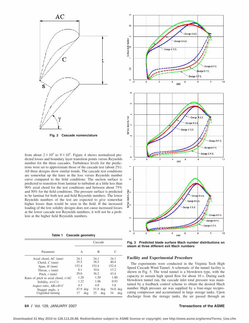
from about 2�105 to 9�105. Figure 4 shows normalized pre-dicted losses and boundary layer transition points versus Reynoldsnumber for the three cascades. Turbulence levels for the predic-tions were set to approximate those of the cascade test �about 2%�.All three designs show similar trends. The cascade test conditionsare somewhat up the knee in the loss versus Reynolds numbercurve compared to the field conditions. The suction surface ispredicted to transition from laminar to turbulent at a little less than90% axial chord for the test conditions and between about 75%and 50% for the field conditions. The pressure surface is predictedto be laminar for both test and field Reynolds numbers. The lowerReynolds numbers of the test are expected to give somewhathigher losses than would be seen in the field. If the increasedloading of the low solidity designs does not cause increased lossesat the lower cascade test Reynolds numbers, it will not be a prob-lem at the higher field Reynolds numbers.

Facility and Experimental ProcedureThe experiments were conducted in the Virginia Tech High

Speed Cascade Wind Tunnel. A schematic of the tunnel facility isshown in Fig. 5. The wind tunnel is a blowdown type, with thecapacity to sustain high speed flow for about 10 s. During eachblowdown tunnel run, the cascade inlet total pressure was main-tained by a feedback control scheme to obtain the desired Machnumber. High pressure air was supplied by a four-stage recipro-cating compressor and accumulated in large storage tanks. Upondischarge from the storage tanks, the air passed through an

Fig. 2 Cascade nomenclature

Table 1 Cascade geometry

Parameter

Cascade

A B C

Axial chord, AC �mm� 24.1 24.1 24.1Chord, C �mm� 35.5 38.5 40.4Span, H �mm� 152.4 152.4 152.4Throat, s �mm� 8.1 10.6 13.2Pitch, t �mm� 29.0 36.2 43.4

Ratio of pitch to axial chord, t /AC 1.20 1.50 1.80Solidity, �=C / t 1.22 1.06 0.93

Aspect ratio, AR=H /C 4.3 4.0 3.8Stagger angle, � 47.9 deg 51.9 deg 54.0 degUnguided turning 17 deg 25 deg 34 deg

Fig. 3 Predicted blade surface Mach number distributions onsteam at three different exit Mach numbers



activated-aluminum dryer for dehumidification and then pro-ceeded through the settling chamber where a flow straightener anda screen were placed to make the flow uniform. Upstream of thetest section, a turbulence grid was inserted to increase inlet free-stream turbulence to a level of about 2%. After passing throughthe test section, the flow was guided into the exhaust pipe, andfinally discharged to the atmosphere.

The test section is better shown by an insert view in Fig. 5 anda sideview picture in Fig. 6. The cross section of the cascade inlethad dimensions of 232 mm�152 mm �height�width�. Thetested cascade was mounted between a pair of Plexiglas sidewalls,

which allow for visual observation and optical measurements. Thesidewalls fit into the circular window. By rotating the sidewall-cascade assembly, different incidence angles could be obtained forthe tests. The cascade flow uniformity/periodicity was achieved byusing no less than six blades and employing a pair of tailboardsdownstream of the cascade along with an adjustable bottom wallat the inlet. The number of blades mounted to construct the cas-cade depended on the available space in the test section, whichwas a function of the cascade solidity and different incidenceangles. It turned out that 8–10 blades were used for design A, and7–8 blades for design B, and six blades for design C. The tail-boards were set parallel to the cascade design outlet flow angle.For different incidence angles, the axial length of the adjustablebottom wall was set to fit the cascade very well. Figure 6 showsone example of a negative incidence test case.

Temperature in the tunnel was measured using a type K ther-mocouple total temperature probe located upstream of the testsection. The facility operated with an inlet total temperature rangeof 277–298 K in the current experiment. Aerodynamic measure-ments are illustrated in Fig. 7. All the aerodynamic measurementswere performed in the midspan for a wide range of outlet Machnumbers from 0.21 to 0.80. Since the tunnel cannot control Machnumber and Reynolds number independently, the correspondingReynolds number varied from 1.8�105 to 9.0�105. Broad inci-dence ranges �from −45 to 30 deg for designs A and C and from−60 to 35 deg for design B� were tested for each outlet Machnumber.

Inlet total pressure was measured one axial chord upstream ofthe cascade in the spanwise center of the middle passage using atotal pressure probe. The facility operated with an inlet total pres-sure range of 0.97–1.81�105 Pa in the current experiment. Inletflow angle was checked by traversing a three-hole angle probe100% axial chord upstream of the cascade for selected Mach num-bers and incidence angles. It was found the inlet flow was parallel

Fig. 4 Predicted losses and boundary layer transition pointson steam at constant Mach number

Fig. 5 Virginia Tech High Speed Cascade Wind Tunnel

Fig. 6 Cascade test section

Fig. 7 Aerodynamic measurements



to the top and bottom walls of the test section to within 0.5 degdeviation. Thirteen sidewall pressure taps were aligned in thepitchwise direction 100% axial chord upstream of the cascade,covering the middle three passages. The static pressures measuredby these taps were used to monitor the inlet flow uniformity. Thestatic pressures taken in the middle passage were averaged andused along with the measured total pressure to determine the inletMach number. At the cascade outlet, a three-hole angle probe wastraversed 42% of the axial chord downstream of the blade trailingedge to measure outlet total pressure, Mach number, and flowangle. The traverse range covered the middle three passages pro-viding good monitoring of the outlet flow periodicity. Overallaerodynamic parameters at the outlet were averaged for one pitch.This pitch was chosen such that the wake profile of the middleblade was completely included. The two blades that composed themiddle passage were instrumented on the pressure surface andsuction surface respectively for blade surface pressure measure-ment. Blade surface oil flow visualization was performed on themiddle four blades for selected test cases to help understandingthe flow.

Throughout the experiments, uncertainty was introduced fromdifferent sources including instrumentation, flow aperiodicity, andtunnel unsteadiness �although the latter two were relatively small�.The overall uncertainty for the major measured flow quantitieswas estimated to have the following range: Mach number within±5%, loss coefficient within ±5%.

Results Discussion

Flow Uniformity and Periodicity. In cascade testing, pitch-wise flow uniformity/periodicity is an important requirement.Both inlet and outlet aerodynamic measurements in the currentexperiments showed good inlet flow uniformity and outlet flowperiodicity. A representative example of the experimental resultsis shown in Fig. 8. The inlet flow uniformity is represented byinlet static pressure coefficient Cp1 �normalized by the inlet totalpressure�. The outlet flow periodicity is represented by wake pro-file �quantified by local loss coefficient, normalized Y�.

In 2D linear cascade testing, another important concern is thespanwise flow uniformity �3D effect from the sidewall�. In turbinecascade testing, previous experience has shown that solid side-walls are adequate, particularly for high aspect ratio cascades suchas the ones used in this study. Sieverding �20� recommended mini-mum aspect ratios to obtain reliable 2D midspan performance data

in turbine cascade tests from 1.6 to 2.2 based on different velocityratios across the cascade. In the current tests aspect ratios greaterthan 3.8 were used ensuring good spanwise flow uniformity. Con-firmation of the spanwise flow uniformity is provided by bladesurface oil flow visualization. One example is shown in Fig. 9.The picture was taken after the tunnel run and the flow was visu-alized through the oil pattern left on the blade surface. In additionto showing good spanwise flow uniformity, pitchwise periodicflow was also indicated by blade surface flow visualization �seeFig. 9 for good repeatability of the oil pattern from blade toblade�.

Profile Losses. The profile losses of the three cascades weretested at incidence angles of −45, −30, 0, 15, and 30 deg. At eachincidence, four Mach numbers ranging from 0.21 to 0.8 weretested. The overall aerodynamic parameters for the outlet flowwere averaged from the measured pitchwise local quantities usinga mixing algorithm. The algorithm calculated a mixing processwith the conservation of mass and momentum, through which thecascade outlet flow turned to a uniform flow. The obtained uni-form total and static pressure �Pt2m

and Ps2m� were then used to

calculate the loss coefficient Ym.Figure 10 shows the experimental results of the loss develop-

ment with outlet Mach number at three representative incidenceangles: −45, 0, and 30 deg, respectively. The corresponding varia-tion of Reynolds number with M2 is also plotted in the chart. As

Fig. 8 Pitchwise flow uniformity and periodicity

Fig. 9 Flow uniformity and periodicity confirmed by blade sur-face flow visualization „S.S.…



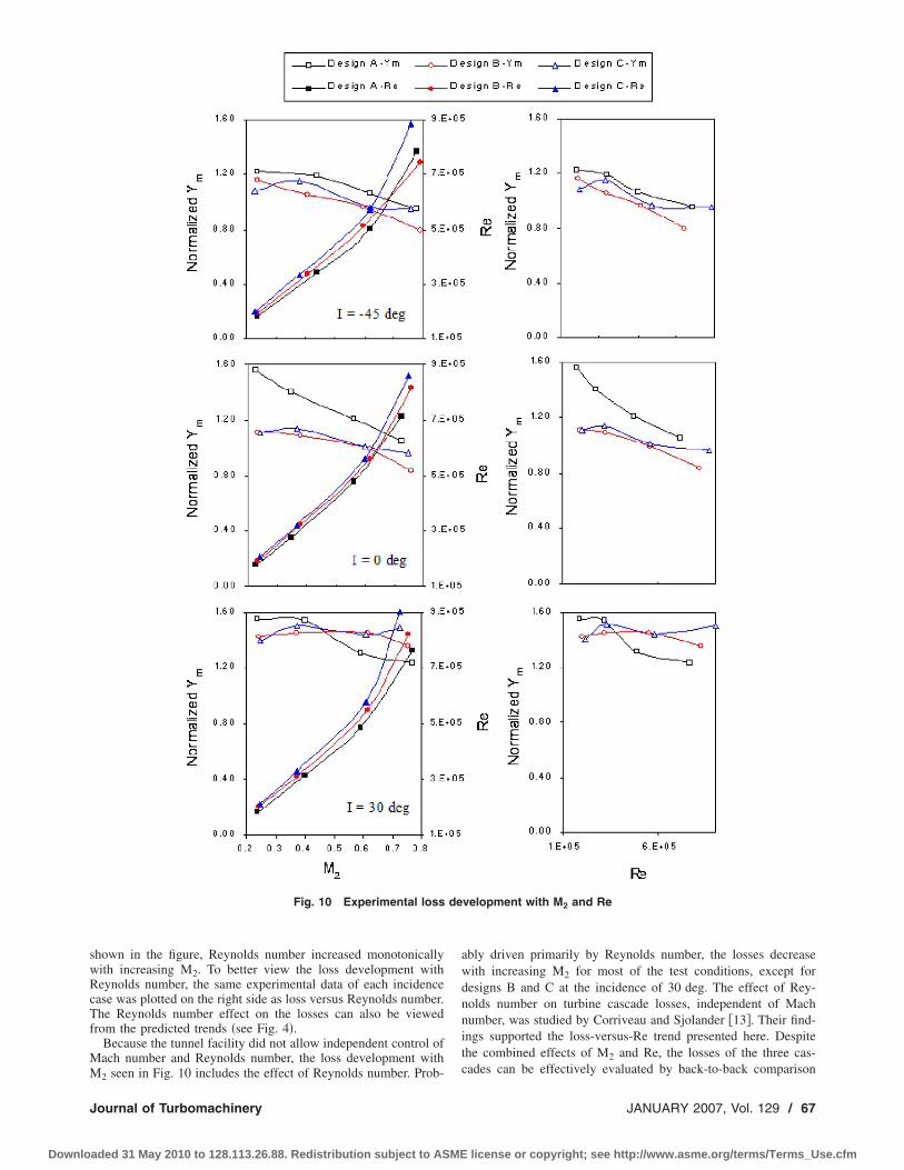
shown in the figure, Reynolds number increased monotonicallywith increasing M2. To better view the loss development withReynolds number, the same experimental data of each incidencecase was plotted on the right side as loss versus Reynolds number.The Reynolds number effect on the losses can also be viewedfrom the predicted trends �see Fig. 4�.

Because the tunnel facility did not allow independent control ofMach number and Reynolds number, the loss development withM2 seen in Fig. 10 includes the effect of Reynolds number. Prob-

ably driven primarily by Reynolds number, the losses decreasewith increasing M2 for most of the test conditions, except fordesigns B and C at the incidence of 30 deg. The effect of Rey-nolds number on turbine cascade losses, independent of Machnumber, was studied by Corriveau and Sjolander �13�. Their find-ings supported the loss-versus-Re trend presented here. Despitethe combined effects of M2 and Re, the losses of the three cas-cades can be effectively evaluated by back-to-back comparison

Fig. 10 Experimental loss development with M2 and Re



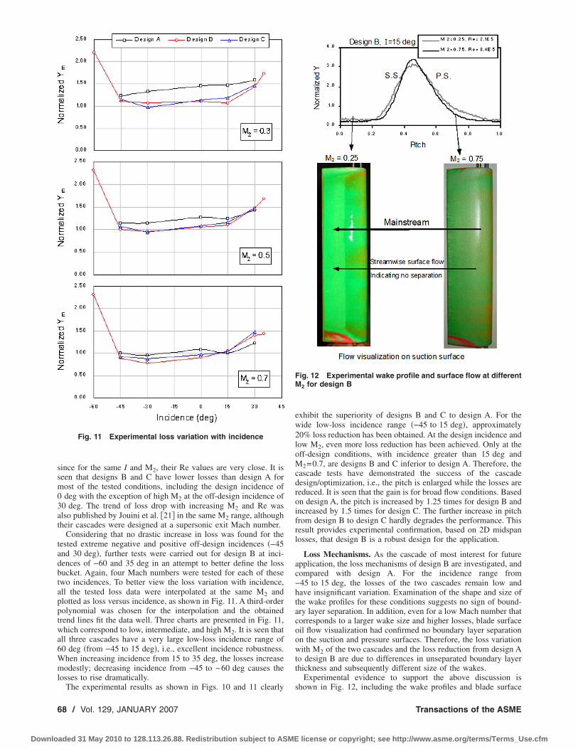
since for the same I and M2, their Re values are very close. It isseen that designs B and C have lower losses than design A formost of the tested conditions, including the design incidence of0 deg with the exception of high M2 at the off-design incidence of30 deg. The trend of loss drop with increasing M2 and Re wasalso published by Jouini et al. �21� in the same M2 range, althoughtheir cascades were designed at a supersonic exit Mach number.

Considering that no drastic increase in loss was found for thetested extreme negative and positive off-design incidences �−45and 30 deg�, further tests were carried out for design B at inci-dences of −60 and 35 deg in an attempt to better define the lossbucket. Again, four Mach numbers were tested for each of thesetwo incidences. To better view the loss variation with incidence,all the tested loss data were interpolated at the same M2 andplotted as loss versus incidence, as shown in Fig. 11. A third-orderpolynomial was chosen for the interpolation and the obtainedtrend lines fit the data well. Three charts are presented in Fig. 11,which correspond to low, intermediate, and high M2. It is seen thatall three cascades have a very large low-loss incidence range of60 deg �from −45 to 15 deg�, i.e., excellent incidence robustness.When increasing incidence from 15 to 35 deg, the losses increasemodestly; decreasing incidence from −45 to −60 deg causes thelosses to rise dramatically.

The experimental results as shown in Figs. 10 and 11 clearly

exhibit the superiority of designs B and C to design A. For thewide low-loss incidence range �−45 to 15 deg�, approximately20% loss reduction has been obtained. At the design incidence andlow M2, even more loss reduction has been achieved. Only at theoff-design conditions, with incidence greater than 15 deg andM2=0.7, are designs B and C inferior to design A. Therefore, thecascade tests have demonstrated the success of the cascadedesign/optimization, i.e., the pitch is enlarged while the losses arereduced. It is seen that the gain is for broad flow conditions. Basedon design A, the pitch is increased by 1.25 times for design B andincreased by 1.5 times for design C. The further increase in pitchfrom design B to design C hardly degrades the performance. Thisresult provides experimental confirmation, based on 2D midspanlosses, that design B is a robust design for the application.

Loss Mechanisms. As the cascade of most interest for futureapplication, the loss mechanisms of design B are investigated, andcompared with design A. For the incidence range from−45 to 15 deg, the losses of the two cascades remain low andhave insignificant variation. Examination of the shape and size ofthe wake profiles for these conditions suggests no sign of bound-ary layer separation. In addition, even for a low Mach number thatcorresponds to a larger wake size and higher losses, blade surfaceoil flow visualization had confirmed no boundary layer separationon the suction and pressure surfaces. Therefore, the loss variationwith M2 of the two cascades and the loss reduction from design Ato design B are due to differences in unseparated boundary layerthickness and subsequently different size of the wakes.

Experimental evidence to support the above discussion isshown in Fig. 12, including the wake profiles and blade surface

Fig. 11 Experimental loss variation with incidence

Fig. 12 Experimental wake profile and surface flow at differentM2 for design B



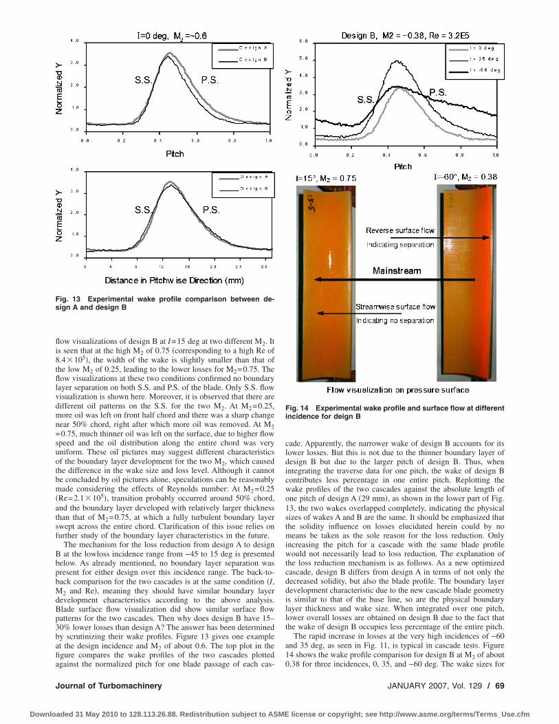
flow visualizations of design B at I=15 deg at two different M2. Itis seen that at the high M2 of 0.75 �corresponding to a high Re of8.4�105�, the width of the wake is slightly smaller than that ofthe low M2 of 0.25, leading to the lower losses for M2=0.75. Theflow visualizations at these two conditions confirmed no boundarylayer separation on both S.S. and P.S. of the blade. Only S.S. flowvisualization is shown here. Moreover, it is observed that there aredifferent oil patterns on the S.S. for the two M2. At M2=0.25,more oil was left on front half chord and there was a sharp changenear 50% chord, right after which more oil was removed. At M2=0.75, much thinner oil was left on the surface, due to higher flowspeed and the oil distribution along the entire chord was veryuniform. These oil pictures may suggest different characteristicsof the boundary layer development for the two M2, which causedthe difference in the wake size and loss level. Although it cannotbe concluded by oil pictures alone, speculations can be reasonablymade considering the effects of Reynolds number: At M2=0.25�Re=2.1�105�, transition probably occurred around 50% chord,and the boundary layer developed with relatively larger thicknessthan that of M2=0.75, at which a fully turbulent boundary layerswept across the entire chord. Clarification of this issue relies onfurther study of the boundary layer characteristics in the future.

The mechanism for the loss reduction from design A to designB at the lowloss incidence range from −45 to 15 deg is presentedbelow. As already mentioned, no boundary layer separation waspresent for either design over this incidence range. The back-to-back comparison for the two cascades is at the same condition �I,M2 and Re�, meaning they should have similar boundary layerdevelopment characteristics according to the above analysis.Blade surface flow visualization did show similar surface flowpatterns for the two cascades. Then why does design B have 15–30% lower losses than design A? The answer has been determinedby scrutinizing their wake profiles. Figure 13 gives one exampleat the design incidence and M2 of about 0.6. The top plot in thefigure compares the wake profiles of the two cascades plottedagainst the normalized pitch for one blade passage of each cas-

cade. Apparently, the narrower wake of design B accounts for itslower losses. But this is not due to the thinner boundary layer ofdesign B but due to the larger pitch of design B. Thus, whenintegrating the traverse data for one pitch, the wake of design Bcontributes less percentage in one entire pitch. Replotting thewake profiles of the two cascades against the absolute length ofone pitch of design A �29 mm�, as shown in the lower part of Fig.13, the two wakes overlapped completely, indicating the physicalsizes of wakes A and B are the same. It should be emphasized thatthe solidity influence on losses elucidated herein could by nomeans be taken as the sole reason for the loss reduction. Onlyincreasing the pitch for a cascade with the same blade profilewould not necessarily lead to loss reduction. The explanation ofthe loss reduction mechanism is as follows. As a new optimizedcascade, design B differs from design A in terms of not only thedecreased solidity, but also the blade profile. The boundary layerdevelopment characteristic due to the new cascade blade geometryis similar to that of the base line, so are the physical boundarylayer thickness and wake size. When integrated over one pitch,lower overall losses are obtained on design B due to the fact thatthe wake of design B occupies less percentage of the entire pitch.

The rapid increase in losses at the very high incidences of −60and 35 deg, as seen in Fig. 11, is typical in cascade tests. Figure14 shows the wake profile comparison for design B at M2 of about0.38 for three incidences, 0, 35, and −60 deg. The wake sizes for

Fig. 13 Experimental wake profile comparison between de-sign A and design B

Fig. 14 Experimental wake profile and surface flow at differentincidence for deign B



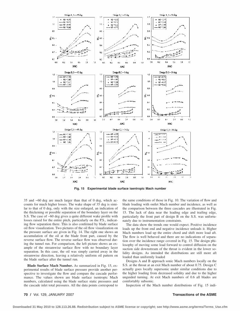
35 and −60 deg are much larger than that of 0 deg, which ac-counts for much higher losses. The wake shape of 35 deg is simi-lar to that of 0 deg, only with the size enlarged, an indication ofthe thickening or possible separation of the boundary layer on theS.S. The case of −60 deg gives a quite different wake profile withlosses raised for the entire pitch, particularly on the P.S., indicat-ing flow separation there. This is also confirmed by blade surfaceoil flow visualization. Two pictures of the oil flow visualization onthe pressure surface are given in Fig. 14. The right one shows anaccumulation of the oil at the blade front part, caused by thereverse surface flow. The reverse surface flow was observed dur-ing the tunnel run. For comparison, the left picture shows an ex-ample of the streamwise surface flow with no boundary layerseparation. In this case, the oil was simply carried away in thestreamwise direction, leaving a relatively uniform oil pattern onthe blade surface after the tunnel run.

Blade Surface Mach Number. As summarized in Fig. 15, ex-perimental results of blade surface pressure provide another per-spective to investigate the flow and compare the cascade perfor-mance. The values shown are blade surface isentropic Machnumbers, calculated using the blade surface static pressures andthe cascade inlet total pressures. All the data points correspond to

the same conditions of those in Fig. 10. The variation of flow andblade loading with outlet Mach number and incidence, as well asthe comparison between the three cascades are illustrated in Fig.15. The lack of data near the leading edge and trailing edge,particularly the front part of design B on the S.S. was unfortu-nately due to instrumentation constraints.

The data show the trends one would expect. Positive incidenceloads up the front end and negative incidence unloads it. HigherMach numbers load up the entire chord and shift more load aft.The flow is well behaved and there are no indications of separa-tion over the incidence range covered in Fig. 15. The design phi-losophy of moving some load forward to control diffusion on thesuction side downstream of the throat is evident in the lower so-lidity designs. As intended the distributions are still more aftloaded than uniformly loaded

Designs A and B approach sonic Mach numbers locally on theS.S. at the throat at an exit Mach number of about 0.75. Design Cactually goes locally supersonic under similar conditions due tothe higher loading from decreased solidity and due to the higherunguided turning. At exit Mach numbers of 0.6 all blades arecomfortably subsonic.

Inspection of the Mach number distributions of Fig. 15 indi-

Fig. 15 Experimental blade surface isentropic Mach number



cates that the quality of the flow for design B is good. Further itcan be seen that the quality of the flow at the lower solidity ofdesign C indicates that design B has some margin with respect todecreased solidity. It is therefore a robust choice to pick for futureapplications.

ConclusionExtensive cascade tests were carried out to determine the per-

formance of three steam turbine nozzle cascades. The three cas-cades are designed for the same inlet and exit vector diagrams.They have the same axial chord, but the solidity is varied from1.22 to 0.93. For all three cascades, experimental results haveshown a wide lowloss incidence range from −45 to 15 deg at thetested outlet Mach numbers ranging from 0.2 to 0.8. At thesebroad conditions, the boundary layer is well controlled withoutseparation such that the losses are low. Most importantly, a 15–30% profile loss reduction has been obtained while reducing thesolidity on the new cascades. The larger improvements are at thelower Mach numbers. As the best candidate cascade for applica-tion, design B was tested at two more off-design incidences �−60and 35 deg� to more fully document the loss bucket.

Wake profile comparison and blade surface flow visualizationare successfully used in conjunction to help understand the flowand the loss reduction mechanism. It is confirmed that design Bhas the same boundary layer characteristics as the baseline. Thewakes of designs A and B are the same size but since design B hasa larger pitch and fewer blades and wakes for a given applicationthe overall losses are lower.

Cascade design optimization led to more tangential stagger andhigher unguided turning for the lower solidity cascades. The load-ing on the lower solidity cascades was brought forward somewhatto control the suction surface diffusion downstream of the throatto avoid separation and high losses. This strategy has proved ef-fective in developing low loss cascades at low solidities. The lowsolidities allow a reduction in parts count for reduced cost at ahigh level of efficiency.

It is also of interest to point out that a design which is based onthe use of a 2D Euler flow solver with boundary layer and losscalculations proved to be sufficient to give optimized bladeshapes, as verified by the experiment.

AcknowledgmentThis work was sponsored by GE Energy. Stephen Guillot and

Troy Jones of Techsburg, Inc. provided significant support for theexperimental work. Their help is gratefully acknowledged.

NomenclatureAC � axial chordAR � aspect ratio

C � true chordCp � pressure coefficient= Ps / Pt1H � blade spanI � incidence angle

M � Mach numberP.S. � pressure surface

Ps � static pressurePt � total pressure

Re � Reynolds number �based on true chord andoutlet condition�

t � pitchS.S. � suction surface

s � throatTu � free-stream turbulence intensityX � distance in axial directionY � loss coefficient= �Pt1

− Pt2� / �Pt1

− Ps2�

Ym � mix-out losscoefficient= �Pt1

− Pt2m� / �Pt1

− Ps2m�

� � stagger angle� � solidity, �=C / t

Subscripts1 � cascade inlet2 � cascade inletm � mix-outis � isentropic

References�1� Cobley, K., Coleman, N., Siden, G., and Arndt, N., 1997, “Design of New

Three Stage Low Pressure Turbine for the BMW Rolls-Royce BR715 Turbo-fan Engine,” ASME Paper No. 97-GT-419.

�2� Curtis, E. M., Hodson, H. P., Banieghbal, M. R., Denton, J. D., and Howell, R.J., 1996, “Development of Blade Profiles for Low Pressure Turbine Applica-tion,” ASME Paper No. 96-GT-358.

�3� Tsujita, H., Mizuki, S., and Yamamoto, A., 2004, “Numerical Investigation ofBlade Profile Effects on Aerodynamic Performance of Ultra-Highly LoadedTurbine Cascades,” ASME Paper No. GT2004–53429.

�4� Moustapha, S. H., Paron, G. J., and Wade, J. H.T., 1985, “Secondary Flow inCascade of Highly Loaded Turbine Blades,” ASME Paper No. 85-GT-135.

�5� Solomon, W. J., 2000, “Effects of Turbulence and Solidity on the BoundaryLayer Development in a Low Pressure Turbine,” ASME Paper No. 2000-GT-273.

�6� Solomon, W. J., 2002, “Performance Characteristics of a Reduced SolidityLow Pressure Turbine,” ICAS 2002 Congress, pp. 5112.1–5112.10.

�7� Howell, R. J., Ramesh, O. N., Hodson, H. P., Harvey, N. W., and Schulte, V.,2000, “High Lift and Aft Loaded Profiles for Low Pressure Turbines,” ASMEPaper No. 2000-GT-261.

�8� Haselbach, F., Schiffer, H., Horsman, M., Dressen, S., Harvey, N., and Read,S., 2002, “The Application of Ultra High Lift Blading in the BR715 LP Tur-bine,” ASME J. Turbomach., 124, pp. 45–51.

�9� Howell, R. J., Hodson, H. P., Schulte, V., Stieger, R. D., Schiffer, H., Hasel-bach, F., and Harvey, N. W., 2002, “Boundary Layer Development in theBR710 and BR715 LP Turbines—The Implementation of High-Lift and Ultra-High-Lift Concepts,” ASME J. Turbomach., 124, pp. 385–392.

�10� Hodson, H. P., and Howell, R. J., 2001, “High Lift Low Pressure Turbines,”NASA/CP-2001-210888.

�11� Gonzalez, P., Ulizar, I., Vazquez, R., and Hodson, H. P., 2002, “Pressure andSuction Surfaces Redesign for High-Lift Low-Pressure Turbines,” ASME J.Turbomach., 124, pp. 161–166.

�12� Houtermans, R., Coton, T., and Arts, T., 2003, “Aerodynamic Performance ofa Very High Lift LP Turbine Blade With Emphasis on Separation Prediction,”ASME Paper No. GT2003-38802.

�13� Corriveau, D., and Sjolander, S. A., 2003, “Influence of Loading Distributionon The Performance of Transonic HP Turbine Blades,” ASME Paper No.GT2003-38079.

�14� Patterson, D. J., and Hoeger, M., 1986, “The Effect of Reynolds Number andVelocity Distribution on LP Turbine Cascade Performance,” ASME Paper No.86-GT-271.

�15� Hashimoto, K., and Kimura, T., 1984, “Preliminary Study on Forward LoadedCascades Designed With Inverse Method for Low Pressure Turbine,” ASMEPaper No. 84-GT-65.

�16� Hoheisel, H., Kiock, R., Lichtfuss, H. J., and Fottner, L., 1987, “Influence ofFree-Stream Turbulence and Blade Pressure Gradient on Boundary Layer andLoss Behavior of Turbine Cascades,” ASME J. Turbomach., 109, pp. 210–219.

�17� Boss, M., Hofer, D., Gazzillo, C., and Jacobs, J., 2002, “Advances inCombined-Cycle Steam Turbines,” Power-Gen International 2002, Orlando,FL.

�18� Boss, M., 2003, “Steam Turbine Technology Heats Up,” PEi Mag., April.�19� Drela, M., and Youngren, H., 1996, A User’s Guide to MISES 2.4, MIT Com-

putational Aerospace Sciences Laboratory, Cambridge, MA.�20� Sieverding, C. H., 1993, “Subsonic-Choked �Turbine� Cascades,” Advanced

Methods for Cascade Testing, AGARD-AG-328, p. 23.�21� Jouini, D. B. M., Sjolander, S. A., and Moustapha, S. H., 2001, “Midspan

Flow-Field Measurements for Two Transonic Linear Turbine Cascades at Off-Design Conditions,” ASME Paper No. 2001-GT-0493.



Roque Corral1


Juan Manuel Gallardo

Carlos Vasco

Technology and Methods Department,Industria de Turbopropulsores S.A.,

28830 Madrid, Spain

Aeroelastic Stability ofWelded-in-Pair Low PressureTurbine Rotor Blades:A Comparative Study UsingLinear MethodsThe aerodynamic damping of a modern low pressure turbine bladed-disk with interlockrotor blades is compared for the first time to that obtained when the rotor blades arewelded in pairs through the lateral face of the shroud. The damping is computed solvingthe linearized Reynolds averaged Navier-Stokes equations on a moving grid. First thebasics of the stabilizing mechanism of welding the rotor blades in pairs is investigatedusing two-dimensional analyses and the Panovsky and Kielb method. It is concluded thatthe stabilizing effect is due to the suppression of unsteady perturbations in one out of thetwo passages providing for the first time a physical explanation to engine data. Three-dimensional effects are then studied using the actual mode shapes of two bladed disksdiffering solely in the shroud boundary conditions. It is concluded that the increase in theaerodynamic damping, due to the modification of the mode shapes caused by welding therotor blades in pairs, is smaller than that due to the overall raise of the reduced frequen-cies of a bladed disk with an interlock design. The modification of the flutter boundariesdue to mistuning effects is assessed using the reduced order model known as the Funda-mental Mistuning Model. A novel extension of the critical reduced frequency stabilitymaps accounting for mistuning effects is derived and applied for both, the freestandingand welded-in-pair airfoils. The stabilizing effect of mistuning is clearly seen in thesemaps. Finally, the effect of mistuning on low-pressure-turbine bladed disks is studied. Itis shown that the modification on the stability limit of the interlock bladed disk is negli-gible, while for the welded-in-pair configuration a 0.15% increase of the damping rela-tive to the critical damping is found. This qualitative difference between both configura-tions had not been reported before. �DOI: 10.1115/1.2366512�

IntroductionFlutter has been a problem traditionally associated with com-

pressor and fan blades. However, the steady trend during the lastdecades to design high-lift, highly loaded low pressure turbines�LPTs�, with the final aim of reducing their cost and weight, whilekeeping the same efficiency, has led to a reduction of the bladeand disk thicknesses and an increase of the blade aspect ratio.Both factors tend to lower the stiffness of the bladed-disk assem-bly and therefore its natural frequencies. The decrease of themaximum relative thickness of LPT midsections during the lasttwo decades is depicted in Fig. 1.

As a result of the aforementioned evolution, vanes and rotorblades of the latter stages of modern LPTs of large commercialturbofan engines, which may be designed with aspect ratios of upto six, may potentially flutter and undergo alternate stresses simi-lar to those encountered in fans and compressors.

Vibration control of shrouded LPT blades may be accomplishedusing either cantilever, interlock or welded-in-pairs rotor blades�see Fig. 2�. Flat sided shrouds may vibrate freely even for verysmall clearances especially for low inter blade phase angles�IBPA� and provide little control over the vibration characteristics

of the bladed disk. To remedy this deficiency z-shaped shrouds�interlocks� were designed with the aim of remaining tight duringthe whole flight envelope. This type of design significantly modi-fies the vibration characteristics of cantilever blades, however, themode shapes of a given family may significantly vary with thenodal diameter and induce bending-torsion coupling. Finally, pairsof rotor blades welded in the tip shroud were devised as a practi-cal alternative to control the vibration characteristics of LPTbladed disks and may be seen in some modern turbofan engines.This latter configuration substantially modifies as well the modeshapes and frequencies of the base line �cantilever� and interlocksolutions.

It is well known that flutter boundaries are very sensitive toblade mode shapes and that the reduced frequency plays a second-ary role. A comprehensive numerical study of the influence ofboth parameters for LPT airfoils was performed by Panovsky andKielb �1� and supported by experimental work �2�.

The beneficial effect of grouping the airfoils in packets was firstdemonstrated by Whitehead and Evans �3�. Kahl �4� studied thestability of a LPT sectored vane of three airfoils and later onChernysheva et al. �5� extended the stability studies to packets ofsix vanes using the Panovsky and Kielb �PK� method.

However, in an actual machine rotor blades are never exactlyidentical because of manufacturing imperfections, which result inslightly different natural frequencies and phase shifts of theblades. There is numerical �6–8� and experimental �2� evidencethat mistuning has a strong beneficial effect on self-excited vibra-

1Also Associate Professor at the Department of Engine Propulsion and FluidDynamics of the School of Aeronautics, UPM.

Contributed by the International Gas Turbine Institute �IGTI� of ASME for pub-lication in the JOURNAL OF TURBOMACHINERY. Manuscript received October 1, 2003;final manuscript received March 1, 2004. IGTI Review Chair: A. J. Strazisar. Paperpresented at the International Gas Turbine and Aeroengine Congress and Exhibition,Vienna, Austria, June 13–17, 2004, Paper No. 2004-GT-54119.



tions. However, the attempts to analyze �9� or devise design meth-ods �10� retaining the effect of mistuning are scarce.

Flutter analyses are usually performed in the frequency domainmaking use of the hypothesis of linearity to dramatically reducethe computational cost of non-linear single-passage or whole an-nulus computations. Mistuned aerodynamic models make use ofthe hypothesis of linearity as well as precomputing the aerody-namic damping in traveling-wave form for a prescribed frequency,and deriving the damping of the mistuned case expanding theeigenmodes of the mistuned problem in traveling waves �11,10�which is several orders of magnitude less expensive than comput-ing the whole mistuned wheel �9�.

The use of welded-in-pair rotor blades in large civil turbofansdates back to the early 1990s. However, the rationale of its stabi-lizing effect has been poorly understood and has never been re-ported before. The aim of this work is to investigate, using nu-merical tools, the influence of pairing the rotor blades on theaerodynamic damping of a typical LPT bladed disk and comparethe results with the equivalent, and more widespread, interlockconfiguration.

In this work, the analysis methodology is presented first. Then atypical airfoil is used to analyze the stabilizing effect of weldingthe airfoils in pairs from a two-dimensional point of view usingsimplified methods. A significant part of the article is focused onthe analysis of realistic bladed disks with special emphasis in thecomparison of the relative merits of interlock and welded-in-pairrotor blades. In this study we retained three-dimensional featuresboth in the structural dynamics and aerodynamics, where viscouseffects are also accounted for. Finally, the beneficial effect of mis-

tuning on the stability is assessed, both for a standard two-dimensional airfoil and for realistic bladed disks. The use of thePK method in this part, retaining the effect of mistuning, is novel.The paper is closed deriving some final conclusions.

Numerical Formulation

Linearized Navier-Stokes Equations. The three-dimensionalNavier-Stokes equations in conservative form for an arbitrary con-trol volume may be written as:

d

dt��

Ud� +��

�f − Uvx,g − Uvy,h − Uvz� . dA = 0 �1�

where U is the vector of conservative variables, f, g, and h thesum of the inviscid and viscous fluxes, � the flow domain, � itsboundary, dA the differential area pointing outward to the bound-ary and vx, vy and vz the three components of the boundary ve-locity. Now we may decompose the flow into two parts: a steadyor mean background flow, plus a small but periodic unsteady per-turbation, which in turn may be expressed as a Fourier series intime. If we retain just the first harmonic any variable may beexpressed as:

U�x,t� = U0�x� + Re�u�x�ei�t� �2�

where U0 represents the background flow and u is the complexperturbation. The Navier-Stokes equations may then be linearizedabout the mean flow to obtain:

� d

d�+ i��

�

ud� +��

� �f

�Uu,

�g

�Uu,

�h

�Uu� . dA + i��

�

U0d��

+��

�f0,g0,h0� . dA� = i��

U0x� . dA �3�

which is a linear equation of complex coefficients and where thefirst term is an additional time derivative added to solve the equa-tions marching in the pseudo-time �.

Spatial Discretization. The code used here �Mu2s2T−L� solvesthe three-dimensional linearized Navier-Stokes equations in con-servative form �12�. The spatial discretization is obtained linear-izing the discretized equations of the non-linear version of thecode Mu2s2T �13�, from which the background solution is ob-tained. The spatial domain is discretized using hybrid unstructuredgrids that may contain cells with an arbitrary number of faces andthe solution vector is stored at the vertexes of the cells. The codeuses an edge-based data structure, a typical grid is discretized byconnecting the median dual of the cells surrounding an internalnode �Fig. 3�. For the node i the semi-discrete form of Eq. �3� canbe written as

Fig. 1 Evolution of LPT mid-section airfoils during the last twodecades

Fig. 2 Sketch of cantilever, welded-in-pair and interlockshrouds

Fig. 3 Typical hybrid-cell grid and associated dual mesh



d��iui�d�

+ �j=1

nedges 1

2Sij�Fi + F j� − Dij = S�ui� �4�

where Sij is the area associated with the edge ij, and nedges thenumber of edges that surround node j. The resulting numericalscheme is cell centered in the dual mesh and second-order accu-rate. It may be shown that for triangular grids the scheme isequivalent to a cell vertex finite volume scheme. A blend of sec-

ond and fourth order artificial dissipation terms, Dij, is added tocapture shock waves and prevent the appearance of high fre-quency modes in smooth flow regions, respectively. The second-order terms are activated in the vicinity of shock waves by meansof a pressure-based sensor and locally the scheme reverts to firstorder in these regions. The artificial dissipation terms can be writ-ten as

Dij = AijSij��ij�2��u j − ui� − �ij

�4��Lj − Li�� 5�

where �ij�2� and �ij

�4� are the average of the artificial viscosity co-efficients in the nodes i and j. Aij is a 5�5 matrix that plays therole of a scaling factor. If Aij= �u+c�ijI, where I is the identitymatrix, the standard scalar formulation of the numerical dissipa-tion terms �14� is recovered. When Aij is chosen as the Roematrix �15� the matricial form of the artificial viscosity �16� isobtained. The scalar version of the numerical diffusion terms hasbeen used in this work since the difference between both ap-proaches is negligible for the Mach numbers of interest �17� and ismore robust.

The viscous fluxes can be evaluated in a number of ways. Thegradients of the flow variables are approximated at the nodes us-ing the divergence theorem in the same way that the convectivefluxes are computed. Then an approximation of the gradients atthe midpoint of the edge is obtained by a simple average,

�Uij =1

2��Ui + �Uj� �6�

The Baldwin-Lomax turbulence model �18� has been used for thesteady flow computations and the turbulence viscosity has beenfrozen in the linear version of the code.

Temporal Discretization. Equation �4� can be expressed incompact form as

d��iui�d�

= R�u� = C�u� + H�u� + S�u� �7�

where the residual can be split in the convective, C, the numericaldiffusion and viscous, H, parts and a source term S. The integra-tion in time is performed using an explicit five stage Runge-Kuttascheme, where the artificial viscosity terms are evaluated only inthree stages of the Runge-Kutta.

The scheme is second-order accurate in time. Implicit residualsmoothing and full coarsening multigrid may be used to increasethe stability limit of the scheme and speed up its convergence. Amore detailed description of the numerical scheme and details ofthe validation process may be found in �12�.

Boundary Conditions. The exact, 2D, unsteady, non-reflectingboundary conditions �19� have been used at the inlet and outlet ina plane by plane basis. At the solid walls half volumes associatedwith the wall nodes are used to march in pseudo time. For inviscidsimulations the unsteady fluxes are imposed at the boundarieswhile for viscous cases the velocity is imposed at the boundarynodes. The code uses phase-shifted boundary conditions in theperiodic boundaries to simulate annular cascades of airfoils vibrat-ing sinusoidally with a common angular frequency, �, and com-mon IBPA.

Two-Dimensional Analysis Methodology

Description of the Method. Using flutter stability maps,Panovsky and Kielb �1� showed that the mode shape and the re-duced frequency are the basic parameters that control the stabilityof a two-dimensional LPT section. Since one of the aims of thiswork was to understand the stability of welded-in-pair rotorblades, including the influence of the torsion center and reducedfrequency, it was decided to adopt this simplified approach.

Following the PK approach only the unsteady pressure fieldsassociated with two orthogonal bending directions and the torsionabout a given point, P, for a reference displacement need to becomputed for each IBPA �see Fig. 4�. The unsteady pressure as-sociated with the motion of the airfoil as a rigid body about anarbitrary torsion axis, O, is computed as a linear combination ofthe three reference solutions.

The main differences of the present method with the originalapproach are the systematic use of viscous simulations and theextension of the analyses to pairs of airfoils moving as a rigidbody. However, instead of using an influence coefficient techniqueto simulate the sector as in �5�, we have included pairs of airfoilsvibrating as a rigid body to emulate the dynamic behavior of rotorblades welded in pairs.

Underlying Hypothesis. Although the details of the methodare well known and may be found in �1�, the main hypotheses ofthe approach are revisited here to check its validity for the presentstudy:

1. The superposition principle holds. This is not usually a prob-lem for LPTs with subsonic flows and small vibration am-plitudes.

2. The airfoil moves as a rigid body. For elongated, high aspectratio LPT airfoils, with a similar stiffness along the chordand without constraints at the tip, it is unusual to have localmodes. Figure 5 shows the first bending �left� and first tor-sion �right� mode shapes of a welded-pair bladed disk on the

Fig. 4 Definition of fundamental mode shapes



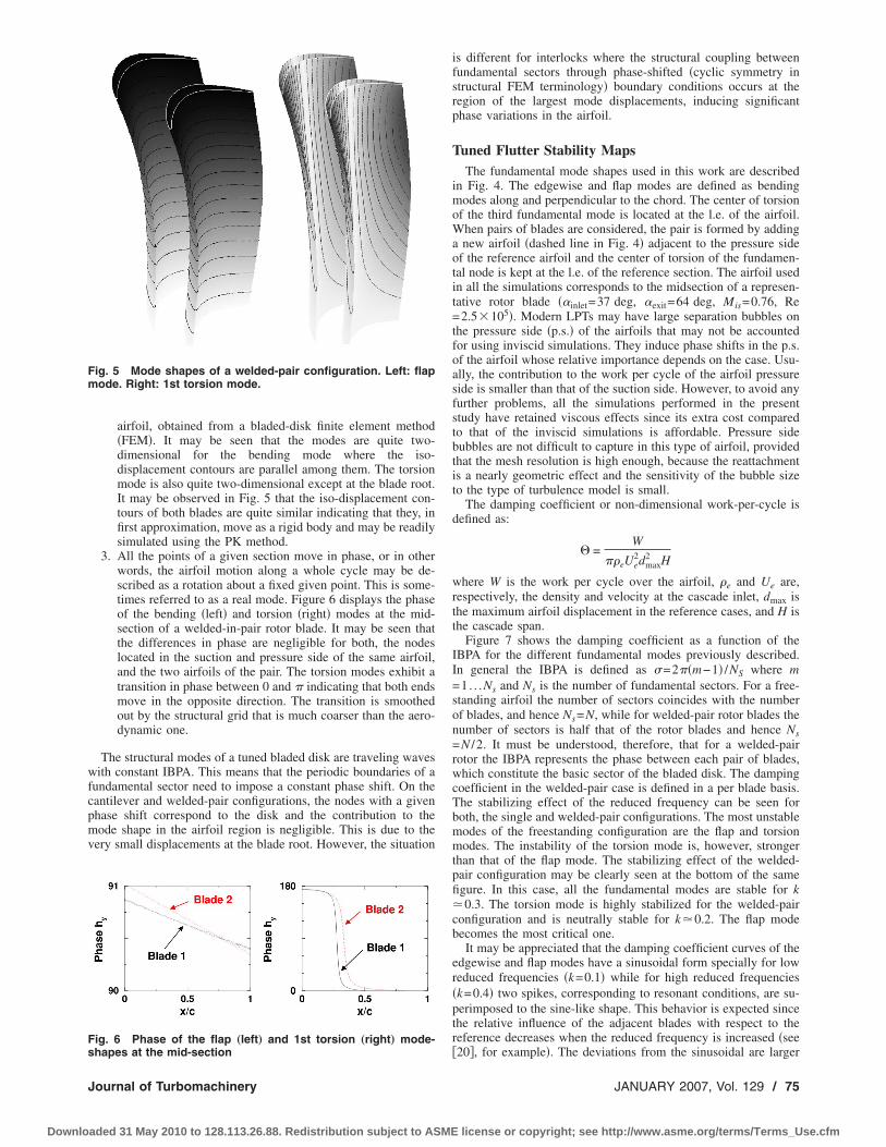
airfoil, obtained from a bladed-disk finite element method�FEM�. It may be seen that the modes are quite two-dimensional for the bending mode where the iso-displacement contours are parallel among them. The torsionmode is also quite two-dimensional except at the blade root.It may be observed in Fig. 5 that the iso-displacement con-tours of both blades are quite similar indicating that they, infirst approximation, move as a rigid body and may be readilysimulated using the PK method.

3. All the points of a given section move in phase, or in otherwords, the airfoil motion along a whole cycle may be de-scribed as a rotation about a fixed given point. This is some-times referred to as a real mode. Figure 6 displays the phaseof the bending �left� and torsion �right� modes at the mid-section of a welded-in-pair rotor blade. It may be seen thatthe differences in phase are negligible for both, the nodeslocated in the suction and pressure side of the same airfoil,and the two airfoils of the pair. The torsion modes exhibit atransition in phase between 0 and � indicating that both endsmove in the opposite direction. The transition is smoothedout by the structural grid that is much coarser than the aero-dynamic one.

The structural modes of a tuned bladed disk are traveling waveswith constant IBPA. This means that the periodic boundaries of afundamental sector need to impose a constant phase shift. On thecantilever and welded-pair configurations, the nodes with a givenphase shift correspond to the disk and the contribution to themode shape in the airfoil region is negligible. This is due to thevery small displacements at the blade root. However, the situation

is different for interlocks where the structural coupling betweenfundamental sectors through phase-shifted �cyclic symmetry instructural FEM terminology� boundary conditions occurs at theregion of the largest mode displacements, inducing significantphase variations in the airfoil.

Tuned Flutter Stability MapsThe fundamental mode shapes used in this work are described

in Fig. 4. The edgewise and flap modes are defined as bendingmodes along and perpendicular to the chord. The center of torsionof the third fundamental mode is located at the l.e. of the airfoil.When pairs of blades are considered, the pair is formed by addinga new airfoil �dashed line in Fig. 4� adjacent to the pressure sideof the reference airfoil and the center of torsion of the fundamen-tal node is kept at the l.e. of the reference section. The airfoil usedin all the simulations corresponds to the midsection of a represen-tative rotor blade ��inlet=37 deg, �exit=64 deg, Mis=0.76, Re=2.5�105�. Modern LPTs may have large separation bubbles onthe pressure side �p.s.� of the airfoils that may not be accountedfor using inviscid simulations. They induce phase shifts in the p.s.of the airfoil whose relative importance depends on the case. Usu-ally, the contribution to the work per cycle of the airfoil pressureside is smaller than that of the suction side. However, to avoid anyfurther problems, all the simulations performed in the presentstudy have retained viscous effects since its extra cost comparedto that of the inviscid simulations is affordable. Pressure sidebubbles are not difficult to capture in this type of airfoil, providedthat the mesh resolution is high enough, because the reattachmentis a nearly geometric effect and the sensitivity of the bubble sizeto the type of turbulence model is small.

The damping coefficient or non-dimensional work-per-cycle isdefined as:

=W

�eUe2dmax

2 H

where W is the work per cycle over the airfoil, e and Ue are,respectively, the density and velocity at the cascade inlet, dmax isthe maximum airfoil displacement in the reference cases, and H isthe cascade span.

Figure 7 shows the damping coefficient as a function of theIBPA for the different fundamental modes previously described.In general the IBPA is defined as �=2��m−1� /NS where m=1. . .Ns and Ns is the number of fundamental sectors. For a free-standing airfoil the number of sectors coincides with the numberof blades, and hence Ns=N, while for welded-pair rotor blades thenumber of sectors is half that of the rotor blades and hence Ns=N /2. It must be understood, therefore, that for a welded-pairrotor the IBPA represents the phase between each pair of blades,which constitute the basic sector of the bladed disk. The dampingcoefficient in the welded-pair case is defined in a per blade basis.The stabilizing effect of the reduced frequency can be seen forboth, the single and welded-pair configurations. The most unstablemodes of the freestanding configuration are the flap and torsionmodes. The instability of the torsion mode is, however, strongerthan that of the flap mode. The stabilizing effect of the welded-pair configuration may be clearly seen at the bottom of the samefigure. In this case, all the fundamental modes are stable for k0.3. The torsion mode is highly stabilized for the welded-pairconfiguration and is neutrally stable for k0.2. The flap modebecomes the most critical one.

It may be appreciated that the damping coefficient curves of theedgewise and flap modes have a sinusoidal form specially for lowreduced frequencies �k=0.1� while for high reduced frequencies�k=0.4� two spikes, corresponding to resonant conditions, are su-perimposed to the sine-like shape. This behavior is expected sincethe relative influence of the adjacent blades with respect to thereference decreases when the reduced frequency is increased �see�20�, for example�. The deviations from the sinusoidal are larger

Fig. 5 Mode shapes of a welded-pair configuration. Left: flapmode. Right: 1st torsion mode.

Fig. 6 Phase of the flap „left… and 1st torsion „right… mode-shapes at the mid-section



for the torsion mode. For the welded-pair configuration, the situ-ation is somewhat more complex and the damping curves exhibitseveral peaks. Due to the spiky shape of the damping curves, wehave consistently computed them using 16 IBPAs.

Figure 8 �left� shows the critical reduced frequency stabilitymap for a freestanding airfoil. The reduced frequency assigned toevery point of the plot is the minimum that ensures that the vibra-tion of the airfoil as a rigid body about this center of torsion isstable. The tie-dye plots are used computing the actual reducedfrequency and torsion center for the section of interest and com-paring the actual reduced frequency with that of the plot. Themiddle section represents the reference section. It can be seen thatthe airfoil is highly unstable in torsion, and increasing the reducedfrequency enlarges the stable region. It is also worth noting that

while the axial mode �bending in the x direction� is quite stable,the flex mode �bending in the y direction� nearly coincides withthe most unstable direction. This may be inferred by realizing thata torsion axis at infinity �y→�, for instance� generates a purebending mode.

Figure 8 �right� shows the equivalent map for a pair of airfoilsmoving as a rigid body. The lower airfoil of the pair correspondsto the lower section of the figure. The increase in the aerodynamicdamping in all the modes with respect the single blade configura-tion is clearly seen. For k=0.4, the airfoil is stable for torsionmodes whose center of torsion lies in the vicinity of the welded-pair passage and in a wide range of bending directions. The mostunstable direction �bending� coincides with that of the flex mode.

Fig. 7 Damping as a function of IBPA for the three fundamental modes. Top: freestanding airfoil. Bottom: welded-in-pairconfiguration.

Fig. 8 Critical reduced frequency maps for the freestanding „left… and welded-in-pair „right… configurations



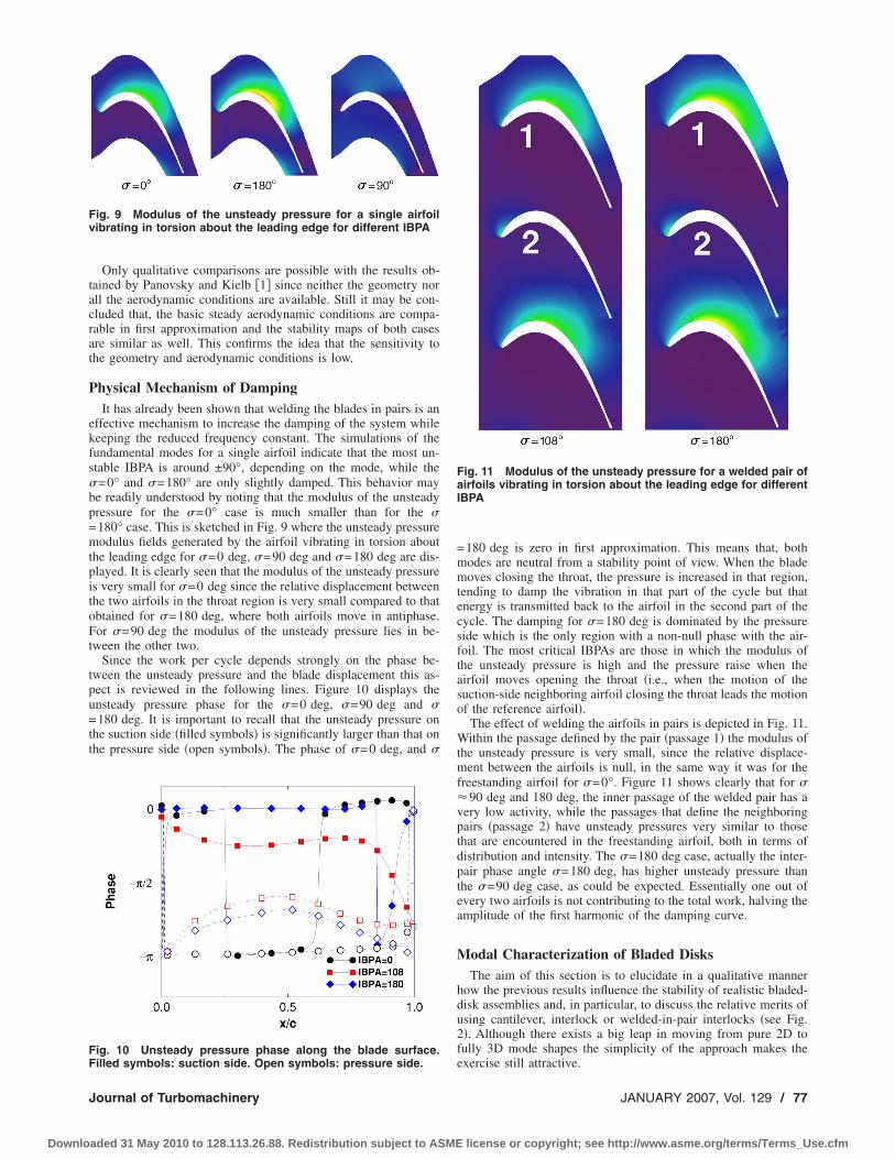
Only qualitative comparisons are possible with the results ob-tained by Panovsky and Kielb �1� since neither the geometry norall the aerodynamic conditions are available. Still it may be con-cluded that, the basic steady aerodynamic conditions are compa-rable in first approximation and the stability maps of both casesare similar as well. This confirms the idea that the sensitivity tothe geometry and aerodynamic conditions is low.

Physical Mechanism of DampingIt has already been shown that welding the blades in pairs is an

effective mechanism to increase the damping of the system whilekeeping the reduced frequency constant. The simulations of thefundamental modes for a single airfoil indicate that the most un-stable IBPA is around ±90°, depending on the mode, while the�=0° and �=180° are only slightly damped. This behavior maybe readily understood by noting that the modulus of the unsteadypressure for the �=0° case is much smaller than for the �=180° case. This is sketched in Fig. 9 where the unsteady pressuremodulus fields generated by the airfoil vibrating in torsion aboutthe leading edge for �=0 deg, �=90 deg and �=180 deg are dis-played. It is clearly seen that the modulus of the unsteady pressureis very small for �=0 deg since the relative displacement betweenthe two airfoils in the throat region is very small compared to thatobtained for �=180 deg, where both airfoils move in antiphase.For �=90 deg the modulus of the unsteady pressure lies in be-tween the other two.

Since the work per cycle depends strongly on the phase be-tween the unsteady pressure and the blade displacement this as-pect is reviewed in the following lines. Figure 10 displays theunsteady pressure phase for the �=0 deg, �=90 deg and �=180 deg. It is important to recall that the unsteady pressure onthe suction side �filled symbols� is significantly larger than that onthe pressure side �open symbols�. The phase of �=0 deg, and �

=180 deg is zero in first approximation. This means that, bothmodes are neutral from a stability point of view. When the blademoves closing the throat, the pressure is increased in that region,tending to damp the vibration in that part of the cycle but thatenergy is transmitted back to the airfoil in the second part of thecycle. The damping for �=180 deg is dominated by the pressureside which is the only region with a non-null phase with the air-foil. The most critical IBPAs are those in which the modulus ofthe unsteady pressure is high and the pressure raise when theairfoil moves opening the throat �i.e., when the motion of thesuction-side neighboring airfoil closing the throat leads the motionof the reference airfoil�.

The effect of welding the airfoils in pairs is depicted in Fig. 11.Within the passage defined by the pair �passage 1� the modulus ofthe unsteady pressure is very small, since the relative displace-ment between the airfoils is null, in the same way it was for thefreestanding airfoil for �=0°. Figure 11 shows clearly that for ��90 deg and 180 deg, the inner passage of the welded pair has avery low activity, while the passages that define the neighboringpairs �passage 2� have unsteady pressures very similar to thosethat are encountered in the freestanding airfoil, both in terms ofdistribution and intensity. The �=180 deg case, actually the inter-pair phase angle �=180 deg, has higher unsteady pressure thanthe �=90 deg case, as could be expected. Essentially one out ofevery two airfoils is not contributing to the total work, halving theamplitude of the first harmonic of the damping curve.

Modal Characterization of Bladed DisksThe aim of this section is to elucidate in a qualitative manner

how the previous results influence the stability of realistic bladed-disk assemblies and, in particular, to discuss the relative merits ofusing cantilever, interlock or welded-in-pair interlocks �see Fig.2�. Although there exists a big leap in moving from pure 2D tofully 3D mode shapes the simplicity of the approach makes theexercise still attractive.

Fig. 9 Modulus of the unsteady pressure for a single airfoilvibrating in torsion about the leading edge for different IBPA

Fig. 10 Unsteady pressure phase along the blade surface.Filled symbols: suction side. Open symbols: pressure side.

Fig. 11 Modulus of the unsteady pressure for a welded pair ofairfoils vibrating in torsion about the leading edge for differentIBPA



The bladed-disk assembly considered in this study is represen-tative of the first stages of modern LPTs. The vibration character-istics of the cantilever, interlock and welded-pair configurationshave been obtained with the same grid. The boundary condition inthe contact nodes between the blade and the disk enforces that thedisplacements of these are identical in both solids. In the contactfaces of the interlock, cyclic symmetry, following the structuralFEM terminology, or phase-shifted boundary conditions, in theaerodynamic terminology, are used. This simplifying hypothesis ismade to avoid the generation of non-linear models where the con-cepts of natural frequency and mode shape need to be re-interpreted. However, special care has been taken in this case tomatch the experimental frequencies of the rotor.

Figure 12 displays the non-dimensional frequency of the firstmode families for the cantilever �left�, welded-pair �middle�, andinterlock �right� configurations as a function of the non-dimensional nodal diameter, ND /NDmax, where NDmax=N /2 forthe cantilever and interlock configurations and NDmax=N /4 forwelded pairs. Several conclusions may be drawn upon inspectionof this figure and the mode shapes, not shown here for the sake ofbrevity,

1. The disk is very stiff compared to the blades. This may beseen in the mode shapes, that show very small displacementsof the disk, as well as in the frequency nodal diameter dia-gram that displays a high number of modes with nearly thesame frequency within the same family.

2. The flap and edgewise modes of the welded-pair configura-tion have slightly higher frequencies than the cantilever onein the high ND region, which is the relevant one from aflutter point of view.

3. The frequency of the first torsion �1T� mode of the welded-pair configuration is lower than that of the cantilever con-figuration in the whole range of ND.

4. The disk dominated modes of the welded-pair configurationare shifted to the right in Fig. 12 due to the rescaling withNDmax of the horizontal axis.

5. The interlock provides an effective means to raise the fre-quencies of the assembly. The highest nodal diameters of thefirst family corresponding to shroud dominated modes.

Application of the PK MethodThe objective of this section is to apply the results obtained

with the PK method to realistic bladed disks. To simplify thediscussion it will be assumed that the bending direction of theflap-wise and edge-wise modes approximately coincides with thatof the fundamental modes, i.e., the direction defined by the linethat joins the l.e. and t.e. of the airfoil and its normal �dashed linesin Fig. 8�. The rationale of this assumption is based on the factthat these directions approximately match those of the principaldirections of the airfoil, which are the airfoil natural directions ofvibration.

It is clearly seen from Fig. 8, left, that the freestanding configu-ration is unstable. The reduced frequency of the first flap mode isless than 0.2 �see Fig. 12, left� while the minimum reduced fre-quency to stabilize a flap mode is approximately 0.5. The firsttorsion mode is probably unstable as well. While the actual valueof the reduced frequency for high ND is about 0.6, the torsioncenter lies in a region of the tie-dye plot of high gradients wherethe critical reduced frequency may raise up to 1.2. The welded-pair configuration is better from a stability point of view than thefreestanding one.

Figure 8 �right� depicts the critical reduced frequency map forthe welded-in-pair configuration. We have superimposed on it thelocation of the torsion centers of the most unstable modes of thefirst three family modes obtained from a 3D FEM �see Fig. 13,right� to compare the damping obtained from pure two-dimensional and three-dimensional simulations. Torsion centersare computed using a best fit to the motion of the section locatedat 70% span of the rotor blade. The torsion mode is stable in spiteof having a lower reduced frequency, however the flap mode isstill unstable.

The stability of the interlock configuration may not be dis-cussed using the critical reduced frequency stability maps since itsmost unstable modes are complex. This discussion is postponed tothe next section where the 3D results for the damping of theinterlock bladed disk are available. It may be anticipated, how-ever, that the interlock is marginally unstable and that the inter-lock is overall more stable than both, the freestanding and thewelded-in-pair configuration.

Tuned Three-Dimensional Results

Interlock Configuration. The frequencies and mode shapes ofthe interlock version of the bladed-disk assembly, whose fre-quency characteristics are displayed in Fig. 12 �right�, have beeninjected in the 3D linear viscous code. The mode-shape displace-ments are specified on the structural grid surface and interpolatedon the aerodynamic surface grid from where the displacements ofthe 3D aerodynamic mesh are derived. The computed modes arecomplex in general and this fact is taken into account explicitlywhen computing the grid displacements of the aerodynamic mesh.

Figure 13 �left� displays the damping, , �expressed as a frac-tion of the critical damping� as a function of the IBPA �solid line�.Two different grid resolutions with 275,000 and 550,000 nodesper passage, approximately, were considered to assess grid sensi-tivity. It may be seen that the coarse grid is dense enough to obtaingrid independent solutions for most of the IBPAs. Only in theregion of minimum damping some differences may be appreci-ated, but the region of instability is essentially well predicted. Thedifferences in the high ND region are due to the comparativelylarge reduced frequency of these NDs that would require a slightlyfiner grid.

This case corresponds to a real design of a marginally stable

Fig. 12 Modal characteristics of the bladed-disk assembly. Left: cantilever. Middle: welded pair. Right: Interlock.



LPT rotor. Experimental data are in agreement with the simula-tions. The symbols on the same figure were computed using afully coupled simulation by Sayma et al. �21�. They found that the6–12 nodal diameters, which corresponds in Fig. 12 right� to 20%of the maximum nodal diameter, were unstable confirming previ-ous rig testing. Our results compare well with �21� except at thehigh nodal diameter region. It is speculated that this may be due toresolution limitations on their computations, about 500,000 nodesfor the whole wheel, inherent to the use of a costly fully coupledapproach.

The low nodal diameters are edgewise real modes, which arestable even for very low reduced frequencies, as may be seen inthe stability maps, while high nodal diameter modes are torsionmodes, whose stability is ensured because of their high reducedfrequency. The instability is concentrated in the region where theedgewise modes become torsion modes �the modes are complex�and the reduced frequency is not high enough to ensure theirstability.

Sensitivity to Boundary Conditions. In order to understandthe differences in the aerodynamic damping between an interlockand a welded-pair configuration, the boundary conditions at theshroud of the interlock configuration were modified to obtain thecorresponding natural frequencies and mode shapes of the equiva-lent welded pair. The grids used in both computations were iden-tical, except for the fact that in the welded-pair case the FEM wasmade up by two basic sectors. The resulting frequency character-istics are displayed in Fig. 12 �middle� where it may be appreci-ated that the reduced frequencies of the welded-pair modes aresignificantly lower than those of the first family of the interlock.

The aerodynamic damping of the first three family modes, com-puted using linear viscous simulations, is displayed in Fig. 13right, solid lines�. The reduced frequencies assigned to the eachmode in the legend correspond to the asymptotic values obtainedfor the highest nodal diameters and are included as a guideline,however the damping of each mode �nodal diameter� was actuallycomputed using the corresponding natural frequencies and modeshapes obtained from a bladed-disk FE model using cyclic sym-metry analysis. It may be appreciated that the flap mode is clearlyunstable while the edgewise mode is marginally stable.

Figure 13 �right, dashed lines� represents the damping as afunction of the IBPA of the cantilever configuration. It may beappreciated that the freestanding airfoil is significantly more un-stable than both the welded-in-pair and the interlock configura-tions. The increase in damping of the welded in pair with respectthe cantilever rotor blades is about 0.3% of the critical damping.

The flap mode is the more critical one and the stabilizing effect ofthe welded-in-pair configuration predicted by the 2D simulationsis confirmed.

These results are consistent with the critical reduced frequencyof each mode derived from the 2D flutter stability maps of thefreestanding and welded-pair configurations, backing the idea oftheir validity for preliminary design purposes. Figure 8 �right�shows the torsion centers of the most unstable modes of eachfamily �see Fig. 13 �right��. The critical reduced frequencies ofboth the edge-wise and torsion modes are about 0.2. According tothis observation the torsion mode should be stable while the edge-wise mode should be marginally stable. This is in agreement withthe 3D simulations. According to the stability map of the welded-pair configuration, the critical reduced frequency for the flap modeis about 0.35, which is much higher than the critical reduced fre-quency of the high nodal diameter modes obtained from the FEmodel �about 0.2�. This result is also aligned with the 3Dcalculations.

It could be concluded at this stage that interlock configurations,apart from other considerations, are most effective increasing theaerodynamic damping of freestanding airfoils than welded-in-pairrotor blades. It may be claimed also that stability maps predictionsare consistent with 3D simulations.

Welded in Pairs. The results of the previous subsection dem-onstrate that the interlock simulations are consistent with experi-mental evidence, but the equivalent welded-in-pair rotor does notshow any improvement on the aerodynamic damping of the sys-tem, since the stabilizing effect on the aerodynamic damping as-sociated with the welding the rotor blades in pairs is smaller thanthe beneficial effect of increasing the reduced frequency of theinterlock.

To ensure the generality of this conclusion two more LPTbladed disks, whose rotor blades had been welded in pairs, weresimulated. According to the experimental evidence, both rotorswere aerodynamically unstable, being the instability is more se-vere in the so-called WP1 rotor than in WP2 due to its lowerreduced frequency. The simulations were conducted following thesame methodology outlined in the previous sections being thesteady aerodynamics of both cases comparable in terms of theMach number distribution to that of the interlock case.

Figure 14 displays the aerodynamic damping of the first threefamily modes �flap-wise, edge-wise and torsion� for WP1 �solidline� and WP2 �dashed line�. The reduced frequency for the highND of the family modes is also displayed in Fig. 14. The resultsare qualitatively very similar to those obtained in the previous

Fig. 13 Damping as a function of the inter-blade phase angle for an interlock „left… and its equivalent welded-in-pair „solid lines…and freestanding configuration „right…



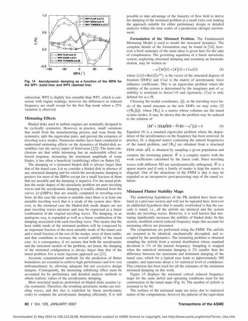
subsection. WP2 is slightly less unstable than WP1, which is con-sistent with engine readings, however the differences in reducedfrequency are small except for the first flap mode where a 25%variation is observed

Mistuning EffectsBladed disks used in turbine engines are nominally designed to

be cyclically symmetric. However, in practice, small variationsthat result from the manufacturing process and wear break thesymmetry, split the eigenvalue pairs, and prevent the existence oftraveling-wave modes. Numerous studies have been conducted tounderstand mistuning effects on the dynamics of bladed-disk as-semblies �see the survey paper of Srinivasan �22��. The main con-clusions are that while mistuning has an undesirable effect onforced response, increasing the maximum amplitude of someblades, it has often a beneficial �stabilizing� effect on flutter �6�.

The damping of a mistuned bladed disk is always larger thanthat of the tuned case. Let us consider a bladed disk in absence ofany structural damping and for which the aerodynamic damping ispositive for most of the IBPAs except for a small fraction of themthat are unstable and the damping is negative. For the tuned prob-lem the mode shapes of the aeroelastic problem are pure travelingwaves and the aerodynamic damping is readily obtained from thecurves = �IBPA� that are usually computed in traveling-waveform. In this case the system is unstable since there is at least oneunstable traveling wave that is a mode of the system also. How-ever, in the mistuned case the bladed-disk mode shapes are notpure traveling waves anymore and may be expressed as a linearcombination of the original traveling waves. The damping, in ananalogous way, is expanded as well as a linear combination of thedamping associated with each traveling wave. This means that theleast stable mode of the mistuned problem will be composed byan important fraction of the most unstable mode of the tuned caseand a small fraction of the rest of the modes, most of them stable,and that contribute to increase the overall stability of the tunedcase. As a consequence, if we assume that both the aerodynamicand the structural models of the problem, are linear, the dampingof the mistuned configuration is always larger than that of thetuned problem. For a more rigorous approach see �23�.

Accurate computational methods for the prediction of flutterboundaries are essential to achieve high performance and low costturbomachinery by allowing adequate but not excessive designmargins. Consequently, the mistuning stabilizing effect must beaccounted for by preliminary and detailed analysis methods toobtain realistic values of the aerodynamic damping.

Most structural analysis performed on bladed disks assume cy-clic symmetry. Therefore, the resulting aeroelastic modes are trav-eling waves, and this fact is exploited by linear aerodynamiccodes to compute the aerodynamic damping efficiently. It is still

possible to take advantage of the linearity of flow field to derivethe damping of the mistuned problem at a small extra cost makingthe approach suitable for either preliminary design or detailedanalyses within the time scales of a production �design� environ-ment.

Formulation of the Mistuned Problem. The FundamentalMistuning Model is used to model the structural dynamics. Thecomplete details of the formulation may be found in �24�, how-ever a brief summary of the main ideas is given here for the sakeof completeness. The governing equations of a linear aeroelasticsystem, neglecting structural damping and assuming an harmonicmotion, may be written as:

− �2�M��x + �K��x = C��x �8�

where �x�t� =Re��x ei�t�, is the vector of the structural degrees offreedom �DOFs� and C�� is the matrix of aerodynamic forceinfluence coefficients. This is an eigenvalue problem where thestability of the system is determined by the imaginary part of �;stability is restricted to Im��0 and rigorously, C�� is onlydefined for ��R.

Choosing the modal coordinates, �q , in the traveling wave ba-sis of the tuned structure as the new DOFs we may write �x = ��0��q , where ��0� is a matrix whose columns are the tunedsystem modes. It may be shown that the problem may be reducedto the solution of

��2 + 2�� − W�� − �2��q = 0 �9�Equation �9� is a standard eigenvalue problem where the depen-dence of the aerodynamics on the frequency has been removed. Inpractice, �, a diagonal matrix containing the natural frequenciesof the tuned problem, and ��0� are obtained from a structural

FEM while ��, is obtained by sampling a given population and

contains the mistuning pattern. W is a complex matrix with thework coefficients calculated by the linear code. Since traveling

waves with different ND are aerodynamically orthogonal, W is asparse matrix and if only a family of modes is kept the matrix isdiagonal. One of the attractions of the FMM is that it may beregarded as an inexpensive post-processing step of the tuned so-lution.

Mistuned Flutter Stability MapsThe underlying hypotheses of the PK method have been out-

lined in a previous section and will not be repeated here, howeveran additional hypothesis that is usually overlooked is that the cas-cade is tuned, i.e., all the airfoils are identical and the systemmodes are traveling waves. However, it is well known that mis-tuning significantly increases the stability of bladed disks. In thissection, modified critical reduced frequency maps that account formistuning effects are presented.

The computations are performed using the FMM. The airfoilsare assumed to be identical, mechanically decoupled, and re-coupled by the aerodynamics. The mistuning problem is obtainedsampling the airfoils from a normal distribution whose standarddeviation is 1% of the natural frequency. Sampling is stoppedwhen the statistical minimum damping is 2% smaller than thedifference between the maximum and minimum damping of thetuned case, which for a typical case leads to approximately 300samples, and represents about a 3� statistical level of confidence.This criterion has been used for all the estimates of the minimummistuned damping on this work.

Figure 15 displays the mistuned critical reduced frequencymaps for the same airfoil and operating conditions used for theconstruction of the tuned maps �Fig. 8�. The number of airfoils isassumed to be 84.

The isolines of the mistuned maps are noisy due to statisticalnature of the computations, however the patterns of the equivalent

Fig. 14 Aerodynamic damping as a function of the IBPA forthe WP1 „solid line… and WP2 „dashed line…



tuned maps �Fig. 8� are clearly recognized. The differences in thecritical reduced frequency with the tuned case are about 20% forthe freestanding airfoil, although this result is mode dependent.

For the welded-pair case �Fig. 15 �right��, airfoils are moved asa rigid body. The lower airfoil of the pair corresponds to thesection located at the bottom of row. The increase of the aerody-namic damping in all the modes with respect to the single bladeconfiguration is clearly seen. The pattern of both, the tuned �Fig. 8right�, and mistuned maps is similar, however in this case theeffect of mistuning is much higher than in the freestanding bladewith an increase of up to 30% in the reduced critical frequency forthe flap modes. Certainly, this is a factor that needs to be ac-counted for from an engineering point of view to produce mean-ingful results.

Mistuned Three-Dimensional ResultsThe methodology described in the previous section has been

applied to estimate the increase in aerodynamic damping due tomistuning in realistic bladed disks. The disk is assumed to beperfectly tuned while a normal population of blades with a stan-dard deviation, �, of 1% of the rotor blade natural frequency hasbeen used to perform a Monte Carlo simulation. The number ofdifferent bladed-disk samples per standard deviation is about 400,which represents about a 3� statistical level of confidence.

Figure 16 displays the minimum damping as a function of bladefrequency mistuning of the sample for the interlock configuration�solid symbols� and its equivalent welded pair �open symbols�.The horizontal lines represent the minimum damping for the tunedcase. It may be seen that the minimum of the tuned case and thatobtained with the Monte Carlo simulation are essentially the same

for the interlock configuration, not being the mistuning an effec-tive mechanism to increase the aerodynamic stability in this case.However, for the welded-in-pair rotor blades, the increment indamping is about 0.1%, which is comparable to the beneficialeffect of welding the airfoils in pairs.

The different sensitivity of the welded-pair and interlock con-figurations to mistuning is due to the different form of their fre-quency characteristics �see Fig. 12�. The minimum damping of theinterlock bladed disk occurs at low nodal diameters which areseparated modes and may not be effectively combined by mistun-ing, while the minimum damping for rotor blades welded in pairsoccurs in the high nodal diameter region, where many modes havenearly the same frequency and may be effectively combined bythe rotor blades’ mistuning to increase the minimum damping.

Figure 17 displays the damping as a function of the mistuningamplitude in frequency for the welded-pair equivalent of the in-terlock bladed disk. It may be seen that damping increases almostlinearly with the mistuning amplitude and then saturates for ��2%. The lower part of the envelope, that provides the minimumdamping, is the most relevant from an engineering point of view.The maximum damping saturates with the damping amplitude to avalue that approximately coincides with the mean damping of thefamily, while the minimum damping depends essentially on thestatistical confidence level.

Figure 18 shows the minimum damping as a function of thestandard deviation of the sample for the welded-pair bladed disksWP1 and WP2. WP1 is more unstable than WP2, as expected, andthe increase in damping due to mistuning effects is about 0.15%of the critical damping in both cases. This means that WP2 stillneeds about 0.2% of structural critical damping to become stable.

Fig. 15 Critical reduced frequency maps for mistuned freestanding „left… and welded-in-pair„right… airfoils

Fig. 16 Minimum damping as a function of the standard devia-tion of the rotor blade airfoil frequency for an interlock „solidsymbols… and a welded-pair „open symbols… blade disk

Fig. 17 Damping relative to the critical damping as a functionof the rotor blade frequency standard deviation



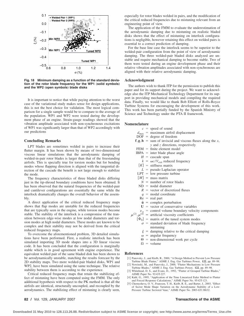
It is important to notice that while paying attention to the worstcase of the variational study makes sense for design applications,this is not the best choice for validation. The most logical com-parison for a single sample would be to compare to the average ofthe population. WP1 and WP2 were tested during the develop-ment phase of an engine. Strain-gauge readings showed that thevibration amplitude associated with non-synchronous excitationsof WP1 was significantly larger than that of WP2 accordingly withour predictions

Concluding RemarksLPT blades are sometimes welded in pairs to increase their

flutter margin. It has been shown by means of two-dimensionalviscous linear simulations that the aerodynamic damping ofwelded-in-pair rotor blades is larger than that of the freestandingairfoils. This is specially true for torsion modes but for bendingmodes whose flapping direction is aligned with the tangential di-rection of the cascade the benefit is not large enough to stabilizethe mode.

The frequency characteristics of three bladed disks differingjust in the tip-shroud boundary conditions have been obtained. Ithas been observed that the natural frequencies of the welded-pairand cantilever configurations are essentially the same while theinterlock dramatically changes the overall behavior of the assem-bly.

A direct application of the critical reduced frequency mapsshows that flap modes are unstable for the reduced frequenciesthat are typically seen in the engine, while torsion modes becomestable. The stability of the interlock is a compromise of the tran-sition between edge-wise modes at low nodal diameters and tor-sion modes at high nodal diameters. These modes are known to becomplex and their stability may not be derived from the criticalreduced frequency maps.

To overcome the aforementioned problem, 3D detailed simula-tions have been performed. First, a realistic interlock has beensimulated importing 3D mode shapes into a 3D linear viscouscode. It has been concluded that the configuration is marginallystable which is in good agreement with engine experience. Theequivalent welded pair of the same bladed disk has been shown tobe aerodynamically unstable, matching the results forecast by the2D stability maps. Two more welded-pair bladed disks, WP1 andWP2, have been simulated using the same technique. The relativestability between them is according to the experience.

Critical reduced frequency maps that retain the stabilizing ef-fect of mistuning have been computed using the FMM. The onlyadditional hypothesis with respect to the PK method is that all theairfoils are identical, structurally uncoupled, and recoupled by theaerodynamics. The stabilizing effect of mistuning is clearly seen,

especially for rotor blades welded in pairs, and the modification ofthe critical reduced frequencies due to mistuning relevant from anengineering point of view.

The application of the FMM to evaluate the underestimation ofthe aerodynamic damping due to mistuning on realistic bladeddisks shows that the effect of mistuning on interlock configura-tions is negligible, however retaining this effect on welded pairs isessential to a correct prediction of damping.

For the base line case the interlock seems to be superior to thewelded-pair configuration from the point of view of aerodynamicdamping. The three welded-pair bladed disks analyzed are un-stable and require mechanical damping to become stable. Two ofthem were tested during an engine development phase and theirrelative vibration amplitudes associated with non-synchronous arealigned with their relative aerodynamic damping.

AcknowledgmentThe authors wish to thank ITP for the permission to publish this

paper and for its support during the project. We want to acknowl-edge also the ITP Mechanical Technology Department for its sup-port in providing mechanical models and compiling the requireddata. Finally, we would like to thank Bob Elliott of Rolls-RoyceTurbine Systems for encouraging the development of this work.This work has been partially funded by the Spanish Ministry ofScience and Technology under the PTA II framework.

Nomenclaturec � speed of sound

dmax � maximum airfoil displacementDOF � degree of freedom

f ,g ,h � sum of inviscid and viscous fluxes along the x,y and z directions, respectively

FEM � finite element modelIBPA � inter blade phase angle

H � cascade spank � �c /Vexit reduced frequency

�K� � stiffness matrixL � pseudo Laplacian operator

LPT � low pressure turbine�M� � mass matrix

N � number of rotor bladesND � nodal diameter

R � vector of discretized fluxesq � modal coordinate

Re � real partu � complex perturbationU � vector of conservative variablesv� � control volume boundary velocity components

��2� ,��4� � artificial viscosity coefficients��0� � matrix of the tuned system modes

� � standard deviation of blade frequencymistuning

� damping relative to the critical damping� � angular frequency � non-dimensional work per cycle� � volume

References�1� Panovsky, J., and Kielb, R., 2000, “A Design Method to Prevent Low Pressure

Turbine Blade Flutter,” ASME J. Eng. Gas Turbines Power, 122, pp. 89–98.�2� Nowinski, M., and Panovsky, J., 2000, “Flutter Mechanisms in Low Pressure

Turbine Blades,” ASME J. Eng. Gas Turbines Power, 122, pp. 89–98.�3� Whitehead, D. S., and Evans, D., 1992, “Flutter of Grouped Turbine Blades,”

ASME Paper No. 92-GT-227.�4� Kahl, G., 1995, “Application of the Time Linearized Euler Method to Flutter

and Forced Response Calculations,” ASME Paper No. 95-GT-123.�5� Chernysheva, O. V., Fransson, T. H., Kielb, R. E., and Barter, J., 2003, “Effect

of Sector Mode Shape Variation on the Aerodynamic Stability of a Low-Pressure Turbine Sectored Vane,” ASME Paper No. 2003-GT-38632.

Fig. 18 Minimum damping as a function of the standard devia-tion of the rotor blade frequency for the WP1 „solid symbols…and the WP2 „open symbols… blade disks



�6� Kaza, K.-R. V., and Kielb, R. E., 1982, “Flutter and Response of a MistunedCascade in Incompressible Flow,” AIAA J., 20�8�, pp. 1120–1127.

�7� Bendiksen, O. O., 1984, “Flutter of Mistuned Turbomachinery Rotors,” ASMEJ. Eng. Gas Turbines Power, 106, pp. 25–33.

�8� Crawley, E., 1987, Manual on Aeroelasticity in Axial Flow TurbomachinesVol. 2, Structural Dynamics and Aeroelasticity, Chapter on Aeroelastic Formu-lation of Tuned and Mistuned Rotor, pp. 19-1–19-24.

�9� Sadeghi, M., and Liu, F., 2001, “Computation of Mistuning Effects on CascadeFlutter,” AIAA J., 39�1�, pp. 22–28.

�10� Seinturier, E., Dupont, C., Berthillier, M., and Dumas, M., 2002, “A NewMethod to Predict Flutter in Presence of Structural Mistuning With Applicationto a Wide Chord Fan Stage,” 9th International Symposium on Unsteady Aero-dynamics, Aeroacoustics and Aeroelasticity of Turbomachines, P. Ferrand, ed.,Lyon, France, September, pp. 739–749.

�11� Sommer, T. P., Stanppenbeck, F., and Schmitz, M., 2002, “Application ofProbabilistic Design Methods to the Prediction of Turbomachinery Blade Flut-ter,” 9th International Symposium on Unsteady Aerodynamics, Aeroacousticsand Aeroelasticity of Turbomachines, P. Ferrand, ed., Lyon, France, September,pp. 387–396.

�12� Corral, R., Escribano, A., Gisbert, F., Serrano, A., and Vasco, C., 2003, “Vali-dation of a Linear Multigrid Accelerated Unstructured Navier-Stokes Solverfor the Computation of Turbine Blades on Hybrid Grids,” AIAA Paper No.2003-3326.

�13� Corral, R., Crespo, J., and Gisbert, F., 2004, “Parallel Multigrid UnstructuredMethod for the Solution of the Navier-Stokes Equations,” AIAA Paper No.2004-0761.

�14� Jameson, A., Schmidt, W., and Turkel, E., 1981, “Numerical Solution of the

Euler Equations by Finite Volume Techniques Using Runge-Kutta Time Step-ping Schemes,” AIAA Paper No. 81-1259.

�15� Roe, P., 1981, “Approximate Riemman Solvers, Parameters, Vectors and Dif-ference Schemes,” J. Comput. Phys., 43, pp. 357–372.

�16� Swanson, R. C. and Turkel, E., 1992, “On Central-Difference and UpwindingSchemes,” J. Comput. Phys., 101, pp. 292–306.

�17� Corral, R., Burgos, M. A., and Garcia, A., 2000, “Influence of the ArtificialDissipation Model on the Propagation of Acoustic and Entropy Waves,”ASME Paper No. 2000-GT-563.

�18� Baldwin, B. S., and Lomax, H., 1978, “Thin Layer Approximation and Alge-braic Model for Separated Flows,” AIAA Paper No. 78-257.

�19� Giles, M. B., 1990, “Non-Reflecting Boundary Conditions for Euler EquationCalculations,” AIAA J., 28�12�, pp. 2050–2057.

�20� Corral, R., and Gisbert, F., 2003, “A Numerical Investigation on the Influenceof Lateral Boundaries in Linear Vibrating Cascades,” ASME J. Turbomach.,125, pp. 433–441.

�21� Sayma, A. I., Vahdati, M., Green, J. S., and Imregun, M., 1998, “Whole-Assembly Flutter Analysis of a Low Pressure Turbine Blade,” 8th Interna-tional Symposium on Unsteady Aerodynamics and Aeroelasticity of Turboma-chines, T. Fransson, ed., Stokholm, Sweden, pp. 347–359.

�22� Srinivasan, A. V., 1984, “Vibrations of Bladed-Disc Assemblies-A SelectedSurvey,” ASME J. Vib., Acoust., Stress, Reliab. Des., 106�2�, pp. 165–168.

�23� Martel, C., Corral, R., and Llorens, J. M., 2006, “Stability Increase of Aero-dynamically Unstable Rotors Using Intentional Mistuning,” ASME Paper No.2006-GT-90407.

�24� Feiner, D. M., and Griffin, J. H., 2002, “A Fundamental Model of Mistuningfor a Single Family of Modes,” ASME J. Turbomach., 124, pp. 597–605.



Steven J. ThorpeDepartment of Aeronautical and Automotive

Engineering,Loughborough University,

Loughborough LE12 7TW, UKe-mail: [email protected]

Robert J. MillerWhittle Laboratory,

University of Cambridge,Cambridge CB3 0DY, UK

Shin YoshinoTokyo Electric Power Company,

Yokohama 230-8510, Japan

Roger W. AinsworthDepartment of Engineering Science,

University of Oxford,Oxford OX1 3PJ, UK

Neil W. HarveyRolls-Royce plc,

Derby DE24 8BJ, UK

The Effect of Work Processeson the Casing Heat Transferof a Transonic TurbineThis paper considers the effect of the rotor tip on the casing heat load of a transonic axialflow turbine. The aim of the research is to understand the dominant causes of casing heattransfer. Experimental measurements were conducted at engine-representative Machnumber, Reynolds number, and stage inlet to casing wall temperature ratio. Time-resolvedheat-transfer coefficient and gas recovery temperature on the casing were measuredusing an array of heat-transfer gauges. Time-resolved static pressure on the casing wallwas measured using Kulite pressure transducers. Time-resolved numerical simulationswere undertaken to aid understanding of the mechanism responsible for casing heat load.The results show that between 35% and 60% axial chord the rotor tip-leakage flow isresponsible for more than 50% of casing heat transfer. The effects of both gas recoverytemperature and heat transfer coefficient were investigated separately and it is shownthat an increased stagnation temperature in the rotor tip gap dominates casing heattransfer. In the tip gap the stagnation temperature is shown to rise above that found atstage inlet (combustor exit) by as much as 35% of stage total temperature drop. The risein stagnation temperature is caused by an isentropic work input to the tip-leakage fluid bythe rotor. The size of this mechanism is investigated by computationally tracking fluidpath lines through the rotor tip gap to understand the unsteady work processes thatoccur. �DOI: 10.1115/1.2372772�

Winner of the Turbo Expo Heat Transfer Committee Best Paper Award

IntroductionThe blade-tip region of a high-pressure turbine continues to

present a challenge to gas turbine engine manufacturers due to thecomplex aerothermal conditions encountered in this region of themachine. High flow temperatures, unsteady blade row interactionsand cooling difficulties have resulted in a situation where design-ers rely on expensive design phase iterations rather than an appro-priate physical understanding of the flow and heat transfer �1�.There is of course a desire to increase turbine entry temperaturesstill further, and this means that an improved knowledge of theflow physics in this area will continue to be important for theforeseeable future. Many investigations of blade-tip aerodynamicsand heat transfer have been conducted in an attempt to providedesigners with a good physical understanding of how flow phe-nomena affect blade-tip heat transfer and tip-leakage loss. Thevast majority of this work has been performed in low-speed testfacilities, usually in the form of linear cascades with no relativemotion between blade and casing wall. These tests have beenessential in gaining an appreciation of the general features of theflow field in the region of the blade tip gap.

By comparison far less work has been reported on the aerody-namic and heat transfer aspects of the stationary overtip casingwall. This component is itself exposed to fierce convective heattransfer and requires careful cooling system design. At present,the knowledge of the relationship between the blade row aerody-namics and the casing heat transfer is poor. This paper will showthat it is important to consider the turbine as an aerothermal ma-chine, and that the transfer of work within the turbine causes

spatial and temporal distributions of total temperature that arecritical to understanding the origins of the heat load to which theovertip casing is subjected.

Historical PerspectiveA large body of literature is available relating to the overtip

leakage problem in high-pressure turbines, see, for example, Ref.�2�. Indeed, the basic physical process by which the pressure dif-ference across the blade tip drives a leakage of fluid from pressuresurface to suction surface is well understood from low-speed cas-cade experimentation, as is the interaction of this leakage fluidwith the blade passage flow �producing the tip-leakage vortex,e.g., Ref. �3��. Detailed measurements of the effect of blade-tiptreatments and tip-gap height have been reported by several work-ers, including Heyes et al. �4� for a low-speed cascade with tipclearance. These investigations are typically concerned with theimpact of tip leakage on the aerodynamic loss in the turbine. Theexperimental investigation of heat transfer in the tip region hasbeen less widely reported in the open literature, although an in-crease in activity has been apparent in recent years. In addition,the available literature concentrates on the heat transfer to turbineblade tips rather than overtip casing, with the work of Kim andMetzger �5�, Papa et al. �6�, and Srinivasan and Goldstein �7�being representative examples. The findings of these and otherworkers are important for establishing the effects of tip-gapheight, tip geometry, and blade/casing relative motion.

Moore et al. �8� highlighted the inadequacy of low-speed facili-ties in simulating the true flow structure in the tip gap. This is dueto the pressure ratio across a high-pressure blade tip being suffi-cient to accelerate the flow to supersonic Mach numbers. Thepublished literature contains only a small quantity of experimentalinformation that has been obtained at fully representative flowconditions for the high-speed axial turbine. The first report ofovertip casing heat transfer and aerodynamics for a fully scaledtransonic turbine stage was by Guenette et al. �9�, who showed the

Contributed by the International Gas Turbine Institute �IGTI� of ASME for pub-lication in the JOURNAL OF TURBOMACHINERY. Manuscript received October 1, 2004;final manuscript received February 1, 2005. IGTI Review Chair: K. C. Hall. Paperpresented at the ASME Turbo Expo 2005: Land, Sea and Air, Reno, NV, June 6–9,2005, Paper No. GT2005-68437.



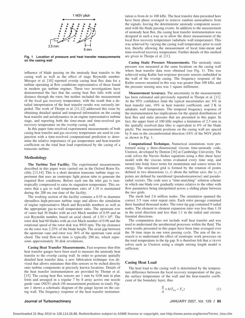
influence of blade passing on the unsteady heat transfer to thecasing wall as well as the effect of stage Reynolds number.Metzger et al. �10� reported overtip casing heat flux data for aturbine operating at flow conditions representative of those foundin modern gas turbine engines. These two investigations havedemonstrated the fact that the casing heat flux falls with axialdistance through the rotor, but neither included the measurementof the local gas recovery temperature, with the result that a de-tailed interpretation of the heat transfer results was seriously im-peded. The work of Thorpe et al. �11,12� addressed this issue byobtaining detailed spatial and temporal information on the casingheat transfer and aerodynamics in an engine representative turbinestage, and reporting both the time-mean and time-resolved gasrecovery temperature on the overtip casing wall.

In this paper time-resolved experimental measurements of bothcasing heat transfer and gas recovery temperature are used in con-junction with a time-resolved computational prediction to deter-mine the relative importance of gas temperature and heat-transfercoefficient on the total heat load experienced by the casing of atransonic turbine.

Methodology

The Turbine Test Facility. The experimental measurementsdescribed in this paper were carried out in the Oxford Rotor Fa-cility �13,14�. This is a short duration transonic turbine stage ex-periment that uses an isentropic light piston tube to generate therequired flow conditions. Before each run the inlet gas is isen-tropically compressed to raise its stagnation temperature. This en-sures that a gas to wall temperature ratio of 1.18 is maintainedduring the 200 ms run time of the facility.

The working section of the facility contains a 0.55 m diametershroudless high-pressure turbine stage and allows the simulationof engine representative Mach and Reynolds numbers as well asthe appropriate gas-to-wall temperature ratio. The upstream rowof vanes had 36 blades with an exit Mach number of 0.95 and anexit Reynolds number, based on axial chord, of 1.55�106. Therotor disk had 60 blades with an exit Mach number of 0.98 and therotational speed of the rotor disk was 8910 rpm. The tip clearanceon the rotor was 2.25% of the blade height. The axial gap betweenthe upstream vane and rotor was 36% of the upstream vane axialchord. The total flow-on time is typically 200 ms, which repre-sents approximately 30 disk revolutions.

Casing Heat Transfer Measurements. Fast-response thin-filmheat transfer gauges have been used to measure the unsteady heattransfer to the overtip casing wall. In order to generate spatiallydetailed heat transfer data, a new fabrication technique was de-vised that allows miniature thin-film sensors to be etched directlyonto turbine components at precisely known locations. Details ofthe heat transfer instrumentation are provided by Thorpe et al.�15�. The casing heat flux sensors are 1 mm by 0.08 mm in planform and arranged in a regular 7 by 8 array across one nozzleguide vane �NGV� pitch �56 measurement positions in total�. Fig-ure 1 shows a schematic diagram of the gauge layout on the cas-ing wall. The frequency response of the heat transfer instrumen-

tation is from dc to 100 kHz. The heat transfer data presented herehave been phase averaged to remove random unsteadiness fromthe signals, leaving the deterministic unsteady component associ-ated with the blade passing events. In addition to the measurementof unsteady heat flux, the casing heat transfer instrumentation wasdesigned in such a way as to allow the direct measurement of thelocal flow recovery temperature �adiabatic wall temperature�. Thiswas achieved by varying the casing wall temperature prior to eachtest, thereby allowing the measurement of local time-mean andtime-resolved recovery temperature. Further details of this methodare given in Thorpe et al. �11�.

Casing Static Pressure Measurements. The unsteady staticpressure was measured at the same locations on the casing wallwhere heat transfer data were obtained �see Fig. 1�. This wasachieved using Kulite fast-response pressure sensors embedded inthe wall of the overtip casing. The frequency response of theKulite sensors mounted in this way was greater than 100 kHz, andthe pressure sensing area was 1 square millimeter.

Measurement Accuracy. The uncertainty in the measurementshas been estimated and previously reported in Thorpe et al. �11�.At the 95% confidence limit the typical uncertainties are: 6% inheat transfer rate, 10% in heat transfer coefficient, and 2 K inadiabatic wall temperature. The temporal frequency response ofthe instrumentation has implications for the spatial distributions ofheat flux and static pressure that are presented in this paper. Infact, the upper limit of 100 kHz implies a limitation of 2.5 mm inthe spatially resolved data �this is equivalent to 6% of the bladepitch�. The measurement positions on the casing wall are spacedby 8 mm in the circumferential direction �16% of the NGV pitch�as shown in Fig. 1.

Computational Technique. Numerical simulations were per-formed using a three-dimensional viscous time-unsteady code,Unstrest, developed by Denton �16� at Cambridge University. Thecode solves the Navier–Stokes equations using a thin shear layermodel with the viscous terms evaluated every time step, andturned into body force terms for momentum and source terms forenergy. The structured grid is formed by the rotation of pointsdefined in two dimensions �x ,r� about the turbine axis; the �x ,r�points are defined by meridional �pseudostreamwise� and pseudo-radial vectors. The code uses a “time-marching” solution schemein which one blade row gradually rotates relative to the other withflow parameters being interpolated across a sliding plane betweenthe two grids.

The mesh had 2.6 million nodes. The simulation spanned thecorrect 3:5 vane rotor repeat ratio. Each rotor passage containedthree hundred thousand nodes. The rotor tip gap contained 9 radialnodes. The element to element expansion ratio was less than 1.18in the axial direction and less than 1.1 in the radial and circum-ferential directions.

The computation does not include wall heat transfer and wasused to understand the aerothermal processes within the fluid. Therotor results presented in this paper have been time averaged overthe 36 time steps in one rotor passing cycle. The aim of the re-search is to understand the effect of isentropic work processes onthe total temperature in the tip gap. It is therefore felt that a URANS

solver such as Unstrest using a simple mixing length model issufficient.

Casing Heat LoadThe heat load to the casing wall is determined by the tempera-

ture difference between the local recovery temperature of the gas,the surface temperature of the wall and the heat-transfer coeffi-cient of the boundary layer, thus

q

A= h�Trec − Tw� �1�

Fig. 1 Location of pressure and heat transfer measurementson the casing wall



Using the stage inlet total temperature this can be rearranged togive

q

T0A= h�Trec

T0−

Tw

T0� �2�

If in a particular turbine the boundary layer heat-transfer coef-ficient �h� and the gas recovery temperature �Trec� are known thento calculate heat transfer rate �q� it is necessary to specify thestage inlet to wall temperature ratio �T0 /Tw�. In an optimized gasturbine design the casing would require the minimum level ofcooling possible. This would mean that its surface would be de-signed to run at the maximum allowable temperature of the par-ticular material used. If the casing were covered in a thermalbarrier coating, with a maximum surface temperature stipulated tobe 1500 K, the casing surface temperature would be designed tobe 1500 K at all axial locations. As the gas passes through therotor work is extracted and its stagnation temperature drops. Thiscauses the driving temperature difference �Trec−Tw� to fall fromrotor leading edge to trailing edge. The cooling on such an ideal-ized turbine would be optimized to take advantage of this axialreduction in heat transfer, with the casing towards the trailingedge requiring less cooling air than at the leading edge.

For a modern civil aeroengine with a turbine entry temperatureof 1800 K and a casing that employs a thermal barrier coating, thestage inlet to wall temperature ratio is 1.2. For the testing reportedin this paper the stage inlet to wall temperature ratio was set at1.18.

The aim of this section is to determine the spatial and temporaleffect of the rotor on the casing heat load. Equation �1� will thenbe used to determine the relative importance of gas temperatureand heat-transfer coefficient on the heat load.

Spatial Distribution of Heat Load. An instantaneous snap-shot of the experimentally measured casing heat transfer rate isshown in Fig. 2. The measurements show strong spatial variationsboth circumferentially and axially, and very high levels of casingheat transfer are observed within the blade-tip footprint. The high-est values occur in the vicinity of the crown of the blade andtoward the blade suction surface. A region of elevated heat trans-fer is also seen axially forward of the blade tips in the vane-rotoraxial gap. The pattern of casing heat load shown in Fig. 2 movesat blade speed relative to the casing wall; consequently, a fixedpoint on the casing wall is alternately exposed to blade passageflow and blade tip leakage flow. This can be appreciated from the

schematic diagram at the top of Fig. 2.The total heat load at any particular point on the casing wall can

be divided into portions that originate from either the rotor pas-

sage flow or the rotor tip flow: these are shown as QB and QArespectively in Fig. 2. To quantify the fraction of casing heat loadthat is caused by the presence of an individual rotor tip the totalheat transfer at each measurement point has been split into theheat transfer above a rotor tip and above the passage flow �usingthe time-resolved data�. The axial variation of each of these com-ponents is shown in Fig. 3. The measurements show that eventhough the rotor-tip covers only between 10% and 24% of thecasing circumference �depending on axial position� it contributesup to 50% of the total heat load to the casing. Figure 2 shows thatin addition to the enhanced heat transfer above the rotor the pres-ence of the rotor also enhances heat transfer close to the suctionsurface, pressure surface, and upstream of the blade. The totalcontribution of the rotor-tip to casing heat load can therefore bewell over 50%.

Cause of High Heat Load Above the Rotor. Equation �1�shows that a high casing heat load above the rotor can be causedby: �1� an elevated gas temperature ratio �Trec /T0�; �2� an elevatedheat transfer coefficient �h�; or �3� a combination of the two. Theaxial variation of gas temperature ratio and heat transfer coeffi-cient derived from the experimental results is shown in Figs. 4 and5 �these data represent average values for tip and passageregions�.

Figure 4 shows the circumferentially and temporally averagedgas recovery temperature over the rotor tip and passage flow. Themaximum difference between the passage and tip stagnation tem-peratures occurs at 50% axial chord and shows an 11% rise. It isinteresting to note that this rise in stagnation temperature is 40%

Fig. 2 Time-resolved measurements of the casing heat trans-fer rate

Fig. 3 Experimentally measured casing heat load caused byrotor tip and passage flows

Fig. 4 Experimentally measured casing recovery temperaturein the rotor tip gap and rotor passage



of the total stagnation temperature drop across the stage. The in-crease in casing heat transfer rate caused by the temperature riseabove the rotor tip can be found from Eq. �1�. The stage inlet towall stagnation temperature ratio �T0 /Tw� in the Oxford RotorFacility is 1.18. The 11% rise in stagnation temperature thuscauses a 250% rise in heat transfer.

The maximum measured difference between the passage and tipheat transfer coefficient occurs at 35% axial chord �Fig. 5�. At thislocation the casing heat transfer coefficient in the rotor tip gap is55% higher than in the blade passage. Table 1 shows the increasein casing heat load caused by the rotor tip flow at 50% axialchord. The results show that at a stage inlet to wall temperatureratio of 1.2 �typical of a civil aeroengine� the heat transfer rises bya factor of 2.09 compared to the case when the tip-leakage flow isnot present. It is important to note that the reason the temperaturevariation has such a large effect on casing heat load is that thepeak temperature in the tip gap was measured to be 35% of stage�T0 above the stage inlet temperature. If an overtip casing isdesigned to have a stage inlet to wall temperature ratio �T0 /Tw� of1.2 the driver temperature at 50% axial chord is only 15% of stage�T0. Table 1 also shows the effect of raising T0 /Tw to 1.4. This isequivalent to increasing casing cooling until the wall surface tem-perature is limited to 1286 K. At these wall temperatures the ef-fects of stagnation temperature and heat transfer coefficient have acomparable effect on the casing heat load.

Time-Resolved Casing Wall Temperature. Figure 6 shows themeasured distribution of time-resolved gas recovery temperaturefor the same instant in the blade passing cycle as the heat transferrate data shown in Fig. 2. Figure 7 shows the comparable compu-tational results averaged over one vane passing cycle. Upstream ofthe blade row the recovery temperature on the casing wall is highand close to the stage inlet total temperature of 374 K. The rotorpotential field causes a stagnation temperature variation upstreamof the blade. Within the rotor passage the flow recovery tempera-ture falls as work is extracted from the fluid.

Over the rotor tip the gas recovery temperatures rise above thestage inlet stagnation temperature. In both the experiment andcomputation the region of highest temperature rise occurs on the

suction side of the blade tip. The highest measured stagnationtemperature was 35 K above that at stage inlet �35% stage �T0�.The highest computationally predicted stagnation temperature was40 K above stage inlet.

The results in this section have shown that at engine represen-tative stage inlet to wall temperature ratios the presence of therotor tip leakage can double the local heat load. This rise in heatload is caused by the recovery temperature of the gas in the rotortip gap reaching values 35% of stage �T0 above stage inlet andenhanced levels of heat transfer coefficient. The following sectionexplains the mechanism for this rise.

Effect of Work ProcessesThe change in the stagnation enthalpy and temperature of a

fluid particle per unit time and mass, in a particular frame ofreference, is given by

Dh0

Dt=

1

�

�qi

�xi+

1

�

��ijui��xj

+1

�

�p

�t�3�

Fig. 5 Experimentally measured casing heat transfer coeffi-cient in the rotor tip gap and rotor passage

Table 1 Increase in casing heat load caused by elevated levelsof h and Trec in the rotor tip gap at 50% axial chord „expressedas a factor relative to the no tip-leakage case…

T0 /Tw 1.2 1.4Effect of h 1.09 1.09

Effect of Trec /T0 1.68 1.13Total rise in Q 2.09 1.29

Fig. 6 Measurement of the time-resolved gas recovery tem-perature on the casing wall

Fig. 7 Time-mean computational prediction of casing flow to-tal temperature



The three source terms are the heat flow into the element, thework done by viscous stresses, and the change in enthalpy causedby temporal gradients in the static pressure field. The stagnationtemperature of a gas is altered by the frame of reference in whichit is viewed. If the flow through the rotor gap is observed in therotor relative frame the problem becomes steady and the thirdterm in Eq. �3� does not occur. The heat transfer to the casing wallis driven by the stagnation temperature in the casing �stationary�frame of reference. In the stationary frame the rotor flow is un-steady and thus the third term in Eq. �3� is nonzero.

To understand the possible causes of the rise in stagnation tem-perature of the fluid as it passes into the rotor tip gap it is worthexamining the source terms on the right of Eq. �3�.

The first term represents the net heat transfer into or out of thefluid. This can be caused either by conduction of heat through thefluid or by the mixing of the fluid with a second stream of differ-ing temperature. Heat transfer to a fluid particle can only occurfrom a hotter source. The temperatures in the rotor tip gap arehigher than at combustor exit. Heat transfer therefore cannot bethe cause of the elevated tip temperatures.

The second term represents viscous work done on or by thefluid. In the stationary frame of reference the casing wall is notmoving and therefore cannot do viscous work on the fluid. Therotor tip moves in the direction of fluid motion with a velocity lessthan that of the fluid. This results in the rotor tip applying a vis-cous drag to the fluid. The rotor’s viscous drag extracts work fromthe fluid causing a drop in its stagnation enthalpy.

The third term shows that in an isentropic fluid the stagnationenthalpy can only be changed by the presence of a temporal varia-tion in static pressure at a stationary point in the chosen frame ofRef. �17�. It should be noted that the drop in stagnation tempera-ture of the core fluid as it moves through the rotor �isentropicwork extraction� is as a result of the movement of the rotor staticpressure field relative to the stationary frame. For the stagnationenthalpy in the casing frame of reference to rise as a fluid particleenters the tip gap the fluid must therefore experience a positivetemporal static pressure gradient.

Casing Static Pressure. The unsteady pressure field at a fixedpoint in space is the result of the movement of the rotor pressurefield at blade speed. The computationally predicted and experi-mentally measured static pressure fields on the casing wall areshown in Figs. 8 and 9. The computational and experimental re-sults exhibit a number of similar features. A band of low staticpressure stretches from around 50% axial chord to the trailingedge on the suction side of the gap �marker A�. This is caused bythe overexpansion of fluid to supersonic Mach numbers in the tipgap. The casing passage boundary layer migrates under the influ-ence both of the relative wall motion and the cross-passage pres-sure gradient towards the rotor suction surface. Where the casing

boundary layer meets the rotor tip-leakage jet the flow separatesfrom the casing wall and the tip-leakage flow rolls up into a vor-tical type structure �“tip-leakage vortex”�. This causes the staticpressure close to the rotor suction surface first to rise �marker B�then to fall �marker C�. The structure of the static pressure fielddescribed above is characteristic of shroudless transonic turbines.The temporal static pressure gradient in the stationary frame ofreference is obtained by moving the static pressure field �Fig. 8� atthe blade speed and at each point differentiating with respect totime. The temporal static pressure gradient is shown in Fig. 10. Anumber of distinct regions are observed. Marker D shows thenegative temporal pressure gradient in the rotor passage causing

Fig. 8 Time-mean computational prediction of casing staticpressure

Fig. 9 Experimental measurements of the time-resolved cas-ing static pressure

Fig. 10 Computationally predicted temporal gradient in staticpressure and experimentally measured pressure



work extraction in the main passage. Marker E shows the accel-eration of fluid through the tip gap causing a positive temporalpressure gradient and thus work addition. Marker F shows that asthe fluid leaves the tip gap it experiences a negative temporalpressure gradient and thus a work extraction. Marker G shows thatthe tip leakage vortex results in work extraction and additiondownstream of the blade trailing edge.

The bottom half of Fig. 10 shows the experimentally measuredstatic pressure at locations 5 and 7. The gauges show the twodistinct regions of the tip flow. Upstream of 50% Cax �gauge 5�the pressure on the casing wall first rises then is observed to fall.This indicates that the flow accelerates in to the gap then starts tomix within the gap. It should be noted that the temporal band-width of the pressure measurements is 100 kHz and this limits theminimum measurable spatial frequency �Fig. 10�. This makes ob-servation of small flow structures such as the pressure surfaceseparation bubble impossible. Downstream of 50% Cax �gauge 7�the pressure on the casing wall drops throughout the gap. Thisindicates that the flow continues to accelerate to the exit of thegap.

Enthalpy Change Along Rotor Relative Path Lines. To de-termine the effect of temporal pressure gradients on the stagnationenthalpy of the tip flow it is necessary to track fluid particles asthey travel along path lines through the rotor tip gap. Fluid pathlines are frame independent and represent the path along whichthe fluid particles travel. Figure 11 shows seven path lines thatpass through the rotor tip gap. For simplicity the path lines werestarted at time zero at points located at the midradius and midcir-cumference of the tip gap. The axial locations of the points wereequispaced between the rotor leading edge and trailing edge. Thepath lines were then tracked for both positive and negative timeuntil they left the domain. It should be noted that path-lines andstreamlines coincide in steady flow. Figure 11 can thus be inter-preted as streamlines in the rotor-relative frame.

The stagnation temperature variation along the seven path linesis shown in Fig. 12. The path lines are plotted above each otherwith the stage inlet stagnation temperature for each, plotted as adotted line �Note that the stage inlet stagnation condition is thesame for all path lines.�. The time at which the path line enters andleaves the tip gap are marked with circles.

The change in swirl velocity of a fluid particle in an inviscidflow is given by

Dr��

Dt= −

r

�

�p

r��

If the flow in the rotor is considered steady in the rotor-relativeframe then the spatial pressure gradient in the rotor can be relatedto the temporal pressure gradient such that

Dr��

Dt= −

1

�

�p

��=

1

��

�p

�t

Combining the above with the isentropic form of Eq. �3� andintegrating from a point at rotor inlet to a point on the same pathline gives

�hois =�1

21

�

�p

�tdt = u2��2 − u1��1 �4�

The above equation shows that the change in isentropic stagna-tion temperature of a fluid particle travelling through the rotor caneither be obtained by integrating the temporal pressure gradientalong a path line or from the Euler work equation. Both methodsof calculating the stagnation temperature along a path line areshown in Fig. 12.

The total temperature calculated from the Euler work equationfor a particle is shown as a dotted line in Fig. 12. It should benoted that a constant radius was assumed in the calculation of theblade velocity. This causes a small error downstream of the rotortip gap. It should also be noted that the total temperature predictedby the Euler equation agrees closely with that predicted by theviscous computation. The derivation of the Euler equation for a

Fig. 11 Fluid path lines through the rotor tip gap

Fig. 12 Computationally predicted stagnation temperaturevariations along seven path lines „these path lines are shownin Fig. 11…



particle, given above, is for an isentropic flow. Figure 12 indicatesthat it accurately predicts the total temperature variation in theviscous flow.

The total temperature change derived by integration of the tem-poral pressure field agrees well with the numerical prediction upto the exit of the tip gap. Downstream of the exit of the gap thetotal temperature is over estimated. Equation �4� shows that theintegral of the temporal pressure gradient gives only the isentropicchange in total enthalpy. The difference between the two tempera-tures is a result both of viscous processes in the rotor relativeframe and of the limited accuracy of the path-line tracking aroundthe core of the tip vortex.

The seven path lines fall into two groups. The first group lo-cated downstream of 50% Cax �path lines E, F, G� have a low gaplength to height ratio �between 4 and 1�. As shown in Fig. 10 thisresults in acceleration of the fluid throughout the gap and thus awork addition throughout. This shows that the stagnation tempera-ture is raised by up to 80 K by work addition. The second grouplocated upstream of 50% Cax �path lines A, B, C, and D� has ahigh gap length to height ratio �between 12 and 5�. In this regionthe tip-leakage flow experiences both a positive temporal pressuregradient as it accelerates into the gap and a negative temporalpressure gradient as it mixes within the gap. On path lines A andB the isentropic work addition over predicts the total temperaturewithin the gap. This is likely to be caused by the viscous processesin the rotor relative frame.

The above discussion shows that the majority of the rise instagnation temperature over the tip gap results from isentropicwork input from the rotor. In this way the rotor tip gap can beviewed as a super high-pressure compressor stage.

Design ImplicationsThe area of the casing wall affected by the highest stagnation

temperature is dependent on the geometry of the rotor tips. If asingle squealer tip as used on the suction surface then the stagna-tion temperature rise would only occur for a very small percentageof the circumference, lowering the total casing heat load. This isbecause as soon as the fluid re-entered the mainstream work ex-traction occurs and the casing boundary layer would cause thetip-leakage fluid to leave the casing wall. If a single squealer tipwas used on the pressure surface the opposite would occur and theregion of stagnation temperature would be maximized raising thetotal casing heat load.

It should be noted that low-speed testing does not correctlysimulate the magnitude of the work processes in the rotor. Thismeans that in a low-speed test the gas temperature through therotor tip gap will remain constant and the casing heat load will beunderestimated. The results from low-speed tests should thereforebe compensated for variations of gas temperature caused by workprocesses.

ConclusionsThe experimental results show the presence of the rotor tip

causes large spatial and temporal variations in instantaneous heatflux to the overtip casing wall. Analysis of the time resolved datahas shown that over half of the local heat load to the casing wallcan be attributed to the tip-leakage fluid. The experimental resultsallow the individual effects of gas recovery temperature and heattransfer coefficient to be investigated. For an axial turbine with astage inlet to wall temperature ratio of 1.2 the rise in stagnationtemperature caused by the rotor tip leakage flow results in a 68%increase in the heat load at 50% axial chord. The rise in heat loaddue to increased heat transfer coefficient at the same location is9%.

The computation and experiment show the stagnation tempera-ture in the tip gap rising by 40% and 35% of stage �T0. Themajority of this change is caused by an isentropic work addition to

the flow within the tip gap. The maximum calculated stagnationtemperature rise was found to be 80 K. On leaving the tip gapwork extraction was found to occur. The regions of highest heatload were found to be occur in the same regions as the maximumgas stagnation temperatures. This was found be close to the suc-tion side of the rotor between 20% and 60% axial chord.

AcknowledgmentThe authors would like to acknowledge the support of Rolls-

Royce plc and the UK government Department of Trade and In-dustry. Important improvements to the operation of the test facilitywere made by Dr. Nick Atkins, to whom the authors are indebted.The authors would also like to acknowledge the generous supportprovided to Shin Yoshino by the Tokyo Electric Power Company�TEPCO�.

Nomenclatureh � heat transfer coefficientp � pressureq � heat addition per unit massqi � component of heat flux vectort � timeu � blade velocity� � velocity

xij � Cartesian coordinates� � density

�ij � shear stress� � partial derivativeA � areaD � substantial derivative

Trec � gas recovery temperatureT0 � stage inlet temperatureTw � casing wall temperature

Subscripts1 � rotor inlet2 � position along a path-line� � circumferential

References�1� Bunker, R. S., 2001, “A Review of Turbine Blade Tip Heat Transfer,” Ann.

N.Y. Acad. Sci., 934, pp. 64–79.�2� Arts, T., ed., 2004, “Turbine Blade Tip Design and Tip Clearance Treatment,”

von Karman Institute for Fluid Dynamics Lecture Series 2004-02.�3� Yamamoto, A., 1988, “Endwall Flow/Loss Mechanisms in a Linear Turbine

Cascade With Blade Tip-clearance,” ASME Paper No. 88-GT-235.�4� Heyes, F. J. G., Hodson, H. P., and Dailey, G. M., 1992, “The Effect of Blade

Tip Geometry on the Tip Leakage Flow in Axial Turbine Cascades,” ASME J.Turbomach., 114�3�, pp. 643–651.

�5� Kim, Y. W., and Metzger, D. E., 1995, “Heat Transfer and Effectiveness onFilm Cooled Turbine Blade Tip Models,” ASME J. Turbomach., 117�1�, pp.12–21.

�6� Papa, M., Goldstein, R. J., and Gori, F., 2003, “Effects of Tip Geometry andTip Clearance on the Mass/Heat Transfer From a Large-Scale Gas TurbineBlade,” ASME J. Turbomach., 125�1�, pp. 90–96.

�7� Srinivasan, V., and Goldstein, R. J., 2003, “Effect of Endwall Motion on BladeTip Heat Transfer,” ASME J. Turbomach., 125�2�, pp. 267–273.

�8� Moore, J., Moore, J. G., Henry, G. S., and Chaudhry, U., 1988, “Flow andHeat Transfer in Turbine Tip Gaps,” ASME Paper No. 88-GT-188.

�9� Guenette, G. R., Epstein, A. H., Norton, R. J. G., and Yuzhang, C., 1985,“Time Resolved Measurements of a Turbine Rotor Stationary Tip Casing Pres-sure and Heat Transfer Field,” AIAA Paper No. 85-1220.

�10� Metzger, D. E., Dunn, M. G., and Hah, C., 1991, “Turbine Tip and ShroudHeat Transfer,” ASME J. Turbomach., 113, pp. 502–507.

�11� Thorpe, S. J., Yoshino, S., Ainsworth, R. W., and Harvey, N. W., 2004, “AnInvestigation of the Heat Transfer and Static Pressure on the Over-Tip CasingWall of an Axial Turbine Operating at Engine Representative Flow Conditions�I� Time-Mean Results,” Int. J. Heat Mass Transfer, 25�6�, pp. 933–944.

�12� Thorpe, S. J., Yoshino, S., Ainsworth, R. W., and Harvey, N. W., 2004, “AnInvestigation of the Heat Transfer and Static Pressure on the Over-Tip CasingWall of an Axial Turbine Operating at Engine Representative Flow Conditions�II� Time-Resolved Results,” Int. J. Heat Mass Transfer, 25�6�, pp. 945–960.



�13� Ainsworth, R. W., Schultz, D. L., Davies, M. R. D., Forth, C. J. P., Hilditch, M.A., Oldfield, M. L. G., and Sheard, A. G., 1988, “A Transient Flow Facility forthe Study of the Thermofluid-Dynamics of a Full Stage Turbine Under EngineRepresentative Conditions,” ASME Paper No. 88-GT-144.

�14� Miller, R. J., Moss, R. W., Ainsworth, R. W., and Horwood, C. K., 2003,“Time-Resolved Vane-Rotor Interaction in a High-pressure Turbine Stage,”ASME J. Turbomach., 125�1�, pp. 1–13.

�15� Thorpe, S. J., Yoshino, S., Ainsworth, R. W., and Harvey, N. W., 2004, “Im-proved Fast Response Heat Transfer Instrumentation for Short Duration WindTunnels,” Meas. Sci. Technol., 15�9�, pp. 1897–1909.

�16� Denton, J. D., 1990, “The Calculation of Three Dimensional Viscous FlowThrough Multistage Turbomachines,” ASME Paper No. 90-GT-19.

�17� Dean, R. C., 1959, “On the Necessity of Unsteady Flow in Fluid Machines,”ASME J. Basic Eng., 81�1�, pp. 24–28.



M. T. Schobeiri

B. Öztürk

Turbomachinery Performance andFlow Research Laboratory (TPFL),

Texas A&M University,College Station, TX 77843-3123

David E. AshpisNational Aeronautics and Space Administration,

John H. Glenn Research Center at Lewis Field,Cleveland, OH 44135

Effect of Reynolds Number andPeriodic Unsteady Wake FlowCondition on Boundary LayerDevelopment, Separation, andIntermittency Behavior Along theSuction Surface of a LowPressure Turbine BladeThe paper experimentally studies the effects of periodic unsteady wake flow and Reynoldsnumber on boundary layer development, separation, reattachment, and the intermittencybehavior along the suction surface of a low pressure turbine blade. Extensive unsteadyboundary layer experiments were carried out at Reynolds numbers of 110,000 and150,000 based on suction surface length and exit velocity. One steady and two differentunsteady inlet flow conditions with the corresponding passing frequencies, wake veloci-ties, and turbulence intensities were investigated. The analysis of the experimental datareveals details of boundary layer separation dynamics which is essential for understand-ing the physics of the separation phenomenon under periodic unsteady wake flow anddifferent Reynolds numbers. To provide a complete picture of the transition process andseparation dynamics, extensive intermittency analysis was conducted. Ensemble-averaged maximum and minimum intermittency functions were determined, leading to therelative intermittency function. In addition, the detailed intermittency analysis was aimedat answering the question as to whether the relative intermittency of a separated flowfulfills the universality criterion. �DOI: 10.1115/1.2219762�

IntroductionIn recent years, gas turbine engine aerodynamicists have fo-

cused their attention on improving the efficiency and performanceof the low pressure turbine �LPT� component. Research per-formed by the industry, research centers, and academia has shownthat a reduction of the blade number can be achieved withoutsubstantially sacrificing the efficiency of the LPT blading. Thisreduction contributes to an increase in thrust/weight ratio, thusreducing the fuel consumption. Unlike the high pressure turbinethat operates in a relatively high Reynolds number environment,the LPT of large commercial engines operates at Reynolds num-bers ranging from 75,000 to 400,000. Since the major portion ofthe boundary layer, particularly along the suction surface, is lami-nar, the low Reynolds number, in conjunction with the local ad-verse pressure gradient, makes it susceptible to flow separation,thus increasing the complexity of the LPT boundary layer aerody-namics. The periodic unsteady nature of the incoming flow asso-ciated with wakes that originate from upstream blades substan-tially influences the boundary layer development, including theonset of the laminar separation, the extent of the separation bubbleand its turbulent reattachment. Of particular relevance in the con-text of LPT aerodynamics is the interaction of the wake flow withthe suction surface separation bubble. While the phenomenon ofthe unsteady boundary layer development and transition in the

absence of the separation bubbles has been the subject of intensiveresearch, the multiple effects of mutually interacting parameterson the LPT boundary layer separation and their physics still re-quires more research for full understanding.

The significance of the unsteady flow effect on efficiency andperformance of compressor and turbine stages was recognized inthe early seventies by several researchers. Fundamental researchby Pfeil and Herbst �1�, Pfeil et al. �2�, and Orth �3�, studied andquantified the effect of unsteady wake flow on the boundary layertransition along flat plates. Schobeiri and his coworkers �4–7�experimentally investigated the effects of the periodic unsteadywake flow and pressure gradient on boundary layer transition andheat transfer along the concave surface of a constant curvatureplate. The measurements were systematically performed underdifferent pressure gradients and unsteady wake frequencies usinga squirrel cage type wake generator positioned upstream of thecurved plate. Liu and Rodi �8� carried out the boundary layer andheat transfer measurements on a turbine cascade, which was in-stalled downstream of a squirrel cage type wake generator, men-tioned previously.

Analyzing the velocity and the turbulence structure of the im-pinging wakes and their interaction with the boundary layer,Chakka and Schobeiri �7� developed an intermittency-based un-steady boundary layer transition model. The analysis revealed auniversal pattern for the relative intermittency function for all thefrequencies and pressure gradients investigated. However, theabove investigations were not sufficient to draw any conclusionwith regard to an eventual universal character of the relative in-termittency function. Further detailed investigations of the un-steady boundary layer on a high Reynolds number turbine cascade




by Schobeiri et al. �9,10� and its subsequent analysis �11,12� veri-fied the universal character of the relative intermittency function.For this purpose, Schobeiri et al. �9� utilized a conceptually dif-ferent type wake generator, which is also used for the investiga-tion presented in this paper. Fottner and his coworkers �13,14� andSchulte and Hodson �15� used the same wake generating conceptfor the investigations on the influence of the unsteady wake flowon the LPT-boundary layer. Kaszeta, Simon, and Ashpis �16� ex-perimentally investigated the laminar-turbulent transition within achannel with the two curved walls resembling the suction andpressure surfaces of an LPT-blade using a retractable wake gen-erator. Lou and Hourmouziadis �17� investigated the effect of os-cillating inlet flow conditions on laminar boundary layer separa-tion along a flat plate under LPT-pressure conditions. This wasemulated by contouring the test section top wall. They studied theReynolds number effect on the transition region. Their resultsshowed that the higher Reynolds numbers cause an earlier transi-tion and reduction of the transition length, while the separationpoint does not change its location.

Using the surface-mounted hot film measurement technique,Fottner and his coworkers �13,14�, Schröder �18�, and Haueisen,Hennecke, and Schröder �19� documented strong interaction be-tween the wakes and the suction surface separation bubble on theLPT blades, both in the wind tunnel cascade tests and in a turbinerig. Furthermore, they investigated the boundary layer transitionunder the influence of the periodic wakes along the LPT surfaceand found that the interaction of the wake with the boundary layergreatly affects the loss generation. The investigations by Halsteadet al. �20� on a large scale LP turbine use surface-mounted hotfilms to acquire detailed information about the quasi-shear stressdirectly on the blade surface. Investigations by Cardamone et al.�14� and Schröder �18� indicate that the benefit of the wake-boundary layer interaction can be used for the design procedure ofmodern gas turbine engines with a reduced LPT blade number,without altering the stage efficiency.

Most of the studies mentioned above on LP turbine cascadeaerodynamics have largely concentrated on the measurement ofthe signals stemming from hot films mounted on the suction andpressure surfaces of the blades under investigation. Although thistechnique is qualitatively reflecting the interaction of the unsteadywake with the boundary layer, because of the lack of an appropri-ate calibration method, it is not capable of quantifying the surfaceproperties such as the wall shear stress. The few boundary layermeasurements are not comprehensive enough to provide any con-clusive evidence for interpretation of the boundary layer transitionand separation processes and their direct impact on profile loss,which is a critical parameter for blade design. Furthermore, thenumerical simulation of the unsteady LPT blade aerodynamics,using conventional turbulence and transition models, fails if it isapplied to low Reynolds number cases. Recent work presented byCardamone et al. �14� shows that in the steady state case at Re=60,000 the separation is captured, however, for the unsteadycase the separation bubble is not reproduced.

A recent experimental study by Schobeiri and Öztürk �21,22�investigated the physics of the inception, onset and extent of theseparation bubble along a low pressure turbine blade, which wasthe first part of a series of investigations carried out at TPFL. Adetailed experimental study on the behavior of the separationbubble on the suction surface of a highly loaded LPT blade undera periodic unsteady wake flow was presented in Ref. �21�. Surfacepressure measurements were performed at Re=50,000, 75,000,100,000, and 125,000. Increasing the Reynolds number has re-sulted in no major changes to the surface pressure distribution.They concluded that the unsteady wake flow, with its highly tur-bulent vortical core over the separation region, caused a periodiccontraction and expansion of the separation bubble. It was pro-posed that, in conjunction with the pressure gradient and periodicwakes, the temporal gradient of the turbulence fluctuation, ormore precisely the fluctuation acceleration ��rms/�t, provides a

higher momentum and energy transfer into the boundary layer,energizing the separation bubble and causing it to partially orentirely disappear. They found that for ��rms/�t�0 the separationbubble starts to contract, whereas for ��rms/�t�0 it graduallyassumes the shape before the contraction. They argued that notonly the existence of higher turbulence fluctuations expressed interms of higher turbulence intensity influences the flow separa-tion, but also its gradient is of crucial importance in suppressingor preventing the onset and the extent of the separation bubble.They stated that the fluctuation gradient is an inherent feature ofthe incoming periodic wake flow, and does not exist in a statisti-cally steady flow that might have a high turbulence intensity. Theyalso stated that unsteady wake flow, with its highly turbulent vor-tical core passing over the separation region, caused a periodiccontraction and expansion of the separation bubble and a reduc-tion of the separation bubble height. Increasing the passing fre-quency associated with a higher turbulence intensity further re-duced the separation bubble height �21�.

The objective of the present study, dealing with the specificissues of the LPT boundary layer aerodynamics, is to providedetailed unsteady boundary layer flow information to understandthe underlying physics of the inception, onset, and extension ofthe separation bubble for different Reynolds numbers. Further-more, the unsteady boundary layer data from the present andplanned experimental investigations will serve to extend the inter-mittency unsteady boundary layer transition model developed bySchobeiri and his coworkers �7,11,12� to the LPT cases, where aseparation occurs on the suction surface at a low Reynolds num-ber at the design and off-design incidence. The experimental re-sults are also intended to serve as benchmark data for a compari-son with numerical computation using DNS or RANS codes.

It is well known that the boundary layer measurement is one ofthe most time consuming aerodynamic measurements. Any at-tempt to increase the number of parameters to be studied wouldinevitably result in a substantial increase of the measurement time.Considering this fact, the research facility described in Refs.�9,10�, with state-of-the-art instrumentation, has been substan-tially modified to systematically and efficiently study the influenceof the periodic unsteady and highly turbulent flow on the LPTcascade aerodynamics at the design and off-design incidenceangles, where the Reynolds number, wake impingement fre-quency, free-stream turbulence, and the blade solidity can be var-ied independently.

Experimental Research FacilityTo investigate the effect of unsteady wake flow on turbine and

compressor cascade aerodynamics, particularly on unsteadyboundary layer transition, a multipurpose, large-scale subsonic re-search facility was designed and has been taken into operationsince 1993. Since the facility in its original configuration is de-scribed in Refs. �9,10,21�, only a brief description of the modifi-cations and the main components is given below. The researchfacility consists of a large centrifugal compressor, a diffuser, asettling chamber, a nozzle, an unsteady wake generator, and aturbine cascade test section as shown in Fig. 1. The compressor,with a volumetric flow rate of 15 m3/s, is capable of generating amaximum mean velocity of 100 m/s at the test section inlet. Thesettling chamber consists of five screens and one honeycomb flowstraightener to control the uniformity of the flow.

Two-dimensional periodic unsteady inlet flow is simulated bythe translational motion of a wake generator �see Fig. 1�, with aseries of cylindrical rods attached to two parallel operating timingbelts driven by an electric motor. To simulate the wake width andspacing that stem from the trailing edge of rotor blades, the diam-eter and number of rods can be varied. The rod diameter, its dis-tance from the LPT blade leading edge, the wake width and thecorresponding drag coefficient are chosen according to the criteriaoutlined by Schobeiri et al. �23�. The belt-pulley system is drivenby an electric motor and a frequency controller. The wake-passing



frequency is monitored by a fiber-optic sensor. The sensor alsoserves as the triggering mechanism for data transfer and its ini-tialization, which is required for ensemble-averaging. This type ofwake generator produces clean, two-dimensional wakes, whoseturbulence structure, decay and development are, to a great extent,predictable �23�. The unsteady boundary layer transition and heattransfer investigations �9–12� performed on this facility serve asthe benchmark data for validation of turbulence models, transitionmodels and general code assessments.

To account for a high flow deflection of the LPT cascade, theentire wake generator and test section unit, including the travers-ing system, was modified to allow a precise angle adjustment ofthe cascade relative to the incoming flow. This is done by a hy-draulic platform, which simultaneously lifts and rotates the wakegenerator and test section unit. The unit is then attached to thetunnel exit nozzle with an angular accuracy less than 0.05 deg,which is measured electronically.

The special design of the facility and the length of the belts�Lbelt=4960 mm� enable a considerable reduction of the measure-ment time. For the present investigation, two clusters of rods withconstant diameters of d=2 mm are attached to the belts as shownin Fig. 2. The two clusters, with spacings SR=160 mm and SR=80 mm, are separated by a distance which does not have anyrods, thus simulating steady state case �SR=��. Thus, it is possibleto measure sequentially the effect of three different spacings at asingle boundary layer point. To clearly define the influence do-main of each individual cluster with the other one, the clusters arearranged with a certain distance between each other. Using thetriggering system mentioned above and a continuous data acqui-sition, the buffer zones between the data clusters are clearlyvisible.

The data analysis program cuts the buffer zones and evaluatesthe data pertaining to each cluster. Comprehensive preliminarymeasurements were carried out to make sure that the data wereexactly identical to those when the entire belt length was attachedwith rods of constant spacing, which corresponded to each indi-vidual cluster spacing. The cascade test section shown in Fig. 1,located downstream of the wake generator, includes five LPTblades with a height of 200.0 mm and the chord of 203.44 mm.

For boundary layer investigations, five identical “Pak B” airfoilsdesigned by Pratt & Whitney were implemented and whose cas-cade geometry is given in Table 1.

The blade geometry resembles the essential feature, such as thelaminar boundary layer separation, that is inherent to typical LPTblades. The blade geometry was made available to NASA re-searchers and academia to study the specific problems of LPTflow separation, its passive and active control and its prevention.As shown in Ref. �9�, this blade number is necessary and suffi-cient to secure a spatial periodicity for the cascade flow. Identicalpressure distributions taken from blade Nos. 2 and 4 �countedfrom the test section bottom, Fig. 1� demonstrate the requiredperiodicity. These blades were specially manufactured for mea-surement of pressure and showed identical pressure distributions.

Fig. 1 Turbine cascade research facility with the components and the adjustabletest section

Fig. 2 Wake generator



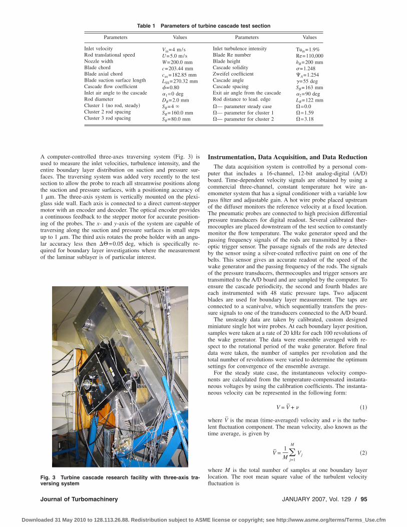
A computer-controlled three-axes traversing system �Fig. 3� isused to measure the inlet velocities, turbulence intensity, and theentire boundary layer distribution on suction and pressure sur-faces. The traversing system was added very recently to the testsection to allow the probe to reach all streamwise positions alongthe suction and pressure surfaces, with a positioning accuracy of1 �m. The three-axis system is vertically mounted on the plexi-glass side wall. Each axis is connected to a direct current-steppermotor with an encoder and decoder. The optical encoder providesa continuous feedback to the stepper motor for accurate position-ing of the probes. The x- and y-axis of the system are capable oftraversing along the suction and pressure surfaces in small stepsup to 1 �m. The third axis rotates the probe holder with an angu-lar accuracy less then ��=0.05 deg, which is specifically re-quired for boundary layer investigations where the measurementof the laminar sublayer is of particular interest.

Instrumentation, Data Acquisition, and Data ReductionThe data acquisition system is controlled by a personal com-

puter that includes a 16-channel, 12-bit analog-digital �A/D�board. Time-dependent velocity signals are obtained by using acommercial three-channel, constant temperature hot wire an-emometer system that has a signal conditioner with a variable lowpass filter and adjustable gain. A hot wire probe placed upstreamof the diffuser monitors the reference velocity at a fixed location.The pneumatic probes are connected to high precision differentialpressure transducers for digital readout. Several calibrated ther-mocouples are placed downstream of the test section to constantlymonitor the flow temperature. The wake generator speed and thepassing frequency signals of the rods are transmitted by a fiber-optic trigger sensor. The passage signals of the rods are detectedby the sensor using a silver-coated reflective paint on one of thebelts. This sensor gives an accurate readout of the speed of thewake generator and the passing frequency of the rods. The signalsof the pressure transducers, thermocouples and trigger sensors aretransmitted to the A/D board and are sampled by the computer. Toensure the cascade periodicity, the second and fourth blades areeach instrumented with 48 static pressure taps. Two adjacentblades are used for boundary layer measurement. The taps areconnected to a scanivalve, which sequentially transfers the pres-sure signals to one of the transducers connected to the A/D board.

The unsteady data are taken by calibrated, custom designedminiature single hot wire probes. At each boundary layer position,samples were taken at a rate of 20 kHz for each 100 revolutions ofthe wake generator. The data were ensemble averaged with re-spect to the rotational period of the wake generator. Before finaldata were taken, the number of samples per revolution and thetotal number of revolutions were varied to determine the optimumsettings for convergence of the ensemble average.

For the steady state case, the instantaneous velocity compo-nents are calculated from the temperature-compensated instanta-neous voltages by using the calibration coefficients. The instanta-neous velocity can be represented in the following form:

V = V + � �1�

where V is the mean �time-averaged� velocity and � is the turbu-lent fluctuation component. The mean velocity, also known as thetime average, is given by

V =1

M �j=1

M

Vj �2�

where M is the total number of samples at one boundary layerlocation. The root mean square value of the turbulent velocityfluctuation is

Table 1 Parameters of turbine cascade test section

Parameters Values Parameters Values

Inlet velocity Vin=4 m/s Inlet turbulence intensity Tuin=1.9%Rod translational speed U=5.0 m/s Blade Re number Re=110,000Nozzle width W=200.0 mm Blade height hB=200 mmBlade chord c=203.44 mm Cascade solidity �=1.248Blade axial chord cax=182.85 mm Zweifel coefficient A=1.254Blade suction surface length LSS=270.32 mm Cascade angle =55 degCascade flow coefficient �=0.80 Cascade spacing SB=163 mmInlet air angle to the cascade �1=0 deg Exit air angle from the cascade �2=90 degRod diameter DR=2.0 mm Rod distance to lead. edge LR=122 mmCluster 1 �no rod, steady� SR=4 � — parameter steady case =0.0Cluster 2 rod spacing SR=160.0 mm — parameter for cluster 1 =1.59Cluster 3 rod spacing SR=80.0 mm — parameter for cluster 2 =3.18

Fig. 3 Turbine cascade research facility with three-axis tra-versing system



� =� 1

M �j=1

M

�Vj − V�2 �3�

and the local turbulence intensity is defined as:

Tuluc =�

V� 100 =

1

V� 1

M �j=1

M

�Vj − V�2 � 100 �4�

For unsteady cases, the ensemble-averaged velocity, fluctuationvelocity, and the turbulence intensity were calculated from theinstantaneous velocity samples by:

Vi�ti� � �Vi�ti� =1

N�j=1

N

Vij�ti� �5�

�i�ti� � ��i�ti� =� 1

N�j=1

N

�Vij�ti� − �Vi�ti��2 �6�

Tui�ti� � �Tui�ti� =��i�ti��Vi�ti�

� 100 �7�

where N=100 is the total number of wake generator periods andM is the number of samples taken per period. �Vi�ti� is theensemble-averaged velocity for the particular boundary layertraverse.

Experimental Results and DiscussionDetailed surface pressure and boundary layer measurements

were performed at Reynolds numbers of 110,000 and 150,000.These Reynolds numbers, which pertain to a typical cruise opera-tion, exhibit a representative value within LPT operating rangebetween 75,000 and 400,000, as discussed by Hourmouziadis�24�. Furthermore, it produces separation bubbles that can be ac-curately measured by miniature hot wire probes. For the Reynoldsnumbers of 110,000 and 150,000, three different reduced frequen-cies were examined. To generate unsteady wakes, cylindrical rodswith the diameter dR=2 mm were chosen to fulfill the similarcriterion that requires the generation of a drag coefficient, CD, thatis approximately equal to the CD of the turbine blade with thechord and spacing given in Table 1 �for details we refer to thestudies in Refs. �23,25��. Furthermore, we define a reduced fre-quency that includes the cascade solidity �, the flow coefficient�, the blade spacing SB, and the rod spacing SR. The reducedfrequency is an extension of Strouhal number, in the sense thatit incorporates the rod spacing SR and the blade spacing SB inaddition to the inlet velocity and wake generator speed. For sur-face pressure measurement, rods with uniform spacing as speci-fied in Table 1 were attached over the entire belt length. Forboundary layer measurement, however, clusters of rods were at-tached, as mentioned previously.

Surface Pressure Distributions. Detailed pneumatic surfacepressure measurements were taken at Re=110,000 and 150,000.For each Reynolds number, three different reduced frequencies,namely =0.0, 1.59, and 3.18, are applied that correspond to therod spacings SR=� �no rod�, 160, and 80 mm. The pressure dis-tributions in Fig. 4 show the results of the steady case and twounsteady cases. The pressure signals inherently signify the time-averaged pressure, because of the internal pneumatic damping ef-fect of the connecting pipes to the transducer. The noticeable de-viation in pressure distribution between the steady and unsteadycases, especially on the suction surface, is due to the drag forcescaused by the moving rods. The drag forces are imposed on themain stream and cause momentum deficiency that leads to a re-duction of the total and static pressure. The time-averaged pres-sure coefficients along the pressure and suction surfaces are plot-ted in Fig. 4. The suction surface �upper portion� exhibits a strong

negative pressure gradient. The flow accelerates at a relativelysteep rate and reaches its maximum surface velocity that corre-sponds to the minimum Cp=−3.5 at s /s0=0.42. Passing throughthe minimum pressure, the fluid particles within the boundarylayer encounter a positive pressure gradient that causes a sharpdeceleration up to s /s0=0.55. This point signifies the beginning ofthe laminar boundary layer separation and the onset of a separa-tion bubble. As seen in the subsequent boundary layer discussion,the separation bubble characterized by a constant Cp plateau ex-tends up to s /s00.74, thus occupying more than 19% of thesuction surface and constituting a large separation. Passing theplateau, the flow first experiences a second sharp decelerationindicative of a process of reattachment, followed by a furtherdeceleration at a moderate rate. On the pressure surface, the flowaccelerates at a very slow rate, reaches a minimum pressure coef-ficient at s /s0=0.42, and continues to accelerate until the trailingedge has been reached. Unlike the suction surface, the pressuresurface boundary layer does not encounter any adverse positivepressure gradient that triggers separation. However, close to theleading edge, a small plateau extending from s /s0=0.08–0.16 in-dicates the existence of a small size separation bubble that mightbe attributed to a minor inlet flow incidence angle.

Fig. 4 Static pressure distributions at two different Re num-bers and reduced frequencies �=0, 1.59, 3.18 „no rod, 160,80 mm…, SS=separation start, SE=separation end



Considering the unsteady case with the reduced frequency =1.59 corresponding to a rod spacing of SR=160 mm, Fig. 4 ex-hibits a slight difference in the pressure distribution between thesteady and unsteady cases. As mentioned above, this deviation isattributed to the momentum deficiency that leads to a reduction ofthe total and static pressure. For Re=110,000, the wakes have areducing impact on the streamwise extent of the separation pla-teau. As seen in Fig. 4�a�, the trailing edge of the plateau hasshifted from s /s0=0.74 to s /s0=0.702. This shift reduced thestreamwise extent of the separation plateau from 19% to 15% ofthe suction surface length which is, in this particular case, 21% ofreduction in streamwise extent of the separation. Increasing thereduced frequency to =3.18 by reducing the rod spacing to SR=80 mm causes a slight shift of the Cp distribution compared with =1.59 case. One should bear in mind that pneumatically mea-sured surface pressure distribution represents a time integral of thepressure events only.

Increasing the Reynolds number to Re=150,000 has notbrought major changes in steady state Cp distribution. However,the combination of higher Reynolds number with unsteady wakesreveals the noticeable deviation on the streamwise extent of theseparation plateau. As seen in Fig. 4�b�, the trailing edge of theplateau has shifted from s /s0=0.74 to s /s0=0.702 for Reynoldsnumber of 150,000. The combination of higher Reynolds numberwith high unsteady wakes introduce fluctuation kinetic energy intothe boundary layer which tends to inhibit the separation tendency.Cp distribution clearly shows that the wake impingement withhigher Reynolds number shortens the streamwise extent of theseparation zone compared to the steady case.

Detailed information regarding the structure of the separationbubble is delivered by means of a detailed unsteady boundarylayer measurement using hot wire probes, as will be discussed inthe subsequent sections.

Time Averaged Velocity and Fluctuation Distributions. Fol-lowing the surface pressure investigations that mainly addressed

the onset and extent of the separation zone discussed previously,comprehensive boundary layer measurements were performed toidentify the streamwise and normal extent, as well as the defor-mation of the separation zone under unsteady wake flow. Thesteady state case serves as the reference configuration.

Consistent with the surface pressure distribution above, the ef-fect of the wake frequency on the time-averaged velocity profilesand fluctuation velocity distribution are presented for one steadyand two unsteady inlet flow conditions on the suction surfacealong 31 streamwise locations for the Reynolds number of110,000, and 41 streamwise locations for the Reynolds number of150,000. After completing the velocity measurements, the bound-ary layer coordinates were transformed into a blade orthogonalcoordinate system. Velocities at blade normal positions were ob-tained by interpolating their transformed values. The resultsshowed almost no difference between the interpolated and nonin-terpolated velocity data. Experimental investigations were per-formed for three different values of =0.0, 1.59, and 3.18. Thesevalues cover the reduced frequency range encountered in LPTdesign and off-design operation conditions.

The effect of wake frequency on time-averaged velocity andvelocity fluctuation distributions is shown in Figs. 5–8 at six rep-resentative streamwise locations for Re=110,000 and Re=150,000. Among 31 streamwise positions measured along thesuction surface, Figs. 5 and 6 display the velocity and fluctuationdistributions at one streamwise position upstream, three positionswithin and two positions downstream of the separation bubble.The diagrams include the steady state data for reference purposes, =0.0 �SR=��, unsteady data for =1.59 �SR=160 mm� and =3.18 �SR=80 mm�.

As Fig. 5 indicates, in the upstream region of the separationbubble the flow is fully attached. At s /s0=0.49, the velocity dis-tributions inside and outside the boundary layer experience ahardly noticeable decrease with increasing the reduced frequency.At the same positions, however, the time-averaged velocity fluc-tuations shown in Fig. 6 exhibit substantial changes within the

Fig. 5 Distribution of time-averaged velocities along the suc-tion surface for steady case �=0 „SR=�… and unsteady cases�=1.59 „SR=160 mm… and �=3.18 „SR=80 mm… at Re=110,000

Fig. 6 Distribution of time-averaged velocity fluctuationsalong the suction surface for steady case �=0 „SR=�… andunsteady cases �=1.59 „SR=160 mm… and �=3.18 „SR=80 mm… at Re=110,000



boundary layer, as well as outside it. The introduction of the pe-riodic unsteady wakes with highly turbulent vortical cores and thesubsequent mixing has systematically increased the free-streamturbulence level from 1.9% in steady case to almost 3% for =3.18 �SR=80 mm�. Comparing the unsteady cases, =1.59 and3.18, with the steady reference case, =0.0, indicates that withincreasing the lateral position of the maximum velocity fluc-tuation shifts away from the wall. This is due to the periodicdisturbance of the stable laminar boundary layer upstream of theseparation bubble.

As Fig. 6 shows, a substantial influence of the wake frequencyis observed inside the separation bubble at s /s0=0.57, s /s0=0.61, and s /s0=0.73. The wake impingement introduces fluctua-tion kinetic energy stemming from its vortical core into theboundary layer, trying to energize it and to reverse the separationtendency. As seen from the velocity profiles, the wake frequencyeffect shortens the bubble height and reduces its streamwise ex-tent. Compared to the steady case, however, the onset of the sepa-ration bubble has not changed substantially. This shows that, al-though the impingement of the vortical wake core periodicallyreduces the separation bubble height, it does not have sufficientmomentum to completely suppress it. Figure 6 displays the detailsof the turbulence fluctuation activities in and outside of the sepa-ration bubble at s /so=0.57, s /so=0.61, and s /so=0.73. Strongturbulent activities are measured within the separation bubble thatextends to the shear layer. Outside the separation bubble, the tur-bulence activities rapidly decrease, approaching the free-streamlevels that correspond to the individual unsteady frequency dis-cussed above. A comparison of the unsteady cases, =1.59 and3.18, with the steady reference case, =0.0, indicates that withincreasing the lateral position of the maximum fluctuation shiftstoward the wall. This is the consequence of the overall decrease ofthe lateral extension of the separation bubble as a result of wakeimpingement.

Close to the bubble trailing edge at s /so=0.73 and s /so=0.77,Fig. 5 shows that the undisturbed flow, =0 �SR=��, still has its

inflectional pattern. The perturbation by impinging the wakescauses the velocity profile to become fully turbulent and attached.Once the profile becomes fully turbulent, increasing the reducedfrequency from =1.59 �SR=160 mm� to =3.18 �SR=80 mm�does not substantially change the velocity distribution pattern.Figure 6 displays the details of the velocity fluctuation activitiesinside and outside of the reattached boundary layer at s /so=0.77and s /so=0.85. As in Fig. 5, once the velocity profile has becomefully turbulent, its corresponding fluctuation distribution remainsalmost unchanged.

In the context of transitional and turbulent boundary layer flowinvestigations, it is worth noting the different behavior of theseboundary layer types. According to the previous investigations bySchobeiri et al. �10–12� in a HP-turbine cascade with transitionalboundary layer throughout, an increased wake frequency causesturbulence fluctuations to rise inside and outside the boundarylayer. However, in the LPT case with the boundary layer separa-tion, once the boundary layer is reattached and the velocity distri-bution assumes a fully turbulent profile, no major changes areobserved either in the velocity or in the fluctuation velocitydistribution.

For Re=150,000, Figs. 7 and 8 display the velocity and veloc-ity fluctuation distributions at the same streamwise locations asdiscussed above. Likewise, the diagrams include the steady state, =0.0, data for reference purposes and the unsteady data for =1.59 and =3.18. Although the results for Re=150,000 showvery similar velocity and fluctuation patterns, it is observed thatthe starting point of the separation bubble and its reattachmentpoint have moved slightly further downstream. This is clearly vis-ible in Fig. 7, at s /so=0.73 and s /so=0.77, where the inflectionalpattern of the velocity profiles indicates that the above streamwisepositions are located close to the trailing edge within the separa-tion bubble. Increasing the frequency from =0 �SR=�� to =3.18 �SR=80 mm� brings the profiles closer to the fully turbulentpattern, without collapsing. The same statement is true for theturbulence fluctuations, Fig. 8, at s /so=0.73 and s /so=0.77. Also,

Fig. 7 Distribution of time-averaged velocity distributionsalong the suction surface for steady case �=0 „SR=�… andunsteady cases �=1.59 „SR=160 mm… and �=3.18 „SR=80 mm… at Re=150,000

Fig. 8 Distribution of time-averaged fluctuation velocitiesalong the suction surface for steady case �=0 „SR=�… andunsteady cases �=1.59 „SR=160 mm… and �=3.18 „SR=80 mm… at Re=150,000



the size of the separation bubble is smaller when compared to thatfor Re=110,000. To achieve a noticeable impact of the Reynoldsnumber on the onset and extent of the bubble, the Reynolds num-ber needed to increase above 150,000.

Temporal Behavior of the Separation Zone Under PeriodicUnsteady Wake Flow. Velocity distributions on the suction sur-face with time as the parameter are plotted in Figs. 9–12 for Re=110,000, 150,000 for rod spacings SR=80 mm and SR=160 mm that correspond to =1.59 and 3.18. The nondimen-sional time �t /�� values are chosen that they represent the tempo-ral states within one full period of wake passing. For Re=110,000, Figs. 9�a�–9�f� show the velocity distributions, insideand outside the boundary layer at fixed s /so locations, experiencemoderate to pronounced changes. Figure 9�a� represents the in-stantaneous velocity distribution upstream of the separation zone,followed by Figs. 9�b�–9�f� which represent the velocity distribu-tions inside the separation zone. In discussing the following re-sults, we simultaneously refer to the wake distribution as well asthe turbulence fluctuation results.

Figure 9�a� exhibits the velocity distribution on the suction sur-face at s /so=0.49. At this streamwise position, the laminar bound-ary layer is subjected to a strong negative pressure gradient. Thevelocity distributions at different �t /�� experience changes inmagnitude that reflect the corresponding changes of the impingingperiodic wake velocity. It is worth noting that, despite the injec-tion of turbulence kinetic energy by the impinging wakes, no localinstantaneous boundary layer transition occurs. This is because ofthe strong negative pressure gradient that prevents the boundarylayer from becoming instantaneously transitional. Instantaneousvelocity distributions inside the separation zone are shown in Figs.9�b�–9�f�.

As a representative case, we discuss the results plotted in Fig.9�e� at s /so=0.65. During the time interval from t /� close to 0.5�1.5, 2.5, etc.� to about t /�=0.75 �1.75, 2.75, etc.�, the separationzone is exposed to the wake external flow with relatively lower

turbulence level. This flow does not have the capability to sup-press the separation zone. Thus, the separation region is clearlyshown by the velocity distributions at t /�=0.5 and t /�=0.75. Asthe wake passes over the blade at s /so=0.65 introducing highturbulence kinetic energy into the boundary layer, the boundarylayer is energized, causing the separation zone to partially reduce.To emphasize this statement, the steady state velocity distributionat the same streamwise position is also plotted in Fig. 9�e� usingfull circles. It shows clearly the separated nature of the boundarylayer which coincides with the instantaneous velocity profile att /�=0.75. Intermediate times reflect the gradual change betweendifferent t /� states as the flow is undergoing the influence of theoncoming wake. Moving to the trailing edge of the separationzone, at s /so=0.73, Fig. 9�f�, a partial reduction in boundary layerthickness as the result of wake impingement is visible, however,the separation zone does not seem to disappear.

Figures 10�a�–10�f� show that the velocity distributions outsidethe boundary layer at fixed s /so locations experience noticeablechanges at =3.18 �SR=80 mm�. Increasing the wake passingfrequency causes the wake turbulence kinetic energy to increase,resulting in a stronger suppression compared with the =1.59�SR=160 mm� case. As seen in Figs. 11 and 12, increasing theReynolds number to 150,000 causes the leading and trailing edgesof the separation bubble to move further downstream. It is alsoobserved that increasing the Reynolds number reduces the size ofthe separation bubble.

The effect of the periodic unsteady wakes on the onset andextent of the separation bubble is shown in Figs. 13–16 for Re=110,000 and 150,000, and for two different frequencies, namely =1.59 and =3.18. These figures display the full extent of theseparation bubble and its behavior under a periodic wake flowimpingement at different t /�. The wake propagation for =1.59and =3.18 is analyzed and the value of t /� corresponds to thepoint in the cycle at which the data acquisition system is triggered.During a rod passing period, the wake flow and the separationbubble undergo a sequence of flow states which are not noticeably

Fig. 9 Distribution of the ensemble-averaged velocity devel-opment along the suction surface for different s /s0 with timet /� as parameter for �=1.59 „SR=160 mm… and Re=110,000




different when the unsteady data are time averaged.Starting with Re=100,000 and =1.59, Fig. 13�a� exhibits the

separation bubble in its full size at t /�=0.25. At this instant oftime, the incoming wakes have not reached the separation bubble.At t /�=0.5, the wake, with its highly turbulent vortical core,passes over the blade and generates high turbulence kinetic en-ergy. At this point, the wake turbulence penetrates into the bubblecausing a strong mass, momentum, and energy exchange betweenthe wake flow and the fluid contained within the bubble. Thisexchange causes a dynamic suppression and a subsequent contrac-tion of the bubble. As the wake travels over the bubble, the size ofthe bubble continues to contract at t /�=0.75 and reaches its mini-mum size at t /�=1.0. At t /�=1, the full effect of the wake on theboundary layer can be seen before another wake appears and thebubble moves back to the original position. Similar results areobserved when operating at the same Reynolds number, Re=110,000, but at a higher reduced frequency, =3.18, Figs.14�a�–14�d�. A comparison of Figs. 14�a�–14�d� with Figs.12�a�–12�d� illustrates the pronounced influence of higher reducedfrequency which causes more frequent penetration of wake turbu-lence into the separation bubble, causing a stronger suppressionand subsequent contraction of the bubble.

Figures 15 and 16 display the behavior of the separation bubbleunder higher Reynolds number, Re=150,000, and reduced fre-quencies, =1.59 and =3.18. While the higher Reynolds num-ber moves the separation bubble further downstream. Similar con-tracting effects as discussed above are observed at =1.59.However, doubling the reduced frequency and increasing the Rey-nolds number is associated with the higher turbulence intensitythat leads to stronger suppression of the separation bubble, asshown in Figs. 15 and 16.

Intermittency AnalysisIntermittency distribution, which identifies whether the flow is

laminar or turbulent inside the boundary layer, is calculated fol-lowing the method of Hedley and Keffer �26�. Instantaneous ve-

locity is sensitized to increase its discriminatory capabilities be-tween turbulent and nonturbulent parts of the signal. For thispurpose, the multiplication of the first derivative of the velocitysignal and the velocity signal is used for further analysis. This iscalled the detector function, S�t�, defined as

S�t� = �u�u

�t� �8�

The above detector function is used by many researchers, includ-ing Antonia and Bradshaw �27�, Kovasznay et al. �28�, Bradshawand Murlis �29�, and Schobeiri and his coworkers �7,12�. A veryrecent paper by Schobeiri �30� extensively discusses different is-sues relative to intermittency based transition modeling. Thoughsensitized detector function separates the turbulent and nonturbu-lent zones of the fluid, there is still some overlap between the twonear the origins. The discrimination between the two zones of theflow will be ideal when the overlap between the two distributionsis minimal or zero. To eliminate the disturbing effects of the ve-locity signal peaks, a smoothing procedure is applied to the S�t�signal. The mean value of ten consecutive S�t� values is calculatedand the ten values are substituted by their mean value of Ssm�t�.After smoothing the detector function, a threshold level C is thenapplied to the smoothed detector function to distinguish betweentrue turbulence and the signal noise. It is defined as

I�t� = �1 when Ssm�t� � C

0 when Ssm�t� � C �9�

Once the threshold level is applied to the detector function S�t�,the result is a random square wave called the indicator function I,with 0’s representing the nonturbulent case and 1’s indicating theturbulent behavior of the boundary layer. A threshold level, C, of1.2 is used for all the data on the suction surface. In the absence oflength scales, this value is chosen from visual observations. Sev-eral other values of C are tested and little qualitative difference isseen in the intermittency distribution during transition. Though the





intermittency values vary with different values of C, the importantparameters like start and end of transition are not affected by C.The resulting square wave after applying the threshold is en-semble averaged to get the ensemble-averaged intermittency asfollows

�i�ti� =1

N�j=1

N

Iij�ti� �10�

where N is the number of revolutions of the wake generator forwhich the data are collected. For time-averaged intermittency,

Fig. 13 Ensemble-averaged velocity contours along the suction surface for different s /s0 withtime t /� as parameter for �=1.59 „SR=160 mm…, Re=110,000




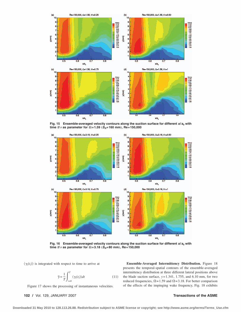
�i�ti� is integrated with respect to time to arrive at

=1

T�t=0

T

�i�ti�dt �11�

Figure 17 shows the processing of instantaneous velocities.

Ensemble-Averaged Intermittency Distribution. Figure 18presents the temporal-spatial contours of the ensemble-averagedintermittency distribution at three different lateral positions abovethe blade suction surface, y=1.341, 1.755, and 6.10 mm, for tworeduced frequencies, =1.59 and =3.18. For better comparisonof the effects of the impinging wake frequency, Fig. 18 exhibits





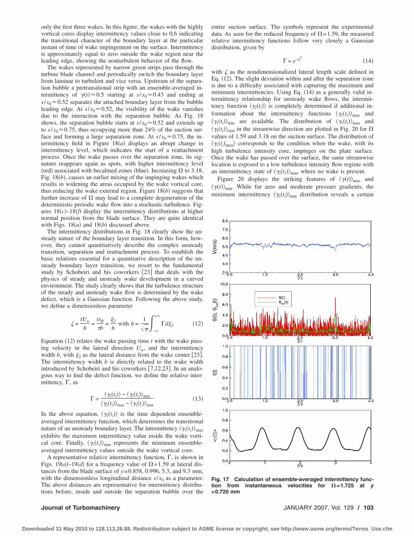
only the first three wakes. In this figure, the wakes with the highlyvortical cores display intermittency values close to 0.6 indicatingthe transitional character of the boundary layer at the particularinstant of time of wake impingement on the surface. Intermittencyis approximately equal to zero outside the wake region near theleading edge, showing the nonturbulent behavior of the flow.

The wakes represented by narrow green strips pass through theturbine blade channel and periodically switch the boundary layerfrom laminar to turbulent and vice versa. Upstream of the separa-tion bubble a pretransitional strip with an ensemble-averaged in-termittency of �t�0.5 starting at s /s00.43 and ending ats /s00.52 separates the attached boundary layer from the bubbleleading edge. At s /s00.52, the visibility of the wake vanishesdue to the interaction with the separation bubble. As Fig. 18shows, the separation bubble starts at s /s00.52 and extends upto s /s00.75, thus occupying more than 24% of the suction sur-face and forming a large separation zone. At s /s00.75, the in-termittency field in Figure 18�a� displays an abrupt change inintermittency level, which indicates the start of a reattachmentprocess. Once the wake passes over the separation zone, its sig-nature reappears again as spots, with higher intermittency level�red� associated with becalmed zones �blue�. Increasing to 3.18,Fig. 18�b�, causes an earlier mixing of the impinging wakes whichresults in widening the areas occupied by the wake vortical core,thus reducing the wake external region. Figure 18�b� suggests thatfurther increase of may lead to a complete degeneration of thedeterministic periodic wake flow into a stochastic turbulence. Fig-ures 18�c�–18�f� display the intermittency distributions at highernormal position from the blade surface. They are quite identicalwith Figs. 18�a� and 18�b� discussed above.

The intermittency distributions in Fig. 18 clearly show the un-steady nature of the boundary layer transition. In this form, how-ever, they cannot quantitatively describe the complex unsteadytransition, separation and reattachment process. To establish thebasic relations essential for a quantitative description of the un-steady boundary layer transition, we resort to the fundamentalstudy by Schobeiri and his coworkers �23� that deals with thephysics of steady and unsteady wake development in a curvedenvironment. The study clearly shows that the turbulence structureof the steady and unsteady wake flow is determined by the wakedefect, which is a Gaussian function. Following the above study,we define a dimensionless parameter

� =tUw

b=

tsR

�b=

�2

bwith b =

1��

−�

+�

�d�2 �12�

Equation �12� relates the wake passing time t with the wake pass-ing velocity in the lateral direction Uw, and the intermittencywidth b, with �2 as the lateral distance from the wake center �23�.The intermittency width b is directly related to the wake widthintroduced by Schobeiri and his coworkers �7,12,23�. In an analo-gous way to find the defect function, we define the relative inter-mittency, �, as

� =�i�ti� − �i�ti�min

�i�ti�max − �i�ti�min�13�

In the above equation, �i�ti� is the time dependent ensemble-averaged intermittency function, which determines the transitionalnature of an unsteady boundary layer. The intermittency �i�ti�max

exhibits the maximum intermittency value inside the wake vorti-cal core. Finally, �i�ti�min represents the minimum ensemble-averaged intermittency values outside the wake vortical core.

A representative relative intermittency function, �, is shown inFigs. 19�a�–19�d� for a frequency value of =1.59 at lateral dis-tances from the blade surface of y=0.858, 0.996, 5.3, and 9.3 mm,with the dimensionless longitudinal distance s /s0 as a parameter.The above distances are representative for intermittency distribu-tions before, inside and outside the separation bubble over the

entire suction surface. The symbols represent the experimentaldata. As seen for the reduced frequency of =1.59, the measuredrelative intermittency functions follow very closely a Gaussiandistribution, given by

� = e−�2�14�

with � as the nondimensionalized lateral length scale defined inEq. �12�. The slight deviation within and after the separation zoneis due to a difficulty associated with capturing the maximum andminimum intermittencies. Using Eq. �14� as a generally valid in-termittency relationship for unsteady wake flows, the intermit-tency function �i�ti� is completely determined if additional in-formation about the intermittency functions �i�ti�max and�i�ti�min are available. The distribution of �i�ti�max and�i�ti�min in the streamwise direction are plotted in Fig. 20 for values of 1.59 and 3.18 on the suction surface. The distribution of�i�ti�max corresponds to the condition when the wake, with itshigh turbulence intensity core, impinges on the plate surface.Once the wake has passed over the surface, the same streamwiselocation is exposed to a low turbulence intensity flow regime withan intermittency state of �i�ti�min, where no wake is present.

Figure 20 displays the striking features of ��t�max and��t�min. While for zero and moderate pressure gradients, theminimum intermittency �i�ti�min distribution reveals a certain

Fig. 17 Calculation of ensemble-averaged intermittency func-tion from instantaneous velocities for �=1.725 at y=0.720 mm



similarity to the one described by the Emmons-Narasimha transi-tion model �31�, the present LPT-flow case with a strong negativepressure gradient associated with separation, �i�ti�min exhibits aremarkably different course that occurs systematically and repro-ducibly for all cases at all y positions over the blade surface.Upstream of the separation bubble, the course of ��t�min with thevalue close to zero indicates a stable nonturbulent character of theboundary layer. A sharp increase in intermittency indicates theseparation begins shortly before the pressure minimum �Fig. 4�has been reached. It is followed by a high intermittency regionthat covers the separation plateau �Fig. 4� and a steep decreasethat is indicative of reattachment. The streamwise location of theintermittency minimum at s /s00.7 coincides with the end of theseparation plateau. The following increase in intermittency is dueto the steep positive pressure gradient that follows the constantpressure plateau. On the other hand, �i�ti�max reveals a funda-

mentally different behavior. As Fig. 20 shows, the wake flow withan intermittency of �i�ti�max0.8–0.9 impinges on the bladesurface. By convecting downstream, because of an extremely thinboundary layer, the wake turbulent fluctuations do not undergo astrong damping by the wall shear stress forces, as was observed inzero and moderate pressure gradient cases reported in Refs.�7,12�.

Utilizing ��t�max and ��t�min, the relative intermittency � isfound to be described by a Gaussian distribution. This observationis in accord with the findings reported in Refs. �7,12�, and veryrecently in Ref. �30� confirming the universal character of �. Con-sidering the intermittency results of the current investigations andthose reported above, it can be concluded that, in general,�i�ti�max and �i�ti�min are not only functions of reduced fre-quency, but they are also strongly influenced by the pressure gra-

Fig. 18 Ensemble-averaged intermittency factor in the temporal-spatial domain at different ypositions for �=1.59 „SR=160 mm… and �=3.18 „SR=80 mm…



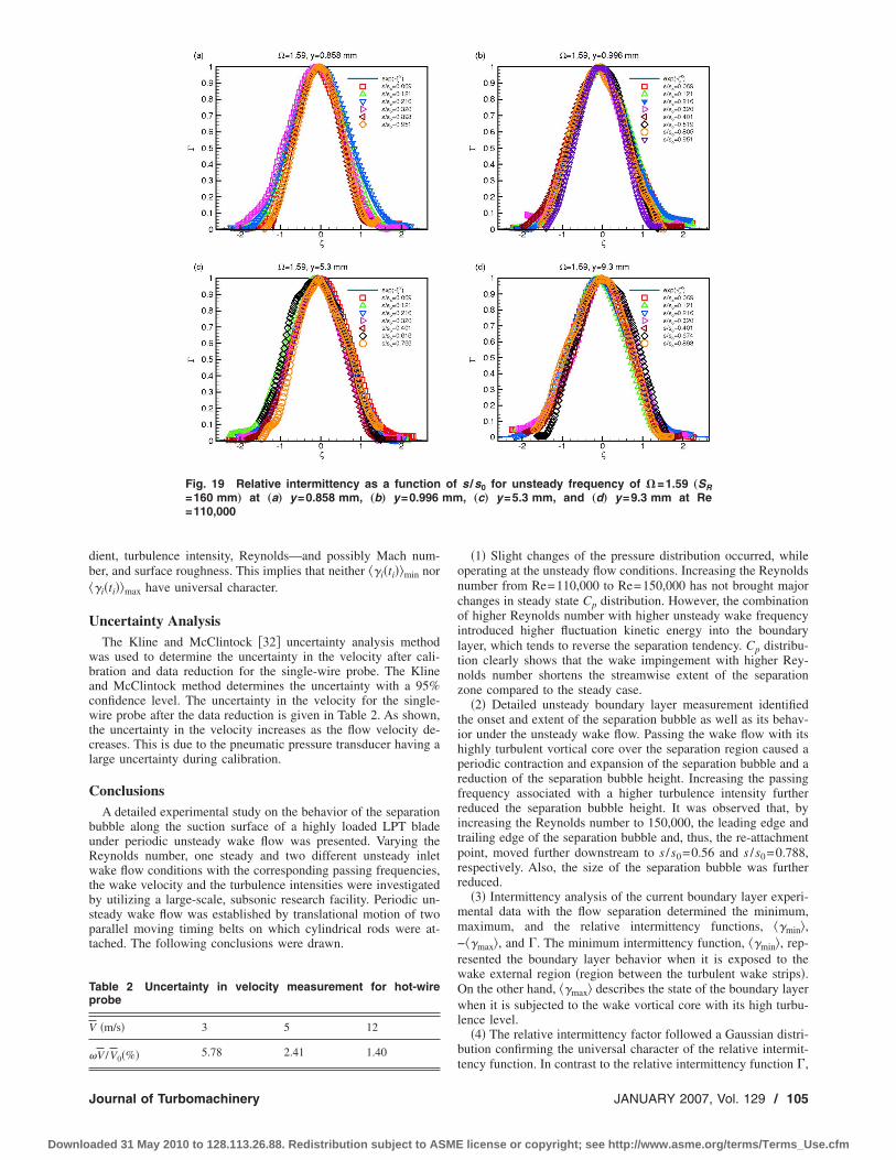
dient, turbulence intensity, Reynolds—and possibly Mach num-ber, and surface roughness. This implies that neither �i�ti�min nor�i�ti�max have universal character.

Uncertainty AnalysisThe Kline and McClintock �32� uncertainty analysis method

was used to determine the uncertainty in the velocity after cali-bration and data reduction for the single-wire probe. The Klineand McClintock method determines the uncertainty with a 95%confidence level. The uncertainty in the velocity for the single-wire probe after the data reduction is given in Table 2. As shown,the uncertainty in the velocity increases as the flow velocity de-creases. This is due to the pneumatic pressure transducer having alarge uncertainty during calibration.

ConclusionsA detailed experimental study on the behavior of the separation

bubble along the suction surface of a highly loaded LPT bladeunder periodic unsteady wake flow was presented. Varying theReynolds number, one steady and two different unsteady inletwake flow conditions with the corresponding passing frequencies,the wake velocity and the turbulence intensities were investigatedby utilizing a large-scale, subsonic research facility. Periodic un-steady wake flow was established by translational motion of twoparallel moving timing belts on which cylindrical rods were at-tached. The following conclusions were drawn.

�1� Slight changes of the pressure distribution occurred, whileoperating at the unsteady flow conditions. Increasing the Reynoldsnumber from Re=110,000 to Re=150,000 has not brought majorchanges in steady state Cp distribution. However, the combinationof higher Reynolds number with higher unsteady wake frequencyintroduced higher fluctuation kinetic energy into the boundarylayer, which tends to reverse the separation tendency. Cp distribu-tion clearly shows that the wake impingement with higher Rey-nolds number shortens the streamwise extent of the separationzone compared to the steady case.

�2� Detailed unsteady boundary layer measurement identifiedthe onset and extent of the separation bubble as well as its behav-ior under the unsteady wake flow. Passing the wake flow with itshighly turbulent vortical core over the separation region caused aperiodic contraction and expansion of the separation bubble and areduction of the separation bubble height. Increasing the passingfrequency associated with a higher turbulence intensity furtherreduced the separation bubble height. It was observed that, byincreasing the Reynolds number to 150,000, the leading edge andtrailing edge of the separation bubble and, thus, the re-attachmentpoint, moved further downstream to s /s0=0.56 and s /s0=0.788,respectively. Also, the size of the separation bubble was furtherreduced.

�3� Intermittency analysis of the current boundary layer experi-mental data with the flow separation determined the minimum,maximum, and the relative intermittency functions, �min,−�max, and �. The minimum intermittency function, �min, rep-resented the boundary layer behavior when it is exposed to thewake external region �region between the turbulent wake strips�.On the other hand, �max describes the state of the boundary layerwhen it is subjected to the wake vortical core with its high turbu-lence level.

�4� The relative intermittency factor followed a Gaussian distri-bution confirming the universal character of the relative intermit-tency function. In contrast to the relative intermittency function �,

Table 2 Uncertainty in velocity measurement for hot-wireprobe

V �m/s� 3 5 12

�V /V0�%� 5.78 2.41 1.40

Fig. 19 Relative intermittency as a function of s /s0 for unsteady frequency of �=1.59 „SR=160 mm… at „a… y=0.858 mm, „b… y=0.996 mm, „c… y=5.3 mm, and „d… y=9.3 mm at Re=110,000



the minimum as well as the maximum intermittency do not sug-gest to have a universal character. Several parameters, such asfree-stream turbulence intensity, reduced frequency, surfaceroughness, Re number, and pressure gradient, are instrumental inaffecting the pattern of these two intermittencies. Future studiesneed to incorporate these parameters.

AcknowledgmentThe study presented is a part of an ongoing LPT-aerodynamics

project executed by the NASA Glenn Research Center. The firsttwo authors were supported by NASA Cooperative AgreementNCC3-793 monitored by Dr. David Ashpis. The support and thepermission for publication are gratefully acknowledged. The au-thors also gratefully acknowledge Pratt & Whitney for providingthe research community with the blade coordinates.

Nomenclatureb � intermittency wake widthc � blade chord

cax � axial chordCp � pressure coefficient, Cp= �pi− ps� / �pt− ps�inlC � threshold level

dR � rod diameterH12 � shape factor, H12=�1 /�2hm � maximum separation bubble height

I�x , t� � indicator functionLSS � suction surface lengthM � number of samplesN � number of wake cyclespi � static pressure taps i=1, . . ,48

ps, pt � static, total pressureReLSS � suction surface Reynolds number

Re=LssVexit /�s � streamwise distance from the leading edge of

the bladesmd � streamwise location of maximum separation

bubble heightso � streamwise distance from the leading edge to

the trailing edge of the bladesr � re-attachment point of the separation bubble

from blade leading edgess � start of the separation bubble at a streamwise

distance from blade leading edgeS�x , t� � criterion function

Fig. 20 Maximum, minimum, and time-averaged intermittency as a function ofs /s0 at different lateral positions for steady case �=0 „SR=�… and unsteady cases�=1.59 „SR=160 mm… and �=3.18 „SR=80 mm… at Re=110,000



SB � blade spacingSR � rod spacing

t � timeTu � reference turbulence intensity

�Tu � ensemble-averaged turbulence intensityU � belt translational velocityv � fluctuation velocityV � velocity

Vax � axial velocityVexit � exit velocity

x � position vectory � lateral distance from plate surface

�1,2 � cascade inlet, exit flow angles � cascade stagger angle � time-averaged intermittency

�� ensemble-averaged intermittency��max � maximum ensemble-averaged intermittency��min � minimum ensemble-averaged intermittency

� � relative turbulence intermittency� � nondimensional coordinate, y /b� � kinematic viscosity

�2 � lateral distance from wake center� � density of air� � cascade solidity, �=c /SB� � one wake-passing period� � flow coefficient, �=Vax/U

�A � Zweifel coefficient�A=2sin2 �2�cot �2−cot �1�SB /cax

� reduced frequency = �c /SR��U /Vax�=�� /��SB /SR�

References�1� Pfeil, H., and Herbst, R., 1979, “Transition Procedure of Instationary Bound-

ary Layers,” ASME Paper No. 79-GT-128.�2� Pfeil, H., Herbst, R., and Schröder, T., 1983, “Investigation of the Laminar

Turbulent Transition of Boundary Layers Disturbed by Wakes,” ASME J. Eng.Power, 105, pp. 130–137.

�3� Orth, U., 1992, “Unsteady Boundary-Layer Transition in Flow PeriodicallyDisturbed by Wakes,” ASME Paper No. 92-GT-283.

�4� Schobeiri, M. T., and Radke, R. E., 1994, “Effects of Periodic Unsteady WakeFlow and Pressure Gradient on Boundary Layer Transition Along the ConcaveSurface of a Curved Plate,” ASME Paper No. 94-GT-327.

�5� Schobeiri, M. T., Read, K., and Lewalle, J., 2003, “Effect of Unsteady WakePassing Frequency on Boundary Layer Transition, Experimental Investigationand Wavelet Analysis,” ASME J. Fluids Eng., 125, pp. 251–266.

�6� Wright, L., and Schobeiri, M. T., 1999, “The Effect of Periodic Unsteady Flowon Boundary Layer and Heat Transfer on a Curved Surface,” ASME J. HeatTransfer, 120, pp. 22–33.

�7� Chakka, P., and Schobeiri, M. T., 1999, “Modeling of Unsteady BoundaryLayer Transition on a Curved Plate under Periodic Unsteady Flow Condition:Aerodynamic and Heat Transfer Investigations,” ASME J. Turbomach., 121,pp. 88–97.

�8� Liu, X., and Rodi, W., 1991, “Experiments on Transitional Boundary Layerswith Wake-Induced Unsteadiness,” J. Fluid Mech., 231, pp. 229–256.

�9� Schobeiri, M. T., Pappu, K., and Wright, L., 1995, “Experimental Study of theUnsteady Boundary Layer Behavior on a Turbine Cascade,” ASME Paper No.95-GT-435.

�10� Schobeiri, M. T., John, J., and Pappu, K., 1997, “Experimental Study on theEffect of Unsteadiness on Boundary Layer Development on a Linear TurbineCascade,” Exp. Fluids, 23, pp. 303–316.

�11� Schobeiri, M. T., and Wright, L., 2003, “Advances in Unsteady Boundarylayer Transition Research: Part I and II,” Int. J. Rotating Mach., 9�1�, pp.1–22.

�12� Schobeiri, M. T., and Chakka, P., 2002, “Prediction of Turbine Blade HeatTransfer and Aerodynamics Using Unsteady Boundary Layer TransitionModel,” Int. J. Heat Mass Transfer, 45, pp. 815–829.

�13� Brunner, S., Fottner, L., and Schiffer, H.-P., 2000, “Comparison of Two HighlyLoaded Turbine Cascade Under the Influence of Wake-Induced Transition,”ASME Paper No. 2000-GT-268.

�14� Cardamone, P., Stadtmüller, P., Fottner, L., and Schiffer, H.-P., 2000, “Numeri-cal Investigation of the Wake-Boundary Layer Interaction on a Highly LoadedLP Turbine Cascade Blade,” ASME Paper No. 2002-GT-30367.

�15� Schulte, V., and Hodson, H. P., 1996, “Unsteady Wake-Induced BoundaryLayer Transition in High Lift LP Turbines,” ASME Paper No. 96-GT-486.

�16� Kaszeta, R., Simon, T. W., and Ashpis, D. E., 2001, “Experimental Investiga-tion of Transition to Turbulence as Affected by Passing Wakes,” ASME PaperNo. 2001-GT-0195.

�17� Lou, W., and Hourmouziadis, J., 2000, “Separation Bubbles Under Steady andPeriodic Unsteady Main Flow Conditions,” ASME Paper No. 200-GT-270.

�18� Schröder, Th., 1989, “Measurements With Hot-Film Probes and SurfaceMounted Hot Film Gages in a Multi-Stage Low Pressure Turbine,” EuropeanPropulsion Forum, Bath, UK.

�19� Haueisen, V., Hennecke, D. K., and Schröder, T., 1997, “Measurements WithSurface Mounted Hot Film Sensors on Boundary Layer Transition in WakeDisturbed Flow,” AGARD-CP-598.

�20� Halstead, D. E., Wisler, D. C., Okiishi, T. H., Walker, G. J., Hodson, H. P., andShin, H.-W., 1997, “Boundary Layer Development in Axial Compressors andTurbines: Part 3 of 4,” ASME J. Turbomach., 119, pp. 225–237.

�21� Schobeiri, M. T., and Öztürk, B., 2003, “On the Physics of the Flow Separa-tion Along a Low Pressure Turbine Blade Under Unsteady Flow Conditions,”ASME Paper No. 2003-GT-38917, ASME J. Fluids Eng., 127, pp. 503–513.

�22� Schobeiri, M. T., and Öztürk, B., 2004, “Experimental Study of the Effect ofthe Periodic Unsteady Wake Flow on Boundary Layer Development, Separa-tion, and Re-Attachment Along the Surface of a Low Pressure Turbine Blade,”ASME J. Turbomach., 126�4�, pp. 663–676.

�23� Schobeiri, M. T., John, J., and Pappu, K., 1996, “Development of Two-Dimensional Wakes Within Curved Channels, Theoretical Framework and Ex-perimental Investigation,” ASME J. Turbomach., 118, pp. 506–518.

�24� Hourmouziadis, J., 1989, “Blading Design for Axial Turbomachines,”AGARD, Lecture Series LS-167.

�25� Eifler, J., 1975, “Zur Frage der freien turbulenten Strömungen, insbesonderehinter Ruhenden und bewegten Zylindern,” Dissertation D-17, TechnischeHochschule Darmstadt, Germany.

�26� Hedley, B. T., and Keffer, F. J., 1974, “Turbulent/Non-Turbulent Decisions inan Intermittent Flow,” J. Fluid Mech., 64, pp. 625–644.

�27� Antonia, R. A., and Bradshaw, P., 1971, Imp. College Aero. Rep. No. 71–04.�28� Kovasznay, L. S. G., Kibens, V., and Blackwelder, R. F., 1970, J. Fluid Mech.,

41, p. 283.�29� Bradshaw, P., and Murlis, J., 1973, Imp. College Aero. Tech. Note, No. 73–

108.�30� Schobeiri, M. T., 2005, “Intermittency Based Unsteady Boundary Layer Tran-

sition Modeling, Implementation Into Navier-Stokes Equations,” ASME PaperNo. GT2005–68375.

�31� Dhawan, S., and Narasimha, R., 1958, “Some Properties of Boundary LayerFlow During The Transition From Laminar to Turbulent Motion,” J. FluidMech., 3, pp. 418–436.

�32� Kline, S. J., and McKlintock, F. A., 1953, “Describing Uncertainties in Single-Sample Experiments,” Mech. Eng. �Am. Soc. Mech. Eng.�, 75, pp. 3–8.



M. P. C. van Rooij1

T. Q. Dang

Syracuse University,Syracuse, NY 13244

L. M. Larosiliere2

U.S. Army Research Laboratory,NASA Glenn Research Center,

Cleveland, OH 44135

Improving Aerodynamic Matchingof Axial Compressor BladingUsing a Three-DimensionalMultistage Inverse DesignMethodCurrent turbomachinery design systems increasingly rely on multistage CFD as a meansto diagnose designs and assess performance potential. However, design weaknesses at-tributed to improper stage matching are addressed using often ineffective strategies in-volving a costly iterative loop between blading modification, revision of design intent,and further evaluation of aerodynamic performance. A scheme is proposed herein whichgreatly simplifies the design point blade row matching process. It is based on a three-dimensional viscous inverse method that has been extended to allow blading analysis anddesign in a multi-blade row environment. For computational expediency, blade row cou-pling is achieved through an averaging-plane approximation. To limit computationaltime, the inverse method was parallelized. The proposed method allows improvement ofdesign point blade row matching by direct regulation of the circulation capacity of theblading within a multistage environment. During the design calculation, blade shapes areadjusted to account for inflow and outflow conditions while producing a prescribedpressure loading. Thus, it is computationally ensured that the intended pressure-loadingdistribution is consistent with the derived blading geometry operating in a multibladerow environment that accounts for certain blade row interactions. The viability of themethod is demonstrated in design exercises involving the rotors of a 2.5 stage, highlyloaded compressor. Individually redesigned rotors display mismatching when run in the2.5 stage, evident as a deviation from design intent. However, simultaneous redesign ofthe rotors in their multistage environment produces the design intent, indicating thataerodynamic matching has been achieved. �DOI: 10.1115/1.2372773�

Keywords: inverse aerodynamic shape design, multistage turbomachinery CFD, com-pressor stage matching

IntroductionTurbomachinery computational fluid dynamics �CFD�, in sup-

port of aerodynamic design, has evolved from isolated blade rowmethods to hierarchical multistage analysis encompassing variousblade row coupling schemes. Three main approaches to blade rowcoupling exist: steady averaging plane, time mean average pas-sage, and unsteady time periodic. The foundations of these ap-proaches are discussed in Refs. �1,2�. Currently, multistage CFDmethods are primarily suited for diagnosing design shortcomingsoriginating from strong blade row interactions that adversely im-pact performance and operability. Typically, simulation results areused to revise aerodynamic matching conditions for individualblade rows and stages. The term aerodynamic matching is looselyunderstood to involve the compatibility of the inlet flow require-ments of a stage to the outlet flow of upstream stages.

In the title of this paper, the word “matching” denotes a criticalfunction of the multi-blade row design process, where the indi-vidual blade row shapes are simultaneously tailored in such a wayas to produce a desired design intent while accounting for blade

row interactions that would lead to deviations from this designintent. The “design intent” implies a physically realizableaxisymmetric-averaged pressure field that is compatible withoverall design point performance and off-design operability. For agiven overall pressure rise, mismatching is manifested as a dis-ruption of the design equilibrium among the circulation capacityof the blading, entropy production, and accumulation of aerody-namic blockage. Naturally, an appropriate choice of design intentcan limit strong blade row interactions.

There are two key elements in the blade row matching problem.First, there is the establishment of accurate and physically realiz-able design intent and, second, when necessary, an efficient meansfor tailoring blade shapes so that design equilibrium is restoredamong blading circulation capacity, entropy production, and accu-mulation of aerodynamic blockage. Transforming overall func-tional requirements into credible aerodynamic design intent is aninherently iterative process guided by past experience. Note thatthis is compatible with the traditional model for turbomachineryaerodynamic design, as described by Marble �3�, whereby theflow is conceptually decomposed into two parts: that which is dueto the gross influence of all blade rows and that which is associ-ated with local details of blade shape.

A contemporary aerodynamic design system, incorporatingmultistage CFD analysis, is noted in Fig. 1�a�. This system allowstwo broad functions: design synthesis, and design diagnostics anddevelopment. Both of these functions can be iteratively executedto arrive at credible design intent and a blading revision strategy

1Present address: Siemens Power Generation Industrial Applications.2Present address: Concepts NREC.Contributed by the International Gas Turbine Institute �IGTI� of ASME for pub-

lication in the JOURNAL OF TURBOMACHINERY. Manuscript received October 1, 2004;final manuscript received February 1, 2005. IGTI Review Chair K. C. Hall. Paperpresented at the ASME Turbo Expo 2005: Land, Sea and Air, Reno, NV, June 6–9,2005, Paper No. GT2005-68271.



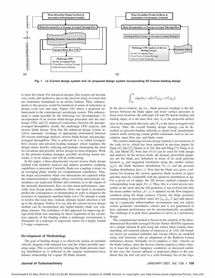
to meet this intent. For advanced designs, this system can becomevery costly and ineffective due to the need for many revisions thatare sometimes formulated in an ad-hoc fashion. Thus, enhance-ments to this process would be beneficial in terms of reductions indesign cycle cost and time. Figure 1�b� shows a proposed en-hancement to the contemporary aerodesign system. This enhance-ment is made possible by the following two developments: �1�incorporation of an inverse blade-design procedure into the mul-tistage CFD, and �2� improved consistency between the passage-averaged throughflow model, the multistage CFD analysis, andinverse blade design. Note that the enhanced design system in-volves automatic exchange of appropriate information between3D viscous multistage analysis, inverse blade design, and passage-averaged throughflow. This is achieved by a so called averaged-flow closure and pressure-loading manager which regulates thedesign intent, thereby reducing and perhaps eliminating the needfor circuitous and possibly ad-hoc design revision strategies. Workon the pressure-loading manager, possibly involving neural net-works, is in its infancy and will be forthcoming.

In this paper, a three-dimensional viscous inverse blade designmethod with multirow analysis and indirect geometric sculptingcapabilities is presented. Currently, blade row coupling is done viaan averaging plane, mainly for computational expediency. Thus,the major axisymmetric blade row interactions are captured whilethe nonaxisymmetric coupling effects involving deterministic un-steadiness are neglected. Debate still continues as to the impact ofthe unsteady deterministic flow on time-mean performance, espe-cially near design point conditions. Does one need to accuratelypredict the consequences of mismatching in order to diagnose theexistence of improperly matched blade rows? No attempt is madeto resolve this issue here; instead, ultimate model selection is leftup to the designer. Suffice it to say that the current inverse designmethod can be incorporated into higher-fidelity blade row cou-pling schemes. The usefulness of this approach for improving de-sign point blade row matching by direct regulation of the circula-tion capacity of the blading within a multistage environment isillustrated via a redesign of supersonic rotors for a highly loaded2.5-stage compressor.

Development of MethodologyThe goal of blading design is to effectively realize an intended

velocity diagram with minimal loss and the widest possible oper-ating range. This is achieved by tailoring the blade pressure load-ing distribution as is reflected in the angular momentum-forcebalance relationship for a quasi-3D blade element

�LE

TE

r�pdA� � m��rV��TE − �rV��LE�

In the above relation, �p �i.e., blade pressure loading� is the dif-ference between the blade upper and lower surface pressures atfixed axial locations; the subscripts LE and TE denote leading andtrailing edges; m is the mass flow rate; A� is the projected surface

area in the tangential direction; and rV� is the mass-averaged swirlvelocity. Thus, the overall blading design strategy can be de-scribed as pressure-loading tailoring to attain local aerodynamiccontrol while satisfying certain global constraints such as net cir-culation, mass flow rate, and blade count.

The current multistage inverse design method is an extension ofthe code INV3D, which has been reported in previous papers byDang �4�, Qiu �5�, Damle et al. �6�, Qiu and Dang �7�, Dang et al.�8�, and Medd �9�. Note that INV3D can be used for both designand analysis. In the inverse mode, the primary prescribed quanti-ties are the blade axis definition in terms of its axial grid-linelocation iba and tangential orientation along the camber surfacefba�r�, the blade thickness distribution T�r ,z�, and the pressureloading distribution �p�r ,z�. Note that the blade axis gives a ref-erence for locating the various spanwise blade sections in spaceand thus must be compatible with the spanwise distribution of �p.For a given set of inputs, the 3D inverse method computes thecorresponding wrap angle f�r ,z�. Thus, this is a semi-inverse pro-cedure in the sense that the full geometry is not evolved and onlythe mean camber surface, f�r ,z�, is updated via the flow-tangencycondition along the blade surfaces. Clearly, the blade geometrycorresponding to prescribed values for �iba , fba ,T ,�p� and operat-ing in a particular inflow/outflow environment may not satisfycertain geometric smoothness criteria and is not guaranteed tohave optimum performance nor be aeromechanically acceptable.The challenge is to pick these quantities to arrive at a satisfactorydesign.

The computational method is based on the solution of the three-dimensional Reynolds-averaged Navier–Stokes �RANS� equationson a simple sheared H grid using the robust finite-volume time-marching cell-centered scheme of Jameson et al. �10�. All bound-ary layers are assumed turbulent and viscous effects are modeledusing wall functions with an adaptation of the Baldwin–Lomaxturbulence closure. Normally, INV3D employs a “slip” velocity onthe blade surface, since the inverse scheme requires a finite veloc-ity to trace the surface �tangency condition�, as discussed earlier.In this case, the viscous sublayer is neglected subject to the con-dition that the first cell next to a solid boundary lies in the loga-

Fig. 1 „a… Current design system and „b… proposed design system incorporating 3D inverse blading design



rithmic region and hence the existence of a slip velocity �11�.Typical viscous calculations using INV3D employ near-wall y+ onthe order of 30–150. Leakage flows are approximated by assum-ing periodicity across the extended blade surfaces in the clearancegap.

In order to transform the original research code into a practicaltool, several modifications were made to the basic methodologydescribed by Dang �4� and Dang et al. �8�. The two most criticalmodifications are: �1� the solution method for the camber surfacegenerator, and �2� a hybrid inverse/analysis scheme to handle theblade leading and trailing edges.

In the original method, the camber surface is developed byenforcing the condition of zero-normal velocity on the blade sur-face. The resulting equation for the camber wrap angle f�r ,z� is aconvective equation, the so-called camber generator equation. It isbasically a stream surface tracer, the stream surface being theblade surface. In the original method, the camber generator equa-tion is solved using the implicit Crank–Nicholson scheme. Thisapproach was demonstrated to work very well for inviscid flows�8�, but it is not robust for practical problems involving significantviscous effects and leakage flows. In the latter case, the streamlinein the clearance region is highly three dimensional, resulting inthe blade shape being exceedingly distorted during the iterativeprocess.

Rather than solving the camber generator “exactly” with a con-ventional implicit numerical method as in the original methodol-ogy described in Dang et al. �8�, the camber generator equation issatisfied by minimization in the least squares sense, with the span-wise variation of the camber defined in terms of a NURBS curve�9�. In essence, the camber is generated by fitting the blade as bestas possible to the velocity field. This is done in the spanwisedirection at each axial location of the grid, followed by a geo-metrical smoothing in the chordwise direction. The originallyspecified blade axis is maintained. This method is very robust, andmakes it possible to obtain smooth blade geometries and goodconvergence in the presence of strong clearance leakage flow.

As this is a minimization process, it cannot be guaranteed thatthe local normal velocity be driven to zero during convergence ofthe design calculation. This again implies that the specified load-ing distribution may not be strictly enforced. However, this isoutweighed by the advantages of increased robustness and geo-metrically smoother blade shapes. To obtain a satisfactory balancebetween smoothness and accuracy, the number of NURBS controlpoints used in the spanwise and chordwise directions can be var-ied. The more points used, the closer the normal velocity is drivento zero and the more strictly the specified loading is enforced, butat a cost of smoothness and possibly convergence �e.g., in thepresence of strong leakage flow�.

Another important modification to the original method is theimplementation of a hybrid inverse/analysis technique to handlethe blade leading and trailing edges. Experience with applicationof the inverse method to the design of highly loaded transonicblades, revealed the need for the inverse method to preserve theblade leading-edge detailed geometry in order to capture impor-tant local flow structures. For example, the grid must be clusterednear the leading edge so that the incoming flow sees the bladeleading edge as blunt rather than sharp. However, highly clusteredsheared H grids near the leading edge can result in convergencedifficulties initiated by possible distortion of the blade leadingedge shape. This is due to the fact that near the leading edge, gridskewness, and dispersion errors can create a locally distorted ve-locity field, and since the blade shape is traced from this velocityfield, it too will be distorted. Thus, in order to maintain geometri-cally accurate leading and trailing edge shapes during the designprocess, a hybrid inverse technique is used �9�. Here, the leadingand trailing edge geometries are created by extrapolation of theblade camber surface from the interior using a NURBS curve. Themeridional envelope of the blade is maintained. Analysis bound-ary conditions are specified in these regions, which typically en-compass 1–5% of the blade chord. Apart from geometric fidelity,this method also increases robustness of the camber generator inthe presence of exceedingly high swirl angles that are typical ofmultistage end wall flows at the design point. It may not be de-sirable to sustain high local gradients in the blade edge angles, andthe 3D relief phenomenon discussed in Wadia and Beacher �12�tends to accommodate smooth blades.

The INV3D solver is able to predict the static pressure field withreasonable accuracy along with adequate resolution of most criti-cal flow structures responsible for relative changes in the entropyproduction mechanisms �e.g., when massive flow separation is notpresent�. Figure 2 shows overall total pressure ratio characteristicsand axisymmetric-averaged spanwise profiles of adiabatic effi-ciency for NASA rotor 37 �13� comparing results from INV3D bothwith and without wall slip against measurements �14�. Also indi-cated, are results using the NASA developed multiblock RANScode, ADPAC �15�. Both INV3D and ADPAC show good agreementwith the spanwise distribution of efficiency inferred from mea-surements. The absolute level of total pressure is not well pre-dicted and could be improved with better viscous and/or turbu-lence modeling. Overall, the agreement with measurements isadequate in the sense that INV3D does identify critical flow struc-tures responsible for relative changes in performance.

INV3D was extended to multistage by adding a blade row cou-pling scheme and parallelization. Currently, blade row couplingfor multistage calculations is achieved by a steady averaging-plane approximation. Two versions have been implemented. The

Fig. 2 Comparison between measured data and CFD simulations of NASA rotor 37 using INV3D

and ADPAC: „a… performance map of total pressure ratio versus mass flow and „b… exit spanwiseprofile of total-to-total adiabatic efficiency at nominal operation



first involves direct exchange of circumferentially averaged den-sity, momentum and pressure across the averaging-plane �11,16�.The second, considered to be numerically superior, is an adapta-tion of the nonreflecting averaging plane presented by Chima �17�,which is based on characteristic boundary conditions derived byGiles �18�. It is recognized that the steady averaging-plane cou-pling ignores much, if not all, of the physics associated with de-terministic unsteadiness inherent to multistage turbomachineryflows. However, it does provide spanwise consistency in the con-servative variables along with global mass conservation therebyallowing first-order axisymmetric blade row interactions to becaptured. Due to ease of implementation and computational con-venience, as a first step, the averaging-plane blade row couplingwas therefore chosen for exploring the potential of blade inversedesign in a multistage environment.

Because of the extensive computational demand of a multistagecalculation, the ability to exploit parallel processing computingcapability has been added to the code in the form of MPICH

�19,20�. For a parallel run, each blade row is assigned to a slaveprocess on a separate processor, while a master process handles allthe input and output. A cluster of 5 AMD XP2400� PCs runningWindows 2000 has been used for all calculations presented here.

Aerodynamic Matching StudyA meridional cross section of the 2.5-stage advanced compres-

sor used to illustrate the viability of blade inverse design for im-proving blade row matching in a multistage environment is shownin Fig. 3. The design philosophy of this compressor is given inLarosiliere et al. �21�; however, the current blading set is a variantof that described in the reference. Design features include variableinlet guide vane, cantilevered stators, and 3D blading. The com-pressor can be characterized as generally high Mach number, highreaction, and highly loaded. Rotor 2 has supersonic relative inletMach numbers along its entire span, thus exacerbating the stage-matching problem. The aerodynamic design requirements for thiscompressor are a corrected mass flow of 31.8 kg/s �70 lbm/s�, anoverall total compression ratio of 4.65:1 �at shroud backpressureof 4.0�, a total pressure ratio of 2.42:1 across rotor 1 with a cor-rected tip speed of 450.2 m/s �1477 ft/ s�, and a rotor 2 totalpressure ratio of 2.0:1 at a corrected tip speed of 393.2 m/s�1290 ft/ s�.

This compressor was originally designed using a contemporarydesign system similar to that noted in Fig. 1�a�. An earlier isolatedblade row version of INV3D �i.e., rudimentary viscous model, lowmesh resolution, and basic inverse scheme�, with aerodynamicmatching conditions extracted from a design point throughflowmodel, was used to refine the rotor blade shapes in an attempt tobetter manage the passage shock structure and strength �see Ref.�21� for details�. Note that the credibility of the design-intentaxisymmetric-averaged pressure field from the design point

throughflow model is debatable and indicates the need for estab-lishing consistency among the various mathematical formulationsand physical model closures. Overall, the blading design objectivewas to achieve efficient design point operation at very high aero-dynamic loading levels �i.e., average Lieblein D-factors �0.55�.

The computational mesh used in the present study consisted of51 cells in the axial direction along the blade surface �for eachblade row�, 45 cells in the radial direction, and 35 cells in thepitchwise direction. Three cells were placed in the rotor tip andstator hub gaps �clearances ranging from 0.5% to 1% local chord�.In the analysis mode, this mesh size requires approximately 1 hfor 1500 time steps using 5 AMD XP2400� processors �one pro-cessor for each blade row�. A single blade row calculation takesabout 2000 iterations to convergence. A multistage calculationtypically requires more iterations, since errors propagate throughmultiple blade rows and the blade row coupling itself affects over-all convergence. For the 2.5-stage geometry presented here, about6000 iterations were needed to reach convergence, correspondingto a computational time of 4 h. Compared to the analysis mode,the inverse mode takes about 10% longer per iteration. For allcases presented, the same profiles of total pressure, total tempera-ture, and radial and absolute tangential flow angles were pre-scribed at the inlet of the computational domain. A design pointbackpressure of 4.00 �normalized to inlet total pressure at mid-span� was specified at the casing, and simple radial equilibriumwas used to construct the spanwise exit static pressure profile. Thestandard averaging-plane approach �11,16� was used for steadyblade row coupling.

Diagnosis of Original Blading Geometry. The complete 2.5stage with the original blading geometry was analyzed at thedesign-intent backpressure and speed using INV3D in the analysismode. Diagnostic plots of results for the original geometry areshown in Figs. 4–6, which are described in the following. Figure4 shows contours of relative Mach number at 3%, 50%, and 100%span. Three important conclusions can be made by inspection: �1�generation of significant aero blockage by strong leakage/shockinteraction near the casing end wall of both rotors, �2� existence ofa strong quasi-normal passage shock at the mouth of rotor 2 ex-tending from hub to near midspan, and �3� evolution of separatedsuction-side corner flow near rotor 2 hub inducing increased aeroblockage production in the downstream stator �S2� hub clearanceregion. Thus, based on INV3D analysis at the design-intent back-pressure, the original blading set is forced into an off-design op-eration due to aerodynamic mismatching.

Further insight into the nature of the design point mismatchingcan be gleaned from the predicted pressure-loading distributionsfor R1 �Fig. 5� and R2 �Fig. 6�. These figures show three plotseach. The first plot indicates the pressure-loading distribution,�p�r ,z�, for the original blading resulting from a multistageanalysis at the design backpressure; the second plot is for an iso-lated analysis of each rotor using inflow/outflow conditions fromthe design point throughflow model; and the third plot is thedesign-intent pressure-loading distribution to be discussed shortly.A comparison of the multistage and isolated analysis results givenin Fig. 5 indicates that R1 does not experience significant multi-stage design point mismatching effects; rather there exists a strongtip leakage/shock interaction resulting in larger aero blockage thanintended. A similar comparison for R2, shown in Fig. 6, indicatessignificant multistage design point mismatch. The hub cornerseparation appears to be eliminated or greatly reduced for theisolated analysis of R2, which can be discerned by a comparisonof the two loading distributions �i.e., Fig. 6�a� versus Fig. 6�b�with low �p implying separation� along the hub section. It isevident that the passage shock for R2 is close to being spilled.Indeed, throttling the 2.5 stage to a higher backpressure of 4.02leads to the passage shock of R2 being spilled completely, shortlyfollowed by a numerical stall of the 2.5 stage.

To explore the viability of the inverse method for facilitating

Fig. 3 Meridional flow path for the 2.5-stage compressor usedin the design examples: Inlet guide vane „IGV…, rotor 1 „R1…,stator 1„S1…, rotor 2 „R2… and stator 2 „S2…; rotor 1: 26 blades,average solidity�2.16, aspect ratio�0.83; rotor 2: 56 blades,average solidity�1.96, aspect ratio�0.86. Also indicated, aremultistage computational averaging planes.



and improving design point matching, two design exercises havebeen executed. In the first, R1 and R2 are redesigned in isolationusing the latest improved version of INV3D. Inflow and outflowconditions are specified in accordance with a design point

throughflow model of the original design. The second involves theredesign of both rotors simultaneously within the multistage en-vironment. Both cases employ exactly the same pressure-loadingdistributions. Design-intent pressure-loading distributions for the

Fig. 4 Diagnosis „multistage analysis… of flow structure induced by original geometry at de-sign point in terms of contours of relative Mach number at 3%, 50%, and 100% „rotor blade tip…span. IGV and exit region are not shown for clarity.



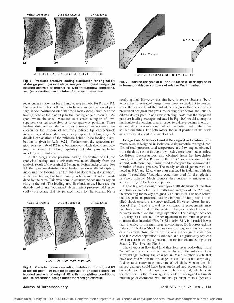
redesigns are shown in Figs. 5 and 6, respectively, for R1 and R2.The objective is for both rotors to have a single swallowed pas-sage shock, positioned such that the shock extends from near thetrailing edge at the blade tip to the leading edge at around 25%span, where the shock weakens as it enters a region of low-supersonic or subsonic flow at lower spanwise positions. Theseloading distributions, derived from numerical experiments, arechosen for the purpose of achieving reduced tip leakage/shockinteraction, and to enable larger design-speed throttling range. Adetailed explanation of the rationale behind these loading distri-butions is given in Refs. �9,22�. Furthermore, the separation re-gion near the hub of R2 is to be removed, which should not onlyimprove overall throttling capability but also provide bettermatching with Stator 2.

For the design-intent pressure-loading distribution of R1, thespanwise loading area distribution was taken directly from theanalysis result of the original 2.5 stage at design backpressure. ForR2, the spanwise distribution of loading area was altered slightly,increasing the loading near the hub and decreasing it elsewhere,while maintaining the total loading volume and therefore workdone by the rotor. This was done to counter the separation regionclose to the hub. The loading area distributions used here are notdirectly tied to any “optimized” design-intent pressure field, espe-cially considering that the passage shock for the original R2 is

nearly spilled. However, the aim here is not to obtain a “best”axisymmetric-averaged design-intent pressure field, but to demon-strate the feasibility of the multistage design method to enforce aprescribed design-intent pressure-loading distribution and thus fa-cilitate design point blade row matching. Note that the proposedpressure-loading manager indicated in Fig. 1�b� would attempt tomanipulate the loading area in order to achieve design-intent av-eraged static pressure distributions consistent with other pre-scribed quantities. For both rotors, the axial position of the bladeaxis was set at about 20% axial chord.

Design Case A: Rotors 1 and 2 Redesigned in Isolation. Bothrotors were redesigned in isolation. Axisymmetric-averaged pro-files of total pressure, total temperature and flow angles, obtainedfrom the design point throughflow model, were specified as inflowconditions. Backpressures, also obtained from the throughflowmodel, of 1.645 for R1 and 3.48 for R2 were specified at theshroud, with radial equilibrium used to compute the spanwise dis-tribution of static pressure. The newly obtained geometries, de-noted as R1A and R2A, were then analyzed in isolation, with thesame “throughflow” boundary conditions used for the redesign.Predicted relative Mach number distributions at midspan areshown in Fig. 7 for later comparison.

Figure 8 gives a design point �pb=4.00� diagnosis of the flowstructure as predicted by a multistage analysis of the 2.5 stageincorporating the newly designed R1A and R2A. For both rotors,the design-intent pressure-loading distribution along with its im-plied shock structure is nearly realized. However, closer inspec-tion of Figs. 7 and 8 reveal the existence of aerodynamic mis-matching manifested by the relative changes in shock structurebetween isolated and multistage operations. The passage shock forR2A �Fig. 8� is situated further upstream in the multistage envi-ronment than intended �Fig. 7�. Similarly, R1A is throttled lowerthan intended in the multistage environment. Both rotors exhibitreduced tip leakage/shock interaction resulting in a much cleanercasing endwall flow than that of the original design. The suction-side hub corner separation is subdued and a significantly reducedlevel of aero blockage is generated in the hub clearance region ofStator 2 �Fig. 4 versus Fig. 8�.

The changes in flow field �and therefore pressure-loading� from“intent” imply some sort of mismatching of the rotors to theirsurroundings. Noting the changes in Mach number levels thathave occurred within the 2.5 stage, this in itself is not surprising.It does raise many questions, one of which is whether the ob-served changes could have been predicted and accounted for inthe redesign. A simpler question to be answered, which is at-tempted here, is the following: if a blade is redesigned within itsmultistage environment, will the design adapt to this �possibly

Fig. 5 Predicted pressure-loading distribution for original R1at design point: „a… multistage analysis of original design, „b…isolated analysis of original R1 with throughflow conditions,and „c… prescribed design intent for redesign exercise

Fig. 6 Predicted pressure-loading distribution for original R2at design point: „a… multistage analysis of original design, „b…isolated analysis of original R2 with throughflow conditions,and „c… prescribed design intent for redesign exercise

Fig. 7 Isolated analysis of R1 and R2 „case A… at design pointin terms of midspan contours of relative Mach number



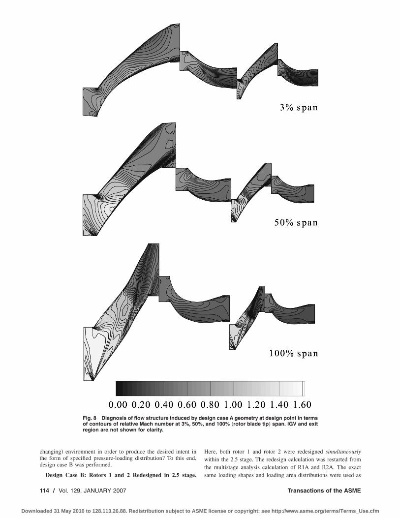
changing� environment in order to produce the desired intent inthe form of specified pressure-loading distribution? To this end,design case B was performed.

Design Case B: Rotors 1 and 2 Redesigned in 2.5 stage.

Here, both rotor 1 and rotor 2 were redesigned simultaneouslywithin the 2.5 stage. The redesign calculation was restarted fromthe multistage analysis calculation of R1A and R2A. The exactsame loading shapes and loading area distributions were used as

Fig. 8 Diagnosis of flow structure induced by design case A geometry at design point in termsof contours of relative Mach number at 3%, 50%, and 100% „rotor blade tip… span. IGV and exitregion are not shown for clarity.



in design case A. The convergence rate in camber during the de-sign calculation was lower than in the isolated designs. This wasexpected, because the blades have to adapt to changing inlet andexit conditions during the design calculation. However, the same

level of convergence was ultimately reached as in the isolateddesigns. The rotor geometries obtained here are denoted as R1Band R2B.

Results of the subsequent design point multistage analysis with

Fig. 9 Diagnosis of flow structure induced by design case B geometry at design point in termsof contours of relative Mach number at 3%, 50%, and 100% „rotor blade tip… span. IGV and exitregion are not shown for clarity.



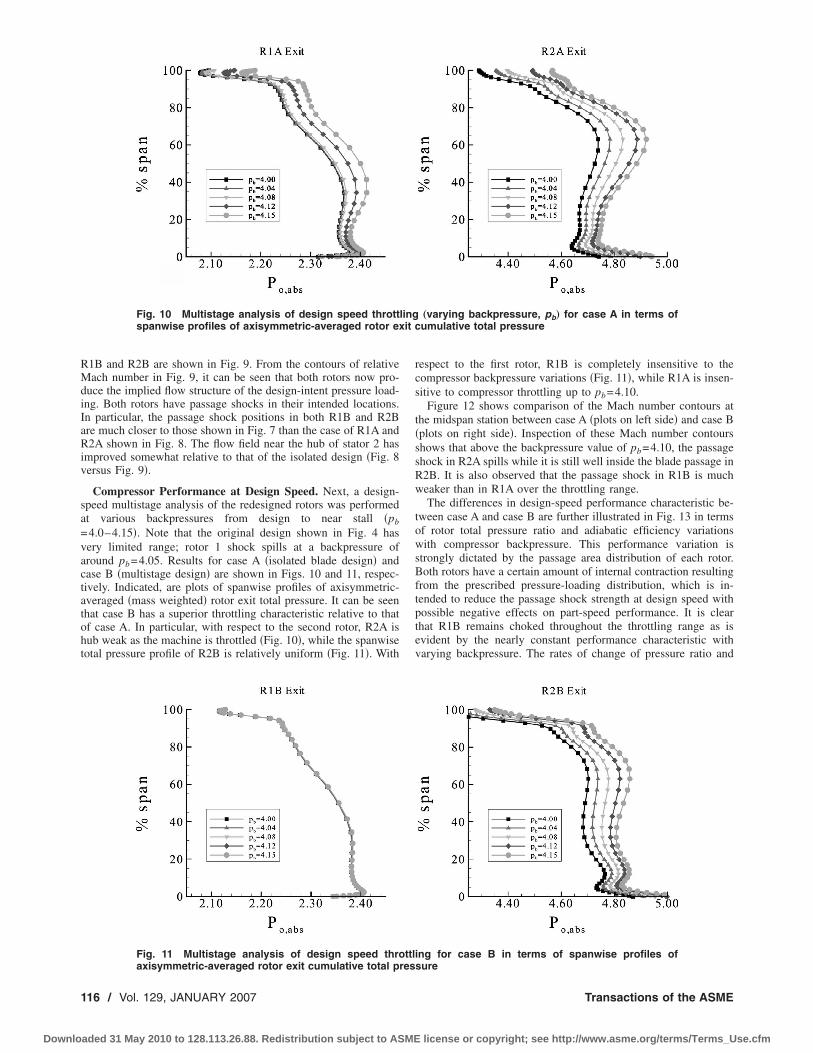
R1B and R2B are shown in Fig. 9. From the contours of relativeMach number in Fig. 9, it can be seen that both rotors now pro-duce the implied flow structure of the design-intent pressure load-ing. Both rotors have passage shocks in their intended locations.In particular, the passage shock positions in both R1B and R2Bare much closer to those shown in Fig. 7 than the case of R1A andR2A shown in Fig. 8. The flow field near the hub of stator 2 hasimproved somewhat relative to that of the isolated design �Fig. 8versus Fig. 9�.

Compressor Performance at Design Speed. Next, a design-speed multistage analysis of the redesigned rotors was performedat various backpressures from design to near stall �pb

=4.0–4.15�. Note that the original design shown in Fig. 4 hasvery limited range; rotor 1 shock spills at a backpressure ofaround pb=4.05. Results for case A �isolated blade design� andcase B �multistage design� are shown in Figs. 10 and 11, respec-tively. Indicated, are plots of spanwise profiles of axisymmetric-averaged �mass weighted� rotor exit total pressure. It can be seenthat case B has a superior throttling characteristic relative to thatof case A. In particular, with respect to the second rotor, R2A ishub weak as the machine is throttled �Fig. 10�, while the spanwisetotal pressure profile of R2B is relatively uniform �Fig. 11�. With

respect to the first rotor, R1B is completely insensitive to thecompressor backpressure variations �Fig. 11�, while R1A is insen-sitive to compressor throttling up to pb=4.10.

Figure 12 shows comparison of the Mach number contours atthe midspan station between case A �plots on left side� and case B�plots on right side�. Inspection of these Mach number contoursshows that above the backpressure value of pb=4.10, the passageshock in R2A spills while it is still well inside the blade passage inR2B. It is also observed that the passage shock in R1B is muchweaker than in R1A over the throttling range.

The differences in design-speed performance characteristic be-tween case A and case B are further illustrated in Fig. 13 in termsof rotor total pressure ratio and adiabatic efficiency variationswith compressor backpressure. This performance variation isstrongly dictated by the passage area distribution of each rotor.Both rotors have a certain amount of internal contraction resultingfrom the prescribed pressure-loading distribution, which is in-tended to reduce the passage shock strength at design speed withpossible negative effects on part-speed performance. It is clearthat R1B remains choked throughout the throttling range as isevident by the nearly constant performance characteristic withvarying backpressure. The rates of change of pressure ratio and

Fig. 10 Multistage analysis of design speed throttling „varying backpressure, pb… for case A in terms ofspanwise profiles of axisymmetric-averaged rotor exit cumulative total pressure

Fig. 11 Multistage analysis of design speed throttling for case B in terms of spanwise profiles ofaxisymmetric-averaged rotor exit cumulative total pressure



efficiency with backpressure for the two cases are very differentindicating a superior design point blade row matching potentialfor case B. Assessment of the aero-stability of the 2.5 stage is

computationally difficult and is subject to many uncertainties thatare beyond the scope of this analysis. Heuristically, it would seemthat R2B has a lager peak pressure rise potential than R2A, whichdoes not necessarily imply a more favorable compressor in termsof ultimate throttling range. Finally, Fig. 14 shows that case B alsoexhibits a slight increase in adiabatic efficiency over the applieddesign-speed throttling range when compared to case A, on theorder of 0.3%. Figure 14 indicates that for both case A and case B,the design requirement of an overall compression ratio of 4.65:1at a backpressure of 4.0 is nearly satisfied.

In summary, this exercise shows that by using the newly imple-mented multistage inverse method, the resulting rotor blade de-signs �design case B� produce pressure-loading distributionscloser to design-intent than when using the isolated blade rowinverse method �design case A�. The rotor blades designed usingthe multistage method also exhibit a more desirable design-speedthrottling characteristic. Whether or not this leads to a more fa-vorable aerostability characteristic requires further careful inves-tigation.

ConclusionsAn existing three-dimensional inverse blading design code,

INV3D, has been successfully extended to handle multistage blad-ing design and analysis via a steady averaging-plane blade rowcoupling scheme. The extended code has been successfully ap-plied to redesign exercises involving a highly loaded 2.5-stageaxial compressor.

It has been shown that multiple blades can be redesigned simul-taneously in their mutually interacting environments with a mod-est increase in computational cost. Furthermore, the viability of

Fig. 12 Multistage analysis of design speed throttling for case A „left… and case B „right… interms of relative Mach number contour at midspan for different backpressures

Fig. 13 Multistage analysis of design speed throttling forcases A and B. Shown are throttling characteristics of the re-spective rotors 1 and rotors 2 within the 2.5 stage.



inverse blading design for the purpose of enhanced design pointaeromatching of multistage compressors has been demonstrated.This has the potential to greatly facilitate the process of blade rowmatching during design iterations, and is a significant improve-ment over existing approaches used to address design point aero-dynamic matching.

Many more issues need to be addressed before this inversedesign scheme can be successfully deployed in the future designsystem proposed herein. Noteworthy, is the need for a pressure-loading regulation scheme that automatically adjusts the pressure-loading distribution and magnitude in order to meet the requiredaxisymmetric-averaged design intent static pressure field. It ishoped that the present investigation will serve to motivate furtherresearch.

AcknowledgmentThis work was partially funded by NASA Glenn Research Cen-

ter for whose support the authors are grateful.

References�1� Adamczyk, J. J., 2000, “Aerodynamic Analysis of Multistage Turbomachinery

Flows in Support of Aerodynamic Design,” ASME J. Turbomach., 122, pp.189–217.

�2� Gallimore, S. J., 1999, “Axial Flow Compressor Design,” Developments inTurbomachinery Design, J. Denton, ed., American Institution of MechanicalEngineers.

�3� Marble, F. E., 1964, “Three-Dimensional Flow in Turbomachines,” HighSpeed Aerodynamics and Jet Propulsion, Vol. X, Aerodynamics of Turbines andCompressors, W. R. Hawthorne, ed., Princeton University Press, Princeton,NJ, pp. 83–165.

�4� Dang, T. Q., 1995, ‘ ‘Inverse Method for Turbomachine Blades Using Shock-Capturing Techniques,” AIAA Paper No. 95-2465.

�5� Qiu, X., 1999, “Improved Algorithm for Three-Dimensional Inverse Method,”Ph.D. dissertation, Department of Mechanical Engineering, Syracuse Univer-sity, Syracuse, NY.

�6� Damle, S., Dang, T., Stringham, J., and Razinsky, E., 1999, “Practical Use ofa 3D Viscous Inverse Method for the Design of Compressor Blade,” ASME J.Turbomach., 121�2�, pp. 321–325.

�7� Qiu, X., and Dang, T., 2000, “3D Inverse Method for Turbomachine BladingWith Splitter Blades,” ASME Paper No. 2000-GT-526.

�8� Dang, T., Damle, S., and Qiu, X., 2000, “Euler-Based Inverse Method forTurbomachine Blades: Part II—Three Dimensions,” AIAA J., 38�11�, pp.2007–2013.

�9� Medd, A. J., 2002, “Enhanced Inverse Design Code and Development of De-sign Strategies for Transonic Compressor Blading,” Ph.D. dissertation, Depart-ment of Mechanical Engineering, Syracuse University, Syracuse, NY.

�10� Jameson, A., Schmidt, W., and Turkel, E., 1981, “Numerical Solution of theEuler Equations by Finite Volume Methods Using Runge-Kutta Time-SteppingSchemes,” AIAA Paper No. 81-1259.

�11� Denton, J. D., 1992, “The Calculation of Three Dimensional Viscous FlowThrough Multistage Turbomachines,” ASME J. Turbomach., 114, pp. 18–26.

�12� Wadia, A. R., and Beacher, B. F., 1990, “Three-Dimensional Relief in Turbo-machinery Blading,” ASME J. Turbomach., 112, pp. 587–598.

�13� Reid, L., and Moore, R. D., 1978, “Design and Overall Performance of FourHighly-Loaded, High-Speed Inlet Stages for an Advanced, High-Pressure-Ratio Core Compressor,” NASA TP-1337.

�14� Reid, L., and Moore, R. D., 1980, “Experimental Study of Low Aspect RatioCompressor Blading,” ASME Paper No. 80-GT-6.

�15� Hall, E. J., and Delaney, R. A., 1995, “Investigation of Advanced Counterro-tation Blade Configuration Concepts for High Speed Turboprop Systems: TaskVII-ADPAC User’s Manual,” NASA CR-195472.

�16� Dawes, W. N., 1992, “Toward Improved Throughflow Capability: The Use ofThree-Dimensional Viscous Flow Solvers in a Multistage Environment,”ASME J. Turbomach., 114, pp. 8–17.

�17� Chima, R. V., 1998, “Calculation of Multistage Turbomachinery Using SteadyCharacteristic Boundary Conditions,” NASA Technical Memorandum, No.206613.

�18� Giles, M. B., 1990, “Nonreflecting Boundary Conditions for Euler EquationCalculations,” AIAA J., 28, pp. 2050–2058.

�19� Gropp, W., Lusk, E., Doss, N., and Skjellum, A., 1996, “A High-Performance,Portable Implementation of the MPI Message Passing Interface Standard,”Parallel Comput., 22, pp. 789–828.

�20� Gropp, W. D., and Lusk, E., 1996, “Guide for a Portable Implementation ofMPI,” ANL-96/6, Mathematics and Computer Science Division, Argonne Na-tional Laboratory.

�21� Larosiliere, L. M., Wood, J. R., Hathaway, M. D., Medd, A. J., and Dang, T.Q., 2002, “Aerodynamic Design Study of an Advanced Multistage Axial Com-pressor,” NASA TP-211568.

�22� Medd, A. J., Dang, T. Q., and Larosiliere, L. M., 2003, “3D Inverse DesignLoading Strategy for Transonic Axial Compressor Blading,” ASME Paper No.2003-GT-38501.

Fig. 14 Multistage analysis of design speed throttling for cases A and B. Shown are thethrottling characteristics of the complete 2.5 stages.



Elisabet SyverudDepartment of Energy and Process Engineering,

NTNU,Norwegian University of Science and Technology,

Trondheim, Norway

Olaf BrekkeRoyal Norwegian Navy,

Bergen, Norway

Lars E. BakkenDepartment of Energy and Process Engineering,

NTNU,Norwegian University of Science and Technology,

Trondheim, Norway

Axial Compressor DeteriorationCaused by Saltwater IngestionGas turbine performance deterioration can be a major economic factor. An example iswithin offshore installations where a degradation of gas turbine performance can mean areduction of oil and gas production. This paper describes the test results from a series ofaccelerated deterioration tests on a General Electric J85-13 jet engine. The axial com-pressor was deteriorated by spraying atomized droplets of saltwater into the engineintake. The paper presents the overall engine performance deterioration as well as de-teriorated stage characteristics. The results of laboratory analysis of the salt deposits arepresented, providing insight into the increased surface roughness and the deposit thick-ness and distribution. The test data show good agreement with published stage charac-teristics and give valuable information regarding stage-by-stage performancedeterioration. �DOI: 10.1115/1.2219763�

IntroductionCompressor fouling causes 70–85% of the performance loss

due to deterioration in gas turbines �1�. The degradation rate willbe affected by site-specific conditions of the fouling and by engineoperating conditions. A thorough review of engine performancedeterioration mechanisms and modeling is given by Kurz andBrun �2�.

From operating experience and literature the first stages of anaxial compressor are expected to be the ones most heavily fouled.Deposits will have different characteristics depending on the na-ture of the fouling. Dry particles in dry atmospheres are likely todeposit in different areas compared to sticky matters and oilycompounds. At high inlet humidity, the drop in static pressureduring acceleration will increase the dust adhesion on the blades�3,4�.

To understand and reveal the degradation and restorationmechanisms related to recoverable compressor deterioration, asystematic test campaign has been performed on a General Elec-tric �GE� J85-13 jet engine. The overall performance of the gasturbine and compressor stage characteristics were analyzed in de-tail. The tests reflect actual performance deterioration as found inoffshore applications and provide valuable information regardingoverall and stage-by-stage compressor performance deteriorationin a real engine.

The tests were part of a larger online water wash test program.The results from this program are reported in a different paper �5�which should be seen in context with the present work.

Test Facilities and Engine DescriptionThe GE J85-13 engine has been a successful engine in different

applications since it first entered service in 1960. More than 6000of these engines are still in service worldwide. The Royal Norwe-gian Air Force �RNoAF� F-5 Freedom Fighters have two GEJ85-13 engines for propulsion. Because these aircrafts have beenreplaced by the F-16 aircraft, one GE J85-13 engine has beenmade available to the Norwegian University of Science and Tech-nology for use in this project. Engine testing was carried out at theRNoAF’s test facilities at Kjeller, Norway. Kjeller is located in-land, �25 km east of Oslo at an altitude of 119 m above sea level.

The GE J85-13 is a compact, light-weight, single-spool turbojetengine. It has an eight-stage axial-flow compressor that is directly

coupled to a two-stage turbine. The exhaust nozzle has a variablethroat area, and the engine is equipped with an afterburner. TheGE J85-13 is rated to deliver a minimum thrust of 2720 lb�12.1 kN� at 100% shaft speed without the afterburner and a mini-mum thrust of 4080 lb �18.1 kN� with full afterburner.

The eight-stage compressor has a pressure ratio of 6.5:1. First-and second-stage rotor blades are coated for corrosion protection.To handle off-design operation, the compressor has variable inletguide vanes �IGV� and bleed-off-valves at stages 3–5, as well as avariable exhaust nozzle. The variable geometry is controlled bythe throttle angle, but the timing is ambient temperature biased. AtISO conditions, IGV will be at maximum deflection and bleed-off-valves will be fully open below �81% corrected speed andfully closed at �96% corrected speed. At ambient temperaturesabove ISO conditions, the bleed-off-valves will close at lowerspeed settings. The nozzle is controlled by the throttle as long asthe engine is running below the exhaust temperature limit. Whenthe maximum exhaust temperature is reached, the exhaust nozzlewill open to increase the exhaust flow. This reversal in the exhaustnozzle schedule occurs close to the maximum throttle angle.

Bleed air is also used for internal cooling of the afterburneractuators, combustor liner, and turbine guide vanes. Bleed air foranti-ice is taken at the compressor discharge. The anti-ice airvalve was kept closed during all tests associated with this project.

Engine Model Data. Detailed knowledge of compressor stagegeometry is available through several sources providing a goodbasis for developing engine simulation models.

NASA carried out several tests on the GE J85-13 in the late1960s and throughout the 1970s, and reported compressor stagetemperature and pressure profiles �6�, individual compressor stagecharacteristics �7,8� as well as gas path geometry �9�.

Initial Engine Condition. The engine used in this test programwas preserved and stored after serving �300 h onboard an air-craft. The engine was not overhauled prior to testing.

To avoid disturbances to the airflow attributable to loose coat-ing, the coating on the second-stage rotor blades was removed byhand prior to the testing, using emery paper grade 320. The com-pressor inlet, inlet guide vanes, first-stage rotor, and stator werecleaned by hand using solvent, while the upper half of the casing,including stator vanes from stages 1 to 7 were cleaned using anultrasonic cleaning bath. In addition, online compressor cleaningwas performed prior to the testing using water at a flow of13.2 l /min, for a 30 second period at idle, 70%, 90%, 95%, and100% corrected engine speed. Details of the online water washsystem are given in a different paper �5�.




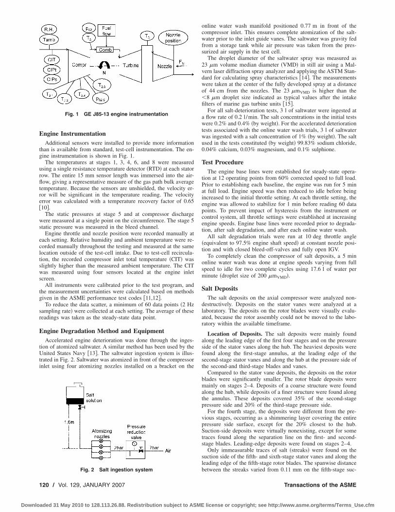
Engine InstrumentationAdditional sensors were installed to provide more information

than is available from standard, test-cell instrumentation. The en-gine instrumentation is shown in Fig. 1.

The temperatures at stages 1, 3, 4, 6, and 8 were measuredusing a single resistance temperature detector �RTD� at each statorrow. The entire 15 mm sensor length was immersed into the air-flow, giving a representative measure of the gas path bulk averagetemperature. Because the sensors are unshielded, the velocity er-ror will be significant in the temperature reading. The velocityerror was calculated with a temperature recovery factor of 0.65�10�.

The static pressures at stage 5 and at compressor dischargewere measured at a single point on the circumference. The stage 5static pressure was measured in the bleed channel.

Engine throttle and nozzle position were recorded manually ateach setting. Relative humidity and ambient temperature were re-corded manually throughout the testing and measured at the samelocation outside of the test-cell intake. Due to test-cell recircula-tion, the recorded compressor inlet total temperature �CIT� wasslightly higher than the measured ambient temperature. The CITwas measured using four sensors located at the engine inletscreen.

All instruments were calibrated prior to the test program, andthe measurement uncertainties were calculated based on methodsgiven in the ASME performance test codes �11,12�.

To reduce the data scatter, a minimum of 60 data points �2 Hzsampling rate� were collected at each setting. The average of thesereadings was taken as the steady-state data point.

Engine Degradation Method and EquipmentAccelerated engine deterioration was done through the inges-

tion of atomized saltwater. A similar method has been used by theUnited States Navy �13�. The saltwater ingestion system is illus-trated in Fig. 2. Saltwater was atomized in front of the compressorinlet using four atomizing nozzles installed on a bracket on the

online water wash manifold positioned 0.77 m in front of thecompressor inlet. This ensures complete atomization of the salt-water prior to the inlet guide vanes. The saltwater was gravity fedfrom a storage tank while air pressure was taken from the pres-surized air supply in the test cell.

The droplet diameter of the saltwater spray was measured as23 �m volume median diameter �VMD� in still air using a Mal-vern laser diffraction spray analyzer and applying the ASTM Stan-dard for calculating spray characteristics �14�. The measurementswere taken at the center of the fully developed spray at a distanceof 44 cm from the nozzles. The 23 �mVMD is higher than the�8 �m droplet size indicated as typical values after the intakefilters of marine gas turbine units �15�.

For all salt-deterioration tests, 3 l of saltwater were ingested ata flow rate of 0.2 l /min. The salt concentrations in the initial testswere 0.2% and 0.4% �by weight�. For the accelerated deteriorationtests associated with the online water wash trials, 3 l of saltwaterwas ingested with a salt concentration of 1% �by weight�. The saltused in the tests constituted �by weight� 99.83% sodium chloride,0.04% calcium, 0.03% magnesium, and 0.1% sulphione.

Test ProcedureThe engine base lines were established for steady-state opera-

tion at 12 operating points from 60% corrected speed to full load.Prior to establishing each baseline, the engine was run for 5 minat full load. Engine speed was then reduced to idle before beingincreased to the initial throttle setting. At each throttle setting, theengine was allowed to stabilize for 1 min before reading 60 datapoints. To prevent impact of hysteresis from the instrument orcontrol system, all throttle settings were established at increasingengine speeds. Engine base lines were recorded prior to degrada-tion, after salt degradation, and after each online water wash.

All salt degradation trials were run at 10 deg throttle angle�equivalent to 97.5% engine shaft speed� at constant nozzle posi-tion and with closed bleed-off-valves and fully open IGV.

To completely clean the compressor of salt deposits, a 5 minonline water wash was done at engine speeds varying from fullspeed to idle for two complete cycles using 17.6 l of water perminute �droplet size of 200 �mVMD�.

Salt DepositsThe salt deposits on the axial compressor were analyzed non-

destructively. Deposits on the stator vanes were analyzed at alaboratory. The deposits on the rotor blades were visually evalu-ated, because the rotor assembly could not be moved to the labo-ratory within the available timeframe.

Location of Deposits. The salt deposits were mainly foundalong the leading edge of the first four stages and on the pressureside of the stator vanes along the hub. The heaviest deposits werefound along the first-stage annulus, at the leading edge of thesecond-stage stator vanes and along the hub at the pressure side ofthe second-and third-stage blades and vanes.

Compared to the stator vane deposits, the deposits on the rotorblades were significantly smaller. The rotor blade deposits weremainly on stages 2–4. Deposits of a coarse structure were foundalong the hub, while deposits of a finer structure were found alongthe annulus. These deposits covered 35% of the second-stagepressure side and 20% of the third-stage pressure side.

For the fourth stage, the deposits were different from the pre-vious stages, occurring as a shimmering layer covering the entirepressure side surface, except for the 20% closest to the hub.Suction-side deposits were virtually nonexisting, except for sometraces found along the separation line on the first- and second-stage blades. Leading-edge deposits were found on stages 2–4.

Only immeasurable traces of salt �streaks� were found on thesuction side of the fifth- and sixth-stage stator vanes and along theleading edge of the fifth-stage rotor blades. The spanwise distancebetween the streaks varied from 0.11 mm on the fifth-stage suc-

Fig. 1 GE J85-13 engine instrumentation

Fig. 2 Salt ingestion system



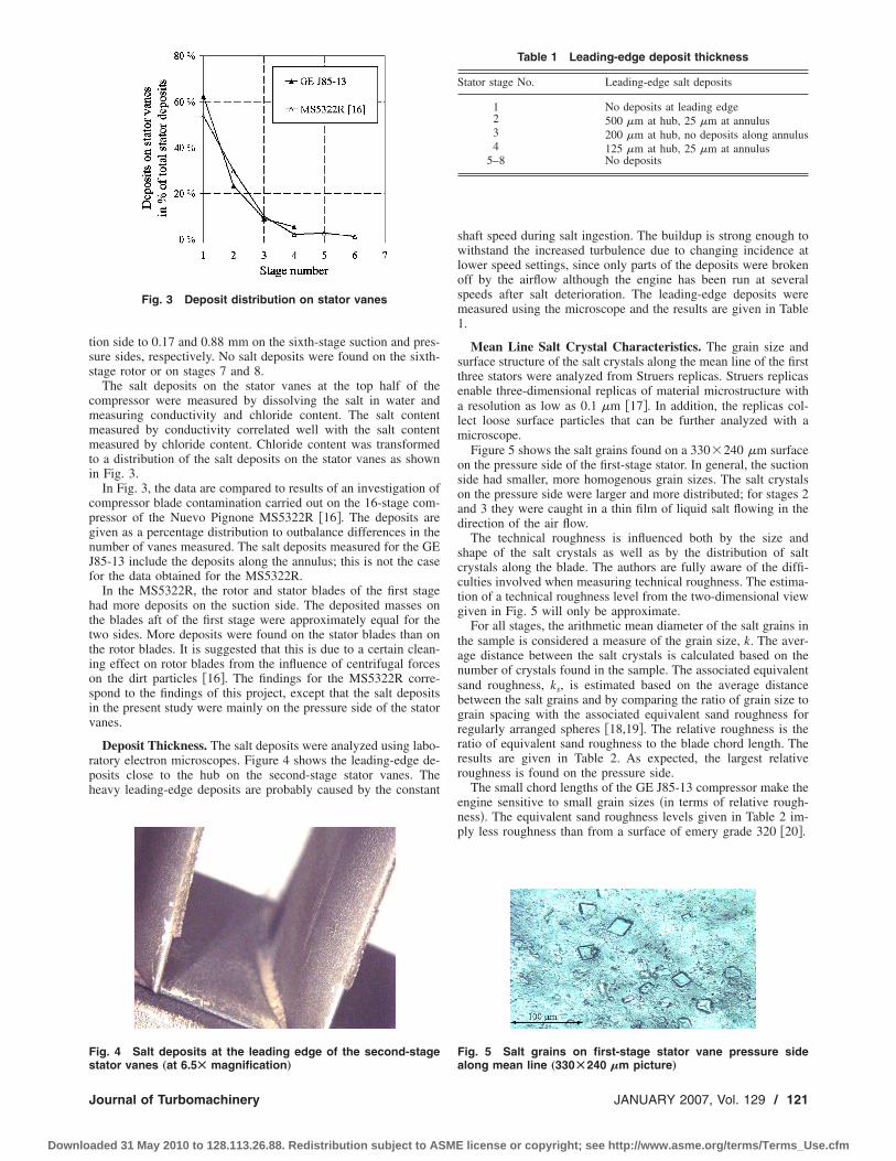
tion side to 0.17 and 0.88 mm on the sixth-stage suction and pres-sure sides, respectively. No salt deposits were found on the sixth-stage rotor or on stages 7 and 8.

The salt deposits on the stator vanes at the top half of thecompressor were measured by dissolving the salt in water andmeasuring conductivity and chloride content. The salt contentmeasured by conductivity correlated well with the salt contentmeasured by chloride content. Chloride content was transformedto a distribution of the salt deposits on the stator vanes as shownin Fig. 3.

In Fig. 3, the data are compared to results of an investigation ofcompressor blade contamination carried out on the 16-stage com-pressor of the Nuevo Pignone MS5322R �16�. The deposits aregiven as a percentage distribution to outbalance differences in thenumber of vanes measured. The salt deposits measured for the GEJ85-13 include the deposits along the annulus; this is not the casefor the data obtained for the MS5322R.

In the MS5322R, the rotor and stator blades of the first stagehad more deposits on the suction side. The deposited masses onthe blades aft of the first stage were approximately equal for thetwo sides. More deposits were found on the stator blades than onthe rotor blades. It is suggested that this is due to a certain clean-ing effect on rotor blades from the influence of centrifugal forceson the dirt particles �16�. The findings for the MS5322R corre-spond to the findings of this project, except that the salt depositsin the present study were mainly on the pressure side of the statorvanes.

Deposit Thickness. The salt deposits were analyzed using labo-ratory electron microscopes. Figure 4 shows the leading-edge de-posits close to the hub on the second-stage stator vanes. Theheavy leading-edge deposits are probably caused by the constant

shaft speed during salt ingestion. The buildup is strong enough towithstand the increased turbulence due to changing incidence atlower speed settings, since only parts of the deposits were brokenoff by the airflow although the engine has been run at severalspeeds after salt deterioration. The leading-edge deposits weremeasured using the microscope and the results are given in Table1.

Mean Line Salt Crystal Characteristics. The grain size andsurface structure of the salt crystals along the mean line of the firstthree stators were analyzed from Struers replicas. Struers replicasenable three-dimensional replicas of material microstructure witha resolution as low as 0.1 �m �17�. In addition, the replicas col-lect loose surface particles that can be further analyzed with amicroscope.

Figure 5 shows the salt grains found on a 330�240 �m surfaceon the pressure side of the first-stage stator. In general, the suctionside had smaller, more homogenous grain sizes. The salt crystalson the pressure side were larger and more distributed; for stages 2and 3 they were caught in a thin film of liquid salt flowing in thedirection of the air flow.

The technical roughness is influenced both by the size andshape of the salt crystals as well as by the distribution of saltcrystals along the blade. The authors are fully aware of the diffi-culties involved when measuring technical roughness. The estima-tion of a technical roughness level from the two-dimensional viewgiven in Fig. 5 will only be approximate.

For all stages, the arithmetic mean diameter of the salt grains inthe sample is considered a measure of the grain size, k. The aver-age distance between the salt crystals is calculated based on thenumber of crystals found in the sample. The associated equivalentsand roughness, ks, is estimated based on the average distancebetween the salt grains and by comparing the ratio of grain size tograin spacing with the associated equivalent sand roughness forregularly arranged spheres �18,19�. The relative roughness is theratio of equivalent sand roughness to the blade chord length. Theresults are given in Table 2. As expected, the largest relativeroughness is found on the pressure side.

The small chord lengths of the GE J85-13 compressor make theengine sensitive to small grain sizes �in terms of relative rough-ness�. The equivalent sand roughness levels given in Table 2 im-ply less roughness than from a surface of emery grade 320 �20�.

Fig. 3 Deposit distribution on stator vanes

Fig. 4 Salt deposits at the leading edge of the second-stagestator vanes „at 6.5Ã magnification…

Table 1 Leading-edge deposit thickness

Stator stage No. Leading-edge salt deposits

1 No deposits at leading edge2 500 �m at hub, 25 �m at annulus3 200 �m at hub, no deposits along annulus4 125 �m at hub, 25 �m at annulus

5–8 No deposits

Fig. 5 Salt grains on first-stage stator vane pressure sidealong mean line „330Ã240 �m picture…



Significance of Salt Deposits on Compressor Perfor-mance Characteristics

The effect of Reynolds number on compressor performance iswell known for compressors in new and clean conditions. TheASME test code on compressors �21� does not give any attentionto testing in deteriorated conditions. A study of Reynolds numbereffects in centrifugal compressors shows how efficiency can becorrelated to increases in the friction factor with increased surfaceroughness �22�. Some research exists on the effect of increasedroughness in axial compressors: A study of profile loss due tosurface roughness on NACA 65-12�06� profiles showed a 2% in-crease in the profile losses at a relative roughness �ks/chord� of3E-4 and a 10% increase at 50E-4 �2�. Another study showed a9% reduction in the static pressure ratio at a relative roughness of10E-4, but the static pressure ratio is a strong function of thevolume flow and blade velocity �20�. The effect of surface rough-ness on blade profile loss is quantified through a momentum thick-ness correlation �23�. Additional insight is given into the boundarylayer characterization of rough surfaces, although applied to newand clean surfaces �19�.

The critical roughness Reynolds number, defined in Eq. �1��19�, is independent of the characteristic length of the compressor

Recritical =ksV

��1�

When the critical Reynolds number is above 90, the flow can beassumed hydrodynamically rough with turbulent attached flow�i.e., with the salt crystals protruding into the laminar sublayer�.For these cases, the associated blade profile loss will dependsolely on the surface roughness to chord level, and not on thechord Reynolds number �19�.

Applying Eq. �1� to the GE J85-13, a critical Reynolds numberof 90 implies a maximum equivalent sand roughness of 5 �m.Table 2 shows the salt crystals have equivalent sand roughnesslevels above 5 �m for all stages except the suction side of stagethree stator vanes. This implies that the blade loss, hence, theefficiency, of the deteriorated engine will be dependent on theroughness level and not on the chord Reynolds number. Thechange in stage efficiency should therefore be possible to calcu-late based on the correlation for momentum thickness with surfaceroughness �23�.

Another aspect of the increased surface roughness is the changein deviation angle due to the thickening of the blade boundarylayer. A correlation for changes in the deviation angle due to sur-face roughness is found from tests of a helicopter engine after1500 h of flight �24�. The relative roughness levels reported werein the range of 10.9E-3 in the first stage to 0.7�10E-3 in the laststage and at Reynolds numbers of 240,000. Typical Reynoldsnumbers in the GE J85-13 are 200,000 to 600,000; however, therelative roughness level given in Table 2 is only one tenth of thelevel reported for the helicopter engine �24�. Therefore, changes tothe deviation angle due to deterioration are considered negligiblefor the salt-deteriorated GE J85-13.

Engine Performance DeteriorationThe engine deterioration due to salt deposits is analyzed in the

following section. All overall engine performance parameters pre-sented are corrected to ISO reference conditions �25�. Variationsin humidity were not accounted for in the calculations. Datapoints measured at low speed settings were not included, becausethese include large unaccounted bleed flows.

Initial Salt Deterioration Trials. Figure 6 shows the resultsfrom the initial salt-deterioration testing, where salt was injectedin three separate tests without water wash in between. The figureshows the total mass of salt ingested in the tests. The overallengine performance deterioration is shown for intake depression,which is defined as the difference between the total and staticpressure in the bellmouth throat. The intake depression deterio-rates rapidly and is outside of the measurement uncertainty toler-ance even after 6 g of salt ingestion. The intake depression wasthe most sensitive parameter to compressor deterioration and wasfound to be the best method for condition monitoring of the en-gine, because it is less dependent of the engine control mode.

Overall Engine Performance Deterioration. The engine per-formance deterioration with 30 g of salt ingested is shown in Figs.7–10. For simplicity in the presentation of data, only two repre-sentative cases are shown. These cases were recorded on the sameday at identical compressor variable geometry and nozzle posi-tions. Because the testing was done at ambient temperatures abovethe ISO reference condition, the 100% corrected speed setting wasnever reached. At these high ambient temperatures, the bleed-offvalves are fully closed above 95% corrected speed.

Figure 7 shows the engine performance deterioration in termsof changes on the compressor equilibrium operating line. Thestatic-to-total compressor pressure ratio is given at stage 5 �station2.5� and at compressor discharge �station 3�; both parameters are

Table 2 Salt crystal grain size and distribution at mean line

Statorvane

Mean grainsize, k��m�

Mean graindistance

��m�Equivalent sand roughness,

ks ��m�

Relativeroughness,ks / chord

1 PS 22 88 25 11E-41 SS 14 88 10 4E-42 PS 16 62 20 11E-42 SS 8 25 15 8E-43 PS 15 65 15 10E-43 SS 5 40 2 0.6E-4

Fig. 6 Deterioration of intake depression

Fig. 7 Effect of deterioration on compressor operating line



related to the total inlet pressure. Deterioration shifts the compres-sor operating line to a lower flow rate and a lower pressure ratio.Similar percentage changes to the compressor pressure ratio arefound at both stations, indicating that the pressure deteriorationwas at the front end of the compressor. Front stage fouling isknown to cause larger changes in the flow rate than in the pressurecapability �3�, and the results of Fig. 7 are in agreement with this.

The surge line is not known for the engine; however, surge wasnot encountered at any time during the test.

Figure 8 shows the change in exhaust gas temperature withthrust. The exhaust gas temperature is approximately nine percent-age points higher for the deteriorated engine. The flattening of thedeteriorated engine curve at the high end is due to exhaust gastemperature limitations in the engine control.

The variation in compressor isentropic efficiency with correctedengine shaft speed is shown in Fig. 9. This figure shows that

deterioration reduces the isentropic efficiency by approximatelythree percentage points along the operating line, and reduces theengine operating speed. In addition, the isentropic efficiency curveis flattened when the maximum exhaust gas temperature isreached.

The variation in compressor mass flow rate with engine shaftspeed is shown in Fig. 10. This figure shows the significant reduc-tion in air flow rate for the deteriorated engine. Again, the dete-riorated engine performance is shifted to a lower shaft speed;however, the mass flow rate is only slightly affected by the ex-haust gas temperature limitation. Mass flow rate is directly relatedto the intake depression which was found as the best parameter forengine condition monitoring in the initial salt deterioration trials.

Stage Work Coefficient DeteriorationThe compressor temperature measurements allow for a close

look at the stage work coefficient during salt deterioration. Thepresented test data are limited to engine operation above 95%engine shaft speed where the engine bleed-off-valves were closedand the IGV fully open.

The following assumptions are made when analyzing the testdata:

• The temperatures were measured at stages 1, 3, 4, 6, and 8,and a linear temperature distribution was used for the re-maining stages. The stage temperatures were measured inthe stator; however, the measurements were assumed to bevalid at the stator outlet plane.

• The temperature dependence of the specific heat at constantpressure and the ratio of specific heats are defined by afifth-order polynomial correlation for dry air �26� and aseventh-order polynomial for water vapor �25�. These poly-nomial correlations fit original data within 0.1% at the tem-perature range applicable to the GE J85-13.

• Air is assumed to be a thermally perfect gas, but with hu-midity included in the calculation of R, cp, and � as de-scribed in Appendix A. With an engine pressure ratio of6.5:1, this implies a 0.3% error compared to the results us-ing the Redlich-Kwong correlation for humid air mixtures�27� in the range of temperatures and pressures applicable tothe GE J85-13 axial compressor.

• The axial velocity is assumed constant from rotor inlet torotor outlet in a stage.

• The stage pressure rise is found from the measured poly-tropic efficiency.

• The stator deviation angle is assumed constant independentof incidence angle or corrected speed �9�. Increased devia-tion due to surface roughness is neglected as discussedabove.

• The discharge coefficient of the bellmouth is assumed to be0.98.

• The pressure loss in the IGV is assumed negligible. For thedata presented, the fully open IGV will not cause any turn-ing of the flow.

• Deterioration is assumed to increase the sidewall boundarylayers due to deposits on the first-stage annulus. The result-ing decrease in effective flow area is modeled through ablockage factor defined as the ratio of true flow area togeometrical flow area. Assuming no deviation of the eight-stage flow coefficient for the deteriorated engine comparedto clean conditions, the deteriorated engine blockage factorwas found to be 0.96. The blockage factor is assumed con-stant for all stages.

• The equations used to calculate stage performance are givenin Appendix B.

The test data are compared to the theoretical work coefficientbased on the engine geometry and the stage work coefficientfound in literature �7�.

Fig. 8 Change in exhaust gas temperature with thrust

Fig. 9 Deterioration of compressor isentropic efficiency

Fig. 10 Deterioration of compressor mass flow



The theoretical work coefficient is defined from the Euler tur-bine equation, Eq. �2� �28�

�theoreticalT = 1 − ��tan�1� + tan�2�� 2�

where 1 is the exit angle from the preceding stator and 2 is theexit blade angle �relative� from the rotor.

The data published on the stage work coefficients are calculatedbased on constant values for cp �1.005 kJ/kg K� and � �1.4� �7�.In this paper, these gas properties are dependent on gas tempera-ture and humidity. The difference will be largest in the aft stageswhere the gas temperatures are at the highest. Still, the publisheddata gives a good indication of the GE J85-13 stage performancefor a large range of flow coefficients.

Figures 11–14 show the change in the stage work coefficientwith engine deterioration for stages 2–4 and 6. For stages 2–4,deterioration reduces both the stage work coefficient and the flowcoefficient. This was expected for a degraded stage. For stage 6,

the data for deteriorated engine and clean engine overlay eachother. The same trend is found in all stages 5–8, indicating zerofouling in the aft stages. This agrees well with the observation ofonly minor traces of salt deposits in stages 5 and 6 and no saltdeposits in stages 7 or 8.

The measurements are in good agreement with the publisheddata �7� for stages 2–4. However, for stage 6, the measured stagework coefficient is higher than the published data. Because thecurrent analysis is based on the difference between the clean anddeteriorated condition, this deviation from expected stage workcoefficient is of no consequence. The bellmouth discharge coeffi-cient and the temperature recovery factor will influence on thestage work and flow coefficients. These factors are kept constantin the analysis.

ConclusionsThe test results presented in this paper show deteriorated per-

formance of the GE J85-13 jet engine after accelerated salt-deterioration tests undertaken at the test facilities of the RoyalNorwegian Air Force. Accelerated salt testing was found to be aneffective method to systematically deteriorate gas turbine com-pressor performance.

Deposited matter in an engine will depend on the nature of thedeposits �i.e., the material, the particle size, and the adhesive ca-pability of the deposits�. With the present testing, the salt depositswere found mainly in the front stages of the compressor, and thestators were found to have more deposits than the rotor blades.The surface roughness levels and applicable Reynolds numberswere found to give added profile losses but no significant in-creases in the stator deviation angle.

The overall engine performance shows the difficulties involvedin condition monitoring of deteriorated engines, because the dete-rioration causes a nonlinear shift in the degraded performance.This hampers the comparison of deterioration trends based on thecalculation of percentage deviation at constant corrected enginespeed.

Intake depression was found to be the parameter most sensitiveto compressor deterioration. In addition, intake depression wasless influenced by the engine control mode.

The test data show good agreement with published data onincremental stage work and give valuable information of stage-by-stage engine performance deterioration. The salt deteriorationcaused an increase in the sidewall boundary layers and significantdeterioration in the stage characteristics of the first four stages.

This paper provides valuable information on stage performancedeterioration used in the evaluation of test data from online waterwash tests �5�.

AcknowledgmentThe project has been supported by Statoil ASA, Dresser-Rand

Norwegian Operations and the Royal Norwegian Navy. The Royal

Fig. 11 Stage 2 work coefficient






Norwegian Air Force is acknowledged for allowing access to theirtest facilities and for allowing us to borrow a GE J85-13 for testpurposes. Without the help of Hans K. Henriksen, a retired test-cell operator of the RNoAF, this project would never have cometo fruition.

NomenclatureA � effective flow area �m2�cp � specific heat at constant pressure �kJ/kg K�C � absolute air velocity �m/s�

CIT � compressor inlet temperature �K�CIP � compressor inlet pressure �kPa�

Comb � combustor �Fig. 1�Compr � compressor �Fig. 1�

EGT � exhaust gas temperature �Fig. 1�GE � General Electric

IGV � inlet guide vanesISO � International Organization for

Standardization1

k � grain size of salt crystals ��m�ks � equivalent sand roughness ��m�m � mass flow rate �kg/s�

MW � molecular weight �kg/kmole�N � shaft speed �rpm�

NACA � National Advisory Committee forAeronautics

NASA � National Aeronautics and SpaceAdministration

p � pressure �kPa�PS � pressure side �concave� of blades/ vanesR � gas constant �kJ/kg K�r � radius �m�

R0 � universal gas constant �kJ/kg K�Re � Reynolds number

R.H. � relative humidity �%�RNoAF � Royal Norwegian Air Force

RTD � resistance temperature detectorSS � suction side �convex� of blades and vanesStg � stage

T � temperature �K�U � blade velocity �m/s�V � relative air velocity �m/s�

VMD � volume median diameterwar � Specific humidity �kg H2O/kg dry air�

x � molar fraction of component

Greek Symbols � absolute air angle �deg� � relative air angle �deg�� air density �kg/m3� � efficiency� � kinematic viscosity �m2/s�� temperature recovery factor� � ratio of specific heats

�T=cp�Tt /Utip2 � stage work coefficient

�=Ca /Utip � flow coefficient

Subscriptsa � axial velocity component

amb � ambient conditionmix � mixture �humid air�poly � polytropic

s � static conditiont � total condition

tip � tip

VMD � volume median diameterw � tangential velocity component

2.1, 2.2,…, 2.7 � Compressor stage 1, 2,…, to stage 73 � Compressor discharge5 � Turbine discharge

Appendix A: Gas Properties for Humid AirGas properties for humid air are calculated from the following

correlations �25�

cp�mix = warmolarcp�H2O + �1 − warmolarcp�dry air�

�mix = warmolar�H2O + �1 − warmolar�dry air�

Rmix =R0

MWmix

MWmix = xH2OMWH2O + xdry airMWdry air

where warmolar=war�28.96/18.015�.

Appendix B: Stage Performance CalculationsConsider a stage where the rotor inlet, rotor outlet, and stator

outlet are designated as stations 1, 2, and 3, respectively. Theperformance of a single stage is calculated using the followingiterative sequence. The same sequence is used on all compressorstages.

�1� The following parameters are known at the rotor inlet: pt1,ps1, Tt1, Ts1, cp1, �1, and m.

�2� From the principle of conservation of mass and the assump-tion of a thermally perfect gas, the following parameters are cal-culated at the rotor inlet

�1 =ps1

RmixTs1, Ca1 =

m

�1A1

�3� The definition of total condition gives the absolute air ve-locity at the inlet

C1 = �2cp�mix�1�Tt1 − Ts1� , Cw1 = �C12 − Ca1

2

�4� The blade velocities at rotor inlet and outlet are given by theshaft rotation, where the radius, r, is the mean line radius forcalculation of velocity diagrams and the tip radius for calculationof stage work coefficient

U1 = 2�r1N

60, U2 = 2�r2

N

60

�5� To start the calculation loop, the static temperature at thestator outlet, Ts3, is given an initial value.

�6� The total temperature is calculated from the temperaturerecovery factor and the measured temperature, Tm

� =Tm − Ts

Tt − Ts⇒ Tt =

1/� �Tm − Ts� + Ts

1 − �

�7� All stage work is applied in the rotor row, hence, the totaltemperature will not change across the stator row

Cw2 =cp�mix�1�Tt2 − Tt1� + Cw1U1

U2

C2 = �Cw22 + Ca2

2

Ts2 = Tt2 −C2

2

2cp�mix�1

�8� Assuming constant axial velocity across the rotor row, Ca2=Ca1

1ISO reference conditions assume an ambient temperature of 288.15 K, a baro-metric pressure of 101.325 kPa and a relative humidity of 60%.



�2 =m

Ca1A2

ps2 = �2RmixTs2

pt2 = ps2� Tt2

Ts2��mix/��mix−1�

�9� The stage pressure rise is found from the measured poly-tropic efficiency and assumed constant in all stages

pt3 = pt1�Tt3

Tt1� poly�mix/��mix−1�

ps3 = pt3�Ts3

Tt3��mix/��mix−1�

�3 =ps3

RmixTs3

�10� The stator exit velocity is found assuming zero deviation inthe stator blade exit angle, 3=0

Ca3 =m

�3A3

C3 = Ca3 cos�3�

�11� Then, the value for cp�mix at the stator outlet is updatedbased on Ts3 and a new value for static temperature at the statoroutlet is calculated

Ts3 = Tt3 −C3

2

2cp�mix�3

�12� The calculations are repeated from step 6 and on using thevalue for Ts3 found in step 11, and the whole sequence is repeateduntil Ts3 converges.

References�1� Diakunchak, I. S., 1992, “Performance Degradation in Industrial Gas Tur-

bines,” ASME J. Eng. Gas Turbines Power, 114, pp. 161–168.�2� Kurz, R., and Brun, K., 2001, “Degradation in Gas Turbine Systems,” ASME

J. Eng. Gas Turbines Power, 123, pp. 70–77.�3� Zaba, T., 1980, “Losses in Gas Turbines Due to Deposits on the Blading,”

Brown Boveri Rev., 67�12�, pp. 715–722.�4� Meher-Homji, C. B., Chaker, M. A., and Motiwala, H., 2001, “Gas Turbine

Performance Deterioration,” Proceedings From the 30th Turbomachinery Sym-posium, Texas A&M, College Station, TX.

�5� Syverud, E., and Bakken, L. E., 2007, “Online Water Wash Test of GE J85-

13,” ASME J. Turbomach., 129�1�, pp. 136–142.�6� Hager, R. D., 1977, “Analysis of Internal Flow of J85-13 Multistage Compres-

sor,” NASA TM X-3513.�7� Milner, E. J., and Wenzel, L. M., 1975, “Performance of a J85-13 Compressor

With Clean and Distorted Inlet Flow,” NASA TM X-3304.�8� Willoh, R. G., and Seldner, K., 1969, “Multistage Compressor Simulation

Applied to the Prediction of Axial Flow Instabilities,” NASA TM X-1880.�9� Tesch, W. A., and Steenken, W. G., 1976, “Blade Row Dynamic Digital Com-

pressor Program: Volume 1 J85 Clean Inlet Flow and Parallel CompressorModels,” NASA CR-134978.

�10� AGARD, 1990, “Recommended Practices for Measurement of Gas Path Pres-sures and Temperatures for Performance Assessment of Aircraft Turbine En-gines and Components,” AGARD Advisory Report AR-245, H. I. H. Saravana-muttoo, ed., AGARD, Neuilly Sur Seine, France.

�11� ASME, 1997, Performance Test Code on Gas Turbines, ASME PTC 22-1997,ASME, New York.

�12� ASME, 1998, Test Uncertainty, ASME PTC 19.1-1998, ASME, New York.�13� Caguiat, D. E., Zipkin, D. M., and Patterson, J. S., 2002, “Compressor Fouling

Testing on Rolls Royce/Allison 501-K17 and General Electric LM2500 GasTurbine Engines,” ASME Paper No. GT2002-30262.

�14� ASTM, 1992, Standard Practice for Determining Data Criteria and Process-ing for Liquid Drop Size Analysis, ASTM E 799-92, ASTM International, WestConshohocken, PA.

�15� Caguiat, D. E., Connor, J., Duckless, E., and DeCorso, R. J., 2004, “Inlet AirSalt Concentration Detection on U.S. Navy Ship Service Gas Turbine Genera-tor Sets,” ASME Paper No. GT2004-53984.

�16� Tarabrin, W. P., Schurovsky, V. A., Bodrov, A. I., and Stalder, J.-P., 1998,“Influence of Axial Compressor Fouling on Gas Turbine Unit PerformanceBased on Different Schemes and With Different Initial Parameters,” ASMEPaper No. 98-GT-416.

�17� Struers RepliSet System, Struers A/S, Ballerup, Denmark, http://www.struers.com

�18� Schlichting, H., 1979, Boundary-Layer Theory, 7th ed., Mc Graw-Hill, NewYork.

�19� Schäffler, A., 1980, “Experimental and Analytical Investigation of the Effectsof Reynolds Number and Blade Surface Roughness on Multistage Axial FlowCompressors,” ASME J. Eng. Power, 102, pp. 5–13.

�20� Bammert, K., and Woelk, G. U., 1979, “The Influence of the Blading SurfaceRoughness on the Aerodynamic Behavior and Characteristic of an Axial Com-pressor,” ASME Paper No. 79-GT-102.

�21� ASME, 1997, ASME Performance Test Code on Compressors and Exhausters,ASME PTC 10, ASME, New York.

�22� International Compressed Air and Allied Machinery Committee, 1987, “Influ-ence of the Reynolds Number on the Performance of Centrifugal Compres-sors,” ASME Paper No. 87-GT-10.

�23� Koch, C. C., and Smith, L. H., 1979, “Loss Sources and Magnitudes in Axial-Flow Compressors,” ASME J. Eng. Power, 98, pp. 411–424.

�24� Mal’tsev, Yu. N., and Shakov, V. G., 1989, “Influence of Roughness of De-posits in Compressor Cascade on Flow Lag Angle �English Translation�,” Iz-vestiya VUZ, Aviatsionnaya Tekhnika, 32, pp. 80–82.

�25� Walsh, P. P., and Fletcher, P., 1998, Gas Turbine Performance, BlackwellScience, Oxford.

�26� Keenan, J. H., Chao, J., and Kaye, J., 1983, Gas Tables International Version,SI Units, 2nd ed., Wiley, New York.

�27� Aungier, R. H., 2003, “A Fast, Accurate Real Gas Equation of State for FluidDynamic Analysis Applications,” ASME J. Fluids Eng., 177, pp. 277–281.

�28� Saravanamuttoo, H. I. H., Rogers, G. F. C., and Cohen, H., 2001, Gas TurbineTheory, 5th ed., Prentice-Hall, Englewood Cliffs, NJ.



Matthew D. LangfordTechsburg, Inc.,

2901 Prosperity Road,Blacksburg, VA 24060


AndrewBreeze-Stringfellow

GE Aircraft Engines,1 Neumann Way,

Cincinnati, OH 45215e-mail: [email protected]

Stephen A. GuillotTechsburg, Inc.,

2901 Prosperity Road,Blacksburg, VA 24060


William SolomonGE Aircraft Engines,

1 Neumann Way,Cincinnati, OH 45215


Wing F. NgMechanical Engineering Department,

Virginia Tech,Blacksburg, VA 24060e-mail: [email protected]

Jordi EstevadeordalInnovative Scientific Solutions, Inc.,

2766 Indian Ripple Road,Dayton, OH 45440


Experimental Investigation of theEffects of a Moving Shock Waveon Compressor Stator FlowLinear cascade testing was performed to simulate the flow conditions experienced bystator blades in an axial compressor with supersonic relative Mach numbers at the inletto the downstream embedded rotors. Experiments were conducted in a transonic blow-down wind tunnel with a nominal inlet Mach number of 0.65. A single moving normalshock introduced at the exit of the stator cascade simulated the bow shock from a down-stream rotor. The shock was generated using a shock tube external to the wind tunnel.Pressure measurements indicated that the stator matched its design intent loading, turn-ing, and loss under steady flow conditions. Effects of the passing shock on the statorflowfield were investigated using shadowgraph photography and digital particle imagevelocimetry (DPIV). Measurements were taken with three different shock strengths. Ineach case, the passing shock induced a vortex around the trailing edge of the stator. Thesize and strength of these vortices were directly related to the shock strength. A suctionside separation on the trailing edge of the stator was observed and found to correlatewith the vortex blockage. �DOI: 10.1115/1.2370745�

IntroductionThe trend toward higher stage loadings in axial compressors is

driving the designer to include embedded rotor stages with lead-ing edge relative Mach numbers in excess of unity over most ofthe rotor span. Under these conditions the rotor will have either aweak attached bow shock or possibly a strong detached shockupstream of the leading edge, depending on its design and oper-ating condition. At the design rotational speed, it is desirable formaximum rotor efficiency to position a normal shock structurenear the minimum flow area region of the rotor passage, with anadditional weak oblique bow shock attached to the rotor leadingedge, as seen in Fig. 1�a�. The relatively small stagnation pressureloss due to these shocks is generally acceptable when comparedwith the increased mass flow rate and pressure ratio afforded bytransonic rotor operation. At compressor operating points belowthe design rotational speed or when experiencing an elevatedback-pressure, the shock structure detaches and is pushed entirelyupstream of the rotor leading edge, as seen in Fig. 1�b� �1–3�.Unlike the weak bow shock present at the design condition, thestrong bow shock, which occurs under off-design operation, ex-tends relatively far upstream from the rotor leading edge. If the

axial spacing between the upstream stator and the embedded tran-sonic rotor is consistent with normal compressor design practice,the rotor bow shocks will impact the stator trailing edge.

The issue of transonic rotor-stator interactions has been a topicof both experimental and analytical research recently. The generalconsensus among these researchers is that the losses in transoniccompressors increase rapidly as axial spacing between stages isreduced. Prasad �4� developed a numerical simulation of theupstream-propagating shock waves from the isolated compressordesignated NASA Rotor-35. Prasad compared viscous numericalresults to a semi-analytical acoustic model and concluded that theshock wave evolution is primarily an inviscid phenomenon. Theshock-induced circumferential pressure distortion near the statortrailing edge for an isolated rotor was compared to results for thesame rotor imbedded in a time-accurate multi-stage simulation,leading Prasad to conclude “…that one may use the induced pres-sure distortion generated by an isolated rotor to obtain conserva-tive preliminary estimates for the distortion experienced by theupstream stator trailing edge flow in a multi-stage environment.”In addition, it was shown that to maintain a given level of inducedpressure distortion, the axial spacing required between atransonic/supersonic rotor and its upstream stator must be nearlytwice that required for a subsonic compressor.

Gorrell et al. �5,6� conducted an experimental investigation ofthe effect of blade-row spacing on the performance of a transoniccompressor using the U.S. Air Force Research Laboratory’s StageMatching Investigation �SMI� rig. Mass flow rate, pressure ratio,




and efficiency all decreased as the axial spacing between the up-stream wake generator and the transonic rotor was reduced. Atclose spacing, an additional loss beyond mixing losses waspresent. Part 2 of the paper presents CFD results for the samewake generator/transonic rotor system used in the experiment. Atfar axial spacing between the wake generator row and the rotorrow, the rotor bow shock has degenerated into a weak pressurewave by the time it reaches the wake generator surface and issimply blocked. At close axial spacing, however, the shock turnsnormal to the wake generator surface as it passes the trailing edgeand propagates upstream. The wake generator flow is supersonicrelative to this moving wave, and thus Gorrell et al. conclude thatit acts like a normal shock, causing significant entropy generationand total pressure loss.

Estevadeordal et al. �7� documented the flow field within atransonic compressor using DPIV. This experimental study alsotook place at the AFRL SMI rig. Data were gathered for twospan-wise locations, two different wake generator counts, and twoaxial spacings between wake generator and rotor. The wake gen-erators �WGs� in this test had blunt trailing edges, which led tovortex shedding in the wake. These vortices were found to growas they convected downstream. For the largest axial spacingtested, the vortices are estimated to be 30% larger than the WGthickness. The vortex shedding frequency was largely dictated bythe rotor blade passing frequency. Flow patterns such as the num-ber and location of the vortices were always similar for a givenrotor blade passing frequency. The rotor bow shocks provided astrong periodic pressure fluctuation that forced the synchroniza-tion of the vortex shedding to the shock-passing frequency.

Sanders et al. �8� performed an experimental investigation ofrotor-IGV interactions in a transonic compressor using the Purduetransonic multistage axial compressor research facility. At purelysubsonic rotor operating speeds, the upstream IGV flow field ex-perienced only mild variations throughout the rotor blade-passingcycle, mostly due to slight back pressure variations. However,under transonic rotor operation, a complex time-dependent shockwave pattern propagated upstream through the IGV passage, caus-ing large fluctuations in the location of the trailing edge stagnationpoint.

Zachcial and Nurnberger �9� numerically investigated the ef-fects of axial spacing in subsonic and transonic stages �using atwo-dimensional computational domain representative of theflowfield near the tip�. They documented the computation of vor-tex shedding from the stator trailing edges in the case of a tran-sonic rotor with a detached bow shock and concluded that thevortex structure was due to unsteady flow separation on the stator.They computed that for a transonic stage, the stage efficiencyincreased with reduced spacing. This initially seems counter to

Gorrell et al.’s results; however, Zachcial and Nurnberger focusedon only the radial location near the tip, a region that Gorrell et al.found to exhibit reduced losses with decreasing stage spacing �de-spite an increase in the net losses for the entire stage�.

In the current work, the stator flow environment within a close-stage-spacing embedded transonic compressor was simulated by alinear cascade of loaded stator blades. The steady performance ofthe stator cascade was measured to provide a baseline to whichcases involving the moving shock could be compared. A movingshock wave was then introduced into the stator cascade to simu-late the detached bow shock from a downstream transonic rotoroperating at off-design conditions. The effects of this passingshock on the stator flow field were explored qualitatively usingshadowgraph photography and quantitatively using digital particleimage velocimetry �DPIV�.

Experimental SetupThe experiments took place at the Transonic Cascade Wind

Tunnel at Virginia Tech. It is a blow-down-type tunnel, providingup to 20 s of usable run time for the inlet Mach number of 0.65used in these tests. A four-stage Ingersoll-Rand type H reciprocat-ing compressor provides the air supply for the tunnel. Before en-tering the tunnel, the air is filtered, cooled, dried, and stored inoutdoor tanks. The tunnel is run by a computer-controlled mainvalve and simple feedback electronics, which maintain a specifiedstagnation pressure downstream of the control valve. A turbulencegrid was mounted upstream of the test section, generating a tur-bulence intensity of about 1.6%, with a length scale of 1.7 cm�10�. Figure 2 is a CAD drawing of the cascade test section in thewind tunnel.

Although the blade profile of stators in actual transonic com-pressors varies extensively in the radial direction, a typical mid-span blade profile was chosen for the cascade tests. Table 1 de-scribes the key parameters for the cascade. The cascade statorshave a 0.76 mm endwall clearance from 50% chord to the trailingedge. This clearance allows a small amount of leakage flow fromthe pressure surface to the suction surface, helping to prevent

Fig. 1 Schematic of transonic rotor shock structure under „a…design and „b… off-design operation †1–3‡

Fig. 2 CAD drawing of the cascade test section in the VirginiaTech Transonic Cascade Wind Tunnel

Table 1 Cascade parameters

Blade chord, cm �in.� 7.62 �3.00�Blade span, cm �in.� 15.24 �6.00�Blade pitch, cm �in.� 5.04 �1.98�Solidity 1.512Blade turning angle 35 degStagger angle 23.5 degInlet Mach number 0.65No. of blades 7Blade trailing edgethickness, mm �in.�

0.89 �0.035�

Stator Reynolds no. 1.05�106



corner separation that would otherwise damage the two-dimensional nature of the experiment. The blades are mounted tothe acrylic test section windows using four 3.175 mm diameterpins.

The moving shock was generated by rupturing a Mylar dia-phragm within a pressurized shock tube and transferring the re-sulting shock into the test section. The shock tube consists of twosections of 3 in. nominal diameter steel pipe separated by thediaphragm. The shock strength, measured as the static pressureratio across the shock front, is directly proportional the diaphragmthickness. To initiate the shock, the driver section was rapidlycompressed with helium until the diaphragm ruptured. Heliumwas used as the driver gas because a greater shock static pressureratio may be achieved at a lower driver pressure when the ratio offluid acoustic velocities between the driver and driven sections isincreased �11�; the acoustic velocity of helium is roughly threetimes greater than air.

After the shock was fully developed within the driven sectionof the shock tube, it was transmitted through flexible reinforcedtubing into the test section. Before being introduced into the cas-cade, the shock was passed through a shock shaper apparatus. Thepurpose of the shock shaper was to expand the shock in such away that the wave becomes purely cylindrical �i.e., 2-D�, ratherthan spherical, as it passed the stator blades. The design of theshock shaper was based on a similar apparatus developed byDoughty �12� for the purpose of turbine shock research. Afterconsulting literature on the subject �13–15�, Doughty chose to usea tapered shock shaper with a divergence angle of 24 deg. Thisangle minimized side-wall reflections and other disturbances be-hind the shock. It was also necessary that the exit plane of theshock shaper be nearly the same width as the test section span, tominimize wall reflections as the shock propagated through the testsection.

Steady downstream data were gathered using a traverse-mounted three-hole probe. The head of this probe was locatedapproximately 45% chord downstream from the stator trailingedge. These pressure measurements were reduced to determine theflow angle distribution along the traverse axis. Stagnation pressurelosses in the stator wakes were also quantified by directly measur-ing the pressure differential between a Kiel-type stagnation pres-sure probe at the cascade inlet and the center port on the three-hole probe.

The center blade in the cascade was machined to have 12 staticpressure taps distributed along the suction surface at mid-span.The next blade up in the cascade had 12 taps distributed along thepressure surface at mid-span. These static pressure taps allowedthe blade surface static pressure distribution to be measured for asingle passage in the cascade.

For cases involving the moving shock, the static pressure riseacross the shock at the trailing edge of the center blade in thecascade was measured using wall-mounted Kulite high-bandwidthpressure transducers. The pressure data were sampled at 1 MHzusing a 12-bit LeCroy 6810 A/D converter. Kulites were also usedto trigger the spark light source for the shadowgraph images, inaddition to triggering the laser pulses for the DPIV measurements.

The DPIV capabilities for these tests were provided by Innova-tive Scientific Solutions, Inc. The system involved seeding theflow with small particles and then illuminating a two-dimensionalslice of the particle flow path using Nd:YAG laser sheets pulsedin rapid succession �2 �s apart in this case�. The two resultingimages were captured using an ES1.0 Kodak CCD camera. Pro-cessing the image pair allowed the instantaneous 2-D velocityvector field for the area of interest to be calculated.

The laser sheet delivery system consisted of an optical probedesigned with light-sheet-forming optics similar to that used incompressor applications �7�, but designed for transonic cascadeinvestigations. The probe �12.7 mm OD� was placed in the flowpath inside a glass rod �19.1 mm OD, 3.2 mm thick� for protec-tion and to hold it transverse to the mean flow direction. To allow

illumination of various flow regions, several downstream loca-tions were available for positioning the probe. The laser sheetcould also be traversed in the spanwise direction and rotated. Thelocation of the glass protecting the probe was selected as fardownstream as possible to assure minimal flow interference and toallow orientations that prevent the seed from depositing in theface of the optics. The cascade endwalls were machine from31.8 mm thick acrylic to allow optical access for the cameras.One instantaneous double exposure was taken for every blow-down run, and the relative location of the shock in the images wasvaried by changing the location of the wall-mounted pressuretransducer used to trigger the exposures. The cameras weremounted in an automated traversing system for accurate position-ing. The magnification for the data presented in this paper was�35.6 pixels/mm, which corresponds to a viewing width of�28 mm. The lens was a 105 mm macro and F# was typically5.6. The vectors fields presented in the paper were generated withalgorithms using two and three subgrid iterations with interroga-tions cells sizes from 128 to 32 pixels and cell overlapping of75%. This yielded grid resolutions of 0.44 and 0.22 mm, respec-tively, allowing precise calculations of streamlines and vortex cir-culation.

For successful DPIV measurements, the selection and imple-mentation of the proper seeding strategy is a major factor. Theseeding particles must be extremely small and have specific grav-ity close to air to faithfully follow the flow by avoiding the influ-ence of viscous and inertia forces that can produce particle lag.The seeding particles must also efficiently scatter light to ensurethat exposure of the recording media occurs. The choice of par-ticles and the mechanism for their introduction in the fluid flowmust be carefully considered to minimize particle agglomerationand ensure uniform distribution. For the present experiments,high-purity submicron sized ��0.5 �m� alumina dioxide whiteparticles were used. Although their specific gravity is 3.06 andthey are nonspherical �plates�, numerous studies have shown thatthey can be used for seeding low-speed, transonic, and somehigher Mach number flows �16�. The seeding particles were in-jected into the flow far upstream, close to the turbulence gridusing a 12.7 mm diameter perforated tube inserted vertically atmid-span. The seeder was a cyclone-type fluidized bed driven bypressurized air that was regulated to control the rate of seed in-jection.

The velocity U �m/s� was computed using the formula U=�x /�t /M, where �x is the displacement �pixels� of each inter-rogation region during �t �s�, the time interval between the twoexposures, and M is the magnification of the digital image relativeto the object �pixels/m�. The displacement in pixels was obtainedby using peak locator algorithms �centroid� that find the locationof the peak on the correlation map obtained from cross-correlatingthe two images and correct for various biases �17�, yielding sub-pixel accuracy ��0.1 pixels�. The �t was adjusted to allow typicaldisplacements of �10 pixels, yielding an uncertainty of �1%.Values in the lower velocity regions, however, may have higheruncertainties due to the lower �x. The maximum uncertainty inthe �t was calculated from the time interval between the two laserpulses. It was found that this uncertainty increases with lowerlaser power and with lower �t. A conservative uncertainty valuefor typical DPIV experiments using a �t of 2 �s and powersaround 20 mJ was found to be 1%. The magnification was mea-sured using images of targets located in the laser sheet plane andit was read to better than 1%. Combining these three conservativeuncertainty values for typical displacements yields a maximumerror of �2%. A more detailed discussion of the DPIV systemmay be found in �7�.

With only main-flow seeding, seeding in separated regions andvortex centers can only be achieved with leftover seed from pre-vious runs and through mixing. With the magnification and reso-lution of the views presented in this paper, this was sufficient forgenerating vectors in some areas of the separation regions and in



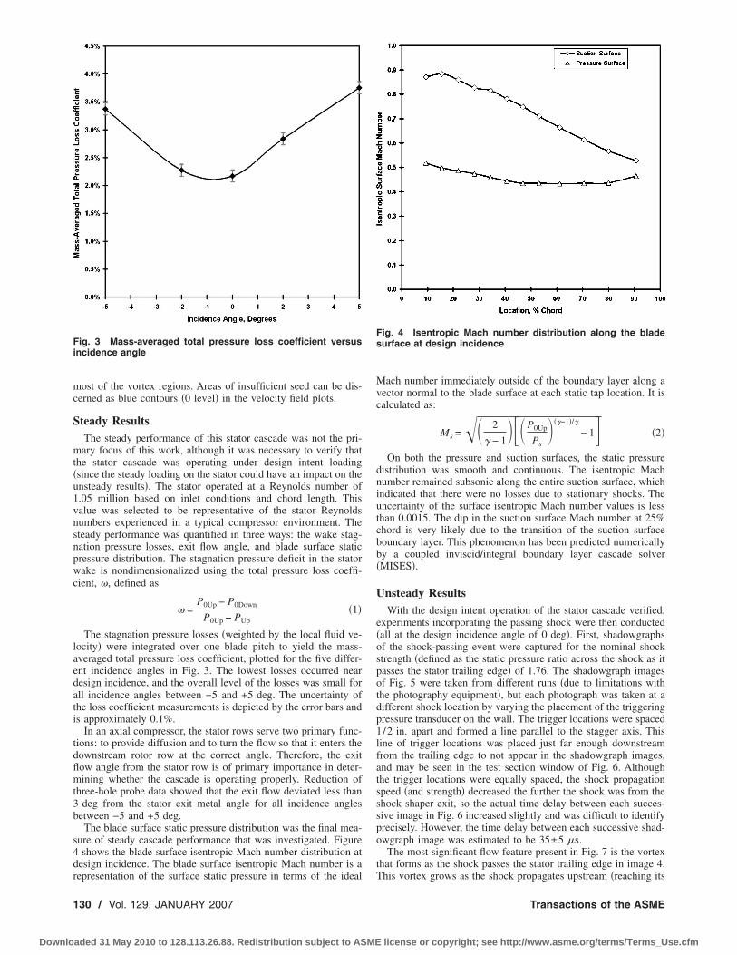
most of the vortex regions. Areas of insufficient seed can be dis-cerned as blue contours �0 level� in the velocity field plots.

Steady ResultsThe steady performance of this stator cascade was not the pri-

mary focus of this work, although it was necessary to verify thatthe stator cascade was operating under design intent loading�since the steady loading on the stator could have an impact on theunsteady results�. The stator operated at a Reynolds number of1.05 million based on inlet conditions and chord length. Thisvalue was selected to be representative of the stator Reynoldsnumbers experienced in a typical compressor environment. Thesteady performance was quantified in three ways: the wake stag-nation pressure losses, exit flow angle, and blade surface staticpressure distribution. The stagnation pressure deficit in the statorwake is nondimensionalized using the total pressure loss coeffi-cient, �, defined as

� =P0Up − P0Down

P0Up − PUp�1�

The stagnation pressure losses �weighted by the local fluid ve-locity� were integrated over one blade pitch to yield the mass-averaged total pressure loss coefficient, plotted for the five differ-ent incidence angles in Fig. 3. The lowest losses occurred neardesign incidence, and the overall level of the losses was small forall incidence angles between −5 and +5 deg. The uncertainty ofthe loss coefficient measurements is depicted by the error bars andis approximately 0.1%.

In an axial compressor, the stator rows serve two primary func-tions: to provide diffusion and to turn the flow so that it enters thedownstream rotor row at the correct angle. Therefore, the exitflow angle from the stator row is of primary importance in deter-mining whether the cascade is operating properly. Reduction ofthree-hole probe data showed that the exit flow deviated less than3 deg from the stator exit metal angle for all incidence anglesbetween −5 and +5 deg.

The blade surface static pressure distribution was the final mea-sure of steady cascade performance that was investigated. Figure4 shows the blade surface isentropic Mach number distribution atdesign incidence. The blade surface isentropic Mach number is arepresentation of the surface static pressure in terms of the ideal

Mach number immediately outside of the boundary layer along avector normal to the blade surface at each static tap location. It iscalculated as:

Ms =�� 2

� − 1��P0Up

Ps��−1�/�

− 1 �2�

On both the pressure and suction surfaces, the static pressuredistribution was smooth and continuous. The isentropic Machnumber remained subsonic along the entire suction surface, whichindicated that there were no losses due to stationary shocks. Theuncertainty of the surface isentropic Mach number values is lessthan 0.0015. The dip in the suction surface Mach number at 25%chord is very likely due to the transition of the suction surfaceboundary layer. This phenomenon has been predicted numericallyby a coupled inviscid/integral boundary layer cascade solver�MISES�.

Unsteady ResultsWith the design intent operation of the stator cascade verified,

experiments incorporating the passing shock were then conducted�all at the design incidence angle of 0 deg�. First, shadowgraphsof the shock-passing event were captured for the nominal shockstrength �defined as the static pressure ratio across the shock as itpasses the stator trailing edge� of 1.76. The shadowgraph imagesof Fig. 5 were taken from different runs �due to limitations withthe photography equipment�, but each photograph was taken at adifferent shock location by varying the placement of the triggeringpressure transducer on the wall. The trigger locations were spaced1/2 in. apart and formed a line parallel to the stagger axis. Thisline of trigger locations was placed just far enough downstreamfrom the trailing edge to not appear in the shadowgraph images,and may be seen in the test section window of Fig. 6. Althoughthe trigger locations were equally spaced, the shock propagationspeed �and strength� decreased the further the shock was from theshock shaper exit, so the actual time delay between each succes-sive image in Fig. 6 increased slightly and was difficult to identifyprecisely. However, the time delay between each successive shad-owgraph image was estimated to be 35±5 �s.

The most significant flow feature present in Fig. 7 is the vortexthat forms as the shock passes the stator trailing edge in image 4.This vortex grows as the shock propagates upstream �reaching its

Fig. 3 Mass-averaged total pressure loss coefficient versusincidence angle

Fig. 4 Isentropic Mach number distribution along the bladesurface at design incidence



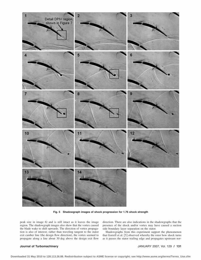
peak size in image 6� and is still intact as it leaves the imageregion. The shadowgraph images also show that the vortex causedthe blade wake to shift upwards. The direction of vortex propaga-tion is also of interest; rather than traveling tangent to the statorexit camber line �the design flow direction�, the vortex seemed topropagate along a line about 30 deg above the design exit flow

direction. There are also indications in the shadowgraphs that thepresence of the shock and/or vortex may have caused a suctionside boundary layer separation on the stator.

Shadowgraphs from this experiment support the phenomenonthat Gorrell et al. �5� observed whereby the rotor bow shock turnsas it passes the stator trailing edge and propagates upstream nor-

Fig. 5 Shadowgraph images of shock progression for 1.76 shock strength



mal to the blade surface. The shock has an angle relative to theblade suction surface of about 27 deg as it is passing the trailingedge in image 4, but has turned to be nearly 90 deg from the bladesurface by image 10. An explanation for the mechanism thatcauses this apparent turning of the shock is illustrated in Fig. 7.The figure shows the shock at time t and then diagrams the shockfront geometry as it advances from the stator trailing edge for time�t. The shock propagation velocity is shown as if it were constantin all directions �which was not the case in the experiment�, butthe concept remains valid. Although it is true that the shock isnormal to the blade surface in some shadowgraph images, it is

incorrect to conclude that this results in a higher static pressureratio or increased entropy rise relative to instances where theshock is oblique relative to the blade surface. In fact, the portionof the shock near the blade surface will be weaker than the ob-lique portion of the shock. If the shock were responsible for theobserved suction surface separation, a modification of the shockgeometry near the suction surface would result, a trend that wasnot evident in the shadowgraph images.

To provide more quantitative detail on the trailing edge vortexfrom Fig. 5, four DPIV velocity vector fields are presented in Fig.7. These DPIV images are centered on the stator trailing edge andare approximately 2.5 cm by 2.5 cm.

There are several important flow features present in Fig. 7:First, note the overall reduction in freestream velocity magnitudedue to the shock-passing event. This drop in velocity magnitude isdue to the superposition of the induced velocity field behind themoving shock with the unperturbed velocity field. The immediatenature of the velocity reduction across the moving shock may beseen in the DPIV image 5. The shock appears in the upper leftcorner of this image as a distinct velocity magnitude discontinuity.

DPIV also provides significantly more detail about the vortexflow field than the shadowgraphs, which merely show the vortexsize. It is clear from examining the velocity vectors in Fig. 7 thatthe vortex rotates in the opposite direction of the flow circulationaround the stator. The vortex is analogous to a starting vortex as itwas shed in response to the unsteady increase in circulation on thestator that was induced by the shock. The result of superimposingthe counter-clockwise rotating vortex with the freestream flow isincreased velocity on the lower side of the vortex but stagnatedflow on the upper side, thus leading to blockage. As the shadow-graphs also showed, the DPIV images illustrate the vortex grow-ing in size as it propagates downstream.

The trailing edge velocity field after the shock-passing eventwas also captured for three different shock strengths. While avortex clearly formed in each case, the size of the vortex provedto increase directly with shock strength. Figure 8 shows the trail-ing edge velocity vector fields for the three different shockstrengths at roughly the same time in the shock-passing cycle.

There are several significant trends visible in the images of Fig.8. Primarily, the magnitudes of the velocities in the vortex relativeto the freestream velocity increased with greater shock strength.Using the DPIV data, the size and strength of the vortex werededuced. Figure 9 shows the distribution of tangential velocity inthe vortex for the 1.76 shock strength case. The circulation can becomputed from the DPIV data as either the line integral of thevelocity at a given radius or the area integral of the vorticity. Bothmethods give similar results. Figure 9 also compares the measuredvortex tangential velocity with a Rankine vortex and a Newman�18� vortex. The Newman vortex is derived from laminar viscousassumptions and agrees well with the measurements. The multiplelines in Fig. 10 represent results computed using different as-

Fig. 6 Schematic of the shock turning phenomenon

Fig. 7 DPIV velocity fields of the trailing edge vortex createdby the moving shock „shock strength�1.76…, with the corre-sponding shadowgraph image number from Fig. 5

Fig. 8 Trailing edge velocity vector fields for three different shock strengths



sumed centers for the integration areas. The measured vortexstrength is relatively insensitive to precise identification of thevortex center.

The properties of the vortices generated by the three differentshock strengths investigated are presented in Table 2. The mea-sured vortex circulation is divided by the maximum angular ve-locity �� in the vortex to calculate a vortex radius R. The Machnumbers upstream and downstream relative to the shock are alsopresented. It is desirable to have a simple model that gives a guideto the induced vortex strength. The shock induces a velocity in theflowfield �dV�, and it is the component in the flowfield perpen-dicular to the trailing edge mean camber line �dVt� that drives thevortex formation. This perpendicular velocity, when multiplied by20% of the stator chord, gives a good correlation with the mea-

sured vortex circulation, as plotted in Fig. 11. The 20% chordvalue was arrived at as an arbitrary constant, but it is significantthat it is approximately representative of the length of the statorsubjected to the unsteady loading induced by the shock when thevortex detaches from the trailing edge of the stator as in image 5from Fig. 5.

Since flow velocity was the only parameter that was measuredin the vortex region, it would be difficult to calculate the stagna-tion pressure loss due to the shed vortices. Even if stagnationpressure measurements were available in the region, the resultswould be difficult to interpret since the shock itself added energyto the flowfield. Even an accurate means of directly measuring theunsteady cascade losses would be of limited value since this cas-cade test was not truly representative of the full repeating condi-tions that occur in an actual compressor. However, Crocco’s theo-rem gives a relationship that could be used to estimate the entropyin the vortex:

2� = 1/V��h0/�r − T � s/�r� �3�It is noted that vorticity requires gradients of entropy, stagna-

tion enthalpy, or both in the fluid. Analytical attempts to estimatethe entropy in the vortex have proved difficult, so loss estimateshave relied heavily on CFD simulation of the test configuration.Further loss will occur as the vortex core mixes out as it propa-gates downstream, and this can be estimated by assuming thevortex loses all its kinetic energy in the mixing process. The re-sultant losses in the vortex fluid may be high, but only affect therelatively small percentage of mass flow contained within the vor-tex core. A representative rotor passing frequency to this stator inan operating compressor would be 5500 Hz, and so each statorwould shed 5500 primary vortices per second. The mass flowcontained in these vortices compared to the mass flow in the free-stream would be relatively small, approximately 1% for the 1.76pressure ratio shock, so that the resultant mass-averaged loss inthe vortex is expected to be small. However, the effects of thevortex and its blockage, which can be considerable at some in-stances in time, on the downstream transonic rotor may also resultin a significant loss for an operating compressor stage.

The vortex in Fig. 11 travels approximately 6.5 mm in about100 �s, which corresponds to a propagation velocity of about65 m/s. This means the vortex travels downstream at roughly halfthe local freestream velocity, forcing the freestream flow to bypassthe slower-moving vortex. In this manner, the vortex acts as apassage blockage.

The best way to visualize the effects of the passage blockagedue to the vortex is to plot streamlines for the DPIV velocityfields. The unsteady nature of the trailing edge flowfield meansthat the calculated streamlines are instantaneous and do not rep-resent pathlines that a specific particle would take through theflow during the unsteady vortex-formation event. However, they

Fig. 9 DPIV measured vortex tangential velocity versus radiallocation within vortex and comparison to theory „shockstrength�1.76…

Fig. 10 Sensitivity of DPIV measured tangential velocity to er-ror in locating vortex center „shock strength�1.76…

Table 2 Vortex parameters

Shock strength

Parameter Units 1.42 1.76 2.10

Measured m2/s 1.27 1.64 2.60� rad/s 2432 2457 2984R mm 1.71 2.19 2.87�*R m/s 118 119 145M1

1.17 1.28 1.40M2

0.86 0.80 0.74dVt=dV* cos �� m/s 73.2 115.8 159.3Predicted

0 .2*dVt*Cm2/s 1.11 1.77 2.43

Fig. 11 Vortex circulation versus shock strength, measuredand predicted



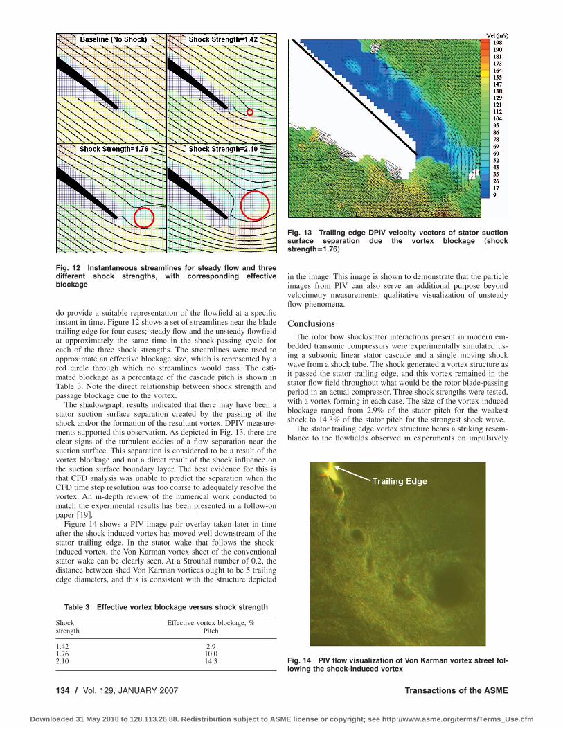
do provide a suitable representation of the flowfield at a specificinstant in time. Figure 12 shows a set of streamlines near the bladetrailing edge for four cases; steady flow and the unsteady flowfieldat approximately the same time in the shock-passing cycle foreach of the three shock strengths. The streamlines were used toapproximate an effective blockage size, which is represented by ared circle through which no streamlines would pass. The esti-mated blockage as a percentage of the cascade pitch is shown inTable 3. Note the direct relationship between shock strength andpassage blockage due to the vortex.

The shadowgraph results indicated that there may have been astator suction surface separation created by the passing of theshock and/or the formation of the resultant vortex. DPIV measure-ments supported this observation. As depicted in Fig. 13, there areclear signs of the turbulent eddies of a flow separation near thesuction surface. This separation is considered to be a result of thevortex blockage and not a direct result of the shock influence onthe suction surface boundary layer. The best evidence for this isthat CFD analysis was unable to predict the separation when theCFD time step resolution was too coarse to adequately resolve thevortex. An in-depth review of the numerical work conducted tomatch the experimental results has been presented in a follow-onpaper �19�.

Figure 14 shows a PIV image pair overlay taken later in timeafter the shock-induced vortex has moved well downstream of thestator trailing edge. In the stator wake that follows the shock-induced vortex, the Von Karman vortex sheet of the conventionalstator wake can be clearly seen. At a Strouhal number of 0.2, thedistance between shed Von Karman vortices ought to be 5 trailingedge diameters, and this is consistent with the structure depicted

in the image. This image is shown to demonstrate that the particleimages from PIV can also serve an additional purpose beyondvelocimetry measurements: qualitative visualization of unsteadyflow phenomena.

ConclusionsThe rotor bow shock/stator interactions present in modern em-

bedded transonic compressors were experimentally simulated us-ing a subsonic linear stator cascade and a single moving shockwave from a shock tube. The shock generated a vortex structure asit passed the stator trailing edge, and this vortex remained in thestator flow field throughout what would be the rotor blade-passingperiod in an actual compressor. Three shock strengths were tested,with a vortex forming in each case. The size of the vortex-inducedblockage ranged from 2.9% of the stator pitch for the weakestshock to 14.3% of the stator pitch for the strongest shock wave.

The stator trailing edge vortex structure bears a striking resem-blance to the flowfields observed in experiments on impulsively

Fig. 12 Instantaneous streamlines for steady flow and threedifferent shock strengths, with corresponding effectiveblockage

Table 3 Effective vortex blockage versus shock strength

Shockstrength

Effective vortex blockage, %Pitch

1.42 2.91.76 10.02.10 14.3

Fig. 13 Trailing edge DPIV velocity vectors of stator suctionsurface separation due the vortex blockage „shockstrength�1.76…

Fig. 14 PIV flow visualization of Von Karman vortex street fol-lowing the shock-induced vortex



started bodies �20–22�. This observation is the basis of the simplecorrelation presented that relates the vortex circulation to theshock-induced velocity and the stator chord length. An estimate ofthe loss incurred by the formation and mixing of the vortex struc-ture indicated that the loss potential in the vortex system itself wassmall. DPIV measurements also indicated the onset of suctionsurface boundary layer separation due to the vortex blockage insome cases, but the lack of resolution in this region hamperedattempts to quantify the losses due to this separation.

It is worth noting that the shock in the current work variessomewhat from the rotor leading edge shock structure in actualtransonic compressors. The leading edge shocks from actual tran-sonic rotors produce the same rapid rise in static pressure, but theyare followed by an expansion wave, which lowers the static pres-sure and turns the flow in order to maintain circumferential peri-odicity �23�. The rapid static pressure increase of the shock in thecurrent work is followed only by a gradual decay in static pres-sure. How a successive expansion wave would affect the vortexstructure is beyond the scope of this work, but poses an interestingtopic for future research and is discussed in the follow-on paper�19�.

AcknowledgmentThe authors would like to thank GE Aircraft Engines for pro-

viding the funding for this project and allowing the work to bepublished.

NomenclatureC � stator chord length

dV � shock-induced velocitydVt � shock-induced velocity component normal to

trailing edge camber lineh0 � stagnation enthalpy

M1 � relative Mach number upstream of shockM2 � relative Mach number downstream of shockMs � blade surface isentropic Mach number

P0Down � cascade downstream total pressureP0Up � cascade upstream total pressurePUp � cascade upstream static pressure

Ps � blade surface static pressurer � radial location within vortexR � vortex radiuss � entropyT � temperatureV � vortex circumferential velocity� � specific heat ratio

Measured � vortex circulation measured with DPIVPredicted � predicted vortex circulation

� � local total pressure loss coefficient� � vortex angular velocity

References�1� Denton, J. D., and Xu, L., 2002, “The Effects of Lean and Sweep on Transonic

Fan Performance,” ASME Paper No. GT-2002-30327.�2� Kerrebrock, J. L., 1981, “Flow in Transonic Compressors,” AIAA J., 19, pp.

4–19.�3� Lakshminarayana, B., 1996, Fluid Dynamics and Heat Transfer of Turboma-

chinery, Wiley, New York, pp. 99–107.�4� Prasad, A., 2003, “Evolution of Upstream Propagating Shock Waves From a

Transonic Compressor Rotor,” ASME J. Turbomach., 125, pp. 133–140.�5� Gorrell, S. E., Okiishi, T. H., and Copenhaver, W. W., 2003, “Stator-Rotor

Interactions in a Transonic Compressor—Part I: Effect of Blade-Row Spacingon Performance,” ASME J. Turbomach., 125, pp. 328–335.

�6� Gorrell, S. E., Okiishi, T. H., and Copenhaver, W. W., 2003, “Stator-RotorInteractions in a Transonic Compressor—Part II: Description of a Loss Pro-ducing Mechanism,” ASME J. Turbomach., 125, pp. 336–345.

�7� Estevadeordal, J., Gogineni, S., Goss, L., Copenhaver, W., and Gorrell, S.,2002, “Study of Wake-Blade Interactions in a Transonic Compressor UsingFlow Visualization and DPIV,” ASME J. Fluids Eng., 124, pp. 166–175.

�8� Sanders, A. J., Papalia, J., and Fleeter, S., 2002, “A PIV Investigation ofRotor-IGV Interactions in a Transonic Compressor,” J. Propul. Power, 18�5�,pp. 969–977.

�9� Zachcial, A., and Nurnberger, D., 2000, “A Numerical Study on the Influenceof Vane-Blade Spacing on a Compressor Stage at Sub and Transonic OperatingConditions,” ASME Paper No. GT2003-38020.

�10� Douglas, J. W., 2001, “Effects of Free Stream Turbulence on CompressorCascade Performance,” M.S. thesis, Virginia Polytechnic Institute and StateUniversity, Blacksburg, VA.

�11� Anderson, J. D., 1982, Modern Compressible Flow, McGraw-Hill, New York,pp. 202–203.

�12� Doughty, R. L., 1994, “Effects of Multiple Incident Shock Waves on the Flowin a Transonic Turbine Cascade,” Ph.D. dissertation, Virginia Polytechnic In-stitute and State University, Blacksburg, VA.

�13� Chester, W., 1960, “The Propagation of Shock Waves Along Ducts of VaryingCross Section,” Adv. Appl. Mech., VI, pp. 119–152.

�14� Nettleton, M. A., 1973, “Shock Attenuation in a Gradual Area Expansion,” J.Fluid Mech., 60, pp. 209–223.

�15� Sloan, S. A., and Nettleton, M. A., 1975, “A Model for the Axial Decay of aShock Wave in a Large Abrupt Area Change,” J. Fluid Mech., 71, pp. 769–785.

�16� Melling, A., 1997, “Tracer Particles and Seeding for Particle Image Velocim-etry,” Meas. Sci. Technol., 8, pp. 1406–1416.

�17� Westerweel, J., 1997, “Fundamentals of Digital Particle Image Velocimetry,”Meas. Sci. Technol., 8, pp. 1379–1392.

�18� Newman, B. G., 1958, “Flow in a Viscous Trailing Vortex,” Aeronaut. Q.,10�2�, pp. 149–162.

�19� van de Wall, A., Breeze-Stringfellow, A., and Dailey, L., 2006, “Computa-tional Investigation of Unsteady Flow Mechanisms in Compressors With Em-bedded Supersonic Rotors,” ASME Paper No. GT2006-90633.

�20� Pullin, D. I., and Perry, A. E., 1980, “Some Flow Visualization Experimentson the Starting Vortex,” J. Fluid Mech., 97�2�, pp. 239–255.

�21� Auerbach, D., 1987, “Experiments on the Trajectory and Circulation of theStarting Vortex,” J. Fluid Mech., 183, pp. 185–198.

�22� Lian, Q. X., and Huang, Z., 1989, “Starting Flow and Structures of the StartingVortex Behind Bluff Bodies with Sharp Edges,” Exp. Fluids, 8, pp. 95–103.

�23� Kerrebrock, J. L., 1977, Aircraft Engines and Gas Turbines, MIT, Cambridge,MA, pp. 135–138.



Elisabet Syverud

Lars E. Bakken

Department of Energy and Process Engineering,NTNU,

Norwegian University of Science and Technology,Trondheim, Norway

Online Water Wash Testsof GE J85-13This paper reports the results of a series of online water wash tests of a GE J85-13 jetengine at the test facilities of the Royal Norwegian Air Force. The engine performancewas deteriorated by injecting atomized saltwater at the engine inlet. The engine was thenonline washed with water injected at three different droplet sizes (25, 75, and 200 �m)and at water-to-air ratios ranging from 0.4% to 3% by mass. Engine performance wasmeasured using standard on-engine instrumentation. Extra temperature and pressuresensors in the compressor section provided additional information of the propagation ofdeposits in the aft stages. The measurements were supported by visual observations. Theoverall engine performance improved rapidly with online wash. The buildup of depositsin the aft stages was influenced both by the droplet size and the water-to-air ratio. Thewater-to-air ratio was the most important parameter to achieve effective onlinewashing. �DOI: 10.1115/1.2372768�

Keywords: compressor cleaning, axial compressor, stage characteristics, GE J85-13

IntroductionOnline water washing has become increasingly important with

operators of industrial gas turbines due to the potential for reduceddegradation rate and increased operating intervals. Successful on-line washing requires close attention to the gas turbine flow pathgeometry, the operating profile, and the nature of the airbornefouling at the compressor inlet �after filtration�.

Several manufacturers offer online washing equipment andmany patents exist relating to gas turbine water wash. There iscurrently no consensus on a recommended method for effectiveonline water washing. System properties like droplet size, dropletvelocity, and fluid injection rate vary from one system to another.This makes it difficult for operators to select the best online waterwash system for their application. Two recent publications give ahistorical review of online washing systems and a classification ofavailable systems �1,2�.

Today’s online washing equipment for aeroderivative enginescan be categorized in two main pressure ranges: Fluid pressuresup to 10 bar are considered low pressure systems, while high pres-sure systems have fluid pressures above 50 bar. The atomizeddroplets produced by high pressure systems have a droplet diam-eter typically less than 150 �m and resemble the water occurringnaturally in clouds and fog. Low pressure systems will havelarger, drizzle-like droplets with diameter ranging from100 to 500 �m and larger. Low pressure systems with air assistednozzles will generate smaller droplet sizes, resembling the drop-lets of the high pressure systems. Large droplets may cause bladeerosion in the compressor �2–5�.

The fluid injection rate �water-to-air ratio� has an impact on theinternal surface wetting of the compressor. Due to possible controlinstabilities, flame-out, or blade erosion the water-to-air ratio hasgenerally been kept low. A typical online washing system foraeroderivative engines has fluid injection in the range from 0.2%to 0.8% �mass based� �2–5�.

The flow field within an axial compressor subject to water in-jection is complex to predict due to the two-phase nature of theflow. The motion of water droplets inside axial compressors hasbeen studied for droplets smaller than 70 �m �6�. Experimental

work on a six stage axial compressor gives data for droplets of 90and 600 �m and at water injection rates up to 15% �by mass� �7�.Several papers offer theoretical approaches to wet compression�8–10�. These studies are related to tiny droplets, less than 15 �m,with no velocity slip between the droplet and air. A study of theeffects on gas turbines of naturally occurring water in the atmo-sphere gives additional insight into the operating limitations ofgas turbine engines �11�.

To understand and reveal the mechanisms related to online wa-ter washing, a systematic test campaign was performed on a GEJ85-13 jet engine. The engine performance was deteriorated byinjecting atomized saltwater at the engine inlet and the engineperformance was restored using online water washing. The waterwas injected at three different droplet sizes �25, 75, and 200 �m�at water-to-air ratios from 0.4% to 3% by mass. The cleaningeffectiveness was measured in terms of improved engine perfor-mance using standard on-engine instrumentation. Further, extratemperature and pressure sensors installed in the compressor sec-tion provided additional information on the propagation of thedeposits into the engine. The measurements were supported byvisual observations through the borescope and by laboratoryanalysis of the stator vane deposits. The results of the axial com-pressor deterioration are reported in a different publication �12�,and that paper should be seen in context with the present work.The test facilities, the GE J85-13 engine and its initial condition,the engine instrumentation, and the deterioration method is de-scribed in the present paper only when required for completeness.

Test Facilities and Engine DescriptionEngine testing was carried out at the Royal Norwegian Air

Force �RNoAF� test facilities at Kjeller, Norway.The General Electric J85-13 engine is a compact, light weight,

single-spool turbojet engine. It has an eight-stage axial-flow com-pressor with bleed-off valves, adjustable inlet guide vanes and avariable exhaust nozzle. The compressor pressure ratio is 6.5:1.The variable geometry is controlled by the throttle angle, but thetiming is ambient temperature biased. At International Organiza-tion for Standardization �ISO� conditions, inlet guide vanes �IGV�will be at maximum deflection and bleed-off-valves will be fullyopen below �81% corrected speed and fully closed at �96%corrected speed. At ambient temperatures above ISO conditions,the bleed-off-valves will close at lower speed settings. The nozzleis controlled by the throttle when the engine is running below theexhaust temperature limit. When the maximum exhaust tempera-




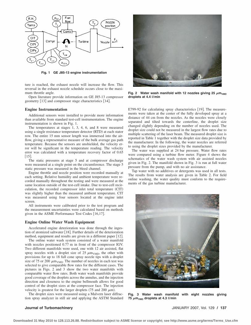
ture is reached, the exhaust nozzle will increase the flow. Thisreversal in the exhaust nozzle schedule occurs close to the maxi-mum throttle angle.

Open literature provide information on GE J85-13 compressorgeometry �13� and compressor stage characteristics �14�.

Engine InstrumentationAdditional sensors were installed to provide more information

than available from standard test-cell instrumentation. The engineinstrumentation is shown in Fig. 1.

The temperatures at stages 1, 3, 4, 6, and 8 were measuredusing a single resistance temperature detector �RTD� at each statorrow. The entire 15 mm sensor length was immersed into the air-flow, giving a representative measure of the bulk average gas pathtemperature. Because the sensors are unshielded, the velocity er-ror will be significant in the temperature reading. The velocityerror was calculated with a temperature recovery factor of 0.65�15�.

The static pressures at stage 5 and at compressor dischargewere measured at a single point on the circumference. The stage 5static pressure was measured in the bleed channel.

Engine throttle and nozzle position were recorded manually ateach setting. Relative humidity and ambient temperature were re-corded manually throughout the testing and were measured at thesame location outside of the test-cell intake. Due to test-cell recir-culation, the recorded compressor inlet total temperature �CIT�was slightly higher than the measured ambient temperature. CITwas measured using four sensors located at the engine inletscreen.

All instruments were calibrated prior to the test program andthe measurement uncertainties were calculated based on methodsgiven in the ASME Performance Test Codes �16,17�.

Engine Online Water Wash EquipmentAccelerated engine deterioration was done through the inges-

tion of atomized saltwater �18�. Further details of the deteriorationmethod, equipment and results are given in a different paper �12�.

The online water wash system consisted of a water manifoldwith nozzles positioned 0.77 m in front of the compressor IGV.Two different manifolds were used, one with 12 air assisted, flatspray nozzles with a droplet size of 25 �mVMD, the other withprovisions for up to 18 full cone spray nozzle tips with a dropletsize of 75 or 200 �mVMD. The number of nozzles in each test wasselected to give comparable flow rates for the different cases. Thepictures in Figs. 2 and 3 show the two water manifolds withcomparable water flow rates. Both water wash manifolds providegood coverage of the droplets across the annulus, and the injectiondirection and closeness to the engine bellmouth allows for goodcontrol of the droplet sizes at the compressor face. The injectionvelocity is greatest for the larger droplets �75 and 200 �m�.

The droplet sizes were measured using a Malvern laser diffrac-tion spray analyzer in still air and applying the ASTM Standard

E799-92 for calculating spray characteristics �19�. The measure-ments were taken at the center of the fully developed spray at adistance of 44 cm from the nozzles. As the nozzles were closelyseparated and tilted towards the centerline, the droplet sizechanged slightly depending on the number of nozzles used. Thedroplet size could not be measured in the largest flow rates due tomultiple scattering of the laser beam. The measured droplet size isreported in Table 1 together with the droplet size data provided bythe manufacturer. In the following, the water nozzles are referredto using the droplet sizes provided by the manufacturer.

The water was supplied at 24 bar pressure. Water flow rateswere compared using a turbine flow meter. Figure 4 shows theschematics of the water wash system with air assisted nozzlesgiven in Fig. 2. The manifold shown in Fig. 3 is run at full waterpressure from the pump, and with no air assistance.

Tap water with no additives or detergents was used in all tests.The results from water analysis are given in Table 2. For fieldonline washing, the water quality must conform to the require-ments of the gas turbine manufacturer.

Fig. 1 GE J85-13 engine instrumentation

Fig. 2 Water wash manifold with 12 nozzles giving 25 �mVMDdroplets at 4.4 l /min

Fig. 3 Water wash manifold with eight nozzles giving75 �mVMD droplets at 4.3 l /min



Test ProcedureThe engine base lines were established for steady-state opera-

tion at 12 operating points from 60% corrected speed to full load.Prior to establishing each base line, the engine was run for 5 minat full load. Engine speed was then reduced to idle before beingincreased to the initial throttle setting. At each throttle setting, theengine was allowed to stabilize for 1 min before reading 60 datapoints. To prevent impact of hysteresis from the instrument orcontrol system, all throttle settings were established at increasingengine speeds. Engine base lines were recorded prior to degrada-tion, after salt degradation, and after each online water wash.

All salt degradation trials and online water wash tests were runat 10 deg throttle angle �equivalent to 97.5% engine shaft speed�at constant nozzle position and with closed bleed-off-valves andfully open IGV.

To completely clean the compressor of salt deposits, a 5 minonline water wash was done at engine speeds varying from fullspeed to idle for two complete cycles using 17.6 l of water perminute �droplet size of 200 �m�.

Seven online water wash tests were completed. The test matrixis given in Table 1. Engine performance was measured after 30,60, 90 s, 4 min, and 10 min online water wash.

ResultsThe engine performance deterioration and restoration was ana-

lyzed through changes in the intake depression and in the com-pressor stage work coefficient. Intake depression is defined as thedeviation between the total and static pressure at engine inlet.Detailed background on the stage performance calculations isgiven in a different publication �12�, and will not be repeated here,since the only difference is the blockage factor which is set to 1.0for all cases presented in this paper.

The presented test data are limited to engine operation above95% engine shaft speed where the engine bleed-off valves wereclosed and the IGV were fully open.

The test data are compared to the stage work coefficient �14�.Those data are based on constant values for cp �1005 J /kg K� and� �1.4�, while here the gas properties are dependent on gas tem-perature and humidity. The difference will be largest in the aftstages where the gas temperatures are at the highest. Nonetheless,the published data give a good indication of the GE J85-13 stageperformance for a large range of flow coefficients.

Water-to-Air Ratio. The GE J85-13 was operated without sta-bility or structural problems at water injection rates of 40 l /min atall speeds from 70% to full speed. This represents mass basedwater-to-air ratios above 3% at full speed and 7% at 70% speed.However, these very high water-to-air ratios may cause excessiveblade loads and potential erosion damage and are not recom-mended for online water washing.

Figure 5 shows the change in intake depression as a function ofcorrected engine shaft speed for three different water-to-air ratioswith 200 �m droplet size and 1 min water injection time.

Figures 6 and 7 show the change in stage work coefficient forthe same cases as given in Fig. 5. Stage four performance is notrestored with the smallest water-to-air ratio of 0.43%. The remain-ing salt deposits reduce the effective flow area and cause a reduc-tion in the stage six flow coefficient. With a 3% water-to-air ratiosixth stage performance is restored.

The tests clearly document the impact of increased water-to-airratio on the compressor performance recovery. At low water-to-airratios, performance recovery is limited.

Water Injection Time. Increasing the water injection time ofonline water wash is expected to improve performance recoverywhen the engine is fouled with water soluble components such assalt �1�.

Figure 8 compares the change in intake depression for three

Table 2 Analysis of water used for online water wash

Parameter Value

Total matter �1 mg/ lpH 7.52Sodium 2.1 ppm by weightPotassium 0.63 ppm by weightChloride 1.7 ppm by weight

Fig. 4 Water wash system schematics „air assisted nozzles…Fig. 5 Intake depression recovery after 60 s water wash with200 �m droplets

Table 1 Test matrix

Testnumber

Droplet size ��mVMD�

Water flow rate�l/min�

Water-to-air ratio�%�

Frommanufacturer Measured

1 200 — 30.9 3.02 200 — 17.6 1.73 200 131 8.8 0.874 200 139 4.4 0.435 75 83 9.1 0.896 75 93 4.3 0.427 25 39 4.4 0.43



different cases with 200 �m droplet size. The total water injectedin the 4 min water wash at 0.43% water-to-air ratio is equivalentto the total water injected during the 1 min water wash at 1.7%water-to-air ratio. The 0.43% 1 min water wash case is includedfor reference. The impact on stage four and six work coefficientsare given in Figs. 9 and 10, respectively.

Although an equivalent mass of water is used in the 1.7% 1 minwash and the 0.43% 4 min wash, the increased water injectiontime at lower flow rate fails to recover engine performance. Withthe low water-to-air ratio of 0.43%, the water seems to evaporatein stage four and the expected benefit from increased soaking timeis therefore not apparent.

The tests show that water injection time is only an issue in thefront stages where the wash fluid is not evaporated. For aft stageperformance recovery, it is better to inject the water in a shortertime, hence, at a higher water-to-air ratio.

Droplet Size. Droplet size is considered important for perfor-mance recovery in the aft compressor stages. Water flow path,surface wetting, evaporation rate, and erosion are all affected by

the droplet size.Figures 11–13 compare the intake depression restoration and

the stage four and six work coefficient recovery after 1 min onlinewater wash at a water-to-air ratio of 0.4% and with various dropletsizes.

The 75 �m droplets are the most effective in recovering theoverall engine performance, and in cleaning the fourth stage; how-ever, the smaller droplets seem to redeposit the fouling in the sixthstage and cause increased sixth stage deterioration. The 25 �mdroplets cause heavy deposits in the sixth stage and are the leasteffective in restoring the overall engine performance.

The tests show that small droplets increase the fouling in the aftstages.

Salt Distribution After Water Wash. Further evidence of themovement of salt from the front stages to the aft stator vanes isgiven in Fig. 14. The figure compares the salt deposits on thestator vanes after degradation to the salt distribution after a 1 minwater wash with 75 �m droplets and 0.42% water-to-air ratio. Thesalt deposits were measured as chlorine content and converted to

Fig. 6 Stage 4 work coefficient after 60 s water wash with200 �m droplets

Fig. 7 Stage 6 work coefficient after 1 min water wash with200 �m droplets

Fig. 8 Intake depression recovery at different water injectiontimes with 200 �m droplets

Fig. 9 Stage 4 work coefficient after water wash with 200 �mdroplets at different water injection times



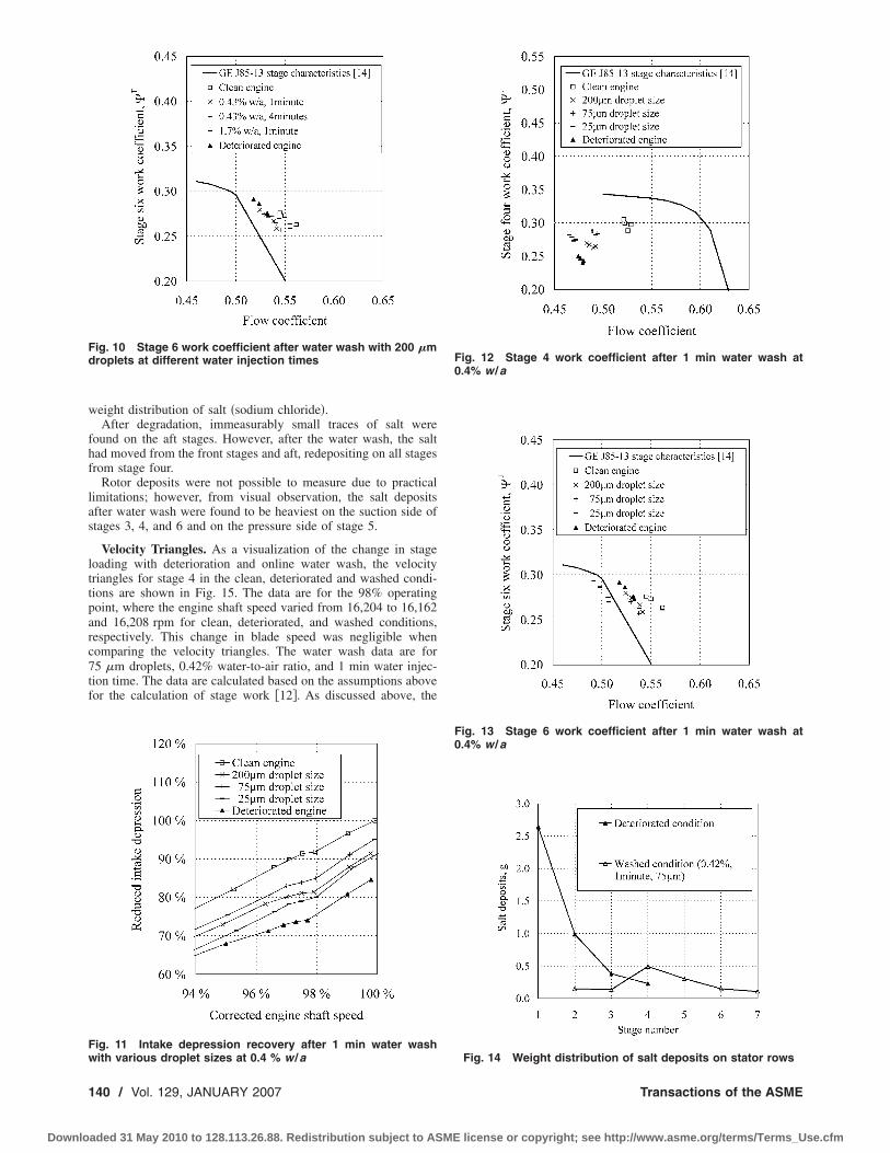
weight distribution of salt �sodium chloride�.After degradation, immeasurably small traces of salt were

found on the aft stages. However, after the water wash, the salthad moved from the front stages and aft, redepositing on all stagesfrom stage four.

Rotor deposits were not possible to measure due to practicallimitations; however, from visual observation, the salt depositsafter water wash were found to be heaviest on the suction side ofstages 3, 4, and 6 and on the pressure side of stage 5.

Velocity Triangles. As a visualization of the change in stageloading with deterioration and online water wash, the velocitytriangles for stage 4 in the clean, deteriorated and washed condi-tions are shown in Fig. 15. The data are for the 98% operatingpoint, where the engine shaft speed varied from 16,204 to 16,162and 16,208 rpm for clean, deteriorated, and washed conditions,respectively. This change in blade speed was negligible whencomparing the velocity triangles. The water wash data are for75 �m droplets, 0.42% water-to-air ratio, and 1 min water injec-tion time. The data are calculated based on the assumptions abovefor the calculation of stage work �12�. As discussed above, the

Fig. 12 Stage 4 work coefficient after 1 min water wash at0.4% w /a

Fig. 13 Stage 6 work coefficient after 1 min water wash at0.4% w /a

Fig. 14 Weight distribution of salt deposits on stator rows

Fig. 10 Stage 6 work coefficient after water wash with 200 �mdroplets at different water injection times

Fig. 11 Intake depression recovery after 1 min water washwith various droplet sizes at 0.4 % w /a



deviation angles are assumed constant for the clean and deterio-rated cases. Equations for the calculations of velocity triangles aregiven in the Appendix.

The velocity triangles show that the deterioration causes a re-duction in the flow coefficient and a change in the stage workcoefficient.

ConclusionsOnline water washing has become increasingly important with

operators of industrial gas turbines due to the potential for reduceddegradation rate, increased operating intervals, and high overallperformance.

To reveal the compressor performance deterioration and resto-ration mechanisms, an in-depth test campaign has been performedon a GE J85-13 engine. Based on test results and performanceanalyses the main mechanisms are:

• High water flow rate is the most significant parameter foreffective online water wash.

• Low flow rates cause redeposition of the fouling in the aftstages.

• Increased water injection time cannot compensate for lowflow rates.

• Smaller droplets increase the fouling in the aft stages.

For effective water washing of the entire compressor section,the recommended water-to-air ratio is between 0.8% to 2%. Drop-let diameters up to 200 �m have been tested. The maximum drop-let size and water-to-air ratio should be determined with closeattention to blade erosion and other long term mechanical andstructural problems.

The present achievements will be followed by field tests on aRolls-Royce RB 211 in an offshore application.

AcknowledgmentThe project has been supported by Statoil ASA, Dresser-Rand

Norwegian Operations, and the Royal Norwegian Navy. TheRoyal Norwegian Air Force is acknowledged for allowing accessto their test facilities and for allowing the authors to borrow a GEJ85-13 for test purposes. Without the help of Hans K. Henriksen,a retired test-cell operator of the RNoAF, this project would neverhave come to fruition.

NomenclatureA � flow area �m2�cp � specific heat at constant pressure �kJ/kgK�C � absolute air velocity �m/s�

CIT � compressor inlet temperature �K�CIP � compressor inlet pressure �kPa�GE � General Electric

IGV � inlet guide vanes

ISO � International Organization forStandardization1

m � mass flow rate �kg/s�N � shaft speed �rpm�

NASA � National Aeronautics and SpaceAdministration

p � pressure �kPa�r � blade radius �m�R � gas constant �kJ/kg K�

R.H. � relative humidity �%�RNoAF � Royal Norwegian Air Force

RTD � resistance temperature detectorT � temperature �K�U � blade velocity �m/s�V � relative air velocity �m/s�

w /a � water-to-air ratio �kg H2O/kg air�

Greek Symbols� � absolute air angle �deg�� relative air angle �deg�� air density �kg/m3�� ratio of specific heats

T=cpTt /Utip2 � stage work coefficient

�=Ca /Utip � flow coefficient

Subscriptsa � axial velocity component

amb � ambient conditionmix � mixture �humid air�

s � static conditiont � total condition

tip � tipVMD � volume median diameter

w � tangential velocity component2.1,2.2,…,2.7 � compressor stage 1,2,…, to stage 7

3 � compressor discharge5 � turbine discharge

Appendix: Equations for Calculations of Velocity Dia-gram

Data for the velocity diagram are readily available from theiterative calculation of stage performance �12�.

Consider a stage where the rotor inlet, rotor outlet, and statoroutlet are designated as stations 1, 2, and 3, respectively.

1 The absolute air velocities and the blade velocity are knownfrom the stage performance calculations at the rotor inlet:Ca1, C1, Cw1, U1

2 The relative velocity at rotor inlet is calculated from

Vw1 = U1 − Cw1, V1 = �Vw12 + Ca1

2

3 The tangential blade velocity at rotor outlet is given by

U2 = 2�r2N

60

4 The tangential component of the absolute velocity at rotoroutlet is given by the change in work input

Cw2 =cp1�Tt2 − Tt1� + Cw1U1

U2

5 Consequently, the absolute velocity at rotor outlet is

C2 = �Cw22 + Ca2

2

6 And the relative velocity at rotor outlet is given by

1ISO reference conditions assume an ambient temperature of 288.15 K, a baro-metric pressure of 101.325 kPa, and a relative humidity of 60%.

Fig. 15 Stage 4 velocity triangles at 98% shaft speed



Vw2 = U2 − Cw2, V2 = �Vw22 + Ca2

2

7. Knowing the velocity vectors, the absolute and relative airangles at rotor inlet and outlet are given from geometry

� = arctan�Cw

Ca�, � = arctan�Vw

Ca�

8. The stator exit velocity is found from assuming zero devia-tion in the stator blade exit angle: Ca3= m /�3A3, C3=Ca3 /cos��3�.

References�1� Stalder, J.-P., 2001, “Gas Turbine Compressor Washing State of the Art: Field

Experiences,” ASME J. Eng. Gas Turbines Power, 123, pp. 363–370.�2� Mund, F., and Pilidis, P., 2004, “A Review of Online Washing Systems,”

ASME Paper No. GT2004–53224.�3� Asplund, P., 1997, “Gas Turbine Cleaning Upgrade �Compressor Wash�,”

ASME Paper No. 97-AA-135.�4� Asplund, P., and Hjerpe, C. J., 2004, “A Method for Cleaning a Stationary Gas

Turbine Unit During Operation,” World Patent No. WO2004/055334.�5� Faddegon, C. J., 1999, “Effective Compressor Cleaning as a Result of Scien-

tific Testing and Field Experience,” FP Turbomachinery Consultants GmbH,Spinzalaan 177-C, 2273 XG Voorburg, The Netherlands.

�6� Marchik, A., 1965, “Motion of Condensed Phase in the Blade Passages of anAxial Gas Turbine Stage,” Teploenergetika, pp. 51–57.

�7� Tsuchiya, T., and Murthy, S. N. B., 1982, “Water Ingestion Into Jet EngineAxial Compressors,” AIAA Paper No. 82–0196.

�8� Horlock, J. H., 2001, “Compressor Performance With Water Injection,” Pro-ceedings of ASME Turbo Expo 2001, June 4–7, New Orleans, LA.

�9� Young, J. B., 1995, “The Fundamental Equations of Gas-Droplet MultiphaseFlow,” Int. J. Multiphase Flow, 21�2�, pp. 175–191.

�10� Meacock, A. J., and White, A. J., 2006, “The Effect of Water Injection onMultispool Gas Turbine Behavior,” ASME Paper No. GT2004–53320.

�11� Garwood, K. R., 1995, “Recommended Practices for the Assessment of theEffects of Atmospheric Water Ingestion on the Performance and Operability ofGas Turbine Engines,” AGARD Advisory Report AGARD AR-332.

�12� Syverud, E., Brekke, O., and Bakken, L. E., 2007, “Axial Compressor Dete-rioration Caused by Saltwater Ingestion,” ASME J. Turbomach., 129�1�, pp.119–126.

�13� Tesch W. A., and Steenken, W. G., 1976, “Blade Row Dynamic Digital Com-pressor Program Volume 1 J85 Clean Inlet Flow and Parallel CompressorModels,” NASA CR-134978.

�14� Milner, E. J., and Wenzel, L. M., 1975, “Performance of a J85–13 CompressorWith Clean and Distorted Inlet Flow,” NASA TM X-3304.

�15� Saravanamuttoo, H. I. H., ed., 1990, “Recommended Practices for Measure-ment of Gas Path Pressures and Temperatures for Performance Assessment ofAircraft Turbine Engines and Components,” AGARD Advisory ReportAGARD AR-245.

�16� ASME, 1997, Performance Test Code on Gas Turbines, ASME PTC-22,ASME, New York.

�17� ASME, 1998, Test Uncertainty, ASME PTC-19.1, ASME, New York.�18� Caguiat, D. E., Zipkin, D. M., and Patterson, J. S., 2002, “Compressor Fouling

Testing on Rolls Royce/Allison 501-K17 and General Electric LM 2500 GasTurbine Engines,” ASME Paper No. GT2002–30262.

�19� ASTM Standard E 799–92, 1992, “Standard Practice for Determining DataCriteria and Processing for Liquid Drop Size Analysis,” ASTM International,West Conshohocken, PA.



E. P. Petrov

D. J. Ewins

Mechanical Engineering Department,Centre of Vibration Engineering,

Imperial College London,South Kensington Campus,

London SW7 2AZ, UK

Advanced Modeling ofUnderplatform FrictionDampers for Analysisof Bladed Disk VibrationAdvanced structural dynamic models for both wedge and split underplatform dampershave been developed. The new damper models take into account inertia forces and theeffects of normal load variation on stick-slip transitions at the contact interfaces. Thedamper models are formulated for the general case of multiharmonic forced responseanalysis. An approach for using the new damper models in the dynamic analysis oflarge-scale finite element models of bladed disks is proposed and realized. Numericalinvestigations of bladed disks are performed to demonstrate the capabilities of the newmodels and an analysis of the influence of the damper parameters on the forced responseof bladed disks is made. �DOI: 10.1115/1.2372775�

IntroductionDue to the high density of natural frequencies of realistic

bladed disks and of the broad spectrum of aerodynamic excitationforces, the complete avoidance of all resonance regimes is notgenerally possible. Thus, the use of special devices that dissipatevibration energy and, hence, reduce the resonance amplitudes toacceptable levels is usually essential. One of the most effectivetypes of damping device is the underplatform friction damper�UPD� that is generally a small piece of metal which frequentlyhas a wedge-like or other shape, and which is usually locatedunderneath the blade platforms. Damping of the blade vibration isachieved by friction forces acting at the contact interfaces be-tween blades and dampers. Dissipation of vibration energy intothermal starts when blade displacements reach a certain level.This level, and the effectiveness of reducing forced response lev-els by using underplatform dampers, is highly dependent on thechoice of the damper parameters. Optimal selection of these pa-rameters can only be made efficiently when accurate modelingand analysis tools are available to provide capabilities for reliableprediction of the forced response levels for bladed discs with thedampers.

There is more than 30 years of history of development of mod-els for dynamic analysis of bladed disks with friction dampers.The simplest model which was applied initially for analysis of ablade-damper system was a classical single-degree-of-freedom�SDOF� oscillator with Coulomb friction. The first engineeringfriction damper models were investigated and experimentally vali-dated in Refs. �1,2�. These models, while still applied to the SDOFblade model, were essentially spring-slider models, which in-cluded not only friction but also the flexibility effect introducedby the damper. Development of these models for cases of multi-harmonic forced response is considered in Refs. �3,4�. Multibodymodel for a two-bladed system with a damper was proposed inRef. �5� where a 2DOF model was used for each of two bladesand 3DOF model for a friction damper with two contact inter-faces. Coulomb-style friction damper models are also applied formultiharmonic forced response analysis in Refs. �6,7�.

In real conditions underplatform friction dampers have at least

two interfaces at which they interact with adjacent blades. In orderto obtain a more accurate prediction of the forced response inconjunction with multidegree-of-freedom blade models, several“kinematic” models were developed in Refs. �8–11�. These mod-els are based on some kinematic hypothesis about the relativemotion of a wedge-shape damper and blade platform. The damperand blade platforms are considered as some kind of mechanismobeying this kinematic hypothesis and hence the damper’s dynam-ics are ignored and inertia forces are neglected. As a result, thefriction forces are expressed in these models ultimately throughmotion of the blade platforms. In order to describe microslip at thecontact interfaces two approaches were explored: �i� representa-tion of friction contact by an array of spring-slider elements withdifferent parameters �see Ref. �8�� and �ii� use of an analyticalsolution for friction forces between a bar and a foundation sup-porting this bar �see Refs. �9,10��. Underplatform dampers ofsemi-cylindrical and wedge shapes were studied in Ref. �12� withaccounting for damper inertia forces due to rigid body motion.The idea of using two-piece dampers, so-called “split dampers”�SD� for increase of energy dissipation and first kinematic-hypothesis-based models for split dampers were proposed in Ref.�13�.

Friction contact modeling capabilities and multiharmonicanalysis code developed in Ref. �14� were applied in Ref. �15� toexplore possibilities of forced response analysis of flexible finiteelement damper models using a two-blade system.

However, all engineering damper models require informationabout friction coefficient and damper stiffness to be supplied. Theproblem of determining contact stiffness for dampers and its rolein forced response prediction was studied in Ref. �16� using de-tailed finite element models for contact areas.

Damper models need to be further improved to allow moreaccurate and reliable quantitative predictions of forced response.Among the phenomena which are still not included in existingmodels are the effects of variation of the normal load on stick-sliptransitions at damper contact interfaces �see some of these effectsin Ref. �17��. Moreover, in the majority of damper models existedto date only monoharmonic forced response is considered. Thereare dampers of such designs that still do not have fully consistent,not-contradictory models. One of those damper designs is adamper consisting from two or more separate parts.

In this paper, new models for underplatform dampers of differ-ent designs are developed. The models are aimed at multihar-monic forced response analysis of large-scale realistic finite ele-

Contributed by the International Gas Turbine Institute �IGTI� of ASME for pub-lication in the JOURNAL OF TURBOMACHINERY. Manuscript received October 1, 2005;final manuscript received February 1, 2006. IGTI Review Chair: R. S. Abhari. Paperpresented at the ASME Turbo Expo 2006, Barcelona, Spain, May 8–11, 2006, PaperNo. GT2006-90146.



ment models of bladed disks with underplatform dampers. Modelsfor dampers consisting a single piece of metal, so-called “cottageroof damper” �CRDs� and for split dampers �SD� are developed.CRDs and SDs of symmetric and asymmetric geometry shapes areconsidered. The dynamic damper models are developed whichtake into account here damper inertia properties. The flexibility ofthe underplatform dampers, together with the elasticity or stiffnessproperties of a layer of microasperities which is due to the rough-ness of contact surfaces is considered. Forces at contact interfacesare described by advanced friction contact models previously de-veloped by the authors in Refs. �17,18�. The friction models in-clude all the effects of variation of normal load on friction forces,including its influence on slip-stick transitions, and allow for tem-porary separation of the contact surfaces. Numerical investiga-tions of bladed disks are performed to demonstrate and to validatethe capabilities of the new models. Realistic large-scale finite el-ement models of bladed disks are used in the calculations. Ananalysis of the influence of parameters of the dampers on theforced response of bladed disks is carried out.

Modeling of Bladed Disks With Dampers

Bladed Disk Modeling. For analysis of the steady-state nonlin-ear forced response of bladed disks, large-scale finite elementmodels are used. The models can frequently comprise millions ofDOFs, which scale has become customary in industrial applica-tions in order to achieve high-fidelity models describing realisticgeometric shapes and dynamic properties of all components ofbladed disks. Tuned and mistuned bladed disks can be considered.For the case of a tuned assembly a single sector model is used forforced response calculations. A method for analysis of nonlineardynamics of structures with cyclic symmetry previously reportedin Ref. �19� is used for this case, and allows significant reductionof computational expense while ensuring completeness and accu-racy of calculations even for highly nonlinear structures. For amistuned assembly, the dynamic properties of each sector can dif-fer from the others and a method developed in paper �20� is ap-plied.

Underplatform Friction Damper Modeling. There is a vari-ety in underplatform damper designs used by different companiesfor different types of practical bladed disks, including: cottage-roof dampers �Fig. 1�a��, split dampers �Fig. 1�b��, cylindricaldampers �see Ref. �12��, and others.

The widely used massless damper models relate to kinematicmodels of damper motion. Such models are developed for a

single-piece damper and require the introduction of assumptionson the character of motion which are not universally valid. Whenthe validity of these assumptions is violated, these models canproduce significant errors in predictive analysis of forced re-sponse. For example, in most such models, relative motion of thedamper along normal-to-the-damper contact surface is assumed tobe negligible, although there are conditions under which such mo-tion is significant and can even lead to separation of the damperand blade platforms.

Moreover, for some of damper designs �e.g., dampers consist-ing of several unconnected parts, such as split dampers� there isno available consistent approach to describe their motion simplyfrom kinematics, i.e., without inertia forces included intomodeling.

In the models developed here every part of the damper is con-sidered as an elastic body with mass lumped in the center of theinertia of this body �Figs. 1�a� and 1�b�, on the right�. The case ofrigid body can be considered as a particular case of the model.Three-dimensional translational motion of all parts of underplat-form dampers is determined as a result of calculation of the dy-namics of UPDs in a coupled system: bladed disk—UPDs.

Modeling of Blade-Damper Contact Interfaces. Interactionof the UPD with the blade platform is modeled by friction contactinterface elements developed in Refs. �18,21�. The contact inter-face elements include interaction due to friction forces which aretangential to the contact surface, and interaction forces that arenormal to a contact surface. Parameters of the contact surfacewhich are used in the friction contact interaction model are: �i�friction coefficient, �; �ii� contact tangential stiffness coefficient,kt; �iii� contact normal stiffness coefficient, kn; and �iv� staticnormal load, N. It should be noted that, similar to the frictioncoefficient, the tangential and normal stiffness coefficients resultfrom the interaction of a multitude of microasperities of the roughcontacting surfaces and are essentially characteristics of surfaceroughness included in the friction model.

The friction model implemented in these friction contact ele-ments allows for the effects of variable normal load on the frictionforces and on stick-slip transitions. An arbitrary high range ofnormal displacements can be considered, including cases withtemporary separation of the contact surfaces. Unilateral characterof the interaction forces acting along a direction normal to thecontact interface is accounted for. The unilateral interaction resultsfrom the impossibility of transfer tensile stresses from one side ofthe contact interface to another one and is another source of non-linearity in the bladed disk-UPDs system, in addition to the essen-tially nonlinear character of friction forces.

Expressions for the friction and normal forces, and for stiffnessmatrices of a contact interface, are derived analytically for thegeneral case of steady-state multiharmonic vibrations as explicitfunctions of the relative motion of adjoining contact surfaces.These expressions are reported in Refs. �18,21�. The analyticalexpressions ensure both high accuracy and a rapid convergencerate of the iterative solution process for the nonlinear equation ofmotion. This analytical derivation has allowed us to overcomedifficulties in the numerical analysis of structures having abruptchanges of contact conditions �such as contact—absence of con-tact; slip—stick, etc.�. Such difficulties have been common in thepast, often leading to a loss of convergence and failure in thesearch for steady-state solutions.

To use these elements for blade-damper interaction modelingwe have to express the contact interaction forces and stiffnessmatrices in terms of motion of the nodes of the finite element �FE�model created for the blade platforms and motion of the UPDmass center. Moreover, a local coordinate system has to be usedfor each contact interface in order to evaluate friction and normalforces at pairing contact surfaces. Each CRD and each of the twoparts of a SD has two contact interfaces: �i� left and �ii� right.Hence, vectors of relative motion between the UPD’s mass cen-

Fig. 1 Underplatform damper models: „a… cottage-roof damp-ers, „b… split dampers inertial model allowing for rigid body mo-tion, and „c… interaction of dampers and blade platforms



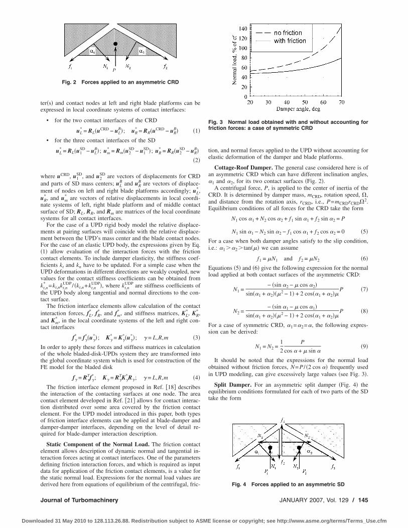
ter�s� and contact nodes at left and right blade platforms can beexpressed in local coordinate systems of contact interfaces:

• for the two contact interfaces of the CRD

uL* = RL�uCRD − uL

B�; uR* = RR�uCRD − uR

B� �1�• for the three contact interfaces of the SD

uL* = RL�u1

SD − uLB�; um

* = Rm�u2SD − u1

SD�; uR* = RR�u2

SD − uRB��2�

where uCRD, u1SD, and u2

SD are vectors of displacements for CRDand parts of SD mass centers; uL

B and uRB are vectors of displace-

ment of nodes on left and right blade platforms accordingly; uL*,

uR* , and um

* are vectors of relative displacements in local coordi-nate systems of left, right blade platform and of middle contactsurface of SD; RL, RR, and Rm are matrices of the local coordinatesystems for all contact interfaces.

For the case of a UPD rigid body model the relative displace-ments at pairing surfaces will coincide with the relative displace-ment between the UPD’s mass center and the blade contact nodes.For the case of an elastic UPD body, the expressions given by Eq.�1� allow evaluation of the interaction forces with the frictioncontact elements. To include damper elasticity, the stiffness coef-ficients kt and kn have to be updated. For a simple case when theUPD deformations in different directions are weakly coupled, newvalues for the contact stiffness coefficients can be obtained fromkt,n

* =kt,nkt,nUDP/ �kt,n+kt,n

UDP�, where kt,nUDP are stiffness coefficients of

the UPD body along tangential and normal directions to the con-tact surface.

The friction interface elements allow calculation of the contactinteraction forces, fL

*, fR* , and fm

* , and stiffness matrices, KL*, KR

* ,and Km

* , in the local coordinate systems of the left and right con-tact interfaces

f�* = f�

*�u�*�; K�

* = K�*�u�

*�; � = L,R,m �3�In order to apply these forces and stiffness matrices in calculationof the whole bladed-disk-UPDs system they are transformed intothe global coordinate system which is used for construction of theFE model for the bladed disk

f� = R�Tf�

* ; K� = R�TK�

*R�; � = L,R,m �4�The friction interface element proposed in Ref. �18� describes

the interaction of the contacting surfaces at one node. The areacontact element developed in Ref. �21� allows for contact interac-tion distributed over some area covered by the friction contactelement. For the UPD model introduced in this paper, both typesof friction interface elements can be applied at blade-damper anddamper-damper interfaces, depending on the level of detail re-quired for blade-damper interaction description.

Static Component of the Normal Load. The friction contactelement allows description of dynamic normal and tangential in-teraction forces acting at contact interfaces. One of the parametersdefining friction interaction forces, and which is required as inputdata for application of the friction contact elements, is a value forthe static normal load. Expressions for the normal load values arederived here from equations of equilibrium of the centrifugal, fric-

tion, and normal forces applied to the UPD without accounting forelastic deformation of the damper and blade platforms.

Cottage-Roof Damper. The general case considered here is ofan asymmetric CRD which can have different inclination angles,�1 and �2, for its two contact surfaces �Fig. 2�.

A centrifugal force, P, is applied to the center of inertia of theCRD. It is determined by damper mass, mCRD, rotation speed, �,and distance from the rotation axis, rCRD, i.e., P=mCRDrCRD�2.Equilibrium conditions of all forces for the CRD take the form

N1 cos �1 + N2 cos �2 + f1 sin �1 + f2 sin �2 = P

N1 sin �1 − N2 sin �2 − f1 cos �1 + f2 cos �2 = 0 �5�For a case when both damper angles satisfy to the slip condition,i.e.: �1��2� tan�� we can assume

f1 = �N1 and f2 = �N2 �6�Equations �5� and �6� give the following expression for the normalload applied at both contact surfaces of the asymmetric CRD:

N1 =− �sin �2 − � cos �2�

sin��1 + �2��2 − 1� + 2 cos��1 + �2��P �7�

N2 =− �sin �1 − � cos �1�

sin��1 + �2��2 − 1� + 2 cos��1 + �2��P �8�

For a case of symmetric CRD, �1=�2=�, the following expres-sion can be derived:

N1 = N2 =1

2

P

cos � + � sin ��9�

It should be noted that the expressions for the normal loadobtained without friction forces, N= P / �2 cos �� frequently usedin UPD modeling, can give excessively large values �see Fig. 3�.

Split Damper. For an asymmetric split damper �Fig. 4� theequilibrium conditions formulated for each of two parts of the SDtake the form

Fig. 2 Forces applied to an asymmetric CRD

Fig. 3 Normal load obtained with and without accounting forfriction forces: a case of symmetric CRD

Fig. 4 Forces applied to an asymmetric SD



• left part

N1 cos �1 + f1 sin �1 + fs = P1

N1 sin �1 − f1 cos �1 − Ns = 0 �10�• right part

N2 cos �2 + f2 sin �2 − fs = P2

− N2 sin �2 + f2 cos �2 + Ns = 0 �11�

where P1 and P2 are the centrifugal forces applied to the two partsof the damper. Additional constraints on tangential forces shouldbe applied in the form of the following inequalities:

�f1� � �N1, �f2� � �N2, �fs� � �Ns �12�

One can see that the system of equations thus produced is un-derdetermined since there are six unknowns in four equations and,hence, it does not generally have a unique solution. For the gen-eral case of an asymmetric SD, these linear equations have to besolved numerically together with the constraints imposed on thefriction forces. Assuming that the masses of both parts of thedamper are proportional to the area of the damper cross section�which is displayed by two triangles in Fig. 4� and that both thedamper angles satisfy to the slip condition: �1��2� tan��; wecan obtain the following expressions for the normal load at themiddle contact surfaces:

• for an asymmetric split damper

Ns =1

2P

cos��1 + �2��1 − �2� − cos��1 − �2��1 + �2� + 2 sin��1 + �2��sin��1 + �2��2 − 1� + 2 cos��1 + �2��

�13�

• for a symmetric split damper

Ns =1

2

P�sin � − � cos ��cos � + � sin �

�14�

where P= P1+ P2 is a total centrifugal force produced by the SD.Expressions for the normal loads at the other two contact surfacesare given for an asymmetric SD by Eqs. �7� and �8�, and for thesymmetric SD by Eq. �9�.

Method for Forced Response AnalysisA bladed disk with UPDs is essentially a nonlinear structure.

For a search of the steady-state periodic nonlinear forced re-sponse, the time variation of all DOFs in the model of a bladeddisk with UPDs is represented by a restricted Fourier series

q�t� = Q0 + �j=1

n

�Q j�c�cos mj�t + Q j

�s�sin mj�t� �15�

where q�t� is a vector comprising time variation of DOFs; Q j�c�

and Q j�s� �j=1, . . . ,n� are vectors of cosine and sine harmonic

coefficients for system DOFs, marked by superscripts �c� and �s�

accordingly; Q0 is a vector of constant components of the dis-placements; mj are specific numbers of harmonics that are kept inthe displacement expansion.

Application of the multiharmonic balance method and conden-sation techniques described in Refs. �19,20� gives an equation ofmotion in the frequency domain with respect to the harmoniccoefficients of a multiharmonic expansion in the form

R�Q,�,�� = Q + A��F�Q,b�� − P�� = 0 �16�

where Q= �Q0 ,Q1�c� ,Q1

�s� , . . . ,Qn�s��T is a vector of harmonic coef-

ficients of displacements; P= �P0 ,P1�c� ,P1

�s� , . . . ,Pn�s��T is a vector

of harmonic components of the excitation forces; F�Q ,b��= �F0 ,F1

�c� ,F1�s� , . . . ,Fn

�s��T is a vector of harmonic components ofnonlinear forces applied at contact interfaces, and A�� is a mul-tiharmonic FRF matrix of the linear part of the system, i.e.,

A�� = diag�A0,A1��, . . . ,An�� 17�

where FRF matrices for each harmonic, A j��, can be generatedfrom mode shapes and natural frequencies obtained for a linearstructure without contact interactions. The solution of nonlinearEq. �16� and the tracing of solutions when rotation speed, excita-

tion frequency, or UPD’s parameters are varied is performed usingmethods reported in Refs. �19,20,22�.

Test Case StudiesA blisk of 24 blades, which is analyzed here, was manufactured

for a test rig built at Imperial College London in the framework ofthe EU project “Aeroelastic Design of Turbine Blades II”�ADTurbII� �see Ref. �23��. A finite element model of this blisk isshown in Fig. 5.

Two types of UPD are analyzed: �i� cottage-roof dampers and�ii� split dampers. The case of a tuned blisc is analyzed here andidentical UPDs are applied to all sectors of the bladed disk. A FEmodel of one sector of the blisk used in calculation contains21,555 DOFs. The natural frequencies—nodal diameters diagramfor this bladed disk are given in Ref. �24�. The background damp-ing due to damping in the blisk material is assumed to be low:=7.5e−05. Dissipation of vibration energy due to friction forcesproduced by UPDs is calculated together with the forced responsecalculation. A traveling wave excitation pattern of 19th engineorder is applied to the blisk in the forced response calculations.Five harmonics, which are the first five odd multiples of the 19thengine order �i.e., 19, 57, 95, 133, and 171�, are used in the mul-tiharmonic expansion of displacements for the calculations per-formed here.

Cottage-Roof Dampers. Numerical investigations were per-formed for the case of a symmetric CRD of prismatic shape �Fig.5�b��. The CRD was inserted into the specially machined slotsunderneath the blade platforms. The slots are inclined to the rota-tion axis by approximately 30 deg. The effects of parameters of

Fig. 5 FE model of a blisc and UPD’s models studied



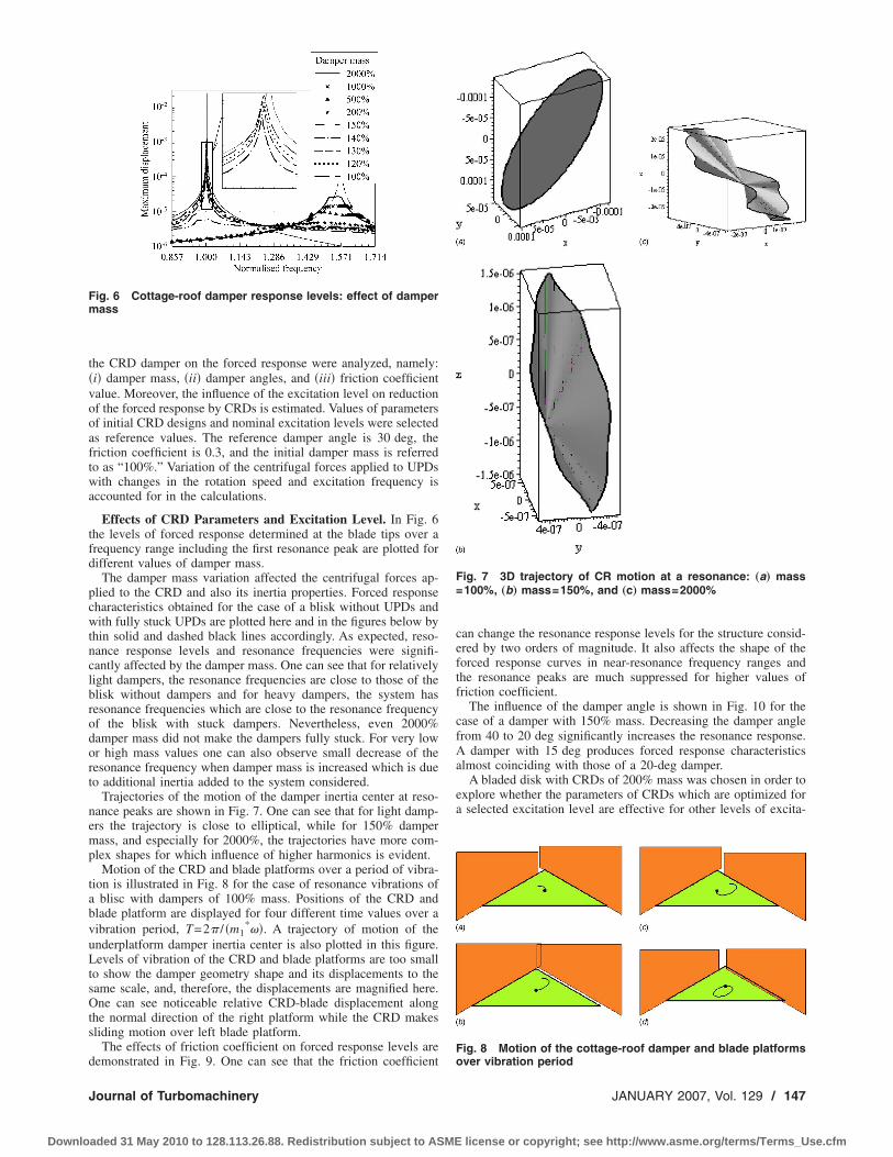
the CRD damper on the forced response were analyzed, namely:�i� damper mass, �ii� damper angles, and �iii� friction coefficientvalue. Moreover, the influence of the excitation level on reductionof the forced response by CRDs is estimated. Values of parametersof initial CRD designs and nominal excitation levels were selectedas reference values. The reference damper angle is 30 deg, thefriction coefficient is 0.3, and the initial damper mass is referredto as “100%.” Variation of the centrifugal forces applied to UPDswith changes in the rotation speed and excitation frequency isaccounted for in the calculations.

Effects of CRD Parameters and Excitation Level. In Fig. 6the levels of forced response determined at the blade tips over afrequency range including the first resonance peak are plotted fordifferent values of damper mass.

The damper mass variation affected the centrifugal forces ap-plied to the CRD and also its inertia properties. Forced responsecharacteristics obtained for the case of a blisk without UPDs andwith fully stuck UPDs are plotted here and in the figures below bythin solid and dashed black lines accordingly. As expected, reso-nance response levels and resonance frequencies were signifi-cantly affected by the damper mass. One can see that for relativelylight dampers, the resonance frequencies are close to those of theblisk without dampers and for heavy dampers, the system hasresonance frequencies which are close to the resonance frequencyof the blisk with stuck dampers. Nevertheless, even 2000%damper mass did not make the dampers fully stuck. For very lowor high mass values one can also observe small decrease of theresonance frequency when damper mass is increased which is dueto additional inertia added to the system considered.

Trajectories of the motion of the damper inertia center at reso-nance peaks are shown in Fig. 7. One can see that for light damp-ers the trajectory is close to elliptical, while for 150% dampermass, and especially for 2000%, the trajectories have more com-plex shapes for which influence of higher harmonics is evident.

Motion of the CRD and blade platforms over a period of vibra-tion is illustrated in Fig. 8 for the case of resonance vibrations ofa blisc with dampers of 100% mass. Positions of the CRD andblade platform are displayed for four different time values over avibration period, T=2 / �m1

*��. A trajectory of motion of theunderplatform damper inertia center is also plotted in this figure.Levels of vibration of the CRD and blade platforms are too smallto show the damper geometry shape and its displacements to thesame scale, and, therefore, the displacements are magnified here.One can see noticeable relative CRD-blade displacement alongthe normal direction of the right platform while the CRD makessliding motion over left blade platform.

The effects of friction coefficient on forced response levels aredemonstrated in Fig. 9. One can see that the friction coefficient

can change the resonance response levels for the structure consid-ered by two orders of magnitude. It also affects the shape of theforced response curves in near-resonance frequency ranges andthe resonance peaks are much suppressed for higher values offriction coefficient.

The influence of the damper angle is shown in Fig. 10 for thecase of a damper with 150% mass. Decreasing the damper anglefrom 40 to 20 deg significantly increases the resonance response.A damper with 15 deg produces forced response characteristicsalmost coinciding with those of a 20-deg damper.

A bladed disk with CRDs of 200% mass was chosen in order toexplore whether the parameters of CRDs which are optimized fora selected excitation level are effective for other levels of excita-

Fig. 6 Cottage-roof damper response levels: effect of dampermass

Fig. 7 3D trajectory of CR motion at a resonance: „a… mass=100%, „b… mass=150%, and „c… mass=2000%

Fig. 8 Motion of the cottage-roof damper and blade platformsover vibration period



tion. The 200% damper mass value was chosen because it pro-duced the lowest level of the forced response for 100% excitationlevel �see Fig. 6�. In Fig. 11 the forced response levels are plottedfor a blisk with such CRDs for several different levels of excita-tion from 100% to 200%. One can see that although the damper isoptimal for the excitation level of 100%, for higher levels of ex-citation the forced response curve becomes similar to the cases oflighter dampers under 100% excitation and the damper mass is notalready optimal for this excitation level.

The effects of UPD parameters and the excitation level on theresonance forced response level are summarized in Fig. 12, whichshows a high sensitivity of the resonance peak responses to theparameter values and helps in the choice of the optimal parametervalues.

Multiharmonic Spectrum of the Forced Response. Due tothe nonlinear character of the blade-UPD interactions, the forcedresponse spectrum is essentially multiharmonic, even when mono-

harmonic excitation forces are applied. Spectra of the forced re-sponse calculated over the whole frequency range analyzed areshown in Figs. 13 and 14. The forced response spectra are plottedfor two differently located nodes: �i� at the blade tip and �ii� at the

Fig. 9 Cottage-roof damper response levels: effect of frictioncoefficient „mass=100%, angle=30 deg…

Fig. 10 Cottage-roof damper response levels: effect ofdamper angle „mass=150% …

Fig. 11 Cottage-roof damper response levels: effect of excita-tion level „mass=200%, angle=30 deg…

Fig. 12 Cottage-roof damper: resonance peak levels as func-tions of the damper parameters

Fig. 13 Amplitudes of harmonics of the multiharmonic forcedresponse „mass=100% …: „a… at the blade tip and „b… for CRdamper motion



UPD inertia center.Two cases are considered: �i� the case of a light UPD �mass

=100%, Fig. 13� and �ii� the case of heavy damper �mass=2000%, Fig. 14�. One can see that for a blade tip displacement,the first harmonic is dominant for both cases displayed here. Forthe UPD displacement, the contributions of higher harmonics aresignificant. For the case of a heavy damper, the higher harmonic

amplitudes are close to that of the first harmonic.Since contact interface interactions are determined by motion of

the UPD and the blade platforms accounting for these higher har-monics is essential to determine accurately the forces at UPDcontact interfaces. When higher harmonics are significant, the tra-jectory of UPD motion has a complex shape �see Figs. 7�b� and7�c�� which is different from conventional ellipsoidal shape inher-ent for monoharmonic motion. Errors in predictions of resonancepeak forced response when monoharmonic forced response repre-sentation is used are shown in Fig. 15 where results of the multi-harmonic analysis are used for reference values.

Split Damper. Forced responses of a blisk with split dampersare shown in Fig. 16 for different values of damper mass. Forcomparison, forced response levels of the blisc with CRDs areplotted there, also. One can see that the SD is more efficient inreducing the response levels for heavy dampers and less efficient

Fig. 14 Amplitudes of harmonics of the multiharmonic forcedresponse „mass=2000% …: „a… at the blade tip and „b… for CRdamper motion

Fig. 15 Error in prediction of the resonance response levelswhen only one harmonic is allowed for

Fig. 16 Comparison of response levels for a blisk with CRDand SD for different damper mass values

Fig. 17 Resonance peak response for a blisk with CRD and SDfor different damper mass values

Fig. 18 3D trajectories of motion for two parts of the splitdamper: „a… mass=100%, „b… mass=2000%



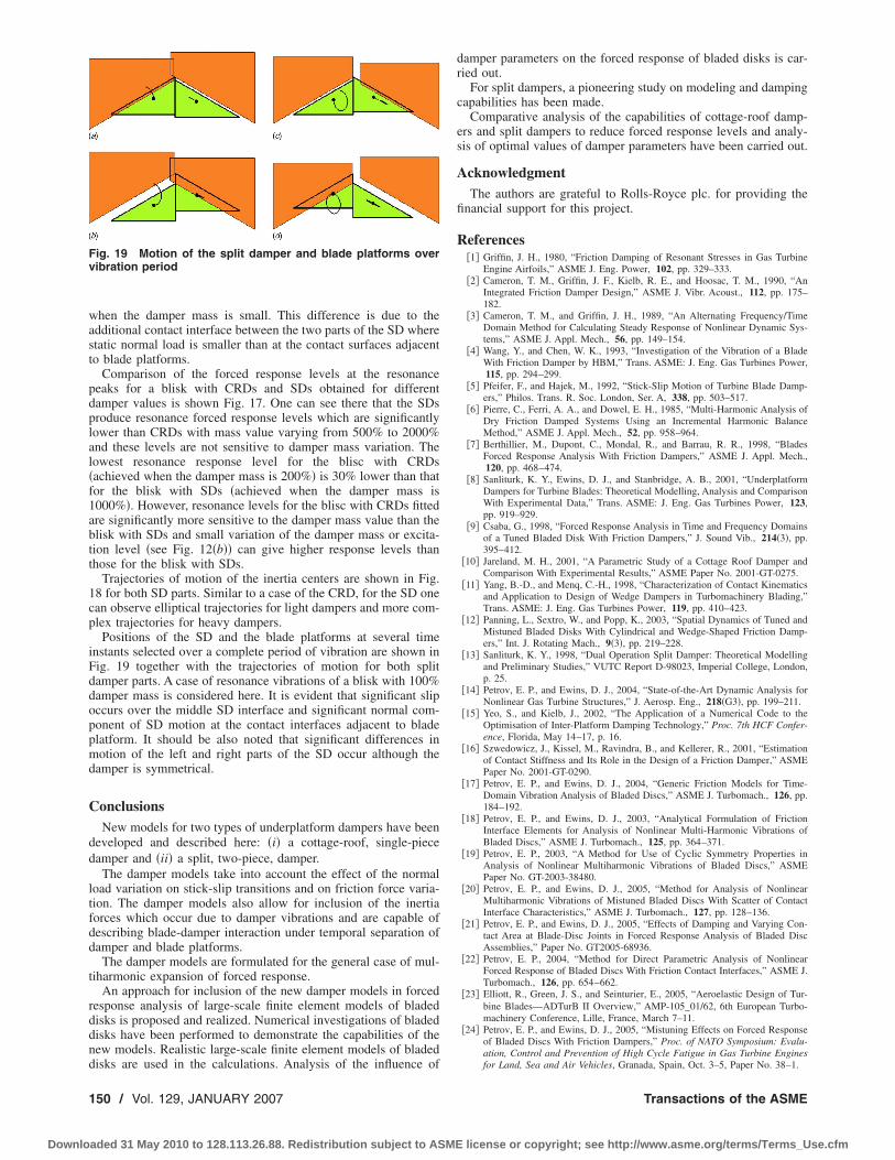
when the damper mass is small. This difference is due to theadditional contact interface between the two parts of the SD wherestatic normal load is smaller than at the contact surfaces adjacentto blade platforms.

Comparison of the forced response levels at the resonancepeaks for a blisk with CRDs and SDs obtained for differentdamper values is shown Fig. 17. One can see there that the SDsproduce resonance forced response levels which are significantlylower than CRDs with mass value varying from 500% to 2000%and these levels are not sensitive to damper mass variation. Thelowest resonance response level for the blisc with CRDs�achieved when the damper mass is 200%� is 30% lower than thatfor the blisk with SDs �achieved when the damper mass is1000%�. However, resonance levels for the blisc with CRDs fittedare significantly more sensitive to the damper mass value than theblisk with SDs and small variation of the damper mass or excita-tion level �see Fig. 12�b�� can give higher response levels thanthose for the blisk with SDs.

Trajectories of motion of the inertia centers are shown in Fig.18 for both SD parts. Similar to a case of the CRD, for the SD onecan observe elliptical trajectories for light dampers and more com-plex trajectories for heavy dampers.

Positions of the SD and the blade platforms at several timeinstants selected over a complete period of vibration are shown inFig. 19 together with the trajectories of motion for both splitdamper parts. A case of resonance vibrations of a blisk with 100%damper mass is considered here. It is evident that significant slipoccurs over the middle SD interface and significant normal com-ponent of SD motion at the contact interfaces adjacent to bladeplatform. It should be also noted that significant differences inmotion of the left and right parts of the SD occur although thedamper is symmetrical.

ConclusionsNew models for two types of underplatform dampers have been

developed and described here: �i� a cottage-roof, single-piecedamper and �ii� a split, two-piece, damper.

The damper models take into account the effect of the normalload variation on stick-slip transitions and on friction force varia-tion. The damper models also allow for inclusion of the inertiaforces which occur due to damper vibrations and are capable ofdescribing blade-damper interaction under temporal separation ofdamper and blade platforms.

The damper models are formulated for the general case of mul-tiharmonic expansion of forced response.

An approach for inclusion of the new damper models in forcedresponse analysis of large-scale finite element models of bladeddisks is proposed and realized. Numerical investigations of bladeddisks have been performed to demonstrate the capabilities of thenew models. Realistic large-scale finite element models of bladeddisks are used in the calculations. Analysis of the influence of

damper parameters on the forced response of bladed disks is car-ried out.

For split dampers, a pioneering study on modeling and dampingcapabilities has been made.

Comparative analysis of the capabilities of cottage-roof damp-ers and split dampers to reduce forced response levels and analy-sis of optimal values of damper parameters have been carried out.

AcknowledgmentThe authors are grateful to Rolls-Royce plc. for providing the

financial support for this project.

References�1� Griffin, J. H., 1980, “Friction Damping of Resonant Stresses in Gas Turbine

Engine Airfoils,” ASME J. Eng. Power, 102, pp. 329–333.�2� Cameron, T. M., Griffin, J. F., Kielb, R. E., and Hoosac, T. M., 1990, “An

Integrated Friction Damper Design,” ASME J. Vibr. Acoust., 112, pp. 175–182.

�3� Cameron, T. M., and Griffin, J. H., 1989, “An Alternating Frequency/TimeDomain Method for Calculating Steady Response of Nonlinear Dynamic Sys-tems,” ASME J. Appl. Mech., 56, pp. 149–154.

�4� Wang, Y., and Chen, W. K., 1993, “Investigation of the Vibration of a BladeWith Friction Damper by HBM,” Trans. ASME: J. Eng. Gas Turbines Power,115, pp. 294–299.

�5� Pfeifer, F., and Hajek, M., 1992, “Stick-Slip Motion of Turbine Blade Damp-ers,” Philos. Trans. R. Soc. London, Ser. A, 338, pp. 503–517.

�6� Pierre, C., Ferri, A. A., and Dowel, E. H., 1985, “Multi-Harmonic Analysis ofDry Friction Damped Systems Using an Incremental Harmonic BalanceMethod,” ASME J. Appl. Mech., 52, pp. 958–964.

�7� Berthillier, M., Dupont, C., Mondal, R., and Barrau, R. R., 1998, “BladesForced Response Analysis With Friction Dampers,” ASME J. Appl. Mech.,120, pp. 468–474.

�8� Sanliturk, K. Y., Ewins, D. J., and Stanbridge, A. B., 2001, “UnderplatformDampers for Turbine Blades: Theoretical Modelling, Analysis and ComparisonWith Experimental Data,” Trans. ASME: J. Eng. Gas Turbines Power, 123,pp. 919–929.

�9� Csaba, G., 1998, “Forced Response Analysis in Time and Frequency Domainsof a Tuned Bladed Disk With Friction Dampers,” J. Sound Vib., 214�3�, pp.395–412.

�10� Jareland, M. H., 2001, “A Parametric Study of a Cottage Roof Damper andComparison With Experimental Results,” ASME Paper No. 2001-GT-0275.

�11� Yang, B.-D., and Menq, C.-H., 1998, “Characterization of Contact Kinematicsand Application to Design of Wedge Dampers in Turbomachinery Blading,”Trans. ASME: J. Eng. Gas Turbines Power, 119, pp. 410–423.

�12� Panning, L., Sextro, W., and Popp, K., 2003, “Spatial Dynamics of Tuned andMistuned Bladed Disks With Cylindrical and Wedge-Shaped Friction Damp-ers,” Int. J. Rotating Mach., 9�3�, pp. 219–228.

�13� Sanliturk, K. Y., 1998, “Dual Operation Split Damper: Theoretical Modellingand Preliminary Studies,” VUTC Report D-98023, Imperial College, London,p. 25.

�14� Petrov, E. P., and Ewins, D. J., 2004, “State-of-the-Art Dynamic Analysis forNonlinear Gas Turbine Structures,” J. Aerosp. Eng., 218�G3�, pp. 199–211.

�15� Yeo, S., and Kielb, J., 2002, “The Application of a Numerical Code to theOptimisation of Inter-Platform Damping Technology,” Proc. 7th HCF Confer-ence, Florida, May 14–17, p. 16.

�16� Szwedowicz, J., Kissel, M., Ravindra, B., and Kellerer, R., 2001, “Estimationof Contact Stiffness and Its Role in the Design of a Friction Damper,” ASMEPaper No. 2001-GT-0290.

�17� Petrov, E. P., and Ewins, D. J., 2004, “Generic Friction Models for Time-Domain Vibration Analysis of Bladed Discs,” ASME J. Turbomach., 126, pp.184–192.

�18� Petrov, E. P., and Ewins, D. J., 2003, “Analytical Formulation of FrictionInterface Elements for Analysis of Nonlinear Multi-Harmonic Vibrations ofBladed Discs,” ASME J. Turbomach., 125, pp. 364–371.

�19� Petrov, E. P., 2003, “A Method for Use of Cyclic Symmetry Properties inAnalysis of Nonlinear Multiharmonic Vibrations of Bladed Discs,” ASMEPaper No. GT-2003-38480.

�20� Petrov, E. P., and Ewins, D. J., 2005, “Method for Analysis of NonlinearMultiharmonic Vibrations of Mistuned Bladed Discs With Scatter of ContactInterface Characteristics,” ASME J. Turbomach., 127, pp. 128–136.

�21� Petrov, E. P., and Ewins, D. J., 2005, “Effects of Damping and Varying Con-tact Area at Blade-Disc Joints in Forced Response Analysis of Bladed DiscAssemblies,” Paper No. GT2005-68936.

�22� Petrov, E. P., 2004, “Method for Direct Parametric Analysis of NonlinearForced Response of Bladed Discs With Friction Contact Interfaces,” ASME J.Turbomach., 126, pp. 654–662.

�23� Elliott, R., Green, J. S., and Seinturier, E., 2005, “Aeroelastic Design of Tur-bine Blades—ADTurB II Overview,” AMP-105_01/62, 6th European Turbo-machinery Conference, Lille, France, March 7–11.

�24� Petrov, E. P., and Ewins, D. J., 2005, “Mistuning Effects on Forced Responseof Bladed Discs With Friction Dampers,” Proc. of NATO Symposium: Evalu-ation, Control and Prevention of High Cycle Fatigue in Gas Turbine Enginesfor Land, Sea and Air Vehicles, Granada, Spain, Oct. 3–5, Paper No. 38–1.

Fig. 19 Motion of the split damper and blade platforms overvibration period



Hasan Nasir

Srinath V. Ekkad1

ProfessorMem. ASME


Mechanical Engineering Department,Louisiana State University,

Baton Rouge, LA 70803

Ronald S. BunkerGeneral Electric Global R&D Center,

Schenectady, NY

Effect of Tip and Pressure SideCoolant Injection on Heat TransferDistributions for a Plane andRecessed TipThe present study investigates the effects of coolant injection on adiabatic film effective-ness and heat transfer coefficients from a plane and recessed tip of a high pressureturbine first stage rotor blade. Three cases where coolant is injected from (a) five or-thogonal holes located along the camber line, (b) seven angled holes located near theblade tip along the pressure side, and (c) combination cases when coolant is injectedfrom both tip and pressure side holes were studied. The pressure ratio (inlet total pressureto exit static pressure for the cascade) across the blade row was 1.2, and the experimentswere run in a blow-down test rig with a four-blade linear cascade. The Reynolds numberbased on cascade exit velocity and axial chord length was 8.61�105 and the inlet andexit Mach numbers were 0.16 and 0.55, respectively. A transient infrared technique wasused to measure adiabatic film effectiveness and heat transfer coefficient simultaneouslyfor three blowing ratios of 1.0, 2.0, and 3.0. For all the cases, gap-to-blade span ratio of1% was used. The depth-to-blade span ratio of 0.0416 was used for the recessed tip.Pressure measurements on the shroud were also taken to characterize the leakage flowand understand the heat transfer distributions. For tip injection, when blowing ratioincreases from 1.0 to 2.0, film effectiveness increases for both plane and recessed tip andheat transfer coefficient decreases for both plane and recessed tip. At blowing ratio 3.0,lift-off is observed for both cases. In case of pressure side coolant injection and for planetip, lift-off is observed at blowing ratio 2.0 and reattachments of jets are observed atblowing ratio 3.0. But, almost no effectiveness is observed for squealer tip at all blowingratios with pressure side injection with reduced heat transfer coefficient along the pres-sure side. For combination case, very high effectiveness is observed at blowing ratio 3.0for both plane and recessed blade tip. It appears that for this high blowing ratio, coolantjets from the tip hit the shroud first and then reattach back onto the blade tip with veryhigh heat transfer coefficients for both plane and recessed blade tip.�DOI: 10.1115/1.2366540�

IntroductionModern turbine blades are exposed to increasingly high inlet

temperatures. The high pressure turbine �HPT� first stage blade issubject to extremely harsh environments. Most failures in bladesoccur at the turbine tip region due to over-temperature and coolingproblems. The tip region through exposure to hot leakage gasesleads to loss of performance and life through oxidation, erosion,rubbing against stationary outer casing, and high local thermalstresses.

The cause for tip failures is fairly well understood and can beexplained as follows. A clearance gap between the rotating bladetip and stationary shroud is necessary to allow for the blade’smechanical and thermal growth during operation. Unfortunately,the gap allows for leakage flow from the pressure side to thesuction side of the blade surface. The gas accelerates as it passesthrough the small gap. This leads to enhanced heat load to theblade tip region. Leakage flow, or clearance flow, also leads toundesirable aerodynamic losses. In fact, one third of the aerody-namic losses through the turbine section can be attributed to leak-age flow. The effects of leakage flow are increased thermal load-

ing and reduced aerodynamic performance, which affectsdurability and life of the component. At these elevated tempera-tures, the turbine blades are also at risk of undergoing oxidation,thermal barrier coating �TBC� spallation, thermal fatigue, andcreep. Tip region is difficult to cool with conventional internalcooling because of the difficulty of producing high internal heattransfer coefficients to effectively reduce tip region thermal load-ing. Typically, coolant is injected into the tip gap to reduce theheat loading by reducing overall leakage flow temperature. Also,coolant is injected along the pressure side surface of the bladeclose to the tip gap. However, the lack of flow field knowledgeand accurate local thermal distribution on the tip region results inineffective cooling. This study looks at heat transfer measure-ments on cooled tips with typical cooling hole placements as seenin an in-service engine blade.

An overview of the tip heat transfer through different sealingmechanisms is presented in detail by Nasir et al. �1�. Severaldifferent geometries such as trip strips and recessed cavity geom-etry were examined for reducing leakage flow and associated heattransfer. However, film cooling of the tips still remains a majorneed as tip temperatures are significant. Film injection on the tipsurface has been primarily through dust/purge holes in conven-tional designs. These are metered holes that release some coolantto the tip to remove collection of dust inside the internal passagesof the blades. However, with increased problems in the tip region,tip holes were also used to deliver coolant to the tip gap region toreduce the leakage flow and provide cooling. Recently, there have

1Corresponding author.Contributed by the International Gas Turbine Institute �IGTI� of ASME for pub-

lication in the JOURNAL OF TURBOMACHINERY. Manuscript received October 1, 2004;final manuscript received February 1, 2005. IGTI Review Chair: K. C. Hall. Paperpresented at the ASME Turbo Expo 2005: Land, Sea and Air, Reno, NV, June 6–9,2005, Paper No. GT2005-68595.



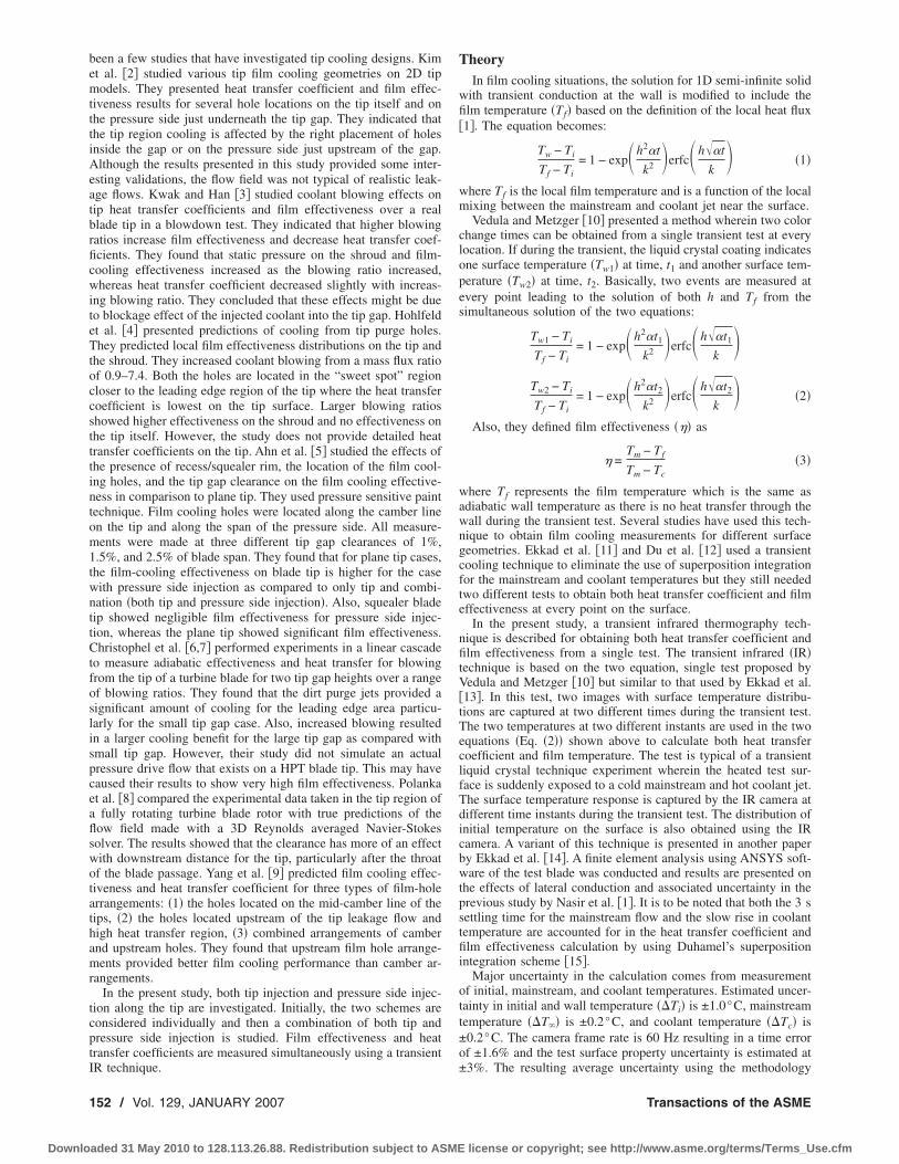
been a few studies that have investigated tip cooling designs. Kimet al. �2� studied various tip film cooling geometries on 2D tipmodels. They presented heat transfer coefficient and film effec-tiveness results for several hole locations on the tip itself and onthe pressure side just underneath the tip gap. They indicated thatthe tip region cooling is affected by the right placement of holesinside the gap or on the pressure side just upstream of the gap.Although the results presented in this study provided some inter-esting validations, the flow field was not typical of realistic leak-age flows. Kwak and Han �3� studied coolant blowing effects ontip heat transfer coefficients and film effectiveness over a realblade tip in a blowdown test. They indicated that higher blowingratios increase film effectiveness and decrease heat transfer coef-ficients. They found that static pressure on the shroud and film-cooling effectiveness increased as the blowing ratio increased,whereas heat transfer coefficient decreased slightly with increas-ing blowing ratio. They concluded that these effects might be dueto blockage effect of the injected coolant into the tip gap. Hohlfeldet al. �4� presented predictions of cooling from tip purge holes.They predicted local film effectiveness distributions on the tip andthe shroud. They increased coolant blowing from a mass flux ratioof 0.9–7.4. Both the holes are located in the “sweet spot” regioncloser to the leading edge region of the tip where the heat transfercoefficient is lowest on the tip surface. Larger blowing ratiosshowed higher effectiveness on the shroud and no effectiveness onthe tip itself. However, the study does not provide detailed heattransfer coefficients on the tip. Ahn et al. �5� studied the effects ofthe presence of recess/squealer rim, the location of the film cool-ing holes, and the tip gap clearance on the film cooling effective-ness in comparison to plane tip. They used pressure sensitive painttechnique. Film cooling holes were located along the camber lineon the tip and along the span of the pressure side. All measure-ments were made at three different tip gap clearances of 1%,1.5%, and 2.5% of blade span. They found that for plane tip cases,the film-cooling effectiveness on blade tip is higher for the casewith pressure side injection as compared to only tip and combi-nation �both tip and pressure side injection�. Also, squealer bladetip showed negligible film effectiveness for pressure side injec-tion, whereas the plane tip showed significant film effectiveness.Christophel et al. �6,7� performed experiments in a linear cascadeto measure adiabatic effectiveness and heat transfer for blowingfrom the tip of a turbine blade for two tip gap heights over a rangeof blowing ratios. They found that the dirt purge jets provided asignificant amount of cooling for the leading edge area particu-larly for the small tip gap case. Also, increased blowing resultedin a larger cooling benefit for the large tip gap as compared withsmall tip gap. However, their study did not simulate an actualpressure drive flow that exists on a HPT blade tip. This may havecaused their results to show very high film effectiveness. Polankaet al. �8� compared the experimental data taken in the tip region ofa fully rotating turbine blade rotor with true predictions of theflow field made with a 3D Reynolds averaged Navier-Stokessolver. The results showed that the clearance has more of an effectwith downstream distance for the tip, particularly after the throatof the blade passage. Yang et al. �9� predicted film cooling effec-tiveness and heat transfer coefficient for three types of film-holearrangements: �1� the holes located on the mid-camber line of thetips, �2� the holes located upstream of the tip leakage flow andhigh heat transfer region, �3� combined arrangements of camberand upstream holes. They found that upstream film hole arrange-ments provided better film cooling performance than camber ar-rangements.

In the present study, both tip injection and pressure side injec-tion along the tip are investigated. Initially, the two schemes areconsidered individually and then a combination of both tip andpressure side injection is studied. Film effectiveness and heattransfer coefficients are measured simultaneously using a transientIR technique.

TheoryIn film cooling situations, the solution for 1D semi-infinite solid

with transient conduction at the wall is modified to include thefilm temperature �Tf� based on the definition of the local heat flux�1�. The equation becomes:

Tw − Ti

Tf − Ti= 1 − exp�h2�t

k2 �erfc�h��t

k� �1�

where Tf is the local film temperature and is a function of the localmixing between the mainstream and coolant jet near the surface.

Vedula and Metzger �10� presented a method wherein two colorchange times can be obtained from a single transient test at everylocation. If during the transient, the liquid crystal coating indicatesone surface temperature �Tw1� at time, t1 and another surface tem-perature �Tw2� at time, t2. Basically, two events are measured atevery point leading to the solution of both h and Tf from thesimultaneous solution of the two equations:

Tw1 − Ti

Tf − Ti= 1 − exp�h2�t1

k2 �erfc�h��t1

k�

Tw2 − Ti

Tf − Ti= 1 − exp�h2�t2

k2 �erfc�h��t2

k� �2�

Also, they defined film effectiveness �� as

� =Tm − Tf

Tm − Tc�3�

where Tf represents the film temperature which is the same asadiabatic wall temperature as there is no heat transfer through thewall during the transient test. Several studies have used this tech-nique to obtain film cooling measurements for different surfacegeometries. Ekkad et al. �11� and Du et al. �12� used a transientcooling technique to eliminate the use of superposition integrationfor the mainstream and coolant temperatures but they still neededtwo different tests to obtain both heat transfer coefficient and filmeffectiveness at every point on the surface.

In the present study, a transient infrared thermography tech-nique is described for obtaining both heat transfer coefficient andfilm effectiveness from a single test. The transient infrared �IR�technique is based on the two equation, single test proposed byVedula and Metzger �10� but similar to that used by Ekkad et al.�13�. In this test, two images with surface temperature distribu-tions are captured at two different times during the transient test.The two temperatures at two different instants are used in the twoequations �Eq. �2�� shown above to calculate both heat transfercoefficient and film temperature. The test is typical of a transientliquid crystal technique experiment wherein the heated test sur-face is suddenly exposed to a cold mainstream and hot coolant jet.The surface temperature response is captured by the IR camera atdifferent time instants during the transient test. The distribution ofinitial temperature on the surface is also obtained using the IRcamera. A variant of this technique is presented in another paperby Ekkad et al. �14�. A finite element analysis using ANSYS soft-ware of the test blade was conducted and results are presented onthe effects of lateral conduction and associated uncertainty in theprevious study by Nasir et al. �1�. It is to be noted that both the 3 ssettling time for the mainstream flow and the slow rise in coolanttemperature are accounted for in the heat transfer coefficient andfilm effectiveness calculation by using Duhamel’s superpositionintegration scheme �15�.

Major uncertainty in the calculation comes from measurementof initial, mainstream, and coolant temperatures. Estimated uncer-tainty in initial and wall temperature ��Ti� is ±1.0°C, mainstreamtemperature ��T�� is ±0.2°C, and coolant temperature ��Tc� is±0.2°C. The camera frame rate is 60 Hz resulting in a time errorof ±1.6% and the test surface property uncertainty is estimated at±3%. The resulting average uncertainty using the methodology



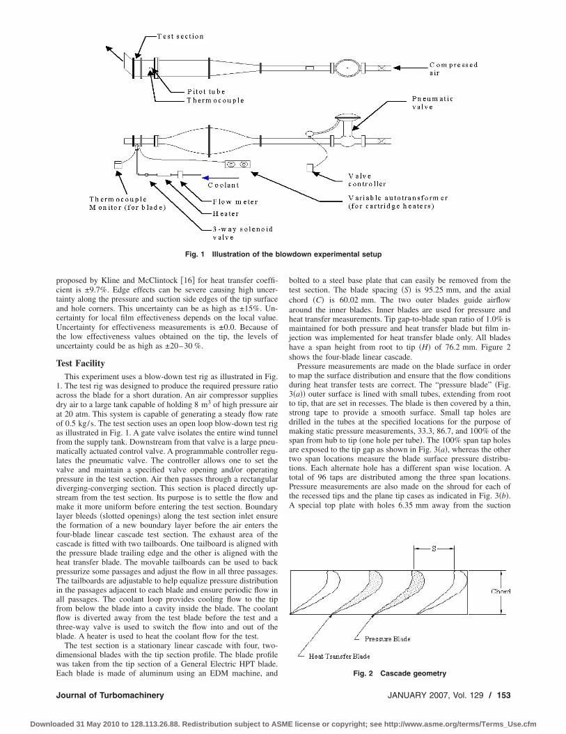
proposed by Kline and McClintock �16� for heat transfer coeffi-cient is ±9.7%. Edge effects can be severe causing high uncer-tainty along the pressure and suction side edges of the tip surfaceand hole corners. This uncertainty can be as high as ±15%. Un-certainty for local film effectiveness depends on the local value.Uncertainty for effectiveness measurements is ±0.0. Because ofthe low effectiveness values obtained on the tip, the levels ofuncertainty could be as high as ±20–30 %.

Test FacilityThis experiment uses a blow-down test rig as illustrated in Fig.

1. The test rig was designed to produce the required pressure ratioacross the blade for a short duration. An air compressor suppliesdry air to a large tank capable of holding 8 m3 of high pressure airat 20 atm. This system is capable of generating a steady flow rateof 0.5 kg/s. The test section uses an open loop blow-down test rigas illustrated in Fig. 1. A gate valve isolates the entire wind tunnelfrom the supply tank. Downstream from that valve is a large pneu-matically actuated control valve. A programmable controller regu-lates the pneumatic valve. The controller allows one to set thevalve and maintain a specified valve opening and/or operatingpressure in the test section. Air then passes through a rectangulardiverging-converging section. This section is placed directly up-stream from the test section. Its purpose is to settle the flow andmake it more uniform before entering the test section. Boundarylayer bleeds �slotted openings� along the test section inlet ensurethe formation of a new boundary layer before the air enters thefour-blade linear cascade test section. The exhaust area of thecascade is fitted with two tailboards. One tailboard is aligned withthe pressure blade trailing edge and the other is aligned with theheat transfer blade. The movable tailboards can be used to backpressurize some passages and adjust the flow in all three passages.The tailboards are adjustable to help equalize pressure distributionin the passages adjacent to each blade and ensure periodic flow inall passages. The coolant loop provides cooling flow to the tipfrom below the blade into a cavity inside the blade. The coolantflow is diverted away from the test blade before the test and athree-way valve is used to switch the flow into and out of theblade. A heater is used to heat the coolant flow for the test.

The test section is a stationary linear cascade with four, two-dimensional blades with the tip section profile. The blade profilewas taken from the tip section of a General Electric HPT blade.Each blade is made of aluminum using an EDM machine, and

bolted to a steel base plate that can easily be removed from thetest section. The blade spacing �S� is 95.25 mm, and the axialchord �C� is 60.02 mm. The two outer blades guide airflowaround the inner blades. Inner blades are used for pressure andheat transfer measurements. Tip gap-to-blade span ratio of 1.0% ismaintained for both pressure and heat transfer blade but film in-jection was implemented for heat transfer blade only. All bladeshave a span height from root to tip �H� of 76.2 mm. Figure 2shows the four-blade linear cascade.

Pressure measurements are made on the blade surface in orderto map the surface distribution and ensure that the flow conditionsduring heat transfer tests are correct. The “pressure blade” �Fig.3�a�� outer surface is lined with small tubes, extending from rootto tip, that are set in recesses. The blade is then covered by a thin,strong tape to provide a smooth surface. Small tap holes aredrilled in the tubes at the specified locations for the purpose ofmaking static pressure measurements, 33.3, 86.7, and 100% of thespan from hub to tip �one hole per tube�. The 100% span tap holesare exposed to the tip gap as shown in Fig. 3�a�, whereas the othertwo span locations measure the blade surface pressure distribu-tions. Each alternate hole has a different span wise location. Atotal of 96 taps are distributed among the three span locations.Pressure measurements are also made on the shroud for each ofthe recessed tips and the plane tip cases as indicated in Fig. 3�b�.A special top plate with holes 6.35 mm away from the suction

Fig. 1 Illustration of the blowdown experimental setup

Fig. 2 Cascade geometry



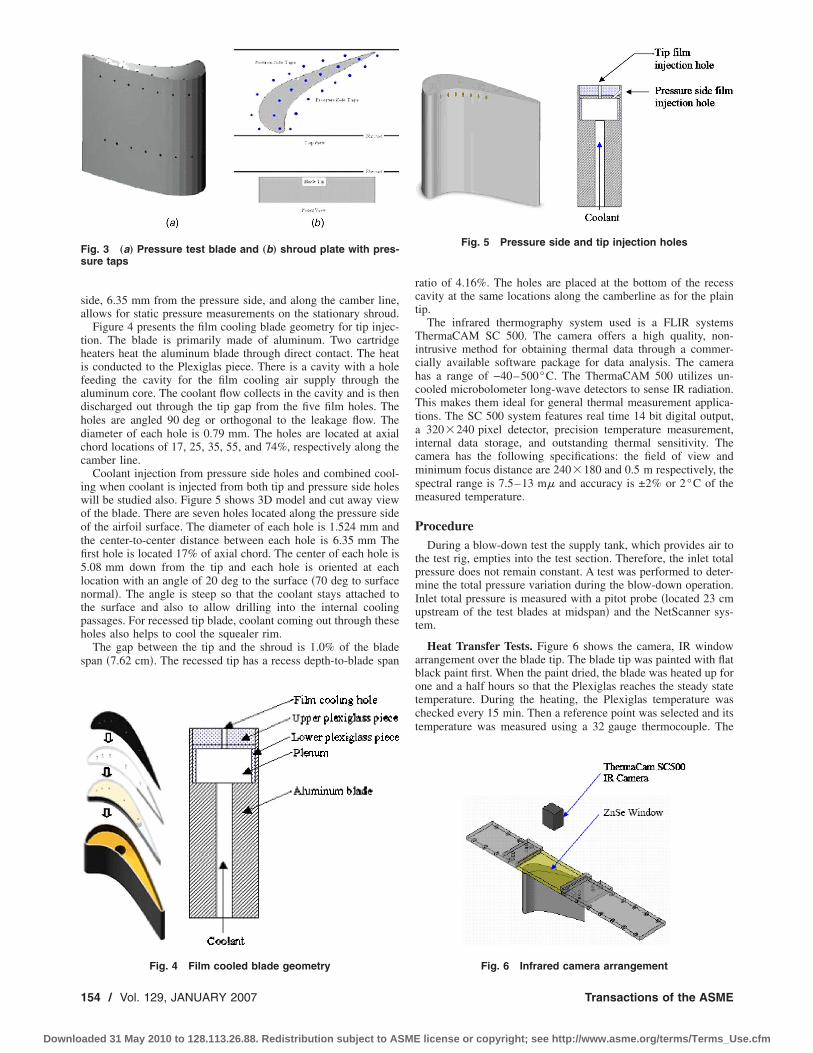
side, 6.35 mm from the pressure side, and along the camber line,allows for static pressure measurements on the stationary shroud.

Figure 4 presents the film cooling blade geometry for tip injec-tion. The blade is primarily made of aluminum. Two cartridgeheaters heat the aluminum blade through direct contact. The heatis conducted to the Plexiglas piece. There is a cavity with a holefeeding the cavity for the film cooling air supply through thealuminum core. The coolant flow collects in the cavity and is thendischarged out through the tip gap from the five film holes. Theholes are angled 90 deg or orthogonal to the leakage flow. Thediameter of each hole is 0.79 mm. The holes are located at axialchord locations of 17, 25, 35, 55, and 74%, respectively along thecamber line.

Coolant injection from pressure side holes and combined cool-ing when coolant is injected from both tip and pressure side holeswill be studied also. Figure 5 shows 3D model and cut away viewof the blade. There are seven holes located along the pressure sideof the airfoil surface. The diameter of each hole is 1.524 mm andthe center-to-center distance between each hole is 6.35 mm Thefirst hole is located 17% of axial chord. The center of each hole is5.08 mm down from the tip and each hole is oriented at eachlocation with an angle of 20 deg to the surface �70 deg to surfacenormal�. The angle is steep so that the coolant stays attached tothe surface and also to allow drilling into the internal coolingpassages. For recessed tip blade, coolant coming out through theseholes also helps to cool the squealer rim.

The gap between the tip and the shroud is 1.0% of the bladespan �7.62 cm�. The recessed tip has a recess depth-to-blade span

ratio of 4.16%. The holes are placed at the bottom of the recesscavity at the same locations along the camberline as for the plaintip.

The infrared thermography system used is a FLIR systemsThermaCAM SC 500. The camera offers a high quality, non-intrusive method for obtaining thermal data through a commer-cially available software package for data analysis. The camerahas a range of −40–500°C. The ThermaCAM 500 utilizes un-cooled microbolometer long-wave detectors to sense IR radiation.This makes them ideal for general thermal measurement applica-tions. The SC 500 system features real time 14 bit digital output,a 320�240 pixel detector, precision temperature measurement,internal data storage, and outstanding thermal sensitivity. Thecamera has the following specifications: the field of view andminimum focus distance are 240�180 and 0.5 m respectively, thespectral range is 7.5–13 m� and accuracy is ±2% or 2°C of themeasured temperature.

ProcedureDuring a blow-down test the supply tank, which provides air to

the test rig, empties into the test section. Therefore, the inlet totalpressure does not remain constant. A test was performed to deter-mine the total pressure variation during the blow-down operation.Inlet total pressure is measured with a pitot probe �located 23 cmupstream of the test blades at midspan� and the NetScanner sys-tem.

Heat Transfer Tests. Figure 6 shows the camera, IR windowarrangement over the blade tip. The blade tip was painted with flatblack paint first. When the paint dried, the blade was heated up forone and a half hours so that the Plexiglas reaches the steady statetemperature. During the heating, the Plexiglas temperature waschecked every 15 min. Then a reference point was selected and itstemperature was measured using a 32 gauge thermocouple. The

Fig. 3 „a… Pressure test blade and „b… shroud plate with pres-sure taps

Fig. 4 Film cooled blade geometry

Fig. 5 Pressure side and tip injection holes

Fig. 6 Infrared camera arrangement



thermocouple was calibrated using an ice bath and boiling waterbath. The analog/digital system was adjusted to convert the volt-age to the right temperature. This ensured a better accuracy of theresults. The IR camera is calibrated using the thermocouple placedon the surface with a high conductive aluminum tape to ensureproper contact on the surface. The tape is spray painted black toensure high emissivity. After that the emissivity was altered untilthe temperature measured by the camera agrees with the thermo-couple reading. This is the emissivity value of the reference ob-ject. However, the temperature of the reference object must not betoo close to the ambient temperature for this to work. During theemissivity calculation, zinc-selenide window was not used. So,the transmissivity value used was 1. The emissivity calibrationprovided an emissivity for the black painted surface to be 0.95.The measured transmissivity pf the zinc-selenide window foundby the calibration technique and the transmissivity value of thewindow supplied by the manufacturer matches exactly. The trans-missivity of the window is 0.75.

The heat transfer blade is coated black and is heated for 2 h toensure that its temperature reaches steady state before testing.During heating, the surface temperature is monitored by the IRcamera. The inside temperature of the Plexiglas piece is moni-tored using thermocouples. These thermocouples are checked ev-ery 5 min. Once the blade temperature reaches steady state, thecoolant flow is set to bypass and heated to about the same tem-perature as the test blade. The blade heaters are switched off, theIR camera is set to take images at periodic intervals, the coolantflow is switched into the test blade, and the pneumatic valve isthen opened so that compressed air may enter the test rig. Coolantflow temperature is measured in the cavity before the air entersthe film hole. The images are recorded and saved as data files. Thedigitized temperature values at initial condition, 5 s into the test,and 35 s into the test are provided as input into a Fortran programto calculate h and � simultaneously from Equation set �2�. Theequations are solved for every pixel location on the Plexiglas tipwhere Ti is the initial heated blade temperature before the tran-sient is initiated; Tm is the oncoming mainstream recovery tem-perature; Tc is the coolant temperature; Tw is the wall temperatureor the reference temperature during the transient test; � and k arethe thermal diffusivity and thermal conductivity of the Plexiglassurface; and t is the time at which the frames are recorded. All theabove values are either known or measured during the test and thelocal heat transfer coefficient �h� and film effectiveness �� arecalculated at every pixel location

Pressure Tests. Pressure measurements were made using aKPSI 32-channel system that acquires data at 100 Hz frequency ateach port. Static pressure measurements are made on the shroudfor each blade tip configuration. Measurements are also made onthe pressure blade suction and pressure surfaces. Before eachpressure test, moisture is blown from the pressure system dataports using the supply pressure. The data ports are calibrated andreset to zero, when necessary, to ensure accuracy. The pneumaticvalve is then opened and air enters the test rig. The duration of allpressure tests matched that of the heat transfer tests. The pressuresystem reads surface gauge static pressures. Pressure ratios arecomputed based on the measured inlet total pressure at that in-stant. Nasir et al. �1� provide more details on the test rig, basicpressure distributions for the cascade, and flow verification for thesystem.

Local Blowing Ratio Calculations. The set blowing ratio iscalled global blowing ratio because it is based on velocity of themainstream at the inlet of the cascade. But actual or local blowingratio for each hole is more than likely to be different than theglobal blowing ratio. The reason is that the amount of coolantcoming out from each hole depends on the difference betweenplenum pressure and local static pressure. If pressure difference ishigher, more coolant will come out, i.e., higher blowing ratio andvice versa. Local blowing ratio is an important parameter because

it gives us the local picture of coolant and leakage flow interac-tion. The equation used to calculate actual mass flow rate of cool-ant coming out through each hole �17� is

m = CDPtc�Pm

Ptc�� 2�

�� − 1�RTtc��Ptc

Pm��−1�/�

− 1��

4d2�

where m is the actual mass flow rate of coolant, CD is the dis-charge coefficient or the ratio of actual mass flow rate to idealmass flow rate through the film cooling hole; Ptc is the total pres-sure of coolant inside plenum; Pm is the static pressure of main-stream at the hole location based on the measured shroud pres-sures with injection; � is the specific heat ratio; R is the gasconstant; Ttc is the total temperature of coolant inside plenum; andd is the diameter of film cooling hole. The above equation as-sumes an isentropic one-dimensional expansion from the totalpressure in the coolant loop to the static pressure in the primary ormainstream. For present study, static pressure measured on thefloor of the plenum is used as the total pressure of coolant. It canbe safely assumed in our case that static and total pressures insidethe plenum are the same because plenum acts as a reservoir. Staticpressure inside the plenum is measured at two places on the floorand no significant difference in pressure readings was found. Itshows that coolant flow equalizes well inside the plenum. Thedischarge coefficient for the hole was measured with a simpleflow test and the value obtained from experiment was 0.64, 0.62,0.58 for the three blowing ratios. The value of 0.6 was used for allconditions.

Results and DiscussionThe test flow conditions at inlet to cascade were measured us-

ing hot wire anemometry. The flow inlet velocity at cascade inletwas 60 m/s, which represents a cascade inlet Mach number ofMa=0.16. The exit velocity to the cascade was 188 m/s, which isa Mach number of Ma=0.54. The Reynolds number based oncascade exit velocity and blade axial chord is 861,000. The enginecondition is simulated at entrance but the blade exit is dependenton the pressure ratio resulting in lower than engine condition ofMa=0.8. The coolant to mainstream density ratio is 0.95 and ismuch lower than the engine conditions which is typically in theorder of 1.7–2.0.

Figure 7 presents the blade pressure distribution at three differ-ent span locations for a tip gap of 1.0% of blade span plottedagainst normalized length along the pressure and suction surfaces�x /L�. The measurement locations for hub to tip are at locationsalong 33.3, 86.7, and 100% of the blade span. The local staticpressure is normalized by the cascade inlet total pressure�Ps / Po,inlet�. In the figure, curve �a� represents the pressure sideand curve �b� represents the suction side. At 33.3% blade heightfrom the hub, there is a large pressure differential between thepressure and suction surface which is the main driving potentialfor the leakage flow. Also just downstream of the leading edge,

Fig. 7 Surface pressure distributions on the blade surface andtip gap with 1% clearance gap „a… pressure surface „b… suctionsurface



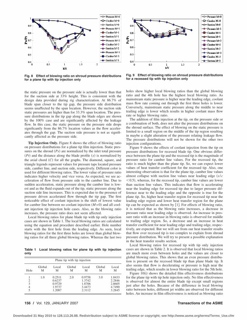
the static pressure on the pressure side is actually lower than thatfor the suction side at 33% height. This is consistent with thedesign data provided during rig characterization. At 86.7% ofblade span closer to the tip gap, the pressure side distributionseems unaffected by the span location. However, the suction sidestatic pressures are higher than for 33.3% span location. The pres-sure distributions in the tip gap along the blade edges are shownby the 100% case and are significantly affected by the leakageflow. In this case, the static pressure on the pressure side dropssignificantly from the 86.7% location values as the flow acceler-ates through the gap. The suction side pressure is not as signifi-cantly affected as the pressure side.

Tip Injection Only. Figure 8 shows the effect of blowing ratioon pressure distributions for a plane tip film injection. Static pres-sures on the shroud �Ps� are normalized by the inlet total pressure�Pt� and the distance along the blade profile �x� is normalized bythe axial chord �C� for all the graphs. The diamond, square, andtriangle legends represent values for pressure taps located pressureside, camber line, and suction side, respectively. Different color isused for different blowing ratios. The lower value of pressure ratioindicates higher velocity and vice versa. As expected, we see ac-celeration of flow from pressure side to the camber line. Due tosudden acceleration, static pressure along the camber line is low-est and as the fluid expands out of the tip, static pressure along thesuction side line increases. This is expected due to the presence ofpressure driven accelerated flow through the tip gap. The firstnoticeable effect of coolant injection is the shift of lowest valuefor camber line between no coolant injection �M =0� and all cool-ant injection tip injection hole cases. Also, as the blowing ratioincreases, the pressure ratio does not seem affected.

Local blowing ratios for plane blade tip with tip only injectioncases are shown in Table 1. The local blowing ratios are calculatedusing the equation and procedure described earlier. Hole numberstarts with the first hole from the leading edge. As seen, localblowing ratios for the first three holes are lower than global blow-ing ratios for all three global blowing ratios. Whereas the last two

holes show higher local blowing ratios than the global blowingratio and the 4th hole has the highest local blowing ratio. Asmainstream static pressure is higher near the leading edge, coolantmass flow rate coming out through the first three holes is lower.Conversely, mainstream static pressure along the middle to neartrailing edge is lower which results in higher coolant mass flowrate or higher blowing ratio.

The addition of film injection at the tip, on the pressure side ora combination of both, does not alter the pressure distributions onthe shroud surface. The effect of blowing on the static pressure islimited to a small region on the middle of the tip region resultingin maybe a slight alteration of the pressure relating leakage flow.The pressure distributions will not be shown for the other twoinjection configurations.

Figure 9 shows the effects of coolant injection from the tip onpressure distributions for recessed blade tip. One obvious differ-ence between the plane tip and the recessed tip is the magnitude ofpressure ratio for camber line values. For the recessed tip, theratio is much higher than the plane tip. So, we can expect lowervalues of heat transfer coefficient for the recessed tip. Also, oneinteresting observation is that for the plane tip, camber line valuesalmost collapse with suction line values near leading edge �x /c�0.5�, whereas, for the recessed tip, camber line values are lowerthan suction line values. This indicates that flow is acceleratingnear the leading edge for recessed tip due to larger pressure dif-ference near to the leading edge and the opposite is true for theplane tip. So, higher heat transfer region for recessed tip near theleading edge region and lower heat transfer region for the planetip can be expected as shown by �1�. For effects of blowing ratio,it is noticed that as the blowing ratio increases, a decrease inpressure ratio near leading edge is observed. An increase in pres-sure ratio with an increase in blowing ratio is observed for middleto trailing edge region. So, a decrease and an increase in heattransfer coefficient for near leading edge and trailing edge, respec-tively, are expected. But we will see from our heat transfer resultsthat flow over recessed tip is too complex to explain from shroudpressure distribution. We will try to present a possible explanationin the heat transfer results section.

Local blowing ratios for recessed tip with tip only injectioncases are shown in Table 2. It is observed that local blowing ratiosare much more even between holes and the values are closer toglobal blowing ratios. This shows that an even pressure distribu-tion is present on the recessed blade tip than plane blade tip. Italso seems that flow is decelerating or pressure is high near thetrailing edge, which results in lower blowing ratio for the 5th hole.

Figure 10�i� shows the detailed film effectiveness distributionsfor the plane tip with tip hole injection only. No film effectivenessis observed for almost the entire blade tip except small regionsjust after the holes. Because of the difference in local blowingratio between holes, different jet widths are observed for differentholes. An increase in film effectiveness is noticed as blowing ratio

Fig. 8 Effect of blowing ratio on shroud pressure distributionsfor a plane tip with tip injection only

Table 1 Local blowing ratios for plane tip with tip injectiononly

Plane tip with tip injection

HoleGlobal

MLocal

MGlobal

MLocal

MGlobal

MLocal

M

1 1.0 0.2511 2.0 0.9758 3.0 1.84332 0.6237 1.3742 2.28463 0.9729 1.8706 2.86054 1.9737 3.4473 4.74905 1.2087 2.3112 3.2845

Fig. 9 Effect of blowing ratio on shroud pressure distributionsfor a recessed tip with tip injection only



increases from 1 to 2. But a decrease in value is noticed for theblowing ratio, M =3. As seen in Table 1, the local blowing ratiosfor each hole are pretty high, which indicates high momentumjets. Due to high momentum, the coolant jet maintains a cylindri-cal structure and detaches from the injection surface and dissi-pates into the mainstream without adhering to the primary surfaceas seen for hole numbers 1 and 3. Sometimes, the jet may reattachitself to the tip surface after interacting with the opposite shroudsurface, which results in high effectiveness as seen for hole num-bers 2, 4, and 5.

Figure 10�ii� shows the detailed film effectiveness distributionsfor the squealer tip with tip hole injection only. Highest film ef-fectiveness is observed for blowing ratio, M =2. The directions ofhigh effectiveness streaks are along the camber line. The first fourholes have similar local blowing ratios and they also exhibit simi-lar film effectiveness. Interestingly, the 5th hole has lowest effec-tiveness for all three blowing ratios. It is may be due to the factthat it has the lowest local blowing ratio as noticed in Table 2. Forblowing ratio, M =3, almost no effectiveness is observed for thewhole tip. This may be due to complete detachment of the coolantjet from the injection surface.

Figure 11�i� shows the detailed heat transfer coefficient distri-butions for the plane tip with tip hole injection only. For no cool-

ant injection case �M =0�, a low heat transfer coefficient region isobserved near the leading edge. This is referred to as sweet spot.In this region, suction and camber line pressures collapse, mean-ing that there is little pressure difference to drive leakage flow.Very high heat transfer coefficient region is observed along thepressure side from middle of the blade towards trailing edge. Thisis due to the pressure side entry loss vortex. The heat transfercoefficient distribution observed is typical for plane blade tip andobserved by many previous researchers. The obvious effect ofcoolant injection is a reduction in heat transfer coefficient, espe-cially along the pressure side region. Also, horseshoe vortex isclearly visible ahead of each hole. For blowing ratio, M =1, fromthe direction of horseshoe vortex, it is clearly seen that leakageflow is directing from pressure side leading edge towards suctionside trailing edge. A region of very low heat transfer coefficientregion is also observed just after the holes. Due to acceleration offlow in between holes, higher heat transfer coefficient regions areobserved there. Due to blockage effect, heat transfer coefficientdecreases as blowing ratio increases. It is also seen that the regionof small heat transfer coefficient near the trailing region dimin-ishes as blowing ratio increases.

Figure 11�ii� shows the detailed heat transfer coefficient distri-butions for the squealer tip with tip hole injection only. Reversetrend is observed for recessed tip than plane tip. A high heattransfer coefficient region is noticed near the leading edge regionand lower values are noticed for the trailing edge region. Thisopposite trend is actually beneficial to the blade because the crosssection is the widest near the leading edge due to which it canbetter withstand higher heat load than thin trailing edge. It appearsthat as the blowing ratio increases, heat transfer coefficient de-creases, at least near the leading edge, though the decrease is notas obvious as a plane tip. Also, there is a low heat transfer regionnear the pressure side of the trailing edge region. Thickness of thisregion is smallest for the highest blowing ratio. It seems like thatfor bowing ratio, M =1 and M =2, leakage flow enters the recessedtip near the leading edge and goes out of the tip near the suctionside of the trailing edge region. For blowing ratio, M =3, possiblythe interaction between jet and leakage flow is minimum due tohigher momentum of the jet. As a result, leakage flow expandsmore and reduces the low heat transfer region.

Pressure Side Injection Only. Local blowing ratios for planetip with pressure side only coolant injection are presented in Table3. Surface pressure on the 86.7% span of the pressure side of theblade �Fig. 6� is used as reference data. So, the values presentedhere are just estimated values. The first observation is that localblowing ratio for all holes is almost equal. This is due to the factthat static pressure on the pressure surface of the blade remainsalmost constant and does not decrease sharply as compared tosuction surface. Also, local blowing ratio values are closer to glo-bal blowing ratios.

Table 4 shows local blowing ratios for recessed tip with pres-sure side injection only case. Not much of a difference is observedbetween plane and recessed blade tip cases. Though similar localblowing ratios are observed between plane and recessed blade tip,it will be observed later that heat transfer coefficient and filmeffectiveness distributions between the two blade tips are entirelydifferent. This is due to the two completely different flow patternspresent between the two blade tips.

Figure 12�i� shows the detailed film effectiveness distributionsfor the plane tip with pressure side hole injection only. Low ef-fectiveness values are observed for all blowing ratios. Coolant jetstreaks are visible for blowing ratio M =1, along the pressure side.But for blowing ratio M =2, those jet streaks are not present. Itappears that all the jets detach from the tip surface and they do notreattach themselves on the tip surface. For blowing ratio, M =3,we see the reattachment of the jets along the suction side after thejets hit the shroud surface.

Figure 12�ii� shows the detailed film effectiveness distributions

Table 2 Local blowing ratios for recessed tips with tip injec-tion only

Recessed tip with tip injection

HoleGlobal

MLocal

MGlobal

MLocal

MGlobal

MLocal

M

1 1.0 1.0953 2.0 2.0341 3.0 2.99692 1.0804 2.0758 3.08913 1.0529 2.0825 3.13054 0.9361 2.0100 3.10085 0.8567 1.7582 2.6970

Fig. 10 Detailed film effectiveness distributions with tip injec-tion only



for the recessed tip with pressure side hole injection only. No filmeffectiveness �all blue� is observed for all blowing ratios except afaint trace for blowing ratio, M =3. Overall, it appears that pres-sure side coolant injection is totally ineffective for recessed tipcase. This may be due to high pressure present inside the squealercavity. As seen in Fig. 9, pressure ratios along the camber line forrecessed tip are much higher than the plane tip. This high pressurepossibly prevents coolant jets from getting into the cavity, whichresults in no effectiveness for the recessed blade tip.

Figure 13�i� shows the detailed heat transfer coefficient distri-

butions for the plane tip with pressure side hole injection only.One obvious effect of pressure side coolant injection is the reduc-tion in heat transfer coefficient along the pressure side that isobserved for no injection or M =0 case. It appears that separationentry vortices are no longer present for all the coolant injectioncases. It has also been noticed that high heat transfer coefficientregions are present along the suction side for blowing ratio M=1 case. These regions diminish as blowing ratio increases to 2.The high heat transfer coefficient regions for blowing ratio M

Fig. 11 Detailed heat transfer coefficient distributions with tip injection only

Table 3 Local blowing ratios for plane tip with pressure sideinjection

Plane tip with pressure side injection

HoleGlobal

MLocal

MGlobal

MLocal

MGlobal

MLocal

M

1 1.0 1.0462 2.0 2.0573 3.0 3.05172 0.9691 1.9513 2.95443 0.9803 1.9666 2.96844 0.9900 1.9799 2.98055 0.9870 1.9758 2.97676 1.0013 19953 2.99457 1.0314 2.0368 3.0328

Table 4 Local blowing ratios for recessed tip with pressureside injection

Recessed tip with pressure side injection

HoleGlobal

MLocal

MGlobal

MLocal

MGlobal

MLocal

M

1 1.0 1.0307 2.0 2.0527 3.0 3.04842 0.9666 1.9662 2.96883 0.9759 1.9785 2.98024 0.9839 1.9894 2.99005 0.9814 1.9860 2.98706 0.9933 2.0019 3.00167 1.0184 2.0359 3.0329



=3 are due to reattachment of coolant jets along the suction sideregion of the tip surface. Also, streaks of jets marked by low heattransfer regions are visible along the pressure side of the blade tip.

Figure 13�ii� shows the detailed heat transfer coefficient distri-butions for the recessed tip with pressure side hole injection only.No injection case and blowing ratio M =1 cases are almost iden-tical except the low heat transfer coefficient region located nearthe pressure side trailing edge for M =1 case. This low heat trans-fer region is present for all blowing ratio cases. As blowing ratioincreases, the high heat transfer coefficient region near the leadingedge continues to decrease in size.

Combined Pressure Side and Tip Hole Injection. Localblowing ratios for plane tip with combination injection cases areshown in Table 5. It is observed that local blowing ratios for tipcoolant holes are higher than pressure side holes. In fact, localblowing ratios for tip coolant holes are higher than global blowingratios. This is due to the fact that pressure side surface has higherpressure than blade tip especially the camber line where the tipcoolant holes are located. This high pressure is causing less cool-ant to come out through the pressure side holes in comparison tothe tip holes. Again, the 4th tip hole has the highest value. If localblowing ratios for tip holes in Table 1 �tip only injection� arecompared to local blowing ratios for tip holes in Table 5 �combi-nation injection�, a significant increase in local blowing ratios forcombination cases is observed for all the holes, especially for thefirst hole. As will be seen later, this increase in blowing ratio fortip holes causes substantial impact between coolant and main-stream interaction, particularly for blowing ratio, M =3.0.

Local blowing ratios for recessed tip with combination coolantinjection are shown in Table 6. Again, tip holes have higher localblowing ratios than pressure side holes. But the tip holes for re-cessed tip have lower local blowing ratios than plane tip and theopposite is true for pressure side holes. This is due to higher staticpressure on the recessed blade tip than plane tip. Also, the tipholes have almost equal local blowing ratios and the values arehigher than global blowing ratios.

Figure 14�i� shows the effect of blowing ratio on detailed filmeffectiveness for plane tip pressure distribution for combined

coolant injection. For blowing ratio, M =1 and M =2, coolant jetsare much wider than tip only and pressure side injection onlycases. This is obviously due to the combined injection and higherblowing ratios. Also, small effectiveness values are observed inbetween holes because of the injection from pressure side holes.For blowing ratio, M =3, high film effectiveness value of around0.5 is observed for holes 2, 4, and 5. It appears that for a highblowing ratio of M =3, coolant jet from the tip hits the shroud firstand then adheres back onto the blade tip resulting in higher filmeffectiveness. This was not observed for tip only and pressure sideinjection only cases because in combination cases the pressureside injection jets are creating a barrier for the tip injection jets. Inaddition, the tip holes have higher blowing ratios and this highermomentum of the jets causes minimum interaction between leak-age flow and tip injection jet. As a result, the tip jets shoot up andthen reattach back onto the tip. Also, some reattachments of pres-sure side injection jets are observed for this case. High effective-ness values are observed in regions between holes. This is due tothe reattachments of jets coming out of the pressure side holes.

Figure 14�ii� presents the effect of blowing ratio on detailedfilm effectiveness distributions for combined injection on a re-cessed tip. Blowing ratio, M =1 and M =2, shows the almost samelevel of effectiveness. The high effectiveness regions are aroundholes 2, and 3. Though all the tip holes have similar local blowingratios, holes 1, 3, and 5 are not showing lesser effectiveness. Thisis possibly due to the fact that effectiveness not only depends onlocal blowing ratios but also it depends on how the jet is interact-ing with leakage flow locally. It appears that leakage flow ispushed along the camber line from the leading edge towards thetrailing edge and does not cross from pressure side to suction sideas is the case without film injection. As expected, high film effec-tiveness values are observed for blowing ratio, M =3 case. But thelevel of effectiveness is lower than the plane tip case.

Ahn et al. �5� also shows similar film effectiveness results for adifferent blade where they considered tip and pressure side injec-tion. They also showed film effectiveness distributions on thepressure side edge where coolant is injected. However, the levelsof film effectiveness obtained in this study and their study are ingood correlation. The main focus of the present study is to indi-cate the effects for a different blade with different pressure distri-butions are similar. However, locally, the effects are clearly de-pendent on the pressure distributions that drive the tip leakageflow.

Figure 15�i� shows the effect of blowing ratio on detailed heattransfer coefficient distributions for plane tip with combined cool-ant injection. Coolant injection decreases the heat transfer coeffi-cient compared to the no injection case. For blowing ratio, M =2,streaks of jets from pressure side holes are visible along the pres-sure side of the blade. These streaks are not visible for the blow-ing ratio 1 case. For blowing ratio, M =3, very high heat transfercoefficient regions are observed around holes 2, 4, and 5. Thesebutterfly-shaped regions are extended from the middle of theblade towards the suction side. It appears that for this high blow-ing ratio, coolant jet from the tip hits the shroud first and thenbounces back onto the blade tip. This was not observed for tiponly and pressure side injection only cases because in combina-tion cases, the pressure side injection jets are creating a barrier forthe tip injection jets. In addition, the tip holes have higher blowingratios and this higher momentum of the jets causes minimum in-teraction between leakage flow and tip injection jet. As a result,the tip jets shoot up and then reattach back on to the tip. Also,some reattachments of pressure side injection jets are observed forthis case.

Figure 15�ii� presents the effect of blowing ratio on detailedheat transfer coefficient distributions for combined injection on arecessed tip. It has been observed that the high heat transfer co-efficient region that is present in no injection case is absent forblowing ratio, M =1 case. For tip only and pressure side injectiononly cases, this high heat transfer coefficient region was present

Fig. 12 Detailed film effectiveness distributions with pressureside injection only



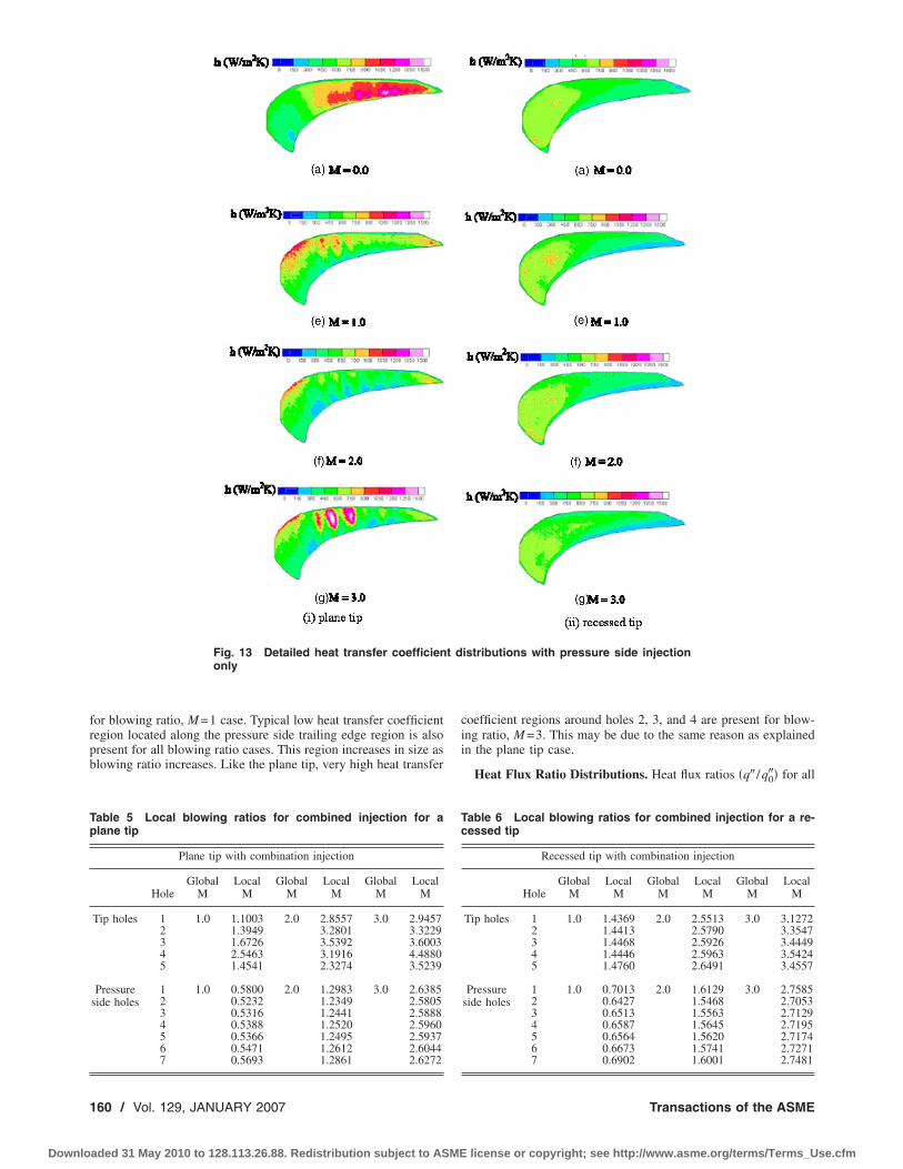
for blowing ratio, M =1 case. Typical low heat transfer coefficientregion located along the pressure side trailing edge region is alsopresent for all blowing ratio cases. This region increases in size asblowing ratio increases. Like the plane tip, very high heat transfer

coefficient regions around holes 2, 3, and 4 are present for blow-ing ratio, M =3. This may be due to the same reason as explainedin the plane tip case.

Heat Flux Ratio Distributions. Heat flux ratios �q� /q0�� for all

Fig. 13 Detailed heat transfer coefficient distributions with pressure side injectiononly

Table 5 Local blowing ratios for combined injection for aplane tip

Plane tip with combination injection

HoleGlobal

MLocal

MGlobal

MLocal

MGlobal

MLocal

M

Tip holes 1 1.0 1.1003 2.0 2.8557 3.0 2.94572 1.3949 3.2801 3.32293 1.6726 3.5392 3.60034 2.5463 3.1916 4.48805 1.4541 2.3274 3.5239

Pressureside holes

1 1.0 0.5800 2.0 1.2983 3.0 2.63852 0.5232 1.2349 2.58053 0.5316 1.2441 2.58884 0.5388 1.2520 2.59605 0.5366 1.2495 2.59376 0.5471 1.2612 2.60447 0.5693 1.2861 2.6272

Table 6 Local blowing ratios for combined injection for a re-cessed tip

Recessed tip with combination injection

HoleGlobal

MLocal

MGlobal

MLocal

MGlobal

MLocal

M

Tip holes 1 1.0 1.4369 2.0 2.5513 3.0 3.12722 1.4413 2.5790 3.35473 1.4468 2.5926 3.44494 1.4446 2.5963 3.54245 1.4760 2.6491 3.4557

Pressureside holes

1 1.0 0.7013 2.0 1.6129 3.0 2.75852 0.6427 1.5468 2.70533 0.6513 1.5563 2.71294 0.6587 1.5645 2.71955 0.6564 1.5620 2.71746 0.6673 1.5741 2.72717 0.6902 1.6001 2.7481



the cases takes into account the effect of both heat transfer coef-ficient and film effectiveness values. The heat flux ratio is calcu-lated based on the formulation presented by Mehendale et al. �18�.The heat transfer ratio with and without film injection �h /h0� andthe local film effectiveness are used to calculate the local heat fluxratio.

q�

q0�=

h

h0�1 −

�

�

The term is the overall cooling effectiveness and ranges be-tween 0.5 and 0.7 for typical blade cooling systems. In this study,a typical value of 0.6 is chosen. The areas where the ratio is lessthan one show benefit from film cooling.

Figure 16 shows the detailed heat flux ratios on a plane andrecessed tip with tip injection only. This takes into account thecombined effect of film effectiveness and heat transfer coefficient.For plane tip cases, a decrease in net heat flux ratio value forentire tip is observed as blowing ratio increases. Values of morethan 1 are observed near the leading edge region. This is due tothe fact that, the no-coolant case has a very low heat transfercoefficient region, whereas coolant injection actually increasesheat transfer coefficient in that region and film effectiveness val-ues are not high enough to make up for the increase in heat trans-fer coefficient. Also, just after the holes, very low values are ob-served. This is because of high film effectiveness and low heattransfer coefficient values. Also, a thin region of higher net fluxratio region is observed along the suction side region. For re-cessed tip blade, as blowing ratio increases from 1 to 2, we see adecrease in net heat flux ratio values. The high value region nearthe leading edge for blowing ratio, M =1, is due to the high heattransfer region observed in the detailed heat transfer coefficientdistributions in Fig. 11. For blowing ratio, M =3, small areas ofhigh neat flux ratio are observed near the trailing edge. They arelocated along the jet direction. It seems that the jet increased theheat transfer coefficient in those areas without producing anycooling effectiveness.

Figure 17 shows the detailed heat flux ratios on a plane andsquealer tip with pressure side injection only. For plane tip cases,

a high value region is observed near the leading edge. The valuedecreases as blowing ratio increases. It appears that pressure sidecoolant injection redirected the leakage flow for the plane tip.Low value regions can be seen along the pressure side. This is adirect effect of the coolant jets. For recessed tip blade, the value ofnet heat flux ratio is close to 1 for almost all the tip region. Thisindicates that pressure side coolant injection for the recessed tipblade is not beneficial at least for the tip. It may, however, help incooling the thin squealer rim.

Figure 18 shows the detailed heat flux ratios on a plane andsquealer tip with combined tip and pressure side injection. For theplane tip, the values are lower than 1 for most of the blade tip.Blowing ratio, M =2, shows low net heat flux ratio regions alongpressure side of the blade tip. A small high value region nearleading edge is observed for blowing ratio, M =3. Recessed tipshows even distribution of net heat flux ratio except a few smallareas for blowing ratio, M =1 and M =2. For blowing ratio 3, thehigh value region is present near leading edge, which extends tothe middle of the blade.

ConclusionsDetailed film effectiveness measurements were made on a high

pressure turbine blade tip with an inlet total-to-outlet static pres-sure ratio of 1.2. A transient infrared thermography technique wasused to obtain both heat transfer coefficient and film effectivenessin a single test. The heat transfer coefficients and heat flux reduc-tion analysis are presented in the companion paper. The effects ofcoolant injection on plane and recessed blade tip were studied forblowing ratios of M =1.0, 2.0, and 3.0. Three cases studied for thiscase were: �1� coolant injection from holes located on the bladetip, �2� coolant injection from holes located near the tip along thepressure side and, �3� combination cases when coolant is injectedboth from tip holes and pressure side holes. For tip injectioncases, it was found that as blowing ratio increases, film effective-ness changed slightly for both plane and recessed tip blade. Also,at highest blowing ratio, lift-off of jets is observed for both bladetips. Injection of coolant from pressure side holes was found to beless effective than tip injection. It appears to be good for plane tipin reducing heat load along the pressure side. But no film effec-tiveness is observed for the recessed tip case. Combined coolingwas found to be the best among the three cases. For this case, ahigh value of film effectiveness is observed for most of the bladetip. It is observed that local blowing ratio is an important param-eter to understand flow behavior and, particularly for plane tip,local blowing ratios are much more different than global blowingratios.

For tip injection cases, it was found that as blowing ratio in-creases, heat transfer coefficient decreases for both plane and re-cessed tip blade. Also, at highest blowing ratio, lift-off of jets isobserved for both blade tips. Injection of coolant from pressureside holes was found to be less effective than tip injection. Itappears to be good for plane tip in reducing heat load along thepressure side. At highest blowing ratio, M =3, very high values ofheat transfer coefficient are observed. It appears that for this highblowing ratio, coolant jet from the tip hits the shroud first and thenbounces back onto the blade tip. It is observed that local blowingratio is an important parameter to understand flow behavior and,particularly for plane tip, local blowing ratios are much moredifferent than global blowing ratios. Overall, high blowing ratiosproduce high heat flux ratios resulting in increased heat transferon the tip surface for squealer tips.

Overall, it appears that the pressure side injection reduces leak-age flow into the tip gap and helps improve protection of the tipsurface with the tip injection. However, pressure side injectionmay also protect the pressure side edge of the tip surface which isprone to erosion. This study did not have any results on the pres-sure side and suction side edges. For recessed tips, pressure sideinjection may also help protect the rim of the squealer cavity.

Fig. 14 Detailed film effectiveness distributions with com-bined injection



Fig. 16 Detailed heat flux ratio distributions for plane andsquealer tips with tip injection only

Fig. 17 Detailed heat flux ratio distributions for plane andsquealer tips with pressure side injection only

Fig. 15 Detailed heat transfer coefficient distributions with combined injection



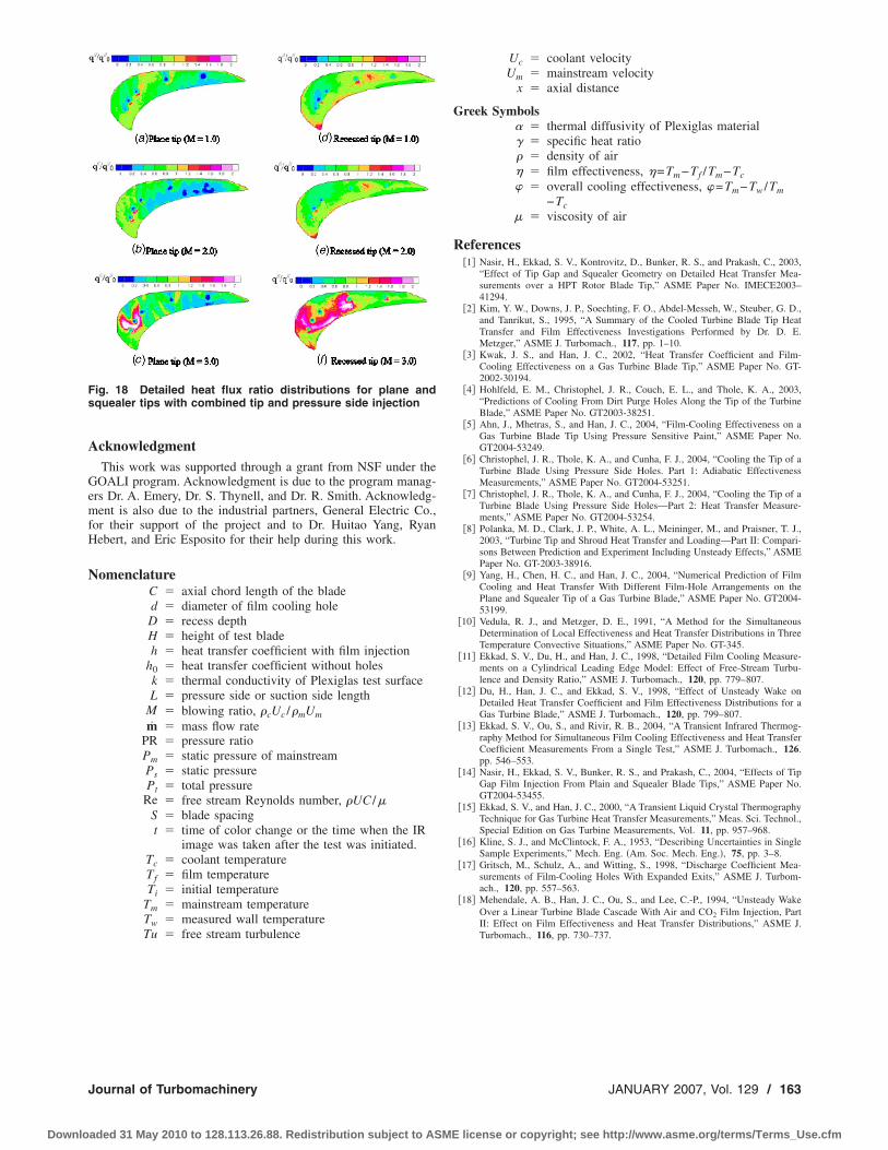
AcknowledgmentThis work was supported through a grant from NSF under the

GOALI program. Acknowledgment is due to the program manag-ers Dr. A. Emery, Dr. S. Thynell, and Dr. R. Smith. Acknowledg-ment is also due to the industrial partners, General Electric Co.,for their support of the project and to Dr. Huitao Yang, RyanHebert, and Eric Esposito for their help during this work.

NomenclatureC axial chord length of the bladed diameter of film cooling holeD recess depthH height of test bladeh heat transfer coefficient with film injection

h0 heat transfer coefficient without holesk thermal conductivity of Plexiglas test surfaceL pressure side or suction side length

M blowing ratio, �cUc /�mUmm mass flow rate

PR pressure ratioPm static pressure of mainstreamPs static pressurePt total pressure

Re free stream Reynolds number, �UC /�S blade spacingt time of color change or the time when the IR

image was taken after the test was initiated.Tc coolant temperatureTf film temperatureTi initial temperature

Tm mainstream temperatureTw measured wall temperatureTu free stream turbulence

Uc coolant velocityUm mainstream velocity

x axial distance

Greek Symbols� thermal diffusivity of Plexiglas material� specific heat ratio� density of air� film effectiveness, �=Tm−Tf /Tm−Tc� overall cooling effectiveness, �=Tm−Tw /Tm

−Tc� viscosity of air

References�1� Nasir, H., Ekkad, S. V., Kontrovitz, D., Bunker, R. S., and Prakash, C., 2003,

“Effect of Tip Gap and Squealer Geometry on Detailed Heat Transfer Mea-surements over a HPT Rotor Blade Tip,” ASME Paper No. IMECE2003–41294.

�2� Kim, Y. W., Downs, J. P., Soechting, F. O., Abdel-Messeh, W., Steuber, G. D.,and Tanrikut, S., 1995, “A Summary of the Cooled Turbine Blade Tip HeatTransfer and Film Effectiveness Investigations Performed by Dr. D. E.Metzger,” ASME J. Turbomach., 117, pp. 1–10.

�3� Kwak, J. S., and Han, J. C., 2002, “Heat Transfer Coefficient and Film-Cooling Effectiveness on a Gas Turbine Blade Tip,” ASME Paper No. GT-2002-30194.

�4� Hohlfeld, E. M., Christophel, J. R., Couch, E. L., and Thole, K. A., 2003,“Predictions of Cooling From Dirt Purge Holes Along the Tip of the TurbineBlade,” ASME Paper No. GT2003-38251.

�5� Ahn, J., Mhetras, S., and Han, J. C., 2004, “Film-Cooling Effectiveness on aGas Turbine Blade Tip Using Pressure Sensitive Paint,” ASME Paper No.GT2004-53249.

�6� Christophel, J. R., Thole, K. A., and Cunha, F. J., 2004, “Cooling the Tip of aTurbine Blade Using Pressure Side Holes. Part 1: Adiabatic EffectivenessMeasurements,” ASME Paper No. GT2004-53251.

�7� Christophel, J. R., Thole, K. A., and Cunha, F. J., 2004, “Cooling the Tip of aTurbine Blade Using Pressure Side Holes—Part 2: Heat Transfer Measure-ments,” ASME Paper No. GT2004-53254.

�8� Polanka, M. D., Clark, J. P., White, A. L., Meininger, M., and Praisner, T. J.,2003, “Turbine Tip and Shroud Heat Transfer and Loading—Part II: Compari-sons Between Prediction and Experiment Including Unsteady Effects,” ASMEPaper No. GT-2003-38916.

�9� Yang, H., Chen, H. C., and Han, J. C., 2004, “Numerical Prediction of FilmCooling and Heat Transfer With Different Film-Hole Arrangements on thePlane and Squealer Tip of a Gas Turbine Blade,” ASME Paper No. GT2004-53199.

�10� Vedula, R. J., and Metzger, D. E., 1991, “A Method for the SimultaneousDetermination of Local Effectiveness and Heat Transfer Distributions in ThreeTemperature Convective Situations,” ASME Paper No. GT-345.

�11� Ekkad, S. V., Du, H., and Han, J. C., 1998, “Detailed Film Cooling Measure-ments on a Cylindrical Leading Edge Model: Effect of Free-Stream Turbu-lence and Density Ratio,” ASME J. Turbomach., 120, pp. 779–807.

�12� Du, H., Han, J. C., and Ekkad, S. V., 1998, “Effect of Unsteady Wake onDetailed Heat Transfer Coefficient and Film Effectiveness Distributions for aGas Turbine Blade,” ASME J. Turbomach., 120, pp. 799–807.

�13� Ekkad, S. V., Ou, S., and Rivir, R. B., 2004, “A Transient Infrared Thermog-raphy Method for Simultaneous Film Cooling Effectiveness and Heat TransferCoefficient Measurements From a Single Test,” ASME J. Turbomach., 126.pp. 546–553.

�14� Nasir, H., Ekkad, S. V., Bunker, R. S., and Prakash, C., 2004, “Effects of TipGap Film Injection From Plain and Squealer Blade Tips,” ASME Paper No.GT2004-53455.

�15� Ekkad, S. V., and Han, J. C., 2000, “A Transient Liquid Crystal ThermographyTechnique for Gas Turbine Heat Transfer Measurements,” Meas. Sci. Technol.,Special Edition on Gas Turbine Measurements, Vol. 11, pp. 957–968.

�16� Kline, S. J., and McClintock, F. A., 1953, “Describing Uncertainties in SingleSample Experiments,” Mech. Eng. �Am. Soc. Mech. Eng.�, 75, pp. 3–8.

�17� Gritsch, M., Schulz, A., and Witting, S., 1998, “Discharge Coefficient Mea-surements of Film-Cooling Holes With Expanded Exits,” ASME J. Turbom-ach., 120, pp. 557–563.

�18� Mehendale, A. B., Han, J. C., Ou, S., and Lee, C.-P., 1994, “Unsteady WakeOver a Linear Turbine Blade Cascade With Air and CO2 Film Injection, PartII: Effect on Film Effectiveness and Heat Transfer Distributions,” ASME J.Turbomach., 116, pp. 730–737.

Fig. 18 Detailed heat flux ratio distributions for plane andsquealer tips with combined tip and pressure side injection



A. Pfau

A. I. Kalfas

R. S. Abhari

Turbomachinery Laboratory,Swiss Federal Institute of Technology,

8092 Zurich, Switzerland

Making Use of LabyrinthInteraction FlowIt is the aim of this publication to attract the designers attention to the end wall flowinteractions of shrouded high pressure turbines. One of the key issues for designing betterturbines is the understanding of the flow interactions set up by the presence of labyrinthseals. Those interaction flows are carefully examined in this publication using the controlvolume analysis and the radial equilibrium of forces acting on streamlines. The conse-quences on secondary flow development and mixing losses are discussed and quantified.Out of this insight, design recommendations are derived, which attempt to make use ofthe nature of the labyrinth interaction flow. The open labyrinth cavities are classified in asystematic way. The aim of this approach is to work out the characteristic differencesbetween hub and tip cavities and those having a leakage jet or sucking main flow fluidinto the labyrinth. The influence on the main flow is discussed in terms of the incidenceflow angle of downstream blade rows and the associated loss production mechanisms.The design strategies presented in this paper follow two paths: (a) Optimization of themixing losses of the leakage jets at hub and tip is estimated to result in an efficiencyincrease of up to 0.2%. (b) The nonaxisymmetric shaping of the labyrinth interaction flowpath aims at the secondary flow control in downstream blade rows. This approach mightcontribute in the same magnitude of order as reduction in the mixing losses.�DOI: 10.1115/1.2218571�

IntroductionLabyrinth leakage flow in shrouded turbines is looked upon as

an inherently detrimental effect and something which the designercannot avoid. One design recommendation is to minimize theleakage flow through designing better labyrinth seals and to re-duce the gap widths as much as possible. If heat transfer is anissue as in a gas turbine the gap must allow enough leakage massflow in order to cool the turbine shrouds. The inlet to a labyrinthand the exit including the leakage jet alter the flow field in turbineend wall regions. This is of special significance in low aspect ratioturbine stages where secondary flows are strong. The labyrinthseal can be optimized for itself including mechanical limits andthrough flow coefficients.

The subject of cavity interactions in turbines was initially ad-dressed by Denton and Johnson �1�. However, it is only in recentyears that this subject attracted the attention of the turbomachin-ery research community. Peters et al. �2� examined the effect ofgap size on the steady interaction between the leakage flow andthe secondary flow field of a subsequent stator in a 1.5 stage,shrouded axial turbine. Hunter and Manwaring �3� reported abouttwo extra vortices generated in a downstream stator blade row.Wallis et al. �4� observed that strong interactions are present inopen cavities of shrouded turbine blades. The following bladerows were found to receive the tip flow at a negative incidence.Cao et al. �5� report about an unsteady, incompressible flow phe-nomenon affecting the interaction between the rim seal and mainannulus flows and not being related to the blade passing fre-quency. Anker and Mayer �6� numerically investigated the leakageinteraction with the main flow and found that the tip leakage flowis not uniform in the pitch-wise direction. Schlienger et al. �7�changed the geometry of the labyrinth exit cavities by introducinginserts and compared the effects on the main flow as well as onthe efficiency. These studies have focused mainly on the interac-tion occurring in the main flow and following blade passages.

However, as the origins of these interactions are open cavities,an increased emphasis should be placed on the associated steadyand unsteady flow interactions within these cavities. From theseconsiderations the question arises: Is there any potential in im-proving the overall performance of low aspect ratio, shroudedturbines by looking at the combined system of main flow duct andlabyrinth seal? In that respect, the present publication attempts toconclusively summarize and complete the work which already hasbeen published in �8,9�. It is the aim of this publication to give anoverview of labyrinth interaction effects occurring in shroudedturbines with large inlet and exit cavities. Additionally, all opencavities are treated in a systematic way and effects on the mainflow are discussed and quantified. Based on the detailed flow un-derstanding, which was experimentally gained in a two stage,shrouded, low speed turbine, new design features are derived for arange of open cavities. With this step, design modifications areproposed, which actually make use of the labyrinth interactionflows.

Test Rig, Measurement Technology, and Data SetThe cavity interaction flow was investigated in the two-stage

low speed axial turbine “LISA.” The test rig is described in detailin Sell et al. �10�. The main characteristics of the turbine aresummarized in Table 1.

The constant annulus of the turbine and the four blade rows aredepicted in Fig. 1. The stepped shrouds on the blades togetherwith three sealing fins form the labyrinth seal. The geometry un-der investigation is similar to steam turbine applications, wherelarge inlet and exit cavities allow for axial displacement of therotor shaft due to thermal expansion of the rotor. Consequently,the blade profiles are of a medium loaded type with 50% reactionand leaned stator blades. The cylindrical coordinate system usedin this publication is indicated in Fig. 1. The results are presentedlooking upstream as the observer indicates. The cavities are num-bered for an easier identification in later discussions.

The measurement technology applied was a miniature five-holeprobe of 0.9 mm head diameter and a virtual four sensor probe of0.84 mm head diameter. The accuracy of the five-hole probe read-ings is discussed in detail in �11�. The corresponding error bars are




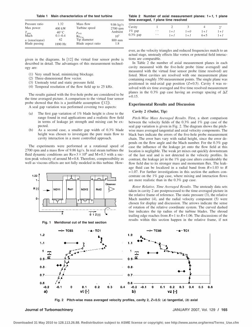
given in the diagrams. In �12� the virtual four sensor probe isdescribed in detail. The advantages of this measurement technol-ogy are:

�1� Very small head, minimizing blockage.�2� Three-dimensional flow vector.�3� Unsteady total and static pressure field.�4� Temporal resolution of the flow field up to 25 kHz.

The results gained with the five-hole probe are considered to bethe time averaged picture. A comparison to the virtual four sensorprobe showed that this is a justifiable assumption ��12��.

A seal gap variation was performed covering two aspects:

�a� The first gap variation of 1% blade height is close to therange found in real applications and a realistic flow fieldin terms of leakage jet strength and mixing can be ex-pected.

�b� As a second case, a smaller gap width of 0.3% bladeheight was chosen to investigate the pure main flow tocavity interaction in a more controlled approach.

The experiments were performed at a rotational speed of2700 rpm and a mass flow of 9.86 kg/s. In real steam turbines thefluid dynamic conditions are Re=3�106 and M=0.3 with a suc-tion peak velocity of around M=0.8. Therefore, compressibility aswell as viscous effects are not fully modeled in this turbine. How-

ever, as the velocity triangles and reduced frequencies match to anactual stage, unsteady effects like vortex or potential field interac-tions are comparable.

In Table 2 the number of axial measurement planes in eachcavity measured with the five-hole probe �time averaged� andmeasured with the virtual four sensor probe �time resolved� arelisted. Most cavities are resolved with one measurement planecontaining roughly 350 measurement points. The single plane waspositioned in mid-axial gap position �Z=0.5�. Cavity 4 was re-solved with six time averaged and five time resolved measurementplanes in the 0.3% gap case having an average spacing of �Z=0.15.

Experimental Results and Discussion

Cavity 2 (Outlet, Tip)

Pitch-Wise Mass Averaged Results. First, a short comparisonbetween the velocity fields of the 0.3% and 1% gap case of theseal gap variation is given in Fig. 2. The diagram shows the pitch-wise mass averaged tangential and axial velocity components. Theblack bars indicate the errors of the five-hole probe measurementchain. The error bars vary with radial height, since the error de-pends on the flow angle and the Mach number. For the 0.3% gapcase the influence of the leakage jet onto the flow field at thislocation is negligible. The weak jet mixes out quickly downstreamof the last seal and is not detected in the velocity profiles. Incontrast, the leakage jet in the 1% gap case alters considerably theflow field due to its stronger mass and momentum flux. The leak-age fluid can be localized in a radial band from R=1.03 to R=1.07. For further investigations in this section the authors con-centrate on the 1% gap case, where mixing and interaction flowsare more realistic than in the 0.3% gap case.

Rotor Relative, Time Averaged Results. The unsteady data setstaken in cavity 2 are postprocessed to the time-averaged picture inthe relative frame of reference. The static pressure �3�, the relativeMach number �4�, and the radial velocity component �5� werechosen for display and discussion. The arrows indicate the senseof rotation of the relative coordinate system. The curved dashedline indicates the tip radius of the turbine blades. The shroudtrailing edge reaches from R=1 to R=1.06. The discussions of theresults within this section happen in the relative frame, if not

Table 2 Number of axial measurement planes: 1+1, 1 planetime averaged, 1 plane time resolved

Cavity 1 2 3 4 2�1% gap ¯ 1+1 1+0 1+1 1+10.3% gap ¯ 1+1 1+1 6+5 1+1

Fig. 1 Meridional cut of the test section

Table 1 Main characteristics of the test turbine

Pressure ratio 1.32 Mass flow 9.86 kg/sMax power 400 kW Turbine speed 2700 rpmTinlet 40°C pexit

AmbientMach 0.1–0.4 ReCax 105

n �rotor/stator� 42 Tip diameter 800 mmBlade passing 1890 Hz Blade aspect ratio 1.8

Fig. 2 Pitch-wise mass averaged velocity profiles, cavity 2, Z=0.5: „a… tangential, „b… axial



stated otherwise.The static pressure distribution �Fig. 3� reveals the trailing edge

position of the rotor blade at �rel=−0.3 �dashed line�, where ahigh static pressure is induced. The circumferential pressure varia-tion from high to low pressure at �rel=0.3 in the main flow regionis also seen in the cavity. A stripe of higher static pressure at theradial position of the leakage jet �R=1.06� is found. The circum-ferential variation at R=1.06 is such that a low pressure regionoccurs at �rel=0.38. In addition, the level of static pressure withinthe cavity is on average �Cps=0.01 higher than in the main flow.The circumferential static pressure distribution is imposed ontothe cavity flow by the blade to blade pressure field.

The Mrel distribution �Fig. 4� shows the rotor wake at �rel=0.05 �dash-dotted line�. The wake is convected into tangentialdirection by ��rel=0.35 from the location of the trailing edge. Onthe pressure side of the wake, a higher Mrel is detected than on thesuction side. Assuming a constant relative total pressure of therotor exit flow, this effect is induced by the static pressure field.

Closer to the tip radius the wake becomes wider. A band oflower Mrel is found between R=1.03 and R=1.07, which corre-sponds to the leakage jet position observed in Fig. 2. In a regionhaving its center at �rel=0.2 and R=1.05, Mrel reaches a localminimum of 0.24. The relative total pressure in the cavity is set upby the leakage jet and distributed such that the local minimum invelocity is found on the pressure side of the rotor wake. For thiscircumferential distribution of the leakage fluid two reasons canbe provided: first, the momentum and kinetic energy distributionof the leakage jet at the exit of the last seal and, second, the staticpressure field set up by the flow field in the main annulus includ-ing the trailing edge pressure field.

Discussing the radial velocity component given in Fig. 5, addi-tional details of the leakage interaction are found. The rotor wake

is indicated with the dashed line. The regions of large negativeradial velocities vr=−0.15 �red� are not considered for discussion.The reason for this is the fact that the error in the results for thevirtual four sensor probe rapidly rises for absolute Mach numberslower than 0.06. The gray shaded symbols at R=1 indicate a bandof radial positions where the absolute Mach number falls from 0.1to below 0.06. This deficit of absolute velocity corresponds to thewake of the shroud. The radial velocity is negative within theregion of the leakage jet �R=1.06� having a minimum radial ve-locity of vr=−0.09 at the circumferential position of the wake.This value is of the same order of magnitude as the radial velocitywithin the wake itself �vr=−0.08�. The leakage fluid moves out ofthe cavity mainly below the wake position, filling up the area oflower relative kinetic energy of the wake.

Leakage to Main Flow Interaction. The basic components ofthe leakage jet to main flow interaction found in the 1% gap casein cavity 2 comprise three points:

�1� Leakage fluid migrates into the rotor wake causing theleakage streamlines to contract into the wake area. The ra-dial migration of the leakage fluid leads to a broadening ofthe wake in the vicinity of the blade tip. The wake seems toattract low kinetic energy fluid.

�2� The potential field of the rotor trailing edge divides theleakage sheet into distinct jets. Figure 6�a� shows the timeaveraged relative velocity triangles within the relativeframe of reference for the first rotor exit flow field �cavity2�. It represents the velocity vectors found with two cuts in4, one at R=0.91 and the other at R=1.06. The upper vec-tors represent the leakage jet �R=1.06� and the lower onethe main flow at R=0.91. Note that the base of the velocityvector is representing the location of the circumferentialcoordinate. The arrow represents 100% of the shroud rimspeed. The circles point out the base of velocity vectors,which are facing the trailing edge position of the rotor�rel=−0.25. The leakage mass flow is redistributed from ahomogeneous distribution within the last gap. A maximumof leakage mass flow is found in the mid position betweenthe trailing edges where it forms a distinct jet �see the dot-ted ellipse�. The main flow is much less affected by thetrailing edge pressure field than the leakage jet. The mainflow vectors reveal the wake of the rotor blade.

�3� The potential field of the stator leading edge three-dimensionally redistributes the flow field in the absoluteframe of reference. This effect is visualized in Fig. 6�b�,which presents the circumferential distribution of the abso-lute velocity triangles in the stator frame of reference forthe 1% gap case. The diagram depicts the velocity vectorsof the leakage fluid in the upper part and the velocity vec-tors of the main flow at R=0.9 in the lower part. The ve-

Fig. 3 Nondimensional static pressure Cpstime averaged, ro-

tor relative frame, Z=0.5

Fig. 4 Relative Mach number Mrel, time averaged, rotor relativeframe; Z=0.5

Fig. 5 Nondimensional radial velocity component, time aver-aged, rotor relative frame, Z=0.5



locity arrow represents 20% of the shroud rotational speed.The leading edge position of the stator is obvious in thedownstream flow field of the first rotor �cavity 2�, where itcauses a deviation of streamlines. The circles point out the

base of velocity vectors, which are facing the leading edgeposition of the stator at �rel=−0.22. Downstream of thesecond rotor �cavity 2�� this effect is not present and thevelocity vectors of the leakage jet are constant around thecircumference �not shown in a diagram�.

These observations are brought together in a descriptive flowmodel given in Fig. 7�a�. The arrows indicate the rotor passagevortex, the radial migration within the wake, and the tangentialredistribution of the leakage mass flow �red� due to the rotor trail-ing edge pressure field. The gray shaded area corresponds to thehigher leakage mass flow and the blue ellipse marks the area ofthe radial movement of the leakage fluid out of the cavity into thewake.

Mixing Calculation. At this stage of investigation it is of inter-est to know the losses generated by the leakage jet mixing withthe main flow. Since the mixing is a three-dimensional process,the authors propose a two-step mixing approach in order to cap-ture pitch-periodic effects. From the experimental results, it isknown that the radial movement of the leakage fluid �Fig. 5� outof the cavity occurs prior to the full mixing of the two streams. Inthis radial movement different flow qualities do interfere due tothe fact that the flow is nonaxisymmetric �wake, leakage massdistribution�. Therefore, the mixing process is modeled in twosteps as indicated in Figs. 7�b�–7�d�:

�1� The idealized flow field shown in Fig. 7�b� is describing thesituation depicted in Fig. 7�a�. Two areas represent theleakage and main flow each having its proper tangentialvariation in velocity triangles. The first mixing step is per-formed under constant area for each of the 20 circumferen-tial sections of the blade pitch �Figs. 7�b� and 7�c��.

�2� The second step is performed mixing all 20 stripes to thefinal mixed out situation �Figs. 7�c� and 7�d��.

The boundary conditions for this mixing calculation are givenin Table 3. The inner radius of the mixing domain Ri was set to0.72 such that the loss core of the stator is covered. This impliesthat the mixing of the leakage jet with the main flow will berestricted to the end wall region rather than mixing with fluid atthe hub. The outer radius Ro was adjusted to the leakage to mainmass flow ratio. From the measurement with FRAP probes one

Fig. 7 „a… Rotor relative descriptive flow model, „b…–„d… two-step mixing calcu-lation of leakage and main flow

Fig. 6 Time averaged velocity triangles, cavity 2: „a… relativeframe, „b… absolute frame



also gains the time averaged total temperature of main and cavityflow. The leakage jet was found to have a 1.4°C higher relativetotal temperature than the main flow.

The mixing losses are expressed in terms of entropy rise ascalculated with the entropy equation

�s = cp lnT0

T2

− R lnp0

p2

�1�

The indices refer to the stagnation values of temperature andpressure at the inlet and exit of the stage. The values of entropyare nondimensionalized using the stage losses as derived from theperformance measurements �see Table 4�. The mixing of the leak-age jet downstream of the first stage generated 6.7% of the stagelosses, where on average 22% of the loss is contributed by themixing of different total temperature streams.

Cavity 3 (Outlet, Hub). In Fig. 8 the pitch-wise mass averagedresults are presented and a comparison of the 0.3% and 1% gapcase is given. The velocity components are made nondimensionalwith the rotor hub speed. The total pressure of the cavity flow

depends strongly on the gap width. A larger gap decreases thetotal pressure which is in conjunction with a lower tangential ve-locity component. A reason for this could be that the higher leak-age mass flow in the 1% gap case has not fully adjusted to thecircumferential speed of the rotor hub cavities. In the 0.3% gapcase the tangential velocity in the cavity is much closer to the hubvelocity. The axial velocity component �Fig. 8�b�� shows a massdeficit around R=0.05 in the 1% gap case and a higher axialvelocity at R=−0.08. The first is caused by the higher mass flowbeing sucked into the inlet cavity, the latter is due to the strongerleakage mass flow. The point of zero through flow vz=0 is locatedat R=−0.12.

Surprisingly, the radial velocity components �Fig. 8�d�� showmostly negative values. The radial migration of flow under theradial static pressure gradient is one explanation for the main flowregion. However, the leakage mass flow was expected to show onaverage positive radial velocity components since the leakagemass flow has to leave the cavity at some point. In the circumfer-ential mass averaged diagram this seems to happen further down-stream, e.g., at Z=0.8. A stronger outflow between Z=0.8 and 1would also explain the difference in radial velocity component atR=0.05 between the two gap cases. The main flow streamlines atthis point �Z=0.5, R=0.05� would see a greater blockage at therotor hub, causing the streamlines to bend into the main flowagain ��vr�0�.

The velocity triangles of the leakage �R=−0.08� and the mainflow �R=0.2� for both gaps are compared in Fig. 9. From this, therotor hub region can expect a negative incidence around ��=−70 deg. This large value might decrease, if the leakage flowpasses the exit corner of the cavity, where the fluid is acceleratedand deviated into stream-wise direction.

Figure 10 presents the total pressure and the radial velocitycomponent distribution at Z=0.5 of the 1% gap case. The thickdashed line represents the hub radius of the blades. The thin

Table 3 Boundary conditions for mixing calculation

R0−R �-� Trelo �°C� p �kPa� mL / m �%�

0.028 Jet: 34.7Main: 33.3

11.0 1.39

Table 4 Mixing losses of cavity 2, contribution of temperatureterm to entropy generation

Pmix �% stage loss� �ST /�S �%�

1% gap 6.7 22

Fig. 8 Pitch-wise mass-averaged, Z=0.5: „a… total pressure, „b… axial, „c… tangential, „d… radial velocitycomponents



dashed lines are indicating the stator trailing edges which also goalong with a high static pressure region. The dash dotted linehighlights the position of the wake. The loss core is small sincethe incoming boundary layer is sucked away at the hub inlet cav-ity. The wavy flow structure between the main and the cavity flowis showing a distinct inflow jet on the pressure side of the wakesimilar to what was found for cavity 4 in �9�. Below the wakeposition ��=0.25� the radial velocity becomes positive. This isalso the region where most of the leakage flow will leave the

cavity further downstream.From these observations a short descriptive flow model can be

given for this cavity �Fig. 11�. The thin lines indicate dividingstream lines. The static pressure field set up by the high swirl andthe stator trailing edges is expanding into the cavity. This has twoconsequences:

�1� The leakage flow is rather pushed into the cavity rolling upinto a toroidal vortex, than moving out of the cavity imme-diately at Z=0.1. The outflow happens further downstreamaround Z=0.9.

�2� The three-dimensional pressure field redistributes the leak-age mass flow such that most of it will leave the cavity at acertain circumferential position relative to the stator leadingedge. Due to the convection of the wake into tangentialdirection both locations �wake and outflow� might coincide�e.g., at �=0�.

Cavity 4 (Inlet, Tip). In an earlier publication, Pfau et al. �9�described the vortical flow structure in the inlet cavity �cavity 4�as in- and outflows set up by the stator flow field. A toroidalvortex was observed moving at high tangential velocity �83% ofrotor speed�. This toroidal vortex was discovered to be subject tounsteady vortex stretching. In this publication further details andquantification of the flow are presented.

Results on the Interface Surface. The interface surface betweenthe cavity and the main flow is defined as a cylindrical surfacewith R=1. In the absolute frame of reference the radial velocitydistribution shows the location of in- and outflows set up by thestator flow field as presented in Fig. 12�a�. At the axial positionZ=0.5 a comparison between the two gap cases is given in Fig.

Fig. 9 Pitch-wise mass-averaged velocity triangles, Z=0.5: „a…0.3% gap, „b… 1% gap

Fig. 10 Downstream stator 2, 1% gap case, Z=0.5: „a… totalpressure, „b… radial velocity component

Fig. 11 Flow model for cavity 3

Fig. 12 Radial velocity component, absolute frame: „a… inter-face surface, R=1, 0.3% gap, „b… Z=0.5, 0.3% and 1% gap



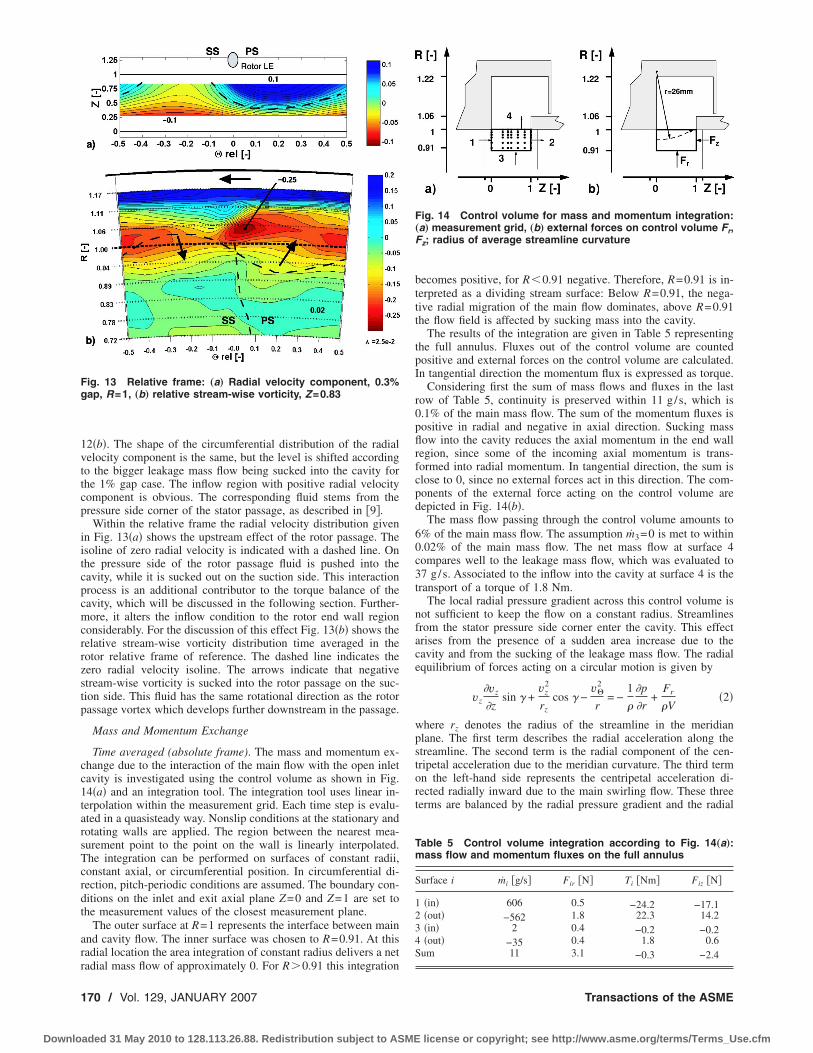
12�b�. The shape of the circumferential distribution of the radialvelocity component is the same, but the level is shifted accordingto the bigger leakage mass flow being sucked into the cavity forthe 1% gap case. The inflow region with positive radial velocitycomponent is obvious. The corresponding fluid stems from thepressure side corner of the stator passage, as described in �9�.

Within the relative frame the radial velocity distribution givenin Fig. 13�a� shows the upstream effect of the rotor passage. Theisoline of zero radial velocity is indicated with a dashed line. Onthe pressure side of the rotor passage fluid is pushed into thecavity, while it is sucked out on the suction side. This interactionprocess is an additional contributor to the torque balance of thecavity, which will be discussed in the following section. Further-more, it alters the inflow condition to the rotor end wall regionconsiderably. For the discussion of this effect Fig. 13�b� shows therelative stream-wise vorticity distribution time averaged in therotor relative frame of reference. The dashed line indicates thezero radial velocity isoline. The arrows indicate that negativestream-wise vorticity is sucked into the rotor passage on the suc-tion side. This fluid has the same rotational direction as the rotorpassage vortex which develops further downstream in the passage.

Mass and Momentum Exchange

Time averaged (absolute frame). The mass and momentum ex-change due to the interaction of the main flow with the open inletcavity is investigated using the control volume as shown in Fig.14�a� and an integration tool. The integration tool uses linear in-terpolation within the measurement grid. Each time step is evalu-ated in a quasisteady way. Nonslip conditions at the stationary androtating walls are applied. The region between the nearest mea-surement point to the point on the wall is linearly interpolated.The integration can be performed on surfaces of constant radii,constant axial, or circumferential position. In circumferential di-rection, pitch-periodic conditions are assumed. The boundary con-ditions on the inlet and exit axial plane Z=0 and Z=1 are set tothe measurement values of the closest measurement plane.

The outer surface at R=1 represents the interface between mainand cavity flow. The inner surface was chosen to R=0.91. At thisradial location the area integration of constant radius delivers a netradial mass flow of approximately 0. For R�0.91 this integration

becomes positive, for R�0.91 negative. Therefore, R=0.91 is in-terpreted as a dividing stream surface: Below R=0.91, the nega-tive radial migration of the main flow dominates, above R=0.91the flow field is affected by sucking mass into the cavity.

The results of the integration are given in Table 5 representingthe full annulus. Fluxes out of the control volume are countedpositive and external forces on the control volume are calculated.In tangential direction the momentum flux is expressed as torque.

Considering first the sum of mass flows and fluxes in the lastrow of Table 5, continuity is preserved within 11 g/s, which is0.1% of the main mass flow. The sum of the momentum fluxes ispositive in radial and negative in axial direction. Sucking massflow into the cavity reduces the axial momentum in the end wallregion, since some of the incoming axial momentum is trans-formed into radial momentum. In tangential direction, the sum isclose to 0, since no external forces act in this direction. The com-ponents of the external force acting on the control volume aredepicted in Fig. 14�b�.

The mass flow passing through the control volume amounts to6% of the main mass flow. The assumption m3=0 is met to within0.02% of the main mass flow. The net mass flow at surface 4compares well to the leakage mass flow, which was evaluated to37 g/s. Associated to the inflow into the cavity at surface 4 is thetransport of a torque of 1.8 Nm.

The local radial pressure gradient across this control volume isnot sufficient to keep the flow on a constant radius. Streamlinesfrom the stator pressure side corner enter the cavity. This effectarises from the presence of a sudden area increase due to thecavity and from the sucking of the leakage mass flow. The radialequilibrium of forces acting on a circular motion is given by

vz�vz

�zsin � +

vz2

rzcos � −

v�2

r= −

1

�

�p

�r+

Fr

�V�2�

where rz denotes the radius of the streamline in the meridianplane. The first term describes the radial acceleration along thestreamline. The second term is the radial component of the cen-tripetal acceleration due to the meridian curvature. The third termon the left-hand side represents the centripetal acceleration di-rected radially inward due to the main swirling flow. These threeterms are balanced by the radial pressure gradient and the radial

Fig. 13 Relative frame: „a… Radial velocity component, 0.3%gap, R=1, „b… relative stream-wise vorticity, Z=0.83

Fig. 14 Control volume for mass and momentum integration:„a… measurement grid, „b… external forces on control volume Fr,Fz; radius of average streamline curvature

Table 5 Control volume integration according to Fig. 14„a…:mass flow and momentum fluxes on the full annulus

Surface i mi �g/s� Fir �N� Ti �Nm� Fiz �N�

1 �in� 606 0.5 −24.2 −17.12 �out� −562 1.8 22.3 14.23 �in� 2 0.4 −0.2 −0.24 �out� −35 0.4 1.8 0.6Sum 11 3.1 −0.3 −2.4



external force. In this case, Eq. �2� can be simplified with the helpof the experimentally based assumption that the pitch angle of theinitial streamlines in surface 1 of Fig. 14�a� is approximately zerowhich leads to

vz2

rz

v�2

r= −

1

�

�p

�r+

Fr

�VCV�3�

The unknown in this equation is rz. All other terms can bederived out of the measurement volume. The second term on theleft-hand side is evaluated in taking the arithmetic average of allvalues within the control volume according to

v�2

r=

v�ijk2

rijk�4�

A representative radial pressure gradient is found in taking thepressure difference of each opposing pair of grid points, which layon surfaces 3 and 4. These local pressure differences are arith-metically averaged. The external radial force is taken from Table5. An average vz on surface 1 can be given to 19% of shroud rimspeed. From this approach a representative streamline with anaverage meridian radius of rz=26 mm is calculated. The stream-line is included in Fig. 14�b� as a dotted circular arc starting atmid-radial height of surface 1 with an assumed pitch angle �=0.The inflow of surface 1 connects well to the area around Z=0.8 ofsurface 4, where most of the inflow to the cavity happens �see alsoFig. 12�a��.

The axial component of the external force Fz �Table 5� is theresult of a static pressure increase across the cavity. To verify thisassumption a pressure force integration was performed taking themeasured static pressure at surfaces 1 and 2. The force calculatedwith the pressure difference becomes −2.6 N, which compareswell to the control volume integration. Across the cavity openinga positive axial pressure gradient is observed. The same procedureapplied to the main flow region �R�0.91� results in a negativeaxial pressure gradient as expected.

Additional insight could be gained by observing the quantitiesassociated to the in- and outflows across surface 4, which aresummarized in Table 6. As much as four times of the leakage massflow enters the cavity and convects up to 5 Nm of torque, 0.9 N ofradial momentum flux, and 1.5 N of axial momentum flux. Theoutflow of roughly three times the leakage mass flow conveys lessmomentum in all three components. However, the major contri-bution to the radial and axial momentum balance of the controlvolume are found in surfaces 1 and 2.

Time averaged (rotor relative frame). The associated fluxes tothe in- and outflow generated by the rotor pressure field are dis-cussed in this section. To do so, the surface integration of surface4 in Fig. 14 was performed in the relative frame of reference. Theradial velocity distribution of this surface is presented in Fig.13�a�. In comparison to Fig. 12�a�, the results are restricted to fiveaxial positions, which reduces the area covered by experimentalresults. The integration results are shown in Table 7. The massflow integration compares well to the results in Table 6 becausethe time averaged radial velocity components were adjusted to thefive-hole probe results. The radial component of momentumfluxes is larger than in the stator relative flow field. The axialcomponent of the momentum fluxes compares well to the results

in the absolute frame of reference. The important result here isthat the rotor in time average extracts torque from the cavity, sincethe sum of in- and outflows is negative.

Systematic Classification of Open Cavities

Characteristics of Open Cavities. There are three characteris-tics in which the open cavities differ �see also Table 8�:

(I) The strength of the radial pressure gradient at the interfacesurface due to the swirling main flow: Downstream of the statorthe swirl angle is constantly high inducing a much stronger radialpressure gradient �dCps /dR=0.02� than downstream of the rotor�dCps /dR=0.004�. The exit flow of the rotor depends on thepower extraction in which the stage is working. In the case ofmedium loaded stages the exit swirl of the rotor is small.

(II) The location at hub or tip: Radial pressure gradients arepointing either out of the cavity as is the case at the tip or pointinginto the cavity as at the hub. Low kinetic energy fluid migrates onlower radii according to the pressure gradient than fluid of higherkinetic energy. Therefore, the leakage fluid in cavity 3 under theinfluence of the radial pressure gradient set up in the main flowregion moves closer to the hub with negative radial velocity, thusforming the toroidal vortex there. The center of the vortex isfound at R=−0.12. At the tip, the low kinetic energy fluid withinthe cavity is sucked out of the cavity, such that the center of thetoroidal vortex in cavity 4 moves toward lower radii �R=1.06� andthe vortical flow is observed at the interface surface �R=1�.

(III) The leakage jet: The leakage jet in the exit cavities addsfluxes of axial and tangential momentum to the cavity flow. Inaddition, the mixing of the jet is a loss production mechanism.The leakage mass flow does no work to the rotor. This causes ahigher total temperature of the leakage flow than the main flowdownstream of the rotor. Downstream of the stator the total tem-perature of both fluxes is the same. Within the inlet cavities no jetis present, but end wall fluid is sucked into the labyrinth seal.Thus, the inlet cavity acts as a sink of axial and tangential mo-mentum.

Table 6 Mass and momentum fluxes across surface 4, abso-lute frame


4 �in, vr�0� 127 0.9 5.1 1.54 �out, vr�0� −92 −0.5 −3.3 −0.9Sum 35 0.4 1.8 0.6

Table 7 Mass and momentum fluxes across surface 4, rotorrelative


4 �in, vr�0� 148 1.6 1.1 1.44 �out, vr�0� −110 −0.6 −1.3 −0.9Sum 38 1.0 −0.2 0.5

Table 8 Characteristics of open cavities in turbines

No.SwirlI

PositionII

JetIII

Incidencea�

Loss productionb�

1 Hub �=0 degsucking

Sucking of BL at hub,smaller hub loss core andsecondary flows in rotorpassage

2 Tip Tjo�Tm

o �=−30 deg Mixing of the jet withcavity and main flowJet increases. BL-thickness

3 �� Hub Tjo=Tm

o ��=−70 deg Mixing of the jet withcavity and main flowSecondary flowdevelopment in rotorpassage

4 �� Tip ��=−7 degsucking

Vortex stretching, wallfriction in cavitySecondary flowdevelopment in rotor



Influence on Main Flow and Performance. Each of the opencavities differs in their influence on the main flow and the perfor-mance of the machine. The effects discussed here are the changeof incidence and the loss production mechanisms induced by thecorresponding cavity �Table 8�.

(a) Incidence angle to the end wall regions of downstreamblade rows: The leakage jet in cavities 2 and 3 causes a negativeincidence due to the mismatch of the velocity triangles. At theinlet to the downstream blade row the incidence angles at the endwall regions are of the order of −30 deg and −70 deg. Cavity 4induces negative incidence via sucking of circumferential momen-tum. Evaluating the flow with the help of a control volume analy-sis and further modeling the flow predicts an incidence angle of−7 deg for the 1% gap case. Cavity 1 is estimated to induce noincidence since the exit flow of the rotor, which is sucked into thehub labyrinth, has no circumferential momentum.

(b) Loss production mechanisms: Sucking of boundary layerfluid at cavity 1 can be beneficial, since a thinner boundary layerenters the stator hub and thus less secondary flow is generated. Incavity 4 the effect of sucking may be less beneficial since thecavity is pressure loaded and interaction mass flows of up to fourtimes the leakage mass flow do leave the cavity again. Theseinteraction outflows then enter into the rotor tip region enhancingthe secondary flow development with a sheet of positive stream-wise vorticity at the suction side of the rotor passage �see Fig.13�b��. In addition cavity 4 contributes to the loss production viavortex stretching and enhanced wall friction due to the toroidalvortex system. In cavities 2 and 3 the leakage jet mixes with thecavity and main flow in addition to generating strong negativeincidences to the downstream blade rows.

Design ProposalsIn this section the gained flow understanding is used to propose

design changes and to quantify a beneficial effect if possible.

Cavity 2. The approach for cavity 2 is to optimize the leakagemixing process. As reported in the previous section, 6.7% of thestage losses are attributable to the mixing. In a further step ofinvestigation the mixing calculation model was used to investigatethree cases of leakage mass distribution. The cases are visualizedin Fig. 15. The upper distribution of velocity vectors belongs tothe experimentally found situation.

Case 1: Homogeneous distribution of velocity vectors.Case 2: Mirrored at �rel=0.Case 3: Most of the leakage mass flow into the rotor wake.By varying the leakage vector distribution the leakage mass

flow as well as the momentum fluxes were kept constant. Fromthis approach, an improvement of 0.1% in efficiency is predicted

for cases 1 and 3 in comparison to the experiment. Case 2 doesnot show improvements. In case 1, downstream blade rows re-ceive a more homogeneous inflow, which is in accordance toDawes’ comment about design goals in end wall regions �13�.Case 3 seems to be beneficial, since feeding the leakage flow intothe wake reduces nonuniformity in the main flow and thereforereduces the mixing contribution in step 2 of the mixing model.Despite the rough assumptions applied to the mixing model, theresults do indicate possible improvements.

In order to achieve a leakage jet distribution similar to case 3, adesign modification for a nonaxisymmetric shroud contour is pro-posed, as shown in Fig. 16. The gap variation around the circum-ference varies between completely closed at mid-pitch and open atthe rotor trailing edge position. The gap area is kept the same as inthe 1% gap case. The leakage mass flow passing through the sealgap below the trailing edge will end up mixing with the rotorwake, when the leakage fluid leaves the cavity. Thus the leakageflow is used to reduce nonuniformities in the end wall region ofthe turbine.

The design of the nonaxisymmetric gap depends on the re-entrybehavior of the leakage flow. A simple model is proposed to de-scribe the circumferential position of the maximum gap relative tothe rotor trailing edge ��relG� as depicted in Fig. 17. The modeluses three parameters:

�1� The characteristic length scale of the problem is the axialgap width of the exit cavity zcav.

�2� The average relative flow angle of the leakage flow fromlast seal gap to the re-entry into main flow �L.

�3� The relative flow angle of the main flow at the rotor tip �T.

In addition, the designer has to define the location along theconvective path of the wake, where it is desirable to let the leak-age flow interact with the wake �wake window�. These parameterscombine to the nondimensional circumferential position of themaximum gap of

�relG =zcav

p�tan �T − 1.3 tan �L� �5�

Fig. 15 Rotor relative descriptive flow model and two-stepmixing calculation of leakage and main flow

Fig. 16 Nonaxisymmetric shroud design in cavity 2: „a… up-stream view of the last sealing gap, „b… side view

Fig. 17 Simple model for shroud design



The local blade pitch is denoted with p. The factor 1.3 describesthe geometric fact of this configuration, that the leakage jet startsat a more upstream axial position than the wake �seal gap positionversus trailing edge position�. For this test case and cavity theposition for the maximum gap results in �relG=0.05, which isvery close to the trailing edge position.

Cavity 3. In cavity 3, the same principal as described above forcavity 2 can be applied. Thus a more uniform flow distributionwould be generated at the inlet to the rotor hub and the leakagemixing losses would be reduced. As reported in �7�, inserts intothe exit cavities were investigated preventing the toroidal vortexto develop and guiding the leakage flow back into the main flow.The upstream effect of the rotor passage onto the leakage flow anddistribution on the incoming vorticity field has been shown in theexperimental results for cavity 4. In order to control the mixingand the re-entry of the leakage flow at the hub the authors proposeto extend the idea of nonaxisymmetric end wall contouring asdescribed, e.g., in �14� or in �15� into the exit cavity and combineit with the nonaxisymmetric design of the shroud trailing edge andlast seal gap. The resulting design is depicted in Fig. 18. The gapshape is highlighted in green. The maximum gap is shifted to thesuction side of the stator passage. Thus the leakage flow can beexpected to reenter into the main duct at the circumferential posi-tion of the stator wake.

Using the approach presented for cavity 2, an equation for thehub exit cavity can be given

�G =zcav

p�1.3 tan L − tan H� �6�

Taking an average flow angle of the leakage fluid of L=75 deg and the swirl angle at the hub H=67.5 deg, this resultsin a circumferential position of the maximum gap of �G=0.8,relative to the stator trailing edge position. The underlying as-sumption is that the average flow angle of the leakage L remainsthe same with the inserts. The beneficial effect will be of the sameorder as in cavity 2, i.e., around 0.1% absolute turbine efficiency.

The nonaxisymmetric insert is designed such that the leakageflow is guided into the rotor passage in a favorable way. Thedesign shifts the incoming leakage fluid onto the suction side ofthe rotor passage. This aims at two effects:

�1� The leakage fluid is found on the suction side, thus thesecondary flow development in the passage due to themovement of the low kinetic energy fluid in the cross pas-sage pressure gradient is reduced. Wall shear stresses at theend wall due to the development of a new boundary layercould be reduced.

�2� The distribution of the leakage fluid to the suction sidereduces the likelihood of a separation bubble at the pressure

side of the rotor leading edge due to the strong negativeincidence of the leakage flow. Instead of leakage fluid, athin boundary layer of main flow fluid is hitting the rotorleading edge at the correct angle of attack.

Cavity 4. The inlet cavity to the rotor tip labyrinth seal issubject to large in- and outflows as described in detail in �9�.Three approaches will be discussed, which are considered to befavorable in terms of loss production and reduction of unsteadyinteraction and secondary flows.

�1� Nonaxisymmetric end wall contouring in the stator passageis a promising tool to reduce secondary losses as reported in �16�.This approach has the potential to reduce the inflow and outflowdue to the end wall curvature. Applied to the inlet cavity thiswould mean that the end wall on the pressure side would have tobe convex. The induced static pressure drop would provide thefluid in the pressure side corner with additional kinetic energy.Thus the fluid particles tend to penetrate less into the cavity. Thesame target can be followed by introducing a local lean to thestator trailing edge, which would cause a local load increase. Thepressure side corner fluid then would experience an additionalradial force due to the imposed local static pressure gradient. Alarger radius of streamline curvature is resulting from this and lessamount of fluid is penetrating into the cavity.

�2� The lip on the stator side of the cavity, as depicted in Fig.19, is designed to reduce the circumferential wake as found in �9�and to turn the fluid at the edge of the toroidal vortex into axialdirection. The static pressure gradients originating from the statortrailing edge and acting on the interaction zone are reduced due tothe potential field decay.

�3� The shroud leading edge depicted in Fig. 19 is designed toreduce the interaction flow across the cavity-to-main flow inter-face. One expected effect would be that the radial velocity distri-bution as presented in Fig. 13�a� is more homogeneous and thepeak radial velocities are reduced. On the pressure side of therotor passage the shroud leading edge is positioned at a higherradius than on the suction side. The effect of this is that stream-lines of a lower curvature are entering on the pressure side. Lessfluid is pushed into the cavity at this point. On the suction side,the cavity fluid has to reach lower radii in order to be sucked intothe rotor passage. In terms of streamline curvature, more fluid ispushed into the cavity at the suction side than on the pressure side.

The design modification described above with the help of Fig.19 can be inverted, i.e., it is the goal to enhance the interactionflow such that the inlet stream-wise vorticity distribution as found

Fig. 18 Nonaxisymmetric shroud and cavity design, cavity 3:„a… upstream view, Z=0.5, „b… side view with nonaxisymmetricinsert

Fig. 19 Shroud leading edge design for reduced rotor passageto cavity flow interaction



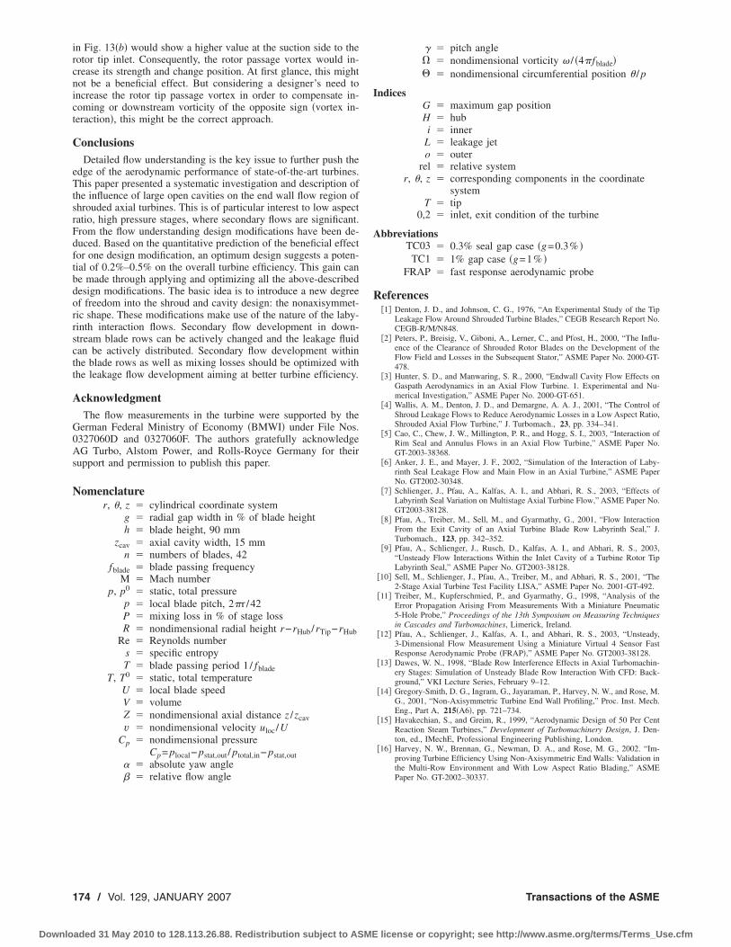
in Fig. 13�b� would show a higher value at the suction side to therotor tip inlet. Consequently, the rotor passage vortex would in-crease its strength and change position. At first glance, this mightnot be a beneficial effect. But considering a designer’s need toincrease the rotor tip passage vortex in order to compensate in-coming or downstream vorticity of the opposite sign �vortex in-teraction�, this might be the correct approach.

ConclusionsDetailed flow understanding is the key issue to further push the

edge of the aerodynamic performance of state-of-the-art turbines.This paper presented a systematic investigation and description ofthe influence of large open cavities on the end wall flow region ofshrouded axial turbines. This is of particular interest to low aspectratio, high pressure stages, where secondary flows are significant.From the flow understanding design modifications have been de-duced. Based on the quantitative prediction of the beneficial effectfor one design modification, an optimum design suggests a poten-tial of 0.2%–0.5% on the overall turbine efficiency. This gain canbe made through applying and optimizing all the above-describeddesign modifications. The basic idea is to introduce a new degreeof freedom into the shroud and cavity design: the nonaxisymmet-ric shape. These modifications make use of the nature of the laby-rinth interaction flows. Secondary flow development in down-stream blade rows can be actively changed and the leakage fluidcan be actively distributed. Secondary flow development withinthe blade rows as well as mixing losses should be optimized withthe leakage flow development aiming at better turbine efficiency.

AcknowledgmentThe flow measurements in the turbine were supported by the

German Federal Ministry of Economy �BMWI� under File Nos.0327060D and 0327060F. The authors gratefully acknowledgeAG Turbo, Alstom Power, and Rolls-Royce Germany for theirsupport and permission to publish this paper.

Nomenclaturer, �, z cylindrical coordinate system

g radial gap width in % of blade heighth blade height, 90 mm

zcav axial cavity width, 15 mmn numbers of blades, 42

fblade blade passing frequencyM Mach number

p, p0 static, total pressurep local blade pitch, 2�r /42P mixing loss in % of stage lossR nondimensional radial height r−rHub/rTip−rHub

Re Reynolds numbers specific entropyT blade passing period 1/ fblade

T, T0 static, total temperatureU local blade speedV volumeZ nondimensional axial distance z /zcavv nondimensional velocity uloc /U

Cp nondimensional pressureCp= plocal− pstat,out / ptotal,in− pstat,out

absolute yaw angle� relative flow angle

� pitch angle� nondimensional vorticity � / �4�fblade�� nondimensional circumferential position � / p

IndicesG maximum gap positionH hubi inner

L leakage jeto outer

rel relative systemr, �, z corresponding components in the coordinate

systemT tip

0,2 inlet, exit condition of the turbine

AbbreviationsTC03 0.3% seal gap case �g=0.3% �

TC1 1% gap case �g=1% �FRAP fast response aerodynamic probe

References�1� Denton, J. D., and Johnson, C. G., 1976, “An Experimental Study of the Tip

Leakage Flow Around Shrouded Turbine Blades,” CEGB Research Report No.CEGB-R/M/N848.

�2� Peters, P., Breisig, V., Giboni, A., Lerner, C., and Pfost, H., 2000, “The Influ-ence of the Clearance of Shrouded Rotor Blades on the Development of theFlow Field and Losses in the Subsequent Stator,” ASME Paper No. 2000-GT-478.

�3� Hunter, S. D., and Manwaring, S. R., 2000, “Endwall Cavity Flow Effects onGaspath Aerodynamics in an Axial Flow Turbine. 1. Experimental and Nu-merical Investigation,” ASME Paper No. 2000-GT-651.

�4� Wallis, A. M., Denton, J. D., and Demargne, A. A. J., 2001, “The Control ofShroud Leakage Flows to Reduce Aerodynamic Losses in a Low Aspect Ratio,Shrouded Axial Flow Turbine,” J. Turbomach., 23, pp. 334–341.

�5� Cao, C., Chew, J. W., Millington, P. R., and Hogg, S. I., 2003, “Interaction ofRim Seal and Annulus Flows in an Axial Flow Turbine,” ASME Paper No.GT-2003-38368.

�6� Anker, J. E., and Mayer, J. F., 2002, “Simulation of the Interaction of Laby-rinth Seal Leakage Flow and Main Flow in an Axial Turbine,” ASME PaperNo. GT2002-30348.

�7� Schlienger, J., Pfau, A., Kalfas, A. I., and Abhari, R. S., 2003, “Effects ofLabyrinth Seal Variation on Multistage Axial Turbine Flow,” ASME Paper No.GT2003-38128.

�8� Pfau, A., Treiber, M., Sell, M., and Gyarmathy, G., 2001, “Flow InteractionFrom the Exit Cavity of an Axial Turbine Blade Row Labyrinth Seal,” J.Turbomach., 123, pp. 342–352.

�9� Pfau, A., Schlienger, J., Rusch, D., Kalfas, A. I., and Abhari, R. S., 2003,“Unsteady Flow Interactions Within the Inlet Cavity of a Turbine Rotor TipLabyrinth Seal,” ASME Paper No. GT2003-38128.

�10� Sell, M., Schlienger, J., Pfau, A., Treiber, M., and Abhari, R. S., 2001, “The2-Stage Axial Turbine Test Facility LISA,” ASME Paper No. 2001-GT-492.

�11� Treiber, M., Kupferschmied, P., and Gyarmathy, G., 1998, “Analysis of theError Propagation Arising From Measurements With a Miniature Pneumatic5-Hole Probe,” Proceedings of the 13th Symposium on Measuring Techniquesin Cascades and Turbomachines, Limerick, Ireland.

�12� Pfau, A., Schlienger, J., Kalfas, A. I., and Abhari, R. S., 2003, “Unsteady,3-Dimensional Flow Measurement Using a Miniature Virtual 4 Sensor FastResponse Aerodynamic Probe �FRAP�,” ASME Paper No. GT2003-38128.

�13� Dawes, W. N., 1998, “Blade Row Interference Effects in Axial Turbomachin-ery Stages: Simulation of Unsteady Blade Row Interaction With CFD: Back-ground,” VKI Lecture Series, February 9–12.

�14� Gregory-Smith, D. G., Ingram, G., Jayaraman, P., Harvey, N. W., and Rose, M.G., 2001, “Non-Axisymmetric Turbine End Wall Profiling,” Proc. Inst. Mech.Eng., Part A, 215�A6�, pp. 721–734.

�15� Havakechian, S., and Greim, R., 1999, “Aerodynamic Design of 50 Per CentReaction Steam Turbines,” Development of Turbomachinery Design, J. Den-ton, ed., IMechE, Professional Engineering Publishing, London.

�16� Harvey, N. W., Brennan, G., Newman, D. A., and Rose, M. G., 2002. “Im-proving Turbine Efficiency Using Non-Axisymmetric End Walls: Validation inthe Multi-Row Environment and With Low Aspect Ratio Blading,” ASMEPaper No. GT-2002–30337.



T. Povey

T. V. Jones

M. L. G. Oldfield

Department of Engineering Science,University of Oxford,

Parks Road,Oxford OX1 3PJ, UK

On a Novel Annular SectorCascade TechniqueAn advanced technique for establishing pressure boundary conditions in annular sectorcascade experiments has been developed. This novel technique represents an improve-ment over previous methods and provides the first means by which annular sector bound-ary conditions that are representative of those which develop in an annular cascade canbe established with a high degree of satisfaction. The technique will enable cascadedesigners to exploit the obvious advantages of annular sector cascade testing: the re-duced cost of both facility manufacture and facility operation and the use of engine partsin place of two-dimensional counterparts. By employing an annular sector of deswirlvanes downstream of the annular sector of test vanes, the radial pressure gradient estab-lished in the swirling flow downstream of the test vanes is not disturbed. The deswirl vaneexit flow—which has zero swirl velocity—can be exhausted without unsteadiness, andwithout the risk of separation, into a plenum at constant pressure. The pressure ratioacross the annular sector of test vanes can be tuned by adjusting the throat area at thedeswirl vane exit plane. Flow conditioning systems which utilize the Oxford deswirl vanetechnology have previously been used to set pressure boundary conditions downstream offully annular cascades in both model and engine scale (the Isentropic Light Piston Fa-cility at Farnborough) experimental research facilities (Povey, T., Chana, K. S., Oldfield,M. L. G., Jones, T. V., and Owen, A. K., 2001, Proceedings of the ImechE Advances inFluid Machinery Design Seminar, London, June 13; Povey, T., Chana, K. S., Jones, T. V.,and Oldfield, M. L. G., 2003, Advances of CFD in Fluid Machinery Design, ImechEProfessional Engineering, London, pp. 65–94). The deswirl vane is particularly suited tothe control of highly whirling transonic flows. It has been demonstrated by direct com-parison of aerodynamic measurements from fully annular and annular sector experimentsthat the use of a deswirl vane sector for flow conditioning at the exit of an annular sectorcascade represents an attractive novel solution to the boundary condition problem. Theannular sector technique is now described. �DOI: 10.1115/1.2372766�

IntroductionIn the annular cascade experiment, the nature of secondary flow

development depends upon both inlet and exit-flow conditions.Where a nozzle guide vane row is tested in isolation—in a sta-tionary cascade—engine-representative pressure boundary condi-tions are often difficult to achieve. Radial pressure gradients, es-tablished in regions of swirling flow, affect the growth ofsecondary flows and, indeed, the spanwise velocity distribution atthe vane exit plane. Several methods have been developed to es-tablish the correct radial pressure gradient at the exit of annularcascade facilities, although many of these are somewhatunsatisfactory—a common problem is that of unsteady flow sepa-ration downstream of the test vane.

An alternative to annular cascade testing is the use of a fixedlinear cascade of vanes, a technique that is attractive because test-ing is possible at lower mass flow rates—a smaller number of testvanes can be used at the same chord size. In the linear cascade,radial pressure gradients are not established, and secondary flowsdo not develop as they would in a working engine. This meansthat radial distributions of total pressure loss and whirl angle areunrepresentative of engine conditions. In addition, surface heat-transfer rate distributions, which are strongly influenced by thesecondary flow structure, are nonrepresentative of engine condi-tions. An additional shortcoming is that only geometrically sim-plified �usually two dimensional� designs can be tested, whereasin annular cascade experiments the exact three-dimensional vane

profiles, even engine parts, can be used. Another difficulty is thatof establishing truly periodic inlet and exit-flow conditions,which, being established automatically in the annular facility, canbe achieved in a linear cascade only when a very large number ofvanes is used.

The sidewalls of the inflow and exit ducts of a linear cascadeexert a strong influence on the streamline pattern within the cas-cade, and techniques such as variable wall suction and flexiblesidewalls have been employed to tune the inlet and exit-flow con-ditions. Achieving even approximately periodic conditions is gen-erally problematic, however. A very comprehensive review of ad-vanced techniques applicable to both linear and annular cascadetesting has been published by AGARD �1�.

Annular sector cascade testing is a technique that combines theadvantages of both the annular and linear cascade testing methods.Actual engine components can be tested, and the radial pressuregradients established in regions of swirling flow ensure secondaryflows develop as they would in an operating engine. Model andtesting costs for annular sector cascades are considerably lowerthan for their fully annular equivalents. Annular sector cascadetesting is, however, relatively uncommon, as the designer is facedwith the dual challenges of establishing vane-to-vane periodicity,and of maintaining the radial pressure gradient in the sector cas-cade exit flow. To date, these problems have not been satisfacto-rily resolved, and, consequently, the potential advantages of annu-lar sector testing have so far not been fully enjoyed.

Annular Sector FacilitiesBecause the annular sector technique is little used, there is very

little literature concerning the methods of designing and operatingsuch facilities. Over the years, however, a few annular sector fa-cilities have been developed, primarily for studies of cooling flow




effectiveness and for measurements of vane surface heat transfercoefficient. An early example is the NASA Lewis Research CentreHot Section Facility �2�, a 23 deg annular sector cascade in whichengine components were used.

More recently, a high-pressure high-temperature annular sectorfacility was commissioned at ABB STAL—Sweden �3�. The ini-tial configuration was a four-passage, 40 deg, annular sector ofhigh-pressure nozzle guide vanes operated without film cooling. Alarge compressor unit was used, capable of delivering 10 kg s−1 ata pressure of 20 bar and a temperature of 200°C. The mainstreamflow was heated in a combustion chamber—oil-fired burner—totemperatures of up to 800°C. The designers took considerablecare in establishing engine-representative inlet boundary condi-tions, and, by introducing cooler air though the hub and the caseplatforms upstream of the test vanes, the radial temperature gra-dients that are present at the exit of a combustor were modeled.By using the technique of hot-wire anemometry, the freestreamturbulence intensity was characterized—4–5%. The test vaneswere instrumented with thermocouples. An infrared camera wasalso used to conduct temperature measurements. By operating theexperiment in several different modes, it was possible to calculatethe cooling effectiveness, and the internal and external heat trans-fer coefficients. A short exit duct with an abrupt expansion wasused downstream of the test vanes.

An interesting annular sector study was conducted by Wiersand Fransson �4�, who investigated the influence on cross-sectorperiodicity of various tailboard and diffuser geometries. The facil-ity that was used for the study was a five-passage annular sector,with two—smaller—bypass channels. The facility could operatecontinuously, with air supplied by 1 MW compressor at up to4.7 kg s−1 at a pressure of 4 bar. The inlet temperature could bevaried between 30 and 180°C. An adjustable valve was used toset the downstream pressure. Very detailed measurements wereconducted of the distributions of vane surface pressure, and endwall pressure. To quantify the degree to which periodicity hadbeen achieved across the sector, measurements of the circumfer-ential pressure distribution were conducted on the hub and casewalls at axial distances from the trailing edge equal to 35% and9% of the vane axial chord, respectively. Measurements were con-ducted only across the center two passages of the cascade. Testswere conducted with a diffuser with a 12 deg flare angle, with anabrupt expansion, and with various combinations of right-handand left-hand tailboards. The diffusers were in both cases situatedat axial distances equal to 190% of the axial chord downstream ofthe test vanes.

Interestingly, after extensive experimentation, the authors foundthat the best periodicity was obtained when the flow was allowedto exhaust as a free jet into the downstream plenum, with no flowconditioning whatsoever. For the two passages for which mea-surements were taken, the peak isentropic Mach numbers at hubwere 0.87 and 0.84. The corresponding Mach numbers at the casewere 0.81 and 0.80. The experiments demonstrate that reasonablyperiodic flow can be obtained across at least a limited part of anannular sector, by using the free-jet approach. The Wiers andFransson �4� investigation is probably the most comprehensiveaerodynamic survey in an annular sector to date.

At the Royal Institute of Technology in Sweden, an annularsector facility has been developed for studies of the aeroelasticbehaviour of low-pressure rotor blades when subject to forcing�5�. To allow some control over the periodicity of the flow-fielddownstream of the �nine passage� annular sector of rotor blades,semi-flexible—polyurethane—sidewalls were employed. To miti-gate the problems associated with exhausting swirling flow into aconstant pressure plenum, a long exit duct was used.

A new technique of using an annular sector of half-impulse �seebelow� type deswirl vanes to condition the exit flow of an annularsector cascade has been developed. This has been shown toachieve excellent vane-to-vane periodicity for even a small num-ber of test vane passages—five—while maintaining the radial

pressure field established in the swirling flow downstream of thetest vanes. In addition, the technique eliminates the need for anextended exit duct downstream of the test vanes: the flow can beexhausted without unsteadiness to a plenum at constant pressure.

Pressure Gradients and Secondary Flow DevelopmentThe radial pressure gradient established in regions of swirling

flow contributes to the overall inviscid pressure field in such away as to promote growth of the case secondary flow but to in-hibit growth of the hub secondary flow. This is shown diagram-matically in Fig. 1—arrows point from higher to lower pressure.Although radial pressure gradients arise naturally in swirling flow,annular cascade experiments normally include only isolated tur-bine stages—or part stages—and the designer is therefore facedwith the challenge of establishing representative conditions at in-let and exit of the cascade—the conditions that would exist in aworking engine—which, in general, will be different from thoseconditions that would be achieved in the experiment in the ab-sence of additional flow conditioning.

Cascade Inlet Conditions. In the working engine environment,there are radial and circumferential gradients in the combustorexit flow of total temperature, total pressure and free stream tur-bulence. In general, however, there is little swirl at combustorexit, and high-pressure nozzle guide vanes are usually designedfor axial inlet flow. There have been very few experiments to datein which spatial variations in inlet flow properties have been simu-lated. In principle, it would be possible to establish a radial totalpressure gradient upstream of a turbine stage by using gauzes withvarying porosity, a technique that has been applied in studies ofcompressors but so far not of turbines. Similarly, if required, aninlet swirl angle distribution could be generated using inlet guidevanes, although wakes and secondary flows would present prob-lems for the designer of such a system. In experiments in whichheat transfer rates are to be measured, the importance is recog-nized of establishing the correct free stream turbulence intensity,and it is relatively common to include a turbulence grid upstream

Fig. 1 Development of secondary flows in an annular cascade



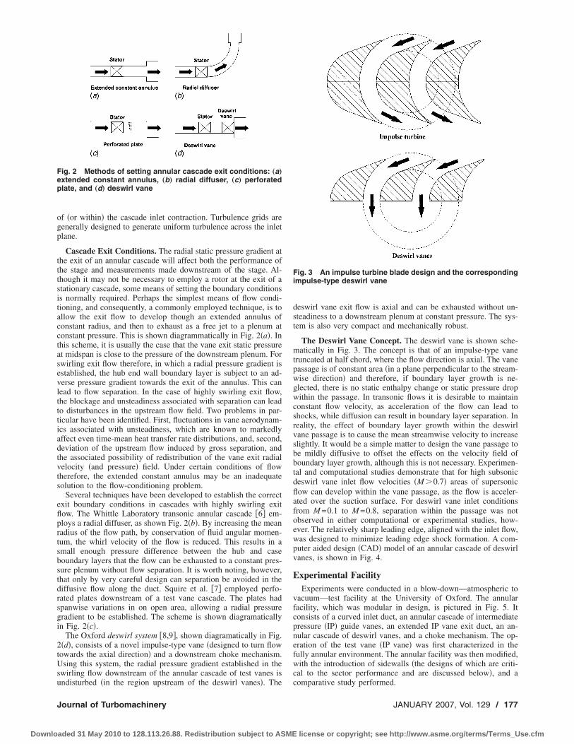
of �or within� the cascade inlet contraction. Turbulence grids aregenerally designed to generate uniform turbulence across the inletplane.

Cascade Exit Conditions. The radial static pressure gradient atthe exit of an annular cascade will affect both the performance ofthe stage and measurements made downstream of the stage. Al-though it may not be necessary to employ a rotor at the exit of astationary cascade, some means of setting the boundary conditionsis normally required. Perhaps the simplest means of flow condi-tioning, and consequently, a commonly employed technique, is toallow the exit flow to develop though an extended annulus ofconstant radius, and then to exhaust as a free jet to a plenum atconstant pressure. This is shown diagrammatically in Fig. 2�a�. Inthis scheme, it is usually the case that the vane exit static pressureat midspan is close to the pressure of the downstream plenum. Forswirling exit flow therefore, in which a radial pressure gradient isestablished, the hub end wall boundary layer is subject to an ad-verse pressure gradient towards the exit of the annulus. This canlead to flow separation. In the case of highly swirling exit flow,the blockage and unsteadiness associated with separation can leadto disturbances in the upstream flow field. Two problems in par-ticular have been identified. First, fluctuations in vane aerodynam-ics associated with unsteadiness, which are known to markedlyaffect even time-mean heat transfer rate distributions, and, second,deviation of the upstream flow induced by gross separation, andthe associated possibility of redistribution of the vane exit radialvelocity �and pressure� field. Under certain conditions of flowtherefore, the extended constant annulus may be an inadequatesolution to the flow-conditioning problem.

Several techniques have been developed to establish the correctexit boundary conditions in cascades with highly swirling exitflow. The Whittle Laboratory transonic annular cascade �6� em-ploys a radial diffuser, as shown Fig. 2�b�. By increasing the meanradius of the flow path, by conservation of fluid angular momen-tum, the whirl velocity of the flow is reduced. This results in asmall enough pressure difference between the hub and caseboundary layers that the flow can be exhausted to a constant pres-sure plenum without flow separation. It is worth noting, however,that only by very careful design can separation be avoided in thediffusive flow along the duct. Squire et al. �7� employed perfo-rated plates downstream of a test vane cascade. The plates hadspanwise variations in on open area, allowing a radial pressuregradient to be established. The scheme is shown diagramaticallyin Fig. 2�c�.

The Oxford deswirl system �8,9�, shown diagramatically in Fig.2�d�, consists of a novel impulse-type vane �designed to turn flowtowards the axial direction� and a downstream choke mechanism.Using this system, the radial pressure gradient established in theswirling flow downstream of the annular cascade of test vanes isundisturbed �in the region upstream of the deswirl vanes�. The

deswirl vane exit flow is axial and can be exhausted without un-steadiness to a downstream plenum at constant pressure. The sys-tem is also very compact and mechanically robust.

The Deswirl Vane Concept. The deswirl vane is shown sche-matically in Fig. 3. The concept is that of an impulse-type vanetruncated at half chord, where the flow direction is axial. The vanepassage is of constant area �in a plane perpendicular to the stream-wise direction� and therefore, if boundary layer growth is ne-glected, there is no static enthalpy change or static pressure dropwithin the passage. In transonic flows it is desirable to maintainconstant flow velocity, as acceleration of the flow can lead toshocks, while diffusion can result in boundary layer separation. Inreality, the effect of boundary layer growth within the deswirlvane passage is to cause the mean streamwise velocity to increaseslightly. It would be a simple matter to design the vane passage tobe mildly diffusive to offset the effects on the velocity field ofboundary layer growth, although this is not necessary. Experimen-tal and computational studies demonstrate that for high subsonicdeswirl vane inlet flow velocities �M �0.7� areas of supersonicflow can develop within the vane passage, as the flow is acceler-ated over the suction surface. For deswirl vane inlet conditionsfrom M =0.1 to M =0.8, separation within the passage was notobserved in either computational or experimental studies, how-ever. The relatively sharp leading edge, aligned with the inlet flow,was designed to minimize leading edge shock formation. A com-puter aided design �CAD� model of an annular cascade of deswirlvanes, is shown in Fig. 4.

Experimental FacilityExperiments were conducted in a blow-down—atmospheric to

vacuum—test facility at the University of Oxford. The annularfacility, which was modular in design, is pictured in Fig. 5. Itconsists of a curved inlet duct, an annular cascade of intermediatepressure �IP� guide vanes, an extended IP vane exit duct, an an-nular cascade of deswirl vanes, and a choke mechanism. The op-eration of the test vane �IP vane� was first characterized in thefully annular environment. The annular facility was then modified,with the introduction of sidewalls �the designs of which are criti-cal to the sector performance and are discussed below�, and acomparative study performed.

Fig. 2 Methods of setting annular cascade exit conditions: „a…extended constant annulus, „b… radial diffuser, „c… perforatedplate, and „d… deswirl vane

Fig. 3 An impulse turbine blade design and the correspondingimpulse-type deswirl vane



The IP vane count was 26 �0.270 engine scale�, and 26 deswirlvanes were used for downstream flow conditioning. Both annuliof vanes were constructed from resin using the technique of ste-reolithography. The predicted area-mean IP vane exit-flow anglewas 71.9 deg, and the area-mean exit Mach number was 0.76.

The design details and operating conditions of the facility aresummarized in Table 1, below. The predicted deswirl vane inletflow conditions were based on the results of a computationalsimulation conducted using the Rolls-Royce code JA63. The IPvane, IP vane exit duct, and deswirl system, were all included inthe computational model.

The annular deswirl vane cascade and rotatable choke mecha-nism have been shown by experiment �8,9� to reproduce the radial

pressure gradients downstream of an annular cascade of test vanesthat exist in the working engine environment—in which the IPvane operates as part of an IP stage.

This paper presents experiments which demonstrate the useful-ness of the deswirl system, not only in the fully annular environ-ment, but also in the annular sector environment. The fully annu-lar model test facility was modified with the introduction ofshaped sidewalls so that the flow in a five-passage annular sectorcould be studied. If the deswirl system is used for flow condition-ing downstream of a test vane, the problem of achieving enginerepresentative flow conditions in the annular sector environmentreduces to the problem of establishing periodicity. The degree ofperiodicity that is achieved is highly dependent on the sidewalldesign.

The influence of sidewall profile on the sector flow field and onthe periodicity at the IP vane exit-plane within the sector wasassessed by comparing measurements conducted in sectors withdifferent sidewall designs to measurements conducted in the fullyannular facility. Two sector designs were investigated. Each in-cluded five passages �six IP vanes and six deswirl vanes� andsubtended an angle of 69.2 deg at the facility axis. Sector side-walls were designed and manufactured �stereolithography hard-ened resin� so that they could be attached within the annular exitduct of the test facility, thereby partitioning a sector of vanes.Thus, the same instrumentation could be used for both fully an-nular and annular sector tests. A CAD drawing of a four-passagesector �IP vanes removed� is presented in Fig. 6 �a five-passagesector was used for experiments reported in this paper�.

The angular displacement between the IP vane sector and thedeswirl vane sector was dependent on the angle of the sidewalls

Fig. 4 Annular cascade of deswirl vanes

Fig. 5 The working section of the test facility

Table 1 Facility design details and operating conditions

Parameter Target

IP vane inlet total pressure, bar 1.00IP vane inlet total temperature �K� 291Inlet Mach number 0.45Inlet whirl angle 0°IP vane axial chord �midspan� �mm� 23.0Linear scale factor 0.270IP vane throat area �m2� 3.565�10−3

Deswirl vane throat area �m2� 3.967�10−3

Re based on IP vane axial chord �at M =0.76� 2.88�105

Mass flow rate �at M =1.0� �kg s−1� 0.853Predicted deswirl vane inlet Mach number 0.76Predicted deswirl vane inlet whirl �deg� 71.9Deswirl vane LE metal angle �deg� 63.1Design incidence angle �deg� 8.8Deswirl vane hub/case chord, mm 15.48/15.48Deswirl vane hub/case pitch �mm� 18.34/23.49



relative to the axis. The annuli of vanes could be rotated relativeto each other to ensure exact periodicity with sector sidewall de-signs of different angles.

Sidewall Design Philosophy. The principal objective in thedesign of an annular sector cascade is to reproduce the flow of theequivalent fully annular facility. It is desirable therefore for thesidewalls to have the minimum influence on the natural develop-ment of the flow streamlines downstream of the test vane cascade;that is, the streamlines should be allowed to develop as theywould in the equivalent fully annular facility. The sidewall de-signs must necessarily be constrained, however, by the require-ments of starting at the trailing edge line of the test vane andterminating at the leading edge line of the deswirl vane. In gen-eral, the test vane might have both axial and tangential lean andmay also be swept. A swept vane, for example, would dictatesidewall designs that, at least on the upstream side of the sector,were convex on one side of the sector and concave on the other, soas to ensure smooth flow paths at the trailing edges of the left-hand and right-hand test vanes, at the vane-sidewall join. Thegeneral shape of the sector is determined by the sidewall angles,however, and the variation of these angles in both the radial andaxial directions.

Consider a vane cascade for which the downstream streamlinepattern is well characterized by either measurement or CFD mod-eling. In general, there will exist both radial and circumferentialvariations in velocity, whirl angle, and yaw angle, at the exit planeof the cascade, and in the downstream flow field. For this complexflow field, an obvious starting point in the sidewall design processmight be to match the angle of both sidewalls to the pitchwisemean flow angle calculated at each radial height and at each axialplane: clearly the mean whirl angle is a more fundamental designparameter than the angle of the streamline emanating from the testvane trailing edge. For some test vanes, however, the developmentof �even pitchwise mean� streamlines downstream of the test cas-cade would be such that the hub and case streamlines would be-come out of step; streamlines initially distributed along a radialline would migrate such that at some later axial location theywould lie on a line with tangential lean. If sidewalls were de-signed to follow such a streamline pattern, the shape of annularsector would become progressively more distorted �higher tangen-tial lean� in the streamwise direction. An annular sector with hightangential lean at the deswirl vane inlet plane would requiredeswirl vanes with the same lean. This would give rise to unsat-isfactory design complications. This problem is easily avoided,however, by defining the sidewall angle at midspan �based on thepitchwise mean exit flow angle at midspan, the area-mean exitflow angle, or any other method� at a given axial location, and bycalculating sidewall angles at all other radial heights to give con-stant tangential lean along the exit duct. Notwithstanding smallcorrections to the sidewalls profiles to account for any differences

in axial and tangential lean that may exist between the test vaneand the deswirl vane, the above design methodology results insidewalls which �at a given axial location� have higher wall angleat the case �and lower at the hub� than at midspan.

The annular sector designs described in this paper �and used inthe experimental investigations� had sidewalls that were parallelthroughout the exit duct; that is, the left-hand and right-hand wallshad the same angles at a given radial height and axial location. Itis not the case that parallel sidewalls limit the designer to an exitduct that is either of constant width or �independently� area. Ifboth the endwalls �hub and case� and the sidewalls of an annularsector are parallel, however, then turning of the flow towards theaxial direction �a decrease in wall angle� results in overall diffu-sion of the flow �an increase in downstream pressure is expected�and vice versa if the flow is turned away from the axial. Perhapsmore importantly, if the flow is caused to turn in either directionby the sidewalls, a cross-sector pressure gradient is established.This is most analogous to the cross-passage pressure gradient es-tablished within a guide vane passage. It is clear therefore, thatcorrect choice of sidewall angle, and variation of this angle withaxial distance, is essential for achieving good periodicity in anannular sector. Only if it is required that parallel exit-duct end-walls be employed, and when independent control over both thecross-sector pressure gradient and the passage area are necessary,would it be necessary to consider a design with nonparallel side-walls. In all other circumstances, a considerable degree of flex-ibility is afforded to the designer of such a system.

Small differences in axial and tangential lean between the testvane and the deswirl vane may have to be accommodated. Thedesign philosophy adopted in the current investigation was tohave linear variation with axial distance along the exit duct ofboth axial and tangential sidewall lean, with both values matchedat the test vane exit plane and at the deswirl vane inlet plane.

For a given sidewall design, the minimum pressure downstreamof the test vanes is determined by the ratio of the effective throatareas of the deswirl vane and the test vane �small corrections foraerodynamic loss may also be necessary�. Higher-than-minimumdownstream pressures are effected by adjusting the downstreamchoke mechanism �by increasing the blockage�. The choke-plateblockage is increased until the desired operating point is reached.It is good practice to design the annular sector of deswirl vaneswith a throat area approximately 5% greater than the theoreticalminimum calculated based on area ratio and total pressure lossalone, to ensure the possibility of fine adjustment either side of theoperating point. If it is not possible to achieve low enough down-stream pressure �high enough Mach number� the sidewall profileor the deswirl vane must be redesigned. This problem is illustratedby Fig. 10: higher than predicted total pressure loss associatedwith the first of the two tested sidewall designs �see Fig. 8� re-sulted in higher than acceptable minimum downstream pressure.As a result it was not possible to operate the test vane at thedesign operating point. The problem was easily overcome bymodifying the sidewall design �see Fig. 11�.

The behaviors of the two sidewall designs were investigated,the design details of which are now summarized.

Sidewall Design 1. The hub and case profiles of sidewall de-sign 1 are shown in Fig. 7, and the hub profile is compared to thatof sidewall design 2 in Fig. 8. Both figures show the unwrappedprofiles—cross sections at constant radius. Sidewall design 1 dif-fuses the flow by turning it towards the axial direction. The wallangles were chosen to approximately match the metal angles atthe IP vane trailing edge and at the deswirl vane leading edge.

The sidewall design was based on the midspan wall profile �asdiscussed above�, and therefore only small changes in tangentiallean with axial distance were required �to match the tangentiallean of the IP vane trailing edge and deswirl vane leading edge�.At the IP vane trailing edge and deswirl vane leading edge thesidewall angles were 67 and 58 deg, respectively: the flow wasturned towards the axial �diffused� by 9 deg within the sector

Fig. 6 A four-passage annular sector of deswirl vanes



Fig. 7 Pressure tapping diagram at hub and case walls for sidewall design 1 „the wall has been unwrapped…

Fig. 8 Comparison of sidewall designs 1 and 2



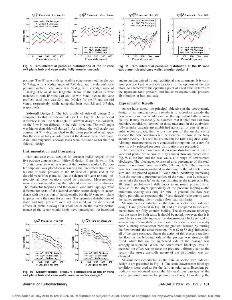
passage. The IP vane midspan trailing edge mean metal angle was65.7 deg, with a wedge angle of 7.96 deg, and the deswirl vanepressure surface metal angle was 58 deg, with a wedge angle of13.8 deg. The axial and tangential leans of the sidewalls werematched at both IP vane exit and deswirl vane inlet to the vaneprofiles: axial lean was 22.0 and 0.0 deg for the IP and deswirlvanes, respectively, while tangential lean was 3.8 and 6.7 deg,respectively.

Sidewall Design 2. The hub profile of sidewall design 2 iscompared to that of sidewall design 1 in Fig. 8. The principaldifference is that the wall angle of sidewall design 2 is constant,so the flow is not diffused in the axial direction. The wall anglewas higher than sidewall design 1. At midspan the wall angle wasconstant at 71.9 deg, matched to the mean predicted whirl angle�for the case of fully annular flow� at the deswirl vane inlet plane.Axial and tangential sidewall leans were the same as for the firstsidewall design.

Instrumentation and ProcessingHub and case cross sections �at constant radial height� of the

five-passage annular sector �sidewall design 1� are shown in Fig.7. Static pressure was measured at the positions marked. Particu-lar emphasis was placed on measuring the circumferential distri-butions of static pressure at the IP vane exit plane and at thedeswirl vane inlet plane, so that the degree of �vane-to-vane� pe-riodicity at these locations could be quantified. Measurementswere also conducted along the hub and case walls at midsector.The midsector tappings and the deswirl vane inlet tappings weredifferent for tests of the second annular sector design, in accor-dance with the position of the sidewalls, but the IP vane exit-planetappings were the same for all tests. The spanwise distributions ofstatic and total pressure were not measured, as the detrimentaleffects of probe blockage �at small scale� on the overall perfor-mance of the sector would likely have outweighed the increased

understanding gained through additional measurements. It is com-mon practice �and acceptable practice in the opinion of the au-thors� to characterize the operating point of a test vane in terms ofthe upstream total pressure and the downstream static pressuredistributions at hub and case.

Experimental ResultsAs we have noted, the principal objective in the aerodynamic

design of an annular sector cascade is to reproduce exactly theflow conditions that would exist in the equivalent fully annularfacility. It may reasonably be assumed that if inlet and exit flowboundary conditions identical to those measured in the equivalentfully annular cascade are established across all or part of an an-nular sector cascade, then across this part of the annular sectorcascade the flow conditions will be identical to those in the fullyannular facility. This will be assumed in the following discussion.Although measurements were conducted throughout the sector, forbrevity, only selected pressure distributions are presented.

The measured circumferential pressure distributions at the IPvane exit plane for the case of fully annular flow are presented inFig. 9, at the hub and the case walls, at a range of downstreamblockages. The blockages, expressed as a percentage of the totaldeswirl vane throat area, were 0%, 5%, and 10%. The pressureshave been nondimensionalized by dividing by the inlet total pres-sure and are plotted against IP vane pitch, positively increasingfrom the suction to pressure surface of the vane—that is, measure-ments take the same left to right positioning as the tappings in Fig.10. Small pitch-to-pitch differences in measured pressure arisebecause of the slight aperiodicity of the pressure tappings—theminimum spacing was only 4.5 mm. In general, the flow washighly periodic, as expected: the IP and deswirl vane counts werethe same, ensuring pitch-to-pitch flow path similarity.

Measurements conducted in the annular sector with sidewalldesign 1 are presented in Fig. 10, and are compared to measure-ments from the fully annular facility. The downstream blockagewas the same for both tests. It should be noted, however, that it ispossible to smoothly increase the downstream blockage, and soachieve any intermediate pressure ratio. Periodicity was markedlypoor: a strong cross-sector pressure gradient �caused by turningthe flow towards the axial direction, from 67 to 58 deg� influencedall of the vane passages. Under the action of this pressure gradientthe flow on the left-hand side of the passage was strongly dif-fused, while that on the right-hand side of the passage wasstrongly accelerated. When the downstream blockage was in-creased, the effect was to raise the pressure uniformly across thesector—the strong aperiodic nature of the distribution was un-changed.

Measurements conducted in the annular sector with sidewalldesign 2 are presented in Fig. 11. The same downstream blockageconditions were used as for the fully annular tests. Excellent pe-riodicity was obtained across the left-hand four passages of thesector �minimal cross-sector pressure gradients�. Considering the

Fig. 9 Circumferential pressure distributions at the IP vaneexit plane hub and case walls: fully annular cascade

Fig. 10 Circumferential pressure distributions at the IP vaneexit plane hub and case walls: annular sector design 1

Fig. 11 Circumferential pressure distribution at the IP vaneexit plane hub and case walls: annular design 2



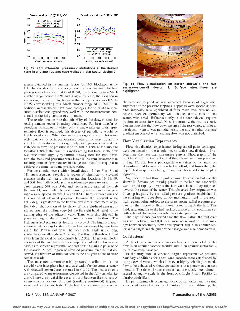
results obtained in the annular sector for 10% blockage: at thehub, the variation in midpassage pressure ratio between the fourpassages was between 0.540 and 0.570, corresponding to a Machnumber range between 0.98 and 0.94; at the case, the variation inmidpassage pressure ratio between the four passages was 0.660–0.675, corresponding to a Mach number range of 0.79–0.77. Inaddition, across the four left-hand passages, the form of the mea-sured distributions agreed very well with the measurements con-ducted in the fully annular environment.

The results demonstrate the suitability of the deswirl vane forsetting annular sector boundary conditions. For heat transfer oraerodynamic studies in which only a single passage with repre-sentative flow is required, this degree of periodicity would behighly satisfactory. When the central passage �for example� is ex-actly matched to the target operating point of the vane, by adjust-ing the downstream blockage, adjacent passages would bematched in terms of pressure ratio to within 1.9% at the hub andto within 0.8% at the case. It is worth noting that because the flowwas accelerated slightly by turning it away from the axial direc-tion, the measured pressures were lower in the annular sector thanfor fully annular flow. Greater blockage was therefore required toachieve the same test vane pressure ratio.

For the annular sector with sidewall design 2 �see Figs. 8 and11�, measurements revealed a region of significantly elevatedpressure in the right-hand passage �tapping locations 10, 11, 49,and 50�. For 10% blockage, the midpassage pressure ratio at thecase �tapping 50� was 0.76, and the pressure ratio at the hub�tapping 11� was 0.68. The corresponding measurements in pas-sage 4 were approximately 0.66 and 0.54. There are two causes ofthis region of elevated pressure. Because the sidewall angle�71.9 deg� is greater than the IP vane pressure surface metal angle�69.7 deg� the location of the throat of the right-hand passage ismoved from the trailing edge �of the far right-hand vane� to thetrailing edge of the adjacent vane. Thus, with this sidewall inplace, tapping numbers 11 and 50 are upstream of the throat. Thehigh measured pressure is therefore expected. The high pressuresmeasured at tapping locations 10 and 49 are caused by overturn-ing of the IP vane exit flow. The mean metal angle is 65.7 deg,while the sidewall angle is 71.9 deg. The flow is therefore turnedaway from the axial by approximately 6.2 deg. The general modusoperandi of the annular sector technique �or indeed the linear cas-cade� is to achieve representative conditions in a single passage ofthe cascade. A local region of elevated pressure, such as that ob-served, is therefore of little concern to the designer of the annularsector cascade.

The measured circumferential pressure distributions at thedeswirl vane inlet plane hub and case walls for the annular sectorwith sidewall design 2 are presented in Fig. 12. The measurementsare compared to measurements conducted in the fully annular fa-cility. There are slight differences in form between the two sets ofmeasurements because different �similarly positioned� tappingswere used for the two tests. At the hub, the pressure profile is not

characteristic stepped, as was expected, because of slight mis-alignment of the pressure tappings. Tappings were spaced at half-pitch intervals, so a significant shift in mean level was not ex-pected. Excellent periodicity was achieved across most of thesector, with small differences only in the near-sidewall regions�regions of secondary flow�. Most importantly, the results clearlydemonstrate that the flow downstream of the test vanes, at inlet tothe deswirl vanes, was periodic. Also, the strong radial pressuregradient associated with swirling flow was not disturbed.

Flow Visualization ExperimentsFlow-visualization experiments �using an oil-paint technique�

were conducted �in the annular sector with sidewall design 2� todetermine the near-wall streamline pattern. Photographs of theright-hand wall of the sector, and the hub endwall, are presentedin Fig. 13. The lower photograph was taken of the same oilstreamlines, but from a position to the left of, and lower than, theupper photograph. For clarity, arrows have been added to the pho-tographs.

Significant radial flow migration was observed on both of thesidewalls. Streamlines initially parallel to the hub and case wallswere turned rapidly towards the hub wall, hence, they migratedtowards the center of the sector. This observed flow migration wasdriven principally by the radial pressure gradient established inthe swirling exit-duct flow. Lower momentum fluid in the near-wall region, being subject to the same strong radial pressure gra-dient as the midsector fluid, is overturned towards the hub. Thisfluid, migrating on to the hub surface, displaces the streamlines atboth sides of the sector towards the center passages.

The experiments confirmed that the flow within the exit ductwas well behaved, and that there were no separations. The anal-ogy between secondary flow development within an annular sec-tor and a single nozzle guide vane passage was also demonstrated.

ConclusionsA direct aerodynamic comparison has been conducted of the

flow in an annular cascade facility, and in an annular sector facil-ity of five vane passages.

In the fully annular cascade, engine representative pressureboundary conditions for a test vane cascade were established byusing deswirl vanes, which allow even highly whirling transonicflow to be exhausted without unsteadiness to a plenum at constantpressure. The deswirl vane concept has previously been demon-strated at engine scale in the Isentropic Light Piston Facility atFarnborough �8,9�.

By partitioning a five-passage sector of test vanes, and by usinga sector of deswirl vanes for downstream flow conditioning, the

Fig. 12 Circumferential pressure distributions at the deswirlvane inlet plane hub and case walls: annular sector design 2

Fig. 13 Flow visualization on sector sidewalls and hubsurface—sidewall design 2. Surface streamlines arehighlighted.



applicability of the deswirl technology to the annular sectorboundary condition problem was investigated. Excellent periodic-ity was obtained across most of the sector, and it was demon-strated that by using the deswirl vane technology, the radial pres-sure gradient downstream of the test vanes �established in theswirling exit flow� was not disturbed. The technique represents asignificant improvement over previous methods, and it is the firsttime that correct annular sector boundary conditions have beenachieved to such satisfaction. Using the deswirl system, it is alsopossible to tune the mean downstream pressure, and thus, theoperating point of the test vane. The technique is equally suited tothe testing of highly three-dimensional vane profiles. If largespanwise variations in exit whirl angle exist, these can be re-moved gradually by correct sidewall contouring. The deswirl sys-tem therefore presents a means by which the problems associatedwith establishing annular sector boundary conditions may be re-solved, allowing designers to exploit the obvious advantages ofthe annular sector cascade technique: the reduced cost of bothfacility manufacture and operation, and the use of engine parts inplace of two-dimensional counterparts.

For investigations of surface heat transfer rate on modern high-pressure turbine vanes/blades, components that are, in general,highly three-dimensional and which have very complicated cool-ing systems, it is becoming unsatisfactory to use anything but theactual engine components. For these critical components, the ge-ometry, film-cooling flows, and pressure gradients must all besimultaneously correct for the results of experimental studies to beregarded as truly engine representative. Despite their importance,relatively few such investigations are performed. This is because

the costs are prohibitively high. The new annular sector techniquepresented in this paper provides a means by which engine-representative flow conditions can be established using only asmall number of vanes and at a cost commensurate with the re-search environment.

References�1� Hirsch, H., ed., 1993, “Advance Methods for Cascade Testing,” AGARD-AG-

328.�2� Gladden, H. J., and Gauntner, J. W., 1975, “Experimental Verification of Film-

Cooling Concepts on a Turbine Vane,” ASME Paper No. 75-WA/GT-21.�3� Radeklint, U. R., and Hjalmarsson, C. S., 1998, “A New Test Facility for

Testing of Cooled Gas Turbine Components,” ASME Paper No. 98-GT-557.�4� Wiers, S. H., and Fransson, T. H., 2000, “Experimental Investigation of the

Periodicity in a Sector of an Annular Turbine Cascade,” 15th Bi-Annular Sym-posium on Measuring Techniques in Transonic and Supersonic Flow in Cas-cades and Turbomachines, Firenze, Italy, 21–22.

�5� Vogt, D. M., and Fransson, T. H., 2002, “A New Turbine Cascade for Aero-mechanical Testing,” Presented at the 16th Symposium on Measuring Tech-niques in Transonic and Supersonic Flow in Cascades and Turbomachines,Cambridge, UK, September.

�6� Hodson, H. P., and Dominy, R. G., 1993, “Annular and Rotating Cascades,”Chap. 3, AGARD-AG-328.

�7� Squire, L. C., 1986, “Effects of Probe Supports on Measurements in SteamTurbines,” ASME Paper No. 86-GT-213.

�8� Povey, T., Chana, K. S., Oldfield, M. L. G., Jones, T. V., and Owen, A. K.,2001, “The Design and Performance of a Transonic Flow Deswirling System,”Proceedings of the IMechE Advances of CFD in Fluid Machinery DesignSeminar, London, June 13.

�9� Povey, T., Chana, K. S., Jones, T. V., and Oldfield, M. L. G., 2003, “TheDesign and Performance of a Transonic Flow Deswirling System—An Appli-cation of Current CFD Design Techniques Tested Against Model and Full-Scale Experiments,” Advances of CFD in Fluid Machinery Design, R. L. El-der, A. Tourlidakis, and M. K. Yates, eds., IMechE Professional Engineering,London, pp. 65–94.



Daniel Crichton

Liping Xu

Cesare A. Hall

Whittle Laboratory,Department of Engineering,

Madingley Road,Cambridge, CB3 0DY, United Kingdom

Preliminary Fan Designfor a Silent AircraftPreliminary fan design for a functionally silent aircraft has been performed with noisereduction as the primary goal. For such an aircraft the fan design must, in addition todelivering low cruise fuel burn, enable low jet and fan source noise during takeoff. Thisrequires the fan to be operating at low pressure ratio and high efficiency during takeoffand, for conditions where the relative tip Mach number onto the fan is supersonic,ensuring the primary shock structure is ingested into the blade passage. To meet theserequirements, flyover and cruise flow coefficients are matched using a variable areanozzle at the same time as delivering low takeoff FPR. This places the sideline operatingpoint near the shoulder of the characteristic and fixes the top of climb and cruise fanpressure ratios. For a 4-engine, 250 pax, 4000 nm silent aircraft this approach leads toa top of climb FPR of 1.45, requiring a 39% increase in nozzle area at takeoff. A fan rotorhas been designed for this cycle with 20 blades, low tip loading during takeoff, and a350 m/s top of climb tip speed. �DOI: 10.1115/1.2372779�

IntroductionWhile noise from civil aircraft has reduced significantly over

the last 20 years, the downward trend is levelling off and, withinthe UK, predicted increases in aircraft movements are expected tolead to increasing aircraft noise exposure around airports in thefuture �1,2�. The ACARE2020 goals �3� that include efficiencyand emissions targets in addition to a 50% reduction in perceivednoise relative to 2000 technology levels are proving to be ex-tremely challenging. It has been argued that meeting these targetswill require revolution rather than evolution in airframe and en-gine concepts �4�.

The Silent Aircraft Initiative 2025 goal of a reduction in air-frame and engine noise sources to a point where they are imper-ceptible outside of the airport boundary in an urban environment�see Fig. 1� is considerably more challenging than the ACAREnoise target. By taking noise reduction as the primary designdriver alongside mission requirements and fuel burn, the intentionis to explore innovative solutions applicable within the ACARE-2020 time frame and beyond. To this end, in this paper, noisereduction requirements drive the selection of key design values.

For the purposes of this study the SAI noise goal has beenexpressed as a peak dBA value that should not be exceeded out-side of a typical airport boundary. A peak dBA value was used asit can be linked to both World Health Organization guidelines oncommunity noise and data on average traffic noise levels in atypical urban area �5,6�. In addition, unlike DNL or EPNdB itdoes not require prior knowledge of flight profiles and �for DNL�traffic patterns.

Previous work on the installation and configuration of enginesfor a silent aircraft has pointed to an embedded engine configura-tion on top of an all-lifting body aircraft as a promising conceptfor ultralow noise �7�. Embedding the engines shields a largeamount of forward propagating noise and enables longer ductingfor acoustic treatment �8�. Ingesting and reenergizing some of thesuction surface boundary layer has the potential to reduce aircraftdrag enabling, for an ultralow noise aircraft, lower takeoff jetvelocity. From a system perspective, increases in fan diameter donot require increases in landing gear length. In addition, the rela-tionship between fan diameter and nacelle drag is altered, leading

to the point at which minimum fuel burn is reached occurring at alarger fan diameter and lower jet stagnation pressure �7�. Theinstallation does though introduce a range of problems not found,or less critical, in traditional underwing designs. Even withoutboundary layer ingestion, pressure recovery of the inlet is likely tobe lower and distortion at the fan face higher compared to poddedengines. Adding boundary layer ingestion to this can lead to sig-nificant inlet distortion at the fan face during cruise �9�. Safety andcertification concerns including survival of turbine disk failureand impact of an engine out on airframe and adjacent engineperformance require further consideration during the design pro-cess.

While previous work on quiet engine design has tended to beless far-reaching in terms of noise target and more constrained inthat standard installation and flight operations were specified, sev-eral conclusions are applicable to the silent aircraft project. With alower fan pressure ratio �FPR� leading to lower jet noise andgenerally lower source noise, the tradeoff between noise reductionand increasing fuel burn is critical. Gliebe and Janardan �10� in-vestigated direct drive and geared fans for large twin engine air-craft with the aim of achieving 5–10 EPN dB reduction relativeto FAR36 stage 3 at each measuring station. They concluded thattop of climb FPR in the range 1.4 to 1.55 was optimal for lownoise with acceptable weight and direct operating cost �DOC�penalties. More recent work by Daggett et al. �11� with a 2015time frame aimed for ultrahigh efficiency with a noise level20 EPNdB cumulative below stage 3. For a single �geared� fan itwas found that a FPR of 1.45 was optimal in terms of DOC withlower FPR designs leading to increased weight and drag offsettingSFC improvements. As an ultralow noise concept, Dittmar hasproposed a two stage fan of design overall pressure ratio 1.15�12,13�. This gives low jet and fan noise but at the expense of avery large installation requirement leading to poor cruise perfor-mance.

To meet the silent aircraft noise target and have competitivefuel burn, a turbofan engine concept needs to operate with a fanpressure ratio in the range proposed by Dittmar at takeoff for lowjet noise and in the range proposed by Gliebe and Daggett at topof climb for low fuel consumption. This requires a variable cycleengine design as described in Ref. �7�. Furthermore, low fansource noise is required at takeoff and in this paper we demon-strate how this can also be achieved with the use of a variable areaexhaust nozzle. A design approach is presented that determines thefan rotor design parameters and the off-design operation needed tosatisfy all the noise requirements while maintaining high effi-

Contributed by the International Gas Turbine Institute �IGTI� of ASME for pub-lication in the JOURNAL OF TURBOMACHINERY. Manuscript received October 1, 2005;final manuscript received February 1, 2006. IGTI Review Chair: R. S. Abhari. Paperpresented at the ASME Turbo Expo 2006: Barcelona, Spain, May 8–11, 2006, PaperNo. GT2006-90564.



ciency. A rotor design and the corresponding characteristic arepresented and the resulting requirements on future outlet guidevanes are discussed. With the aerothermal and acoustic implica-tions of using a variable area nozzle worthy of detailed attention,the mechanical design of such a nozzle, while critical, has beenleft to a later stage.

Engine CycleWhile a considerable volume of work has been published in

recent years on lowering jet noise through lobes, tabs, or otherforms of jet shaping, a significant reduction in jet noise whilemaintaining thrust requires an increased jet area and reduced jetvelocity. To avoid suboptimal cruise performance through in-creased engine weight and drag, it is desirable to minimize anyrequired jet velocity reductions during takeoff relative to currenttrends. To this end, optimization of the aircraft takeoff profile tominimize the required jet area at takeoff has been performed bythe authors �14� using the Stone jet noise model �15� and ESDUatmospheric corrections �16,17� to predict noise on the ground.

For a specified jet area the aircraft accelerates until rotationspeed is reached and then climbs as steeply as possible at constantspeed without exceeding the jet noise target outside of the airportboundary at any time. The jet area is then iteratively modified andthe takeoff reflown until all operating requirements are met.

Figure 2 shows resulting takeoff profiles for a 4-engine250 pax, 4000 nm aircraft �described further in Table 1� achievedfrom the baseline SAI airport under sea level ISA+12 K condi-tions. The runway length used was 10 000 ft and the airportboundary was set at a sideline distance of 450 m and a flyoverdistance of 1000 m from the runway. The sideline distancematches the ICAO certification value, but the flyover position

used here is different from the certification flyover position �4048rather than 6500 m after brakes off� �18� so as to be more closelyaligned to the SAI goal. Airport and atmospheric parameters wereselected to be more arduous than the majority of conditions asilent aircraft would be required to operate under with the atmo-spheric conditions covering 99% of operating hours at LondonHeathrow and the runway relatively short. A range of takeoff con-ditions likely to only be experienced rarely or at noise uncon-strained airports have been considered during the design and canbe achieved by relaxing the noise target.

Within Fig. 2, four different departure profiles are shown. Thesolid line is the optimized departure that meets all takeoff require-ments with the minimum jet area. If the area is decreased by 10%and the same noise target met, then the lower dashed departureprofiles is achieved. The reduced jet area leads to reduced thrustlimiting the acceleration and climb rate. As the aircraft nears theairport boundary, the angle of climb has to reduce below thatrequired to comply with engine-out safety requirements in orderto not exceed the noise target. Conversely, if the area is increased10% then all operational requirements are met, but achieving thetop of climb performance will be harder. The dotted line repre-sents a successful takeoff without allowing the angle of climb toreduce as the aircraft crosses the airport boundary. This simpledeparture profile requires a 33% increase in jet area relative to theoptimized profile in order to meet the same noise target. The mini-mum regulated cutback height of 800 ft �19,20� is not enforced asthe entire takeoff profile is low noise optimized with a continuousvariation in thrust.

Fig. 3 shows how the required jet area varies with noise target

Fig. 1 Reduction in thrust corrected aircraft noise level overtime

Fig. 2 Takeoff profile optimization for jet noise outside airportboundary „10 000 ft runway, airport boundary 450 m at the side-line and 1000 m from the end of the runway at flyover, sea levelISA+12 K conditions…

Table 1 250 pax, 400 nm aircraft parameters for 2 engine pod-ded and 4 engine embedded variants

Variant Sideline FlyoverTop ofclimb

Start ofcruise

Altitude - 190 m 210 m 12 192 m 12 192 mConditions - ISA+12 K ISA+10 K ISAVelocity - 85 m/s Mach 0.8 Mach 0.8Angle ofclimb

2 eng7.5 deg

4.1 deg0.33 deg 0 deg

4 eng 1.9 degPRIN 2 eng 0.995

4 eng 0.98 0.96PROUT 2 eng 1.0

4 eng 0.98�p

- 92%Net thrust 2 eng

304.0 kN230.4 kN

75.2 kN 66.8 kN4 eng 173.2 kN

Fig. 3 Reduction in the required jet area achieved through op-timization of the takeoff profile for different peak jet noiserequirements



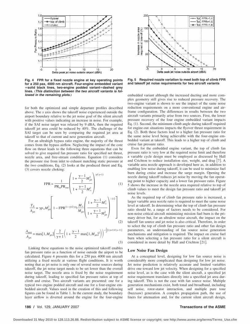
for both the optimized and simple departure profiles describedabove. The x axis shows the takeoff noise experienced outside theairport boundary relative to the jet noise goal of the silent aircraftwith positive values indicating an increase in noise. For example,if the SAI noise target was relaxed by 9 dBA, then the requiredtakeoff jet area could be reduced by 40%. The challenge of theSAI target can be seen by comparing the required jet area attakeoff to that of current and next generation aircraft.

For an ultrahigh bypass ratio engine, the majority of the thrustcomes from the bypass airflow. Neglecting the impact of the coreflow on thrust leads to the following three equations that can besolved to give required fan pressure ratio for specified net thrust,nozzle area, and free-stream conditions. Equation �1� considersthe pressure rise from inlet to exhaust matching static pressure atthe two conditions, Eq. �2� looks at the produced thrust and Eq.�3� covers nozzle choking:

FPR =1

PRinPRout� 1 +� − 1

2Mjet

2

1 +� − 1

2M�

2 ��/��−1�

�1�

TN

Ajet= �p�Mjet

2 �1 − FPR�1−��/2��pM�

Mjet� 1 +� − 1

2M�

2

1 +� − 1

2Mjet

2 �−1/2

��2�

Anoz

Ajet= max�1,Mjet� 2

� + 11 +

� − 1

2max�1,Mjet�2− 1

2��+1�/��−1��

�3�Linking these equations to the noise optimized takeoff enables

fan pressure ratio as a function of noise outside the airport to becalculated. Figure 4 presents this for a 250 pax 4000 nm aircraftutilizing a fixed nozzle at various flight conditions. It is worthnoting that as jet noise is only one of several noise sources duringtakeoff, the jet noise target needs to be set lower than the overallnoise target. The nozzle area is fixed by the noise requirementduring takeoff, leading to specified fan pressure ratios at top ofclimb and cruise. Two aircraft variants are presented: one for atypical two engine podded aircraft and one for a four-engine em-bedded aircraft. Values used in the creation of this and followingfigures can be found in Table 1. In the current study, the boundarylayer airflow is diverted around the engine for the four-engine

embedded variant although the increased ducting and more com-plex geometry still gives rise to reduced pressure recovery. Thetwo-engine variant is shown to see the impact of the same noisereduction requirements on a more conventional engine and air-frame configuration. The differences in results between the twoaircraft variants primarily arise from two sources. First, the lowerpressure recovery of the four engine embedded variant impactsEq. �1�. Second, the minimum climb angle during takeoff requiredfor engine-out situations impacts the flyover thrust requirement inEq. �2�. Both these factors lead to a higher fan pressure ratio forthe same noise level being achievable with the four-engine em-bedded variant at takeoff. This leads to a higher top of climb andcruise fan pressure ratio.

Even for the embedded engine variant, the top of climb fanpressure ratio is very low at the required noise limit and thereforea variable cycle design must be employed as discussed by Halland Crichton to reduce installation size, weight, and drag �7�. Avariable area nozzle approach is developed here as, in addition toenabling low noise during takeoff, it can be used to minimize fuelburn during cruise and increase the surge margin. Opening thenozzle during takeoff reduces jet noise by moving the fan operat-ing point to higher capacity and a lower fan pressure ratio. Figure5 shows the increase in the nozzle area required relative to top ofclimb values to meet the design fan pressure ratio and takeoff jetnoise levels.

As the required top of climb fan pressure ratio is increased, alarger variable area nozzle ratio is required to meet the same noiselevel at takeoff. In determining what the top of climb fan pressureratio should be, a range of factors needs to be considered. Fornon-noise critical aircraft minimizing mission fuel burn is the pri-mary driver but, for an ultralow noise aircraft, the impact on thetakeoff fan source and jet noise is also critical. Therefore, in orderto select the top of climb fan pressure ratio and other fan designparameters, an understanding of fan source noise generationmechanisms and mitigation is required. The impact on cruise fuelburn when selecting a fan pressure ratio for a silent aircraft isconsidered in more detail by Hall and Crichton �21�.

Low Noise Fan DesignAt a conceptual level, designing for low fan source noise is

considerably more complicated than designing for low jet noise.Jet noise prediction is relatively accurate and limited variablesdrive one toward low jet velocity. When designing for a specifiednoise level, as is the case with the silent aircraft, a specified jetnoise requirement translates directly into a specified jet area dur-ing takeoff. This is not the case with fan source noise. Multiplegeneration mechanisms exist, both tonal and broadband, includingself noise, rotor-stator interaction, and multiple pure tone�buzzsaw� generation. A complex propagation path, the use ofliners for attenuation and, for the current silent aircraft design,

Fig. 4 FPR for a fixed nozzle engine at key operating pointsfor a 250 pax, 4000 nm aircraft. Four-engine embedded variant�solid black lines, two-engine podded variant�dashed greylines. „This distinction between the two aircraft variants is fol-lowed in the remaining plots.…

Fig. 5 Required nozzle variation to meet both top of climb FPRand takeoff jet noise requirements for two aircraft variants



shielding of forward propagating noise from the airframe, furthercomplicate the problem. Publicly available noise prediction capa-bilities are less mature, especially in relation to broadband noisemaking designing for an absolute noise level hard. This is espe-cially true for an engine using a variable area nozzle as the fanoperating line during takeoff is markedly different from conven-tional civil engines on which current correlations are based.

For a preliminary fan design, the authors have therefore usedavailable results, predictions, and correlations to guide the processand have not attempted to design for a specified noise level at thisstage. Complementary work on the tradeoffs in liner length andinlet design for embedded engines is currently being undertakenwithin the silent aircraft project. Once the result of this work isavailable, state of the art methods to predict source noise andresulting noise on the ground will be used. While in the currentwork only rotor design is performed, the impact of this design onstator generated noise is considered.

Previous research has shown that increased nozzle area can leadto reduced fan noise for a given thrust. In the 1970s Woodwardand Lucas �22� tested a 1.25 pressure ratio fan with area increasesup to 20% of the design area. Reductions in noise level at alloperating speeds were witnessed alongside increases in efficiency.Ginder and Newby �23� developed a broadband noise predictionmodel based on this and other work that correlated fan noise toinflow incidence. More recently, Hughes et al. �24� have shownthat small increases in nozzle area �up to 12.9%� can give thrustincreases and reduced broadband noise with modern wide chordfan designs. Work on the same rig �25� with two rotor designs hasshown, at subsonic fan tip speeds, a link between noise generationand wake severity.

Correlations such as those based on the work of Heidmann�26�, although not suitable for the direct application to enginesworking well away from normal working lines, provide furtherinsight into suitable approaches to noise reduction. The ESDU fanand compressor prediction code �27� based on Heidmann presentsbroadband and tonal noise sources in the form of Eq. �4� withsome variation for the different sources. RSS is the rotor-statorspacing and BPF the blade passing frequency.

SPL�f� = 20 log10��T0� + 10 log10�m� + F1�Mrel� + F2�RSS�

+ F3�� + F4�f/BPF� + C �4�

In terms of cycle and fan rotor preliminary design, the variablesthat can be targeted are the temperature rise across the fan, themass flow rate, and the relative flow Mach number. With fanpressure ratio and mass flow rate set by the requirement for lowjet noise, high fan efficiency is required to minimize the tempera-ture rise. This correlates well with the work of Ginder and Newbyas efficiency is closely linked to the incidence angle onto the rotorand, for a normal engine working line during takeoff, reducedincidence equals increased efficiency.

While the traditional 50 log�tip speed� correlation, used in �23�for example, would suggest reducing fan tip speed to reducenoise, this is not always the case. A second fan design as part ofthe NASA Advance Subsonic Technology project was found to belouder than its predecessor, despite having a reduced tip speed.Topol et al. �28� found this to be primarily due to increased broad-band noise from increased fan tip turbulence impacting the stator.Included within this work is a simple formulation covering broad-band noise generation �Eq. �5�� in which C is the absolute velocityonto the stator, V0 is the turbulent velocity, and NV is the numberof Outlet Guide Vanes �OGVs�.

Sound Power � 10 log�C3V02NV� �5�

Reducing rotor loading and the absolute flow velocity onto theOGVs, especially at the tip, is therefore required during takeoff.While increasing, the nozzle area will increase fan tip speed forthe same thrust; the high cruise altitude and low design point fanpressure ratio lead to excess thrust at a low flight speed �reducingthe fan pressure ratio increases the cruise ram drag more than the

takeoff ram drag�. In addition a four-engine design requires areduced climb angle compared to a two-engine design. The fancan therefore operate at part speed during takeoff, resulting in lowrotor loading at the tip and lower flow velocity onto the OGVs.

With the rapid onset of multiple pure tone noise at supersonicrelative tip Mach numbers, maintaining subsonic tip velocity at alltimes during takeoff is desirable. As discussed later, achieving thisfor the entire takeoff leads to reduced cruise performance andtherefore alternative mitigation strategies must be considered. Asthe nozzle area is increased the fan backpressure is reduced, and,for a fan operating with supersonic relative inlet flow, the primaryshock structure is ingested into the blade passage, leading to chok-ing. A weaker bow shock detached from the leading edge stillpropagates upstream, but a considerable reduction in MPT noise ispredicted for this situation �29�. For fans working with a fixednozzle area, this effect is generally only seen at high fan speed,where the shock is just ingested at the tip for peak efficiency. Thismay explain the more rapid than expected reduction in MPT noiseat higher Mach numbers seen by Prasad and Prasad �30�, whocompared their results to the analysis of Morfey and Fisher �31�.In their analysis, Morfey and Fisher modeled the flow as havingdetached normal shocks for all conditions.

To summarize, for low fan source noise while maintaining lowjet noise, high efficiency and low tip loading is required during theentire takeoff procedure. To minimize multiple pure tone genera-tion, when the flow onto the rotor tip is supersonic the primaryshock structure should be ingested into the blade passage. Theserequirements are now considered in the selection of fan rotor de-sign parameters.

Selection of Fan Rotor Design ParametersA variable area nozzle enables the fan to be operated at any

position on its characteristic for a specified thrust. During cruisethe nozzle can be set for minimum fuel burn, for hot and highoperations the nozzle can be closed to increase available thrustand, during takeoff the nozzle can be set to minimize noise.

With the nozzle setting impacting both fan and jet noise thesame nozzle position needs to meet the requirements of bothsources. This requires the fan pressure ratio being at a specifiedlevel for low jet noise and the fan operating at an efficient positionfor low fan noise. The aircraft is as close as it gets to groundoutside the airport boundary at the flyover position and, as jetnoise reduces more rapidly than fan noise when the engine isthrottled back, this position is critical. As discussed later in thissection, the relative tip flow can be set to below unity Mach num-ber at this position and therefore high fan efficiency is the mainrequirement. At the sideline position the subsonic tip Mach num-ber cannot be maintained and therefore while high efficiency isstill important, any primary shock structures must be ingested tominimize MPT noise. This requires operating near the shoulder ofthe fan characteristic.

For a typical fan design, a locus of constant flow coefficient, �,tracks peak efficiency well, so ensuring both the cruise and fly-over points are at the same flow coefficient will ensure they areboth at, or close to, peak efficiency. If the nozzle is operated at afixed area during takeoff �as is assumed in the current takeoffoptimization work�, the sideline point on the fan characteristic isat a higher flow coefficient than flyover and on a higher thrustline. Setting the flyover flow coefficient to match cruise will alsotherefore place the sideline point near the fan shoulder. Perform-ing this calculation requires the use of a sample characteristicbecause the flow coefficient is a function of blade speed �see Eq.�6��. If a realistic fan map is not available, similar results can beobtained by fixing the stage loading divided by the flow coeffi-cient squared, � /�2. This is independent of blade speed but di-verges from peak efficiency at higher Mach numbers �Eq. �7��.



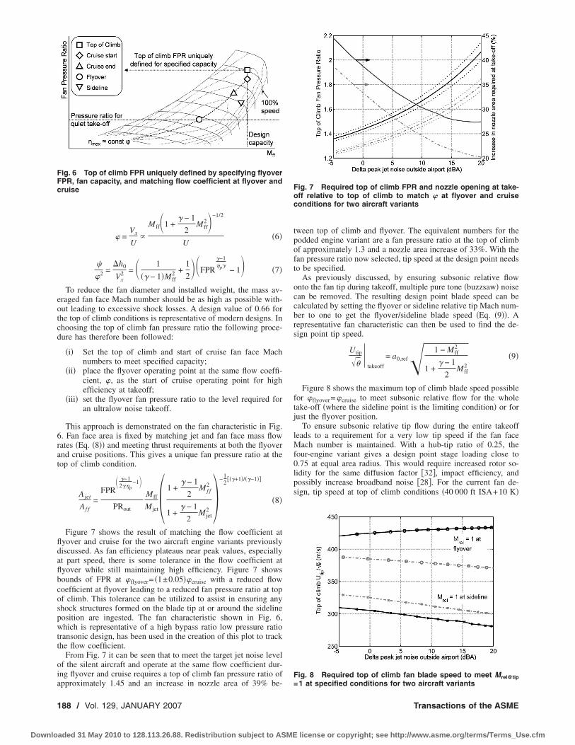
� =Vx

U�

Mff1 +� − 1

2Mff

2−1/2

U�6�

�

�2 =�h0

Vx2 = 1

�� − 1�Mff2 +

1

2FPR

�−1�p�

− 1 �7�

To reduce the fan diameter and installed weight, the mass av-eraged fan face Mach number should be as high as possible with-out leading to excessive shock losses. A design value of 0.66 forthe top of climb conditions is representative of modern designs. Inchoosing the top of climb fan pressure ratio the following proce-dure has therefore been followed:

�i� Set the top of climb and start of cruise fan face Machnumbers to meet specified capacity;

�ii� place the flyover operating point at the same flow coeffi-cient, �, as the start of cruise operating point for highefficiency at takeoff;

�iii� set the flyover fan pressure ratio to the level required foran ultralow noise takeoff.

This approach is demonstrated on the fan characteristic in Fig.6. Fan face area is fixed by matching jet and fan face mass flowrates �Eq. �8�� and meeting thrust requirements at both the flyoverand cruise positions. This gives a unique fan pressure ratio at thetop of climb condition.

Ajet

Af f=

FPR �−1

2��p−1

PRout

Mff

Mjet� 1 +� − 1

2Mf f

2

1 +� − 1

2Mjet

2 �− 1

2��+1�/��−1��

�8�

Figure 7 shows the result of matching the flow coefficient atflyover and cruise for the two aircraft engine variants previouslydiscussed. As fan efficiency plateaus near peak values, especiallyat part speed, there is some tolerance in the flow coefficient atflyover while still maintaining high efficiency. Figure 7 showsbounds of FPR at �flyover= �1±0.05��cruise with a reduced flowcoefficient at flyover leading to a reduced fan pressure ratio at topof climb. This tolerance can be utilized to assist in ensuring anyshock structures formed on the blade tip at or around the sidelineposition are ingested. The fan characteristic shown in Fig. 6,which is representative of a high bypass ratio low pressure ratiotransonic design, has been used in the creation of this plot to trackthe flow coefficient.

From Fig. 7 it can be seen that to meet the target jet noise levelof the silent aircraft and operate at the same flow coefficient dur-ing flyover and cruise requires a top of climb fan pressure ratio ofapproximately 1.45 and an increase in nozzle area of 39% be-

tween top of climb and flyover. The equivalent numbers for thepodded engine variant are a fan pressure ratio at the top of climbof approximately 1.3 and a nozzle area increase of 33%. With thefan pressure ratio now selected, tip speed at the design point needsto be specified.

As previously discussed, by ensuring subsonic relative flowonto the fan tip during takeoff, multiple pure tone �buzzsaw� noisecan be removed. The resulting design point blade speed can becalculated by setting the flyover or sideline relative tip Mach num-ber to one to get the flyover/sideline blade speed �Eq. �9��. Arepresentative fan characteristic can then be used to find the de-sign point tip speed.

�Utip

��

takeoff

= a0,ref� 1 − Mff2

1 +� − 1

2Mff

2

�9�

Figure 8 shows the maximum top of climb blade speed possiblefor �flyover=�cruise to meet subsonic relative flow for the wholetake-off �where the sideline point is the limiting condition� or forjust the flyover position.

To ensure subsonic relative tip flow during the entire takeoffleads to a requirement for a very low tip speed if the fan faceMach number is maintained. With a hub-tip ratio of 0.25, thefour-engine variant gives a design point stage loading close to0.75 at equal area radius. This would require increased rotor so-lidity for the same diffusion factor �32�, impact efficiency, andpossibly increase broadband noise �28�. For the current fan de-sign, tip speed at top of climb conditions �40 000 ft ISA+10 K�

Fig. 6 Top of climb FPR uniquely defined by specifying flyoverFPR, fan capacity, and matching flow coefficient at flyover andcruise Fig. 7 Required top of climb FPR and nozzle opening at take-

off relative to top of climb to match � at flyover and cruiseconditions for two aircraft variants

Fig. 8 Required top of climb fan blade speed to meet Mrel@tip=1 at specified conditions for two aircraft variants



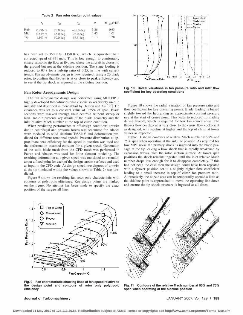
has been set to 350 m/s �1150 ft/ s�, which is equivalent to acorrected speed of 371 m/s. This is low enough to comfortablyensure subsonic tip flow at flyover, where the aircraft is closest tothe ground but not at the sideline position. The stage loading isreduced to 0.48 for a hub-tip ratio of 0.25, in line with currenttrends. Fan aerodynamic design is now required, using a 20 bladerotor, to confirm that flyover is at or close to peak efficiency andto see if the tip shock is ingested at the sideline position.

Fan Rotor Aerodynamic DesignThe fan aerodynamic design was performed using MULTIP, a

highly developed three-dimensional viscous solver widely used inindustry and described in more detail by Denton and Xu �33�. Tipclearance was set to a constant value of 0.25% of span. Bladesections were stacked through their centroid without sweep orlean. Table 2 presents key details of the blade geometry and theinlet relative Mach number at the top of climb condition.

When predicting performance at off-design conditions untwistdue to centrifugal and pressure forces was accounted for. Bladeswere modeled as solid titanium Ti6Al4V and deformation pre-dicted for different rotational speeds. Pressure distribution at ap-proximate peak efficiency for the speed in question was used andthe deformation assumed constant for a given speed. Generationof the solid blade mesh from the CFD mesh was performed inPatran and Abaqus was used for finite element modeling. Theresulting deformation at a given speed was translated to a rotationabout a fixed point for each of the design stream surfaces and usedas input to the CFD code. At design speed two degrees of untwistat the tip �included within the values shown in Table 2� was pre-dicted.

Figure 9 shows the resulting fan rotor only characteristic withcontours of polytropic efficiency. Key design points are markedon the figure. No attempt has been made to specify the exactposition of the surge/stall line.

Figure 10 shows the radial variation of fan pressure ratio andflow coefficient for key operating points. Blade loading is biasedslightly toward the hub giving an approximate constant pressurerise at the start of cruise point. This leads to reduced tip loadingduring takeoff, which is required for low fan source noise. Theflyover flow coefficient is very close to the cruise flow coefficientas designed, with sideline at higher and the top of climb at lowervalues as expected.

Figure 11 shows contours of relative Mach number at 95% and75% span when operating at the sideline position. As required forlow MPT noise the primary shock is ingested into the blade pas-sage at the tip leaving a bow shock that is rapidly weakened byexpansion waves from the rotor suction surface. At lower spanpositions the shock remains ingested until the inlet relative Machnumber drops low enough for it to disappear completely. If thishad not been the case then the design could have been repeatedwith a flyover position set to a slightly higher flow coefficientleading to a small increase in top of climb fan pressure ratio.Alternatively, the nozzle area can be temporarily opened a little asthe sideline point is approached to move the operating line downand ensure the tip shock structure is ingested at all times.

Table 2 Fan rotor design point values

r1 �1 �2 � M1,rel@DP

Hub 0.276 m 25.0 deg −26.0 deg 3.26 0.63Mid 0.689 m 45.0 deg 26.0 deg 1.45 1.01Tip 1.103 m 59.0 deg 56.5 deg 1.13 1.28

Fig. 9 Fan characteristic showing lines of fan speed relative tothe design point and contours of rotor only polytropicefficiency

Fig. 10 Radial variations in fan pressure ratio and inlet flowcoefficient for key operating conditions

Fig. 11 Contours of the relative Mach number at 95% and 75%span when operating at the sideline position



Velocity and Incidence on to OGVSWhile a variable area nozzle can be used to optimize the inci-

dence onto the fan rotor at off-design conditions, the incidenceonto the exit guide vanes moves away from optimum. Openingthe nozzle increases the axial velocity and reduces the loading,especially at the tip, resulting in reduced swirl onto the stator, asshown in Fig. 12. To cover conditions from top of climb to fly-over, the stator needs to support approximately 18 deg of swirlangle variation in the tip region with low loss. This range ofrequired incidence is challenging, but, with a low Mach number atthe tip �see Fig. 12�, just within limits of the useful incidencerange for controlled diffusion airfoils �34�. Variable pitch statorscould be employed to support the operating range but this wouldbe at the expense of additional weight and complexity.

Conclusions and Further WorkA functionally silent aircraft requires considerable jet noise re-

duction relative to conventional designs leading to a large increasein required jet area at takeoff, even when the departure profile isoptimized for low noise. This leads to a low fan pressure ratioduring takeoff and, to avoid low FPR at cruise that would lead tohigher than optimum fuel burn, a variable area nozzle is em-ployed.

This variable area nozzle, in addition to delivering the requiredFPR at cruise and takeoff, must also deliver high efficiency atboth conditions. This is because high efficiency at takeoff equateswith low fan source noise through reduced self noise and minimalwake severity onto the fan OGVs. Ingesting the primary shockstructure is required to minimize MPT noise when operating withsupersonic flow onto the fan tips. These requirements are achievedby matching the flow coefficient at flyover to that at cruise. Thismaximizes flyover efficiency and places the sideline position,where the relative tip Mach number exceeds unity, close to theshoulder of the fan characteristic. For a given capacity, the fandesign parameters are then fully constrained and top of climb andcruise fan pressure ratios fixed.

For the current 4-engine, 250 pax, 4000 nm silent aircraft con-cept, this process sets the design top of climb FPR to 1.45, requir-ing a 39% increase in nozzle area at takeoff. The FPR selected isexpected to give low fuel burn, as shown in �7� and �21�.

A 20 blade fan rotor with a hub tip ratio of 0.25 had beendesigned with the required top of climb FPR and a design bladetip speed of 350 m/s. Rotor alone efficiency is high during take-off, especially at flyover and, as required for low MPT noise, theprimary shock structure on the blades is ingested at the sidelineposition. The fan rotor tip is lightly loaded during takeoff, whichis desirable for low fan source noise.

The change in incidence onto the OGVs between top of climband flyover is considerable, especially at the tip. While literatureindicates that this is within the range of useful incidence for theflow Mach number, future work is required in this area. The OGVdesign will need to ensure low fan-stator interaction noise at take-off without impacting cruise efficiency.

Allowing the nozzle area to vary during the noise critical por-tion of the takeoff may further assist in meeting the design re-quirements and requires further investigation. This will require thenoise optimized takeoff profile development to be linked to aspecified fan operating line rather than a specified jet area. Thisoperating line can be designed to minimize incidence variationonto the OGVs and to ensure that any shock structures on theblades during takeoff are ingested.

Finally, to support the ingestion and reenergizing of airframeboundary layer airflow, further research on the design of low pres-sure ratio fans to support steady inlet distortion both from anaerodynamic and noise perspective is required.

AcknowledgmentThe authors would like to thank members of the Silent Aircraft

Initiative and Rolls Royce plc. for providing consultation and ad-vice. They would also like to acknowledge the Cambridge-MITInstitute for the financial support of this work.

Nomenclature

Latina speed of soundA area

dB decibelsdBA a-weighted decibelsDNL day night levelEPN effective perceived noise

h enthalpyM Mach numberm mass flow ratep pressure

PR pressure recoveryr radiusT temperature

TN net thrustU blade speedV velocity

Greek� ratio of specific heat capacities� fan efficiency� temperature correction, T0/T0ref solidity� flow coefficient� metal angle� stage loading

Subscripts0 stagnation conditions1 rotor leading edge2 rotor trailing edgeff fan facein inlet �free stream to fan face�jet fully expanded jet

noz nozzleout exhaust �fan exit to fully expanded�

p polytropicref referenceISA sea level

x axial� freestream

Fig. 12 Swirl and absolute Mach number onto OGVs at keyoperating points



References�1� “Air Travel—Greener by Design: The Technology Challenge,” Greener by

Design 2001.�2� “The Future of Air Transport,” Department for Transport, UK Government

2003.�3� ACARE, 2000, “European Aeronautics: A Vision for 2020,” Advisory Council

for Aeronautics Research in Europe 2000.�4� Smith, C. P., 2005, “The Environmental Challenge—Bringing Technology to

Market,” ISABE-2005–1008.�5� Berglund, B., Lindvall, T., and Schwela, D. H., 1999, “Guidelines for Com-

munity Noise,” World Health Organization.�6� “Noise Mapping England: The London Road Traffic Noise Map,” Department

for Environment, Food and Rural Affairs �Defra�, London 2004.�7� Hall, C. A., and Crichton, D., 2005, “Engine and Installation Configurations

for a Silent Aircraft,” ISABE-2005-1164.�8� Agarwal, A., and Dowling, A. P., 2005, “Low Frequency Acoustic Shielding of

Engine Noise by the Silent Aircraft Airframe,” Paper No. AIAA 2005-2996.�9� Berrier, B. L., and Allan, A. G., 2004, “Experimental and Computational

Evaluation of Flush-Mounted, S-Duct Inlets,” Paper No. AIAA 2004-0764.�10� Gliebe, P. R., and Janardan, B. A., 2003, “Ultra-High Bypass Engine Aeroa-

coustic Study,” Paper No. NASA-2003-212525.�11� Daggett, D. L., Brown, S. T., and Kawai, R. T., 2003, “Ultra-Efficient Engine

Diameter Study,” NASA CR-2003-212309.�12� Dittmar, J. H., 1998, “A Fan Concept to Meet the 2017 Noise Goals,” NASA-

TM-1998-208663.�13� Dittmar, J. H., Tweedt, D., Jeracki, R., Envia, E., Bartos, K., and Slater, J.,

2003, “A Fan Design That Meets the NASA Aeronautics Noise Goals,” NASATM-2003-212322.

�14� Crichton, D., Tan, D., and Hall, C. A., 2004, “Required Jet Area For a SilentAircraft at Take-off,” presented at the 8th ASC-CEAS Workshop, BudapestUniversity of Technology and Economics, Hungary.

�15� Stone, J. R., and Montegani, F. J., 1980, “An Improved Prediction Method forthe Noise Generated in Flight by Circular Jets,” NASA TM-81470.

�16� ESDU, 1977, “Evaluation of the Attenuation of Sound by a Uniform Atmo-sphere,” item 78002 available from www.esdu.com.

�17� ESDU, 1982, “Estimation of Lateral Attenuation of Air-to-Ground Jet or Tur-bofan Aircraft Noise in One-Third Octave Bands,” item 82027 available fromwww.esdu.com.

�18� ICAO, 1993, “Convention on International Civil Aviation—Annexe 16,” Vol.1, 3rd ed.

�19� ICAO, “PANS-OPS Volume 1 Part V: Noise Abatement Procedures.”�20� FAA, 1993, “AC 91-53A: Noise Abatement Departure Profiles.”�21� Hall, C. A., and Crichton, D., 2006, “Engine Design Studies for a Silent

Aircraft,” ASME Paper No. GT2006-90559.�22� Woodward, R. P., and Lucas, J. G., 1976, “Acoustic and Aerodynamic Perfor-

mance of a 1.83 Meter Diameter 1.25 Pressure Ratio Fan �QF-8�,” NASA TND-8130 TN D-8130.

�23� Ginder, R. B., and Newby, D. R., 1977, “An Improved Correlation for theBroadband Noise of High Speed Fans,” J. Aircr., 14, pp. 844–849.

�24� Hughes, C. E., Woodward, R. P., Podboy, G. G., and Jeracki, R. J., 2005, “TheEffect of Bypass Nozzle Exit Area on Fan Aerodynamic Performance andNoise in a Model Turbofan Simulator,” ASME Paper No. GT2005-68573.

�25� Woodward, R. P., Hughes, C. E., Jeracki, R., and Miller, C. J., 2002, “FanNoise Source Diagnostic Test—Far Field Acoustic Results,” presented at the8th AIAA/CEAS Aeroacoustics Conference & Exhibit, Breckenridge, CO.

�26� Heidmann, M. F., 1979, “Interim Prediction Method for Fan and CompressorSource Noises,” NASA TM X-71763.

�27� ESDU, 1998, “Prediction of Noise Generated by Fans and Compressors inTurbojet and Turbofan Engines,” item 98008 available from www.esdu.com.

�28� Topol, D. A., Ingram, C. L., Larkin, M. J., Roche, C. H., and Thulin, R. D.,2004, “Advanced Subsonic Technology �AST� 22-Inch Low Noise ResearchFan Rig Preliminary Design of ADP-Type Fan 3,” NASA CR-2004-212718.

�29� Xu, L., 2004, “Shockwave and Noise Abatement of Transonic Fans,” presentedat the ASME Turbo Expo: Power for Land, Sea and Air, Vienna, Austria.

�30� Prasad, A., and Prasad, D., 2005, “Unsteady Aerodynamics and Aeroacousticsof a High-Bypass Ratio Fan Stage,” ASME J. Turbomach., 127, pp. 64–75.

�31� Morfey, C. L., and Fisher, M. J., 1970, “Shock-Wave Radiation from a Super-sonic Ducted Rotor,” Aeronaut. J., 74, pp. 579–585.

�32� Wennerstrom, A. J., 2000, “Design of Highly Loaded Axial-Flow Fans andCompressors,” ISBN 0-933283-11-3.

�33� Denton, J. D., and Xu, L., 2002, “The Effects of Lean and Sweep on TransonicFan Performance,” ASME Paper No. GT-2002-30327.

�34� Hobbs, D. E., and Weingold, H. D., 1984, “Development of Controlled Diffu-sion Airfoils for Multistage Compressor Application,” ASME J. Eng. Gas Tur-bines Power, 106, pp. 271–278.



J.turbomachinery.2007.Vol.129.N1

Documents

Transcript of J.turbomachinery.2007.Vol.129.N1