JournalofVegetationScience && (2014 ... · JournalofVegetationScience&& (2014)...

Journal of Vegetation Science && (2014)

Predicting environmental gradients with fern speciescomposition in Brazilian Amazonia

Gabriela Zuquim, Hanna Tuomisto, Mirkka M. Jones, Jefferson Prado, Fernando O.G.Figueiredo, Gabriel M. Moulatlet, Flavia R.C. Costa, Carlos A. Quesada & Thaise Emilio

Keywords

Calibration methods; Edaphic characteristics;

Floristic composition; Indicator species; k-NN;

Pteridophytes; Tropical forest; Vegetation

maps; Weighted averaging

Abbreviations

db-MRT = distance-based Multivariate Tree

Regression; k-NN = k nearest-neighbours;

RMSE = Root Mean Squared Error;

WA =Weighted Averaging

Nomenclature

International Plant Name Index (IPNI) (www.

ipni.org; accessed 22 July 2013)

Received 6 August 2013

Accepted 7 January 2014

Co-ordinating Editor: Duccio Rocchini

Zuquim, G. (corresponding author,

[email protected]),

Tuomisto, H. ([email protected]),

Jones, M.M. ([email protected]):

Department of Biology, University of Turku,

FI-20014, Turku, Finland

Jones, M.M. : Ecoinformatics and Biodiversity

Group, Department of Bioscience, Aarhus

University, DK-8000, Aarhus C., Denmark

Prado, J. ([email protected]): Instituto de

Botanica, Herb�ario SP, C.P. 68041, CEP 04045-

972, S~ao Paulo, Brazil

Figueiredo, F.O.G. (nandoeco06@

gmail.com) & Emilio, T. (thaise.emilio@

gmail.com): Programa de P�os-Graduac�~ao em

Ecologia, Instituto Nacional de Pesquisas da

Amazonia (INPA/MCTI), Manaus, Brazil

Moulatlet, G.M.

([email protected]): Programa de

P�os-Graduac�~ao em Ecologia, Instituto Nacional

de Pesquisas da Amazonia (INPA/MCT),

Manaus, Brazil

Costa, F.R.C. ([email protected]) &

Quesada, C.A. ([email protected]):

Instituto Nacional de Pesquisas da Amazonia,

CP 478, 69011-970, Manaus, Brazil

Abstract

Aim: A major problem for conservation in Amazonia is that species distribution

maps are inaccurate. Consequently, conservation planning needs to be based on

other information sources such as vegetation and soil maps, which are also inac-

curate. We propose and test the use of biotic data on a common and relatively

easily inventoried group of plants to infer environmental conditions that can be

used to improvemaps of floristic patterns for plants in general.

Location: Brazilian Amazonia.

Methods: We sampled 326 plots of 250 m 9 2 m separated by distances of

1–1800 km. Terrestrial fern individuals were identified and counted. Edaphic

data were obtained from soil samples and analysed for cation concentration and

texture. Climatic data were obtained from Worldclim. We used a multivariate

regression tree to evaluate the hierarchical importance of soils and climate for

fern communities and identified significant indicator species for the resultant

classification. We then tested how well the edaphic properties of the plots could

be predicted on the basis of their floristic composition using two calibration

methods, weighted averaging and k-nearest neighbour estimation.

Results: Soil cation concentration emerged as the most important variable in

the regression tree, whereas soil textural and climatic variation played secondary

roles. Almost all the plot classes had several fern species with high indicator val-

ues for that class. Soil cation concentration was also the variable most accurately

predicted on the basis of fern community composition (R2 = 0.65–0.75 for

log-transformed data). Predictive accuracy varied little among the calibration

methods, and was not improved by the use of abundance data instead of

presence–absence data.

Conclusions: Fern species composition can be used as an indicator of soil cation

concentration, which can be expected to be relevant also for other components

of rain forests. Presence–absence data are adequate for this purpose, which

makes the collecting of additional data potentially very rapid. Comparison with

earlier studies suggests that edaphic preferences of fern species have good trans-

ferability across geographical regions within lowland Amazonia. Therefore, spe-

cies and environmental data sets already available in the Amazon region

represent a good starting point for generating better environmental and floristic

maps for conservation planning.

1Journal of Vegetation ScienceDoi: 10.1111/jvs.12174© 2014 International Association for Vegetation Science

Introduction

Understanding the spatial heterogeneity of environmental

conditions and species distributions in Amazonia is a major

challenge for conservation planning. A generally accepted

principle is that the network of conservation units should

contain adequate representation of different habitats, so as

to collectively provide living space for species adapted to

different habitats. Currently, sufficiently detailed maps

that would allow assessing whether this aim has been ful-

filled do not exist for Amazonia. The available soil and spe-

cies distributions maps are inaccurate and give an

incomplete representation of the known Amazonian

heterogeneity.

Several soil maps are available for Amazonia (RADAM-

BRASIL 1978; SOTERLAC – Dijkshoorn et al. 2005; Ques-

ada et al. 2011), but all of them are coarse-grained because

there is a general paucity of ground data. While informa-

tion on broad-scale variation in soil properties can be

extracted from such maps, this is not sufficient to take into

account the documented effects of soil variation on biotic

heterogeneity at local to landscape scales (Phillips et al.

2003; Tuomisto et al. 2003a,b,c; Costa et al. 2005; Kinupp

& Magnusson 2005; Jones et al. 2006; Ruokolainen et al.

2007; Zuquim et al. 2009a; Higgins et al. 2011). Conse-

quently, there is a general lack of knowledge of the distri-

bution of Amazonian habitat types (Emilio et al. 2010) and

species (Schulman et al. 2007a), which forces conservation

planning in Amazonia to be based on the use of more or

less unreliable surrogates (Schulman et al. 2007b).

When information on environmental gradients is

needed but measurements of environmental variables

cannot be made, biotic communities have been used as

predictors of the environmental conditions. For example,

paleo-environmental reconstructions (Birks et al. 2010)

use modern species–climatic relationships to infer past

climatic conditions according to the analogue fossil record

(ter Braak & van Dam 1989; Birks et al. 1990). The same

approach was used by Sir�en et al. (2013) to generate pre-

dictive maps of soil fertility based on fern and lycophyte

species composition in a lowland rain forest area in Ecu-

adorian Amazonia. The authors used floristic and soil data

from other parts of western Amazonia (Tuomisto et al.

2003a and H. Tuomisto unpublished data) to determine

fern and lycophyte species’ optima on a soil cation concen-

tration gradient. Then they used those optima to estimate

soil cation concentrations in their study area, where fern

and lycophyte species lists were available but direct mea-

surements of soil properties were not. Suominen et al.

(2013) recently evaluated the application of similar estima-

tion techniques for predicting chemical soil properties in

western Amazonia using species occurrence data of the

plant family Melastomataceae.

Specific taxa can also be used as indicators of particular

environments or habitat types (Ruokolainen et al. 1997,

2007; Margules et al. 2002; Tuomisto et al. 2003a; Salova-

ara et al. 2004). The use of indicator species (Noss 1990) is

an important method in conservation biology because it is

flexible (Dufrene & Legendre 1997) and conceptually

straightforward (McGeoch 1998). Well-chosen indicator

taxa can contribute significantly to a conservation strategy

by facilitating the recognition and mapping of habitats

(Noss 1990; Howard et al. 1998).

Ferns have been proposed as a suitable indicator group

in Amazonia because they are easy to observe and identify.

Several studies have documented edaphic affinities of

selected fern species in the western Amazon region in rela-

tion to either a simple classification of soil types (Tuomisto

& Poulsen 1996; Salovaara et al. 2004; C�ardenas et al.

2007), or quantitative soil gradients (Tuomisto et al. 1998,

2002; Tuomisto 2006). Some of these studies have only

reported results for a few species within selected genera,

and none has explicitly assessed the accuracy of soil prop-

erty estimates when these are based on indicator values of

the species.

In this study, we investigate the use of ferns as environ-

mental indicators in central and northern Amazonian low-

lands. First, we clarify the main environmental drivers of

fern community composition and define the environmen-

tal optima and tolerances for each species along each of

these gradients. Then we use species optima to predict

environmental variable values and test the accuracy of

these predictions. Finally, we assess whether species abun-

dance data are needed to obtain useful predictions, or

whether the more easily obtainable presence–absence data

are adequate.

Methods

Study area and sampling design

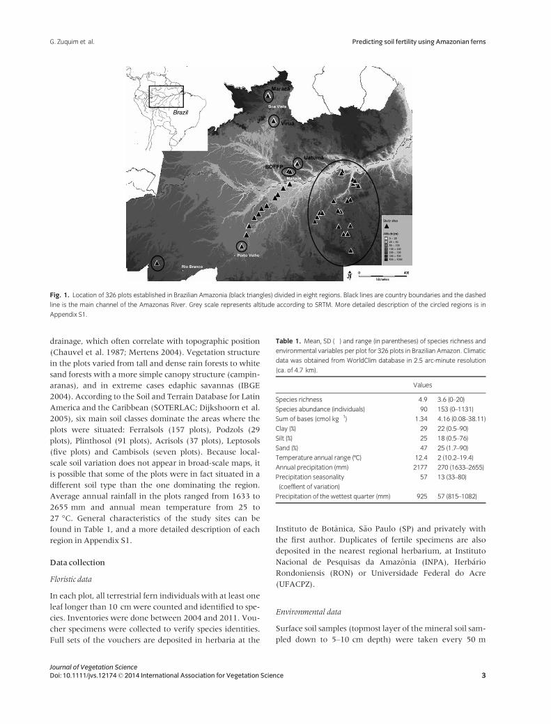
A total of 326 plots were sampled (Fig. 1). Plots were

located in Brazilian Amazonian lowlands in the states of

Acre (seven plots), Amazonas (129 plots), Par�a (101 plots),

Rondonia (30 plots) and Roraima (59 plots). All study sites

are part of the Brazilian Biodiversity Research Program

(PPBio, http://ppbio.inpa.gov.br/). Minimum distance

between plots was 1 km andmaximum ca. 1800 km. Plots

were established in private lands or in conservation units

along the highways BR-163, BR-230 (Transamazonica)

and BR-319 and in the protected areas of ReBio Uatum~a,

ESEC Marac�a, PN Viru�a, BDFFP and PE Chandless. In

every location, five to 30 plots were established according

to the RAPELD methodology (Magnusson et al. 2005).

The plots were 250 9 2 m in size and placed so that the

longer axis followed the topographic contour in order to

minimize internal heterogeneity in soil properties and

Journal of Vegetation Science2 Doi: 10.1111/jvs.12174© 2014 International Association for Vegetation Science

Predicting soil fertility using Amazonian ferns G. Zuquim et al.

drainage, which often correlate with topographic position

(Chauvel et al. 1987; Mertens 2004). Vegetation structure

in the plots varied from tall and dense rain forests to white

sand forests with a more simple canopy structure (campin-

aranas), and in extreme cases edaphic savannas (IBGE

2004). According to the Soil and Terrain Database for Latin

America and the Caribbean (SOTERLAC; Dijkshoorn et al.

2005), six main soil classes dominate the areas where the

plots were situated: Ferralsols (157 plots), Podzols (29

plots), Plinthosol (91 plots), Acrisols (37 plots), Leptosols

(five plots) and Cambisols (seven plots). Because local-

scale soil variation does not appear in broad-scale maps, it

is possible that some of the plots were in fact situated in a

different soil type than the one dominating the region.

Average annual rainfall in the plots ranged from 1633 to

2655 mm and annual mean temperature from 25 to

27 °C. General characteristics of the study sites can be

found in Table 1, and a more detailed description of each

region in Appendix S1.

Data collection

Floristic data

In each plot, all terrestrial fern individuals with at least one

leaf longer than 10 cmwere counted and identified to spe-

cies. Inventories were done between 2004 and 2011. Vou-

cher specimens were collected to verify species identities.

Full sets of the vouchers are deposited in herbaria at the

Instituto de Botanica, S~ao Paulo (SP) and privately with

the first author. Duplicates of fertile specimens are also

deposited in the nearest regional herbarium, at Instituto

Nacional de Pesquisas da Amazonia (INPA), Herb�ario

Rondoniensis (RON) or Universidade Federal do Acre

(UFACPZ).

Environmental data

Surface soil samples (topmost layer of themineral soil sam-

pled down to 5–10 cm depth) were taken every 50 m

Table 1. Mean, SD (�) and range (in parentheses) of species richness and

environmental variables per plot for 326 plots in Brazilian Amazon. Climatic

data was obtained from WorldClim database in 2.5 arc-minute resolution

(ca. of 4.7 km).

Values

Species richness 4.9 � 3.6 (0–20)

Species abundance (individuals) 90 � 153 (0–1131)

Sum of bases (cmol�kg�1) 1.34 � 4.16 (0.08–38.11)

Clay (%) 29 � 22 (0.5–90)

Silt (%) 25 � 18 (0.5–76)

Sand (%) 47 � 25 (1.7–90)

Temperature annual range (ºC) 12.4 � 2 (10.2–19.4)

Annual precipitation (mm) 2177 � 270 (1633–2655)

Precipitation seasonality

(coeffient of variation)

57 � 13 (33–80)

Precipitation of the wettest quarter (mm) 925 � 57 (815–1082)

Fig. 1. Location of 326 plots established in Brazilian Amazonia (black triangles) divided in eight regions. Black lines are country boundaries and the dashed

line is the main channel of the Amazonas River. Grey scale represents altitude according to SRTM. More detailed description of the circled regions is in

Appendix S1.


G. Zuquim et al. Predicting soil fertility using Amazonian ferns

along the long axis of each plot. The six soil samples from

the same plot were either bulked into a single composite

sample before laboratory analyses or analysed separately.

In the latter case, the obtained values were averaged to

obtain a single value for each edaphic variable for each

plot. Before laboratory analyses, the soil samples were air-

dried, cleaned of roots and other detritus and sieved

through a 2-mm mesh. Analyses included soil texture

(percentage of clay, silt and sand, using the pipette

method) and exchangeable bases (Ca, Mgwith 1N KCl and

K with Mehlich 1 standard methods for exchangeable

cations). All soil samples were analysed in the Thematic

Laboratory of Soils and Plants at INPA. Floristic data, soil

data and geographical coordinates of the plots are publicly

available at http://ppbio.inpa.gov.br/knb/style/skins/

ppbio/. The plots were georeferenced in the field using a

hand-held GPS (Garmin 12XL or Garmin 60X).

Climatic data were derived from monthly temperature

and rainfall values available in Bioclim (Hijmans et al.

2005). The variables used were annual temperature range,

annual precipitation, precipitation seasonality and precipi-

tation of the wettest quarter (Bioclim variables 7, 12, 15

and 16, respectively). The data were downloaded from

WorldClim database (http://www.worldclim.org/bioclim)

in 2.5 arc-minute resolution (about 4.7 km). The remain-

ing 15 climatic variables available in Bioclim were not

included either because they were strongly correlated with

an already selected variable, and hence provided little

additional information, or because they varied so little

within our study region that it seemed unlikely that it

would result in a floristic response. Amazonia has few cli-

mate stations, so the real resolution of the data is probably

much poorer than the nominal pixel size, and there are

known problems of data uncertainty (Hijmans et al.

2005). Nevertheless, this is currently the best available

source of temperature and rainfall data for the area. The

climatic values for each plot were extracted using the free

software DIVA-GIS (Hijmans et al. 2012).

Data analysis

Fern species that occurred in less than five plots were

excluded from all analyses, as species optima based on so

few data points were considered too unreliable. Twenty-

one plots were excluded from the analyses because they

had no fern species that reached the minimum frequency.

Analyses were therefore run on 305 plots. The sum of

exchangeable bases (concentration of Ca+Mg+K, all in

cmol�kg�1) was logarithmically transformed (base 10)

before numerical analyses. This was done because it is rea-

sonable to assume that plants react to relative rather than

absolute differences in the availability of soil nutrients, i.e.

small differences in soil cation concentration are ecologi-

cally important if the overall cation concentration is low

but inconsequential if the overall cation concentration is

high.

Regression trees and indicator species

To evaluate the hierarchical importance of edaphic and cli-

matic conditions in structuring fern communities, we car-

ried out a distance-based multivariate regression tree

analysis (db-MRT; De’ath 2002). MRT is based on repeat-

edly splitting the plots into two groups that are separated

by a single value along one of the environmental gradients.

At each split, the gradient and the threshold value are

selected so as to minimize the between-plot compositional

dissimilarities within each group. As ameasure of composi-

tional dissimilarity, we used the extended Bray–Curtis dis-

similarity index (De’ath 1999) based on species

proportional abundances (number of individuals as a pro-

portion of all individuals in the plot). The extended rather

than classical Bray–Curtis index was used because our data

covered long environmental gradients, so a large propor-

tion of the plots shared no species. This leads to poor model

fit if not corrected for (De’ath 1999; Tuomisto et al. 2012;

Zuquim et al. 2012). To find the best db-MRT classifica-

tion, we used cross-validation and selected the db-MRT

with the smallest error, given by the sum of squares

(De’ath 2002). We then assessed whether any species were

significantly associated with the groups of plots obtained

from the db-MRT by calculating the indicator value of each

species for each group. A high indicator value is obtained

for species that combine high specificity (most individuals

of the species are within the group) and high fidelity (most

sites of the group contain the species). The IndVal index

was used for this purpose (Dufrene & Legendre 1997;

Legendre & Legendre 1998).

Environmental predictions based on k-NN andWA

Next, we asked how accurately it is possible to estimate the

values of environmental variables for a plot on the basis of

its floristic composition. Each variable was estimated for

each plot using the species–environment relationships as

deduced from the remaining plots. We applied two meth-

ods that are commonly used in paleoecology: the k-nearest

neighbour (k-NN) and weighted averaging calibration

(WA) with inverse deshrinking.

The K-NN is a non-parametric method that estimates

the value of an environmental variable in a focal plot on

the basis of the average value of the variable in the k near-

est neighbouring plots. We used similarity in species com-

position as the measure of nearness, and calculated it with

either the Bray–Curtis index (for proportional abundance

data) or the Sørensen index (for presence–absence data).



Each of the 305 plots was used as the focal plot in turn. The

results will depend on the value of k: when k = 1, the pre-

dicted value of the variable depends on its value in a single

plot, which may lead to noisy results, but when k

increases, the predicted value will tend towards its overall

mean in the data set. Different values of k may work best

for different kinds of data, so we ran the analyses with

k = 1 to k = 20 in order to find the value of k that gives the

most accurate predictions for this data set.

The WA estimates the value of an environmental vari-

able in a focal plot as the weighted average of the indica-

tor values (optima) of the species occurring in the plot.

We calculated the optimum of a species along an envi-

ronmental gradient as the weighted average of the envi-

ronmental variable values in those plots where the

species had been observed, with species abundance in a

plot being used as the weight (eq. 4 in ter Braak & van

Dam 1989). We ran these analyses both using the num-

ber of individuals as the abundance measure, and using

presence–absence data (i.e. abundance was set to unity if

the species was present and to zero if it was absent). The

optimum value carries no information on how broad the

species’ distribution is, so in a second set of analyses we

weighted each species’ optimum value by the inverse of

its tolerance. Tolerance is a measure of the variability in

species occurrences around the optimum, and is obtained

as the root mean squared error (RMSE) calculated

between the species optimum and the observed environ-

mental variable value for each individual (eq. 7 in ter

Braak & van Dam 1989). Because the WA computation

involves the taking of averages twice, the range of the

estimated values tends to shrink, i.e. to become smaller

than the range of the original observations. We used

inverse linear deshrinking to restore the original range of

the variable (ter Braak & Juggins 1993). WA is based on

the idea of unimodal species response curves along the

environmental gradients, which we considered appropri-

ate because our data set is highly heterogeneous (Zuquim

et al. 2012).

Prediction accuracywas quantified with cross-validation

for each environmental variable separately using root

mean squared error (RMSE) and the coefficient of deter-

mination (R2) between themeasured and predicted values.

Cross-validation was done using the leave-one-out

method for WA and by bootstrapping for k-NN. In our

sampling design, the plots were placed in 37 locations

spread across eight regions (Fig. 1). Each location had five

to 30 plots with distances from 1 to 5 km between each

other and in a regular arrangement within a few square

kilometers, so spatial autocorrelation might cause the

predictive power of the calibration methods to appear

unrealistically high. For this reason, more stringent cross-

validations were also done by leaving out all plots that

were in the same location as the focal plot when calculat-

ing the predicted values.

Both k-NN andWA analyses were carried out separately

using abundance and presence–absence data. This was

done because collecting abundance data is much more

time-consuming than collecting presence–absence data, so

it is of interest to test if this is justified by more accurate

predictions.

All statistical analyses were carried out using the RStu-

dio (v 0.97.173; RStudio, Inc., Boston, US) interface to R

(R Foundation for Statistical Computing, Vienna, AT).

Multivariate regression trees were made using the R pack-

age mvpart (v 1.6-0) and indicator species analysis with in-

dicspecies (v 1.6.5; De Caceres & Legendre 2009). K-NN,

WA and associated calculations of species optima and tol-

erances were done using the R package Rioja (v 07-3).

Results

General

After excluding species occurring in less than five plots, the

326 plots contained a total of 29 202 individuals of ferns

representing 54 species. Twenty-one plots contained no

ferns at all, or were left empty after the exclusion of the

rare species. Twenty of the excluded plots were in Roraima

in the northern part of the study area, and one was in Par�a.

The most species-rich genera were Adiantum (17 species),

Trichomanes (seven species), Lindsaea (five species) and Tri-

plophyllum (five species). The most abundant species were

Trichomanes pinnatum Hedw. (8512 individuals), Adiantum

argutum Splitg. (8560 individuals) and A. pulveruentum L.

(1593 individuals). The most frequent species were Tri-

chomanes pinnatum (205 plots), Lindsaea lancea (L.) Bedd.

(132 plots) and Adiantum cajennenseWilld. (115 plots).

Fern community structure and indicator species

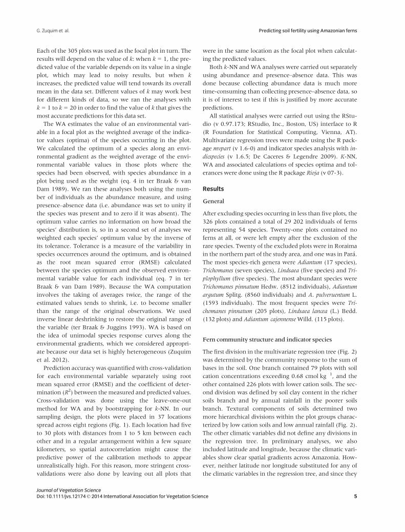
The first division in themultivariate regression tree (Fig. 2)

was determined by the community response to the sum of

bases in the soil. One branch contained 79 plots with soil

cation concentrations exceeding 0.68 cmol�kg�1, and the

other contained 226 plots with lower cation soils. The sec-

ond division was defined by soil clay content in the richer

soils branch and by annual rainfall in the poorer soils

branch. Textural components of soils determined two

more hierarchical divisions within the plot groups charac-

terized by low cation soils and low annual rainfall (Fig. 2).

The other climatic variables did not define any divisions in

the regression tree. In preliminary analyses, we also

included latitude and longitude, because the climatic vari-

ables show clear spatial gradients across Amazonia. How-

ever, neither latitude nor longitude substituted for any of

the climatic variables in the regression tree, and since they



are not direct environmental variables, they were left out

of the final analyses.

Most of the statistically significant indicator species were

associated with the branch containing the high cation sites

(Fig. 2). Nine out of 17 species of Adiantum were signifi-

cant indicators of this branch and only two Adiantum spe-

cies were significantly associated with the poorer soils

branch, although the genus as a whole was represented

over the entire gradient. Both Pteris species were also asso-

ciated with the richer soils branch. Almost all of the 18

richer soils indicator species were also significantly associ-

ated with the rich soils–high clay content branch in the

second level division.

Five out of seven Trichomanes species were indicators of

some secondary or tertiary division within the poorer soils

branch, and the very frequent T. pinnatum indicated poor

soils generally. Three out of five Lindsaea species were indi-

cators of the poorer soils branch and nonewas significantly

associated with the richer soils. The majority of poor soil

indicator species were associated with sites with relatively

high total annual rainfall (≥2163 mm). Only a few species

were indicators of habitats with both poor soils and low

rainfall.

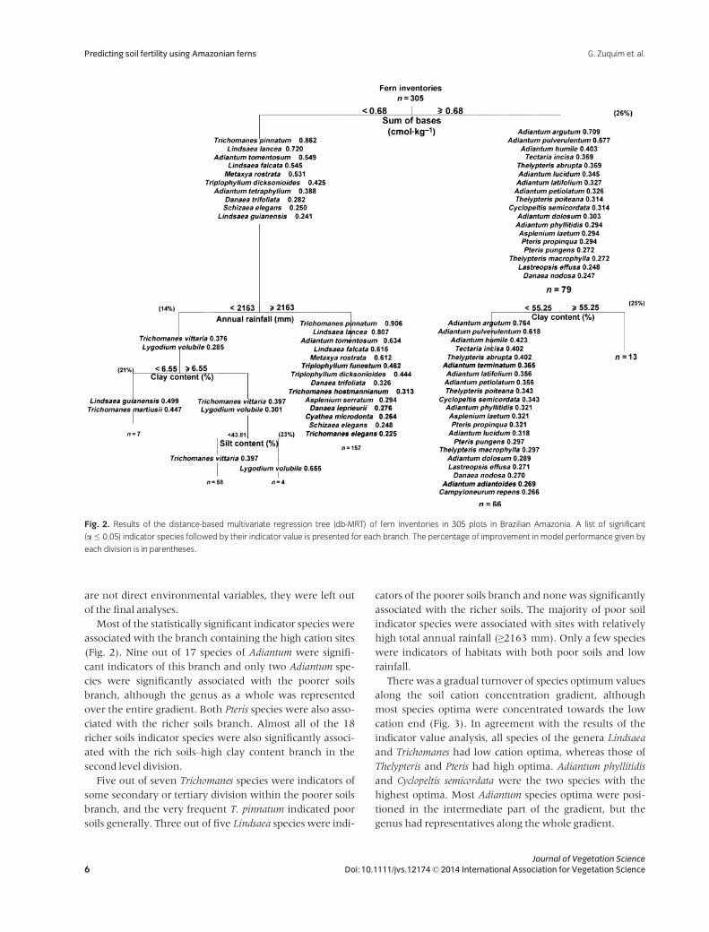
There was a gradual turnover of species optimum values

along the soil cation concentration gradient, although

most species optima were concentrated towards the low

cation end (Fig. 3). In agreement with the results of the

indicator value analysis, all species of the genera Lindsaea

and Trichomanes had low cation optima, whereas those of

Thelypteris and Pteris had high optima. Adiantum phyllitidis

and Cyclopeltis semicordata were the two species with the

highest optima. Most Adiantum species optima were posi-

tioned in the intermediate part of the gradient, but the

genus had representatives along the whole gradient.

Fig. 2. Results of the distance-based multivariate regression tree (db-MRT) of fern inventories in 305 plots in Brazilian Amazonia. A list of significant

(a ≤ 0.05) indicator species followed by their indicator value is presented for each branch. The percentage of improvement in model performance given by

each division is in parentheses.



Predicting environmental variables from fern

inventories

The edaphic variable that could be best predicted by fern

species composition was the sum of bases. All methods of

calibration produced R2 values that were between 0.64

and 0.75 when the focal plot was excluded in cross-valida-

tion. When all plots from the same locality as the focal plot

were excluded in leave-group-out cross-validation, R2 val-

ues decreased to between 0.46 and 0.64 (Table 2). There

was variation among the regions in the slope of the regres-

sion line between predicted and observed soil cation con-

centration, with the predictions for the Acre region

becoming especially inaccurate when leave-group-out

cross-validation was used (Fig. 4). The R2 values of the pre-

dictions for soil clay, sand and silt content were never

higher than 0.48 (Table 2). This is in accordance with the

regression tree results, which suggested that ferns respond

more strongly to soil cation concentrations than to soil tex-

tural properties.

The best results (smallest RMSEs) for predictions using

k-NN were achieved with between four and seven neigh-

bouring plots (k = 4 to k = 7). The differences in prediction

accuracy between k values in this range were generally

small, so for simplicity we report the results for k = 4 in all

cases. There were slight variations in prediction accuracy

among methods, but none of them was consistently better

than the others for all the edaphic variables. Weighted

averaging achieved lower RMSEs and higher R2 values

than k-NN when abundance data were used (Table 2), but

with presence–absence data, k-NN gave similar or higher

R2 values.

Weighting species by the inverse of their tolerance

improved the predictions in some cases but not univer-

sally. When leave-group-out cross-validation was used,

the differences in accuracy between weighted and non-

weighted estimations (R2 and RMSE) were small. In gen-

eral, the availability of abundance data did not improve

model performance. In fact, k-NN always performed better

with presence–absence data than with abundance data,

and evenWA did so inmost cases (Table 2).

Discussion

Earlier studies that have been carried out mostly in wes-

tern Amazonia have proposed that ferns and lycophytes

are good indicators of environmental conditions, especially

soil cation concentrations and particle size distributions

(Ruokolainen et al. 1997, 2007; Tuomisto et al. 2003a,c;

Higgins et al. 2011). Here we tested this proposal in central

Fig. 3. Estimated optima and tolerances of fern species along the sum of bases gradient across 305 plots in Brazilian Amazonia based on abundance data.

Values on the x-axis are presented on a logarithmic scale.



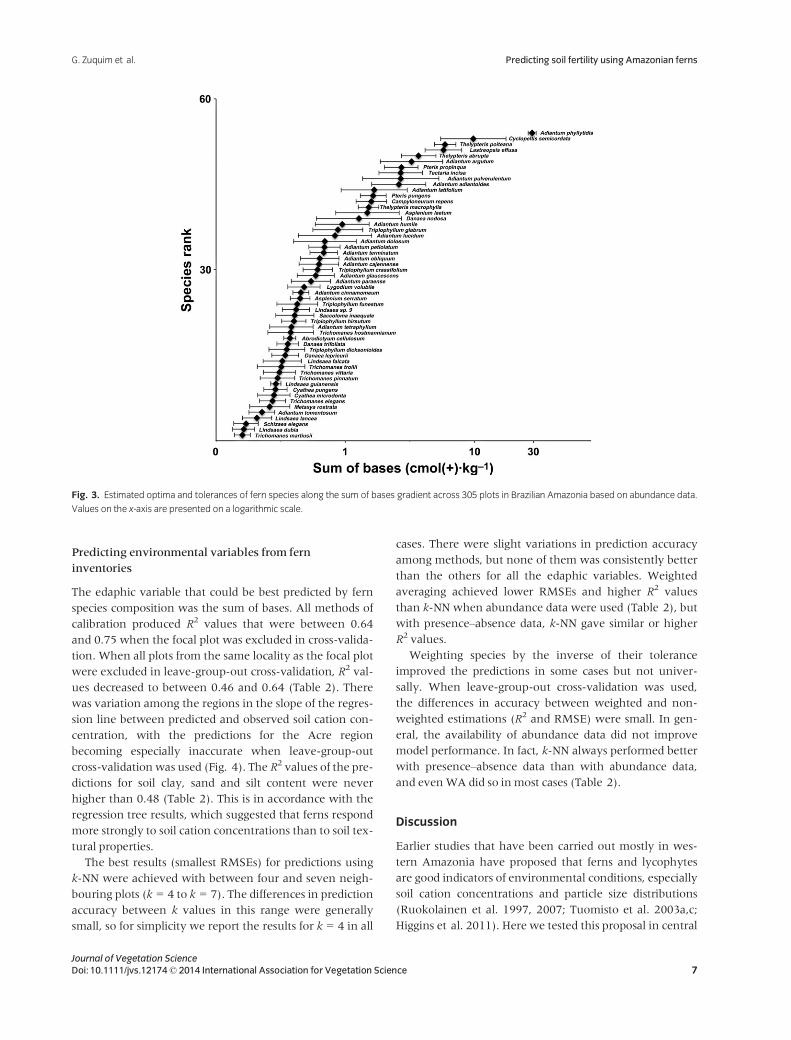
Table 2. Prediction accuracy given by the root mean squared error (RMSE) and coefficient of determination (R2) of the regressions between predicted and

observed edaphic properties in 305 plots in Brazilian Amazonia. The accuracy of the predictions for the k-nearest-neighbours (k-NN) method reported here

is based on k = 4 neighbours. The deshrinking method applied in weighted averaging (WA) was inverse deshrinking. Down-weighting in WA was done by

inversely weighting species optima by their tolerances along the environmental gradient when generating the predicted values. In k-NN, down-weighting

was done by inversely weighting the selected neighbouring plots by their floristic similarity to the focal. Cross-validation methods were bootstrap (k-NN)

and leave-one-out (WA) except when otherwise mentioned. ‘Crossval = lgo’ refers to leave-group-out cross-validation method and ‘Pres.-Abs.’ refers to

presence–absence input species data.

Species Log (sum of bases) Clay Silt Sand

Input data Downweighting RMSE R2 Crossval = lgo RMSE R2 RMSE R2 RMSE R2

RMSE R2

k-NN Abundance No 0.31 0.68 0.31 0.59 20.13 0.35 16.28 0.39 24.53 0.21

Similarity 0.33 0.64 0.32 0.59 20.10 0.35 16.82 0.35 25.15 0.14

Pres.-Abs. No 0.28 0.74 0.30 0.62 18.76 0.46 14.80 0.48 23.98 0.24

Similarity 0.28 0.75 0.31 0.64 19.54 0.41 15.65 0.43 24.24 0.19

WA Abundance No 0.29 0.65 0.33 0.55 18.67 0.30 14.53 0.37 22.15 0.18

Tolerance 0.27 0.70 0.36 0.46 18.10 0.34 14.00 0.41 21.79 0.20

Pres.-Abs. No 0.29 0.65 0.32 0.55 17.58 0.38 13.90 0.42 21.75 0.21

Tolerance 0.27 0.68 0.33 0.54 17.92 0.35 14.45 0.38 21.93 0.20

Fig. 4. Predicted vs observed sum of bases in 305 plots in Brazilian Amazonia. The grey line is the 1:1 line used in accuracy assessment, i.e. when

calculating the root mean squared errors (RMSEs) and R2 values. The solid black lines correponds to the regression line for all the predicted vs observed

values. Regression lines are also shown for each regional subset of the plots separately (broken lines) to illustrate the variation among regions. For

weighted averaging, the predicted values shown are those obtained after inverse deshrinking. Both axes are on a logarithmic scale.



Amazonia by making explicit predictions of soil properties

and climatic variables on the basis of information about

fern species composition.

Our results supported the conclusions of earlier studies.

The sum of bases emerged as the most important variable

in the regression tree, and was also the variable for which

the most accurate predictions could be obtained on the

basis of fern community composition. Soil textural and cli-

matic variation played secondary roles in the regression

tree, and soil texture was predicted less accurately than soil

base cation concentration. Soil texture is not a physiologi-

cally important edaphic factor, but it correlates with other

relevant environmental characteristics, such as nutrient

retention and water-holding capacity. Climate is also rel-

evant in structuring fern communities at broad scales

(Zuquim et al. 2012; Jones et al. 2013), but in the pres-

ent study its role was minor. This is in agreement with

the findings of Tuomisto & Poulsen (1996), who found

that even in a data set where annual rainfall varied

more than in ours, the main floristic gradient still

seemed to correspond to soil properties more than to

rainfall.

Predicting edaphic conditions from fern inventories

We found that sum of bases in the soil can be well pre-

dicted based on fern species composition. Our analyses

were carried out with log-transformed data, which means

that prediction errors related to large values of the variable

of interest are down-weighted. In other words, whether a

prediction is considered accurate or not depends more on

how large the error is in relation to the actual value of the

variable of interest, rather than on the absolute error

value. This is an appropriate model in the present context,

given that the final aim is to use the predicted soil values to

infer habitat characteristics and occurrence patterns for

such plant groups that have not been directly observed in

the field.

Another result that has practical implications is that pre-

diction accuracy for a particular environmental variable

was rather consistent among calibration methods. This

parallels the observations of Suominen et al. (2013), who

tested the k-NN and WA methods in western Amazonian

transects using the family Melastomataceae as a model

group. In a theoretical sense, both methods have their

strengths and weaknesses (Birks et al. 2010), but in practi-

cal applications both seem to perform equally well. As

could be expected, prediction accuracy appeared generally

higher when only the focal plot was left out of the training

set than when all the plots from the same site were left out

(R2 between 0.64 and 0.75 vs 0.46–0.64). Figure 4 shows

that the decrease in prediction accuracy was most notable

for the plots situated in Acre state, for which the predic-

tions fell dramatically below the observed values in the

leave-group-out cross-validation. This reflects the fact that

the plots in Acre had the highest observed cation concen-

trations in the entire data set, so when all of them were

excluded from the training set, no accurate analogue

remained for the Acre plots. As with other modelling

methods, attempts to extrapolate predictions of WA cali-

bration and k-NN estimation beyond the observed range of

the input variables can lead to seriously inaccurate results.

A third interesting result is that the prediction accuracies

for the edaphic variables were very similar whether species

presence–absence data or abundance data were used. Even

though we expected abundance data to provide better esti-

mates of species optima, and that this would lead to more

accurate predictions, this was not the case. One possible

reason is that the species abundances are so symmetrically

distributed along the relevant environmental gradients

that the optimum is in practice at the midpoint of the spe-

cies range, and can hence be identified equally well with

presence–absence and abundance data. Another possibility

is that species abundances depend on many different fac-

tors that are not necessarily linked to the factor being eval-

uated. For example, fertility may limit the range of species,

which is captured by presence–absence data, but may not

be the main driver of local abundances, which may be

controled by biotic interactions or more local factors such

as light. These unmeasured factors may cause a species to

be relatively abundant far away from its optimum for a

given variable, or not so abundant close to its optimum,

which then biases the estimate for that variable.

Earlier studies have obtained mixed results on whether

using abundance data increases or decreases the correla-

tions between species turnover and edaphic differences

(Tuomisto et al. 2003a; Ruokolainen et al. 2007). Our

results support the suggestion that at least when the

observed soil gradients are relatively long, presence–

absence data are adequate for many purposes (Tuomisto

et al. 2002, 2003a; Higgins & Ruokolainen 2004; Higgins

et al. 2011). This is good news, because collecting only

presence–absence data speeds up the fieldwork consider-

ably. Moreover, these results suggests that it is feasible to

tap edaphic information from non-quantitative species lists

and floras (e.g. Tuomisto & Poulsen 1996; Edwards 1998;

Costa et al. 1999, 2006; Freitas & Prado 2005; Costa & Pie-

trobom 2007; Maciel et al. 2007; Prado & Moran 2009;

Zuquim et al. 2009b), and perhaps even from herbarium

records through online databases such as GBIF. For exam-

ple, linking species lists with the species’ environmental

optima and tolerances enables inferences about site envi-

ronmental conditions. This opens up new and unexplored

possibilities for assessing representativeness of conserva-

tion area networks based on the use of readly available bio-

tic data as indicators of habitat types.



Species optima, tolerances and indicator values

It is noteworthy how well our results on species optima

agree with the suggestions made in earlier studies,

although the earlier data sets were much smaller, less

quantitative and represented a different geographical

region (e.g. Tuomisto & Poulsen 1996; Tuomisto et al.

1998, 2002, 2003b; C�ardenas et al. 2007). Such congru-

ence indicates that the inferences on the edaphic prefer-

ences of ferns have a good transferability across

geographical regions.

In our data set, the species optimum values were distrib-

uted along the entire gradient of soil cation concentration

(Fig. 3), but most of them were at the low end. This con-

trasts with the results of earlier studies, which have found

more fern species in high cation soils than in low cation

soils (Tuomisto & Poulsen 1996; Tuomisto et al. 2002,

2003b). The difference is likely due to biases in sampling.

Our data set contained many more plots with low cation

concentration than high cation concentration, and most of

the plots that in our data represent the high end of the gra-

dient were relatively cation-poor compared to the cation-

rich soils in the western Amazonian data. This probably

explains why most of the genera that in earlier studies

have been thought to indicate cation-rich soils (e.g. Diplazi-

um, Tectaria and Thelypteris) were absent or rare in our

data.

For those genera that werewell represented in both geo-

graphical areas, our results agreed with the earlier ones

from western Amazonia. The genus Adiantum was found

throughout the soil nutrient gradient, but most Adiantum

species occurred in intermediate to richer soils, in agree-

ment with the results of Tuomisto et al. (1998). They

observed that A. tomentosum and A. pulverulentum occur

at opposite ends of the soil cation gradient and never co-

occur, and this was the case also in our data.

Species differed in how accurate they seem to be as indi-

cators of environmental variables. For example, Trichom-

anes pinnatum had a high indicator value for cation-poor

soils in general, and some other species of the same genus

appeared as significant indicators for the finer clusters

within that group of sites. Although our sampling is rela-

tively extensive, it still covers only a small part of the envi-

ronmental variation within Amazonia. Therefore, the

optima and tolerances of species shown in Fig. 3 are still

preliminary, and should not be taken at face value. A

veiled gradient will push optimum values towards the

mean of the gradient for those species whose ranges

extend beyond the part of the gradient sampled, so the val-

ues we obtained for the species at the cation-rich end of

the gradient can be expected to be especially inaccurate.

However, the high congruence between our results and

those from western Amazonia suggest that the positions of

the species optima in relation to each other, and the

degrees of overlap in tolerance ranges, are probably rather

reliable.

The methods we used are based on general ecological

principles and can therefore be applied to any biogeo-

graphical area. The prerequisite is that the training data set

is suitable for the task at hand: it needs to cover the rele-

vant environmental gradients sufficiently well and to con-

tain an adequate number of species from the area of

interest. Our present data can be used as the training set

for other studies in central Amazonia, but studies focusing

on western or eastern Amazonia should complement the

training set locally. Failure to do so would compromise the

accuracy of the predictions, as illustrated with the rela-

tively low prediction accuracy for the Acre sites in the

leave-group-out cross-validation. At least one study in

Ecuadorian Amazonia (Sir�en et al. 2013) has produced a

map of estimated soil cation concentrations without hav-

ing had access to direct soil data from the area of interest.

Instead, they made fern inventories and used data from

existing inventories from other parts of NW Amazonia as

the training set to estimate soil cation concentrations

through calibration. Then they used satellite imagery to

generate extrapolated soil fertility maps. These kinds of

maps can be used to identify areas with different site condi-

tions, and thereafter to assess whether all the recognized

habitat variation is adequately represented in conservation

area networks.

Additional data with a more complete geographical cov-

erage will make it possible to select a limited number of

good indicator species that combine high environmental

specificity with sufficient frequency in suitable conditions

(Diekmann 2003). Indicator plants reflect environmental

conditions as integrated over extended time periods,

whereas soil samples give snapshot information of the

measured variables. Therefore, the species composition of

an indicator plant group can be expected to provide infor-

mation that is relevant for plants in general. The same

approach could also be tested in other relatively well

inventoried plant groups such as palms (Svenning 1999;

Vormisto et al. 2000; Costa et al. 2009), trees (Pitman

et al. 2001; Castilho et al. 2006; Stropp et al. 2009) and

gingers (Figueiredo et al. 2013). Our results demonstrate

that the species and environmental data sets already avail-

able in the Amazon region are a good starting point

towards better tools andmaps for conservation planning.

Acknowledgements

We thank several field assistants thatmade this work possi-

ble. ICMBIO provided permits and infrastructure facilities.

Financial support for fieldwork was provided by Biological

Dynamics of Forest Fragments (BDFFP), MCT/CNPq/PPG7



no. 48/2005 (led byWilliam E. Magnusson), Brazilian Pro-

gram of Biodiversity Research – PPBio, CNPq/FAPEAM/

PRONEX project no. 673/2010 (led byWilliam E. Magnus-

son, INPA), FINEP/Projeto Integrado MCT-EMBRAPA (led

by Ana L. K. M. Albernaz), Hidroveg Project – FAPEAM/

FAPESP no. 1428/2010 (led by Fl�avia R. C. Costa and Ja-

vier Tomasella). Gabriela Zuquim was supported by CNPq,

CAPES and Academy of Finland (research grant to Hanna

Tuomisto). We thank Lassi Suominen for helpful com-

ments on the manuscript. Many people are acknowledged

for their efforts to make data and analytical tools freely

available. This is publication number 627 ST of the BDFFP

technical series.

References

Birks, H.J.B., Line, J.M., Juggins, S., Stevenson, A.C., & ter Bra-

ak, C.J.F. 1990. Diatoms and pH reconstruction. Philosophical

Transactions of the Royal Society of London Series B, Biological Sci-

ences 327: 263–278.

Birks, H.J.B., Heiri, O., Sepp€a, H., & Bjune, A.E. 2010. Strengths

and weaknesses of quantitative climate reconstructions

based on late-quaternary biological proxies. The Open Ecology

Journal 3: 68–110.

C�ardenas, G.G., Halme, K.J., & Tuomisto, H. 2007. Riqueza y dis-

tribuci�on ecol�ogica de especies de pteridofitas en la zona del

r�ıo Yavar�ı-Mir�ın, Amazon�ıa Peruana. Biotropica 39: 637–646.

Castilho, C.V., Magnusson, W.E., Ara�ujo, R.N.O., Luiz~ao,

R.C.C., Luiz~ao, F.J., Lima, A.P., & Higuchi, N. 2006. Varia-

tion in aboveground tree live biomass in a central Amazo-

nian Forest: Effects of soil and topography. Forest Ecology and

Management 234: 85–96.

Chauvel, A., Lucas, Y., & Boulet, R. 1987. On the genesis of the

soil mantle of the region of Manaus, Central Amazonia, Bra-

zil. Experientia 43: 234–240.

Costa, J.M. & Pietrobom, M.R. 2007. Pterid�ofitas (Lycophyta e

Monilophyta) da Ilha de Mosqueiro, munic�ıpio de Bel�em,

estado do Par�a, Brasil. Boletim do Museu Paraense Em�ılio Goeldi.

Ciencias Naturais 2: 45–56.

Costa, M.A.S., Prado, J., Windisch, P.G., Freitas, C.A.A., & La-

biak, P. 1999. Pteridophyta. In: Ribeiro, J.E.L.S., Hopkins,

M.J.G., Vicentini, A., Sothers, C.A., Costa, M.A.S., Brito,

J.M., Souza, M.A., Martins, L.H., Lohmann, L.G., (. . .) &

Proc�opio, L.C. (eds.) Flora da Reserva Ducke – Guia de identi-

ficac�~ao das plantas vasculares de uma floresta de terra firme na

Amazonia Central, pp. 97–117. Editora INPA,Manaus, BR.

Costa, F.R.C., Magnusson, W.E., & Luiz~ao, R.C. 2005. Mesoscale

distribution patterns of Amazonian understorey herbs in

relation to topography, soil andwatersheds. Journal of Ecology

93: 863–878.

Costa, J.M., Souza, M.G.C., & Pietrobom, M.R. 2006. Levanta-

mento flor�ıstico das Pterid�ofitas (Lycophyta e Monilophyta)

do Parque Ambiental de Bel�em (Bel�em, Par�a, Brasil). Revista

de Biologia Neotropical 3: 4–12.

Costa, F.R., Guillaumet, J.-L., Lima, A.P., & Pereira, O.S. 2009.

Gradients within gradients: The mesoscale distribution pat-

terns of palms in a central Amazonian forest. Journal of Vege-

tation Science 20: 69–78.

De Caceres, M. & Legendre, P. 2009. Associations between spe-

cies and groups of sites: indices and statistical inference. Ecol-

ogy 90: 3566–3574.

De’ath, G. 1999. Extended dissimilarity: a method of robust esti-

mation of ecological distances from high beta diversity data.

Plant Ecology 144: 191–199.

De’ath, G. 2002. Multivariate regression trees: a new technique

for modeling species–environment relationships. Ecology 83:

1105–1117.

Diekmann, M. 2003. Species indicator values as an important

tool in applied plant ecology – a review. Basic and Applied

Ecology 4: 493–506.

Dijkshoorn, J.A., Huting, J.R.M., & Tempel, P. 2005.Update of the

1:5 million Soil and Terrain Database for Latin America and

the Caribbean (SOTERLAC; version 2.0). Available at http://

www.isric.org/sites/default/files/ISRIC_Report_2005_01.pdf

Accessed 27 February 2014.

Dufrene, M. & Legendre, P. 1997. Species assemblages and indi-

cator species: the need for a flexible asymmetrical approach.

Ecological Monographs 67: 345–366.

Edwards, P.J. 1998. The pteridophytes of the Ilha de Marac�a. In:

Milliken, W. & Ratter, J.A. (eds.) Marac�a: the biodiversity and

environment of an Amazonian rainforest. John Wiley & Sons,

Chichester, UK.

Emilio, T., Nelson, B.W., Schietti, J., Desmouli�ere, S.J.-M.,

Esp�ırito Santo, H.M.V., & Costa, F.R.C. 2010. Assessing the

relationship between forest types and canopy tree beta diver-

sity in Amazonia. Ecography 33: 738–747.

Figueiredo, F.O.G., Costa, F.R.C., Nelson, B.W., & Pimentel, T.P.

2013. Validating forest types based on geological and land-

form features in central Amazonia. Journal of Vegetation

Science 25: 198–212.

Freitas, C.A.A. & Prado, J. 2005. Lista anotada das pterid�ofitas de

florestas inund�aveis do alto Rio Negro, Munic�ıpio de Santa

Isabel do Rio Negro, AM, Brasil. Acta Botanica Brasilica 19:

399–406.

Higgins, M.A. & Ruokolainen, K. 2004. Rapid tropical forest

inventory: a comparison of techniques based on inventory

data from western Amazonia. Conservation Biology 18: 799–

811.

Higgins, M.A., Ruokolainen, K., Tuomisto, H., Llerena, N., Card-

enas, G., Phillips, O.L., Vasquez, R., & R€as€anen, M. 2011.

Geological control of floristic composition in Amazonian for-

ests. Journal of Biogeography 38: 2136–2149.

Hijmans, R.J., Cameron, S.E., Parra, J.L., Jones, P.G., & Jarvis, A.

2005. Very high resolution interpolated climate surfaces for

global land areas. International Journal of Climatology 25:

1965–1978.

Hijmans, R.J., Guarino, L., & Mathur, P. 2012. DIVA-GIS Version

7.5. Manual. Available at http://www.diva-gis.org/docs/

DIVA-GIS_manual_7.pdf Accessed 14March 2014.



Howard, P.C., Viskanic, P., Davenport, T.R.B., Kigenyi, F.W.,

Baltzer, M., Dickinson, C.J., Lwanga, J.S., Matthews, R.A., &

Balmford, A. 1998. Complementarity and the use of indica-

tor groups for reserve selection in Uganda. Nature 394: 472–

475.

IBGE – Instituto Brasileiro de Geografia e Estat�ıstica. 2004. Mapa

de Vegetac�~ao do Brasil. 3rd ed. Available at ftp://ftp.ibge.

gov.br/Cartas_e_Mapas/Mapas_Murais/ Accessed 14 March

2014.

Jones, M.M., Tuomisto, H., Clark, D.B., & Olivas, P. 2006. Effects

of mesoscale environmental heterogeneity and dispersal lim-

itation on floristic variation in rain forest ferns. Journal of

Ecology 94: 181–195.

Jones, M.M., Ferrier, S., Condit, R., Manion, G., Aguilar, S., &

P�erez, R. 2013. Strong congruence in tree and fern commu-

nity turnover in response to soils and climate in central Pan-

ama. Journal of Ecology 101: 506–516.

Kinupp, V.F. & Magnusson, W.E. 2005. Spatial patterns in the

understorey shrub genus Psychotria in central Amazonia:

effects of distance and topography. Journal of Tropical Ecology

21: 363–374.

Legendre, P. & Legendre, L. 1998. Numerical Ecology. 2nd ed.

Elsevier, Amsterdam, NL.

Maciel, S., Souza, M.G.C., & Pietrobom, M.R. 2007. Lic�ofitas e

monil�ofitas do Bosque Rodrigues Alves Jardim Botanico da

Amazonia, munic�ıpio de Bel�em, estado do Par�a, Brasil. Bole-

tim do Museu Paraense Em�ılio Goeldi. Ciencias Naturais 2: 69–83.

Magnusson, W.E., Lima, A.P., Luiz~ao, R.C.C., Luiz~ao, F., Costa,

F.R.C., Castilho, C.V., & Kinupp, V.P. 2005. RAPELD: a mod-

ification of the Gentry method for biodiversity surveys in

long-term ecological research sites. Biota Neotropica 5(2).

Available at http://www.biotaneotropica.org.br/v5n2/pt/

download?point-of-view+bn01005022005+abstract Accessed

27 February 2014.

Margules, C.R., Pressey, R.L., & Williams, P.H. 2002. Represent-

ing biodiversity: data and procedures for identifying priority

areas for conservation. Journal of Biosciences 27: 309–326.

McGeoch, M.A. 1998. The selection, testing and application of

terrestrial insects as bioindicators. Biological Reviews 73: 181–

201.

Mertens, J. 2004. The characterization of selected physical and chemi-

cal soil properties of the surface soil layer in the ‘Reserva Ducke’,

Manaus, Brazil, with emphasis on their spatial distribution. Bach-

elor thesis, Humboldt University, Berlin, DE.

Noss, R.F. 1990. Indicators for monitoring biodiversity: a hierar-

chical approach. Conservation Biology 4: 355–364.

Phillips, O.L., Vargas, P.N., Monteagudo, A.L., Cruz, A.P., Zans,

M.-E.C., S�anchez,W.G., Yli-Halla, M., & Rose, S. 2003. Habi-

tat association among Amazonian tree species: a landscape-

scale approach. Journal of Ecology 91: 757–775.

Pitman, N.C.A., Terborgh, J.W., Miles, R., Silman, P.N.V., Neill,

D.A., Cer�on, C.E., Palacios,W.A., & Aulestia, M. 2001. Dom-

inance and distribution of tree species in upper Amazonian

terra firme forests. Ecology 83: 2101–2117.

Prado, J. & Moran, R.C. 2009. Checklist of the ferns and lyco-

phytes of Acre state, Brazil. Fern Gazette 18: 230–263.

Quesada, C.A., Lloyd, J., Anderson, L.O., Fyllas, N.M., Schwarz,

M., & Czimczik, C.I. 2011. Soils of Amazonia with particular

reference to the RAINFOR sites. Biogeosciences 8: 1415–1440.

RADAMBRASIL 1978. Projeto RADAMBRASIL. Vol. (1:34).

Geologia geomorfologia, pedologia, vegetac�~ao e uso poten-

cial da terra. Departamento Nacional de Produc�~ao Mineral.

Rio de Janeiro.

Ruokolainen, K., Linna, A., & Tuomisto, H. 1997. Use of Melas-

tomataceae and pteridophytes for revealing phytogeographi-

cal patterns in Amazonian rain forests. Journal of Tropical

Ecology 13: 243–256.

Ruokolainen, K., Tuomisto, H., Mac�ıa, M.J., Higgins, M.A.,

& Yli-Halla, M. 2007. Are floristic and edaphic patterns

in Amazonian rain forests congruent for trees, pterido-

phytes and Melastomataceae? Journal of Tropical Ecology

23: 13–25.

Salovaara, K.J., C�ardenas, G.G., & Tuomisto, H. 2004. Forest

classification in an Amazonian rainforest landscape using

pteridophytes as indicator species. Ecography 27: 689–700.

Schulman, L., Toivonen, T., & Ruokolainen, K. 2007a. Analysing

botanical collecting effort in Amazonia and correcting for it

in species range estimation. Journal of Biogeography 34:

1388–1399.

Schulman, L., Ruokolainen, K., Junikka, L., S€a€aksj€arvi, I.E.,

Salo, M., Juvonen, S., Salo, J., & Higgins, M. 2007b. Amazo-

nian biodiversity and protected areas: do they meet? Biodi-

versity and Conservation 16: 3011–3051.

Sir�en, A., Tuomisto, H., & Navarrete, H. 2013. Mapping environ-

mental variation in lowland Amazonian rainforests using

remote sensing and floristic data. International Journal of

Remote Sensing 34: 1561–1575.

Stropp, J., ter Steege, H., Malhi, Y., ATDN, & RAINFOR. 2009.

Disentangling regional and local tree diversity in the Ama-

zon. Ecography 32: 46–54.

Suominen, L., Ruokolainen, K., Tuomisto, H., Llerena, N., & Hig-

gins, M.A. 2013. Predicting soil properties from floristic com-

position in western Amazonian rainforests: performance of

k-nearest neighbour estimation andweighted averaging cali-

bration. Journal of Applied Ecology 50: 1441–1449.

Svenning, J.-C. 1999. Microhabitat specialization in a species-

rich palm community in Amazonian Ecuador. Journal of Ecol-

ogy. 87: 55–65.

ter Braak, C.J.F. & Juggins, S. 1993. Weighted averaging partial

least squares regression (WA-PLS): an improved method for

reconstructing environmental variables from species assem-

blages.Hydrobiologia 269/270: 485–502.

ter Braak, C.J.F. & van Dam, H. 1989. Inferring pH from diatoms:

a comparison of old and new calibration methods. Hydrobio-

logia 178: 209–223.

Tuomisto, H. 2006. Edaphic niche differentiation among Polybot-

rya ferns in Western Amazonia: implications for coexistence

and speciation. Ecography 29: 273–284.



Tuomisto, H. & Poulsen, A.D. 1996. Influence of edaphic special-

ization on the distribution of pteridophytes in neotropical

forests. Journal of Biogeography 23: 283–293.

Tuomisto, H., Poulsen, A.D., &Moran, R.C. 1998. Edaphic distri-

bution of some species of the fern genus Adiantum in Wes-

tern Amazonia. Biotropica 30: 392–399.

Tuomisto, H., Ruokolainen, K., Poulsen, A.D., Moran, R.C.,

Quintana, C., Ca~nas, G., & Celi, J. 2002. Distribution and

diversity of pteridophytes and Melastomataceae along

edaphic gradients in Yasun�ı national park, Ecuadorian

Amazonia. Biotropica 34: 516–533.

Tuomisto, H., Ruokolainen, K., & Yli-Halla, M. 2003a. Dispersal,

environmental, and floristic variation of Western Amazo-

nian forests. Science 299: 241–244.

Tuomisto, H., Ruokolainen, K., Aguilar, M., & Sarmiento, A.

2003b. Floristic patterns along a 43-km long transect in an

Amazonian rain forest. Journal of Ecology 91: 743–756.

Tuomisto, H., Poulsen, A.D., Ruokolainen, K., Moran, R.C.,

Quintana, C., Celi, J., & Ca~nas, G. 2003c. Linking floristic

patterns with soil heterogeneity and satellite imagery

in Ecuadorian Amazonia. Ecological Applications 13: 352–

371.

Tuomisto, H., Ruokolainen, L., & Ruokolainen, K. 2012.

Modelling niche and neutral dynamics: on the ecological

interpretation of variation partitioning results. Ecography 35:

961–971.

Vormisto, J., Phillips, O., Ruokolainen, K., Tuomisto, H., &

V�asquez, R. 2000. A comparison of fine-scale distribution

patterns of four plant groups in an Amazonian rainforest.

Ecography 23: 349–359.

Zuquim, G., Costa, F.R.C., Prado, J., & Braga-Neto, R. 2009a.

Distribution of pteridophyte communities along environ-

mental gradients in Central Amazonia, Brazil. Biodiversity

and Conservation 18: 151–166.

Zuquim, G., Prado, J., & Costa, F.R.C. 2009b. An annotated

checklist of ferns and lycophytes from the Biological Reserve

of Uatum~a, an area with patches of rich soils in central

Amazonia, Brazil. Fern Gazette 18: 286–306.

Zuquim, G., Tuomisto, H., Costa, F.R.C., Prado, J., Magnusson,

W.E., Pimentel, T., Braga-Neto, R., & Figueiredo, F.O.G.

2012. Broad Scale distribution of ferns and lycophytes along

environmental gradients in Central and Northern Amazonia,

Brazil. Biotropica 44: 752–762.

Supporting Information

Additional supporting information may be found in the

online version of this article:

Appendix S1.Detailed study locations description.



JournalofVegetationScience && (2014 ... · JournalofVegetationScience&& (2014)...

Documents

Transcript of JournalofVegetationScience && (2014 ... · JournalofVegetationScience&& (2014)...