Journal of Econometrics 191 (2016) 384–397

Contents lists available at ScienceDirect

Journal of Econometrics

journal homepage: www.elsevier.com/locate/jeconom

Improving GDP measurement: A measurement-error perspectiveS. Borağan Aruoba a,∗, Francis X. Diebold b, Jeremy Nalewaik c, Frank Schorfheide b,Dongho Song d

a University of Maryland, United Statesb University of Pennsylvania, United Statesc Federal Reserve Board, United Statesd Boston College, United States

a r t i c l e i n f o

Article history:Available online 7 December 2015

JEL classification:E01E32

Keywords:IncomeOutputExpenditureBusiness cycleExpansionContractionRecessionTurning pointState-space modelDynamic factor modelForecast combination

a b s t r a c t

We provide a newmeasure of historical U.S. GDP growth, obtained by applying optimal signal-extractiontechniques to the noisy expenditure-side and income-side GDP estimates. The quarter-by-quarter valuesof our newmeasure often differ noticeably from those of the traditional measures. Its dynamic propertiesdiffer as well, indicating that the persistence of aggregate output dynamics is stronger than previouslythought.

© 2015 Elsevier B.V. All rights reserved.

1. Introduction

Aggregate real output is surely the most fundamental and im-portant concept in macroeconomic theory. Surprisingly, however,significant uncertainty still surrounds its historical measurement.In the U.S., in particular, two often-divergent GDP estimates ex-ist, a widely-used expenditure-side version, GDPE , and a muchless widely-used income-side version, GDPI .1 Nalewaik (2010)and Fixler and Nalewaik (2009) make clear that, at the very least,GDPI deserves serious attention and may even have properties incertain respects superior to those of GDPE .2 That is, if forced tochoose between GDPE and GDPI , a surprisingly strong case exists

∗ Corresponding author.E-mail addresses: aruoba@econ.umd.edu (S.B. Aruoba),

fdiebold@sas.upenn.edu (F.X. Diebold), jeremy.j.nalewaik@frb.gov (J. Nalewaik),schorf@ssc.upenn.edu (F. Schorfheide), dongho.song@bc.edu (D. Song).1 Indeed we will focus on the U.S. because it is a key egregious example of

unreconciled GDPE and GDPI estimates.2 For additional informative background on GDPE , GDPI , the statistical discrep-

ancy, and the national accounts more generally, see BEA (2006), McCulla and Smith(2007), Landefeld et al. (2008), and Rassier (2012).

http://dx.doi.org/10.1016/j.jeconom.2015.12.0090304-4076/© 2015 Elsevier B.V. All rights reserved.

for GDPI . But of course one is not forced to choose between GDPEand GDPI , and a GDP estimate based on both GDPE and GDPI maybe superior to either one alone. In this paper we propose and im-plement a framework for obtaining such a blended estimate.

Our work is related to, and complements, (Aruoba et al., 2012).There we took a forecast-error perspective, whereas here wetake a measurement-error perspective.3 In particular, we workwith a dynamic factor model in the tradition of Geweke (1977)and Sargent and Sims (1977), as used and extended byWatson andEngle (1983), Edwards and Howrey (1991), Harding and Scutella(1996), Jacobs and van Norden (2011), Kishor and Koenig (2012),and Fleischman and Roberts (2011), among others.4 That is, weview ‘‘true GDP ’’ as a latent variable on which we have several

3 Hence the pair of papers roughly parallels the well-known literature on‘‘forecast error’’ and ‘‘measurement error’’ properties of data revisions; see forexample Mankiw et al. (1984), Mankiw and Shapiro (1986), Faust et al. (2005),and Aruoba (2008).4 See also Smith et al. (1998), who take a different but related approach, and

the independent work of Greenaway-McGrevy (2011), who takes a closely-relatedapproach but unfortunately estimates a model that we show to be unidentified inSection 2.3.

S.B. Aruoba et al. / Journal of Econometrics 191 (2016) 384–397 385

indicators, the twomost obvious beingGDPE andGDPI , andwe thenextract true GDP using optimal filtering techniques.

The measurement-error approach is time honored, intrinsi-cally compelling, and very different from the forecast-combinationperspective of Aruoba et al. (2012), for several reasons.5 First, itenables extraction of latent true GDP using a model with parame-ters estimatedwith exact likelihood or Bayesian methods, whereasthe forecast-combination approach forces one to use calibrated pa-rameters. Second, it delivers not only point extractions of latenttrue GDP but also interval extractions, enabling us to assess the as-sociated uncertainty. Third, the state-space framework in whichthe measurement-error models are embedded facilitates explo-ration of the relationship between GDP measurement errors andthe economic environment, such as stage of the business cycle,which is of special interest.

We proceed as follows. In Section 2 we consider severalmeasurement-error models and assess their identification status,which turns out to be challenging and interesting in the most real-istic and hence compelling case. In Section 3 we discuss the data,estimation framework and estimation results. In Section 4 we ex-plore the properties of our new GDP series. Finally, we concludewith both a summary and a caveat in Section 5, where the caveatrefers to the potential limitations ofGDPI (relative toGDPE) for real-time analysis.

2. Five measurement-error models of GDP

We use dynamic-factor measurement-error models, whichembed the idea that both GDPE and GDPI are noisy measuresof latent true GDP . We work throughout with growth rates ofGDPE , GDPI and GDP (hence, for example, GDPE denotes a growthrate).6 We assume throughout that true GDP growth evolves withsimple AR(1) dynamics, and we entertain several measurementstructures, to which we now turn.

2.1. (Identified) 2-equation model: Σ diagonal

We begin with the simplest 2-equation model; the measure-ment errors are orthogonal to each other and to transition shocksat all leads and lags.7 Themodel has a natural state-space structure,and we writeGDPEtGDPIt

=

11

GDPt +

ϵEtϵIt

(1)

GDPt = µ(1 − ρ) + ρGDPt−1 + ϵGt ,

where GDPEt and GDPIt are expenditure- and income-side es-timates, respectively, GDPt is latent true GDP , and all shocksare Gaussian and uncorrelated at all leads and lags. That is,(ϵGt , ϵEt , ϵIt)

′∼ iid N(0, Σ), where

Σ =

σ 2GG 0 00 σ 2

EE 00 0 σ 2

II

. (2)

The Kalman smootherwill deliver optimal extractions ofGDPt con-ditional upon observed expenditure- and income-side measure-ments.Wewill refer tomeasures ofGDP obtained thisway asGDPMthroughout the paper.Moreover, themodel can be easily extended,and some of its restrictive assumptions relaxed, with no funda-mental change. We now proceed to do so.

5 On the time-honored aspect, see, for example, Gartaganis and Goldberger(1955).6 We will elaborate on the reasons for this choice later in Section 3.7 Here and throughout, when we say ‘‘N-equation’’ state-space model, we mean

that the measurement equation is an N-variable system.

2.2. (Identified) 2-equation model: Σ block-diagonal

The first extension is to allow for correlated measurementerrors. This is surely important, as there is roughly a 25% overlap inthe counts embedded in GDPE and GDPI , and moreover, the samedeflator is used for conversion from nominal to real magnitudes.8We writeGDPEtGDPIt

=

11

GDPt +

ϵEtϵIt

(3)

GDPt = µ(1 − ρ) + ρGDPt−1 + ϵGt ,

where now ϵEt and ϵIt may be correlated contemporaneously butare uncorrelated at all other leads and lags, and all other definitionsand assumptions are as before; in particular, ϵGt and (ϵEt , ϵIt)

′

are uncorrelated at all leads and lags. That is, (ϵGt , ϵEt , ϵIt)′

∼

iid N(0, Σ), where

Σ =

σ 2GG 0 00 σ 2

EE σ 2EI

0 σ 2IE σ 2

II

. (4)

Nothing is changed, and the Kalman filter retains its optimalityproperties.

2.3. (Unidentified) 2-equation model, Σ unrestricted

The second key extension is motivated by Fixler and Nalewaik(2009) and Nalewaik (2010), who document cyclicality in the sta-tistical discrepancy (GDPE − GDPI ), which implies failure of theassumption that (ϵEt , ϵIt)

′ and ϵGt are uncorrelated at all leadsand lags. Of particular concern is contemporaneous correlation be-tween ϵGt and (ϵEt , ϵIt)

′. Hence we allow the measurement errors(ϵEt , ϵIt)

′ to be correlated with GDPt , or more precisely, correlatedwith GDPt innovations, ϵGt . We writeGDPEtGDPIt

=

11

GDPt +

ϵEtϵIt

(5)

GDPt = µ(1 − ρ) + ρGDPt−1 + ϵGt ,

where (ϵGt , ϵEt , ϵIt)′∼ iid N(0, Σ), with

Σ =

σ 2GG σ 2

GE σ 2GI

σ 2EG σ 2

EE σ 2EI

σ 2IG σ 2

IE σ 2II

. (6)

In this environment the standard Kalman filter is rendered sub-optimal for extracting GDP , due to correlation between ϵGt and(ϵEt , ϵIt), but appropriately-modified optimal filters are available.

Of course in what follows we will be concerned with esti-mating our measurement-equation models, so we will be con-cerned with identification. The diagonal-Σ model (1)–(2) and theblock-diagonal-Σ model (3)–(4) are identified. Identification ofless-restricted dynamic factor models, however, is a very delicatematter. In particular, it is not obvious that the unrestricted-Σmodel (5)–(6) is identified. Indeed it is not, as we prove in Ap-pendix A. Hence we now proceed to determine minimal restric-tions that achieve identification.

2.4. (Identified) 2-equation model: Σ restricted

The identification problem with the general model (5)–(6)stems from the fact that we can make true GDP more volatile (in-

8 See Aruoba et al. (2012) for more. Many of the areas of overlap are particularlypoorly measured, such as imputed financial services, housing services, andgovernment output.

386 S.B. Aruoba et al. / Journal of Econometrics 191 (2016) 384–397

crease σ 2GG) and make the measurement errors more volatile (in-

crease σ 2EE and σ 2

II ), but reduce the covariance between the funda-mental shocks and the measurement errors (reduce σ 2

EG and σ 2IG),

without changing the distribution of observables.

2.4.1. Restricting the original parameterizationWe can achieve identification by slightly restricting parameter-

ization (5)–(6). In particular, as we show in Appendix A, the unre-stricted system (5)–(6) is unidentified because the Σ matrix hassix free parameters with only five moment conditions to deter-mine them. Hence we can achieve identification by restricting anysingle element of Σ . Imposing any such restriction would seemchallenging, however, as we have no strong prior views directlyon any single element of Σ . Fortunately, however, a simple re-parameterization exists about which we have a more natural priorview, to which we now turn.

2.4.2. A useful re-parameterizationLet

ζ =

11−ρ2 σ

2GG

11−ρ2 σ

2GG + 2σ 2

GE + σ 2EE

, (7)

the variance of latent true GDP relative to the variance ofexpenditure-side measured GDPE . Then, rather than fixing anelement of Σ to achieve identification, we can fix ζ , about whichwe have a more natural prior view. In particular, at first pass wemight take σ 2

GE ≈ 0, in which case 0 < ζ < 1. Or, put differently,ζ > 1would require a very negative σ 2

GE , which seems unlikely. Alltold, we view a ζ value less than, but close to, 1.0 as most natural.We take ζ = 0.80 as our benchmark in the empirical work thatfollows, although we explore a wide range of ζ values both belowand above 1.0.

2.5. (Identified) 3-equation model: Σ unrestricted

Thus far we showed how to achieve identification by fixinga parameter, ζ , and we noted that our prior is centered aroundζ = 0.80. It is also of interest to know whether we can get somecomplementary data-based guidance on choice of ζ . The answerturns out to be yes, by adding a third measurement equation witha certain structure.

Suppose, in particular, that we have an additional observablevariable Ut that loads on true GDPt with measurement errororthogonal to those of GDPI and GDPE . In particular, consider the3-equation modelGDPEtGDPItUt

=

00κ

+

11λ

GDPt +

ϵEtϵItϵUt

(8)

GDPt = µ(1 − ρ) + ρGDPt−1 + ϵGt ,

where (ϵGt , ϵEt , ϵIt , ϵUt)′∼ iid N(0, Ω), with

Ω =

σ 2GG σ 2

GE σ 2GI σ 2

GU

σ 2EG σ 2

EE σ 2EI 0

σ 2IG σ 2

IE σ 2II 0

σ 2UG 0 0 σ 2

UU

. (9)

Note that the upper-left 3 × 3 block of Ω is just Σ , whichis now unrestricted. Nevertheless, as we prove in Appendix B,the 3-equation model (8)–(9) is identified. Of course some ofthe remaining elements of the overall 4 × 4 covariance matrixΩ are restricted, which is how we achieve identification in the3-equation model, but the economically interesting sub-matrix,

which the 3-equation model leaves completely unrestricted,is Σ .

Depending on the application, of course, it is not obvious thatan identifying variable Ut with measurement errors orthogonalto those of GDPE and GDPI (i.e., with stochastic properties thatsatisfy (9)), is available. Hence it is not obvious that estimation ofthe 3-equation model (8)–(9) is feasible in practice, despite themodel’s appeal in principle. Indeed, much of the data collectedfrom business surveys is used in the BEA’s estimates, invalidatinguse of that data as Ut since any measurement error in that dataappears directly in either GDPE or GDPI , producing correlationacross the measurement errors. Moreover, variables drawn frombusiness surveys similar to those used to produce GDPE and GDPI ,even if they are not used directly in the estimation of GDPE andGDPI , might still be invalid identifying variables if the surveymethodology itself produces similar measurement errors.9

Fortunately, however, some important macroeconomic data iscollected not from surveys of businesses, but from samples ofhouseholds. A sample of data drawn from a universe of householdsseems likely to have measurement errors that are different thanthose contaminating a data sample drawn from a universe ofbusinesses, especially when the ‘‘universes’’ of businesses andhouseholds are not complete census counts, as is the case here.For example, the universe of business surveys is derived from taxrecords, so businesses not paying taxes will not appear on thatlist, but individuals working at that business may appear in theuniverse of households.

Importantly, very little data collected from household surveysare used to construct GDPE and GDPI , so a Ut variable computedfrom a household survey seems most likely to meet ouridentification conditions. The change in the unemployment rate isa natural choice (hence our notational choiceUt ).Ut arguably loadson trueGDP with ameasurement error orthogonal to those ofGDPEand GDPI , because the Ut data is being produced independently(by the BLS rather than BEA) from different types of surveys. Inaddition, virtually all of the GDPE and GDPI data are estimated innominal dollars and then converted to real dollars using a pricedeflator, whereas Ut is estimated directly with no deflation.

All told, we view ‘‘3-equation identification’’ as a useful com-plement to the ‘‘ζ -identification’’ discussed earlier in Section 2.4.All identifications involve assumptions. ζ -identification involvesintrospection about likely values of ζ , given its structure andcomponents, and that introspection is of course subject to er-ror. 3-equation identification involves introspection about variousmeasurement-error correlations involving the newly-introducedthird variable, which is of course also subject to error. Indeed thetwo approaches to identification are usefully used in tandem, andcompared.

One can even view the 3-equation approach as a device forimplicitly selecting ζ . In particular, we can find the ζ implied bythe 3-equation model estimate, that is, find the ζ that minimizesthe divergence between Σζ and Σ3, in an obvious notation.10 Forexample, using the Frobeniusmatrix-norm tomeasure divergence,we obtain an optimum of ζ ∗

= 0.82. The minimum is sharpand unique. The implied ζ ∗ of 0.82 is of course quite close to thedirectly-assessed value of 0.80 at which we arrived earlier, whichlends additional credibility to the earlier assessment. See (online)Appendix C.2.1 for details.

9 For example, if the business surveys used to produce GDPE and GDPI tendto oversample large firms, variables drawn from a business survey that alsooversamples large firms may have measurement errors that are correlated withthose in GDPE and GDPI , absent appropriate corrections.10 We will discuss subsequently the estimation procedure used to obtain Σζ andΣ3 .

S.B. Aruoba et al. / Journal of Econometrics 191 (2016) 384–397 387

Fig. 1. GDP and unemployment data. GDPE and GDPI are in growth rates and Ut is in changes. All are measured in annualized percent.

3. Data and estimation

We intentionallyworkwith a stationary system in growth rates,because we believe that measurement errors are best modeled asiid in growth rates rather than in levels, due to BEA’s devotingmaximal attention to estimating the ‘‘best change’’. 11 In its above-cited ‘‘Concepts and Methods . . .’’ document, for example, the BEAemphasizes that:

Best change provides the most accurate measure of the period-to-period movement in an economic statistic using the bestavailable source data. In an annual revision of the NIPAs,data from the annual surveys of manufacturing and tradeare generally incorporated into the estimates on a best-change basis. In the current quarterly estimates, most of thecomponents are estimated on a best-change basis from theannual levels established at the most recent annual revision.

The monthly source data used to estimate GDPE (such as retailsales) and GDPI (such as nonfarm payroll employment) aregenerally produced on a best-change basis aswell, using a so-called‘‘link-relative estimator’’. This estimator computes growth ratesusing firms in the sample in both the current and previousmonths,in contrast to a best-level estimator, which would generally use allthe firms in the sample in the currentmonth regardless of whetheror not theywere in the sample in the previousmonth. For example,for retail sales the BEA notes that12:

11 For example, see ‘‘Concepts and Methods in the U.S. National Income andProduct Accounts’’, available at http://www.bea.gov/national/pdf/methodology/chapters1-4.pdf.12 See http://www.census.gov/retail/marts/how_surveys_are_collected.html.

Advance sales estimates for the most detailed industries arecomputed using a type of ratio estimator known as the link-relative estimator. For each detailed industry, we compute aratio of current-to-previous month weighted sales using datafrom units for which we have obtained usable responses forboth the current and previous month.

Indeed the BEA produces estimates on a best-level basis only at5-year benchmarks. These best-level benchmark revisions shoulddrive only the very-low frequency variation in GDPE , and thusprobablymatter very little for the quarterly growth rates estimatedon a best-change basis.

3.1. Descriptive statistics

We show time-series plots of the ‘‘raw’’ GDPE and GDPI datain Fig. 1, and we show summary statistics for the raw series inthe top panel of Table 1. Not captured in the table but also trueis that the raw data are highly correlated; the simple correla-tions are corr(GDPE,GDPI) = 0.85, corr(GDPE,U) = −0.67, andcorr(GDPI ,U) = −0.73. Median GDPI growth is a bit higher thanthat of GDPE , and GDPI growth is noticeably more persistent thanthat of GDPE . Related, GDPI also has smaller AR(1) innovation vari-ance and greater predictability as measured by the predictive R2.Fig. 1 also depicts the sample paths of changes in the unemploy-ment rate, whichwe use to estimate the 3-equationmodel, and thediscrepancy between the growth ratesGDPE andGDPI . According toour state-space models, the discrepancy equals the measurementerror difference ϵEt −ϵIt . Themean of the discrepancy series is zero,and its variance is approximately 30% of the variance of GDPE . Thefirst-order autoregressive coefficient is slightly negative, but the R2

associated with an AR(1) regression is only about 4%.

388 S.B. Aruoba et al. / Journal of Econometrics 191 (2016) 384–397

Table 1Descriptive statistics for various GDP series.

x 50% σ Sk ρ1 ρ2 ρ3 ρ4 Q12 σe R2 Ve

GDPE 3.03 3.04 3.49 −0.31 .33 .27 .08 .09 47.07 3.28 .06 12.12GDPI 3.02 3.39 3.40 −0.55 .47 .27 .22 .08 81.60 2.99 .12 11.43

GDPM 2-eqn, Σ diag 3.02 3.22 3.00 −0.56 .56 .34 .21 .09 108.25 2.48 .18 8.92GDPM 2-eqn, Σ block 3.02 3.35 2.64 −0.64 .70 .45 .28 .13 170.08 1.89 .29 6.90GDPM 2-eqn, ζ = 0.65 3.02 3.32 2.61 −0.64 .67 .43 .27 .12 157.56 1.92 .26 6.73GDPM 2-eqn, ζ = 0.75 3.02 3.30 2.77 −0.63 .65 .41 .26 .11 148.23 2.08 .25 7.60GDPM 2-eqn, ζ = 0.80 3.02 3.29 2.87 −0.62 .64 .39 .25 .11 141.14 2.19 .24 8.16GDPM 2-eqn, ζ = 0.85 3.02 3.31 2.89 −0.64 .66 .41 .28 .12 153.27 2.15 .25 8.29GDPM 2-eqn, ζ = 0.95 3.02 3.26 3.02 −0.64 .66 .40 .28 .12 149.61 2.27 .25 9.07GDPM 2-eqn, ζ = 1.05 3.01 3.22 3.12 −0.65 .67 .40 .28 .12 155.60 2.30 .26 9.69GDPM 2-eqn, ζ = 1.15 3.04 3.34 3.07 −0.67 .76 .47 .31 .15 201.15 1.99 .35 9.46GDPM 3-eqn 3.02 3.37 3.02 −1.14 .63 .37 .21 .03 141.79 2.33 .23 9.03

GDPF 3.02 3.29 3.30 −0.51 .46 .29 .19 .07 78.28 2.92 .12 10.80

Notes: The sample period is 1960Q1–2011Q4. In the top panel we show statistics for the raw data. In the middle panel we show statistics for various posterior-medianmeasurement-error-based (‘‘M ’’) estimates of true GDP , where all estimates are smoothed extractions. In the bottom panel we show statistics for the forecast-error-basedestimate of true GDP produced by Aruoba et al. (2012), GDPF . x, 50%, σ and Sk are sample mean, median, standard deviation and skewness, respectively, and ρτ is a sampleautocorrelation at a displacement of τ quarters. Q12 is the Ljung–Box serial correlation test statistic calculated using ρ1 , . . . , ρ12 . R2

= 1−σ 2e

σ 2 , where σe denotes the estimated

disturbance standard deviation from a fitted AR(1) model, is a predictive R2 . Ve is the unconditional variance implied by a fitted AR(1) model, Ve =σ 2e

1−ρ2 .

3.2. Estimation

Bayesian estimation involves parameter estimation and latentstate smoothing. First, we generate draws from the posterior dis-tribution of themodel parameters using a Random-WalkMetropo-lis–Hastings algorithm. Next, we apply the simulation smootherof Durbin and Koopman (2001) to obtain draws of the latentstates conditional on the parameters. See (online) Appendix C fordetails.

Here we present and discuss estimation results for our variousmodels. In Table 2 we show details of parameter prior andposterior distributions, as well as statistics describing the overallposterior and likelihood, for various 2-equation models, and inTable 3 we provide the same information for the 3-equationmodel.

The complete estimation information in the tables can bedifficult to absorb fully, however, so here we briefly presentaspects of the results in a more revealing way. For the 2-equationmodels, the parameters to be estimated are those in the transitionequation and those in the covariance matrix Σ , which includesvariances and covariances of both transition and measurementshocks. Hencewe simply display the estimated transition equationand the estimated Σ matrices. For the 3-equation model, we alsoneed to estimate a factor loading in the measurement equation,so we display the estimated measurement equation as well. Beloweach posterior median parameter estimate, we show the posteriorinterquartile range in brackets.

For the 2-equation model with Σ diagonal, we have

GDPt = 3.07[2.81,3.33]

(1 − 0.53) + 0.53[0.48,0.57]

GDPt−1 + ϵGt , (10)

Σ =

6.90

[6.39,7.44]0 0

0 2.32[2.12,2.55]

0

0 0 1.68[1.52,1.85]

. (11)

For the 2-equation model with Σ block-diagonal, we have

GDPt = 3.06[2.77,3.34]

(1 − 0.62) + 0.62[0.57,0.68]

GDPt−1 + ϵGt , (12)

Σ =

5.17

[4.39,5.95]0 0

0 3.86[3.34,4.48]

1.43[0.96,1.95]

0 1.43[0.96,1.95]

2.70[2.25,3.22]

. (13)

For the 2-equation model with benchmark ζ = 0.80, we have

GDPt = 3.08[2.79,3.35]

(1 − 0.57) + 0.57[0.51,0.62]

GDPt−1 + ϵGt , (14)

Σ =

7.09

[6.54,7.70]−0.69

[−1.15,−0.29]−0.38

[−0.74,−0.04]−0.69

[−1.15,−0.29]3.90

[3.14,4.77]1.29

[0.80,1.85]

−0.38[−0.74,−0.04]

1.29[0.80,1.85]

2.36[1.98,2.82]

. (15)

Finally, for the 3-equation model, we haveGDPEtGDPItUt

=

00

1.62[1.53,1.71]

+

11

−0.52[−0.55,−0.50]

GDPt +

ϵEtϵItϵUt

(16)

GDPt = 2.78[2.60,2.95]

(1 − 0.58) + 0.58[0.54,0.63]

GDPt−1 + ϵGt , (17)ϵGtϵEtϵItϵUt

∼ N

0000

,

6.96

[6.73,7.35]−1.10

[−1.27,−0.84]−0.82

[−1.03,−0.59]1.46

[1.27,1.66]

−1.10[−1.27,−0.84]

4.57[4.17,4.79]

1.95[1.70,2.12]

0

−0.82[−1.03,−0.59]

1.95[1.70,2.12]

3.07[2.54,3.27]

0

1.46[1.27,1.66]

0 0 0.59[0.50,0.71]

.

(18)

Many aspects of the results are noteworthy; here we simplymention a few. First, every posterior interval in every modelreported above excludes zero. Hence the diagonal and blockdiagonal models do not appear satisfactory.

Second, the Σ estimates are qualitatively similar acrossspecifications. Covariances are always negative, as per our con-jecture based on the counter-cyclicality in the statistical discrep-ancy (GDPE − GDPI ) documented by Fixler and Nalewaik (2009)and Nalewaik (2010). Shock variances always satisfy σ 2

GG > σ 2EE >

σ 2II .Finally, GDPM is highly serially correlated across all specifica-

tions (ρ ≈ .6), much more so than the current ‘‘consensus’’ basedon GDPE (ρ ≈ .3).We shall havemore to say about these and otherresults in Section 4.

S.B. Aruoba et al. / Journal of Econometrics 191 (2016) 384–397 389

Table 2Priors and posteriors, 2-equation models, 1960Q1–2011Q4.

Prior Posterior Posterior(Mean, Std.Dev) 25% 50% 75% 25% 50% 75%

Diagonal Block diagonalµ N(3, 10) 2.81 3.07 3.33 2.77 3.06 3.34ρ N(0.3, 1) 0.48 0.53 0.57 0.57 0.62 0.68σ 2GG IG(10, 15) 6.39 6.90 7.44 4.39 5.17 5.95

σ 2GE N(0, 10) – – – – – –

σ 2GI N(0, 10) – – – – – –

σ 2EE IG(10, 15) 2.12 2.32 2.55 3.34 3.86 4.48

σ 2EI N(0, 10) – – – 0.96 1.43 1.95

σ 2II IG(10, 15) 1.52 1.68 1.85 2.25 2.70 3.22

Posterior – −984.57 −983.46 −982.60 −986.23 −985.00 −984.01Likelihood – −951.68 −950.41 −949.43 −950.70 −949.49 −948.60

ζ = 0.75 ζ = 0.80µ N(3, 10) 2.75 3.03 3.31 2.79 3.08 3.35ρ N(0.3, 1) 0.53 0.59 0.64 0.51 0.57 0.62σ 2GG IG(10, 15) 5.78 6.31 6.92 6.54 7.09 7.70

σ 2GE N(0, 10) −0.76 −0.29 0.15 −1.15 −0.69 −0.29

σ 2GI N(0, 10) −0.34 0.01 0.34 −0.74 −0.38 −0.04

σ 2EE IG(10, 15) 3.08 3.88 4.75 3.14 3.90 4.77

σ 2EI N(0, 10) 0.73 1.23 1.78 0.80 1.29 1.85

σ 2II IG(10, 15) 1.94 2.30 2.76 1.98 2.36 2.82

Posterior – −982.50 −980.99 −979.87 −982.48 −981.05 −979.91Likelihood – −950.93 −949.55 −948.40 −950.85 −949.44 −948.41

ζ = 0.85 ζ = 0.95µ N(3, 10) 2.72 2.96 3.14 2.84 3.03 3.25ρ N(0.3, 1) 0.51 0.56 0.60 0.49 0.54 0.60σ 2GG IG(10, 15) 6.67 7.19 7.76 7.69 8.43 9.28

σ 2GE N(0, 10) −2.17 −1.98 −1.77 −2.88 −2.73 −2.50

σ 2GI N(0, 10) −0.97 −0.80 −0.53 −1.99 −1.58 −1.22

σ 2EE IG(10, 15) 5.36 5.79 6.28 5.64 6.10 6.39

σ 2EI N(0, 10) 2.04 2.33 2.63 2.43 2.64 2.93

σ 2II IG(10, 15) 2.36 2.65 3.04 2.45 3.22 3.81

Posterior – −982.62 −981.40 −980.48 −984.09 −982.80 −981.57Likelihood – −949.42 −948.25 −947.49 −950.19 −948.84 −947.81

ζ = 1.05 ζ = 1.15µ N(3, 10) 2.85 3.07 3.33 2.55 2.89 3.21ρ N(0.3, 1) 0.48 0.53 0.58 0.52 0.56 0.61σ 2GG IG(10, 15) 8.92 9.57 10.25 9.07 9.88 10.73

σ 2GE N(0, 10) −4.04 −3.88 −3.70 −5.61 −5.50 −5.22

σ 2GI N(0, 10) −3.09 −2.65 −2.29 −4.38 −4.21 −4.01

σ 2EE IG(10, 15) 6.74 7.13 7.41 8.51 9.07 9.30

σ 2EI N(0, 10) 3.23 3.46 4.13 5.29 5.52 5.89

σ 2II IG(10, 15) 3.27 3.66 4.43 5.68 6.00 6.31

Posterior – −984.89 −983.63 −982.49 −988.63 −987.18 −986.32Likelihood – −949.31 −948.30 −947.53 −949.82 −948.51 −947.67

3.3. Diagnostic checks

We have assumed throughout that all shocks are Gaussianwhite noise. As regards normality, we feel that it is an obviousbenchmark. The recent severe recession does not necessarilyinvalidate the normality assumption, as occasional extreme drawswill occur even under normality, and moreover our Kalmanfiltering remains BLUE even under non-normality. Nevertheless itis of course interesting and important to check the validity of thenormality assumption.

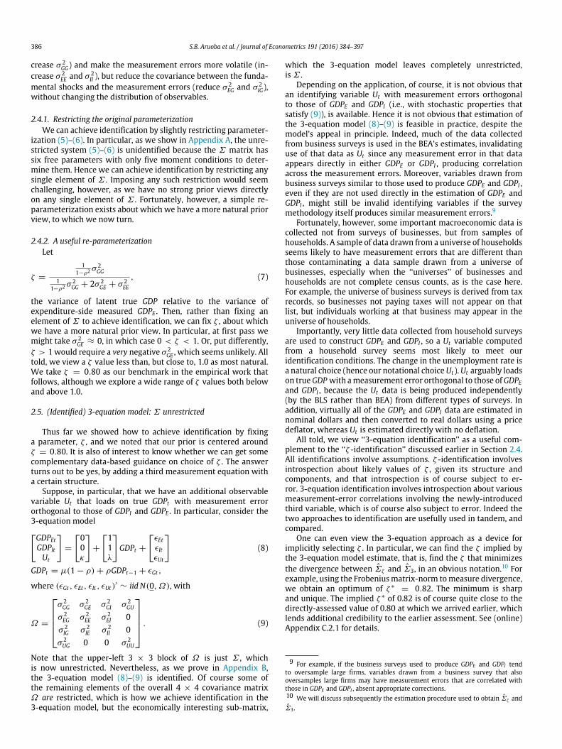
We report diagnostic normality checks in Fig. 2 for the threemodel shocks, ϵE , ϵI and ϵG. In the top panel we show the distri-butions of residual skewness across our 25,000 posterior draws.All are tightly and symmetrically distributed around zero, provid-

ing strong support for symmetry. In the middle panel we showthe distributions of residual kurtosis. Those for the measurementerrors ϵE and ϵI are tightly and symmetrically distributed aroundthree, consistent with normality. The distribution of residual kur-tosis for ϵG again appears consistent with normality, although lessstrongly than for the distributions of ϵE and ϵI . It is centered arounda median slightly greater than three, and it is skewed slightlyrightward.

As regards the white noise assumption, we show the interquar-tile ranges of our 25,000 posterior residual autocorrelation func-tion draws in the bottom panel of Fig. 2, again for each of ϵE , ϵI andϵG. They are tightly centered around zero and reveal no evidence ofserial correlation in measurement errors or true GDP innovations.

390 S.B. Aruoba et al. / Journal of Econometrics 191 (2016) 384–397

Fig. 2. Distributions of residual skewness, kurtosis and autocorrelations across 25,000 posterior draws. In the skewness and kurtosis plots the solid vertical lines denoteposterior medians. The shaded region in the autocorrelation plots denotes the posterior interquartile range.

All told, then, the GDPE and GDPI data appear to accord quite wellwith our benchmark dynamic factor model.

4. New perspectives on the properties of GDP

Our various extracted GDPM series differ in fundamental waysfromothermeasures, such asGDPE andGDPI . Herewediscuss someof the most important differences.

4.1. GDP sample paths

Let us begin by highlighting the sample-path differencesbetween our GDPM and the obvious competitors GDPE andGDPI . We make those comparisons in Fig. 3. In each panel we

show the sample path of GDPM together with a shaded pos-terior interquartile range, and we show one of the competitorseries.13 In the top panel we show GDPM vs. GDPE . There are of-ten wide divergences, with GDPE well outside the posterior in-terquartile range of GDPM . Indeed GDPE is substantially morevolatile than GDPM . In the bottom panel of Fig. 3 we show GDPMvs. GDPI . Noticeable divergences again appear often, with GDPIalso outside the posterior interquartile range of GDPM . The diver-gences are not as pronounced, however, and the ‘‘excess volatil-ity’’ apparent in GDPE is less apparent in GDPI . That is because,as we will show later, GDPM loads relatively more heavily onGDPI .

13 For GDPM we use our benchmark estimate from the 2-equation model withζ = 0.80.

S.B. Aruoba et al. / Journal of Econometrics 191 (2016) 384–397 391

Fig.

3.GD

Psamplepa

ths,19

60Q1–

2011

Q4.

Inea

chpa

nelw

esh

owthesamplepa

thof

GDP M

(ligh

tcolor)t

ogethe

rwith

posteriorinterqua

rtile

rang

ewith

shad

ingan

dwesh

owon

eof

theco

mpe

titor

series

(darkco

lor).F

orGD

P Mweus

eou

rben

chmarkestim

atefrom

the2-eq

uatio

nmod

elwith

ζ=

0.80

.

392 S.B. Aruoba et al. / Journal of Econometrics 191 (2016) 384–397

Fig. 4. GDP sample paths, 2007Q1–2009Q4. In each panel we show the sample path of GDPM (light color) together with posterior interquartile range with shading and weshow one of the competitor series (dark color). For GDPM we use our benchmark estimate from the 2-equation model with ζ = 0.80.

Table 3Priors and posteriors, 3-equation model, 1960Q1–2011Q4.

Parameter Prior Posterior(Mean, Std) 25% 50% 75%

µ N(3, 10) 2.60 2.78 2.95ρ N(0.3, 1) 0.54 0.58 0.63σ 2GG IG(10, 15) 6.73 6.96 7.35

σ 2GE N(0, 10) −1.27 −1.10 −0.84

σ 2GI N(0, 10) −1.03 −0.82 −0.59

σ 2EE IG(10, 15) 4.17 4.57 4.79

σ 2EI N(0, 10) 1.70 1.95 2.12

σ 2II IG(10, 15) 2.54 3.07 3.27

σ 2GU N(0, 10) 1.27 1.46 1.66

σ 2UU IG(0.3, 10) 0.50 0.59 0.71

κ N(0, 10) 1.53 1.62 1.71λ N(−0.5, 10) −0.55 −0.52 −0.50Posterior – −1251.1 −1249.6 −1248.3Likelihood – −1199.0 −1197.5 −1196.2

To emphasize the economic importance of the differences incompeting real activity assessments, in Fig. 4 we focus on thetumultuous period 2007Q1–2009Q4. The figure makes clear notonly that both GDPE and GDPI can diverge substantially from GDP ,but also that the timing and nature of their divergences can bevery different. In 2007Q3, for example, GDPE growth was stronglypositive and GDPI growth was negative.

4.2. GDP dynamics

In our linear framework, the data-generating process for trueGDPt is completely characterized by the pair, (σ 2

GG, ρ).14 In Fig. 5we

show those pairs across MCMC draws for all of our measurement-error models, and for comparison we show (ρ, σ 2) valuescorresponding to AR(1) models fit to GDPE alone and GDPI alone.In addition, in Table 1 we show a variety of statistics quantifyingthe sample properties of our various optimally extracted GDPM

14 We provide complementary nonlinear Markov-switching results in (online)Appendix C.2.3.

measures vs. those of GDPE , GDPI and GDPF , the forecast-error-based estimate of true GDP produced by Aruoba et al. (2012).

A key result of our analysis is the strong serial correlation(persistence, forecastability, etc.) of true GDP and our extractedGDPM , regardless of the particular specification. First consider the(ρ, σ 2

GG) draws, which determine the population autocovariancefunction of the true GDP process, depicted in Fig. 5. Depending onthe specification of the measurement error model, the posteriormean estimates of ρ lie in the interval of 0.5–0.6. For comparison,the estimated AR(1) coefficient for GDPE is only 0.33. The large ρvalues are accompanied by relatively small innovation variancesσ 2GG.Now consider the sample statistics of the extracted GDPM

series summarized in Table 1. As expected from the parameterestimates depicted in Fig. 5, the GDPM series is robustly moreserially correlated than GDPE , GDPI , GDPF . More specifically, if wefit an AR(1) model to GDPM we find that the shock persistence isroughly double that of GDPE (ρ of roughly 0.60 for GDPM vs. 0.30for GDPE). Simultaneously, the estimated innovation variances ofthe GDPM series are much smaller than those associated with therawdata. This translates intomuch higher predictive R2’s forGDPM .Indeed GDPM is twice as predictable as GDPI or GDPF , which inturn are twice as predictable as GDPE . Table 1 also reveals that thevariousGDPM series are all less volatile than each ofGDPE ,GDPI andGDPF , and a bit more skewed left.

To appreciate these results, consider the 2-equation modelwith block-diagonal Σ . A straightforward analysis of the impliedautocovariances implies that in population both GDPE and GDPIhave to be more volatile than true GDP . Moreover, due tothe presence of measurement errors that are independent ofthe GDP innovations, the first-order autocorrelations of GDPEand GDPI always provide downward-biased estimates of ρ, theautocorrelation of true GDP .

Oncewe allow for themeasurement errors to be correlatedwithϵGt , the volatility ranking and the sign of the bias are ambiguous.We can express the first-order autocorrelation of GDPE as

Corr(GDPEt ,GDPE,t−1) = ρV (GDPt) + σ 2

GE

V (GDPt) + 2σ 2GE + σ 2

EE. (19)

Thus the autocorrelation of GDPE provides an upward-biasedestimate of ρ if

σ 2GE > 2σ 2

GE + σ 2EE . (20)

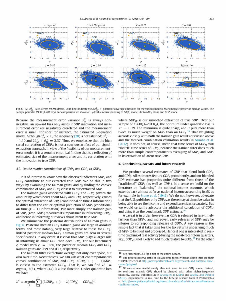
S.B. Aruoba et al. / Journal of Econometrics 191 (2016) 384–397 393

Fig. 5. (ρ, σ 2GG) Pairs across MCMC draws. Solid lines indicate 90% (σ 2

GG, ρ) posterior coverage ellipsoids for the various models. Stars indicate posterior median values. Thesample period is 1960Q1-2011.Q4. For comparison we show (σ 2, ρ) values corresponding to AR(1) models fit to GDPE alone and GDPI alone.

Because the measurement error variance σ 2EE is always non-

negative, an upward bias only arises if GDP innovation and mea-surement error are negatively correlated and the measurementerror is small. Consider, for instance, the estimated 3-equationmodel. Although σ 2

GE < 0, the inequality (20) is not satisfied: σ 2GE =

−1.10 and 2σ 2GE + σ 2

EE = 2.37. Thus, we emphasize that the highserial correlation of GDPM is not a spurious artifact of our signal-extraction approach. In view of the flexibility of ourmeasurement-error model, it is a genuine empirical finding that is a reflection ofestimated size of the measurement error and its correlation withthe innovation to true GDP .

4.3. On the relative contributions of GDPE and GDP I to GDPM

It is of interest to know how the observed indicators GDPE andGDPI contribute to our extracted true GDP . We do this in twoways, by examining the Kalman gains, and by finding the convexcombination of GDPE and GDPI closest to our extracted GDP .

The Kalman gains associated with GDPE and GDPI govern theamount by which news about GDPE and GDPI , respectively, causesthe optimal extraction of GDPt (conditional on time-t information)to differ from the earlier optimal prediction of GDPt (conditionalon time-(t − 1) information). Put more simply, the Kalman gainof GDPE (resp. GDPI ) measures its importance in influencing GDPM ,and hence in informing our views about latent true GDP .

We summarize the posterior distributions of Kalman gains inFig. 6. Posterior median GDPI Kalman gains are large in absoluteterms, and most notably, very large relative to those for GDPE .Indeed posterior median GDPE Kalman gains are zero in severalspecifications. In any event, it is clear that GDPI plays a larger rolein informing us about GDP than does GDPE . For our benchmarkζ -model with ζ = 0.80, the posterior median GDPI and GDPEKalman gains are 0.59 and 0.23, respectively.

The Kalman filter extractions average not only over space, butalso over time. Nevertheless, we can ask what contemporaneousconvex combination of GDPE and GDPI , λGDPE + (1 − λ)GDPI ,is closest to the extracted GDPM . That is, we can find λ∗

=

argminλ L(λ), where L(λ) is a loss function. Under quadratic losswe have

λ∗= argmin

λ

Tt=1

[(λGDPEt + (1 − λ)GDPIt) − GDPMt ]2 ,

where GDPMt is our smoothed extraction of true GDPt . Over oursample of 1960Q1–2011Q4, the optimum under quadratic loss isλ∗

= 0.29. The minimum is quite sharp, and it puts more thantwice as much weight on GDPI than on GDPE .15 That weightingaccords closely with both the Kalman gain results discussed aboveand the forecast-combination calibration results in Aruoba et al.(2012). It does not, of course, mean that time series of GDPM will‘‘match’’ time series of GDPF , because the Kalman filter does muchmore than simple contemporaneous averaging of GDPE and GDPIin its extraction of latent true GDP .

5. Conclusions, caveats, and future research

We produce several estimates of GDP that blend both GDPEand GDPI . All estimates feature GDPI prominently, and our blendedGDP estimate has properties quite different from those of the‘‘traditional’’ GDPE (as well as GDPI ). In a sense we build on theliterature on ‘‘balancing’’ the national income accounts, whichextends back almost as far as national income accounting itself, asfor example in Stone et al. (1942). We do not, however, advocatethat the U.S. publishes onlyGDPM , as theremay at times be value inbeing able to see the income and expenditure sides separately. Butwe would certainly advocate the additional calculation of GDPMand using it as the benchmark GDP estimate.16

A caveat is in order, however, as GDPI is released in less-timelyfashion than GDPE , and moreover, early releases of GDPI may beinferior to corresponding releases of GDPE . A key reason is thesimple fact that it takes time for the tax returns underlying muchof GDPI to be filed and processed. Hence if one is interested in real-time tracking of real activity (during themost-recent four quarters,say),GDPM is not likely to addmuch relative toGDPE .17 On the other

15 See Appendix C.2.2 for a plot of the entire surface.16 The Federal Reserve Bank of Philadelphia recently began doing this; see their‘‘GDPplus’’ series at http://www.philadelphiafed.org/research-and-data/real-time-center/gdpplus/.17 Of course one would surely also not want to use GDPE alone. Instead,for real-time analysis GDPE should be blended with other higher-frequency(monthly, weekly) indicators as in Aruoba et al. (2009) and Aruoba and Diebold(2010), implemented in real time by the Federal Reserve Bank of Philadelphiaat http://www.philadelphiafed.org/research-and-data/real-time-center/business-conditions-index.

394 S.B. Aruoba et al. / Journal of Econometrics 191 (2016) 384–397

Fig. 6. (KGE , KGI ) Pairs across MCMC draws. Solid lines indicate 90% posterior coverage ellipsoids. Stars indicate posterior median values.

hand, whether one uses up-to-the-instant GDP data, as opposed toup-to-a-year-ago data, is typically irrelevant to the research workfor which we seek to contribute a superior input.

Interesting extensions of our framework and methods arepossible. Consider, for example, forecasting. When forecastinga ‘‘traditional’’ GDP series such as GDPE , we must take it asgiven (i.e., we must ignore measurement error). The analogousprocedure in our framework would take GDPM as given, modelingand forecasting it directly, ignoring the fact that it is only anestimate. Fortunately, however, in our framework we need notdo that. Instead we can estimate and forecast directly from thedynamic factor model, accounting for all sources of uncertainty,which should translate into superior interval and density forecasts.Related, it would be interesting to calculate directly the point,interval and density forecast functions corresponding to ourmeasurement-error model.

Acknowledgments

We are grateful to the Editor (William Barnett) and twoanonymous referees for insightful comments that improved thepaper significantly. For helpful comments we are also gratefulto Bob Chirinko, Rob Engle, Graham Elliott, Don Harding, JohnHaltiwanger, Andrew Harvey, Jan Jacobs, Greg Mankiw, AdrianPagan, John Roberts, Matt Shapiro, Neil Shephard, Minchul Shin,Chris Sims, Mark Watson, Justin Wolfers and Simon van Norden.For research support we thank the National Science Foundationand the Real-Time Data Research Center at the Federal ReserveBank of Philadelphia.

Appendix

Here we report various details of theory, establishing identifi-cation results for the two- and three-variable models in Appen-dices A and B, respectively. The identification analysis is basedon Komunjer and Ng (2011).

Appendix A. Identification in the two-equation model

The constants in the state-space model can be identifiedfrom the means of GDPEt and GDPIt . To simplify the subsequent

exposition we now set the constant terms to zero:

GDPt = ρGDPt−1 + ϵGt (A.1)GDPEtGDPIt

=

11

GDPt +

ϵEtϵIt

(A.2)

and the joint distribution of the errors is

ϵt =

ϵGtϵEtϵIt

∼ iidN

0, Σ

, where Σ =

ΣGG · ·

ΣEG ΣEE ·

ΣIG ΣIE ΣII

.

Using thenotation inKomunjer andNg (2011),wewrite the systemas

st+1 = A(θ)st + B(θ)ϵt+1 (A.3)

yt+1 = C(θ)st + D(θ)ϵt+1, (A.4)

where

st = GDPt , yt =

GDPEtGDPIt

(A.5)

A(θ) = ρ, B(θ) =1 0 0

C(θ) =

ρρ

, D(θ) =

1 1 01 0 1

and θ = [ρ, vech(Σ)′]′. Note that only A(θ) and C(θ) are non-trivial functions of θ .

Assumption 1. The parameter vector θ satisfies the followingconditions: (i) Σ is positive definite; (ii) 0 ≤ ρ < 1.

Because the rows ofD are linearly independent, Assumption 1(i)implies that DΣD′ is non-singular. In turn, we deduce thatAssumptions 1, 2, and 4-NS of Komunjer and Ng (2011) aresatisfied.

We now express the state-space system in terms of itsinnovation representation

st+1|t+1 = A(θ)st|t + K(θ)at+1 (A.6)yt+1 = C(θ)st|t + at+1,

where at+1 is the one-step-ahead forecast error of the systemwhose variance we denote by Σa(θ). The innovation representa-tion is obtained from the Kalman filter as follows. Suppose that

S.B. Aruoba et al. / Journal of Econometrics 191 (2016) 384–397 395

conditional on time t information Y1:t the distribution of st |Y1:t ∼

N(st|t , Pt|t). Then the joint distribution of [st+1, y′

t+1]′ is

st+1yt+1

Y1:T ∼

Ast|tCst|t

,

APt|tA′

+ BΣB′ APt|tC ′+ BΣD′

CPt|tA′+ DΣB′ CPt|tC ′

+ DΣD′

.

In turn, the conditional distribution of st+1|Y1:t+1 is

st+1|Y1:t+1 ∼ Nst+1|t+1, Pt+1|t+1

,

where

st+1|t+1 = Ast|t + (APt|tC + BΣD′)(CPt|tC ′+ DΣD′)−1(yt − Cst|t)

Pt+1|t+1 = APt|tA′+ BΣB′

− (APt|tC ′+ BΣD′)

× (CPt|tC ′+ DΣD′)−1(CPt|tA′

+ DΣB′).

Now let P be the matrix that solves the Riccati equation,

P = APA′+ BΣB′

− (APC ′+ BΣD′)(CPC ′

+ DΣD′)−1

× (CPA′+ DΣB′), (A.7)

and let K be the Kalman gain matrix

K = (APC ′+ BΣD′)(CPC ′

+ DΣD′)−1. (A.8)

Then the one-step-ahead forecast error matrix is given by

Σa = CPC ′+ DΣD′. (A.9)

Eqs. (A.7)–(A.9) determine the matrices that appear in theinnovation-representation of the state-space system (A.6).

In order to be able to apply Proposition 1-NS of Komunjer andNg (2011) we need to express P , K , and Σa in terms of θ . Whilesolving Riccati equations analytically is in general not feasible,our system is scalar, which simplifies the calculation considerably.Replacing A by ρ and P by p such that scalars appear in lower case,and defining

ΣBB = BΣB′, ΣBD = BΣD′, and ΣDD = DΣD′,

we can write (A.7) as

p = pρ2+ ΣBB − (pρC ′

+ ΣBD)(pCC ′+ ΣDD)

−1

× (pρC + ΣDB). (A.10)

Likewise,

K = (pρC ′+ ΣBD)(pCC ′

+ ΣDD)−1 and

Σa = pCC ′+ ΣDD.

(A.11)

Because ΣBB − ΣBDΣ′

DDΣDB > 0 we can deduce that p > 0.Moreover, because A = ρ ≥ 0 and C ≥ 0, we deduce thatK = 0 and therefore Assumption 5-NS of Komunjer and Ng (2011)is satisfied. According to Proposition 1-NS in Komunjer and Ng(2011), two vectors θ and θ1 are observationally equivalent if andonly if there exists a scalar γ = 0 such that

A(θ1) = γ A(θ)γ −1 (A.12)

K(θ1) = γK(θ) (A.13)

C(θ1) = C(θ)γ −1 (A.14)

Σa(θ1) = Σa(θ). (A.15)

Define θ = [ρ, vech(Σ)′]′ and θ1 = [ρ1, vech(Σ1)′]′. Using the

definition of the scalar A(θ) in (A.5) we deduce from (A.12) thatρ1 = ρ. Since C(θ) depends on θ only through ρ we can deducefrom (A.14) that γ = 1. Thus, given θ and ρ, the elements of thevector vech(Σ1)have to satisfy conditions (A.13) and (A.15),which,using (A.11), can be rewritten as

Σa = Σa1 = p1CC ′+ ΣDD1 (A.16)

K = K1 = (p1ρC ′+ ΣBD1)Σ

−1a . (A.17)

Moreover, p1 has to solve the Riccati equation (A.10):

p1 = p1ρ2+ ΣBB1 − K0(p1ρC + ΣBD). (A.18)

Eqs. (A.16)–(A.18) are satisfied if and only if

pCC ′+ ΣDD = p1CC ′

+ ΣDD1 (A.19)

pρC ′+ ΣBD = p1ρC ′

+ ΣBD1 (A.20)

p(1 − ρ2) − ΣBB = p1(1 − ρ2) − ΣBB1. (A.21)We proceed by deriving expressions for the Σxx matrices that

appear in (A.19)–(A.21):ΣBB = ΣGG

ΣBD =ΣGG + ΣGE ΣGG + ΣGI

ΣDD =

ΣGG + ΣEE + 2ΣEG ·

ΣGG + ΣGE + ΣGI + ΣEI ΣGG + ΣII + 2ΣGI

.

Without loss of generality let

ΣGG1 = ΣGG + (1 − ρ2)δ, (A.22)which implies thatΣBB1 = ΣBB + (1 − ρ2)δ.

We now distinguish the cases δ = 0 and δ = 0.Case 1: δ = 0. (A.21) implies p1 = p. It follows from (A.20) thatΣBD1 = ΣBD. In turn, ΣGE1 = ΣGE and ΣGI1 = ΣGI . Finally,to satisfy (A.19) it has to be the case that ΣDD1 = ΣDD, whichimplies that the remaining elements ofΣ andΣ1 are identical. Weconclude that θ1 = θ .Case 2: δ = 0. (A.21) implies p1 = p + δ. Now consider (A.20):pρC ′

+ ΣBD = pρ2 1 1

+

ΣGG + ΣGE ΣGG + ΣGI

!= pρ2

1 1+ δρ2

1 1

+ΣGG + ΣGE1 ΣGG + ΣGI1

+ δ(1 − ρ2)

1 1

.

We deduce thatΣGE1 = ΣGE − δ, ΣGI1 = ΣGI − δ. (A.23)Finally, consider (A.19), which can be rewritten as0 = ΣDD1 − ΣDD + δCC ′.

Using the previously derived expressions for ΣDD and ΣDD1 weobtain the following three conditions0 = (1 − ρ2)δ + (ΣEE1 − ΣEE) − 2δ + ρ2δ = ΣEE1 − ΣEE − δ

0 = (1 − ρ2)δ − 2δ + (ΣEI1 − ΣEI) + ρ2δ = ΣEI1 − ΣEI − δ

0 = (1 − ρ2)δ + (ΣII1 − ΣII) − 2δ + ρ2δ = ΣII1 − ΣII − δ.

Thus, we deduce that

ΣEE1 = ΣEE + δ, ΣEI1 = ΣEI + δ, andΣII1 = ΣII + δ.

(A.24)

Combining (A.22)–(A.24) we find that

Σ1 =

ΣGG + δ(1 − ρ2) ΣGE − δ ΣGI − δΣGE − δ ΣEE + δ ΣEI + δΣGI − δ ΣEI + δ ΣII + δ

. (A.25)

Thus, we have proved the following theorem:

396 S.B. Aruoba et al. / Journal of Econometrics 191 (2016) 384–397

ΣBB = ΣGG

ΣBD =ΣGG + ΣGE ΣGG + ΣGI λΣGG + ΣGU

ΣDD =

ΣGG + ΣEE + 2ΣGE · ·

ΣGG + ΣGE + ΣGI + ΣEI ΣGG + ΣII + 2ΣGI ·

λΣGG + λΣGE + ΣGU λΣGG + λΣGI + ΣGU λ2ΣGG + 2λΣGU + ΣUU

Box I.

Theorem A.1. Suppose Assumption 1 is satisfied. Then the two-variable model is

(i) identified if Σ is diagonal as in Section 2.1;(ii) identified if Σ is block-diagonal as in Section 2.2;(iii) not identified if Σ is unrestricted as in Section 2.3;(iv) identified if Σ is restricted as in Section 2.4.

Appendix B. Identification in the three-equation model

The identification analysis of the three-variable is similar to theanalysis of the two-variable model in the previous section. Thesystem is given by

GDPt = ρGDPt−1 + ϵGt (B.26)GDPEtGDPItUt

=

11λ

GDPt +

ϵEtϵItϵUt

, (B.27)

and the joint distribution of the errors is

ϵt =

ϵGtϵEtϵItϵUt

∼ iidN0, Σ

,

where Σ =

ΣGG · · ·

ΣEG ΣEE · ·

ΣIG ΣIE ΣII ·

ΣUG ΣUE ΣUI ΣUU

.

The matrices A(θ), B(θ), C(θ), and D(θ) are now given by

A(θ) = ρ, B(θ) =1 0 0 0

C(θ) =

ρρλρ

, D(θ) =

1 1 0 01 0 1 0λ 0 0 1

,

where θ = [ρ, λ, vech(Σ)′]′.

Assumption 2. The parameter vector θ satisfies the followingconditions: (i) Σ is positive definite; (ii) 0 < ρ < 1; (iii) λ = 0;(iv) ΣUE = ΣUI = 0.

Condition (A.12) implies that ρ1 = ρ. Moreover, (A.14) impliesthat γ = 1 and that λ1 = λ provided that ρ = 0. As for the two-variable model, we have to verify that (A.19)–(A.21) are satisfied.The matrices Σxx that appear in these equations are given in Box I.

Without loss of generality, let

ΣGG,1 = ΣGG + (1 − ρ2)δ,

which implies that

ΣBB,1 = ΣBB + (1 − ρ2)δ.

Case 1: δ = 0. (A.21) implies p1 = p. It follows from (A.20)that ΣBD,1 = ΣBD. In turn, ΣGE,1 = ΣGE , ΣGI,1 = ΣGI , andΣGU,1 = ΣGU . Finally, to satisfy (A.17) it has to be the case thatΣDD,1 = ΣDD, which implies that the remaining elements of Σ

and Σ1 are identical for the two parameterizations. We concludethat it has to be the case that θ1 = θ .

Case 2: δ = 0. (A.21) implies p1 = p + δ. Now consider (A.20):

pρC ′+ ΣBD

= pρ2 1 1 λ

+

ΣGG + ΣGE ΣGG + ΣGI λΣGG + ΣGU

!= pρ2

1 1 λ+ δρ2

1 1 λ

+ΣGG + ΣGE,1 ΣGG + ΣGI,1 λΣGG + ΣGU,1

+ (1 − ρ2)δ

1 1 λ

.

We deduce that

ΣGE,1 = ΣGE − δ, ΣGI,1 = ΣGI − δ, ΣGU,1 = ΣGU − δ.

Finally, consider (A.19), which can be rewritten as

0 = ΣDD,1 − ΣDD + δCC ′.

Using the previously derived expressions for ΣDD and ΣDD1 weobtain the following five conditions

0 = (1 − ρ2)δ + (ΣEE1 − ΣEE) − 2δ + ρ2δ = ΣEE1 − ΣEE − δ

0 = (1 − ρ2)δ − 2δ + (ΣEI1 − ΣEI) + ρ2δ = ΣEI1 − ΣEI − δ

0 = (1 − ρ2)δ + (ΣII1 − ΣII) − 2δ + ρ2δ = ΣII1 − ΣII − δ

0 = λ(1 − ρ2)δ − λδ − δ + λρ2δ = δ

0 = λ2(1 − ρ2)δ − 2λδ + (ΣUU1 − ΣUU) + λ2ρ2δ

= ΣUU1 − ΣUU − λ(2 − λ)δ.

Thus, we deduce that

δ = 0, ΣEE1 = ΣEE, ΣEI1 = ΣEI , ΣII1 = ΣII ,

and ΣUU1 = ΣUU .

This proves the following theorem:

Theorem B.1. Suppose Assumption 2 is satisfied. Then the three-variable model is identified.

Appendix C. Supplementary data

Supplementary material related to this article can be foundonline at http://dx.doi.org/10.1016/j.jeconom.2015.12.009.

References

Aruoba, B., 2008. Data revisions are not well-behaved. J. Money Credit Bank. 40,319–340.

Aruoba, S.B., Diebold, F.X., 2010. Real-time macroeconomic monitoring: Realactivity, inflation, and interactions. Am. Econ. Rev. 100, 20–24.

Aruoba, S.B., Diebold, F.X., Nalewaik, J., Schorfheide, F., Song, D., 2012. ImprovingGDP measurement: A forecast combination perspective. In: Chen, X., Swan-son, N. (Eds.), Recent Advances and Future Directions in Causality, Prediction,and Specification Analysis: Essays in Honour of Halbert L. White Jr., Springer,pp. 1–26.

Aruoba, S.B., Diebold, F.X., Scotti, C., 2009. Real time measurement of businessconditions. J. Bus. Econom. Statist. 27, 417–427.

BEA 2006. A Guide to the National Income and Product Accounts of the UnitedStates. Bureau of Economic Analysis, Washington, DC.http://www.bea.gov/national/pdf/nipaguid.pdf.

Durbin, J., Koopman, S.J., 2001. Time Series Analysis by State SpaceMethods. OxfordUniversity Press, Oxford.

Edwards, C.L., Howrey, E.P., 1991. A ‘true’ time series and its indicators: Analternative approach. J. Amer. Statist. Assoc. 86, 878–882.

S.B. Aruoba et al. / Journal of Econometrics 191 (2016) 384–397 397

Faust, J., Rogers, J.H.,Wright, J.H., 2005. News and noise in G-7GDP announcements.J. Money Credit Bank. 37, 403–417.

Fixler, D.J., Nalewaik, J.J., 2009. News, Noise, and Estimates of the True UnobservedState of the Economy. Bureau of Labor Statistics and Federal Reserve Board,Manuscript.

Fleischman, C.A., Roberts, J.M., 2011. A Multivariate Estimate of Trends and Cycles.Federal Reserve Board, Manuscript.

Gartaganis, A.J., Goldberger, A.S., 1955. A note on the statistical discrepancy in thenational accounts. Econometrica 23, 166–173.

Geweke, J.F., 1977. The dynamic factor analysis of economic time series models.In: Aigner, D., Goldberger, A. (Eds.), Latent Variables in Socioeconomic Models.North Holland, pp. 365–383.

Greenaway-McGrevy, Ryan, 2011. Is GDP or GDI a better measure of output? Astatistical approach. Bureau of Economic Analysis Manuscript.

Harding, D., Scutella, R., (1996). Efficient Estimates of GDP, Unpublished SeminarNotes, La Trobe University, Australia.

Jacobs, J.P.A.M., van Norden, S., 2011. Modeling data revisions: Measurement errorand dynamics of true values. J. Econometrics 161, 101–109.

Kishor, N.K., Koenig, E.F., 2012. VAR estimation and forecasting when data aresubject to revision. J. Bus. Econom. Statist. 30 (2), 181–190.

Komunjer, I., Ng, S., 2011. Dynamic identification of dynamic stochastic generalequilibrium models. Econometrica 79, 1995–2032.

Landefeld, J.S., Seskin, E.P., Fraumeni, B.M., 2008. Taking the pulse of the economy:Measuring GDP. J. Econ. Perspect. 22, 193–216.

Mankiw, N.G., Runkle, D.E., Shapiro, M.D., 1984. Are preliminary announcements ofthe money stock rational forecasts? J. Monetary Econ. 14, 15–27.

Mankiw, N.G., Shapiro, M.D., 1986. News or noise: An analysis of GNP revisions.Survey of Current Business 20–25.

McCulla, S.H., Smith, S., 2007. Measuring the Economy: A Primer on GDP andthe National Income and Product Accounts. Bureau of Economic Analysis,Washington, DC. http://www.bea.gov/national/pdf/nipa_primer.pdf.

Nalewaik, J.J., 2010. The income- and expenditure-side estimates of U.S. outputgrowth. Brookings Papers on Economic Activity 1, 71–127 (with discussion).

Rassier, D.G., 2012. The role of profits and income in the statistical discrepancy.Survey of Current Business 8–22.

Sargent, T.J., Sims, C.A., 1977. Business cycle modeling without pretending to havetoo much a priori theory. In: Sims, C.A. (Ed.), New Methods in Business CycleResearch: Proceedings fromaConference. Federal Reserve Bank ofMinneapolis,pp. 45–109.

Smith, R.J., Weale, M.R., Satchell, S.E., 1998. Measurement error with accountingconstraints: Point and interval estimation for latent data with an application toU.K. gross domestic product. Rev. Econom. Stud. 65, 109–134.

Stone, R., Champernowne, D.G., Meade, J.E., 1942. The precision of national incomeestimates. Rev. Econom. Stud. 9, 111–125.

Watson, M.W., Engle, R.F., 1983. Alternative algorithms for the estimationof dynamic factor, MIMIC and varying coefficient regression models.J. Econometrics 23, 385–400.