Journal of Wind Engineering & Industrial Aerodynamics 169 (2017) 168–176

Contents lists available at ScienceDirect

Journal of Wind Engineering & Industrial Aerodynamics

journal homepage: www.elsevier .com/locate/ jweia

Aerodynamic roughness parameters in cities: Inclusion of vegetation

Christoph W. Kent a,*, Sue Grimmond a, David Gatey b

a Department of Meteorology, University of Reading, Reading, United Kingdomb Risk Management Solutions, London, United Kingdom

A R T I C L E I N F O

Keywords:Aerodynamic roughness lengthDrag coefficient for vegetationLogarithmic wind profileMorphometric methodUrbanZero-plane displacement

* Corresponding author. Room 2U08, Department of ME-mail addresses: C.W.Kent@pgr.reading.ac.uk, c.s.grim

http://dx.doi.org/10.1016/j.jweia.2017.07.016Received 15 December 2016; Received in revised form 24

0167-6105/© 2017 The Authors. Published by Elsevier L

A B S T R A C T

A widely used morphometric method (Macdonald et al. 1998) to calculate the zero-plane displacement (zd) andaerodynamic roughness length (z0) for momentum is further developed to include vegetation. The adaptation alsoapplies to the Kanda et al. (2013) morphometric method which considers roughness-element height variability.Roughness-element heights (mean, maximum and standard deviation) of both buildings and vegetation arecombined with a porosity corrected plan area and drag formulation. The method captures the influence ofvegetation (in addition to buildings), with the magnitude of the effect depending upon whether buildings orvegetation are dominant and the porosity of vegetation (e.g. leaf-on or leaf-off state). Application to five urbanareas demonstrates that where vegetation is taller and has larger surface cover, its inclusion in the morphometricmethods can be more important than the morphometric method used. Implications for modelling the logarithmicwind profile (to 100 m) are demonstrated. Where vegetation is taller and occupies a greater amount of space,wind speeds may be slowed by up to a factor of three.

1. Introduction

During neutral atmospheric stratification, the mean wind speed (Uz)at a height z, above a surface can be estimated using the logarithmic windlaw (Tennekes, 1973):

Uz ¼ u*κln�z� zdz0

�(1)

where u* is the friction velocity, κ ~ 0.40 (H€ogstr€om, 1996) is vonKarman's constant, z0 is the aerodynamic roughness length, and zd is thezero-plane displacement. The aerodynamic roughness parameters (zd andz0) can be related to surface geometry using morphometric methods (e.g.Grimmond and Oke, 1999; Kent et al., 2017a).

Uncertainties in wind-speed estimations arise from using idealisedwind-speed profile relations, as well as representing the surface usingonly two roughness parameters (zd and z0), which are based upon asimplification of surface geometry. Both observations and physical ex-periments are therefore critical to assess the most appropriate methods todetermine roughness parameters and for wind-speed estimation (e.g.Cheng et al., 2007; Tieleman 2008; Drew et al., 2013). Using the loga-rithmic wind law (Eq. (1)), Kent et al. (2017a) demonstrate that windspeeds estimated up to 200 m above the canopy in central London (UK)

eteorology, University of Reading, Eamond@reading.ac.uk (C.W. Kent).

July 2017; Accepted 24 July 2017

td. This is an open access article und

most resemble observations using morphometric methods which accountfor roughness-element height variability (specifically, the Mill-ward-Hopkins et al., 2011 and Kanda et al., 2013 methods). However, anuncertainty of >2.5 m s�1 exists (>25% of the mean wind speed) due tothe flow variability throughout the profile (Kent et al., 2017a;their Fig. 7).

Bluff bodies (e.g. buildings) and porous roughness elements (e.g.vegetation) have different influences upon wind flow (Taylor, 1988;Finnigan, 2000; Guan et al., 2000, 2003) which need to be accounted for.Althoughmorphometric methods have been developed for only buildings(examples in Mohammad et al., 2015) or vegetated canopies (e.g. Nakaiet al., 2008), existing morphometric methods do not consider both solidand porous bodies (i.e. vegetation) in combination.

With the intention of collectively considering buildings and vegeta-tion to determine zd and z0, this work develops the widely-used Mac-donald et al. (1998, hereafter Mac) morphometric method to includevegetation. The development applies to the more recently proposedKanda et al. (2013, hereafter Kan) development of Mac which considersroughness-element height variability. The implications for estimating thelogarithmic wind-speed profile (Eq. (1)) up to 100 m above five differenturban surfaces are discussed.

rley Gate, PO Box 243, Reading, RG6 6BB, United Kingdom.

er the CC BY license (http://creativecommons.org/licenses/by/4.0/).

Notation

A*f Unsheltered frontal area of roughness elements

a0, b0, c0, a1, b1, c1Kanda et al. (2013) method constants

Af Frontal area of roughness elementsAp Plan area of roughness elementsAT Total surface areaCD Drag coefficientFD Total drag of roughness elementsHav Average roughness-element heightHmax Maximum roughness-element heightκ von Karman's constant ¼ 0.4 (H€ogstr€om, 1996)L Obukhov length ¼ � Tu*3

kgw'T '

P2D Two-dimensional porosityP3D Three-dimensional or aerodynamic porosityPv ratio of CDv to CDb

u* Friction velocity ¼ ðð�u'w'Þ2 þ ð�v'w'Þ2Þ0:25 ¼ ffiffiffiffiffiffiτ=ρ

qUz Wind speed at height zz0 Aerodynamic roughness lengthzd Zero-plane displacementα zd correction coefficient (Macdonald et al., 1998)

β Drag correction coefficient (Macdonald et al., 1998)λf Frontal area index of roughness elementsλf-crit Frontal area index for peak z0λp Plan area index of roughness elementsρ Density of airσH Standard deviation of roughness-element heightsσv Standard deviation of lateral wind velocity (crosswind)τ Surface shear stress

AbbreviationsCC_hv City centre with high vegetationCC_lv City centre with low vegetationKan Kanda et al. (2013) morphometric methodMac Macdonald et al. (1998) morphometric methodPa Urban parkSB_hv Suburban area with high vegetationSB_lv Suburban area with low vegetation

Additional subscriptsb Buildingsv Vegetationl-on Leaf-onl-off Leaf-off

C.W. Kent et al. Journal of Wind Engineering & Industrial Aerodynamics 169 (2017) 168–176

2. Methodology

2.1. Macdonald et al. and Kanda et al. Morphometric methods

Morphometric methods traditionally characterise roughness elementsby their average height (Hav), plan area index (λp) and frontal area index(λf). The λp is the ratio of the horizontal area occupied by roughness el-ements (‘roof’ or vegetative canopy, Ap) to total area under consideration(AT), whereas λf is the area of windward vertical faces of the roughnesselements (Af) to AT. By including the standard deviation (σH) andmaximum (Hmax) roughness-element heights, newer methods considerheight variability (Millward-Hopkins et al., 2011; Kanda et al., 2013).

The Mac method is derived from fundamental principles and withoutassumptions about wake effects and recirculation zones of solid rough-ness elements (Macdonald et al., 1998), which vary for porous elements(Wolfe and Nickling, 1993; Judd et al., 1996; Sutton and McKennaNeuman, 2008; Suter-Burri et al., 2013). The formulation of zd and z0 is(Macdonald et al., 1998):

Maczd ¼�1þ α�λp

�λp � 1

� �Hav (2)

Macz0 ¼��

1� zdHav

�exp

��0:5β

CDb

κ2

�1� zd

Hav

�λf�0:5 ��

Hav (3)

where the constant, α, is used to control the increase in zd with λp, a dragcorrection coefficient, β, is used to determine z0 and CDb is the drag co-efficient for buildings. Coefficients can be fitted to observations. Forexample, using Hall et al.'s (1996) wind tunnel data, Macdonald et al.(1998) recommend CDb ¼ 1.2 and α ¼ 4.43, β ¼ 1.0 for staggered arrays;and α ¼ 3.59, β ¼ 0.55 for square arrays. The staggered array values andCDb ¼ 1.2 are used here.

Using large eddy simulations for real urban districts of Japan, Kandaet al. (2013) argue that the upper limit of zd is Hmax and therefore:

Kanzd ¼hcoX2 þ

�ao λpbo � co

XiHmax;

X ¼ σH þ Hav

Hmax

(4)

and

169

Kanz0 ¼�b1Y2 þ c1Y þ a1

�Macz0 ;

Y ¼ λp σHHav

(5)

where 0� X� 1, 0� Y and a0, b0, c0, a1, b1 and c1 are regressed constantswith values: 1.29, 0.36, �0.17, 0.71, 20.21 and �0.77, respectively.

2.2. Considering vegetation

Although, consideration has been given to treatment of vegetationwithin building-based morphometric methods (e.g. a reduction of height,Holland et al., 2008), the flexibility, structure and porosity of vegetationsuggest the effects upon wind flow and aerodynamic roughness are morecomplex (Finnigan, 2000; Nakai et al., 2008). During the methoddevelopment proposed here, vegetation porosity is used, as it is the mostcommon descriptor of the internal structure (Heisler and Dewalle, 1988)and relatively easy to determine (Guan et al., 2002; Crow et al., 2007;Yang et al., 2017). Unlike other characteristics (e.g. structure or flexi-bility), porosity can be generalised across vegetation types or specieswith values between 0 (completely impermeable) and 1 (completelyporous). Optical (P2D) and volumetric/aerodynamic (P3D) porosity can berelated to each other: P3D ¼ P2D0.40 (Guan et al., 2003), P3D ¼ P2D0.36 (Grantand Nickling, 1998).

The drag of vegetation is also considered, which through absorbingmomentum from the wind (Finnigan, 2000; Guan et al., 2003; Krayenhoffet al., 2015) can significantly reduce the surface shear stress (τ) (Wolfeand Nickling, 1993), as well as reduce the exchange between in-canopyand above-canopy flow (Gromke and Ruck, 2009; Vos et al., 2013).The drag generated by vegetation (Wyatt and Nickling, 1997; Grant andNickling, 1998; Gillies et al., 2000, 2002; Guan et al., 2003) and otherporous structures (Seginer, 1975; Jacobs, 1985; Taylor, 1988) variesfrom that of a solid structure with similar geometry. This variation ismore complex than can be resolved by a simple reduction of the frontalarea (e.g. Taylor, 1988; Guan et al., 2003). Therefore, the changes in dragare directly considered using the drag coefficient.

Typically, morphometric methods use a single drag coefficient forbuildings (CDb), whereas here the drag coefficient of vegetation (CDv) isalso used. The nature and type of vegetation (e.g. size, structure,

Fig. 1. Relation between the drag coefficient of porous roughness elements (CDv) andporosity (P3D), data from: Hagen and Skidmore (1971) (HA); Wilson (1985) (WI); Seginer(1975) (SG); Grant and Nickling (1998) (GN); Bitog et al. (2011) (BI), Guan et al. (2000)(GU00) and Guan et al. (2003) (GU03). Lines are relations from Guan et al. (2003) (GUwb,Eq. (6)) and Guan et al. (2000) (GUit, Eq. (7)).

C.W. Kent et al. Journal of Wind Engineering & Industrial Aerodynamics 169 (2017) 168–176

flexibility, leaf type) affect CDv (Rudnicki et al., 2004). In addition,sheltering and the reconfiguration of shape and leaf orientation undervarying flow characteristics means a single value for CDv may be inap-propriate (e.g. Guan et al., 2000, Guan et al., 2003; Vollsinger et al.,2005; Pan et al., 2014). Although attempts have been made to separatethe form and viscous components of vegetation drag (e.g. Shaw andPatton, 2003), the components tend to be considered in combination(CDv), as is done here.

The CDv of foliage typically varies between 0.1 and 0.3 (Katul et al.,2004). From large eddy simulations, Shaw and Schumann (1992) and Suet al. (1998) propose CDv ¼ 0.15. Other numerical simulations suggestCDv ¼ 0.25 (da Costa et al., 2006) and CDv ¼ 0.2 (Zeng and Takahashi,2000) for pine forests. Field studies in boreal canopies (pine, aspen andspruce) indicate CDv varies between 0.1 and 0.3 (Amiro, 1990). A CDv of0.2 is commonly used in numerical studies of wind flow in vegetatedcanopies (Van Renterghem and Botteldooren, 2008). Whereas, rough-and smooth-surface cylinders have CD¼ 1.2 (Simiu and Scanlan, 1996) orCD ¼ 0.8 (Guan et al., 2000), respectively.

There is evidence that that CDv varies with wind speed, with higherCDv at lower wind speeds. Results from wind tunnel studies include: forseven 5.8–8.5 m British forest saplings CDv varied from 0.88 to 0.15 whenwind speeds were between 9 and 26 m s�1 (Mayhead, 1973); for2.5–5.0 m tall conifer saplings with wind speeds between 4 and 20 m s�1

CDv varied between 1.5 and 0.2 (Rudnicki et al., 2004); and, for fivehardwood species CDv varied between 1.02 and 0.10 (Vollsinger et al.,2005). Conclusions are similar in the field, where Koizumi et al. (2010)report CDv for three poplar tree crowns varying from 1.1 to 0.1 with windspeeds between 1 and 15 m s�1. These results indicate at high windspeeds the relative drag of an individual tree (CDv ~ 0.1–0.2) is smallcompared to that of buildings, but during some flow conditions CDv canapproach that of a solid structure of similar shape (i.e. 1.2) and thereforeexert similar drag to buildings.

The state of foliage on a tree (i.e. porosity) influences the amount ofdrag exerted on the flow. Koizumi et al.'s (2010) field observations atwind speeds of 10 m s�1 found CDv to over halve when tree crowns aredefoliated (i.e. more porous). Current understanding of CDv variabilitywith porosity is based upon artificial (i.e. two-dimensional) and natural(i.e. tree or tree model) wind break studies. Hagen and Skidmore (1971)found CDv to be similar to single tree values: CDv ~ 0.5 for one row de-ciduous windbreaks and CDv ~ 0.6–1.2 for coniferous windbreaks. Guanet al.'s (2003, their Table 5) synthesis of CDv for two-dimensional struc-tures or naturally vegetated windbreaks of varying porosity provides arelation between CDv and porosity (P3D):

CDv ¼ 1:08�1 � P3D

1:8�

(6)

Similarly, for an isolated model tree, Guan et al. (2000) show:

CDv ¼ �1:251P3D2 þ 0:489P3D þ 0:803 (7)

Results of previous studies (summarised in Fig. 1) indicate that moreimpermeable roughness elements (i.e. P3D ¼ 0) tend to have the largestCDv, approaching that of a solid structure (0.8–1.2). As aerodynamicporosity increases, CDv decreases approximately as a power function tozero for an open surface (i.e. P3D ¼ 1). Observations by Grant andNickling (1998) for a single conifer tree (Fig. 1, GN) and wind tunnelstudies by Guan et al. (2000) support evidence that the relation may peakat critical porosities (Grant and Nickling, 1998; Gillies et al., 2002).

2.3. Parameter determination and method development

In the methodology proposed here, the Hav, Hmax and σH of allroughness elements (i.e. buildings and vegetation) are determined.

Porosity is accounted for when determining λp as vegetation hasopenings in the volume it occupies. The plan area of vegetation (Apv) isreduced by a porosity factor (i.e. 1 – P3D). The λp of both buildings and

170

porous vegetation becomes:

λp ¼Pn

i¼1Apbi þPn

j¼1ð1� P3DÞApvj

AT(8)

where Apb is the plan area of buildings and i or j refers to each individualbuilt or vegetated roughness element, respectively.

TheMacmethod (Sect. 2.1) considers the drag balance at the top of agroup of homogeneous roughness elements (of height z) approached by alogarithmic wind profile. If the roughness elements are of variableheight, z is replaced by their average height (Hav) (Macdonald et al.,1998). Numerical models demonstrate the relative impact of trees andbuildings represented by the drag coefficient are not affected by eachother and neither is the spatially-averaged flow (Krayenhoff et al., 2015).Therefore, the total surface drag (FD) can be determined as a combinationof the drag from buildings (FDb) and vegetation (FDv). Using the unshel-tered frontal areas of buildings (A*fb), the drag at the building tops(height Hav) can be written (e.g. Millward-Hopkins et al., 2011):

FDb ¼ 0:5ρCDbU2z A

*fb (9)

and similarly, for still-air impermeable vegetation (A*fv) the drag onvegetation (FDv) is:

FDv ¼ 0:5ρCDvU2z A

*fv (10)

with ρ the density of air. The total drag of both the buildings and vege-tation per unit area is therefore:

τ ¼ FDb þ FDv

AT¼ ρu*2 ¼

0:5ρCDbU2z A

*fb þ 0:5ρCDvU2

z A*fv

AT(11)

As the Mac method assumes the drag below the zero-plane displace-ment is negligible, the unsheltered frontal area exerting drag on the flowconsists of only roughness-element frontal area above zd. Therefore,Maczd is calculated (Eq. (2)) with the influence of vegetation incorporatedthrough Hav and in the porosity parameterisation used in λp (Eq. (8)).Since all roughness elements are assumed homogeneous in height, therelation between the unsheltered frontal areas of buildings and vegeta-tion (A*f) and their actual frontal areas (Af) is:

Af ¼ zz� zd

A*f (12)

The unsheltered frontal areas (A*fb and A*fv) in Eq. (11) can be replaced

C.W. Kent et al. Journal of Wind Engineering & Industrial Aerodynamics 169 (2017) 168–176

by actual frontal areas (Afb and Afv):

0:5ρCDbU2z

�1� zd

z

Afb þ 0:5ρCDvU2

z

�1� zd

z

Afv

AT¼ ρu*2 (13)

Common factors are removed from the numerator on the left-handside of Eq. (13). To state Eq. (13) in terms of CDb only, the ratio of CDvand CDb is used (Pv). Using the variation of CDv with porosity for a singletree, the Guan et al. (2000) relation (Eq. (7)) gives:

Pv ¼ CDv

CDb¼ �1:251P3D

2 þ 0:489P3D þ 0:803CDb

(14)

Accounting for differential drag imposed by buildings and vegetationthrough Pv, Eq. (13) may then be written:

0:5ρCDbU2z

�1� zd

z

� �Afb þ ðPvÞAfv

�AT

¼ ρu*2 (15)

When substituted into the logarithmic wind law (Eq. (1)), cancella-tion and inclusion of the drag correction coefficient (β) proposed byMacdonald et al. (1998) provides z0:

z0z¼

�1� zd

z

�exp

���1κ2

0:5βCDb

�1� zd

z

��Afb þ ðPvÞAfv

�AT

��0:5 �

(16)

Equation (16) is analogous to Macdonald et al.'s (1998) (Eq. (3)).However, the frontal area of buildings and vegetation are determinedseparately and Pv is included within the λf term to describe the differ-ential drag of buildings and vegetation of varying porosity.

It should be noted that the calculated frontal area of vegetation Afv isindependent of porosity. Afv is determined assuming a solid structure

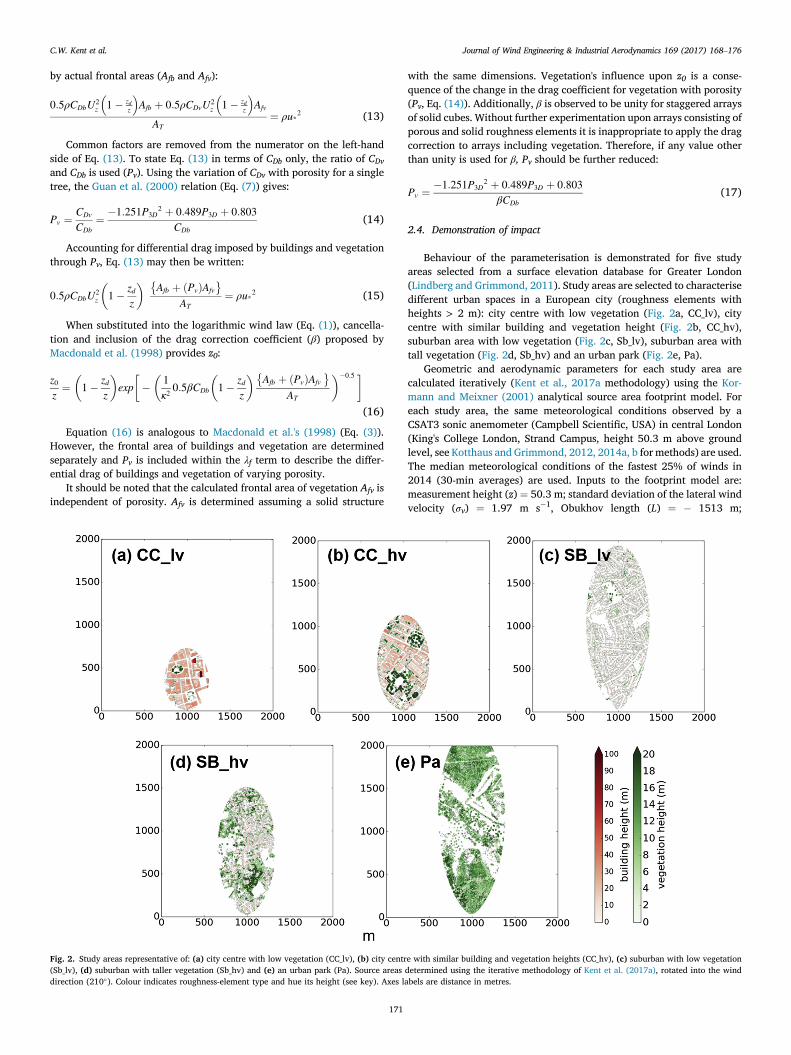
Fig. 2. Study areas representative of: (a) city centre with low vegetation (CC_lv), (b) city centr(Sb_lv), (d) suburban with taller vegetation (Sb_hv) and (e) an urban park (Pa). Source areasdirection (210�). Colour indicates roughness-element type and hue its height (see key). Axes la

171

with the same dimensions. Vegetation's influence upon z0 is a conse-quence of the change in the drag coefficient for vegetation with porosity(Pv, Eq. (14)). Additionally, β is observed to be unity for staggered arraysof solid cubes. Without further experimentation upon arrays consisting ofporous and solid roughness elements it is inappropriate to apply the dragcorrection to arrays including vegetation. Therefore, if any value otherthan unity is used for β, Pv should be further reduced:

Pv ¼ �1:251P3D2 þ 0:489P3D þ 0:803

βCDb(17)

2.4. Demonstration of impact

Behaviour of the parameterisation is demonstrated for five studyareas selected from a surface elevation database for Greater London(Lindberg and Grimmond, 2011). Study areas are selected to characterisedifferent urban spaces in a European city (roughness elements withheights > 2 m): city centre with low vegetation (Fig. 2a, CC_lv), citycentre with similar building and vegetation height (Fig. 2b, CC_hv),suburban area with low vegetation (Fig. 2c, Sb_lv), suburban area withtall vegetation (Fig. 2d, Sb_hv) and an urban park (Fig. 2e, Pa).

Geometric and aerodynamic parameters for each study area arecalculated iteratively (Kent et al., 2017a methodology) using the Kor-mann and Meixner (2001) analytical source area footprint model. Foreach study area, the same meteorological conditions observed by aCSAT3 sonic anemometer (Campbell Scientific, USA) in central London(King's College London, Strand Campus, height 50.3 m above groundlevel, see Kotthaus and Grimmond, 2012, 2014a, b for methods) are used.The median meteorological conditions of the fastest 25% of winds in2014 (30-min averages) are used. Inputs to the footprint model are:measurement height (z) ¼ 50.3 m; standard deviation of the lateral windvelocity (σv) ¼ 1.97 m s�1, Obukhov length (L) ¼ � 1513 m;

e with similar building and vegetation heights (CC_hv), (c) suburban with low vegetationdetermined using the iterative methodology of Kent et al. (2017a), rotated into the windbels are distance in metres.

Table 1Geometric parameters determined for: all roughness elements; vegetation only; and buildings only, in the five study areas (Fig. 2). Hav, Hmax and σH are the average, maximum and standarddeviation of roughness-element heights (in metres), respectively, λp is plan area index and λf is frontal area index. Subscripts: v for vegetation, b for buildings, l-on for leaf-on and l-off for leaf-off.

Area All Vegetation Buildings

Hav Hmax σH λp,l-on λp,l-off λf,l-ona λf,l-off

a Hav,v Hmax,v σH,v λp,v,l-on λp,v, l-off λf,v Hav,b Hmax,b σH,b λp,b λf,b

CC_lv 23.50 125.00 15.00 0.54 0.52 0.52 0.51 10.90 35.00 8.78 0.03 0.01 0.04 24.50 125.00 15.00 0.51 0.49CC_hv 14.90 46.60 7.99 0.48 0.37 0.42 0.37 15.70 34.00 7.47 0.21 0.11 0.26 14.10 46.60 8.22 0.27 0.23SB_lv 5.34 27.80 2.64 0.29 0.25 0.18 0.17 4.82 27.80 3.46 0.08 0.04 0.08 5.58 16.60 2.00 0.21 0.13SB_hv 10.80 33.30 5.37 0.47 0.33 0.33 0.28 11.60 33.30 5.78 0.29 0.14 0.29 9.12 28.10 3.75 0.18 0.12Pa 11.30 29.00 4.67 0.60 0.30 0.29 0.22 11.40 29.00 4.63 0.59 0.30 0.41 5.75 16.50 2.39 0.00 0.00

a λf,l-on and λf,l-off ¼�fAfbþðPv ÞAfvg

AT

�, assuming a leaf-on and leaf-off porosity, respectively.

C.W. Kent et al. Journal of Wind Engineering & Industrial Aerodynamics 169 (2017) 168–176

u* ¼ 0.94 m s�1; wind direction 210�; zd and z0. Source area calculationsare initiated with open country values for the aerodynamic parameters(zd ¼ 0.2 m, z0 ¼ 0.03 m), as the final values are insensitive to this initialassumption (Kent et al., 2017a). The source area analysed here is thecumulative total of 80% of the total source area.

Dynamic response of the source areas during the iterative proceduremodifies the surface area considered. The initial source area is overlainupon the surface elevation databases (buildings and vegetation) for eachstudy area and a weighted geometry is calculated, based upon the frac-tional contribution of each grid square in the source area. Source areaspecific aerodynamic parameters are determined, which are the input tothe next iteration (the meteorological conditions and measurementheight remain constant). Both buildings and vegetation are considered,assuming a leaf-on porosity of P3D¼ 0.2, and leaf-off porosity of P3D¼ 0.6(more porous) (Heisler, 1984; Heisler and Dewalle, 1988; Grimmond andOke, 1999).

Variations in meteorological conditions between sites probably occur,however the objective to obtain representative study areas (Fig. 2a–e,Table 1) means the assumption of constant conditions is treated asreasonable. The resulting geometry and (Mac and Kan) aerodynamicparameters are compared for each study area (Sect. 3.1 and 3.2).

Using the logarithmic wind law (Eq. (1)) the implications of consid-ering vegetation during wind-speed estimation close to the surface arethen assessed (Sect. 3.3). Using the zd and z0 determined for buildingsonly, or both buildings and vegetation, for the five study areas, windspeeds are extrapolated from zd þ z0 to 100 m using Eq. (1). For con-sistency, at zdþ z0 it is assumed the wind speed is 0 m s�1 and throughoutthe profile the previously stated central London friction velocity(u* ¼ 0.94 m s�1) is assumed. Although choosing a different value of u*will have implications for the estimated wind speeds, the relativemagnitude of change for each profile is the same and therefore so are thepercentage differences between profiles. The objective is to demonstratethe implications of considering (or not) vegetation for each morpho-metric method and study area, as opposed to providing a comparisonbetween the study areas.

Table 2Aerodynamic parameters determined using the Macdonald et al. (1998,Mac) and Kanda et al. (20for buildings only and for all roughness elements (both buildings and vegetation), with leaf-on

172

3. Results

3.1. Geometric parameters

Obviously, the influence of vegetation and buildings upon geometricparameters depends upon the dominant roughness elements: whenbuildings dominate (CC_lv and CC_hv), height based geometric parame-ters for all roughness elements (both buildings and vegetation) aredetermined by buildings (Table 1); and, if vegetation is taller thanbuildings (SB_hv and Pa), the Hav, Hmax and σH of all roughness elementsbecome noticeably larger than Hav,b, Hmax,b and σH,b (Table 1, subscript bdenotes buildings only). In all study areas, the effect of vegetation in-creases both plan and frontal areas, which is expectedly more obvious forleaf-on than leaf-off values. In CC_lv the plan and frontal area indexes ofvegetation (λp,v and λf,v) are effectively negligible. Elsewhere the tallerand higher proportion of vegetation means λp,v and λf,v are greater than orsimilar to that of buildings (λp,b and λf,b). This means plan and frontalareas calculated for all roughness elements can be double or larger thanthat for buildings alone (Table 1, SB_hv and CC_hv).

Leaf state has a greater impact upon plan than frontal area, with meandifferences of 0.12 (λp,l-on – λp,l-off) and 0.04 (λf,l-on and λf,l-off), respectively,across the five study areas (subscripts l-on and l-off refer to leaf-on or offvegetation state, respectively). As this difference is proportional to theamount of vegetation present, it is maximum in Pa where leaf-on planarea index is approximately double leaf-off (0.6 and 0.3, respectively).

Implications of ignoring vegetation (i.e. only considering buildings)are most obvious in Pa. Here the plan and frontal area of buildingsapproach 0, whilst λf,v is 0.41 and λp,v ranges between 0.3 and 0.59 forleaf-off and leaf-on porosity, respectively (Table 1). The average height ofbuildings is only 5.8 m with a maximum of 16.5 m. However, the averageheight of vegetation (Hav,v) is almost as large as the tallest building(11.4 m) and maximum tree height (Hmax,v) is 29 m. Therefore, the ge-ometry in Pa is primarily determined by the vegetation characteris-tics (Table 1).

13, Kan) morphometric methods in the five study areas (Fig. 2). Parameters are determined(l-on) and leaf-off (l-off) vegetation.

Table 3Percentage difference in aerodynamic parameters calculated using the (a) Macdonald et al. (1998) and (b) Kanda et al. (2013) morphometric methods from Table 2, between: buildings (x)and all roughness elements (y) assuming a leaf-on porosity (b, l-on); buildings (x) and all roughness elements (y) assuming a leaf-off porosity (b, l-off) and for all roughness elements assuminga leaf-on (x) or leaf-off porosity (y) (l-on, l-off). Percentage difference ¼ jx�yj

ðxþyÞ=2 � 100.

Table 4Percentage difference in aerodynamic parameters calculated using the Macdonald et al. (1998, Mac) (x) or Kanda et al. (2013, Kan) (y) morphometric methods from Table 2, for buildingsonly and all roughness elements assuming a leaf-on porosity (l-on) and leaf-off porosity (l-off). Percentage difference ¼ jx�yj

ðxþyÞ=2 � 100.

C.W. Kent et al. Journal of Wind Engineering & Industrial Aerodynamics 169 (2017) 168–176

3.2. Aerodynamic parameters

For aerodynamic parameter determination, the geometric parameters

Fig. 3. Logarithmic wind-speed profiles (using Eq. (1)) from z ¼ zd þ z0 to z ¼ 100 m, using zdcentre with similar building and vegetation heights (CC_hv), (c) a suburb with low vegetationbottom of the profile (zd þ z0) is assumed 0 m s�1 and friction velocity (u*) 0.94 m s�1 througdetermined are using the Kanda et al. (2013) (Kan) and Macdonald et al. (1998) (Mac) morpvegetation with leaf-off porosity (short dashed line) and leaf-on porosity (long dashed line) (v

173

within the morphometric methods (e.g. Kan considers height variability)are important, in addition to the dominance of either buildings orvegetation. For a heterogeneous group of roughness elements Kanzd is

and z0 determined for five study areas: (a) city centre with low vegetation (CC_lv), (b) city(Sb_lv), (d) a suburb with taller vegetation (Sb_hv) and (e) a park (Pa). Wind speed at thehout the profile. Wind speeds are normalised by u* (Uz/u*). Aerodynamic parameters arehometric methods for each study area, considering buildings only (solid line), includingalues in Table 2). Note different x scale on (e).

C.W. Kent et al. Journal of Wind Engineering & Industrial Aerodynamics 169 (2017) 168–176

typically twice as large as Maczd at all densities. Macz0 is observed to belarger than Kanz0 at λf below ~0.25, beyond which Kanz0 is larger (Kentet al., 2017a; their Fig. 1).

Generally, accounting for vegetation (with buildings) increases zdbecause the increase in plan area acts to ‘close’ the canopy and thereforelift the zero-plane displacement (Table 2). The effect is most obviousduring leaf-on and where there is a higher density of vegetation (SB_hv,Pa). This creates a greater than 40% difference between zd calculated forbuildings alone and the combined case (buildings and vegetation). CC_lvis the only area where considering vegetation may reduce zd because asmall increase in λp is offset by a reduction in Hav (Table 2). Leaf-on zd isalways greater than leaf-off, but the difference is less obvious for the Kanmethod as height variability (in addition to λp) is accounted for.

Kanzd is consistently the order of Hav (or larger) and typically overdouble Maczd (Table 2). The range of percentage change for zd caused byvegetation inclusion and its state (Table 3) tend to be over half the inter-method variability of Kanzd and Maczd (Table 4). Thus, the priority ofdecisions for accurate determination of zd is firstly selection of theappropriate morphometric method, followed by the inclusion of vege-tation and then its state (leaf-on or leaf-off). An exception is in Pa, wherevegetation has the largest effect.

The effect of considering vegetation for z0 depends upon: the heightbased geometric parameters, the increase in λf and λp; and the associatedchange in zd. The inter- and intra-method differences of Mac and Kandepend upon their response to changes in λf. Both methods indicate z0increases from zero to a maximum value at a critical λf (λf-crit), after whichz0 decreases again. For Macz0 , λf-crit is between ~0.15–0.25 and for Kanz0this is 0.2–0.4 (Kent et al., 2017a; their Fig. 1). At larger λf, there is asteeper decline in Macz0 than Kanz0 .

When an already large built frontal area is further increased due tothe vegetation (CC_lv, CC_hv), leaf-on z0 becomes smaller for bothmethods as there is a shift further away from λf-crit. For both CC_lv andCC_hv the percentage changes are larger for Macz0 than Kanz0 given thesensitivity of the former to changes of λf. The reduction is greater for leaf-on because of the larger λf (Table 1).

In locations with low built frontal areas (Table 1, SB_hv, SB_lv) theinclusion of vegetation should increaseMacz0 and Kanz0 given they movetowards λf-crit. This is true for Kanz0 , most obviously in SB_hv (17% dif-ference for leaf-on and 47% for leaf-off, Table 3) where vegetation ismore dominant and Hmax, σH and λp become obviously larger. However,for Macz0 , the λf increase is offset by the concurrent increase in zd(Table 2). ThereforeMacz0 decreases for leaf-on conditions, but is similarfor leaf-off. For Pa, inclusion of vegetationmeansMacz0 ;b and Kanz0 ;b bothincrease from 0 m to 0.18 and 0.32 m, respectively during leaf-on, and to0.99 and 0.92 m, respectively for leaf-off (Table 2). If only buildings areconsidered, the variability between Kanz0 ;b andMacz0 ;b is less than 35% inall study areas apart from CC_lv, where Kanz0 ;b is more than doubleMacz0 ;b because of the large λf,b (~0.5).

Leaf-on z0 is consistently smaller than leaf-off for both morphometricmethods as a consequence of both λf and zd increasing. The greatersensitivity ofMacz0 to λf results in a percent difference that is twice that ofKanz0 , except in Pa where both experience large increases (Table 3).During leaf-off, areas with λf similar to λf-crit (e.g. SB_lv, SB_hv) have meaninter-method variability of < ~10%. Whereas if there are already high λf(SB_hv, CC_hv and CC_lv), an increase in λf with leaf-on vegetation causesinter-method variability to increase, ranging between 48 and95% (Table 4).

Therefore, if buildings dominate (e.g. CC_hv) selection of theappropriate morphometric method is more critical for determining z0(causing a larger percentage difference in z0) than if vegetation isincluded. The inclusion of vegetation increases inter-method variabilitybetween the two morphometric methods (e.g. CC_hv and CC_lv). Wherethere is more vegetation, its inclusion and state (leaf-on or off), is as ormore important than the inter-method variability in z0. This is especiallytrue for Pa.

174

3.3. Influence of considering vegetation upon wind

Accurately modelling the spatially- and temporally-averaged wind-speed profile above urban surfaces is critical for numerous applications,including dispersion studies and wind load determination. Variousmethods to estimate the wind-speed profile exist, each developed fromdifferent conditions and with different inherent assumptions (e.g. Deavesand Harris, 1978; Emeis et al., 2007; Gryning et al., 2007). However, theaerodynamic roughness parameters (zd and z0) are consistently used torepresent the underlying surface. Although only two methods to deter-mine the roughness parameters are used here (Mac and Kan), a range ofmethods exist which can influence wind-speed estimations (Kentet al., 2017a).

Using the logarithmic wind law (Eq. (1)), wind-speeds extrapolatedusing the Kan method tend to be less than those using Mac (Fig. 3a–e)because of the considerably larger Kanzd . Notably, where zd is largest inmagnitude (e.g. CC_lv, Table 2) wind speeds at 100 m calculated usingthe Kan or Mac aerodynamic parameters vary between 36 and 39% ofeach other (depending on vegetation state). Elsewhere, extrapolatedwind speeds tend to be more similar, and the least variable aerodynamicparameters in SB_lv and SB_hv mean wind speeds at 100 m vary by lessthan 4% and 12%, respectively.

The difference in wind speed when both buildings and vegetation areaccounted for (Fig. 3, dashed lines), in comparison to buildings alone(Fig. 3, solid lines) is least where buildings dominate. For example, inCC_lv and SB_lv vegetation has little effect and regardless of its statecauses a maximum wind-speed variation of <5% for each respectivemorphometric method.

Consideration of vegetation in the morphometric methods has agreater influence upon predicted wind speeds where vegetation is tallerand more abundant (e.g. CC_hv, SB_hv and Pa). In addition, vegetationstate (i.e. leaf-on or leaf-off) is more influential upon wind speeds in theseareas. Despite zd increasing with inclusion of vegetation, there is greaterinter- and intra-method variability in z0 (Sect. 3.2). Therefore, becauseestimated wind profiles are a function of both zd and z0 no generalcomment can be made about wind-speed changes when includingvegetation.

Vegetation's effect is most noticeable in Pa. High wind speeds whenonly buildings are considered (because of low zd and z0) are reduced byalmost a factor of three upon consideration of vegetation (Fig. 3e). Thereduction in wind speed is more obvious for leaf-off porosities, because ofthe larger associated z0. In CC_hv and SB_hv the effect of vegetation is lessobvious, however a decrease in z0 means wind speeds extrapolated usingtheMac parameters increase. In contrast, wind speeds extrapolated usingthe Kan parameters tend to decrease because of the larger zd and lessersensitivity to changes in z0 (Sect. 3.2).

In summary, when buildings dominate (CC_lv) the morphometricmethod chosen to determine the wind profile (i.e. Mac or Kan) is moreimportant than whether vegetation is considered. In contrast, wherevegetation is taller and accounts for a greater surface area (CC_hv, SB_hvand especially Pa) vegetation's consideration has larger implications forwind-speed estimation than the morphometric method used. In all cases,the differences between leaf-on and leaf-off wind speed are larger for theMac than Kan method, because of the sensitivity of Mac to the porosityparameterisation.

4. Conclusions

Vegetation should be included in morphometric determination ofaerodynamic parameters, but not in the same way as solid structures. Amethodology is proposed to include vegetation in Macdonald et al.'s(1998) morphometric method to determine the zero-plane displacement(zd) and aerodynamic roughness length (z0). This also applies to Kandaet al.'s (2013) extension, which considers roughness-element heightvariability.

The proposed methodology considers the average, maximum and

C.W. Kent et al. Journal of Wind Engineering & Industrial Aerodynamics 169 (2017) 168–176

standard deviation of heights for all roughness elements (buildings andvegetation). The plan area index and frontal area index of buildings andvegetation are determined separately (and subsequently combined foruse in the morphometric methods). Aerodynamic porosity is used todetermine the plan area of vegetation. Whereas, the frontal area index ofvegetation is determined assuming a solid structure with the same di-mensions. During determination of z0 a parameterisation of the dragcoefficient for vegetation is used, accounting for varying porosity. Thisfollows literature that demonstrates the drag exerted by trees can be likethat of a solid structure and decreases as porosity increases (Grant andNickling, 1998; Guan et al., 2000; Vollsinger et al., 2005; Koizumi et al.,2010). The relation between the drag coefficient and porosity of an in-dividual tree (Guan et al., 2000) is used as the basis for the parameter-isation, which other experimental data demonstrate is reasonable.

From analysis of five different urban areas within a European city, theeffect of the inclusion of vegetation on geometric and aerodynamic pa-rameters depends upon whether buildings or vegetation are the domi-nant roughness element. Where buildings are taller they control theheight-based geometric parameters. The opposite is true when vegeta-tion is taller. Inclusion of vegetation increases the plan area index (λp)and frontal area index (λf), most obviously during leaf-on periods.

The increases in λp and λf from inclusion of vegetation more obviouslyaffect aerodynamic parameters than the change in height based geo-metric parameters. The higher λp produces a larger zd for both morpho-metric methods in four study areas. In the fifth case, a reduction inaverage height offsets the increase in λp. The increase in zd is largest forleaf-on because of the higher λp, as well as where vegetation is taller andmore significant because of the greater increase in λp and average height(Hav). Given the large inter-method variability in zd, selection of theappropriate morphometric method is most critical, followed by whethervegetation is considered, then by the vegetation state (leaf-on or leaf-off).

Inclusion of the effect of vegetation on z0 depends upon: the geo-metric parameters determined without vegetation and the associated λfthat the peak z0 occurs for each morphometric method. Therefore, abroad statement about how z0 responds to vegetation inclusion is diffi-cult. However, the change in z0 is more obvious where vegetation is tallerand takes up a large proportion of area. In the same areas, whethervegetation is included and its state (i.e. porosity) is as, or more important,than the inter-method variability in z0 determined by the morphometricmethods. Leaf-on z0 is consistently smaller than leaf-off, because of thecombined increase in λf and zd which create an effectivelysmoother surface.

Assuming a logarithmic wind profile, the influence on estimated windspeed up to 100 m is least when vegetation is lower and accounts for asmaller proportion of surface area, with wind speed varying by < 5%regardless of consideration of vegetation. In contrast, wind speeds abovean urban park are demonstrated to be slowed by up to a factor of three(both methods). Therefore, if vegetation is taller and more abundant,vegetation's inclusion is as, or more, critical for wind-speed estimationthan the morphometric method used.

Of course, the ultimate assessment of the parameterisation for accu-rate aerodynamic parameter and wind-speed estimation is comparison toobservations. An assessment of the parameterisation, demonstrates theseasonal change in aerodynamic parameters can be captured and wind-speed estimations improved (Kent et al. 2017b). Undoubtedly, furtherobservations and wind tunnel experiments with various arrays of solidand porous roughness elements will be valuable to assess theparameterisation.

Funding

This work is funded by a NERC CASE studentship in partnership withRisk Management Solutions (NE/L00853X/1) and the Newton Fund/MetOffice CSSP China. Observations used in these analyses are funded fromNERC ClearfLo (KCL and Reading), EUf7 BRIDGE, EUf7 emBRACE,H2020 UrbanFluxes, EPSRC BTG, KCL and University of Reading.

175

Acknowledgements

The numerous people who maintain the daily operations, collectionand processing of data for the London Urban Meteorological Observatory(LUMO) network (http://micromet.reading.ac.uk/), including WillMorrison and Kjell zum Berge. King's College London support for provi-sion of the sites. The morphometric method development (includingvegetation) and source area calculation are implemented into the UrbanMulti-scale Environmental Predictor (UMEP, http://www.urban-climate.net/umep/UMEP) climate service plugin for the open source soft-ware QGIS.

References

Amiro, B., 1990. Drag coefficients and turbulence spectra within three boreal forestcanopies. Boundary-Laye Meteorol. 52, 227–246.

Bitog, J., Lee, I., Hwang, H., Shin, M., Hong, S., Seo, I., Mostafa, E., Pang, Z., 2011. A windtunnel study on aerodynamic porosity and windbreak drag. For. Sci. Technol. 7,8–16.

Cheng, H., Hayden, P., Robins, A.G., Castro, I.P., 2007. Flow over cube arrays of differentpacking densities. J. Wind Eng. Ind. Aerodyn. 95, 715–740.

Crow, P., Benham, S., Devereux, B., Amable, G., 2007. Woodland vegetation and itsimplications for archaeological survey using LiDAR. Forestry 80, 241–252.

da Costa, J.L., Castro, F., Palma, J., Stuart, P., 2006. Computer simulation of atmosphericflows over real forests for wind energy resource evaluation. J. Wind Eng. Ind.Aerodyn. 94, 603–620.

Deaves, D., Harris, R., 1978. A Mathematical Model of the Structure of Strong Winds.Report number 76. Construction Industry Research and Information Association,London, England.

Drew, D.R., Barlow, J.F., Lane, S.E., 2013. Observations of wind speed profiles overGreater London, UK, using a Doppler lidar. J. Wind Eng. Ind. Aerodyn. 121, 98–105.

Emeis, S., Baumann-Stanzer, K., Piringer, M., Kallistratova, M., Kouznetsov, R.,Yushkov, V., 2007. Wind and turbulence in the urban boundary layer–analysis fromacoustic remote sensing data and fit to analytical relations. Meteorol. Z. 16, 393–406.

Finnigan, J., 2000. Turbulence in plant canopies. Annu. Rev. Fluid Mech. 32, 519–571.Gillies, J., Lancaster, N., Nickling, W., Crawley, D., 2000. Field determination of drag

forces and shear stress partitioning effects for a desert shrub (Sarcobatusvermiculatus, greasewood). J. Geophys Res. D. Atmos. 105, 24871–24880.

Gillies, J., Nickling, W., King, J., 2002. Drag coefficient and plant form response to windspeed in three plant species: burning Bush (Euonymus alatus), Colorado Blue Spruce(Picea pungens glauca.), and Fountain Grass (Pennisetum setaceum). J. Geophys Res.D. Atmos. 107, 4760.

Grant, P., Nickling, W., 1998. Direct field measurement of wind drag on vegetation forapplication to windbreak design and modelling. Land Degrad. Dev. 9, 57–66.

Grimmond, C.S.B., Oke, T.R., 1999. Aerodynamic properties of urban areas derived fromanalysis of surface form. J Appl Meteorol Clim 38, 1262–1292.

Gromke, C., Ruck, B., 2009. On the impact of trees on dispersion processes of trafficemissions in street canyons. Boundary-Layer Meteorol. 131, 19–34.

Gryning, S., Batchvarova, E., Brümmer, B., Jørgensen, H., Larsen, S., 2007. On theextension of the wind profile over homogeneous terrain beyond the surface boundarylayer. Boundary-Layer Meteorol. 124, 251–268.

Guan, D., Ting-Yao, Z., Shi-Jie, H., 2000. Wind tunnel experiment of drag of isolated treemodels in surface boundary layer. J. For. Res. 11, 156–160.

Guan, D., Zhang, Y., Zhu, T., 2003. A wind-tunnel study of windbreak drag. Agric ForMeteorol 118, 75–84.

Guan, W., Li, C., Li, S., Fan, Z., Xie, C., 2002. Improvement and application of digitizedmeasure on shelterbelt porosity. J. Appl. Ecol. 13, 651–657.

Hagen, L., Skidmore, E., 1971. Windbreak drag as influenced by porosity. Trans. ASAE 14,464–0465.

Hall, D., Macdonald, J.R., Walker, S., Spanton, A.M., 1996. Measurements of Dispersionwithin Simulated Urban Arrays—a Small Scale Wind Tunnel Study. BRE ClientReport, CR178/96.

Heisler, G.M., 1984. Measurements of solar radiation in the shade of individual trees. In:Hutchinson, B.A., Hicks, B.B. (Eds.), The Forest-Atmosphere Interaction. Springer,Netherlands, pp. 319–355.

Heisler, G.M., Dewalle, D.R., 1988. Effects of windbreak structure on wind flow. Agric.Ecosyst. Environ. 22, 41–69.

H€ogstr€om, U., 1996. Review of some basic characteristics of the atmospheric surfacelayer. Boundary-Layer Meteorol. 28, 215–246.

Holland, D.E., Berglund, J.A., Spruce, J.P., McKellip, R.D., 2008. Derivation of effectiveaerodynamic surface roughness in urban areas from airborne lidar terrain data.J Appl Meteorol Clim 47, 2614–2626.

Jacobs, A.F., 1985. The normal-force coefficient of a thin closed fence. Boundary-LayerMeteorol. 32, 329–335.

Judd, M., Raupach, M., Finnigan, J., 1996. A wind tunnel study of turbulent flow aroundsingle and multiple windbreaks, part I: velocity fields. Boundary-Layer Meteorol. 80,127–165.

Kanda, M., Inagaki, A., Miyamoto, T., Gryschka, M., Raasch, S., 2013. A new aerodynamicparametrization for real urban surfaces. Boundary-Layer Meteorol. 148, 357–377.

Katul, G.G., Mahrt, L., Poggi, D., Sanz, C., 2004. One-and two-equation models for canopyturbulence. Boundary-Layer Meteorol. 113, 81–109.

C.W. Kent et al. Journal of Wind Engineering & Industrial Aerodynamics 169 (2017) 168–176

Kent, C.W., Grimmond, C.S.B., Gatey, D., Barlow, J., Kotthaus, S., Lindberg, F.,Halios, C.H., 2017. Evaluation of urban local-scale aerodynamic parameters:implications for the vertical profile of wind speed and for source areas. Boundary-Layer Meteorol. http://dx.doi.org/10.1007/s10546-017-0248-z.

Kent, C.W., Lee, K., Ward, H.C., Hong, J.W., Hong, J., Grimmond, C.S.B., 2017.Aerodynamic roughness variation with vegetation: analysis in a suburbanneighbourhood and a city park (in review).

Koizumi, A., Motoyama, J., Sawata, K., Sasaki, Y., Hirai, T., 2010. Evaluation of dragcoefficients of poplar-tree crowns by a field test method. J. Wood Sci. 56, 189–193.

Kormann, R., Meixner, F.X., 2001. An analytical footprint model for non-neutralstratification. Boundary-Layer Meteorol. 99, 207–224.

Kotthaus, S., Grimmond, C.S.B., 2012. Identification of micro-scale anthropogenic CO2,heat and moisture sources–processing eddy covariance fluxes for a dense urbanenvironment. Atmos. Environ. 57, 301–316.

Kotthaus, S., Grimmond, C.S.B., 2014a. Energy exchange in a dense urbanenvironment–Part I: temporal variability of long-term observations in central London.Urban Clim. 10, 261–280.

Kotthaus, S., Grimmond, C.S.B., 2014b. Energy exchange in a dense urbanenvironment–Part II: impact of spatial heterogeneity of the surface. Urban Clim. 10,281–307.

Krayenhoff, E., Santiago, J., Martilli, A., Christen, A., Oke, T., 2015. Parametrization ofdrag and turbulence for urban neighbourhoods with trees. Boundary-Layer Meteorol.156, 157–189.

Lindberg, F., Grimmond, C.S.B., 2011. Nature of vegetation and building morphologycharacteristics across a city: influence on shadow patterns and mean radianttemperatures in London. Urban Ecosyst. 14, 617–634.

Macdonald, R., Griffiths, R., Hall, D., 1998. An improved method for the estimation ofsurface roughness of obstacle arrays. Atmos. Environ. 32, 1857–1864.

Mayhead, G., 1973. Some drag coefficients for British forest trees derived from windtunnel studies. Agric. Meteorol. 12, 123–130.

Millward-Hopkins, J., Tomlin, A., Ma, L., Ingham, D., Pourkashanian, M., 2011.Estimating aerodynamic parameters of urban-like surfaces with heterogeneousbuilding heights. Boundary-Layer Meteorol. 141, 443–465.

Mohammad, A., Zaki, S., Hagishima, A., Ali, M., 2015. Determination of aerodynamicparameters of urban surfaces: methods and results revisited. Theor. Appl. Climatol. 3,635–649.

Nakai, T., Sumida, A., Daikoku, K.I., Matsumoto, K., van der Molen, M.K., Kodama, Y.,Kononov, A.V., Maximov, T.C., Dolman, A.J., Yabuki, H., Hara, T., 2008.Parameterisation of aerodynamic roughness over boreal, cool-and warm-temperateforests. Agric. For. Meteorology 148, 1916–1925.

Pan, Y., Follett, E., Chamecki, M., Nepf, H., 2014. Strong and weak, unsteadyreconfiguration and its impact on turbulence structure within plant canopies. Phys.Fluids 26, 105102.

176

Rudnicki, M., Mitchell, S.J., Novak, M.D., 2004. Wind tunnel measurements of crownstreamlining and drag relationships for three conifer species. Can. J. For. Res. 34,666–676.

Seginer, I., 1975. Atmospheric-stability effect on windbreak shelter and drag. Boundary-Layer Meteorol. 8, 383–400.

Shaw, R.H., Patton, E.G., 2003. Canopy element influences on resolved-and subgrid-scaleenergy within a large-eddy simulation. Agric For Meteorol 115, 5–17.

Shaw, R.H., Schumann, U., 1992. Large-eddy simulation of turbulent flow above andwithin a forest. Boundary-Layer Meteorol. 61, 47–64.

Simiu, E., Scanlan, R.H., 1996. Wind Effects on Structures. Wiley, New York, p. 605.Su, H., Shaw, R.H., Paw, K.T., Moeng, C., Sullivan, P.P., 1998. Turbulent statistics of

neutrally stratified flow within and above a sparse forest from large-eddy simulationand field observations. Boundary-Layer Meteorol. 88, 363–397.

Suter-Burri, K., Gromke, C., Leonard, K.C., Graf, F., 2013. Spatial patterns of aeoliansediment deposition in vegetation canopies: observations from wind tunnelexperiments using colored sand. Aeolian Res. 8, 65–73.

Sutton, S., McKenna Neuman, C., 2008. Sediment entrainment to the lee of roughnesselements: effects of vortical structures. J. Geophys. Res. Earth Surf. 113. F02S09.

Taylor, P.A., 1988. Turbulent wakes in the atmospheric boundary layer. In: Steffen, W.L.,Denmead, O.T. (Eds.), Flow and Transport in the Natural Environment: Advances andApplications. Springer, Berlin, pp. 270–292.

Tennekes, H., 1973. The logarithmic wind profile. J. Atmos. Sci. 30, 234–238.Tieleman, H.W., 2008. Strong wind observations in the atmospheric surface layer.

J. Wind Eng. Ind. Aerodyn. 96, 41–77.Van Renterghem, T., Botteldooren, D., 2008. Numerical evaluation of sound propagating

over green roofs. J. Sound. Vibrat 317, 781–799.Vollsinger, S., Mitchell, S.J., Byrne, K.E., Novak, M.D., Rudnicki, M., 2005. Wind tunnel

measurements of crown streamlining and drag relationships for several hardwoodspecies. Can. J. For. Res. 35, 1238–1249.

Vos, P.E., Maiheu, B., Vankerkom, J., Janssen, S., 2013. Improving local air quality incities: to tree or not to tree? Environ. Pollut. 183, 113–122.

Wilson, J.D., 1985. Numerical studies of flow through a windbreak. J. Wind Eng. Ind.Aerodyn. 21, 119–154.

Wolfe, S.A., Nickling, W.G., 1993. The protective role of sparse vegetation in winderosion. Prog. Phys. Geogr. 17, 50–50.

Wyatt, V., Nickiing, W., 1997. Drag and shear stress partitioning in sparse desert creosotecommunities. Can. J. Earth Sci. 34, 1486–1498.

Yang, X., Yu, Y., Fan, W.A., 2017. A method to estimate the structural parameters ofwindbreaks using remote sensing. Agrofor. Syst. 91, 37–49.

Zeng, P., Takahashi, H., 2000. A first-order closure model for the wind flow within andabove vegetation canopies. Agric For Meteorol 103, 301–313.