JOURNAL OF UNDERGRADUATE RESEARCH · Journal of Undergraduate Research ... the CO-Synch protocol...
84
South Dakota State University JOURNAL OF UNDERGRADUATE RESEARCH Volume 8 • 2010
Transcript of JOURNAL OF UNDERGRADUATE RESEARCH · Journal of Undergraduate Research ... the CO-Synch protocol...

South Dakota State University
JOURNAL OFUNDERGRADUATE
RESEARCH
Volume 8 • 2010
GS019 JUR10_GS JUR text 1/11/11 11:41 AM Page 1

The South Dakota State UniversityJournal of Undergraduate Research
is published annually by the Office of Research & Sponsored Programs at South Dakota State University
EditorDr. George Langelett
Associate EditorLinda Winkler
All assertions of fact or statements of opinion are solely those of the authors. They do not necessarily represent the views of the
Editorial Board, the Office of Research & Sponsored Programs, South Dakota State University or its faculty and administration.
All correspondence, including requests for copies of the Journal, should be sent to:
South Dakota State UniversityJournal of Undergraduate Research
Office of Research & Sponsored Programs130 Administration Building
Brookings, SD 57007
GS019 JUR10_GS JUR text 1/11/11 11:41 AM Page 2

South Dakota State University
JOURNAL OFUNDERGRADUATE
RESEARCH
Volume 8 • 2010
GS019 JUR10_GS JUR text 1/11/11 11:41 AM Page i

Table of Contents
Guidelines – SDSU Journal of Undergraduate Research . . . . . . . . . . . . . . iv
Effect of Standing Estrus Prior to n Injectio of GnRH on
Steriodogenic Enzyme Expression in Luteal Tissue
KAYCEE GEBHART . . . . . . . . . . . . . . . . . . . . . . . . . . . . . . . . . . . . . . . . . . . . 1
Affect Comprehension in Children With Autism Spectrum
Disorder: A Visual Field Isolation Intervention
ERICA L. SCHMIDT. . . . . . . . . . . . . . . . . . . . . . . . . . . . . . . . . . . . . . . . . . . 11
Parental Influence on the Financial Literacy of Their School-Aged
Children: An Exploratory Study
STEPHANIE WILLIAMS . . . . . . . . . . . . . . . . . . . . . . . . . . . . . . . . . . . . . . . . 23
Formula SAE Impact Attenuator Testing
CHAD ABRAHAMSON, BILL BRUNS, JOSEPH HAMMOND, JOSH LUTTER . . . . . . .35
Serial and Concurrent Presentations of Stimuli and Their Effects
on Items Recalled
DUSTIN J. RHOADES, JORDAN SIPPEL . . . . . . . . . . . . . . . . . . . . . . . . . . . . . . 47
The Effects of Feedback on Student Performance While Performing
Multiple Tasks Simultaneously
AMBER REIS, DANYEL JANSSEN . . . . . . . . . . . . . . . . . . . . . . . . . . . . . . . . . 57
Tracking Bare Sand Mobilization Arising From Landscape
Manipulations in the Grasslands Destabilization Experiment
(GDEX) in the Nebraska Sandhills Using Imaging Spectroscopy
BENJAMIN HELDER, B.S.. . . . . . . . . . . . . . . . . . . . . . . . . . . . . . . . . . . . . . . 65
Working Mothers: Cognitive and Behavioral Effects on Children
AMANDA DEJONG . . . . . . . . . . . . . . . . . . . . . . . . . . . . . . . . . . . . . . . . . . . 75
iii
GS019 JUR10_GS JUR text 1/11/11 11:41 AM Page iii

The Journal of Undergraduate Research would like to thank
Dr. Kevin Kephart, Vice President for Research, for his efforts
to secure funding for the Journal.
GS019 JUR10_GS JUR text 1/11/11 11:41 AM Page x

EFFECT OF STANDING ESTRUS PRIOR TO AN INJECTION OF GnRH 1
Effect of Standing Estrus Prior to anInjection of GnRH on SteriodogenicEnzyme Expression in Luteal Tissue
Author: Kaycee GebhartFaculty Sponsor: Dr. George PerryDepartment: Animal Science
ABSTRACTCows detected in estrus around the time of fixed-time AI had increased pregnancy
success and progesterone concentrations. Additionally, GnRH following onset of estrus
influenced LH pulse frequency and CL formation/function. Therefore our objective was to
determine steriodogenic enzyme expression within luteal tissue of cows that were or were
not detected in standing estrus prior to an injection of GnRH. Cows were synchronized with
the CO-Synch protocol (day -9 100 mg GnRH; day -2 25 mg PGF2α; day 0 100 mg GnRH).
Estrus was detected with the HeatWatch system. Location and size of the ovulatory follicle
was determined on day 0 at time of GnRH by transrectal ultrasonography; blood samples
were collected on day 3,4,5,7, and 9; and luteal tissue was collected on d 10 (n = 3 estrus and
n = 8 no estrus) from CL originating from similar sized follicles (13.5 to 16 mm). Total
cellular RNA was extracted and relative mRNA levels were determined by real-time RT-PCR
and corrected for GAPDH. There was no effect of estrus on CL weight (P = 0.83). There was
no effect of estrus by time (P = 0.17) or estrus (P = 0.97) on progesterone concentrations, but
there was an effect of time (P < 0.01). In addition, there was no effect of estrus, follicle size,
or CL weight on LH receptor expression (P = 0.97, 0.94, and 0.85), StAR expression (P =
0.87, 0.92, and 0.86), CYP11A1 expression (P = 0.49, 0.27, and 0.99), or 3HSD expression
(P = 0.49, 0.61, and 0.91). However, there was a correlation between follicle size and CL
weight (P = 0.01; R2 = 0.51); for every increase of 1 mm in follicle size, CL weight increased
by 1.1 g. In addition, there was an effect of CL weight by time (P = 0.01) on progesterone
concentrations and an effect of time (P < 0.01) with a tendency for an effect of CL weight
(P = 0.06). In summary, estrus did not influence CL weight, progesterone concentrations, or
expression of steriodogenic enzymes. However, as follicle size increased, CL weight increased,
and CL weight influenced progesterone concentrations.
INTRODUCTIONProgesterone is essential for the establishment and maintenance of pregnancy
(McDonald et al., 1952). Therefore, several studies have investigated techniques to increase
fertility by increasing corpus luteum (CL) function. One proposed method is to give an
injection of GnRH at time of insemination. Kaim et al. (2003) reported that an injection of
GS019 JUR10_GS JUR text 1/11/11 11:41 AM Page 1

GnRH given within 3 hours of the onset of standing estrus increased the ovulatory LH surge,
and LH is involved in CL development and function (Peters et al., 1994; Quintal-Franco et
al., 1999; Kaim et al., 2003). Approximately 80% of progesterone secreted by corpora lutea
is believed to be secreted by large luteal cells (Niswender et al., 1985), and Farin et al. (1988)
reported when ewes were treated with LH or hCG on day 5 through 10 of the estrous cycle,
more large luteal cells and fewer small luteal cells were present in the corpus luteum
compared to untreated controls. However, when LH was blocked around the time of
ovulation, animals had decreased subsequent concentrations of progesterone compared to
controls (Peters et al., 1994; Quintal-Franco et al., 1999). Furthermore, when GnRH was
administered to cows that did and did not exhibit standing estrus; cows that initiated standing
estrus had greater subsequent concentrations of progesterone compared to cows that did not
initiate estrus (Fields 2008).
Moreover, research has reported cows detected in standing estrus around the time of the
GnRH injection during a fixed-time artificial insemination (FTAI) protocol had increased
pregnancy rates compared to cows not detected in estrus (Perry et al., 2005; 2007). However,
there was no difference in the rate of increase in progesterone between animals that initiated
standing estrus and those that did not initiate standing estrus, and no effect of standing estrus
on area under the LH curve, average concentrations of LH, or LH pulse frequency (Fields et
al., 2008).
Therefore, the objective of this experiment was to determine steriodogenic enzyme
expression within luteal tissue of cows that were or were not detected in standing estrus prior
to an injection of GnRH.
MATERIALS & METHODS
Experimental DesignThirty-three Angus-cross non-pregnant, non-lactating, cycling mature beef cows were
synchronized with the CO-Synch protocol. Cows were injected with GnRH (100 g as 2 mL
of Cystorelin i.m.; Merial, Diluth, Ga) on day -9. An injection of prostaglandin F2α (PGF2α
25 mg as 5 mL of Lutalyse i.m.,Pfizer Animal Health, New York, NY) was given on day -2.
Forty-eight hours after the PGF2α injection cows were given an injection of GnRH (100 g as
2 mL of Cystorelin i.m.). The HeatWatch electronic estrous detection system was used to
determine initiation of standing estrus. Onset of estrus was determined as the first of 3
mounts within a 4-hour period of time lasting 2 seconds or longer in duration. Transrectal
ultrasonography was performed using an Aloka 500V ultrasound with a 7.5 MHz transrectal
linear probe (Aloka, Wallingford, CT). Both ovaries of each cow were examined at time of
the second GnRH injection. All follicles > 8 mm in diameter were recorded.
Blood samples were collected by venipuncture of the Jugular Vein into 10 mL
Vacutainer tubes (Fisher Scientific, Pittsburgh, PA) on day 3, 4, 5, 7, and 9 after GnRH
treatment. All blood was allowed to coagulate at room temperature then stored at 4o C for 24
h. Samples were centrifuged at 1,200 x g for 30 min, and the serum was harvested and frozen
at -20o C until analyzed by radioimmunoassay (RIA). On day 10 after the second GnRH
injection cows were transported to a local abattoir. Only animals (n = 11) that had a similar
2 EFFECT OF STANDING ESTRUS PRIOR TO AN INJECTION OF GnRH
GS019 JUR10_GS JUR text 1/11/11 11:41 AM Page 2

dominant follicle size (14.8 ± 0.39 and 15. 0 ± 0.24 mm for estrus and no estrus, respectively)
were analyzed in the study.
RadioimmunoassayBlood samples were analyzed for serum concentrations of progesterone by RIA using
methodology described by Engel et al. (2008). All samples were analyzed in a single assay
and intra-assay coefficients of variation was 5.39%. Assay sensitivity was 0.4 ng/mL.
Blood and Tissue CollectionOvaries were collected within 30 minutes of slaughter and immediately placed on ice.
Location of CL were confirmed with location of dominant follicle prior to GnRH. Corpra
lutea were dissected from the ovary and divided into equal part. Each section of the CL was
placed in RNase free tubes (USA Scientific) and snap frozen in liquid nitrogen. Samples
were stored at -80° C until total RNA was extracted.
RNA isolationA SV Total RNA Isolation System (Promega Corporation) was used to extract RNA
from the corpra lutea samples. An empty 1.5 ml eppendorf tube (USA Scientific) was
weighed and ¼ of the corpus luteum was inserted into the tube and measured again to find
the weight of the sample. The sample was then placed in a tube with lysis buffer and
homogenized. After homogenization, lysis buffer was added to sample in order to bring the
concentration to the recommended 171 mg/ml, and 175 μl of sample was then transferred to
a new 1.5 ml eppendorf tube. The remaining sample was inserted into a 2.0 ml eppendorf
tube and frozen at -80° C. To the sample, 350 μl of RNA dilution buffer was added and
mixed. Samples were then incubated in a 70° C heating block for 3 min and then centrifuged
at 13,000 x g for 1 minute at room temperature. The supernatant was then transferred to a
new 1.5 ml eppendorf tube and 200 μl of 95% ethanol was added and mixed. The mixture
was transferred to a Spin Column and centrifuged at 13,000 x g for 1 minute at room
temperature. The liquid was removed from the collection tube and collected as waste. To the
spin column, 600 μl of RNA wash solution was added and centrifuged at 13,000 x g for 1
minute at room temperature. After removing the liquid from the collection tube, 50 μl of
DNase incubation mix was added to the membrane of the spin basket and incubated at room
temperature for 15 minutes, then 200 μl of DNase stop solution was added. The spin basket
was centrifuged for 1 minute at 13,000 x g at room temperature. The spin column assembly
was washed twice with RNA wash solution centrifuged for 1 minute at 13,000 x g at room
temperature. The RNA was eluted off the spin basket membrane by adding 100 μl of
nuclease-free water and centrifuged at 13,000 x g for 1 minute at room temperature. After
purification RNA concentrations were measured at 260nm and 280nm by spectrophotometry.
Quantitative Real-Time PCRPrior to quantitative real-time RT-PCR, all RNA samples were diluted to 30ng/μl with
RNase/DNase free water (MP Biomedicals), and concentration was determined by
spectrophotometry. A single-step SYBR Green reaction was performed using the iScript
One-step RT-PCR Kit with SYBR Green (Bio-Rad Laboratories, Inc) and a Stratagene MX
EFFECT OF STANDING ESTRUS PRIOR TO AN INJECTION OF GnRH 3
GS019 JUR10_GS JUR text 1/11/11 11:41 AM Page 3

3000P QPCR System. The SYBR Green reaction was performed for genes with the reverse
transcription at 42°C for 30 minutes and 95°C for 10 minutes to inactivate reverse
transcription. For all of the genes of interest, transcription was followed by 40 cycles of: 30
seconds at 95°C for melting; 1 minute at the annealing temperatures (61°C for StAR,
CYP11A1, 3HSD, LH receptor, and GAPDH); and 30 seconds at 72°C for extension.
StatisticsInfluence of expression of standing estrus on CL weight was analyzed by the GLM
procedure of SAS. Plasma concentrations of progesterone were analyzed by repeated
measures using the Mixed procedures of SAS as described by Littell et al., (1998). All
covariance structures were modeled in the initial analysis. The indicated best fit covariance
structure, Ante-dependence, was used for the final analysis. The model included the
independent variables of treatment (estrus or no estrus; and CL weight), day, and treatment
by day. Relative expression of StAR, CYP11A1, 3HSD, and LH receptor were analyzed
using the GLM procedure of SAS with expression of GAP-DH as a covariate. The
correlation between dominant follicle size and CL weight was analyzed by the PROC CORR
procedure of SAS.
RESULTSThere was no effect of standing estrus prior to an injection of GnRH on day 10 CL
weight (P = 0.83; Figure 1). In addition there was no effect of estrus by time (P = 0.17) or
estrus (P = 0.97) on progesterone concentrations on days 3, 4, 5, 7, and 9 after the GnRH
injection. However, there was an effect of time (P < 0.01, Figure 2), with circulating
concentrations of progesterone increasing from day 3 through day 9.
Figure 1. Influence of detection in standing estrus prior to an injection of GnRH on day 10
luteal weight (P = 0.83).
4 EFFECT OF STANDING ESTRUS PRIOR TO AN INJECTION OF GnRH
GS019 JUR10_GS JUR text 1/11/11 11:41 AM Page 4

Figure 2. Influence of detection in standing estrus prior to an injection of GnRH on
circulating concentrations of progesterone. Estrus by time (P = 0.17), estrus (P = 0.97), time
(P < 0.01).
There was no effect of estrus, follicle size, or day 10 CL weight on LH receptor
expression (P = 0.97, 0.94, and 0.85, Figure 3). There was no effect of estrus, follicle size, or
day 10 CL weight on expression of StAR (P = 0.87, 0.92, and 0.86, Figure 4), CYP11A1 (P
= 0.49, 0.27, and 0.99, Figure 5), or 3HSD (P = 0.49, 0.61, and 0.91, Figure 6).
Figure 3. Influence of standing estrus prior to an injection of GnRH, ovulatory follicle size at
time of GnRH injection, and luteal weight on day 10 on expression of LH receptor (P > 0.85).
EFFECT OF STANDING ESTRUS PRIOR TO AN INJECTION OF GnRH 5
GS019 JUR10_GS JUR text 1/11/11 11:41 AM Page 5

Figure 4. Influence of standing estrus prior to an injection of GnRH, ovulatory follicle size
at time of GnRH injection, and luteal weight on day 10 on expression of StAR (P > 0.86).
Figure 5. Influence of standing estrus prior to an injection of GnRH, ovulatory follicle size at
time of GnRH injection, and luteal weight on day 10 on expression of CYP11A1 (P > 0.27).
6 EFFECT OF STANDING ESTRUS PRIOR TO AN INJECTION OF GnRH
GS019 JUR10_GS JUR text 1/11/11 11:41 AM Page 6

Figure 6. Influence of standing estrus prior to an injection of GnRH, ovulatory follicle size
at time of GnRH injection, and luteal weight on day 10 on expression of 3HSD (P > 0.85).
A correlation was found between follicle size and CL weight (P = 0.01; R2= 0.51,
Figure 7), for every increase of 1 mm in follicle size, CL weight increased by 1.1 g. In addition,
there was an effect of CL weight by time (P = 0.01) on concentrations of progesterone and
an effect of time (P < 0.01) with a tendency for an effect of CL weight (P = 0.06, Figure 8).
As CL weight increased circulating concentrations of progesterone tended to increase.
Figure 7. Correlation between ovulatory follicle size at time of GnRH injection and luteal
weight on day 10 (P = 0.01).
EFFECT OF STANDING ESTRUS PRIOR TO AN INJECTION OF GnRH 7
GS019 JUR10_GS JUR text 1/11/11 11:41 AM Page 7

8 EFFECT OF STANDING ESTRUS PRIOR TO AN INJECTION OF GnRH
Figure 8. Influence of day 10 luteal weight on changes in circulating concentrations
progesterone following induced ovulation. Luteal weight by time (P = 0.01), time (P < 0.01),
luteal weight (P = 0.06).
DISCUSSIONLuteinizing hormone (LH) plays a vital role in the development and function of the
corpus luteum. Previous work has reported that increasing the ovulatory LH surge increased
CL function (Kaim et al., 2003). Furthermore, when GnRH was administered to cows that
did and did not exhibit standing estrus; cows that initiated standing estrus had greater
subsequent concentrations of progesterone compared to cows that did not initiate estrus
(Fields 2008). However in the present study, detection of standing estrus prior to an injection
of GnRH had no effect on CL weight, progesterone concentrations, or expression of
steroidogenic enzymes. In the present study cows that did and did not exhibit standing estrus
were selected to have similar sized ovulatory follicles. Among dairy cows, induced ovulation
of small follicles (11.54 ± 0.22 mm) resulted in smaller CL that secreted less progesterone
compared to cows induced to ovulate larger follicles (14.47 ± 0.39 mm, Vasconcelos et al.,
2001), and ovine follicles induced to ovulate 12 hours after luteal regression had fewer
granulosa cells and formed smaller CL that secreted less progesterone than follicles induced
to ovulate 36 hours after luteal regression (Murdoch and Van Kirk, 1998). This is important
since granulosa cells are generally believed to differentiate into large luteal cells (Smith et
al., 1994) and approximately 80% of progesterone secreted by the corpora lutea is believed
to be secreted by large luteal cells (Niswender et al., 1985). In the present study, there was a
correlation between follicle size and CL weight; as follicle size increased, CL weight
increased, and CL weight influenced progesterone concentrations. However, there was no
difference in steriodogenic enzyme expression. Therefore, larger follicles had more cells and
resulted in a heavier CL, and a larger CL was capable of producing more progesterone. This
GS019 JUR10_GS JUR text 1/11/11 11:41 AM Page 8

is important because greater production of progesterone by the CL could lead to higher
conception rates, and an increase in pregnancy success.
ACKNOWLEDGEMENTSThe authors would like to acknowledge the South Dakota State University Fund to
Enhance Scholarly Excellence in Undergraduate Research for financial support.
REFERENCESFarin, C. E., C. L. Moeller, H. Mayan, F. Gamboni, H. R. Sawyer, and G. D. Niswender.
1988. Effect of luteinizing hormone and human chorionic gonadotropin on cell
populations in the ovine corpus luteum. Biol Reprod 38: 413-421.
Fields, S. F. 2008. Effects of an injection of gnrh and initiation of standing estrus on initiation
of lh pulses, lh release, and subsequent concentrations of progesterone., South Dakota
State University, Brookings.
Kaim, M., A. Bloch, D. Wolfenson, R. Braw-Tal, M. Rosenberg, H. Voet, and Y. Folman.
2003. Effects of gnrh administered to cows at the onset of estrus on timing of ovulation,
endocrine responses, and conception. J Dairy Sci 86: 2012-2021.
McDonald, L. E., R. E. Nichols, and S. H. McNutt. 1952. Study of corpus luteum ablation
and progesterone replacement therapy in cattle. Am. J. Vet. Res. 13: 446-451.
Murdoch, W. J., and E. A. Van Kirk. 1998. Luteal dysfunction in ewes induced to ovulate
early in the follicular phase. Endocrinology 139:3480-3484.
Niswender, G. D., R. H. Schwall, T. A. Fitz, C. E. Farin, and H. R. Sawyer. 1985. Regulation
of luteal function in domestic ruminants: New concepts. Recent Prog Horm Res 41: 101-151.
Perry, G. A. 2007. Effect of follicle size on fertility in cattle. CAB Reviews: Perspectives in
Agriculture, Veterinary Science, Nutrition and Natural Resources 2.
Perry, G. A., M. F. Smith, M. C. Lucy, J. A. Green, T. E. Parks, M. D. Macneil, A. J. Roberts,
and T. W. Geary. 2005. Relationship between follicle size at insemination and pregnancy
success. Proc Natl Acad Sci U S A 102: 5268-5273.
Peters, K. E., E. G. Bergfeld, A. S. Cupp, F. N. Kojima, V. Mariscal, T. Sanchez, M. E.
Wehrman, H. E. Grotjan, D. L. Hamernik, and R. J. Kittok. 1994. Luteinizing hormone
has a role in development of fully functional corpora lutea (cl) but is not required to
maintain cl function in heifers. Biol Reprod 51: 1248-1254.
Quintal-Franco, J. A., F. N. Kojima, E. J. Melvin, B. R. Lindsey, E. Zanella, K. E. Fike, M.
E. Wehrman, D. T. Clopton, and J. E. Kinder. 1999. Corpus luteum development and
function in cattle with episodic release of luteinizing hormone pulses inhibited in the
follicular and early luteal phases of the estrous cycle. Biol Reprod 61: 921-926.
Smith, M. F., E. W. McIntush, and G. W. Smith. 1994. Mechanisms associated with corpus
luteum development. J Anim Sci 72:1857-1872.
Vasconcelos, J. L., R. Sartori, H. N. Oliveira, J. G. Guenther, and M. C. Wiltbank. 2001.
Reduction in size of the ovulatory follicle reduces subsequent luteal size and pregnancy
rate. Theriogenology 56:307-314.
EFFECT OF STANDING ESTRUS PRIOR TO AN INJECTION OF GnRH 9
GS019 JUR10_GS JUR text 1/11/11 11:41 AM Page 9

VISUAL FIELD AND AFFECT INTERVENTION IN ASD 11
Affect Comprehension in Children WithAutism Spectrum Disorder: A Visual FieldIsolation Intervention
Author: Erica L. SchmidtFaculty Sponsor: Dr. Debra SpearDepartment: Psychology
ABSTRACTChildren diagnosed with Autism Spectrum Disorders (ASD) tend to show under-activation
of the right fusiform face area of the ventral temporal cortex when viewing emotional faces,
which may explain their affect comprehension deficits. This left hemisphere dominance,
indicative of a piecemeal processing strategy, has been shown a less effective method of
understanding true emotion. The present study aimed to condition the left-visual-field-to
right-FFA pathway by allowing children with ASD to work through an emotion-matching
computer program. One group completed the experiment with both eyes uncovered, while the
other worked with only their left visual field open. Though no significant differences between
improvement in accuracy, reaction time, and physiological response were found between the
groups, almost all participants showed some improvement, and future investigations with
larger sample sizes would be useful in puzzling out the benefit of visual field isolation in
emotion comprehension interventions in children with ASD.
Keywords: autism, visual field isolation, emotional comprehension, intervention.
AFFECT COMPREHENSION IN CHILDREN WITH AUTISMSPECTRUM DISORDER: A VISUAL FIELD ISOLATIONINTERVENTION
Often taken for granted, the ability to decode human facial expressions is not universal.
Though two-month-old infants are able to recognize and reciprocate facial expressions,
people with Autism Spectrum Disorders (ASD) show affect comprehension deficits
(Grelotti, Gauthier, & Schultz, 2002; Silver & Oakes, 2001). And though individuals with
autism have demonstrated the capacity to generate descriptive qualifiers, like gender, from
photographs, they seem unable to extract emotional information (Clark, Winkielman, &
McIntosh, 2008). Obviously such a deficit can make day-to-day social interactions
intellectually taxing and can impede the formation of meaningful relationships.
Some mental health professionals postulate that the root of the social impairment is a
lack of eye contact shown by individuals with ASD (Pierce, Muller, Ambrose, Allen, &
Courchesne, 2001). Perhaps their lack of interest in faces and concomitant lack of experience
with faces hinders emotional understanding. Others have suggested that a maladaptive
GS019 JUR10_GS JUR text 1/11/11 11:41 AM Page 11

12 VISUAL FIELD AND AFFECT INTERVENTION IN ASD
emotional encoding system is at fault. In normal individuals, the fusiform face area (FFA),
a region of the ventral temporal cortex, is dominantly activated when viewing facial
expressions (Cox, Meyers, & Sinha, 2004; Kanwisher, Stanley, & Harris, 1999). In tests of
affect recognition with autistic participants, on the other hand, FFA activity is markedly
decreased in comparative responsiveness (Deeley et al., 2007; Grelotti et al., 2005; Pierce et
al., 2001; Piggot et al., 2004).
Additionally, an imaging study conducted by Minnebusch (2009) revealed that the left
FFA in normal participants was never activated in the absence of right hemisphere FFA
activation. The right hemisphere FFA may act as a gateway into activation of other emotional
processing regions and seems to be the center of emotional processing. Numerous other
studies have confirmed this right hemisphere bias, a bias proven stable even across time and
individuals. Yovel, Tambini, and Brandman (2008) reported that 16 out of 17 normal subjects
in their study showed larger FFA activation in the right hemisphere, as compared to the left.
Bourne (2008) similarly found that normal subjects asked to identify emotional expressions
were fastest and most accurate when stimuli were presented in the left visual field; this
corresponds to the right hemisphere FFA because of visual information crossover at the optic
chiasm. Interestingly, numerous studies have revealed reduced right hemisphere FFA
activation in individuals with ASD (Pierce et al., 2001; Schultz et al., 2003), and overtly
slower and more error-filled responses on affect comprehension tasks (Ashwin, Chapman,
Colle, & Baron-Cohen, 2006; Celani, Battacchi, & Arcidiacono, 1999; Nijokiktjen et al.,
2001; Piggot et al., 2004).
Autistic individuals do not show the severe recognition deficits of prospagnosiacs
(Hadjikhani, et al., 2004). That is, they can recognize faces but are just not adept at reading
the expressed emotion. A priori, an underdeveloped left-visual-field-to-right-hemisphere FFA
pathway (rather than a lesion of the right FFA) may be to blame for emotional recognition
deficits in ASD. In fact, Celani et al. (1999) and van Kooten et al. (2008) offer that autistic
individuals may instead rely on a left hemisphere FFA pathway, characteristic of a more
analytic processing approach. They maintain that holistic processing is a more preferred
mode of decoding emotion, because it allows for a direct knowledge of another‘s emotion.
The right hemisphere dominance shown in normal individuals corresponds to a more holistic
processing strategy, but in autistic individuals, emotion is not as automatically inferred because
the face is perceived as a mere collection of individual features (Gauthier & Tarr, 2002).
In support of a piecemeal processing theory in individuals with ASD, the present
researcher‘s recent study demonstrated that children with autism spectrum disorders show a
left hemisphere advantage (Brindley & Schmidt, 2009). When their right visual field was
isolated, the autistic participants showed a slight increase in accuracy, significantly faster
responses, and increased heart rate. Typically developing participants confirmed previous
findings of left visual field bias in normal individuals.
Given all of the above, perhaps a method involving visual field isolation would be
helpful in remediation of the emotional comprehension deficits faced by children with ASD.
Studies of social and emotional skills interventions with autistic children are few, but those
available have shown computer interventions to be most effective (Bö lte, Feineis-Matthews,
& Poustka, 2008; Lopata, Thomeer, Volker, Nida, & Lee, 2008; Silver & Oakes, 2001).
Computer programs work with the natural predispositions of autistic children, who tend to
GS019 JUR10_GS JUR text 1/11/11 11:41 AM Page 12

VISUAL FIELD AND AFFECT INTERVENTION IN ASD 13
like structured and predictable environments. Silver and Oakes (2001) found that the
traditional student-teacher format of social skills training can be problematic, as it intrinsically
requires social interaction. Autistic children have shown increased motivation, attention, and
enthusiasm with computer intervention programs; they have also reported satisfaction with
programs that are predictable, allow them to make choices, and provide immediate
feedback—especially auditory feedback (Lopata et al., 2008). Of course, the obvious caveat
with a computer-facilitated face intervention is whether any progress will transfer reliably
into real-life human face comprehension.
Expounding on the findings of typically developing individuals‘ left visual field/right
hemisphere bias and superior emotional processing abilities, the present study aimed to
implement a left visual field isolation intervention for children with ASD. It was hypothesized
that autistic children, allowed to practice matching emotions with only their left eye, would
show more improvement in affect comprehension –operationally defined as greater accuracy,
faster reaction times, and higher BPM heart rate—than children with ASD who practiced
matching emotions to their labels with both eyes uncovered. If the right hemisphere FFA
pathway can be conditioned, the children in the experimental group should demonstrate
more improvement.
METHOD
ParticipantsParticipants were recruited from Hillcrest and Medary Elementary schools (grades K-3)
and Camelot Intermediate School (grades 4-5). Permission to recruit from these schools was
granted by the Brookings School District, and parent permission forms were returned by
each student. Participants included a total of six boys between the ages of 5 and 11 years,
who were randomly assigned to the experimental or control group. The experimental group
participants were of the same mean age (M = 7.67 years, SD = 3.06) as the control group
(M = 7.67 years, SD = 2.89). All participants had an Individual Education Plan based on the
diagnosis of Autism Spectrum Disorder and had normal or corrected-to-normal vision.
MaterialsThe present experiment utilized SuperLab 4.0 software (Cedrus Corporation, 2008)
installed on a MacG4, OS10.4 laptop computer. The software was programmed to randomly
present affective pictures and then to prompt participants to choose the corresponding
emoticon. SuperLab automatically recorded the accuracy of answers, as determined by
placement of a left mouse click. Reaction time was also recorded as the latency between
response screen appearance and a left mouse click on any trial.
Affective stimulus pictures were drawn from the experimenter‘s personal photographs
and the public domain picture site Dreamstime Free Images (2009). Pictures were also drawn
from an educational photo bank comprised of pictures of college-age students showing a
variety of emotions. Students depicted in these pictures gave consent for the use of their
images in the project. All photographs were subsequently categorized by affective label—
happy, sad, or angry—by a panel of six undergraduate, non-psychology-major judges (4
GS019 JUR10_GS JUR text 1/11/11 11:41 AM Page 13

women, 2 men). Judges were also given a “not sure” option in efforts to exclude any pictures
which they judged as unrepresentative of any of the prescribed categories. Pictures were
selected for inclusion in the study only if there was at least .80 inter-rater reliability for a
certain emotion. Pictures were edited in Photoshop 4.0 (Adobe Systems, Inc., 2005) so that
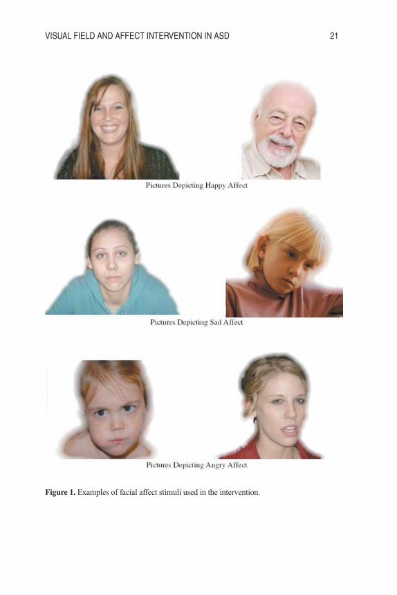
they included only head and shoulders against a white background (See Figure 1).
Biopac MP35 (Biopac Systems, Inc., 2007) was used to collect physiological data. A
photoplethysmograph finger wrap, sensitive to changes in blood flow, was plugged into the
acquisition unit via Channel 2. Pulse rate information was recorded from the non-dominant
index finger and was converted into visual form on a Toshiba Intel Centrino laptop computer
connected by USB to the Biopac acquisition unit. Pulse rate data was automatically saved
and was then converted into beats per minute units.
To achieve visual field isolation, a pair of children‘s sunglasses was modified. Original
lenses were taken out; the right eye was occluded using black construction paper to cover the
entire lens, which was then reinserted. The lateral portion of the left eye of the glasses was
covered with black construction paper, as well. Only the medial portion of the left eye was
open for sight, achieving right hemisphere visual pathway isolation. A pair of identical
children‘s sunglasses was modified for control group participants by removal of both lenses.
No further adjustments were made to these glasses.
DESIGN AND PROCEDUREThe present study was a simple, between-group experiment. Experimental and control
groups were equivalent, each including three elementary-school-aged boys diagnosed with
Autism Spectrum Disorder. Participants who had returned parental permission forms were
individually taken to a quiet area of their normal special education classroom. Teachers were
present in the room during the course of the experiment, so as to make participants as
comfortable as possible. The participants sat directly in front of the computer monitor and
were greeted by a recorded message explaining the procedure. After they assented, participants
were fitted with either the experimental or control glasses and the photoplethysmograph on
their self-reported non-dominant index finger.
Day 1Participants were led through practice block of the SuperLab program. They were asked
to match a happy, sad, and angry photograph with their respective emoticons. For each of the
three practice trials a stimulus picture appeared on screen for 2.5 seconds, followed
automatically by a response choice screen. The left third of the screen featured a “happy”
emoticon, the middle third a “sad” emoticon, and the right third a “mad” labeled emoticon.
A left mouse click in any of these three areas would elicit auditory feedback (prerecorded
message). If the participant made a successful match, he would hear “Correct.” If the
participant answered incorrectly, he would hear “Oops. That‘s incorrect. Pick a different
answer,” and then see the stimulus presented again before being allowed to correct the
answer. SuperLab would not progress to the next trial until the participant selected the
correct answer.
14 VISUAL FIELD AND AFFECT INTERVENTION IN ASD
GS019 JUR10_GS JUR text 1/11/11 11:41 AM Page 14

VISUAL FIELD AND AFFECT INTERVENTION IN ASD 15
Next, participants completed the baseline block, consisting of 45 matching trials comparable
to the ones they had done for practice. Fifteen pictures from each emotional category (happy,
sad, or mad) were presented in random order. SuperLab recorded accuracy and reaction
times of these baseline responses, while heart rate was recorded by Biopac.
Subsequently, participants completed the feedback block. This was the teaching portion
of the intervention, where participants completed the same matching task with 30 new
photographs. For each answer, participants heard “Correct” if they completed the trial
correctly or “Incorrect. Pick a different answer” if they made an incorrect match. The
computer program would show the trial stimulus again and progress to the next trial only
after the correct answer had been selected.
Finally, participants completed the no feedback block. This teaching portion utilized the
same 30 pictures used during the feedback block, except this time, participants were not told
after each trial whether their match was correct. The purpose of withholding feedback here
was to discourage the participants from becoming reliant on the feedback once they were
asked to complete the final block at the conclusion of three days of the teaching intervention.
Day 2Participants completed the feedback block in the same manner as Day 1. The no
feedback block was also presented in the same manner as day one. Accuracy, reaction time,
and pulse rate measurements were recorded but not saved.
Day 3Day 3 also began with the teaching feedback and no feedback blocks. Then, participants
were asked to again complete the 45 trials of the final block which was equivalent to the
baseline block. In this way, changes in accuracy, reaction time, and physiological reactions
from the start to conclusion of the intervention could be measured. A recorded debriefing
message explained the purpose of the experiment, prompted participants to ask the
experimenter questions if they had any, and thanked them for their participation. All
participants received a small prize upon completion of each of the three sessions, including
their choice of stickers, pencils, and pencil grippers. See Figure 2 for a complete diagram of
each day‘s procedures.
RESULTSAnalysis of baseline block measures confirms that there were no significant pre-existing
differences between groups in percent accuracy, t(4) = -.47, p = 0.66 (two-way).
Pre-intervention percent accuracy averaged across both experimental and control
groups, was 70%. There were negligible differences between the groups‘ baseline reaction
times, t(4) = .60, p = .58 (two-way), and baseline heart rates, t(4) = 1.36, p = .25 (two-way).
An alpha level of .05 was designated for this experiment.
Table 1 shows the baseline and final percent accuracy scores, as well as total changes in
percent accuracy for each participant. Participants in the experimental group showed an
average decrease in percent accuracy (M = -2.00%, SD = 21.68%), while participants in the
GS019 JUR10_GS JUR text 1/11/11 11:41 AM Page 15

16 VISUAL FIELD AND AFFECT INTERVENTION IN ASD
control group showed an average increase in percent accuracy (M = 7.41%, SD = 10%). The
change in accuracy shown by the experimental group did not differ significant from that
shown by the control group, t(4) = -.68, p = .53 (two-tailed). Notably, when the outlier
(participant three of the experimental group) was excluded from analysis, the experimental
group actually showed an average increase in percent accuracy (M = 10.33%, SD = 5.19%),
slightly greater that of the control group, though still not significant.
There were no significant differences between groups on average change in reaction
time, t(4) = -.33, p = .76 (two-tailed). The average improvement (decrease) in reaction time
(M = 54.82 ms, SD = 3209.86) for members of the experimental group over the course of the
intervention was less than average improvement shown by members of the control group (M= 670.73 ms, SD = 503.39). Again, if outlying data from participant three of the experimental
group is excluded from analysis, the experimental group showed an average improvement in
reaction time (M = 1680.39 ms, SD = 2179.82) greater than that of the control group, though
not significantly so, t(3) = .835, p = .465, (two-tailed).
Figure 3 shows that the heart rates of members of the experimental group declined across
trials (M = -3.67 BPM, SD = 15.05), whereas heart rates for the control group increased from
baseline to final measurement (M = 47.06, SD = 45.64). There was no significant difference
between the groups at the .05 level, t(4) = -1.83, p = .14 (two-tailed). If outlying data is
excluded from examination (participants 3 and 4), there is, in fact, a significant difference
between the mean change in heart rate shown by experimental participants (M = -11.70, SD= 8.16 and mean change in heart rate shown by control participants (M = 47.06, SD = 45.64),
t(2) = -10.73, p = .009, (two-tailed). That is, the average heart rate of experimental
participants dropped, while the average heart rate of control participants sped up.
DISCUSSIONIn contrast to the hypothesis that the group with visual isolation would show significant
improvement above that of the control group, no differences were found. In line with similar
studies of facial affect recognition in autistic populations (Silver & Oakes, 2001), in the
current study, the groups had a combined average of 70% accuracy at the beginning of the
first day of intervention. However, contrary to the hypothesis that the visual field isolation
group would demonstrate improvement in accuracy beyond the control group, the group‘s
average accuracy actually decreased. A likely explanation for the decrease in average percent
accuracy is the outlying data of one participant in the experimental group. This participant was
particularly vulnerable to frustration and on the day of final measurements, became visibly
irritated. When this data was excluded, the experimental group showed an improvement in
accuracy greater than that of the control group. Previous studies of similar intervention
programs have garnered mixed results. Lopata and colleagues (2008) also found no significant
change in accuracy on children‘s‘ ability to identify emotion, whereas Silver and Oakes
(2001) found modest improvements.
There are a few ways in which the present method could be improved to clarify changes
in accuracy: In the present study, one participant in the control group achieved near-perfect
accuracy on baseline and final measures, indicating a possible ceiling effect. Although some
GS019 JUR10_GS JUR text 1/11/11 11:41 AM Page 16

VISUAL FIELD AND AFFECT INTERVENTION IN ASD 17
research has indicated children with ASD have the most trouble with emotions of negative
valence such as anger and sadness included in the present study (Ashwin et al., 2006), others
have found that the most trouble comes with more complex emotions like embarrassment,
pride, and jealousy (Golan, Baron-Cohen, & Golan, 2008). Perhaps replacement of current
stimulus pictures with those of more complex emotions would assist in discrimination of
percent accuracy differences between groups. Additionally, although inter-rater reliability
was .80 for all pictures, some pictures were consistently mislabeled by most participants.
The mislabeled pictures were judged to be sad, but most children matched them to the mad
emoticon. These pictures should be discarded and replaced in future studies.
Both experimental and control groups showed improvement in processing speed by
decreasing their reaction times from baseline to final evaluation, though there were not
significant differences present. Again, the emotional lability and inattention of participant 3 in
the experimental group may misrepresent actual trends in reaction time. If this outlying data is
excluded, the experimental group achieved demonstrably faster reaction times than the control
group. While faster processing does not necessarily equate with better accuracy in processing
emotional stimuli, it does indicate a greater level of stimulus salience, which is an improvement
for children with autism, who tend to ignore faces (Krysko & Rutherford, 2009).
The findings of heart rate change in the present study are puzzling. Physiological
measures are thought to be a particularly valid measure of arousal because they theoretically
should not be affected by the communication impairments present in ASD and have been
shown to change relatively quickly with changes in affective state (Liu, Conn, Sarkar, &
Stone, 2008). According to Liu and colleagues, two minutes is the minimum amount of time
needed to confidently identify these changes; participants in the current study worked on the
baseline block and equivalent final block for more than two minutes. Therefore, physiological
changes induced by the emotion-laden photographs should have been detected in the current
study‘s participants.
Average heart rates, as measured by Biopac in the current experiment (M = 128.75 BPM,
SD = 27.73) were very high— higher than the 70-80 BPM expected in typically developing
individuals (Liu et al., 2008). Possible explanations for this discrepancy include evidence that
autistic children have naturally-higher pulse rates than typically developing children (James
& Barry, 1980). All of the participants in the present study demonstrated some anxious,
repetitive hand activity while recording took place, which likely artificially inflated their heart
rates. As this anxious activity took place on both the baseline block of trials and the final
block of trials, its effects on the ―change in heart rate data of each participant are negligible.
According to the results of the present researcher‘s past study, ASD individuals showed
significantly increased heart rate when viewing stimuli with their right visual field/left
hemisphere (Brindley & Schmidt, 2009). If in the present study, left visual field isolation
could condition the right hemisphere pathway, the experimental participants would have
shown the most increase in arousal to stimuli after practice. The contrary was actually true.
When outliers (Participants 3 and 4) were removed from their respective groups, the control
group showed a significantly greater increase in heart rate than the experimental group. It is
unclear why the control group improved more than the experimental group. Possibly, the
experimental group stopped paying attention to the stimuli when they were not allowed to
GS019 JUR10_GS JUR text 1/11/11 11:41 AM Page 17

18 VISUAL FIELD AND AFFECT INTERVENTION IN ASD
use their left hemisphere piecemeal strategy. This would fit well with hypothesis that autistic
individuals do not pay attention to faces, because they just do not understand them.
Clearly, there were a number of limitations in the present study. Five of the six
participants completed all three days of training, but due to illness, one of the children was able
to complete only two of the days. Participants generally accepted the photoplethysmograph
and glasses without irritation, although at times, participants would fidget with the glasses
and move their fingers. Another possible source of error is that some children had to be
periodically redirected back to the activity after they would get distracted or start to talk to
the examiner.
Though significant differences between groups were not found, each student showed
some level of improvement in accuracy and reaction time. It is important to interpret the
present findings in light of the fact that the sample size of each group was very small.
Additionally, there were severe time restrictions which allowed for only three days of the
teaching intervention. Most interventions have occurred over the course of months, not days
(Bryson, Rogers, & Fombonne, 2003; Lacava, Golan, Baron-Cohen, & Smith Myles, 2007;
Lopata et al., 2008; Silver & Oakes, 2001). Future research should greatly expand the
sample size. More time to teach would also allow for the most accurate understanding of
visual field isolation and its potential utility in teaching emotional affect comprehension to
children with ASD.
REFERENCESAdobe Systems, Inc. (2005). Adobe Photoshop Elements (Version 4.0) [Computer Software].
San Jose, CA: Adobe Systems Inc.
Ashwin, C., Chapman, E., Colle, L., & Baron-Cohen, S. (2006). Impaired recognition of
negative basic emotions in autism: A test of the amygdala theory. Social Neuroscience, 1(3-4), 349-363. doi: 10.1080/17470910601040772
Biopac Systems, Inc. (2007). Biopac Student Lab Pro (Version 3.7.2) [Computer software
and manual]. Goleta, CA: Biopac Systems, Inc.
Bö lte, S., Feineis-Matthews, S., & Poustka, F. (2008). Brief report: Emotional processing in
high-functioning autism—physiological reactivity and affective report. Journal of Autismand Developmental Disorders, 38, 776-781. doi: 10.1007/s10803-007-0443-8
Bourne, V. (2008). Chimeric faces, visual field bias, and reaction time bias: Have we been
missing a trick? Laterality: Asymmetries of Body, Brain and Cognition, 13(1), 92-103.
doi:10.1080/13576500701754315
Brindley, R., Schmidt, E. L. (2009). Differences in visual field bias for emotion recognitionin children with autism spectrum disorder and typical development. Manuscript
submitted for publication.
Bryson, S. E., Rogers, S. J., Fombonne, E. (2003). Autism spectrum disorders: Early
detection, intervention, education, and psychopharmacological management. CanadianJournal of Psychiatry, 48(8), 506-516.
Cedrus Corporation (2008). SuperLab 4.0 Stimulation Presentation Software (Version 4.0 7b)
[Computer software and manual]. San Pedro, CA: Cedrus Corporation.
GS019 JUR10_GS JUR text 1/11/11 11:41 AM Page 18

VISUAL FIELD AND AFFECT INTERVENTION IN ASD 19
Celani, G., Battacchi, M., & Arcidiacono, L. (1999). The understanding of the emotional
meaning of facial expressions in people with autism. Journal of Autism andDevelopmental Disorders, 29(1), 57-66. doi: 10.1023/A:1025970600181
Clark, T., Winkielman, P., & McIntosh, D. (2008). Autism and the extraction of emotion from
briefly presented facial expressions: Stumbling at the first step of empathy. Emotion, 8(6),
803-809. doi: 10.1037/a0014124
Cox, D., Meyers, E., & Sinha, P. (2004). Contextually evoked object-specific responses in
human visual cortex. Science, 304(5667), 115-117. doi: 10.1126/science.1093110
Deeley, Q., Daly, E., Surguladze, S., Page, L., Toal, F., Robertson, D., et al. (2007). An event
related functional magnetic resonance imaging study of facial emotion processing in
Asperger syndrome. Biological Psychiatry, 62(3), 207-217. doi:10.1016/j.biopsych.
2006.09.037
Dreamstime Free Images. (2009). Retrieved from http://www.dreamstime.com/free-photos.
Gauthier, I., Tarr, M. J. (2002). Unraveling mechanisms for expert object recognition:
Bridging brain activity and behavior. Journal of Experimental Psychology, 28(2), 431-446.
doi: 10.1037//0096-1523.28.2.431
Golan, O., Baron-Cohen, S., Golan, Y. (2008). The ‗Reading the Mind in Films‘ task [child
version]: Complex emotion and mental state recognition in children with and without
autism spectrum conditions.
Grelotti, D., Gauthier, I., & Schultz, R. (2002). Social interest and the development of cortical
face specialization: What autism teaches us about face processing. DevelopmentalPsychobiology, 40(3), 213-225. doi:10.1002/dev.10028
Grelotti, D., Klin, A., Gauthier, I., Skudlarski, P., Cohen, D., Gore, J., et al. (2005). fMRI
activation of the fusiform gyrus and amygdala to cartoon characters but not to faces in a
boy with autism. Neuropsychologia, 43(3), 373-385. doi: 10.1016/j.neuropsychologia.
2004.06.015
Hadjikhani, N., Joseph, R., Snyder, J., Chabris, C., Clark, S., McGrath, L., et al. (2004).
Activation of the fusiform gyrus when individuals with autism spectrum disorder view
faces. NeuroImage, 22, 1141-1150. doi: 10.1016/j.neuroimage.2004.03.025
James, A. L., & Barry, R. J. (1980). Respiratory and vascular responses to simple visual
stimuli in autistics, retardates and normals. Psychophysiology, 17, 541-547.
Kanwisher, N., Stanley, D., & Harris, A. (1999). The fusiform face area is selective for faces
not animals. NeuroReport, 10, 183-187.
Krysko, K. M., Rutherford, M. D. (2009). A threat-detection advantage in those with autism
spectrum disorders. Brain and Cognition, 69(3), 472-80. doi: 10.1016/j.bandc.2008.
10.002
Lacava, P. G., Golan, O., Baron-Cohen, S., & Smith Myles, B. (2007). Using assistive
technology to teach emotion recognition to students with Asperger syndrome. Remedialand Special Education, 28(3), 174-181. doi: 10.1177/07419325070280030601
Liu, C., Conn, K., Sarkar, N., & Stone, W. (2008). Physiology-based affect recognition for
computer-assisted intervention of children with Autism Spectrum Disorder. InternationalJournal of Human-Computer Studies, 66(9), 662-677. doi:10.1016/j.ijhsc.2008.04.003
Lopata, C., Thomeer, M. L., Volker, M. A., Nida, R. E., & Lee, G. K. (2008). Effectiveness
of a manualized summer social treatment program for high-functioning children with
GS019 JUR10_GS JUR text 1/11/11 11:41 AM Page 19

20 VISUAL FIELD AND AFFECT INTERVENTION IN ASD
autism spectrum disorders. Journal of Autism and Developmental Disorders, 38, 890-904.
doi: 10.1007/s10803-007-0460-7
Minnebusch, D. A. (2009). A bilateral occipitotemporal network mediates face perception.
Behavioral Brain Research 198, 179-185. doi:101016/j.bbr.2008.10.041
Nijokiktjien, C., Verschoor, A., de Sonneville, L., Huyser, C., Op het Veld, V., & Toorenaar,
N. (2001). Disordered recognition of facial identity and emotions in three Asperger type
autists. European Child and Adolescent Psychiatry, 10 (1), 79-90. doi:
10.1023/A:1024458618172
Pierce, K., Muller, R., Ambrose, J., Allen, G., & Courchesne, E. (2001). Face processing
occurs outside the fusiform 'face area' in autism: Evidence from functional MRI. Brain,124 (10), 2059-2073. Retrieved January 27, 2009, from Biological Abstracts database.
Piggot, J., Kwon, H., Mobbs, D., Blasey, C., Lotspeich, L., Menon, V., et al. (2004). Emotional
attribution in high-functioning individuals with autistic spectrum disorder: A functional
imaging study. Journal of the American Academy of Child & Adolescent Psychiatry, 43(4), 473-480. Retrieved January 20, 2009, doi:10.1097/01.chi.0000111363. 94169.37
Schultz, R., Grelotti, D., Klin, A., Kleinman, J., Van der Gaag, C., Marois, R., et al. (2003).
The role of the fusiform face area in social cognition: Implications for the pathobiology
of autism. Philosophical Transactions of The Royal Society B, 358, 415-427. Retrieved
February 17, 2009 from http://rstb.royalsocietypublishing.org/
Silver, M., & Oakes, P. (2001). Evaluation of a new computer intervention to teach people
with autism or Asperger syndrome to recognize and predict emotions in others. Autism, 5(3), 299-316. doi: 10.1177/1362361301005003007
Van Kooten, I. A. J., Palmen, S. J. M. C., von Cappeln, P., Steinbusch, H. W. M., Korr, H.,
Heinsen, H., …et al. (2008). Neurons in the fusiform gyrus are fewer and smaller in
autism. Brain, 131, 987-999. doi: 10.1093/brain/awn033
Wang, T., Dapretto, M., Hariri, A., Sigman, M., & Bookheimer, S. (2004). Neural correlates
of facial affect processing in children and adolescents with autism spectrum disorder.
Journal of the American Academy of Child and Adolescent Psychiatry, 43 (4), 481-489.
Yovel, G., Tambini, A., & Brandman, T. (2008). The asymmetry of the fusiform face area is a
stable individual characteristic that underlies the left-visual-field superiority for faces.
Neuropsychologia, 46 (13), 3061-3068. doi:10.1016/j.neuropsychologia.2008.06.017
Table 1:Percent Accuracy by Participants Across Three Days of Affect-Learning Activity
Group Participant Baseline Final Percent Accuracy
Experimental 1 0.67 0.80 0.14
2 0.62 0.69 0.07
3 0.71 0.44 -0.27
Control 4 0.93 0.91 -0.02
5 0.47 0.64 0.18
6 0.80 0.87 0.07
GS019 JUR10_GS JUR text 1/11/11 11:41 AM Page 20
VISUAL FIELD AND AFFECT INTERVENTION IN ASD 21
Figure 1. Examples of facial affect stimuli used in the intervention.
GS019 JUR10_GS JUR text 1/11/11 11:41 AM Page 21

22 VISUAL FIELD AND AFFECT INTERVENTION IN ASD
Figure 2. Three-day intervention design and measurements.
Figure 3. Mean (SD) change in heart rate (BPM) for the experimental group (n =3), and control
group (n = 3) across three days of practice on a matching task of facial affective stimuli.
GS019 JUR10_GS JUR text 1/11/11 11:41 AM Page 22

PARENTAL INFLUENCE ON THE FINANCIAL LITERACY OF THEIR CHILDREN 23
Parental Influence on the FinancialLiteracy of Their School-Aged Children:An Exploratory Study
Author: Stephanie WilliamsFaculty Sponsor: Soo Hyun Cho, Ph.D.Department: Consumer Sciences
ABSTRACTThe purpose of this research is to assess the parental perception about their financial
habits and their children’s. This research was conducted through interviews, which were
administered through email, on the phone, or in person, in October 2009.
Financial literacy, promoting proper knowledge and habits, is very important in
sustaining a healthy economy and in achieving a good personal financial situation. Danes
(1994) points out that parents play an essential role in transferring knowledge of the realistic
and sensitive aspects of money. Mandell (2009) states that the use or misuse of financial
knowledge can affect an entire national economy. Clearly, more financial education is
necessary for young adults to better the economy. The family is the source for most of a
child’s financial knowledge. However, parents seem to pass only their own feelings about
money on to their children. If more parents could factually educate their children about
finance, children may be less likely to develop poor habits. If enough young adults entered
the adult world with sound financial literacy, it could have a macroeconomic effect.
INTRODUCTIONToday’s level of personal financial literacy in young adults has declined. More than
ever, people now live so far outside of their means that they cannot efficiently manage their
debts. The occurrence of bankruptcy has skyrocketed in the last twenty years. People so
often purchase items on credit; perhaps they have forgotten the value of their money. Poor
choices stem from a lack of knowledge, and finances are no exception. Since 1997, the
Jump$tart Coalition for Personal Financial Literacy has studied the financial literacy of high
school students. Mandell (2009) reported that the 2008 results of these surveys fell to the
lowest ever. The average survey score of 2008 was 48.3%; and 57.3% in 1997-98.
Researchers hoped that the initial failing grade in 1997-98 would rise over time, but the
opposite took place. Mandell (2009) deduced that an overwhelming 75% of young adults do
not have the knowledge to perform well financially. “Financial literacy clearly has ongoing
macroeconomic ramifications,” (Mandell, 2009, p. 6).
Some researchers focused a large portion of their study of this topic on college-aged
students. Thus, few studies show the financial aptitude of younger children. More research
on the young children and the early source of poor financial habits would prove beneficial.
GS019 JUR10_GS JUR text 1/11/11 11:41 AM Page 23

24 PARENTAL INFLUENCE ON THE FINANCIAL LITERACY OF THEIR CHILDREN
College students surveyed in past research thought back to their family and home life and
accounted for their financial education from their parents. However, this remains anecdotal
and unquantifiable information. More concrete results would stem from studying young
children and their parents to form a more valid and reliable description of reasons why some
families do not adequately teach their children about finance.
Beverly & Burkhalter (2005) found that research establishes that young people’s
knowledge of finance is lacking and many do not use optimal financial skills. This statement
generalizes current research on this topic. Nevertheless, it seems that researchers have not
thoroughly written on this topic as there are only a limited number of articles available.
Considering the research found, the common conclusion is that children and young adults
desperately need more financial education so they can make more informed decisions
as adults.
Researchers have conducted studies on the parental role of a child’s financial education.
The trend in research demonstrates that a child’s most significant source of financial
knowledge comes from their family. Danes (1994) points out that parents play an essential
role in transferring knowledge of the realistic and sensitive aspects of money. The family,
then, must realize this and act accordingly. Clarke, Heaton, Israelsen, & Eggett (2005)
argued that a very small amount of research exists pertaining to the passing of information
from parent to child about adult roles and responsibilities, particularly about finances. After
reviewing past research, it is evident that more research is necessary to see how parents
effectively communicate financial messages to their children.
Adolescents in particular experience difficulty in receiving proper financial guidance.
Many parents do not feel that they can influence their teenage child’s spending habits due to
peer influence. Furthermore, many teenagers have a high spending rate when using cash,
checks, or credit cards. Pinto, Parente, & Mansfield (2005) established that the age at which
young adults receive credit cards is dropping. As children have access to more money and
credit at a younger age, the need to ensure a quality financial education increases. Clarke, et
al. (2005) found that if teens have not received proper financial education from their parents,
they are likely to have unrealistic income aspirations and unwise financial habits.
Families provide the most deep-seated education. Clarke, et al. (2005) found that the
poor financial habits of parents commonly present themselves in their children’s lives.
Children watch and model their parental figures. From birth until they leave home, children
look to their parents for guidance and knowledge of the world. Clarke, et al. (2005)
explained that parents have a duty to educate and guide their children into taking on mature
responsibilities and tasks. They play the role of primary educator in a child’s life. Parents
themselves may not feel comfortable with their own financial situation so they do not want
to talk about it with their children. Edwards, Allen, & Hayhoe’s (2005) research found that
young adults are more reserved about discussing their personal finances with parents who (a)
have a fixation with money, (b) associate money with authority, and (c) make unwise
budgetary and savings decisions. Parents must establish good lines of communication with
their children about several aspects of the adult world, especially finance.
Young people must learn about financial responsibility before they develop lasting poor
habits. Bowen & Jones (2006) emphasize that young adults who lack education in matters of
personal finance will eventually have the control of our nation’s financial culture. The
general economy may improve by simply helping children learn about money at an early
GS019 JUR10_GS JUR text 1/11/11 11:41 AM Page 24

PARENTAL INFLUENCE ON THE FINANCIAL LITERACY OF THEIR CHILDREN 25
age. Clarke, et al. (2005) suggests that young adults feel more equipped to handle financial
responsibilities if they acquired a good education on the subject at home. This shows that the
best education starts at home. As research has indicated, families should place high priority
on teaching children about finances and the associated future adult responsibilities.
Schools also play a part in a child’s financial education, though a less significant part
than parents. Pinto, Parente, & Mansfield (2005) have observed that after a child starts
kindergarten, most of that child’s time will be spent within the school. The school system
provides an effective way to reach children and teach them about personal finance.
Unfortunately, many states do not require that schools incorporate finance into their
curriculum. Green (2009) clarifies that in the last five years, seventeen states have made
personal finance mandatory in their educational programs. She adds that only in Missouri,
Tennessee, and Utah, students have to take a course specifically covering personal finance.
Two websites in particular have begun trying to promote financial education in schools:
Jump$tart Coalition (http://www.jumpstart.org) and National Endowment for Financial
Education’s High School Financial Planning Program (http://hsfpp.nefe.org). These sites
provide free and low cost educational tools for all ages to learn about personal finance.
Though some schools across the country have begun incorporating financial education, it
still does not have the impact that parents do. Furthermore, according to Mandell (2009),
students who take a financial class in high school receive similar scores on the Jump$tart
Coalition survey as students who do not. This proves that the financial courses in schools
may not actually have a substantial effect.
Among all ages, harmful financial practices are on the rise in America. Edmiston (2006)
identified that five times more people are filing for bankruptcy than in 1980. Likewise,
comparing the FDIC Press Release (2010) and Reinsdorf’s (2007) statistics, it is evident that
personal savings rates are currently more than six percent lower than in the early 1980s. As
stated by Mandell (2009), three quarters of America’s young adults do not have an adequate
amount of financial knowledge. His data exemplifies that financial illiteracy leads to more
individuals making poor decisions in their money management. Mandell (2009) has also
stated that the use or misuse of financial knowledge can affect an entire national economy.
The rate that individuals save their money lacks promise. In a February 2007 report by
the Bureau of Economic Analysis, Reinsdorf (2007) shows the highest rate of personal savings
occurred in the mid-1940s at over 25% of income. This report also shows that in 2005 and
2006 the savings rate dropped to a negative number. Fortunately the savings rate has risen,
but only to a meager 4.6% in 2009, as a February 2010 press release by the Federal Deposit
Insurance Corporation confirms. Personal savings rates are so low that it seems as if people
do not have necessary concern for their future. Clearly, an underlying cause of all these
problems is a lack of financial literacy. More financial education is necessary for young
adults to better the economy.
Financial literacy, promoting proper knowledge and habits, remains important in
sustaining a healthy economy and in achieving a good personal financial situation. When
young people learn about finance, they will take those skills and habits with them into their
adult years. As children best learn about adult responsibilities from their parents and home-
life while growing up, it is important to study the transfer of financial knowledge from parent
to child. This research assesses the parental perception not only about their financial habits
but also their children’s.
GS019 JUR10_GS JUR text 1/11/11 11:41 AM Page 25

METHODSThe research for this paper was conducted using interview questionnaires given to
parents through phone, e-mail, and in-person (see Appendix A). Six of the ten interviewees
were from Gregory County, SD; and the other four were from Brookings, SD. E-mails were
sent to the parents of 5th graders in Gregory County; and one phone interview was given to a
parent there. Three parents in Brookings were interviewed by e-mail and one in person.
These interviews were all conducted between October 12th and 14th, 2009.
Basic demographic questions asked were: age, income, number and age of children, and
marital status. A scale was given so the participants could choose their bracket for age and
income. Marital status was selected between single and married. The children’s information
was simply filled in by the participant.
The core questions in the interview were left open-ended to permit various responses.
Creswell (2003) explains that the open-ended data leads to a qualitative analysis of the
results. Creswell (2003) also describes qualitative research as open to explanation–implying
that the interviewer provides their own understanding of the responses. The first questions
asked about the participant’s ease and frequency in addressing their children about financial
matters; and then asked for elaboration. Next, these questions addressed the participant’s
own financial beliefs compared with that of their children. The last question asked about
what could potentially benefit their children’s financial futures.
RESULTSThe compiled demographics appear in Table 1. Seven participants are married and three
are single. Seven are aged in their thirties, and three are in their forties. The average
household income of participants is between $40,000 and $49,000. Three participants
reported a household income of $0-$19,000 and five reported the highest income of $60,000+.
The median age of the participants’ children is eleven years, ranging from two to nineteen.
The median number of children in the participants’ families is three, ranging from two to six.
Table 1: Participants characteristics
26 PARENTAL INFLUENCE ON THE FINANCIAL LITERACY OF THEIR CHILDREN
GS019 JUR10_GS JUR text 1/11/11 11:41 AM Page 26

The responses to the core questions were compared to each other and some prominent
findings were discovered. Corresponding figures appear in Appendix B.
All four of the single participants only talk to their children about finances ‘Sometimes’,
as well as one married participant. The remaining six married participants talk with their
children ‘Often’ or ‘Very Often’ about finances (see Appendix B, Figure B1).
Seven of the participants feel comfortable talking about finance with their children.
They all explain that they do so to build their children’s knowledge of finance so they can
apply it properly when they are older. Three participants are not at all or only somewhat
comfortable talking to their children about finance. They each had different reasons: the
parents themselves feel negative about their financial situation, the children do not understand
finance, or the parent does not want to stress their children with financial matters (see
Appendix B, Figure B2).
When asked how they could increase the amount of time they talk to their children
about finances, the participants responded in a few different ways. Three participants said
they would simply need to find time to address this matter. Four responded they are unsure.
The other three participants responded as follows: do nothing, engage the children as
appropriate by age and situation, and make them work more for their money (see Appendix
B, Figure B3).
Six of the participants felt that saving money was very important. However, only three
felt that their children held the same value (see Appendix B, Figure B4). Only two
participants felt very confident in their own financial decisions; four were not very confident
and four were somewhat confident. Likewise, only two felt very confident in their children’s
financial decisions; three were not very confident and five were somewhat confident (see
Appendix B, Figure B5).
The last question, addressing what participants think will best benefit their child’s
financial future, produced a variety of responses. Some participants responded with more
than one option of ways to help their children’s financial future. Of the ten participants, five
responded with just one idea, four responded with two ideas, and one responded with three
ideas; creating a total of 16 total responses. The most frequent answer that appeared in eight
participant responses was parental influence, or education from home. The other two
answers received four responses each: financial education in a school classroom setting, and
learning from real world experiences (see Appendix B, Figure B6).
CONCLUSIONSThis research was conducted to learn about personal financial literacy passing from
parent to child. It was to show frequency, effectiveness, and a correlation, if any, to lifestyle
and personal beliefs. The research shows, on a small scale, what may commonly occur
among America’s population.
The supporting idea of this research is that a parent’s personal feelings about finance
determine how they pass financial information to their child. The participants who felt
comfortable talking with their children about financial matters do so because they want their
children to have strong knowledge of personal finance to help with a better future. The
participants who do not feel comfortable talking with their children about financial matters
PARENTAL INFLUENCE ON THE FINANCIAL LITERACY OF THEIR CHILDREN 27
GS019 JUR10_GS JUR text 1/11/11 11:41 AM Page 27

either do not understand it themselves, think their children will not understand it, or they do
not want their children to stress about it. Two of the three participants who do not feel
comfortable talking with their children about financial matters also responded that they are
not very confident in their own financial decisions and do not regard saving money as
important. The third is only fairly confident in personal financial decisions and is not likely
to save money. These results reveal parents who are passing their own feelings about money
on to their children.
Other research has also come to this conclusion. Pinto, Parente, and Mansfield (2005,
p. 360), presented findings by Cohen & Xiao (1992) and Hira (1997): “financial attitudes
and spending behavior … are thought to be transmitted by parents and other influential
individuals.” Furthermore, Clarke, et al. (2005) explained that the poor financial habits of
parents commonly present themselves in their children’s lives.
Parental guidance in financial matters is of primary importance. Children learn the most
from home. Also, as the results show, parents themselves realize their importance in their
children’s education. Eight of the ten participants interviewed responded that more
interaction from them would help most with their children’s financial education and future.
Knowing this, there should be more emphasis on parents to help their children understand
personal finance.
The connection between lifestyle and financial capability of parents and children is
evident in the research. All of the three single participants, who are also the only three in the
lowest household income bracket, are the least likely to have financial confidence in
themselves and their children. Also, these three participants and their children are the least
likely to understand the importance of saving their money. Single working parents do not
always have much quality time to spend with their children. This lack of time with their
children implies reason for the lack of financial education at home. On the contrary, the four
married participants in the highest reported income bracket are the most likely to have
financial confidence in themselves and their children. These participants and their children
are also the most likely to understand the importance of saving their money and actually
practice it. The same conclusion arises in Mandell’s (2009) results: students with parents
who earn a higher income are likely to score higher on the Jump$tart Coalition survey.
Another observation from the research shows that parents hold different views of when
the right time is to teach their children about finance. Some participants only talked about
financial matters to their children of upper-teenage years. Half of all the participants made
age based comments in some of their responses. They talk with the older children about
finance but not the younger. They do not think it is necessary to teach their children about
finance until a later age. On the contrary, one participant in particular has children ages six
and seven who are already learning about spending and saving and price comparison. The
perception of a child’s preparedness to learn about finance definitely varies from household
to household. If more parents started educating their children earlier about finance, the
children may be less likely to develop the poor habits in their early years.
The family is the source of a majority of a child’s financial knowledge. This is reflected
in other research studies as well as in these results. Pinto, Parente, & Mansfield (2005) offer
one reference to this: Children in America feel that most of their financial knowledge came
from their parents. Although most of the participants admit that they should be the ones
28 PARENTAL INFLUENCE ON THE FINANCIAL LITERACY OF THEIR CHILDREN
GS019 JUR10_GS JUR text 1/11/11 11:41 AM Page 28

teaching their children about financial matters, many of them still don’t have an active
involvement with their children on the issue. There must be a way to awaken the parents that
are least likely to have financial confidence and financial knowledge; and to help them learn
and teach their children. Modern theorists and cultural philosophers agree that parents have a
duty to educate and guide their children into taking on mature responsibilities and tasks, as
Clarke, et al. (2005) found.
LIMITATIONSThe small number of people interviewed is a limitation. A more thorough collection of
data could have been found if more people were interviewed. Also, if more were interviewed
from other parts of the state or regions of the country it would give a more broad perspective.
A sampling bias is evident as some of the parents who received the interview e-mail might
have not responded. Parents who themselves are not comfortable with personal finance may
not have responded to the e-mail survey. This limitation is characterized by the unlikelihood
of people to freely give information that they are not comfortable with. Also, some families
may simply be more private about their financial information.
ACKNOWLEDGEMENTSI would like to thank Dr. Soo Hyun Cho, in the Department of Consumer Sciences, for
assistance, guidance, and support on this research project. Also, I would like to thank Dr. John
Taylor, in the English Department, for aid with revisions and APA formatting.
REFERENCESBeverly, S. G., & Burkhalter, E. K. (2005). Improving the financial literacy and practices of
youths. Children & Schools, 27 (2), 121-124. Retrieved from http://www.cinahl.com/
cgi-bin/refsvc?jid=1907&accno=2005107340
Bowen, C. F., & Jones, H. M. (2006). Empowering young adults to control their financial
future. Journal of Family and Consumer Sciences, 98 (1), 33-39. Retrieved from
http://proquest.umi.com/pqdweb?did=991647971&sid=1&Fmt=4&clientId=44583&RQ
T=309&VName=PQD
Clarke, M. C., Heaton, M. B., Israelsen, C. L., & Eggett, D. L. (2005). The acquisition of
family financial roles and responsibilities. Family and Consumer Sciences ResearchJournal, 33 (4), 321-340. Retrieved from http://fcs.sagepub.com/cgi/reprint/33/4/321.pdf
Creswell, John W. (2003). Research Design: Qualitative, Quantitative, and Mixed Method(2nd ed.). Thousand Oaks, CA: Sage Publications
Danes, Sharon M. (1994). Parental Perceptions of Children’s Financial Socialization. Journalof Financial Counseling and Planning. Vol. 58, 127-149. Retrieved from
http://6aa7f5c4a9901a3e1a1682793cd11f5a6b732d29.gripelements.com/pdf/vol-58.pdf
PARENTAL INFLUENCE ON THE FINANCIAL LITERACY OF THEIR CHILDREN 29
GS019 JUR10_GS JUR text 1/11/11 11:41 AM Page 29

30
Edmiston, Kelly D. (2006). A New Perspective on Rising Nonbusiness Bankruptcy Filing
Rates: Analyzing the Regional Factors. Economic Review - Federal Reserve Bank ofKansas City, 91 (2), 55-74. Retrieved from http://www.kc.frb.org/PUBLICAT/
ECONREV/PDF/2Q06edmin.pdf
Edwards, R., Allen, M., & Hayhoe, C. (2007). Financial attitudes and family communication
about students’ finances: The role of sex differences. Communication Reports, 20 (2),
90-100. doi:10.1080/08934210701643719
Federal Deposit Insurance Corporation. (2010). FDIC Calls Upon Consumers to Save andBuild Wealth. Retrieved from http://www.fdic.gov/news/news/press/2010/pr10035.html
Green, A. (2009, March 9). Push for financial literacy spreads to schools. Christian ScienceMonitor, p. 13. Retrieved from http://www.csmonitor.com/Money/2009/0309/
p13s01-wmgn.html
Jump$tart Coalition for Personal Financial Literacy website: http://www.jumpstart.org/
Mandell, Lewis. (2009). The Financial Literacy of Young American Adults. Retrieved from
the Jump$tart Coalition for Personal Financial Literacy website:
http://www.jumpstart.org/upload/2009_FinLit-Mandell.pdf
National Endowment for Financial Education’s High School Financial Planning Program
website: http://hsfpp.nefe.org/
Pinto, M. B., Parente, D. H., & Mansfield, P. M. (2005). Information learned from
socialization agents: Its relationship to credit card use. Family and Consumer SciencesResearch Journal, 33 (4), 357-367. http://ejournals.ebsco.com/direct.asp?ArticleID=
4540A581A5BA565ED78F
Reinsdorf, Marshall B. (2007). Alternative Measures of Personal Saving. Retrieved from
http://www.bea.gov/scb/pdf/2007/02%20February/0207_saving.pdf
APPENDIX A - INTERVIEW QUESTIONS1) How many children do you have? _________
2) Are you a single parent or are you married? Single; Married3) What is your age? 18-29; 30-39; 40-49; 50-59; 60+4) What are the ages of your children? _________
5) What is your household income? $0-$19,000; $20,000-$29,000; $30,000-$39,000;$40,000-$49,000; $50,000-$59,000; $60,000+
6) Do you feel comfortable talking with your children about financial matters?
a) Why?
b) Does your spouse?
7) How frequently do you and/or your spouse talk to your children about money?
Very Often (2+ times/week); Often (once/week); Sometimes (1-2 times/month); Rarely (1-3 times/year); Nevera) Do you think this is enough?
b) What can you do to increase the number of times you talk to your children about money?
8) How important is saving money to you and/or your spouse?
9) How well do your children understand the importance of saving money?
10) How confident are you in your own financial decisions?
30 PARENTAL INFLUENCE ON THE FINANCIAL LITERACY OF THEIR CHILDREN
GS019 JUR10_GS JUR text 1/11/11 11:41 AM Page 30

31
11) How confident are you in your children’s financial decisions?
12) What do you feel would help your children most with financial education and their
financial future?
APPENDIX B – FIGURESFigure B1: How frequently do you and/or your spouse talk to your children about money?
Figure B2: Do you feel comfortable talking with your children about financial matters?
PARENTAL INFLUENCE ON THE FINANCIAL LITERACY OF THEIR CHILDREN 31
GS019 JUR10_GS JUR text 1/11/11 11:41 AM Page 31

Figure B3: What can you do to increase the number of times that you talk with your children
about money?
Figure B4: How important is saving money to you and/or your spouse? How well do your
children understand the importance of saving money?
32 PARENTAL INFLUENCE ON THE FINANCIAL LITERACY OF THEIR CHILDREN
GS019 JUR10_GS JUR text 1/11/11 11:41 AM Page 32

33PARENTAL INFLUENCE ON THE FINANCIAL LITERACY OF THEIR CHILDREN 33
Figure B5: How confident are you in your own financial decisions? How confident are you
in your children’s financial decisions?
Figure B6: What do you feel would help your children most with financial education and
their financial future?
GS019 JUR10_GS JUR text 1/11/11 11:41 AM Page 33

35FORMULA SAE INPACT ATTENUATOR TESING 35
Formula SAE Impact Attenuator Testing
Authors: Chad Abrahamson, Bill Bruns, Joseph Hammond, Josh Lutter
Faculty Sponsor: Dr. Shawn DuanDepartment: Mechanical Engineering
ABSTRACTThe purpose of this paper is to validate the impact attenuator designed by SDSU
Formula SAE team according to 2010 Formula SAE rules. The impact attenuator is made of
Plascore PCGA-XR1-5.2-1/4-P-3003 aluminum honeycomb that is pre-crushed to 245 psi.
The test was dynamically performed using a 661 lb mass dropped 8.3 ft onto the material
sample at 23 ft/sec, and data was measured with an Olympus i-SPEED 3 high speed camera.
The impact attenuator must have an average deceleration equal to or less than 20 G’s and a
peak deceleration equal to or less than 40 G’s. Two specimens were tested. The physical
dimensions of the first specimen are 10 inches long by 8 inches wide by 5 inches tall. Data of
the first sample showed a peak deceleration of 46.88 G’s and an average deceleration of
17.86 G’s. The velocity at impact was above 24ft/sec. The second specimen is 10 inches long
by 10 inches wide by 4 inches tall. The second sample had a peak deceleration of 36.2 G’s
and an average deceleration of 14 G’s. The velocity at impact was slightly above 23ft/sec.
The first sample was unacceptable and the second specimen was acceptable under the
guidelines set forth by Formula SAE Rule B.3.21.1.
INTRODUCTIONFormula SAE is a student design competition organized by the Society of Automotive
Engineers. In the mid 1970s, several universities began hosting local student design
competitions with off-road vehicles called SAE Mini Bajas. At one of the competitions, Fred
Stratton, from the Briggs & Stratton Corporation (B&S), was a design judge. After judging
the competition, there was a strong connection with SAE and B&S. A few years after the
Mini Baja gained popularity, members developed the idea of a road race instead of off-road
and so the SAE Mini Indy was born in 1978.
The experiments performed in this paper will focus on the impact attenuator required
by the 2010 Formula SAE Rules. To understand the type and design of the vehicle in
question, South Dakota State University’s 2009 Formula SAE Car is presented in Figure 1.
The impact attenuator is located under the front of the nosecone.
GS019 JUR10_GS JUR text 1/11/11 11:41 AM Page 35
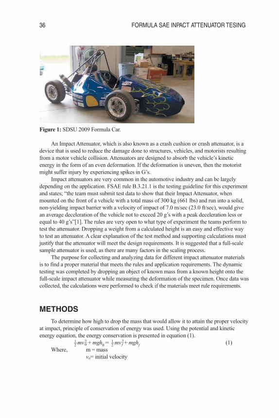
Figure 1: SDSU 2009 Formula Car.
An Impact Attenuator, which is also known as a crash cushion or crash attenuator, is a
device that is used to reduce the damage done to structures, vehicles, and motorists resulting
from a motor vehicle collision. Attenuators are designed to absorb the vehicle’s kinetic
energy in the form of an even deformation. If the deformation is uneven, then the motorist
might suffer injury by experiencing spikes in G’s.
Impact attenuators are very common in the automotive industry and can be largely
depending on the application. FSAE rule B.3.21.1 is the testing guideline for this experiment
and states; “the team must submit test data to show that their Impact Attenuator, when
mounted on the front of a vehicle with a total mass of 300 kg (661 lbs) and run into a solid,
non-yielding impact barrier with a velocity of impact of 7.0 m/sec (23.0 ft/sec), would give
an average deceleration of the vehicle not to exceed 20 g’s with a peak deceleration less or
equal to 40 g’s”[1]. The rules are very open to what type of experiment the teams perform to
test the attenuator. Dropping a weight from a calculated height is an easy and effective way
to test an attenuator. A clear explanation of the test method and supporting calculations must
justify that the attenuator will meet the design requirements. It is suggested that a full-scale
sample attenuator is used, as there are many factors in the scaling process.
The purpose for collecting and analyzing data for different impact attenuator materials
is to find a proper material that meets the rules and application requirements. The dynamic
testing was completed by dropping an object of known mass from a known height onto the
full-scale impact attenuator while measuring the deformation of the specimen. Once data was
collected, the calculations were performed to check if the materials meet rule requirements.
METHODSTo determine how high to drop the mass that would allow it to attain the proper velocity
at impact, principle of conservation of energy was used. Using the potential and kinetic
energy equation, the energy conservation is presented in equation (1).1–2
mv20 + mgh
0= 1–
2mv2
f + mghf (1)
Where, m = mass
vo= initial velocity
36 FORMULA SAE INPACT ATTENUATOR TESING
GS019 JUR10_GS JUR text 1/11/11 11:41 AM Page 36

g = gravity
ho= initial height
Vf= final velocity
hf= final height
Defining the final position, when the mass impacts the attenuator, the right hand side of
the equation can be reduced by stating the final height is equal to zero. The left hand side of
the equation is reduced by recognizing that the mass has an initial velocity of zero. The mass
in the equation is the same for each term so it is divided at both sides of equation (1). Then
equation (1) is reduced to the equation presented in equation (2). Solving Equation 2 for
initial height gives equation (3).
gh0
= 1–2
v2f (2)
h0
= 1–2g v2
f (3)
In order to find the deceleration of the mass, data was taken from an Olympus i-SPEED
3 high speed camera. The camera was set to capture pictures at a rate of 7500 frames per
second. A checkered pattern placed on the barrel provided the data analyzer with a known
pixel per inch to calculate the speed of the barrel before and during impact. The video
collected by the camera was analyzed frame by frame. Knowing the frames per second and
the distance that the barrel fell per frame of video gives the velocity of the barrel, which is
the change in distance per time. Deceleration is the change in velocity per time, so using the
data calculated from the camera the deceleration of the barrel was found over the crushing of
the impact attenuator.
To test the impact attenuator for the 2009-2010 South Dakota State University formula
car, the team designed the model presented in Figure 2. The structure is modeled to have at
least 8.2 feet between the bottom of the falling mass and the top of the impact attenuator so
that the mass will attain the proper velocity at impact. The mass is a 30 gallon barrel filled full
with concrete. I-bolts were inserted in the sides of the barrel to use for lifting if necessary.
A half inch aluminum plate was placed on the frozen ground as a platform. Testing was
performed in the middle of winter when the temperature outside was well below freezing to
minimize the energy absorbed by the ground. The structure design is modeled around the
overhead hoist available for use at South Dakota State
University. The impacting mass is attached to the
overhead hoist with a rope. The rope is cut to release the
mass from the overhead hoist allowing the mass to fall on
the impact attenuator.
The overhead hoist and all components of the
testing procedure are presented in Figure 3. The
aluminum plate was centered under the impacting mass
using a plumb bob. The barrel was fitted with a checkered
pattern so the high speed camera would have sufficient
points for data recovery. The high speed camera was
placed approximately 10 feet from the impact attenuator.
When the mass was released the camera operator pressed
a button to capture the process.
FORMULA SAE INPACT ATTENUATOR TESING 37
Figure 2: Model of Testing Method.
GS019 JUR10_GS JUR text 1/11/11 11:41 AM Page 37

38 FORMULA SAE INPACT ATTENUATOR TESING
Figure 3: Overhead Hoist and Testing Components.
After capturing the process with the camera, the data was analyzed using i-SPEED
Control Pro Software. A screen shot of the software during analysis of the testing is
presented in Figure 4. The data collected was calculated into the velocity of the barrel before
impact and the deceleration of the barrel after impact.
Figure 2: Velocity Before Impact.
GS019 JUR10_GS JUR text 1/11/11 11:41 AM Page 38

FORMULA SAE INPACT ATTENUATOR TESING 39
RESULTSThe experimental results of the impact attenuators were calculated via the high speed
camera. Velocity, deceleration, and G-force were then calculated from the results of the high
speed camera. Each of the values was placed into figures to show the relation to time. The
values of sample 1 from the high speed camera are listed in Table 1.
Table 1: Sample 1 High Speed Camera Results.
Tracking DataFrame# Time(s) Track Point 1 Track Point 2
x y distance speed x y distance (in) Speed (in/s)
230 0.046 0 0 0 0 18.768 14.275 23.580 -1.000
240 0.048 0 0 0 0 18.768 14.783 23.891 253.623
250 0.05 0 0 0 0 18.768 15.362 24.254 289.855
260 0.052 0 0 0 0 18.768 15.870 24.578 253.623
270 0.054 0 0 0 0 18.768 16.449 24.956 289.855
280 0.056 0 0 0 0 18.768 16.957 25.294 253.623
290 0.058 0 0 0 0 18.768 17.536 25.686 289.855
300 0.06 0 0 0 0 18.768 18.0430 26.035 253.623
310 0.062 0 0 0 0 18.768 18.478 26.338 217.391
320 0.064 0 0 0 0 18.768 18.913 26.645 217.391
330 0.066 0 0 0 0 18.768 19.348 26.955 217.391
340 0.068 0 0 0 0 18.768 19.710 27.216 181.159
350 0.07 0 0 0 0 18.768 20.072 27.480 181.159
360 0.072 0 0 0 0 18.768 20.362 27.692 144.928
370 0.074 0 0 0 0 18.768 20.652 27.906 144.928
380 0.076 0 0 0 0 18.768 20.942 28.121 144.928
390 0.078 0 0 0 0 18.768 21.159 28.284 108.696
400 0.08 0 0 0 0 18.768 21.377 28.447 108.696
410 0.082 0 0 0 0 18.768 21.522 28.556 72.464
420 0.084 0 0 0 0 18.768 21.667 28.665 72.464
430 0.086 0 0 0 0 18.768 21.739 28.720 36.232
440 0.088 0 0 0 0 18.768 21.812 28.775 36.232
450 0.09 0 0 0 0 18.768 21.884 28.830 36.232
460 0.092 0 0 0 0 18.768 21.957 28.885 36.232
470 0.094 0 0 0 0 18.768 21.957 28.885 0.000
480 0.096 0 0 0 0 18.768 21.957 28.885 0.000
490 0.098 0 0 0 0 18.768 21.957 28.885 0.000
500 0.1 0 0 0 0 18.768 21.957 28.885 0.000
510 0.102 0 0 0 0 18.768 21.884 28.830 36.232
520 0.104 0 0 0 0 18.768 21.884 28.830 0.000
The calculated result for velocity of sample 1 does not match the experimental velocity
results. The calculated velocity is 23 ft/sec while the video shows 24.1546 ft/sec. Figure 5
GS019 JUR10_GS JUR text 1/11/11 11:41 AM Page 39

40 FORMULA SAE INPACT ATTENUATOR TESING
shows the experimental velocity. The velocity is initially 24.1546 ft/sec and steps down per
unit time. The time it takes to reach zero velocity is .042 seconds.
Figure 5: Sample 1 Experimental Velocity.
The deceleration of the mass in theory will have an initial spike on impact and a
smoothed curve after impact. The deceleration being directly related to velocity and time can
be found for each time interval.
The average deceleration is found to be 575.4128 ft/s2. The deceleration versus time
graph is shown in Figure 6.
Figure 6: Sample 1 Experimental Deceleration.
GS019 JUR10_GS JUR text 1/11/11 11:41 AM Page 40

FORMULA SAE INPACT ATTENUATOR TESING 41
The G-force is calculated using the deceleration value divided by the gravitational
constant. The FSAE rules limit the average G-force to 20 G’s. The calculated average G-
force for specimen 1 is 17.8616 G’s and the max G- force is 46.88 G’s. The graph of the G-
force will be similar to the deceleration graph. Figure 7 shows the G-force versus time graph.
Figure 7: Sample 1 Experimental G-force.
Corrected values for both the deceleration and G-force are shown in graphs below. This
is done to smooth the graph of each; it omits the values at which the deceleration and G-force
values are at or near zero. These graphs are shown in Figure 8 and 9.
Figure 8: Sample 1 Experimentally Corrected Deceleration.
GS019 JUR10_GS JUR text 1/11/11 11:41 AM Page 41

Figure 9: Sample 1 Experimentally Corrected G-Force.
The 2nd specimen used as an impact attenuator is shown before and after testing in
Figure 10 shows the second specimin used as an impact attenuator before and after testing.
Figure 10: Sample 2 Impact Attenuator Before and After Testing.
42 FORMULA SAE INPACT ATTENUATOR TESING
GS019 JUR10_GS JUR text 1/11/11 11:41 AM Page 42

Using the data from the high speed camera, the velocity before impact was found to be
24.04 ft/sec and is shown in Table 2.
Table 2: Sample 2 Velocity before Impact.
Track Point 2 Track Point 3Frame Time x y Distance Velocity x y Distance Velocity
# (s) (ft) (ft/s) (ft) (ft/s)
292 0.039 0.090 -0.545 0.552 - -0.006 -0.660 0.660 -
326 0.043 0.090 -0.436 0.445 24.038 -0.006 -0.551 0.551 24.038
The camera cannot read the initial speed until it tracks the distance between two data
points. This is why the velocity cannot be displayed for the initial frame.
After the velocity was proven to be above the required 23 ft/sec before impact, data was
compiled for the full impact and is shown in Table 3.
Table 3: Sample 2 Deceleration of Barrel during Impact.
Frame Time x y Distance Velocity t V Acceleration g# (s) (ft) (ft/s) (ft/s) (ft/s2)
292 0.039 -0.096 -0.53 0.552 - - - - -
326 0.043 -0.096 -0.436 0.445 24.038 0.00453 - - -
360 0.048 -0.096 -0.327 0.341 22.436 0.00453 -1.60 -353.5 -11.0
377 0.050 -0.096 -0.282 0.298 19.796 0.00227 -2.64 -1164.5 -36.2
399 0.053 -0.096 -0.224 0.244 19.668 0.00293 -0.13 -43.8 -1.4
420 0.056 -0.096 -0.173 0.198 18.315 0.00280 -1.35 -483.1 -15.0
440 0.059 -0.096 -0.128 0.160 16.827 0.00267 -1.49 -558.0 -17.3
462 0.062 -0.096 -0.077 0.123 17.483 0.00293 0.66 223.5 6.9
492 0.066 -0.096 -0.026 0.100 12.821 0.00400 -4.66 -1165.5 -36.2
519 0.069 -0.096 0.019 0.098 12.464 0.00360 -0.36 -98.9 -3.1
549 0.073 -0.096 0.058 0.112 9.615 0.00400 -2.85 -712.3 -22.1
584 0.078 -0.096 0.096 0.136 8.242 0.00467 -1.37 -294.3 -9.1
624 0.083 -0.096 0.128 0.160 6.010 0.00533 -2.23 -418.5 -13.0
670 0.089 -0.096 0.147 0.176 3.135 0.00613 -2.87 -468.6 -14.6
720 0.096 -0.096 0.154 0.181 0.962 0.00667 -2.17 -326.1 -10.1
Average -14.0
It is shown that the peak deceleration was 36.2 G’s and the average deceleration was 14
G’s which is in compliance with 2010 Formula SAE rule B3.21.1.
DISCUSSIONThe results of the impact attenuator have to meet specific requirements of the FSAE
rulebook. The rulebook states the maximum deceleration of a certain mass must not exceed
FORMULA SAE INPACT ATTENUATOR TESING 43
GS019 JUR10_GS JUR text 1/11/11 11:41 AM Page 43

44 FORMULA SAE INPACT ATTENUATOR TESING
40 G’s and maintain an average G-force of 20 G’s. The result from the first sample showed a
max G-force of 46.88 G’s and an average of 17.86 G’s. The peak deceleration needs to be
equal to or less than 40 G’s so the first attenuator did not pass the test.
The second specimen was tested with better methods and corrected camera settings.
The second attenuator performed within the rules and guidelines. The peak deceleration of
the second sample was 36.2 G’s and the average deceleration was 14 G’s which is in
compliance with 2010 Formula SAE rule B3.21.1.
LIMITATIONSFor the first test specimen the conflict in our data came from several sources. The
camera recorded images with a certain pixels per inch and during analysis of the video points
were selected from frame to frame. The pixilated image differed from frame to frame and
made it difficult to choose points consistently during analysis which lead to the jumps in
velocity in the data. The deceleration and G-force is directly related to the velocity. Any
erroneous data could lead to invalid results of the calculated G-force. The experimental
velocity is also higher than the FSAE specification velocity. This also led to a higher maximum
G-force calculation. Another problematic area is the mass did not hit the honeycomb exactly
perpendicular.
The deceleration and G-force graphs have a corrected graph in order to smooth the
points in the graph. This is done to show an accurate measure of the peak deceleration and
G-force data points. The points omitted are the points at which the deceleration and G-forces
were zero.
ACKNOWLEDGEMENTSThanks to all Formula SAE members and sponsors for making it possible to compete each
year. Thanks to Dr. Duan for guidance, motivation, and helping in the production of this
article. Thanks to the Mechanical Engineering Department for providing the facilities and
curriculum that makes this research possible.
REFERENCES[1] 2010 Formula SAE® Rules, http://students.sae.org/competitions/formulaseries/rules/
2010fsaerules.pdf
GS019 JUR10_GS JUR text 1/11/11 11:41 AM Page 44

APPENDIX
FORMULA SAE INPACT ATTENUATOR TESING 45
GS019 JUR10_GS JUR text 1/11/11 11:41 AM Page 45

46 FORMULA SAE INPACT ATTENUATOR TESING
GS019 JUR10_GS JUR text 1/11/11 11:41 AM Page 46

PRESENTATION EFFECTS ON IMMEDIATE FREE RECALL 47
Serial and Concurrent Presentations ofStimuli and Their Effects on Items Recalled
Authors: Dustin J. Rhoades, Jordan SippelFaculty Advisor: Dr. Deborah SpearDepartment: Psychology
ABSTRACTThe present study examined differences in accuracy of responses to serial and concurrent
stimuli in an immediate free recall task for individuals from chemistry and psychology
courses. Average accuracy of responses for presentation order, stimulus type, and gender
differences were measured. The procedure used Superlab 4.0 and consisted of one practice
trial followed by eight recorded trials of serial and concurrent word lists. Counterbalancing
was used to try to control learning of one order of presentation over the opposite order. Serial
word lists consisted of ten words presented two seconds apart and one at a time. Concurrent
lists consisted of ten words presented simultaneously for twenty seconds. No significant
main effects of presentation order, stimulus type, or gender were found when calculating a
mixed ANOVA. No gender differences in accuracy between the two types of stimuli were
expected. There were also no significant effects of the interactions for these variables.
However, a medium effect was found for the interaction of presentation order and stimulus
type. Increasing the population may lead to a significant effect of the presentation order by
stimulus type interaction.
Immediate free recall (IFR) is a common method used to try to determine individual
differences in the number of stimuli (usually words) that can be stored in working (short-term)
memory (Bhatarah, Ward, Smith & Hayes, 2009; Huang, Tomasini & Nikl, 1977; Seiler &
Engelkamp, 2003; Ward & Maylor, 2005). Most often, a recall task involves participants
presented with a given number of words in a serial presentation. Presentation of this format
is a specific word, followed every one or two seconds by each consecutive word, until the list
is complete (Bhatarah et al, 2009; Matlin, 1976). Stimuli presentation is either oral or visual
depending on the procedure (Baumeister & Luszcz, 1976; Ozubko & Joordens, 2007). IFR is
employed promptly following the final stimulus. According to Laming (2009), the recall task
regularly occurs for one minute; and at this time, individuals write down or verbally list as
many items as they can remember (Russo & Grammatopoulou, 2003; Smith, Jones &
Broadbent, 1981). This provides the measurement of recall as number of items remembered,
or accuracy of recall.
According to current theory, working memory consists of a system that briefly stores
and processes information from the environment, from long-term memory, as well as
maintaining and altering stimuli that are still currently in the system itself (Gazzaniga, Ivry &
Mangun, 2009). The phonological loop is one aspect of the working memory system and its
main function is the encoding and rehearsal of stimuli such as words. Verbal stimuli,
rehearsed or processed by the phonological loop, may stay in the working memory system,
GS019 JUR10_GS JUR text 1/11/11 11:41 AM Page 47

or may be processed and stored in long-term memory. IFR procedures record the number of
words processed and subvocally rehearsed in the phonological loop (Campoy, 2008). The
words at the beginning of the list tend to be encoded in long-term memory and the most
recent words in the list are thought to be present in the short-term store, or working memory.
Accuracy of recall, the number of items correctly recalled, using serial presentation of
stimuli, spans most of the literature over the past forty years (Campoy, 2008; Haist,
Shimamura & Squire, 1992; Joseph, McKay & Joseph, 1982; Matlin, 1976). Students make
up the participants in many of the studies by performing serial presentation recall tasks
(Bhatarah et al, 2009; Seiler & Engelkamp, 2003; Ward & Tan, 2004). Serial presentation of
IFR is used to test accuracy of individuals’ working memory; concurrent presentation, in a
similar manner, is useful for the same reason.
Very few recall tests include concurrent presentation of stimuli (Harness, Jacot, Scherf,
White & Warnick, 2008; Sneed, Brunts, Mueller, 1977). This method presents all the
stimulus words simultaneously to the participants. Once the stimulus exposure period ends,
individuals perform the recall task as they would in serial presentation formats. Concurrent
presentation recall procedures have been used to compare recall accuracy of schizophrenic
populations versus healthy subjects (Brebion, David, Bressan & Pilowsky, 2006). It was
found that healthy subjects did have increased accuracy in the free recall task. Concurrent
lists, presenting all the words at the same time, may lead to many words being processed into
the long-term store, or may allow more words to remain in short-term memory.
Some studies suggest that concurrent presentation is believed to lead to diminished
accuracy of items recalled in comparison to serial presentation. (Hoppe, Stojanovic, Karg
Foundation Young Researchers Group 2008/09, & Elger, 2009). Sneed, Brunts, and Mueller
(1977) found that concurrent lists of more than two words decreased performance in free
recall. Theoretically, this is due to less ability to process single words in a concurrent list
because the individual will instead process that list as a „chunk,’ in which case the entirety of
the list can be one single stimulus, as well as a few words, or even just one word. Other
research has shown that the availability of more words can also lead to increased recall
stemming from the ability to make more chunks from a larger set of words, leading to
recalling more words in the list (Chen & Cowan, 2005; Miller, 1956). It is also possible that
one chunk can even cue the participant for the next chunk in a list, further increasing the
likelihood of recalling more words (2005).
The present study aims to determine if format of presentation alters the number of items
remembered for each individual. If there is a difference between the accuracy of responses to
each presentation, this may lead to increased understanding of the working memory model.
If concurrent presentation of stimuli leads to an increased number of accurate responses, it is
possible that the list presenting all the stimuli simultaneously allows individuals to process
more words and move them into long-term memory. Participants will recall eight lists of
words in concurrent presentation and eight lists in serial presentation. Counterbalancing of
each presentation type, by switching around the order of presentation, should help counteract
learning of one presentation over the other, if accuracy of recalled items increases temporally.
This study does not employ the use of distractors between serial presentation stimuli. This
allows for performance of chunking in both presentations. Participants can also covertly
rehearse words from the lists. Covert rehearsal is the process of practicing the words without
orally reciting them. Chunking and covert rehearsal are two of the main strategies used to
48 PRESENTATION EFFECTS ON IMMEDIATE FREE RECALL
GS019 JUR10_GS JUR text 1/11/11 11:41 AM Page 48
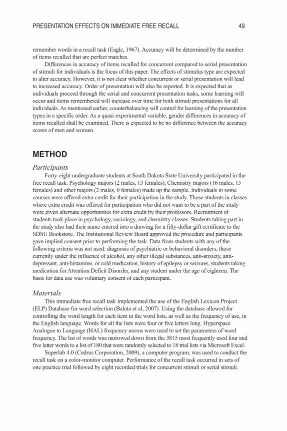
PRESENTATION EFFECTS ON IMMEDIATE FREE RECALL 49
remember words in a recall task (Eagle, 1967). Accuracy will be determined by the number
of items recalled that are perfect matches.
Differences in accuracy of items recalled for concurrent compared to serial presentation
of stimuli for individuals is the focus of this paper. The effects of stimulus type are expected
to alter accuracy. However, it is not clear whether concurrent or serial presentation will lead
to increased accuracy. Order of presentation will also be reported. It is expected that as
individuals proceed through the serial and concurrent presentation tasks, some learning will
occur and items remembered will increase over time for both stimuli presentations for all
individuals. As mentioned earlier, counterbalancing will control for learning of the presentation
types in a specific order. As a quasi-experimental variable, gender differences in accuracy of
items recalled shall be examined. There is expected to be no difference between the accuracy
scores of men and women.
METHOD
ParticipantsForty-eight undergraduate students at South Dakota State University participated in the
free recall task. Psychology majors (2 males, 13 females), Chemistry majors (16 males, 15
females) and other majors (2 males, 0 females) made up the sample. Individuals in some
courses were offered extra credit for their participation in the study. Those students in classes
where extra credit was offered for participation who did not want to be a part of the study
were given alternate opportunities for extra credit by their professors. Recruitment of
students took place in psychology, sociology, and chemistry classes. Students taking part in
the study also had their name entered into a drawing for a fifty-dollar gift certificate to the
SDSU Bookstore. The Institutional Review Board approved the procedure and participants
gave implied consent prior to performing the task. Data from students with any of the
following criteria was not used: diagnosis of psychiatric or behavioral disorders, those
currently under the influence of alcohol, any other illegal substances, anti-anxiety, anti-
depressant, anti-histamine, or cold medication, history of epilepsy or seizures, students taking
medication for Attention Deficit Disorder, and any student under the age of eighteen. The
basis for data use was voluntary consent of each participant.
MaterialsThis immediate free recall task implemented the use of the English Lexicon Project
(ELP) Database for word selection (Balota et al, 2007). Using the database allowed for
controlling the word length for each item in the word lists, as well as the frequency of use, in
the English language. Words for all the lists were four or five letters long. Hyperspace
Analogue to Language (HAL) frequency norms were used to set the parameters of word
frequency. The list of words was narrowed down from the 3815 most frequently used four and
five letter words to a list of 180 that were randomly selected to 18 trial lists via Microsoft Excel.
Superlab 4.0 (Cedrus Corporation, 2009), a computer program, was used to conduct the
recall task on a color-monitor computer. Performance of the recall task occurred in sets of
one practice trial followed by eight recorded trials for concurrent stimuli or serial stimuli.
GS019 JUR10_GS JUR text 1/11/11 11:41 AM Page 49

Whichever stimuli were presented for the first nine trials was then followed by a practice
trial and eight recorded trials of the other stimulus type. On the computer, serial presentation
occurred with a list of words one after the other. The single word appeared in the center of
the screen for two seconds and was immediately on the screen as the trial began. The second
word in the list, and all proceeding words, replaced the one before it after the two-second
time limit. There was no interval between words. At the end of the list of ten words, the
screen read “Begin Recall Now” and “Press 1 to End Recall.”
For concurrent presentation, the list of ten words appeared on the screen
simultaneously. In order to try to reduce chunking as much as possible, the words were
presented on separate lines and spread across the page. One word appeared on the first line,
and the second word was on the next line but across the page, with at least 14 spaces
between them. This process was used for each word, spanning the entire screen. As with the
serial presentation, the concurrent presentation appeared for two seconds per word, or for 20
seconds concurrently. After the 20 seconds, the “Begin Recall Now” screen appeared.
Participants used paper and a pencil to write down their responses for each recall task.
The paper was cut in half and each half-sheet of paper was stapled together into a packet
consisting of 16 half-sheets, eight each for the concurrent and serial lists. A demographic
survey at the end of the task obtained age, gender, and class standing for each participant.
Recorded answers were also printed using pencil and paper. The experimenters collected
data after the procedure period ended.
ProcedureThe recall task was conducted in a computer lab, on multiple days, with each session
supervised by one experimenter. Participants followed along as the experimenter read the
consent form. The final statement from the consent form stated that moving on with the
study would imply consent. Prior to the participants’ arrival, the computers were set up and
ready to run the recall task. Each stimulus presentation consisted of a practice trial and eight
trials of recorded recall. The experimenter read the directions for each task prior to running
through the practice and recorded trials. Each trial of serial lists contained ten words
presented one at a time. The first word appeared immediately after a command was entered
by the participant, and stayed on the screen for two seconds. Each word that followed
immediately appeared after two seconds. After ten words, the screen presenting “Begin
Recall Now” and “Press 1 to End Recall” flashed on the screen. This screen appeared for one
minute, unless the participant pressed the “1” key, in which case the screen would go blank.
After eight trials the directions for the concurrent presentation was read. The only
difference for the concurrent presentation consisted of all ten words presented simultaneously
for 20 seconds instead of one at a time for two seconds each. Again, the “Begin Recall Now”
screen prompted the participants to begin writing down the words for each trial. Participants
wrote their answers on a sheet of paper and flipped it over for each proceeding list.
Following the recall task, a demographic survey collected the age, gender, and class
standing of each participant. This survey, which was recorded using pencil and paper, also
had a question asking if consent was given to use the data for our study. Individuals could
respond “yes,” implying the data could be used, or “no,” implying their data could not be
used. Debriefing was included as well as informing the participants about the recall task and
5050 PRESENTATION EFFECTS ON IMMEDIATE FREE RECALL
GS019 JUR10_GS JUR text 1/11/11 11:41 AM Page 50

what it was intended to accomplish. Before and after the task, individuals were told they did
not need to participate.
ResultsFigure 1 shows the average (SD) number of correct responses to concurrent and serial
stimuli as a function of presentation order. For the individuals performing serial followed by
concurrent stimuli (Group 1), participants have an increased score on concurrent stimuli (M= 46.33, SD = 10.18). This is the largest mean for any stimulus type for either presentation
order. The average correct responses for concurrent stimuli, by the concurrent followed by
serial presentation participants (Group 2) is the lowest average score of accuracy (M = 41.17,
SD = 8.01). Serial stimuli for Group 1 (M = 44.04, SD = 9.83) and Group 2 (M = 43.17, SD =
8.10) are both relatively close and fall between the concurrent scores of each group.
As the current study is set to determine any differences in presentation order, stimulus type,
and gender, a two-way mixed ANOVA was calculated. The descriptive statistics for gender as
a function of presentation order and stimulus type are shown in Table 1. This data shows that
Group 1 men have the highest average number of correct responses to concurrent stimuli.
Group 1 men also have the largest average number of correct responses to serial stimuli.
However, Group 2 men have the lowest average scores to serial as well as concurrent stimuli,
when compared to Group 1 men and Group 1 and 2 women.
The two-way mixed ANOVA shows no main effect of the within factor of stimulus type
F (1/94) = .027, p = .871. Data for all interactions of significance, and error, for this ANOVA
are presented in Table 2, which shows the within-subjects factors, and Table 3, showing the
between subjects factors. Gender F (1/47) = .328, p = .57 and presentation order F (1/47) =
2.65, p = .111, the between subjects factors, also show no significant main effect. As Table 3
shows the stimulus type and presentation order interaction shows a significant effect at p =
.073, if significance level is at p < 0.1.
DiscussionAnalyzing the results of the mixed ANOVA showed no significant effect of stimulus
type, presentation order, gender, or any of their interactions. However, a medium effect was
found for the interaction of stimulus type by presentation order. The results showed that
participants in Group 1 and Group 2 both had increased scores as they moved from one
presentation type to the other, but not at a significant level. This finding leads to the possibility
that presentation of one stimuli followed by the other stimuli could allow for a learning
process in a temporal manner. This could allow individuals to have more responses that are
accurate in the second stimulus list. With a medium effect size it may be possible that if the
number of participants increased, a significant effect may be seen for the presentation order
and stimulus type interaction.
Looking at the results of the presentation order by stimulus type interaction, a greater
accuracy rate for Group 1 is possibly related to performing the serial presentation followed
by the concurrent presentation and learning the procedure. According to Cowan (2001), if
participants are allowed to see a list for a longer time, they are going to make larger chunks.
Since Group 1 saw the concurrent lists second in the presentation order, they may have
learned the procedure by performing the serial lists; and then performed better once doing
51PRESENTATION EFFECTS ON IMMEDIATE FREE RECALL 51
GS019 JUR10_GS JUR text 1/11/11 11:41 AM Page 51

the concurrent lists because it makes chunking more likely. Chunking has been found to
increase accuracy during recall (Eagle, 1967). Group 2 learned the procedure using the
concurrent list first; so they may not have performed as well as Group 1 on the second list,
which was serial for Group 2 individuals. If learning is what lead to an increase in the
average number of correct responses for both groups on the second set of stimulus lists, then
doing the concurrent list second may increase the number of correct responses at a higher
rate than performing the serial presentation second.
Bhatarah, Ward, Smith and Hayes (2009) found that faster presentation rates decreased
the accuracy of recall. The current study did not find a significant difference between
concurrent and serial presentation. However, presentation of the serial list, one word at a
time, prior to the concurrent stimuli lists, may allow the participants in Group 1 to have
increased accuracy on the concurrent lists. This may be due to learning the procedure and
then having a longer exposure to the concurrent list, which could increase the likelihood of
chunking (Cowan, 2001). Since both Group 1 and Group 2 had a slight increase in the
number of accurate responses on their second presentation, it is possible that learning of the
procedure may be likely. Counterbalancing the word lists and not just the presentation order
would be a benefit to future research. Then it would be possible to see if the second half of
the task had an increased number of words that could be recalled easier, or if learning is why
the participants performed better on the second set of presentations.
Gender differences for stimulus type and presentation order did not show any
significant effect either. However, men in Group 1 did have increased average accuracy
scores on both serial and concurrent lists, compared to men in Group 2, and women in both
groups. It was expected to find no significant difference in the average number of accurate
responses by men compared to women. Thus, this portion of the hypothesis is correct.
One important aspect to this study is that it found no significant difference between
individuals’ scores of accuracy for the two stimulus types. This might lead to more use of
concurrent stimuli in recall procedures. The lack of a significant difference between average
accuracy scores of individuals for each stimulus type does show that the two presentations
may use the same method of processing into long-term memory for words rehearsed when
the presentation began, and processing of recent words in working memory.
Comparing accuracy scores of concurrent and serial presentation does allow for
increased generalizability in the recall literature. There are few studies that have compared
the average correct responses to stimuli in a concurrent compared to a serial presentation.
Not one study was found that used ten words presented in each type as this one did. It is also
possible that a significant effect may have been found if close matches were counted as
correct responses along with the correctly spelled matches.
Further work on this procedure could make use of questioning the participants on what
strategy they used while the presentation of words occurred. If participants explained that
they used chunking or covert rehearsal, the data may explain learning strategies and the
differences in accuracy for each type. Chunking has been shown to increase accuracy scores
in comparison to rehearsal (Eagle, 1967). Otherwise, giving them directions that do not allow
a specific strategy could be implemented. Using articulatory suppression, a process of
making the participant repeatedly say a word, or words, during the presentation of stimuli,
could be used to control for chunking and rehearsal in both of these presentations (Russo &
52 PRESENTATION EFFECTS ON IMMEDIATE FREE RECALL
GS019 JUR10_GS JUR text 1/11/11 11:41 AM Page 52

Grammatopoulou, 2003). Also, delaying the recall portion of the task may show differences
in the accuracy of stimuli presentation. If participants are given time to rehearse the words
during a delay, between presentation and recall, it is possible that a difference in the encoding
of serial and concurrent stimuli would possibly show a difference in accuracy (Campoy, 2008).
This study had a large population of participants receiving extra credit. It may confound
results for the fact that only those people who need or want extra credit will participate.
Recruiting in three classes that did not offer extra credit resulted in zero participants. In order
to generalize the findings a population of students not receiving extra credit may be necessary.
The temperature in the lab where the procedure was performed was also variable. The heat
from no air-conditioning could cause changes in responses for the procedure. During the day,
the room had an increased temperature, especially on warm days. This may affect the accuracy
of responses as well. Further study of IFR and different presentation types is necessary.
REFERENCESAtkinson, R.C., & Shiffrin, R.M. (1968). Human memory: A proposed system and its control
processes. In Spence, K.W., Spence, J.T. (Eds.), The psychology of learning andmotivation: II (pp. 89-122). Oxford, England: Academic Press.
Balota, D.A., Yap, M.J., Cortese, M.J., Hutchison, K.A., Kessler, B., Loftis, B., … Treiman,
R. (2007) The English Lexicon Project. Behavior Research Methods, 39 (3), 445-459.
Baumeister, A.A., & Luszcz, M. (1976). A Within-subjects analysis of free recall with
preschool children. Child Development, 47, 729-736.
Bennett, I.J., Golob, E.J., Parker, E.S., & Starr, A. (2006). Memory evaluation in mild
cognitive impairment using recall and recognition tests. Journal of Clinical andExperimental Neuropsychology, 28, 1408-1422. doi: 10.1080/13803390500409583
Bhatarah, P., Ward, G., Smith, J., & Hayes, L. (2009). Examining the relationship between
free recall and immediate serial recall: Similar patterns of rehearsal and similar effects of
word length, presentation rate, and articulatory suppression. Memory & Cognition, 37,
689-713. doi: 10.3758/MC.37.5.689
Brbion, G., David, A.S., Bressan, R.A., & Pilowsky, L.S. (2006). Processing speed: a strong
predictor of verbal memory performance in schizophrenia. Journal of Clinical andExperimental Neuropsychology, 28, 370-382. doi: 10.1080/13803390590935390
Campoy, G. (2008). The effect of word length in short-term memory: is rehearsal necessary?.
The Quarterly Journal of Experimental Psychology, 61, 724-734. doi: 10.1080/
17470210701402364
Chen, Z. & Cowan, N. (2005). Chunk limits and length limits in immediate recall: A
reconciliation. Journal of Experimental Psychology: Learning, Memory, and Cognition,
31 (6), 1235-1249. doi: 10.1037/0278-7393.31.6.1235
Eagle, M.N. (1967). The effect of learning strategies on free recall. The American Journal ofPsychology, 80(3), 421-425. doi: 10.23071420376
Gazzaniga, M.S., Ivry, R.B., & Mangun, G.R. (2009). Learning and memory. In Durbin, J.W.
(Ed.) Cognitive neuroscience: The biology of the mind (312-363).New York: W.W.
Norton & Company, Inc.
Haist, F., Shimamura, A.P., & Squire, L.R. (1992). On the relationship between recall and
PRESENTATION EFFECTS ON IMMEDIATE FREE RECALL 53
GS019 JUR10_GS JUR text 1/11/11 11:41 AM Page 53

54 PRESENTATION EFFECTS ON IMMEDIATE FREE RECALL
recognition memory. Journal of Experimental Psychology: Learning, Memory andCognition, 18(4), 691-702.
Harness, A., Jacot, L., Scherf, S., White, A., & Warnick, J.E. (2008). Sex differences in
working memory. Psychological Reports, 103(1), 214-218. Abstract retrieved from
http://search.ebscohost.com.
Hoppe, C., Stojanovic, J., Karg Foundation Young Researchers Group 2008/09, Elger, C.E.
(2009). Enhancing memory for lists by grouped presentation and rehearsal: A pilot study
in healthy subjects with unexpected results. Seizure, 18, 711-715. doi:
10.1016/j.seizure2009.10.001
Huang, I., Tomasini, J., & Nikl, L. (1977). The primacy and recency effects in successive
single-trial immediate free recall. The Journal of General Psychology, 97, 157-165.
Jelinek, L., Jacobsen, D., Kellner, M., Larbig, F., Biesold, K.-H., Barre, K., Moritz, S. (2006)
Verbal and nonverbal memory functioning in posttraumatic stress disorder (PTSD).
Journal of Clinical and Experimental Neuropsychology, 28, 940-948. doi:
10.1080/13803390591004347
Joseph, C.A., McKay, T.D., & Joseph, C.R. (1982). Sex effects on free recall of transforming
orally and visually presented nouns into printed, picture, or imagery form. The Journal ofGeneral Psychology, 107, 51-55.
Laming, D. (2009). Failure to recall. Psychological Review, 116(1), 157-186. Abstract
retrieved from http://apps.isiknowledge.com.
Matlin, M. W. (1976). The relationship between english word length and short-term memory.
The Journal of General Psychology, 94, 47-57.
McDowell, B.D., Bayless, J.D., Moser, D.J., Meyers, J.E., & Paulsen, J.S. (2004).
Concordance between the CVLT and the WMS-iii word lists test. Archives of ClinicalNeuropsychology, 19, 319-324. doi:10.1016/S0887-6177(03)00023-4
Microsoft Excel® 2007 [Computer Software] (2010) Microsoft Corporation.
Miller, G.A. (1956). The magical number seven, plus or minus two some limits on our
capacity for processing information. Psychological Review, 101 (2), 343-352.
Ozubko, J.D., & Joordens, S. (2007). The mixed truth about frequency effects on free recall:
effects of study list composition. Psychonomic Bulletin & Review, 14(5), 871-876.
Russo, R., & Grammatopoulou, N. (2003). Word length and articulatory suppression affect
short-term and long-term recall tasks. Memory & Cognition, 31(5), 728-737.
Seiler, K.H., & Engelkamp, J. (2003). The role of item-specific information for serial
position curve in free recall. Journal of Experimental Psychology: Learning, Memory &Cognition, 29, 954-964. doi: 10.1037/0278-7393.29.5.954
Smith, A.P., Jones, D.M., & Broadbent, D.E. (1981). The effects of noise on recall of
categorized lists. British Journal of Psychology, 72, 299-316.
Sneed, P.R., Brunts, D.C., & Mueller, J.H. (1977). Instructions and grouped presentation in
free recall. American Journal of Psychology, 90(2), 263-268.
SuperLab (Version 4.0) [Computer Software] (2009) San Pedro, CA; Cedrus Corporation
Ward, G., & Maylor, E.A. (2005). Age-related deficits in free recall: the role of rehearsal.
The Quarterly Journal of Experimental Psychology, 58A, 98-119. doi:
10.1080/02724980443000223
Ward, G., & Tan, L. (2004). The effect of the length of to-be-remembered lists and
GS019 JUR10_GS JUR text 1/11/11 11:41 AM Page 54

intervening lists on free recall: a reexamination using overt rehearsal. Journal ofExperimental Psychology: Learning, Memory and Cognition, 30, 1196-1210. doi:
10.1037/0278-7393.30.6.1196
Table 1: Average (SD) Number of Correct Responses to Serial and Concurrent Stimuli as aFunction of Gender and Presentation Order
Men Women
Stimulus Serial Then Concurrent Serial Then ConcurrentType Concurrent Then Serial Total Concurrent Then Serial Total
Serial 47.86 42.23 44.20 42.47 44.27 43.18
(8.36) (8.36) (8.73) (10.18) (7.72) (9.18)
Concurrent 50.29 39.69 43.40 44.71 42.91 44.00
(11.57) (8.38) (17.73) (9.43) (7.57) (8.65)
Table 2: ANOVA Tests of Within-Subjects Factors and Effect Size
Sum of Mean Partial EtaSource Squares df Square F Sig. Squared
Stimulus Type .785 1 .785 .027 .871 .001
Stimulus Type 99.287 1 99.287 3.370 .073 .071
by Order
Stimulus Type 1.304 1 1.304 .044 .834 .001
by Gender
Stimulus Type by 2.533 1 2.533 .086 .771 .002Order by Gender
Error (Stimulus Type) 1296.275 44 29.461
Table 3: ANOVA Tests of Between-Subjects Factors and Effect Size
Sum of Partial EtaSource Squares df Mean Square F Sig. Squared
Order 355.749 1 355.749 2.650 .111 .057
Gender 44.081 1 44.081 .328 .570 .007
Order by Gender 356.219 1 356.219 2.654 .110 .057
Error 5905.944 44 134.226
PRESENTATION EFFECTS ON IMMEDIATE FREE RECALL 55
GS019 JUR10_GS JUR text 1/11/11 11:41 AM Page 55

56 PRESENTATION EFFECTS ON IMMEDIATE FREE RECALL
Figure 1. Average accurate responses to serial and concurrent stimuli as a function of
presentation order. Error bars represent standard deviation.
GS019 JUR10_GS JUR text 1/11/11 11:41 AM Page 56
The Effects of Feedback on StudentPerformance While Performing MultipleTasks Simultaneously
Authors: Amber Reis, Danyel JanssenFaculty Advisor: Dr. Deborah SpearDepartment: Psychology
ABSTRACTResearch shows that feedback or knowledge of results can increase performance on
multiple activities. In order for feedback to be successful, it should follow closely in time to
the behavior. The current study is a between-group design where the experimental group
received visual feedback in the form of a point total about their accuracy in performing a
computer task and the control group was not presented with the point totals. While the
experimental group did have higher average point totals, the results were not statistically
significant. Gender served as the second independent variable and there was not a significant
difference between the average total points for men and women. There was not a significant
interaction between the two variables.
THE EFFECTS OF FEEDBACK ON STUDENTPERFORMANCE WHILE PERFORMING MULTIPLE TASKSSIMULTANEOUSLY
Knowledge of results (KR) is “feedback containing the level of performance obtained”
(“Feedback,” 2000, p.172). Several studies have investigated the effect of knowledge of
results on the performance of different tasks. Information about how knowledge of results
can influence performance is beneficial for the fields of education and behavior
modification. Some educational facilities are currently putting this scientific information into
practice. Pokorny and Pickford (2010) researched student perceptions of feedback on
academic performance and found that lengthy written feedback is not affective in response to
a final paper or project. Students reported that an instructor’s feedback is most beneficial
when followed closely behind the assignment.
Several populations have been used to study the effects of knowledge of results or
feedback. Individuals with either physical or mental handicaps are often the subjects of
feedback studies, one study by Hemayattalab and Rostami (2010) examined the effects of
knowledge of results in dart throwing abilities of children with cerebral palsy. They used an
ANOVA to test their results and found that those in the feedback condition were able to learn
new motor tasks. In a study conducted by Carroll (1973), normal male participants ages 18 to
29 completed different perceptual-motor tasks with and without performance feedback. The
EFFECTS OF FEEDBACK 57
GS019 JUR10_GS JUR text 1/11/11 11:41 AM Page 57
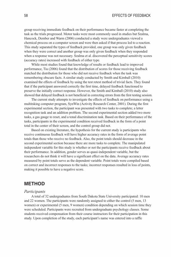
group receiving immediate feedback on their performance became faster at completing the
task as the trials progressed. Motor tasks were most commonly used in studies but Szalma,
Hancock, Dember and Warm (2006) conducted a study were undergraduates viewed a
chemical process on a computer screen and were then asked if that process led to a reaction.
This study separated the types of feedback provided, one group was only given feedback
when they were correct and another group was only given feedback when they responded
when a response was not necessary. Szalma et al. discovered the perceptual sensitivity scores
(accuracy rates) increased with feedback of either type.
While most studies found that knowledge of results or feedback lead to improved
performance, Tiu (2006) found that the distribution of scores for those receiving feedback
matched the distribution for those who did not receive feedback when the task was
remembering obscure facts. A similar study conducted by Smith and Kimball (2010)
examined the effects of feedback by using the test retest method of trivial facts. They found
that if the participant answered correctly the first time, delayed feedback functioned to
preserve the initially correct response. However, the Smith and Kimball (2010) study also
showed that delayed feedback is not beneficial in correcting errors from the first testing session.
The current study attempts to investigate the effects of feedback on performance using a
multitsking computer program, SynWin (Activity Research Center, 2001). During the first
experimental section, the participant was presented with two tasks to complete; a letter
recognition task and an addition problem. The second experimental section added two more
tasks, a gas gauge to reset, and a tonal discrimination task. Based on their performance of the
tasks, participants in the experimental condition received feedback in the form of a point
total in the center of their screen, and the control group did not.
Based on existing literature, the hypothesis for the current study is participants who
receive continuous feedback will have higher accuracy rates in the form of average point
totals than those who receive no feedback. Also, the point totals should decrease in the
second experimental section because there are more tasks to complete. The manipulated
independent variable for this study is whether or not the participants receive feedback about
their performance. In addition, gender serves as quasi-independent variable, but the
researchers do not think it will have a significant effect on the data. Average accuracy rates
measured by point totals serve as the dependent variable. Point totals were compiled based
on correct and incorrect responses to the tasks; incorrect responses resulted in loss of points,
making it possible to have a negative score.
METHOD
ParticipantsA total of 32 undergraduates from South Dakota State University participated: 10 men
and 22 women. The participants were randomly assigned to either the control (5 men, 13
women) or experimental (5 men, 9 women) condition depending on which session time they
were scheduled. Participants were recruited from undergraduate psychology classes. Some
students received compensation from their course instructors for their participation in this
study. Upon completion of the study, each participant’s name was entered into a raffle
58 EFFECTS OF FEEDBACK
GS019 JUR10_GS JUR text 1/11/11 11:41 AM Page 58

drawing with the chance to win a coupon or gift card to Cubby’s Sports Bar and Grill, SDSU
Dairy Bar, and Brookings Cinema 5. Students with a current diagnosis of any form of
psychiatric or behavioral disorder, students under the influence of alcohol, illegal substances,
any antidepressant or anti-anxiety drug or cold medicine, students with a history of epilepsy
or seizures, students taking any medication for Attention Deficit Disorder, and students under
the age of eighteen did not have their results included in the final data analysis. The
Institutional Review Board approved the current study.
MaterialsComputers were used to show the participants the SynWin (Activity Research Center,
2001) program containing the experiment. The program recorded responses to all the tasks in
addition to the total points for both conditions. The demographic information sheet served as
an implied consent form that the participants completed and returned.
ProceduresBoth groups performed the same tasks under the same environmental conditions; the
only difference was the experimental group was provided with visual feedback in the form of
a score in the middle of their screen. This score provided the participants with continuous
visual feedback about their accuracy in completing the tasks.
The information sheet was read aloud and the participants were told that their consent
was implied by their completion and submission of their demographic information sheet. A
short demographic information sheet containing questions about the participant’s age, major,
and gender, was then completed and sealed in individual manila envelopes. The participants
were given three minutes to practice and become familiar with the SynWin program and the
tasks to be completed. In the upper left corner was a letter recognition task, and the upper
right corner had the math problem, as seen in Figure 1. Immediately following the practice,
the participants began the 15-minute experimental session with only the two tasks. The
second part of the experiment followed the same pattern as the first part, but included two
additional tasks. The lower left corner had a gauge that needed to be reset and the lower right
corner had an alert circle to be clicked when the participant heard a high tone from a
background of low tones. During the tasks, the experimental group received visual feedback
in the form of point totals. Once all participants finished the second 15-minute experimental
part, they were debriefed as to the hypothesis of the study
RESULTSThe average total points are presented in figures 2 and 3 for each of the independent
variables. Figure 2 examines the average point totals between the no feedback and feedback
conditions. The experimental group has a higher total point average than the control group,
but there is large variation between the two groups (M=3059.79, SD= 1220.91; M=2050,
SD=1515.548435 respectively). A two-way between ANOVA using experimental condition
and gender as the two variables, shows there is no significant main effect of experimental
condition on average point totals [F(1,28)=1.877, p=.182].
EFFECTS OF FEEDBACK 59
GS019 JUR10_GS JUR text 1/11/11 11:41 AM Page 59
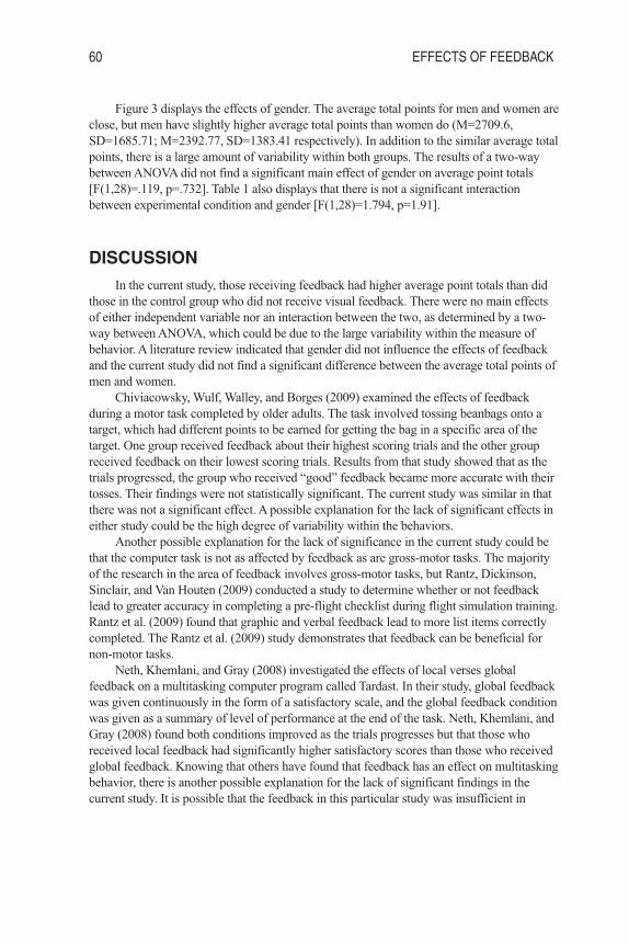
Figure 3 displays the effects of gender. The average total points for men and women are
close, but men have slightly higher average total points than women do (M=2709.6,
SD=1685.71; M=2392.77, SD=1383.41 respectively). In addition to the similar average total
points, there is a large amount of variability within both groups. The results of a two-way
between ANOVA did not find a significant main effect of gender on average point totals
[F(1,28)=.119, p=.732]. Table 1 also displays that there is not a significant interaction
between experimental condition and gender [F(1,28)=1.794, p=1.91].
DISCUSSIONIn the current study, those receiving feedback had higher average point totals than did
those in the control group who did not receive visual feedback. There were no main effects
of either independent variable nor an interaction between the two, as determined by a two-
way between ANOVA, which could be due to the large variability within the measure of
behavior. A literature review indicated that gender did not influence the effects of feedback
and the current study did not find a significant difference between the average total points of
men and women.
Chiviacowsky, Wulf, Walley, and Borges (2009) examined the effects of feedback
during a motor task completed by older adults. The task involved tossing beanbags onto a
target, which had different points to be earned for getting the bag in a specific area of the
target. One group received feedback about their highest scoring trials and the other group
received feedback on their lowest scoring trials. Results from that study showed that as the
trials progressed, the group who received “good” feedback became more accurate with their
tosses. Their findings were not statistically significant. The current study was similar in that
there was not a significant effect. A possible explanation for the lack of significant effects in
either study could be the high degree of variability within the behaviors.
Another possible explanation for the lack of significance in the current study could be
that the computer task is not as affected by feedback as are gross-motor tasks. The majority
of the research in the area of feedback involves gross-motor tasks, but Rantz, Dickinson,
Sinclair, and Van Houten (2009) conducted a study to determine whether or not feedback
lead to greater accuracy in completing a pre-flight checklist during flight simulation training.
Rantz et al. (2009) found that graphic and verbal feedback lead to more list items correctly
completed. The Rantz et al. (2009) study demonstrates that feedback can be beneficial for
non-motor tasks.
Neth, Khemlani, and Gray (2008) investigated the effects of local verses global
feedback on a multitasking computer program called Tardast. In their study, global feedback
was given continuously in the form of a satisfactory scale, and the global feedback condition
was given as a summary of level of performance at the end of the task. Neth, Khemlani, and
Gray (2008) found both conditions improved as the trials progresses but that those who
received local feedback had significantly higher satisfactory scores than those who received
global feedback. Knowing that others have found that feedback has an effect on multitasking
behavior, there is another possible explanation for the lack of significant findings in the
current study. It is possible that the feedback in this particular study was insufficient in
60 EFFECTS OF FEEDBACK
GS019 JUR10_GS JUR text 1/11/11 11:41 AM Page 60
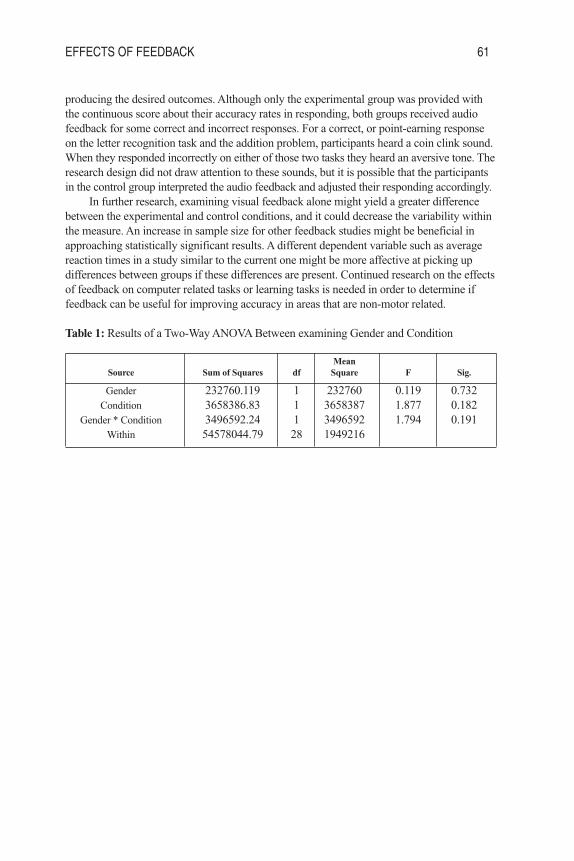
producing the desired outcomes. Although only the experimental group was provided with
the continuous score about their accuracy rates in responding, both groups received audio
feedback for some correct and incorrect responses. For a correct, or point-earning response
on the letter recognition task and the addition problem, participants heard a coin clink sound.
When they responded incorrectly on either of those two tasks they heard an aversive tone. The
research design did not draw attention to these sounds, but it is possible that the participants
in the control group interpreted the audio feedback and adjusted their responding accordingly.
In further research, examining visual feedback alone might yield a greater difference
between the experimental and control conditions, and it could decrease the variability within
the measure. An increase in sample size for other feedback studies might be beneficial in
approaching statistically significant results. A different dependent variable such as average
reaction times in a study similar to the current one might be more affective at picking up
differences between groups if these differences are present. Continued research on the effects
of feedback on computer related tasks or learning tasks is needed in order to determine if
feedback can be useful for improving accuracy in areas that are non-motor related.
Table 1: Results of a Two-Way ANOVA Between examining Gender and Condition
MeanSource Sum of Squares df Square F Sig.
Gender 232760.119 1 232760 0.119 0.732
Condition 3658386.83 1 3658387 1.877 0.182
Gender * Condition 3496592.24 1 3496592 1.794 0.191
Within 54578044.79 28 1949216
EFFECTS OF FEEDBACK 61
GS019 JUR10_GS JUR text 1/11/11 11:41 AM Page 61

Figure 1. A screen shot of the SynWin program for the experimental condition is shown.
Figure 2. The average total points for the experimental and control conditions. Error bars
represent the standard deviation.
62 EFFECTS OF FEEDBACK
GS019 JUR10_GS JUR text 1/11/11 11:41 AM Page 62

Figure 3. The average total points for men and women. Error bars represent the standard
deviation.
REFERENCESCarroll, E.A. (1973). The effects of knowledge of results and level of aspiration upon the
learning and retention of a psycho-motor task. (Masters Thesis) Available from
http://etd.lib.ttu.edu/theses/available/etd-07242009-31295015505810/unrestricted/
31295015505810.pdf
Chiviacowsky, S., Wulf, G., Walley,R., and Borges, T. (2009) Knowledge of results after
good trials enhances learning in older adults. Research Quarterly for Exercise & Sport, 80(3) 663-668.
Feedback and knowledge of results. (2000). In Matthews, G., Davies, D.R., Westerman, S.J.,
& Stammers, R.B. (Eds.), Human performance: Cognition, stress and individual
differences. Philadelphia: Psychology Press.
Hemayattalab, R., & Rostami, L.R. (2010) Effects of frequency of feedback on the learning
of motor skills in individuals with cerebral palsy. Research in Developmental Disabilities,31 (1) 212-217. Abstract retrieved from Ebscohost.
Neth, H., Khemlain, S.S., & Gray, W.D. (2008) Feedback design for the control of a dynamic
multitasking system: Dissociating outcome feedback from control feedback. HumanFactors, 50 (4) 643-651.
Pokorny, K. & Pickford, P. (2010). Complexity, cues and relationships: Student perceptions
of feedback. Active Learning in Higher Education, 11 (1) 21-30.
Smith, T.A. & Kimball, D.R. (2010). Learning from feedback: Spacing and the
delay–retention effect. Journal of Experimental Psychology: Learning, Memory, andCognition, 36 (1), 80-95.
SynWin (Version 1.2.28) [Computer Software.] Chula Vista, California: Activity
Research Services.
Szalma, J.L., Hancock, P.A., Dember, W.N., & Warm, J.S. (2006) Training for vigilance: The
effect of knowledge of results format and dispositional optimism and pessimism on
performance and stress. British Journal of Psychology, 97, 115-135.
EFFECTS OF FEEDBACK 63
GS019 JUR10_GS JUR text 1/11/11 11:41 AM Page 63

Tiu, J.H. (2006) The effect of knowledge of results on motivation and performance.
Dissertation Abstracts International: Section B: The Sciences and Engineering, 67 (5-B),
2880. Abstract retrieved from Ebscohost.
Rantz, W.G., Dickinson, A.M., Sinclair, G.A., & Van Houten, R. (2009) The effect of
feedback on the accuracy of checklist completion during instrumental flight training.
Journal of Applied Behavior Analysis, 42, 497-510.
64 EFFECTS OF FEEDBACK
GS019 JUR10_GS JUR text 1/11/11 11:41 AM Page 64

TRACKING BARE SAND MOBILIZATION FROM LANDSCAPE MANIPULATIONS 65
Tracking Bare Sand Mobilization Arisingfrom Landscape Manipulations in theGrasslands Destabilization Experiment(GDEX) in the Nebraska Sandhills UsingImaging Spectroscopy
Author: Benjamin Helder, B.S.Faculty Sponsor: Geoffrey M. Henebry, Ph.D., C.S.E.Department: Geography; Geographic Information Science
Center of Excellence (GIScCE)
ABSTRACTThe Grassland Destabilization Experiment (GDEX) is a landscape scale manipulative
experiment initiated in 2004 in the Nebraska Sandhills to evaluate changes in surface
properties following the abrupt loss of stabilizing vegetation.
The GDEX features five treatments allocated among ten plots of 120 m in diameter
(1.13 ha). The Aggressive Bare Sand protocol included chemical defoliation and subsequent
shallow disking and raking in 2004 to devegetate the plot with periodic physical disturbance
to maintain bare sand. The Long Term Disturbance (Press) protocol includes an initial chemical
defoliation in May 2005 and seasonal spring reapplications, but no physical disturbance.
Short Term Disturbance (Pulse) treatment had chemical defoliation initially in 2005 and
again in 2008; thus, 2006, 2007, and 2009 are “recovery” years. There are two sets of
controls: Grazed and Ungrazed. Eight plots (two replicates of each treatment) located
contiguously within a fence are the focus of our investigation: Ungrazed Control, Pulse,
Press, and Bare Sand. (We excluded the two Grazed Control plots that were located outside
the fence away from the other treatments.)
Erosion pin networks were established in each plot to track net (gain-loss) sand
movement. Remote sensing data were acquired using the AISA Eagle imaging spectrometer
in late June from 2006 through 2009. We tracked the spread of bare sand within and outside of
the treatment plots by thresholding the upper range of values in the green (517 nm), red (666
nm), red edge (713 nm), and near infrared (856 nm) portions of the electromagnetic spectrum.
The average reflectance across the full spectral range of the imagery (396-980 nm) at
the erosion pin locations increased in the Press and Bare Sand treatments from 0.25 in 2006
to 0.30 in 2009; it decreased over the same period in Pulse treatments from 0.19 to 0.17 and
in Ungrazed Controls from 0.17 to 0.14. Increases in the areal extent of bare sand in the
neighborhood of the plots between 2006 and 2009 were an average of 5,742 m2 for Presstreatments and 713 m2 for Bare Sand treatments. Four years elapsed before sustained sand
mobilization occurred. We expect sand in the Bare Sand and Press treatments to continue to
move as long as experimental treatments are maintained.
GS019 JUR10_GS JUR text 1/11/11 11:41 AM Page 65
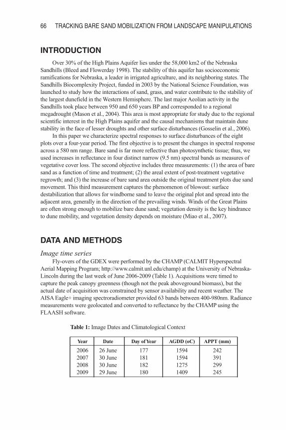
66 TRACKING BARE SAND MOBILIZATION FROM LANDSCAPE MANIPULATIONS
INTRODUCTIONOver 30% of the High Plains Aquifer lies under the 58,000 km2 of the Nebraska
Sandhills (Bleed and Flowerday 1998). The stability of this aquifer has socioeconomic
ramifications for Nebraska, a leader in irrigated agriculture, and its neighboring states. The
Sandhills Biocomplexity Project, funded in 2003 by the National Science Foundation, was
launched to study how the interactions of sand, grass, and water contribute to the stability of
the largest dunefield in the Western Hemisphere. The last major Aeolian activity in the
Sandhills took place between 950 and 650 years BP and corresponded to a regional
megadrought (Mason et al., 2004). This area is most appropriate for study due to the regional
scientific interest in the High Plains aquifer and the causal mechanisms that maintain dune
stability in the face of lesser droughts and other surface disturbances (Gosselin et al., 2006).
In this paper we characterize spectral responses to surface disturbances of the eight
plots over a four-year period. The first objective is to present the changes in spectral response
across a 580 nm range. Bare sand is far more reflective than photosynthetic tissue; thus, we
used increases in reflectance in four distinct narrow (9.5 nm) spectral bands as measures of
vegetative cover loss. The second objective includes three measurements: (1) the area of bare
sand as a function of time and treatment; (2) the areal extent of post-treatment vegetative
regrowth; and (3) the increase of bare sand area outside the original treatment plots due sand
movement. This third measurement captures the phenomenon of blowout: surface
destabilization that allows for windborne sand to leave the original plot and spread into the
adjacent area, generally in the direction of the prevailing winds. Winds of the Great Plains
are often strong enough to mobilize bare dune sand; vegetation density is the key hindrance
to dune mobility, and vegetation density depends on moisture (Miao et al., 2007).
DATA AND METHODS
Image time seriesFly-overs of the GDEX were performed by the CHAMP (CALMIT Hyperspectral
Aerial Mapping Program; http://www.calmit.unl.edu/champ) at the University of Nebraska-
Lincoln during the last week of June 2006-2009 (Table 1). Acquisitions were timed to
capture the peak canopy greenness (though not the peak aboveground biomass), but the
actual date of acquisition was constrained by sensor availability and recent weather. The
AISA Eagle+ imaging spectroradiometer provided 63 bands between 400-980nm. Radiance
measurements were geolocated and converted to reflectance by the CHAMP using the
FLAASH software.
Table 1: Image Dates and Climatological Context
Year Date Day of Year AGDD (oC) APPT (mm)
2006 26 June 177 1594 242
2007 30 June 181 1594 391
2008 30 June 182 1275 299
2009 29 June 180 1409 245
GS019 JUR10_GS JUR text 1/11/11 11:41 AM Page 66

TRACKING BARE SAND MOBILIZATION FROM LANDSCAPE MANIPULATIONS 67
Monitoring sitesErosion pin networks had been established by other GDEX researchers to track net
(gain-loss) sand movement. A geolocated network was established within each treatment plot
for a total of 364 graduated pieces of aluminum conduit emplaced across the eight plots. We
used these locations to monitor variations in surface reflectance over the four-year period,
but we did not analyze here the corresponding erosion data.
Meteorological dataDaily precipitation and temperature data were obtained for the Barta Brothers Ranch
automated station maintained by the High Plains Regional Climate Center (hprcc.unl.edu).
We calculated accumulated growing degree days (AGDD) from 01 January of each year
using a base temperature of 0 oC (=273.15 K) following de Beurs and Henebry (2004). We
calculated the accumulated precipitation as the running sum of daily precipitation.
Masking high reflectanceWe identified areas of bare sand within and adjacent to the treatment plots by masking
out those data that fell below a critical threshold. Due to interannual climatic variability
(Table 1), we chose the optimal threshold for each band for each year rather than selecting a
general threshold across years. Masks were generated at four wavelengths, each representing
a narrow slice of the electromagnetic spectrum useful for vegetation analysis: green (517
nm), red (666 nm), red edge (713 nm), near infrared or NIR (856 nm). Reflectance from
healthy vegetation in the visible wavelengths (400-680 nm) is generally highest in green and
lowest in red. Red light is strongly absorbed by green vegetation for use in photosynthesis,
but strongly reflected by bare sand; thus, a temporal trend of increasing red reflectance
indicates decreasing vegetative cover. The red edge in vegetation spectra spans roughly 700-
720nm covering the transition from the low reflectance/high absorption of the red to the high
reflectance/low absorption of the NIR. Measurements in this transition are good indicators of
photosynthetic activity and overall vegetation health (Gitelson et al., 1995). NIR covers
approximately 750-1000nm and is useful for distinguishing healthy from distressed vegetation.
Using the ENVI package (v4.6; ITTVIS 2009), we contrasted the boundaries of original
120m diameter plots as blue against the black and white mask images. This technique
allowed us to discern at a glance the original plots outlined in color, bare sand in white, and
vegetated areas in black (Figure 1). ENVI’s Region of Interest (ROI) tool was then used to
determine the number of white (bare sand) pixels and thus the areal extent of bare sand. We
also determined area of blowouts, where the bare sand has mobilized and been deposited
beyond the extent of the original plot. Overall area can differ from original size plus blowout;
some plots show regrowth depending on treatment type.
GS019 JUR10_GS JUR text 1/11/11 11:41 AM Page 67

Figure 1. High reflectance mask in green (513-522 nm) for 2009. Numbers indicate plot
designations: Press treatment in 1 & 8; Bare Sand in 5 & 7.
RESULTS
Spectral Response ChangesThe average Green reflectance at erosion pin locations increased in Press and Bare
Sand treatments by 0.05 between 2006 and 2009, while Pulse and Ungrazed Control plots
decreased 0.02 (Figure 2A). For Red, Press and Bare Sand showed an increase of 0.09, while
Pulse and Ungrazed Control decreased 0.04 (Figure 2B). For Red Edge, Press and BareSand plots increased 0.08, while Pulse and Ungrazed Control decreased 0.02 (Figure 2C).
The average NIR reflectance in Press and Bare Sand plots increased by 0.06, but Pulseand Ungrazed Control remained constant (Figure 2D). Analysis of the entire spectral range
showed a reflectance value of 0.25 in 2006 increasing to 0.30 in 2009 in Press and BareSand plots. It decreased over the same period in Pulse and Ungrazed Control treatments by
0.03 (Figure 3).
Note the decrease in reflectance in 2007 that is consistent across treatments (Figure 3).
This decrease reflectance indicates increased vegetative cover, which is attributed to plentiful
precipitation (391 mm in 2007 vs. the 289 mm average for 30 June for 2000-2009).
68 TRACKING BARE SAND MOBILIZATION FROM LANDSCAPE MANIPULATIONS
GS019 JUR10_GS JUR text 1/11/11 11:41 AM Page 68

Figure 2: Average plot reflectance by band: (A) Green (513–522 nm); (B) Red (671–680
nm); (C) Red Edge (709–718 nm); (D) NIR (852–861 nm).
TRACKING BARE SAND MOBILIZATION FROM LANDSCAPE MANIPULATIONS 69
GS019 JUR10_GS JUR text 1/11/11 11:41 AM Page 69

Figure 3. Average plot reflectance ordered by intensity. The hierarchical x-axis displays
year of acquisition (200x), plot designation, and plot treatment.
Areal ChangesThe original area of each treatment plot as established in 2004 was 11,300 m2. Table 2
shows bare sand area detected by all four bands in 2009. Pulse and Ungrazed Control plots
exhibited no bare sand area in all four bands in 2009. Total area of Press plots decreased at
an average of 4,298 m2 per plot; whereas, the exposed area of Bare Sand plots increased by
an average of 623 m2.
Table 2: Total Bare Sand Area in 2009
Plot & Treatment Bare Sand Area (m2)
1 (Press) 7,056
5 (Bare Sand) 12,004
7 (Bare Sand) 11,842
8 (Press) 6,948
Plots 5 and 7 (both Bare Sand treatments) were the only plots to feature blowout detected
in all four bands, totaling 2,527 m2 and 1,814 m2 respectively. No identifiable blowouts
were evident in Pulse or Ungrazed Control plots. Rather, the Pulse plots were almost entirely
revegetated and the Ungrazed Control plots never exhibited bare sand patches.
70 TRACKING BARE SAND MOBILIZATION FROM LANDSCAPE MANIPULATIONS
GS019 JUR10_GS JUR text 1/11/11 11:41 AM Page 70

The occurrence of blowout depended on treatment and site history. Plot 5 (Bare Sandtreatment), which was constructed on an existing blowout, showed sand movement before
four years had elapsed. In contrast, Plot 7 (also Bare Sand treatment) showed little
movement before the fourth year. Plots 1 and 8, both Press treatments also showed divergent
blowout results, perhaps due to local terrain differences. In each spectral subset, Plot 8
showed roughly four times the blowout area of Plot 1.
Figure 4: Changes in bare sand area and blowout area: (A) Green (513 – 522nm); (B) Red
(671 – 680nm); (C) Red Edge (709 – 718nm); and (D) NIR (852 – 861nm). Solid lines
indicate bare sand area and dashed lines indicate area of blowout. Dashed tan line shows
original 11300 m2 plot size in 2004.
DISCUSSION & CONCLUSIONPlot reflectance relates to plot treatment; the differences being most prevalently
exhibited by results in NIR. Bare Sand plots demonstrate divergence in reflectance through
2008 followed by convergence in 2009. In nearly all bands/years, plot order of reflectance
remained constant, Bare Sand and Press plots ordering first and second. Peculiar is the
TRACKING BARE SAND MOBILIZATION FROM LANDSCAPE MANIPULATIONS 71
GS019 JUR10_GS JUR text 1/11/11 11:41 AM Page 71

behavior of Pulse plots reflectances in the NIR band in 2009. After having reflectance lower
than even the Control plots in 2008, in 2009 the Pulse plots pass the Control plots and
produce reflectance values closer to those of Press and Bare Sand plots in any other
band/year combination. All bands show decreased reflectance in 2007. This may result from
above average rainfall. Press and Bare Sand values were nearly identical, as were those of
Pulse and Control plots. It is unclear if the high precipitation that caused lower reflectances
in 2007 had a similar effect on 2008 data or whether it was due to lower evapotranspiration
caused by a cooler spring (Table 1). Another possible explanation is differences in the AISA
sensor setup or processing.
Press plots (repeated herbicide applications but no physical disturbance) exhibit the
sharpest gains in overall area, yet show substantial revegetation beginning in 2008 with no
increase in 2009. Bare Sand plots (initial herbicide plus periodic disking and raking) tended
to vary less but did not regain the same area or blowout values after the wet year of 2007
until 2009. All plots showed areal decreases in 2008 in the red, red edge, and NIR bands.
However, all plots in the green band showed areal increase. This is explained by the presence
of prairie grass, which reflects relatively more in the green wavelengths than it does in red,
red edge or NIR.
Overall plot area in 2007 generally decreased for Bare Sand plots while it increased for
Press plots. This trend also holds true for corresponding blowout values. Increased moisture
was unable to impact the original plot areas but did substantially reduce blowout, leading to
lower total area values for Bare Sand plots, which feature more blowout area.
Another AISA Eagle+ acquisition is schedule for June 2010. However, there has been a
change in the GDEX protocol. Plots 5 and 7, formerly Bare Sand treatments are being
purposely revegetated to study the stabilization process. During the first half of 2010 Plot 7 is
being planted with woody vegetation while Plot 5 is being seeded with grasses and forbs.
Thus, as the GDEX morphs into GREX, we will be able to track the progress of the
restabilization using the techniques described above.
ACKNOWLEDGEMENTSWe thank Dr. Dave Wedin, the GDEX PI, for helpful comments on an earlier draft.
This research was supported in part by the NASA EPSCoR program and the GIScCE Center
Scholars Program at SDSU. Meteorological data for Barta Brothers Ranch was obtained
through the High Plains Regional Climate Center. GDEX implementation and image
acquisitions were made possible through support from the National Science Foundation’s
Biocomplexity Program.
REFERENCESBleed AS, Flowerday CA. 1998. An Atlas of the Sand Hills. The University of Nebraska
Press: Lincoln, NE. 260 pp.
72 TRACKING BARE SAND MOBILIZATION FROM LANDSCAPE MANIPULATIONS
GS019 JUR10_GS JUR text 1/11/11 11:41 AM Page 72

de Beurs KM, Henebry GM. 2004. Land surface phenology, climatic variation, and
institutional change: Analyzing agricultural land cover change in Kazakhstan. RemoteSensing of Environment 89: 497-509.
Gitelson AA, Merzlyak MN, Lichtenthaler HK. 1995. Detection of red edge position and
chlorophyll content by reflectance measurements near 700nm. Journal of Plant Physiology148: 501-508.
Gosselin DC, Sridhar V, Harvey FE. 2006. Hydrological effects and groundwater fluctuations
in interdunal environments in the Nebraska Sandhills. Great Plains Research 16: 17-28.
Mason JA, Swinehart JB, Goble RJ, Loope DB. 2004. Late-Holocene dune activity linked to
hydrological drought, Nebraska Sand Hills, USA. The Holocene 14: 209-217.
Miao X, Mason JA, Swinehart JB, Loope DB, Hanson PR, Goble RJ, Liu X. A 10,000 year
record of dune activity, dust storms, and severe drought in the central Great Plains.
Geology 35, 2:119-122.
TRACKING BARE SAND MOBILIZATION FROM LANDSCAPE MANIPULATIONS 73
GS019 JUR10_GS JUR text 1/11/11 11:41 AM Page 73

Working Mothers: Cognitive andBehavioral Effects on Children
Author: Amanda DeJongFaculty Sponsor: Soo Hyun Cho, Ph.D.Department: Consumer Sciences
ABSTRACTChildren face several cognitive and behavioral effects that are the result of maternal
employment during their early developmental years. In this study, a questionnaire was
distributed to thirty-two participants (twenty-eight female, four male) ranging in age from
twenty-six to fifty-nine years. All participants had at least one child. Participants provided
information about themselves, their spouse (when applicable), and their children, as well as
their and their spouse’s work. Several cognitive and behavioral differences were noted
between children of working and nonworking mothers. Differences were found in school
performance, participation in extracurricular activities, and abnormal behavioral issues.
INTRODUCTIONThroughout history women have been regarded as the weaker gender, both physically
and intellectually. As a result women’s roles tended to center around the home and raising
children. Over time women have gradually entered the workforce and have gained
increasingly prestigious positions. With more women currently in the workforce than ever
before, fewer children are being raised by stay-at-home mothers and more are spending
prolonged hours at childcare facilities. This exploratory study analyzed the cognitive and
behavioral effects on children, in small Midwestern communities, that result from having
mothers in the workforce during children’s early developmental years.
Seventy-one percent of American mothers with children under the age of eighteen are
in the labor force, meaning that they are either employed or are seeking employment (Health
Resources and Services Administration, 2007). Not only are more mothers entering the
workforce than ever before, but mothers are working longer hours. More hours spent on the
job means fewer hours spent with children. This may lead to several cognitive and
behavioral implications for children.
Children with working mothers are usually placed in group childcare, which results in
them receiving less one-on-one attention and instruction. This may have significant cognitive
effects later in childhood. Behavioral effects may also arise. A longitudinal study completed
in 2001 found significant cognitive differences between children who had working mothers
and children who had stay-at-home mothers. The study examined the effect of maternal
employment early in a child’s life on the child’s behavioral and cognitive outcomes during
elementary school. The researchers found that maternal employment in the first year of a
WORKING MOTHERS: COGNITIVE & BEHAVIORAL EFFECTS ON CHILDREN 75
GS019 JUR10_GS JUR text 1/11/11 11:41 AM Page 75

child’s life had a negative effect on cognitive outcomes for the child by age three or four.
These cognitive effects could still be seen by age seven or eight. Interestingly, the amount of
time that mothers worked did not appear to affect cognitive outcomes, as no differences were
found in children of mothers working part-time compared with mothers working full-time. The
researchers also found a correlation between mothers working during a child’s first year of life
and behavioral problems by the child later in childhood (Han, Waldfogel, and Brooks-Gunn).
Mothers entering the workforce might also have a positive effect on children. Dual-
earning families are able to provide much more for their children. With increased financial
opportunities come increases in healthcare, nutrition, and educational opportunities. Researchers
have found that mothers report many positive effects of working. A group of researchers at
South Bank University examined what women felt were the effects on their family that arose
because of their employment. Working mothers in the study felt that they were helping to
meet the needs of their families by providing financially, but that on occasion their family
relationships did suffer as a result of their employment. Many working mothers also felt that
they were being good role models for their children. In addition, they felt that they highly
valued what time they were able to spend with their children. Mothers informed the
researchers that at times working had a negative impact on their children because after work
mothers were sometimes too tired to interact as much with children as the children would
have liked. Also, working sometimes got in the way of completing activities with children
that mothers and children would have liked to do (Reynolds, Callender, and Edwards, 2003).
The decision to become a working mother or a stay-at-home mother is an important
one. Giele (2008) surveyed and then interviewed female college graduates in the United
States in an attempt to learn if certain characteristics made career women more likely to
remain in the home after they became mothers. Giele found that homemakers felt that being
a mother was their most important life role. In contrast, working mothers felt that careers
were their main role and that family was an additional part of their lives that helped make
life more meaningful.
Although profiling mothers is helpful in researching effects on children, examining
both children’s and mothers’ perceptions of the mothers’ employment is also important.
A study by Nomaguchi and Milkie (2006) examined whether or not people’s perceptions
of their parents was affected by their mother’s employment (or lack thereof) during their
childhood. Regardless of hours worked, children of mothers who worked reported less
discipline from their mothers than those whose mothers did not work outside the home.
Those with working mothers also reported less support and more verbal assaults than those
whose mothers did not work (Nomaguchi and Milkie, 2006).
In addition to differences in discipline and support that children receive, maternal
employment may also affect school performance. A study by Gennetian, Lopoo, and London
(2008) used statistics gathered in a survey of urban mothers to assess how mothers’ working
affected adolescents’ school performance and participation in school-related activities. They
found that children of stay-at-home mothers were more likely to have above average school
performance. Children of working mothers were not more likely to perform poorly in school,
but they were less likely to perform above average. Children of employed others were also
found to be more likely to skip school than children of non-working mothers (Gennetian,
Lopoo, and London, 2008).
76 WORKING MOTHERS: COGNITIVE & BEHAVIORAL EFFECTS ON CHILDREN
GS019 JUR10_GS JUR text 1/11/11 11:41 AM Page 76

WORKING MOTHERS: COGNITIVE & BEHAVIORAL EFFECTS ON CHILDREN 77
METHODSAll information was obtained through the use of a three page questionnaire. The
questionnaire was distributed to thirty-two participants in the state of South Dakota and
Minnesota between March 3 and March 14, 2010. The participants were from various
communities including Avon and Springfield, South Dakota, and were selected only if they
were a parent to at least one child. All participants were volunteers found in a variety of
public settings including a grocery store, a restaurant, and a nursing home. Participants were
asked if they were parents and then if they would complete a questionnaire. Participants had
an unlimited amount of time to complete the questionnaire and were encouraged to ask
questions if they found any part of the questionnaire to be unclear.
Participants in the study were asked a series of questions regarding their demographics,
employment status, spouse, and children. They were asked their gender, age, number of
children, ages and gender of children, and the employment status of their spouse. They were
asked several questions regarding the amount of time they spend at work and the amount of
work that they bring home. They were asked to report the impact that their work has on their
child. They were also asked to provide opinions about different available forms of child care
and the quality of child care that they feel their child receives. Participants also reported how
many hours per week their child spends in out-of-home child care. The survey included
questions about cognitive and behavioral issues that children may have experienced and
school and extracurricular activity participation. Specifically, participants were asked to
report how well their child performs in school (mostly A’s, mostly B’s, etc.), if they
participate in extracurricular activities, if they choose to participate in extracurricular
activities, and if they feel that their child has ever displayed abnormal behavioral problems.
Participants were asked to explain their answers to each of these questions. Participants also
reported the effect of their work on the support and discipline that their child receives.
RESULTSDemographically, the participants in this study ranged in age from twenty-six to fifty-
nine years and were all Caucasian. There were a total of twenty-eight female participants
ranging in age from twenty-six to fifty-nine years and four male participants ranging in age
from twenty-eight to fifty years.
Research findings revealed that only 12% of participants worked less than ten hours per
week. 3% worked eleven to twenty hours per week, 15% worked twenty to thirty hours per
week, and 40% worked thirty-one to forty hours per week. In addition, 30% worked more
than forty hours per week.
Concerning the employment status of both the participants and their spouses, it was
found that in 34% of cases one parent served as a full-time homemaker, while the other parent
worked. 19% of participants reported working part-time and enrolling their child in daycare
and 47% of participants reported working full-time and enrolling their child in daycare.
Research found that an overwhelming majority (85%) of participants brought home
zero to five hours of work each week in addition to their on-site work. 6% of participants
GS019 JUR10_GS JUR text 1/11/11 11:41 AM Page 77

reported six to ten hours, 6% reported eleven to fifteen hours, and 3% reported bringing
home sixteen to twenty hours of work per week.
67% of participants in the study reported that their child currently attended out-of-home
child care or had in the past. 33% reported that their child had never attended out-of-home care.
Of children who attended out-of-home care, a majority (52%) spend between thirty-one and
forty hours per week there. 24% spend twenty to thirty hours and 19% spend more than forty
hours. 5% of children who attend out-of-home care spend less than five hours per week there.
100% of participants in the study reported that they considered family to be more
important than work. 76% of parents with children attending out-of-home child care reported
that their child received high-quality care, while 83% of parents who stay home with their
child reported that they received high quality care. Also, 17% of stay-at-home parents
reported that their child received medium quality care, while 24% of parents with children in
out-of-home care reported medium quality care. No participants reported that their child
received low quality care.
Participants also reported the impact on children of having working parents. Of parents
whose children attend out-of-home care, 90% felt that their work had a positive impact on
their children, while 5% felt that it had a negative effect, and 5% felt that it had no effect. Of
parents who stayed at home with their children, 70% stated that it had a positive effect on
children, while 10% reported a negative effect, and 20% reported no effect.
Regarding the effects of out-of-home care, differences were found in the amount of
support and discipline children receive. As illustrated in Figure 1, 32% of participants
reported that having their child in out-of-home care affected the support that their child
received, while 68% reported that it did not. 50% of participants stated that out-of-home care
affected the discipline their child received, while 50% reported that it did not.
Figure 1: Affect of maternal employment on discipline and support that children receive as
reported by working mothers
Differences were also found in children’s school performance between those who
attended out-of-home care and those who did not. As illustrated in Figure 2, of those children
78 WORKING MOTHERS: COGNITIVE & BEHAVIORAL EFFECTS ON CHILDREN
GS019 JUR10_GS JUR text 1/11/11 11:41 AM Page 78

WORKING MOTHERS: COGNITIVE & BEHAVIORAL EFFECTS ON CHILDREN 79
who did not attend out-of-home care, 40% were reported to perform above average in
school, 40% were reported to perform between average and above average, and 20% were
reported to perform at an average level. Of children who attended out-of-home care, 60%
were reported to perform above average in school, 15% between average and above average,
and 25% at an average level.
Figure 2: Differences in school performance in children as reported by working and stay-at-
home mothers
Differences were found in participation in extracurricular activities. These differences
are illustrated in Figure 3. Children who attended out-of-home care were more likely than
those who stayed at home with a parent to participate in extracurricular activities. 90% of
children who attended out-of-home care participated, while 83% of those who stayed at home
with a parent participated.
Figure 3: Children’s participation in extracurricular activities as reported by working and
stay-at-home mothers
GS019 JUR10_GS JUR text 1/11/11 11:41 AM Page 79

Regarding behavioral problems of children, as seen in Figure 4, differences were
reported between children who attended out-of-home care and those who stayed at home
with a parent. Of participants whose children attended out-of-home care, 42% reported
behavior problems with their children. None of the parents who stayed at home with their
children reported extraordinary problems with their children’s behavior.
Figure 4: Behavior problems as reported by both working and stay-at-home mothers
DISCUSSIONCompared with earlier research, findings in this study were mixed, but in general they
were fairly consistent with earlier findings. This study found that all mothers, both working
and not, felt that family was always more important than work, while Giele (2008) found that
working mothers felt that their careers were their main life role. This finding is interesting in
that although all of the participants reported feeling that family was more important than
work, they did not all report always putting family ahead of work.
Participants in this study reported several effects on their children that resulted because
of their employment. The results of this study show that thirty-two percent of participants
reported that the support their children received was affected by the use of out-of-home care.
Also, fifty percent of participants reported discipline being affected. Similarly, Nomaguchi
and Milkie (2006) found that children that attended out-of-home care received less discipline
and less support from their mothers. These results are not surprising considering the amount
of time worked by parents. In fifty-two percent of cases, both parents worked at least forty
hours per week. Because so much time is spent working, it is likely that more discipline must
be left to children’s caregivers and less to the parents. Also, although all of the participants
stated that they felt family was more important that work, it is likely that children of parents
who work many hours would feel they receive less support because they spend less time in
the care of their parents.
80 WORKING MOTHERS: COGNITIVE & BEHAVIORAL EFFECTS ON CHILDREN
GS019 JUR10_GS JUR text 1/11/11 11:41 AM Page 80
This study also found that a majority of working mothers (seventy percent) felt that
their employment had a positive impact on their child. In addition, ten percent felt that their
employment had a negative effect and twenty percent felt it had no effect. Of stay-at-home
mothers, ninety percent felt that not working had a positive effect on their children.
Researchers at South Bank University found that working mothers reported both positive and
negative impacts on their children. As the research shows, there are both positive and
negative impacts of maternal employment. Many of the mothers in this study that reported
working had a positive impact explained that if they did not work their families would likely
face financial difficulties and their children would have less access to opportunities. Many
also stated that they considered themselves to be positive role models for their children
because they balanced work and family.
Although there were many positive implications attributable to maternal employment,
this study also revealed some negative effects. For instance, in this study, none of the stay-at-
home mothers reported behavior problems in their children, whereas forty-two percent of
working mothers did report problems. Han, Waldfogel, and Brooks-Gunn (2001) found that
maternal employment sometimes led to behavioral problems in children. This finding could
be related to children being cared for by several people (both out-of-home care providers and
parents). Children likely receive varying amounts and types of discipline in this situation,
which could lead to confusion and ultimately behavior problems.
In addition to disciplinary differences, this study found that children of stay-at-home
mothers were reported to not perform as well in school as children of working mothers.
While sixty percent of working mothers reported that their children performed above average
in school, only forty percent of stay-at-home mothers reported above average school
performance. Gennetian, Lopoo, and London (2008) completed a study that examined school
performance and participation in extracurricular activities. Unlike this study, their study
found that children of stay-at-home mothers were more likely to have above average school
performance. This study found that children who attended out-of-home care were more
likely to participate in extracurricular activities, with ninety percent of children participating
compared to eighty-two percent of children with stay-at-home mothers. These findings were
consistent with those of Gennetian, Lopoo, and London and may indicate that children who
attend out-of-home care might be more accustomed to social situations and therefore be
more out-going and more likely to participate in extracurricular activities.
This study focused almost entirely on stay-at-home mothers. Future studies might
consider stay-at-home fathers, which are becoming more commonplace, as a means of
comparison to stay-at-home mothers. They might also include a larger sample size and a
more extensive geographic area.
LIMITATIONSLimitations to this study included, but are not limited to, small sample size, limited
geographic area, lack of formal statistical analysis, and accuracy of participant’s self-reports.
WORKING MOTHERS: COGNITIVE & BEHAVIORAL EFFECTS ON CHILDREN 81
GS019 JUR10_GS JUR text 1/11/11 11:41 AM Page 81

REFERENCESGennetian, L., Lopoo, L., & London, A. (2008). Maternal work hours and adolescents’
school outcomes among low-income families in four urban counties. Demography, 45(1),
31-53. Retrieved from http://proquest.umi.com.excelsior.sdstate.edu/pqdweb?index
=0&did=1418893341&SrchMode=1&sid=3&Fmt=3&VInst=PROD&VType=PQD&RQ
T=309&VName=PQD&TS=1270606240&clientId=44583
Giele, J. (2008). Homemaker or career woman: life course factors and racial influences
among middle class Americans. Journal of Comparative Family Studies, 39(3), 393-411.
Retrieved from http://web.ebscohost.com.excelsior.sdstate.edu/ehost/pdfviewer/pdfviewer
?vid=16&hid=102&sid=d7620659-220d-4a77-865e-c615209a0f 31%40sessionmgr111
Health Resources and Services Administration. (2007). Working mothers and child care.
U.S. Department of Health and Human Services. Retrieved from http://mchb.hrsa.gov/
chusa08/popchar/pages/106wmcc.html
Nomaguchi, K., & Milkie, M. (2006). Maternal employment in childhood and adults’
retrospective reports of parenting practices. Journal of Marriage & Family, 68(3), 573-594.
Retrieved from http://web.ebscohost.com.excelsior.sdstate.edu/ehost/detail?vid=9&hid
=102&sid=d7620659-220d-4a77-865e-c615209a0f31%40sessionmgr111
Reynolds, Tracey, Callender, Claire, Edwards, Rosalind, Librarian-at-Large, University, &
Librarian, University. (2000). New books on women and feminism. Policy Press.
Wen-Jui Han, Jane Waldfogel, & Jeanne Brooks-Gunn. (2001). The effects of early maternal
employment on later cognitive and behavioral outcomes. Journal of Marriage and Family,
63(2), 336-354. Retrieved from http://proquest.umi.com.excelsior.sdstate.edu/pqdweb
?index=0&did=73117359&SrchMode=1&sid=1&Fmt=6&VInst=PROD&VType=PQD
&RQT=309&VName=PQD&TS=1270606005&clientId=44583
82 WORKING MOTHERS: COGNITIVE & BEHAVIORAL EFFECTS ON CHILDREN
GS019 JUR10_GS JUR text 1/11/11 11:41 AM Page 82