Optimal foraging strategies: Lévy walks balance searching and patchexploitation under a very broad range of conditions

Nicolas E. Humphries a,n, David W. Sims a,b,c

a Marine Biological Association of the United Kingdom, The Laboratory, Citadel Hill, Plymouth PL1 2PB, UKb Ocean and Earth Science, National Oceanography Centre Southampton, University of Southampton, Waterfront Campus, Southampton SO14 3ZH, UKc Centre for Biological Sciences, Building 85, University of Southampton, Highfield Campus, Southampton SO17 1BJ, UK

H I G H L I G H T S

� Lévy walk foragers are optimal under a broader set of conditions than previously thought.� The importance of prey-targeting has been largely overlooked.� Lévy foragers outperform other strategies when prey is sparse and searching is required.� Composite Brownian walk foragers outperform at some high levels of prey abundance, when searching is not required.� Optimal Lévy foragers experience significantly fewer long periods of starvation.

a r t i c l e i n f o

Article history:Received 17 February 2014Received in revised form20 May 2014Accepted 21 May 2014Available online 2 June 2014

Keywords:SimulationComposite BrownianPredatorMovementPower-law

a b s t r a c t

While evidence for optimal random search patterns, known as Lévy walks, in empirical movement datais mounting for a growing list of taxa spanning motile cells to humans, there is still much debateconcerning the theoretical generality of Lévy walk optimisation. Here, using a new and robust simulationenvironment, we investigate in the most detailed study to date (24�106 simulations) the foraging andsearch efficiencies of 2-D Lévy walks with a range of exponents, target resource distributions and severalcompeting models. We find strong and comprehensive support for the predictions of the Lévy flightforaging hypothesis and in particular for the optimality of inverse square distributions of move step-lengths across a much broader range of resource densities and distributions than previously realised.Further support for the evolutionary advantage of Lévy walk movement patterns is provided by aninvestigation into the ‘feast and famine’ effect, with Lévy foragers in heterogeneous environmentsexperiencing fewer long ‘famines’ than other types of searchers. Therefore overall, optimal Lévy foragingresults in more predictable resources in unpredictable environments.

& 2014 Elsevier Ltd. All rights reserved.

1. Introduction

Empirical evidence for movement patterns known as Lévy walks,which are considered to optimise random searches where targets aresparsely and randomly distributed (Viswanathan et al., 1999), hasbuilt steadily over recent years with Lévy walk movement patternsbeing identified in diverse taxa such as insects (Bazazi et al., 2012;Maye et al., 2007; Reynolds, 2012, 2009), jellyfish (Hays et al., 2012),fish, turtles and penguins (Humphries et al., 2010; Sims et al., 2012,2008), seabirds (Humphries et al., 2013, 2012) and humans (Raichlenet al., 2014). A theoretical framework, in the form of the Lévy flight

foraging (LFF) hypothesis, seeks to explain the prevalence of thesemovements in terms of optimal search strategies (Viswanathan et al.,2011). A Lévy walk is a specialised random walk with step-lengthsdrawn from an inverse power-law distribution such that the prob-ability of a given step-length is inversely proportional to its length(i.e. P(l)El�m where 1omr3 and l is the move step-length). Thesemovement patterns are super-diffusive, being characterised byclusters of short move-steps connected by rare long relocations, withthe pattern being repeated at all scales (Klafter et al., 1993). Analyticaland simulation studies suggest that in prey-sparse, dynamic envir-onments, where new prey patches can be revisited any number oftimes, are beyond sensory range and where memory may be oflimited use (such as in the marine pelagic realm), searches will beoptimised if a Lévy walk pattern is employed (Bartumeus et al., 2005,2002; Sims et al., 2008; Viswanathan et al., 2000, 2001). The LFF

Contents lists available at ScienceDirect

journal homepage: www.elsevier.com/locate/yjtbi

Journal of Theoretical Biology

http://dx.doi.org/10.1016/j.jtbi.2014.05.0320022-5193/& 2014 Elsevier Ltd. All rights reserved.

n Corresponding author.E-mail address: nicmph@mba.ac.uk (N.E. Humphries).

Journal of Theoretical Biology 358 (2014) 179–193

hypothesis proposes that because Lévy walks can optimise randomsearches of individual foragers, organisms should have naturallyevolved to exploit movements that are approximated by Lévy walks(Viswanathan et al., 2008, 2011). An important general predictionarising from the LFF hypothesis posits that Lévy movement patternsare optimal when prey is sparsely and randomly distributed, butsimpler Brownian (i.e. normal diffusive) movements are sufficientlyefficient where prey is abundant.

Empirical tests of the LFF hypothesis have been performedusing movement data from electronically tagged marine predatorssuch as sharks, tunas and billfish (Humphries et al., 2010; Sims etal., 2012, 2008). These studies have added support to the LFFhypothesis in that Lévy movements were found to correlate withareas of low prey availability and Brownian (i.e. exponential)movements with areas of higher prey availability. While theaforementioned studies used proxies for prey availability (suchas Chlorophyll ‘a’ concentration for primary productivity) a morerecent study by Humphries et al. (2012) used albatross preycapture events, recorded by stomach temperature loggers, toestimate actual prey consumption during Lévy and Brownianmovements; results confirmed LFF predictions providing further,more robust, support for the hypothesis.

In general, however, thorough and controlled empirical tests ofthe Lévy flight foraging hypothesis (LFF) are very difficult toperform for a variety of reasons. Field tests require free-ranginganimals to be tagged to record their movements which can resultin understandably limited information (i.e. often just a time seriesof swimming depth and water temperature). In addition, there canbe no control over prey field densities and little direct evidenceconcerning what particular activity the animal is actually engaged inat any point in time. Under controlled conditions in the laboratorythere are logistical constraints: enclosures or aquaria generallyrestrict the animal's movements to a large degree and naturalsearching and foraging behaviour can be affected by required feedingschedules (Wearmouth et al., 2014). Therefore field studies arelimited to natural experiments which are inevitably time consumingand expensive (e.g. Kohler and Turner, 2001; Priede, 1984; Sims andMerrett, 1997), while laboratory studies are limited to smallerorganisms (e.g. Bartumeus et al., 2003; Reynolds and Frye, 2007)with necessarily much simpler behaviour. Consequently, asforaging models in more than one dimension are analyticallyintractable (Hartig et al., 2011), computer simulation studies havebeen used extensively to test many different aspects of the LFFhypothesis (e.g. Bartumeus et al., 2002; Benhamou, 2007; Reynoldsand Bartumeus, 2009; Viswanathan et al., 1999, 2000).

However, there remains a distinct need for a thorough test ofthe theoretical results because many published studies have comefrom experiments undertaken by collaborating researchers (seeViswanathan et al., 2011), possibly using the same testing frame-work and simulation code. While simulations have been under-taken that confirm the results of Viswanathan and co-workers,other researchers, setting out to test the same general ideas, havefound conflicting results with different, albeit less comprehensivesimulations. Hence some doubts have been expressed aboutwhether a Lévy walk search does indeed confer the advantagesproposed in earlier studies. For example, in a recent paper Jameset al. (2011) replicated the simulation performed as part of anempirical study by Sims et al. (2008) in which it was demonstratedthat, for a ‘blind’ forager in a sparse prey environment, Lévymovements conferred an advantage over simple, uniform, randommovements approximating normal Brownian diffusion. The advan-tage was found to be the greatest when the prey field had a Lévy,rather than a uniform distribution. The results obtained by Jameset al. (2011) appear to be at odds with those found by Sims et al.(2008), concluding instead that foraging efficiency (which theydefine as the proportion of available biomass consumed per unit

area searched) eventually converges to a constant value regardlessof the movement pattern employed by the forager. The results aresummarised in their Figure 4 (James et al., 2011), which presents arunning mean for each of the four simulation scenarios studied.Further, in many studies, one dimensional (1D) models have beenused to explore the Lévy flight foraging (LFF) hypothesis becausethey are analytically more tractable (Plank and James, 2008).Generally, such investigations show that ballistic searches outper-form Lévy walks. However, in 1D it is trivial to realise that aballistic strategy will outperform everything else, as path reversals(‘backtracking’) in 1D cover exactly the same ground and will onlyfind a target more quickly if the wrong direction was originallyselected. However, in 2D or 3D the situation is more complex asbacktracking most often will not cover exactly the same area.Therefore, there is some doubt as to whether a 1D modelnecessarily captures all the subtleties of a full 2D foraging scenario.

There has been, therefore, controversy over the theoreticaladvantages of Lévy walk search strategies and the Lévy flightforaging hypothesis (Buchanan, 2008), with contradictory paperspublishing mathematical analysis and simulation results (e.g.Benhamou, 2007; Oshanin et al., 2009; Plank and James, 2008;Plank and Codling, 2009; Raposo et al., 2003; Reynolds andRhodes, 2009; Reynolds and Bartumeus, 2009), yet burgeoningempirical evidence of Lévy patterns in recorded animal move-ments (de Jager et al., 2011; Humphries et al., 2012, 2010; López-López et al., 2013; Sims et al., 2012, 2008). Consequently, it seemsappropriate to present a thorough exploration of Lévy walks as aforaging strategy with the aim of clarifying the conditions underwhich a Lévy walk provides an advantageous search pattern andgaining a better understanding of when such patterns might beobserved in free-ranging animals. Therefore, this study will pre-sent results from a robust and straightforward simulation modelthat allows the efficiency of different foraging patterns, in the formof random walks [e.g. Lévy, exponential (Brownian), ballistic], to becompared under different prey field distributions and foragingscenarios (e.g. destructive, non-destructive). The simulation modelis, very much, a null model of foraging/searching; the only differencebeing considered between the foragers is the move step-lengthdistribution of the random walk. It is recognised that interactionwith the environment, through direct physical encounters anddistance senses, such as olfaction and vision, play an important rolein the foraging behaviour of the majority of real organisms. However,there are times, especially for pelagic marine predators for example,when new prey patches are beyond sensory range and have a highlydynamic character obviating memory which, therefore, necessitates arandom search. Such conditions would also have prevailed in theancient past, when sensory abilities were more primitive and limited.Under these conditions an optimised, basal, search mode mightconfer a significant advantage.

Foraging efficiency, in terms of resources obtained for effortexpended, is clearly an important biological quantity and is theprincipal interest of the simulation studies presented here. Thereis however a further consideration that is of great importance toindividual animals, namely the experienced heterogeneity ofresource availability. Regardless of the actual abundance of avail-able resources the foraging behaviour of an individual animal hasnot only to allow the animal to locate sufficient mean resources ina given time, but must do so in a way that avoids long periodswithout food which increase the likelihood of starvation. There-fore, in the simulation environment used here, resource hetero-geneity was studied directly for individual foragers by consideringa run of interpolated move steps, performed between eachencounter with prey, to represent a single famine period. At theend of each foraging run the famine period duration was recorded.Shorter famine durations indicate higher resource homogeneity, asfeeding events must occur more frequently. It was expected that

N.E. Humphries, D.W. Sims / Journal of Theoretical Biology 358 (2014) 179–193180

the famine duration would be lower for the most efficient foragerswith the optimal foragers therefore having a further advantage inthat they would experience a more homogenous prey environ-ment and would, therefore, be less likely to suffer starvation.

Finally, in an attempt to gain a better understanding of howforager movement patterns result in different foraging efficiencies,a path structure analysis was performed on example paths fromthe simulations in this study. The analysis computes metrics, suchas area explored and the extent of over-sampling, that help tocharacterise the properties of the forager's paths and to build animproved, mechanistic understanding of why, and under whatcircumstances, some movement patterns are so much moresuccessful than others.

2. Methods

2.1. The foraging simulator

For this study a new computer program was developed whichmore realistically simulates a 2D forager than the study by Simset al. (2008), which was designed specifically to investigate divingbehaviour in marine pelagic predators. The simulation comprises astudy arena (a 2D grid of cells) into which prey patches can be‘pasted’ to generate a prey field into which virtual foragers will bereleased. The number, distribution and density of prey patches andthe overall available biomass can all be specified and can be saved forfuture reuse, allowing multiple simulations to use exactly the sameprey field, thereby controlling for prey field variability in the results.

A single foraging run involves the generation of a random walkthrough the study arena, in continuous space, with turn anglesbeing drawn from a uniform distribution on the interval [0,2π]radians and move steps being drawn from a distribution, such asan exponential or a truncated Pareto (a truncated power-law).Each move step is interpolated (i.e. moved incrementally) acrossthe prey-field grid with any prey encountered being recorded and,optionally, consumed (i.e. in ‘destructive’ foraging scenarios). If atany point the boundary is encountered the move is reflected,i.e. the forager is contained within the arena (see Fig. 1).

The detection radius of the forager is 1 unit (i.e. the scale of asingle grid cell) and is implemented such that the forager is awareonly of the biomass status of the cell over which it is located at theend of each interpolated step. If biomass is being consumed (i.e.the destructive scenario) then all biomass in the grid cell isconsumed.

2.1.1. Prey fieldsThe environment comprised an arena of 5000�2500 cells where

each cell contained an integer value representing a quantity of prey(biomass), zero being none. Prey was distributed as patches wherebyeach patch consisted of a small, contiguous group of cells withbiomass higher in the central cells and reducing towards the edges,

as can be seen in Fig. 1. When placing patches, if a patch overlappedan existing patch, the biomass values were added.

The purpose of using patches was to simulate a more realisticenvironment, particularly when considering marine pelagic pre-dators, where the prey could be shoals of small fish or patches ofzooplankton. As an example, the sparse uniform prey field had atotal biomass of 6000 units distributed as 10 patches giving a totalof 1876 populated cells with each patch enclosed within a 20�20area. This gives a mean biomass density of 0.00048 units per celland a populated cell proportion of 0.015%. In total, five prey fielddensities with increasing abundances were used (sparse andAbundant 1–4). Two prey field distributions were considered,uniform and Lévy. In the uniform prey field, prey patches arepositioned using uniform random numbers to determine x and ycoordinates. The Lévy prey field was constructed with the firstpatch being positioned using uniform random numbers for the xand y coordinates and subsequent patches then located relative tothe first patch by calculating a vector (from a truncated Paretodistribution, with parameters xmin¼25, m¼2.0, xmax¼5000) and auniform turning angle; periodic boundary conditions wereobserved. The resulting pattern has been referred to as a Lévy‘dust’ (Miramontes et al., 2012). Details of all prey field distribu-tions are given in Table 1; the abundant 1, Lévy prey field isillustrated in Fig. 1.

2.1.2. Foraging strategiesSix different foraging strategies (i.e. move step-length distribu-

tions) were investigated as follows: (1) truncated Pareto (TP)Xmin¼1.0, μ¼1.5, Xmax¼2500 (TP1.5); (2) as (1) but with μ¼2.0,the hypothetically optimal strategy (TP2.0); (3) TP as (1) but withμ¼2.5 (TP2.5); (4) Exponential with Xmin¼1.0, λ¼0.148 (E);(5) Ballistic (B); (6) Composite Brownian (CB). The exponentialforaging strategy was configured to give a mean step-length closeto 8, roughly equivalent to the TP2.0. The composite Brownianforager used a 2-exponential distribution with parameters deter-mined by fitting composite exponential distributions to a simulatedTP2.0 dataset using R code provided by Jansen et al. (2012).Consequently this distribution was finely tuned to the TP2.0 dis-tribution and effectively mimicked it. In some previous simulationstudies, composite Brownian random walks have been modelledusing an active switch between two exponential distributions,representing either searching or patch exploitation (e.g. Benhamou,2007). However, the active switch involves sensing and respondingto the prey field. We considered this would represent a behaviouralresponse that might provide an advantage to the CB forager over theother, more simply modelled foragers. Consequently the CB foragerused here is modelled in the same way as the other foragers, as astraightforward statistical distribution of step-lengths. CompositeBrownian (CB, or composite exponential) random walks have beenconsidered by some to be strong alternative models to Lévy walks(Jansen et al., 2012; Reynolds, 2012); however there is conflicting

Table 1Details of prey field densities and distributions.

Prey field Total biomass Number of populated cells Patch biomass Number of patches % of populated cells Average biomass per cell

Sparse 6.00Eþ03 1876 600 10 0.0150 4.80E�04Sparse Levy 6.00Eþ03 1945 600 10 0.0156 4.80E�04Abundant 1 9.96Eþ05 61144 6000 166 0.4892 7.97E�02Abundant 1 Lévy 9.96Eþ05 59,190 6000 166 0.4735 7.97E�02Abundant 2 3.00Eþ07 1,716,802 6000 5000 13.7344 2.40Eþ00Abundant 2 Lévy 3.00Eþ07 1,234,552 6000 5000 9.8764 2.40Eþ00Abundant 3 1.20Eþ08 5,589,274 6000 20,000 44.7142 9.60Eþ00Abundant 3 Lévy 1.20Eþ08 4,144,461 6000 20,000 33.1557 9.60Eþ00Abundant 4 2.40Eþ08 8,666,656 6000 40,000 69.3325 19.2Eþ00Abundant 4 Lévy 2.40Eþ08 8,262,186 6000 40,000 66.0975 19.2Eþ00

N.E. Humphries, D.W. Sims / Journal of Theoretical Biology 358 (2014) 179–193 181

evidence for this (de Jager et al., 2012; Reynolds, 2009, 2013). It wastherefore of interest to see how a CB forager would compare to theTP2.0 forager, on which the distribution is based. It should be noted,however, that with sufficient component distributions a CB can bemade to fit very closely any Lévy or exponential distribution(Reynolds, 2013), in a manner analogous to fitting a high orderpolynomial and not dissimilar to the way a complex waveform canbe described by composite sine waves determined through a fastFourier transform. Consequently there is some doubt as to thebiological usefulness of these distributions (de Jager et al., 2012).

Note that in all these simulations a truncated Pareto rather thana pure power-law was used for the Lévy foragers. The reasons forthis are twofold; firstly pure power-laws are rare in empirical data(Humphries et al., 2010) and therefore using truncated power-lawdistributions of move step-lengths here makes this work morerelevant to empirical field studies; secondly the simulation envir-onment is bounded to dimensions of 5000�2500 and purepower-laws would cause excessively long steps that would fre-quently exceed these boundaries. The accepted range of exponents(m) for a TP distribution is 1.0omr3.0. We could, therefore haveused any exponents in this range. However, the values of 1.0 and3.0 represent the extremes and so values of 1.5, 2.0 and 2.5 wereselected to cover a sufficient span of the range without involvingbehaviours that might be more marginal.

2.1.3. Simulation scenariosThe simulations performed here considered four foraging

scenarios: S1: non-destructive foraging, where prey is not con-sumed and prey patches are therefore ‘revisitable’; S2: destructiveforaging, where prey patches are depleted; S3: prey-targeting,whereby, on encountering a prey-field cell containing biomass, thecurrent move step is halted (i.e. truncated) and a new move step isselected; S4: both destructive foraging and prey-targeting. Thefirst scenario represents a true null model, where there is nointeraction with the prey field, and patches are not depleted.

In the second scenario there is no responsive interaction withthe prey field; however prey encountered is consumed and,therefore, prey patches are depleted as the simulation proceeds.This implementation differs from some previous studies, whereprey is removed, but becomes available at a later time. The LFFhypothesis would predict that this scenario would favour foragerswith patch-leaving characteristics (e.g. ballistic, TP1.5).

The final two scenarios most closely replicate the foragingmodels presented by Viswanathan et al. (1999) by including prey-targeting. It was with this scenario that the optimality of a TP2.0forager was demonstrated (Viswanathan et al., 1999) and thisfinding would be expected here. Note however, that as thedetection radius of the foragers used here is 1 unit, the foragerdoes not, on locating a target, need to move to the target location,as in the model of Viswanathan, since it is already in that position.

2.1.4. The simulationsIn this study 105 foraging runs are performed for each simula-

tion. Different step-length distributions result in very differentoverall path lengths; for example, 5000 steps of a truncated Pareto(TP) distribution with xmin¼1, xmax¼2500 and μ¼1.5 has a pathlength E250,000, compared to a path length E14,500 withμ¼2.5. Initial investigations, presented below, demonstrated thateven with results expressed as biomass consumed per unitdistance travelled, the discrepancy in path lengths significantlyaffects the results and, therefore, the majority of simulationspresented here use a maximum path length of 50,000 (approxi-mately equivalent to 5000 steps of a TP with μ¼2.0), rather thana specified number of move steps. In summary, simulations usingall combinations of prey field distribution and density were

performed with all foragers to test which foraging strategyperformed best under each of the foraging scenarios and, conse-quently, to test the predictions of the LFF hypothesis. In particular,the effects of destructive vs non-destructive foraging, prey-targeting and increasing prey abundance were investigated.

2.2. Path structure analysis

To characterise the paths produced by the foragers studiedhere, a path structure analysis was used with 1000 example pathsfrom each forager. To perform the analysis a 2D grid was laid overeach path and for each grid cell a count was made of the numberof times the path crossed, or remained within, the cell (i.e. anoccupancy value). Many small steps might be performed that donot move the forager outside of the current cell, resulting in a highoccupancy (or oversampling) value, while a single long step couldtraverse several cells, producing an occupancy count of 1 in eachcell through which the step traverses. A fast voxel traversalalgorithm (Amanatides and Woo, 1987) was used to determinewhich cells were visited. From these counts it was possible tocalculate the following metrics: (i) the total area of the extent ofthe path, being the area of the path's bounding box; (ii) the % ofthe bounded area searched, being the % of cells visited at leastonce; (iii) mean cell occupancy, which is a measure of over-sampling. Note that as a path resulting from the ballistic forageris essentially a straight line, the grid occupancy analysis providesno useful information, consequently ballistic paths were notanalysed in this way. The grid cell scale, and consequently theoverall size of the grid, was determined automatically to produce agrid of, on average, around 60�60 cells; the actual size and shapeof the grid was determined by the bounding box of the track. Thisproduced a grid for each path that was appropriately scaled to thesize of the track allowing the path structure to dominate theanalysis, rather than the path scale.

3. Results

3.1. Sparse prey field investigations

Initial investigations performed using the simplest scenario ofnon-destructive foraging, the sparse uniform prey field and withforaging runs limited to 5000 move steps, appeared to support thecontention by James et al. (2011) that all foragers perform equally,with performance converging after about 104 runs to a similarvalue. Closer inspection of the running mean plot (Fig. 2a), how-ever, shows that there is considerable variability and that theforager with the greatest variability is that with the shortestoverall path length i.e. the TP2.5 forager (Fig. 2b), and vice versa,i.e. the TP1.5 forager has least variability and appears to havestabilised. An examination of the output from the simulationsrevealed that the number of successful foraging runs (i.e. runs thatfound40 biomass) was the greatest in foragers with longeroverall path lengths (such as the TP1.5), suggesting that theincreased sampling of the prey field, resulting from the longerpath, improved overall foraging success rates (see Table 2). To testthis contention, the simulations were re-run using a path lengthlimited to 5�104 (slightly longer than the TP2.0 step-limited pathlength) rather than being limited to 5000 steps. As can be seen inFig. 3, there is now significantly less variability and there isnoticeable divergence in the performance of the foragers withdifferences being significant at po0.001 (Kruskal–Wallis One WayAnalysis of Variance on Ranks). However, variability was stillconsiderable and, again, inspection of the output (given inTable 2) revealed that there were still marked differences in thenumber of successful foraging runs. A further set of simulations,

N.E. Humphries, D.W. Sims / Journal of Theoretical Biology 358 (2014) 179–193182

using a longer path length of 5�105, produced much clearer andmore stable results (Fig. 3; Table 2). From these more reliableresults it was clear that the TP2.5 forager was the most efficient, by4.69% in the uniform and 3.46% in the Lévy prey field. Foragingefficiency in this scenario is related to step-length with those withlonger step lengths, and therefore a greater likelihood of leaving apatch, being the least efficient. Differences were significant atpo0.001 (Kruskal–Wallis One Way Analysis of Variance on Ranks)and all pair-wise differences significant at po0.05 (Tukey test).

Investigations into convergence with the other scenarios in thesparse prey field, however, produced different results, with theoutcomes clearly differentiating and stabilising in both the step-limited simulations (not shown) and those with paths limited tolengths of just 5�104 (Fig. 4). All remaining simulations thereforeused path lengths limited to 5�104. All results are given in full inTable 3.

3.2. Destructive foraging

In scenario 2, the destructive, non-targeted scenario, it is theballistic and TP1.5 foragers (i.e. those with the greatest patch-leaving propensity) that perform best, as predicted by the LFFhypothesis, with the TP2.5 and exponential foragers performingworst. With destructive foraging there now seems to be anadvantage in leaving a patch and exploring further afield; the TP1.5 forager had more frequent long relocations than the otherforagers and consequently spent less time in any given patch. Thepoor performance of the TP 2.5 and exponential foragers addsweight to this suggestion as these foragers had fewer frequent

long relocations and therefore tended to remain in a morelocalised area, which would then become depleted. Performanceof the Lévy foragers is the opposite of the non-destructivescenario. The difference between the TP 2.0 and the exponentialforager was 9.66% (Kruskal–Wallis One Way Analysis of Varianceon Ranks; po0.001), and similar to the difference found by Simset al. (2008), which supports the contention that that simulationwas consistent with the destructive foraging scenario.

Table 2Percentage of successful foraging runs as a function of overall path length, In thestep limited simulations there was considerable difference in the overall pathlength and also in the number of successful foraging runs (i.e. runs that found 40biomass), probably as a result of the more thorough sampling of the prey field withlonger path lengths. In simulations with the path limited to 5�104 (roughlyequivalent to the TP2.0 step-limited forager) the difference was reduced but wasstill considered to be affecting the results. With the path limited to 500k thedifferences are considerably reduced.

Forager Steplimited (%)

Step-limited pathlength

Path limited to5�104 (%)

Path limited to5�105 (%)

TP1.5 97.05 249,938 43.24 99.93TP2.0 31.43 39,006 31.92 99.18TP2.5 6.09 14,541 14.89 83.82E 14.18 38,755 14.39 77.29CB 29.43 40,246 28.93 98.00

Fig. 1. An example foraging run. A truncated Pareto foraging run with xmin¼1,m¼2.0, xmax¼2500 and path length¼50,000. The path can be seen to be reflectedfrom the boundary of the arena. Abundant 1, Lévy distributed prey patches areshown in green. Inset upper left shows a sparse prey patch (biomass¼600), insetupper right shows a dense prey patch (biomass¼6000). (For interpretation of thereferences to color in this figure legend, the reader is referred to the web version ofthis article.)

Number of simulations0 1e+4 2e+4 3e+4 4e+4 5e+4 6e+4 7e+4 8e+4 9e+4 1e+5

4.30e-4

4.40e-4

4.50e-4

4.60e-4

Fora

ging

effi

cien

cy

0

2e-4

4e-4

6e-4

8e-4

TP1.5 TP2.0 TP2.5 E CB

Fig. 2. Convergence of simulation outcomes under scenario 1. a. Approximatereproduction of the analysis from James et al.(2011). The red dashed reference lineindicates simulation no. 104 which is the limit of the simulations performed byJames et al. The simulations appear to continue to converge beyond this point. b. Ata more appropriate scale, however, there does appear to be some differentiationbetween the forager's efficiencies, despite the large variances. However, note thelow variance of TP1.5, the forager with the longest overall path length, and the veryhigh variance of the TP2.5 forager, with the shortest overall path length. Thedifference in variance suggests that the overall path length is having an effect of theforaging outcomes, despite efficiency being reported as biomass consumed/pathlength.

Number of simulations0 1e+4 2e+4 3e+4 4e+4 5e+4 6e+4 7e+4 8e+4 9e+4 1e+5

4.3e-4

4.4e-4

4.5e-4

4.6e-4

4.7e-4

Fora

ging

effi

cien

cy

4.2e-4

4.3e-4

4.4e-4

4.5e-4

4.6e-4

TP 1.5 TP 2.0 TP 2.5 Exponential Ballistic CB

Fig. 3. Path limited simulations of scenario 1. (Note that we now include a ballisticforager.) a. With a 50k path, although variance is still high, it seems clear that therelative performance differs between the foragers. This suggests that the differ-ences in overall path length were significantly affecting the results in the step-limited simulations. b. With the path length increased to 500k the results are nowstable and clearly differentiated. This scenario favours foragers with shorter meanstep-lengths; the TP2.5 forager has a mean step-length of 2.89, the TP2.0, E and CBhave mean step-lengths close to 8, while the TP1.5 and Ballistic foragers have thelongest mean step-lengths, close to 50. Differences in efficiency are modest (bestperformer is 5.8% better than the worst) but significant at po 0.001 (Kruskal–Wallis One Way Analysis of Variance on Ranks).

N.E. Humphries, D.W. Sims / Journal of Theoretical Biology 358 (2014) 179–193 183

3.3. The effect of prey-targeting

In the targeted scenarios (S3 and S4), however, the TP 2.0 for-ager clearly outperformed the others by a substantial margin: 2.28and 2.14 times greater than the exponential forager in the uniformprey field for the non- and destructive scenarios respectively (seeTable 3, Kruskal–Wallis One Way Analysis of Variance on Ranks,po0.001 in all cases). In the Lévy-distributed prey field the TP2.0forager outperformed the ballistic forager by 2.59 times and theexponential forager by 2.46 times in scenarios 3 and 4 respectively.Interestingly all the Lévy foragers were found to perform betterthan all but the CB forager in both the non- and destructivescenarios, with the TP2.5 outperforming the TP1.5 in the non-destructive scenario and the TP1.5 outperforming the TP2.5 in thedestructive scenario, as predicted by the LFF.

The success of the TP2.0 forager was in fact much greater thanexpected, given that the advantage conferred by prey-targeting (interms of the exploitation of a patch once encountered) was thesame regardless of the movement pattern of the forager. Once apatch was encountered, and a step halted, subsequent steps oftenled immediately to another cell containing biomass, causing afurther halt and new step. Because prey lies within only one ortwo cells of the present location it made no difference whatdistribution the move step was drawn from and therefore allforagers gained the same advantage once a prey patch wasencountered. Once within a patch, therefore, all foragers wouldtend to proceed by simple Brownian diffusion until they left thepatch. A simplified example of such a path is shown in Fig. 5. Themost likely explanation of the much greater success of the TP2.0forager, therefore, was that the forager encountered, and was ableto exploit, more new prey patches than the other foragers. Resultsare summarised in Fig. 6a. The CB forager performed as expected,with efficiencies in each scenario that were slightly less than theTP2.0 forager.

In the sparse, Lévy-distributed prey field (Fig. 6b), the resultsfrom all foragers and scenarios are comparable with the uniformprey field results (Fig. 6a); however the Lévy foragers perform

4.0e-4

6.0e-4

8.0e-4

1.0e-3

1.2e-3

Fora

ging

effi

cien

cy

2.7e-4

3.0e-4

3.3e-4

3.6e-4

3.9e-4

4.2e-4

4.5e-4

TP 1.5 TP 2.0 TP 2.5 Exponential Ballistic CB

Number of simulations0 104 2x104 3x104 4x104 5x104 6x104 7x104 8x104 9x104 105

2e-4

3e-4

4e-4

5e-4

Fig. 4. Destructive foraging and prey-targeting. It is interesting to note that withthese scenarios the simulation outcomes are stable and clearly differentiated atpath lengths of only 5�104. a. Destructive foraging. As predicted the ballistic andTP1.5 foragers perform best (those with the longest step lengths) while the onewith the shortest step lengths (TP2.5) performs worst. TP2.0 and CB performsbetter than exponential. Differences are greater than in scenario 1, with the bestperformers (ballistic & TP1.5) being 30% better than the worst (TP2.5). b. Prey-targeting. Here the optimality of the TP2.0 forager is clear. Note the greaterseparation of performance compared to any of the other scenarios. All the Lévyforagers (including the CB) perform considerably better than the exponential orballistic foragers. c. Destructive foraging with prey-targeting. While the quantity ofprey consumed is, as expected, less than in (b), leading to lower efficiencies, theoverall results are very similar, with the exception of the TP2.5 forager, which nowperforms noticeably worse than in b).

Table 3Foraging efficiency results for the sparse and abundant prey fields.

Scenario Destructive Targeted Forager Sparse, uniform Sparse, Lévy Abundant 1, uniform Abundant 1, Lévy

Efficiency % Diff Efficiency % Diff Efficiency % Diff Efficiency % Diff

1 No No TP1.5 4.33E�04 0.00 4.34E�04 0.62 7.21E�02 0.55 7.19E�02 0.00TP2.0 4.46E�04 3.02 4.41E�04 2.30 7.35E�02 2.54 7.32E�02 1.89TP2.5 4.53E�04 4.69 4.46E�04 3.46 7.61E�02 6.17 7.63E�02 6.20E 4.51E�04 4.19 4.45E�04 3.35 7.35E�02 2.45 7.41E�02 3.10B 4.33E�04 0.07 4.31E�04 0.00 7.17E�02 0.00 7.19E�02 0.05CB2 4.47E�04 3.30 4.50E�04 4.43 7.33E�02 2.27 7.33E�02 2.02

2 Yes No TP1.5 4.27E�04 28.86 4.23E�04 25.66 7.08E�02 29.04 7.09E�02 28.23TP2.0 4.02E�04 21.21 4.03E�04 19.64 6.65E�02 21.18 6.65E�02 20.28TP2.5 3.31E�04 0.00 3.37E�04 0.00 5.49E�02 0.00 5.53E�02 0.00E 3.66E�04 10.53 3.62E�04 7.56 6.04E�02 9.95 6.09E�02 10.13B 4.33E�04 30.63 4.34E�04 28.94 7.14E�02 30.13 7.17E�02 29.65CB2 4.02E�04 21.37 4.02E�04 19.41 6.61E�02 20.35 6.65E�02 20.21

3 No Yes TP1.5 7.58E�04 77.95 8.37E�04 96.84 1.25E�01 76.88 1.48E�01 109.23TP2.0 9.70E�04 127.80 1.10E�03 159.16 1.58E�01 124.07 2.00E�01 183.63TP2.5 7.75E�04 81.92 8.86E�04 108.26 1.28E�01 81.33 1.49E�01 110.85E 4.26E�04 0.00 4.45E�04 4.58 7.21E�02 2.00 7.18E�02 1.69B 4.30E�04 1.01 4.25E�04 0.00 7.07E�02 0.00 7.06E�02 0.00CB2 8.48E�04 99.00 8.62E�04 102.72 1.37E�01 93.98 1.44E�01 103.95

4 Yes Yes TP1.5 3.89E�04 75.40 4.35E�04 97.55 4.55E�02 87.75 5.30E�02 118.01TP2.0 4.75E�04 114.27 5.42E�04 145.89 6.03E�02 148.98 7.52E�02 209.58TP2.5 3.51E�04 58.33 3.89E�04 76.57 4.89E�02 102.08 5.57E�02 129.51E 2.22E�04 0.00 2.20E�04 0.00 2.63E�02 8.54 2.63E�02 8.29B 2.31E�04 4.22 2.31E�04 4.90 2.42E�02 0.00 2.43E�02 0.00CB2 4.21E�04 90.13 4.25E�04 92.57 5.25E�02 116.83 5.40E�02 122.28

N.E. Humphries, D.W. Sims / Journal of Theoretical Biology 358 (2014) 179–193184

even better than in the uniform field, confirming the finding ofSims et al. (2008).

3.4. The effect of increasing prey abundance

A further contention that has been discussed in many studies isthat Lévy foraging is only significantly advantageous when preyare scarce (Bartumeus et al., 2005, 2002; James et al., 2011;Reynolds and Bartumeus, 2009; Viswanathan et al., 1999). There-fore, to investigate differences in foraging efficiency caused byprey field abundance, the simulations were repeated using anabundant prey field with 106 biomass units distributed as 166patches with a total of 61,144 populated cells (see Table 1). Thisgave a mean biomass density of 0.00489 units per cell and apopulated cell proportion of 0.489% [as discussed later, a biologi-cally realistic value, based on plankton densities, might be muchlower at around 0.26% (Sims, 1999)]. This prey field has the samedensity as that used by James et al. (2011). The expectation forthese simulations was that the exponential and uniform strategieswould perform as well as the Lévy search (TP) strategies, assuggested by Viswanathan et al. (2002). Contrary to expectations,however, the relative performance of the foragers in the abundantprey fields was similar to that of the sparse prey fields, as shown inFig. 6c and d. The principal difference was that the TP2.0 foragernow performed even better, particularly in the Lévy prey field,where the efficiency in scenarios 3 and 4 increased to 2.84 and3.10 times, respectively better than the worst forager, which inboth abundant prey fields was the ballistic, rather than theexponential.

To investigate the possibility that the prey field being used wassimply not abundant enough to provide sufficient difference withthe sparse prey field to separate the foraging efficiencies, asexpected, three further, increasingly abundant prey fields weretested (see Table 1). The results are given in Fig. 6e–j, Tables 4 and5. In scenario 1, as abundance increases, the differences in relativeperformance remain much the same, with the TP2.5 advantagebeing around 5.8% in both uniform and Lévy prey fields.In scenario 2 the relative efficiencies are, again, virtuallyunchanged. However, in the targeted scenarios, it is clear that as

the abundance increases further the advantage of the TP2.0forager reduces. However, the Lévy foragers still clearly outper-formed the exponential and ballistic foragers. In the Lévy preyfields the TP2.0 performance advantage was less noticeablyreduced with increasing prey abundance. Because the Lévy preyfield has greater heterogeneity, prey abundance can increasewithout a concomitant increase in the number of prey encounters,consequently it was likely that the abundance level at which TP2.0performance would begin to decline would be higher in a Lévyprey field. The results from the abundance investigations fromscenario 4 are further summarised in Fig. 7 where it is clear that asabundance increases the foraging efficiencies converge, suggestingthat at exceptionally high densities the foraging strategy employedmakes little difference.

The performance of the CB forager is particularly interesting. Inthe majority of prey fields and scenarios the performance isslightly below that of the TP2.0 forager. This was as expected,given that the CB forager is essentially tuned to the step-lengthdistribution of the TP2.0. However, in the Abundant 2 uniform andin both Abundant 3 prey fields, in the two targeted scenarios, theCB forager outperforms the TP2.0 forager by as much as 4.8%.Interestingly, however, this advantage is lost in the most abundantprey fields (Abundant 4), with the TP2.0 forager again being themost efficient, now just outperforming the CB forager by 0.83%and 1.67% in the uniform and Lévy prey fields respectively.

3.5. Feast and famine

Recorded famine period durations were analysed for all for-agers in the Abundant 1 uniform and Abundant 1 Lévy-distributedprey fields in scenarios 3 and 4 (non- and destructive foragingwith prey-targeting). Abundant prey fields were used to ensuresufficient encounters for reliable statistics. Results are shown inFig. 8 (and Table 6) where it is clear that, as expected, the TP2.0forager experienced the shortest famine durations in all scenariosand prey fields. Importantly, the TP1.5 and TP2.0 foragers experi-enced the lowest proportion of long famine periods. In all casesthe exponential forager had the longest durations. In general thefamine duration results reflect the foraging efficiencies, however,in the Lévy prey field the TP2.5, Exponential and CB foragersexperience a much higher proportion of very long famine periods.

3.6. Path structure analysis

The results of the analysis are summarised in Fig. 9 andexamples of the analysis output, illustrating the essential structureof example paths produced by each forager, are shown in Fig. 10.Firstly, it was confirmed that the grids generated to perform theanalysis were of a similar scale (Fig. 9a), with the mean grid having3400 cells. The extent of the path (Fig. 9b), i.e. the area of thebounding box of the path, was, as expected, greatest for the TP1.5forager and least for the exponential forager. The CB forager, alsoas expected, covered much the same area as the TP2.0, on which itwas modelled. Percentage of the bounded area searched (i.e. the %of cells visited at least once, Fig. 9c) was the highest in theexponential and CB foragers, as expected from the normal diffu-sive character of these foragers; a Brownian random walk covers asmaller area than a super-diffusive random walk, but is moreintensive. Oversampling values (Fig. 9d) were as expected for theLévy foragers, with the TP1.5 having the lowest and the TP2.5having the highest value, reflecting the area searched (higher areasresulting in lower oversampling). However, unexpectedly, theexponential forager proved to have a much lower oversamplingvalue than the TP2.5 forager, having a value very similar to theTP2.0 forager. The CB forager performed as expected, being similarto the TP2.0.

Fig. 5. Prey-targeting allows greater prey-patch exploitation. A forager with prey-targeting (black circles) performs a complex, diffusive randomwalk throughout theprey patch, halted at every move that encounters prey. Consequently significantlymore of the prey patch is exploited than is the case with the simple forager (redcircles) that moves blindly through the patch, as a virtual forager would in thissimulation, without prey-targeting. (For interpretation of the references to color inthis figure legend, the reader is referred to the web version of this article.)

N.E. Humphries, D.W. Sims / Journal of Theoretical Biology 358 (2014) 179–193 185

10.0

40.0

70.0

100.0

130.0

160.0

20.0

60.0

100.0

140.0

180.0

220.0

TP1.5 TP2.0 TP2.5 E B CB

% D

iffer

ence

inFo

ragi

ng e

ffici

ency

10.0

40.0

70.0

100.0

130.0

160.0

10.0

30.0

50.0

70.0

Foraging scenario

0.0

10.0

20.0

30.0

40.0

50.0

ND, NT D T D & T ND, NT D T D & T

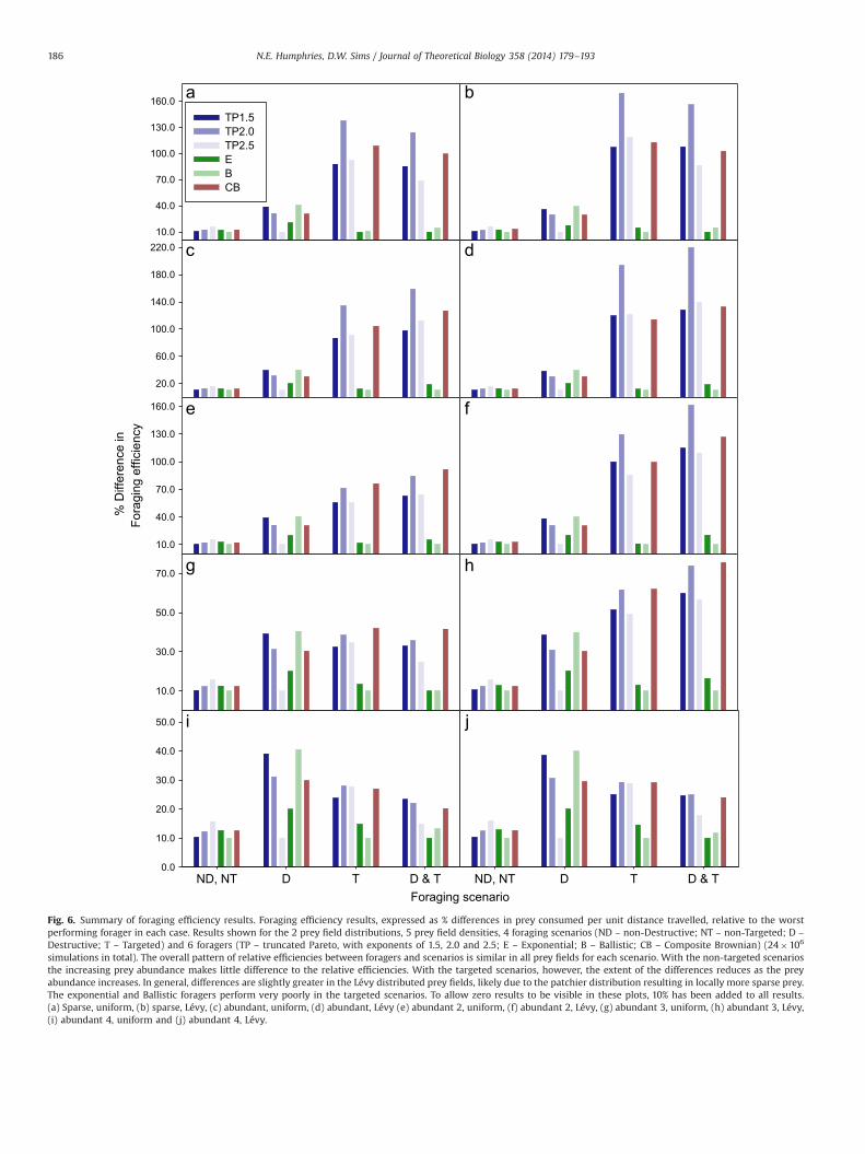
Fig. 6. Summary of foraging efficiency results. Foraging efficiency results, expressed as % differences in prey consumed per unit distance travelled, relative to the worstperforming forager in each case. Results shown for the 2 prey field distributions, 5 prey field densities, 4 foraging scenarios (ND – non-Destructive; NT – non-Targeted; D –

Destructive; T – Targeted) and 6 foragers (TP – truncated Pareto, with exponents of 1.5, 2.0 and 2.5; E – Exponential; B – Ballistic; CB – Composite Brownian) (24�106

simulations in total). The overall pattern of relative efficiencies between foragers and scenarios is similar in all prey fields for each scenario. With the non-targeted scenariosthe increasing prey abundance makes little difference to the relative efficiencies. With the targeted scenarios, however, the extent of the differences reduces as the preyabundance increases. In general, differences are slightly greater in the Lévy distributed prey fields, likely due to the patchier distribution resulting in locally more sparse prey.The exponential and Ballistic foragers perform very poorly in the targeted scenarios. To allow zero results to be visible in these plots, 10% has been added to all results.(a) Sparse, uniform, (b) sparse, Lévy, (c) abundant, uniform, (d) abundant, Lévy (e) abundant 2, uniform, (f) abundant 2, Lévy, (g) abundant 3, uniform, (h) abundant 3, Lévy,(i) abundant 4, uniform and (j) abundant 4, Lévy.

N.E. Humphries, D.W. Sims / Journal of Theoretical Biology 358 (2014) 179–193186

4. Conclusions

It is clear from the simulations performed here that foragingefficiencies do not converge on a single outcome regardless offoraging strategy, as suggested by James et al. (2011), but are infact highly divergent. In the more biologically realistic scenarios,

Table 4Foraging efficiency results for the Abundant 2 and 3 prey fields.

Scenario Destructive Targeted Forager Abundant 2, uniform Abundant 2, Lévy Abundant 3, uniform Abundant 3, Lévy

Efficiency % Diff Efficiency % Diff Efficiency % Diff Efficiency % Diff

1 No No TP1.5 2.17Eþ00 0.33 2.17Eþ00 0.42 8.68Eþ00 0.35 8.68Eþ00 0.50TP2.0 2.21Eþ00 2.26 2.21Eþ00 2.29 8.84Eþ00 2.26 8.85Eþ00 2.38TP2.5 2.29Eþ00 5.73 2.28Eþ00 5.71 9.15Eþ00 5.79 9.13Eþ00 5.65E 2.22Eþ00 2.57 2.22Eþ00 2.62 8.87Eþ00 2.61 8.87Eþ00 2.66B 2.16Eþ00 0.00 2.16Eþ00 0.00 8.65Eþ00 0.00 8.64Eþ00 0.00CB2 2.21Eþ00 2.30 2.21Eþ00 2.44 8.85Eþ00 2.30 8.84Eþ00 2.29

2 Yes No TP1.5 2.13Eþ00 29.15 2.13Eþ00 28.40 8.52Eþ00 29.08 8.53Eþ00 28.57TP2.0 2.00Eþ00 21.35 2.01Eþ00 20.89 8.00Eþ00 21.18 8.02Eþ00 20.84TP2.5 1.65Eþ00 0.00 1.66Eþ00 0.00 6.60Eþ00 0.00 6.64Eþ00 0.00E 1.82Eþ00 10.04 1.83Eþ00 10.19 7.26Eþ00 9.92 7.31Eþ00 10.19B 2.15Eþ00 30.55 2.16Eþ00 30.00 8.62Eþ00 30.55 8.63Eþ00 30.00CB2 1.99Eþ00 20.49 2.00Eþ00 20.38 7.95Eþ00 20.42 7.98Eþ00 20.21

3 No Yes TP1.5 3.12Eþ00 45.58 4.07Eþ00 89.81 1.05Eþ01 22.43 1.21Eþ01 41.41TP2.0 3.46Eþ00 61.42 4.71Eþ00 119.77 1.10Eþ01 28.49 1.30Eþ01 51.61TP2.5 3.13Eþ00 45.98 3.75Eþ00 75.15 1.07Eþ01 24.51 1.19Eþ01 39.14E 2.17Eþ00 1.54 2.17Eþ00 1.04 8.84Eþ00 3.32 8.81Eþ00 2.97B 2.14Eþ00 0.00 2.14Eþ00 0.00 8.56Eþ00 0.00 8.56Eþ00 0.00CB2 3.56Eþ00 66.34 4.05Eþ00 89.12 1.13Eþ01 32.03 1.30Eþ01 51.81

4 Yes Yes TP1.5 1.17Eþ00 52.73 1.31Eþ00 104.59 4.00Eþ00 22.90 4.00Eþ00 49.75TP2.0 1.33Eþ00 74.34 1.61Eþ00 151.31 4.09Eþ00 25.67 4.38Eþ00 63.85TP2.5 1.17Eþ00 53.85 1.28Eþ00 99.66 3.73Eþ00 14.78 3.91Eþ00 46.29E 8.03E�01 5.20 7.06E-01 10.49 3.25Eþ00 0.00 2.84Eþ00 6.43B 7.63E�01 0.00 6.39E-01 0.00 3.25Eþ00 0.12 2.67Eþ00 0.00CB2 1.39Eþ00 81.78 1.38Eþ00 116.53 4.28Eþ00 31.71 4.43Eþ00 65.64

Table 5Foraging efficiency results for the Abundant 4 prey field.

Scenario Destructive Targeted Forager Abundant 4,uniform

Abundant 4, Lévy

Efficiency % Diff Efficiency % Diff

1 No No TP1.5 1.74Eþ01 0.36 1.73Eþ01 0.42TP2.0 1.77Eþ01 2.29 1.77Eþ01 2.45TP2.5 1.83Eþ01 5.73 1.83Eþ01 5.86E 1.77Eþ01 2.65 1.78Eþ01 2.83B 1.73Eþ01 0.00 1.73Eþ01 0.00CB2 1.77Eþ01 2.57 1.77Eþ01 2.66

2 Yes No TP1.5 1.70Eþ01 29.10 1.71Eþ01 28.56TP2.0 1.60Eþ01 21.20 1.60Eþ01 20.65TP2.5 1.32Eþ01 0.00 1.33Eþ01 0.00E 1.45Eþ01 9.98 1.46Eþ01 10.06B 1.72Eþ01 30.52 1.72Eþ01 29.92CB2 1.58Eþ01 19.88 1.59Eþ01 19.52

3 No Yes TP1.5 1.94Eþ01 13.75 1.97Eþ01 15.00TP2.0 2.02Eþ01 18.00 2.05Eþ01 19.30TP2.5 2.01Eþ01 17.76 2.04Eþ01 18.79E 1.79Eþ01 4.80 1.79Eþ01 4.62B 1.71Eþ01 0.00 1.72Eþ01 0.00CB2 2.00Eþ01 17.03 2.04Eþ01 19.17

4 Yes Yes TP1.5 7.09Eþ00 13.32 6.98Eþ00 14.65TP2.0 7.01Eþ00 12.09 7.00Eþ00 14.97TP2.5 6.55Eþ00 4.78 6.55Eþ00 7.68E 6.25Eþ00 0.00 6.08Eþ00 0.00B 6.46Eþ00 3.24 6.19Eþ00 1.80CB2 6.90Eþ00 10.25 6.94Eþ00 14.05

0

20

40

60

80

100

120

140 TP1.5 TP2.0 TP2.5 ExpBallisticCB

Prey field densitySparse Abundant 1 Abundant 2 Abundant 3 Abundant 4

% D

iffer

ence

in e

ffici

ency

0

40

80

120

160

200

Fig. 7. Response of relative efficiency to increasing abundance. The graphs showdifferences in efficiency (prey consumed per unit distance travelled) relative to theworst performer in the destructive, prey-targeting scenario. (a) is a uniform preyfield and (b) a Lévy prey field; TP is a truncated Pareto forager with, for TP1.5 μ¼1.5,for TP2.0 μ¼2.0, for TP2.5 μ¼2.5; Exp is exponential; CB is a bi-exponentialcomposite Brownian. At all prey abundances the TP2.0 forager is significantly moreefficient than all but the CB forager. The exponential and ballistic foragers areconsistently the worst performers and have relative efficiencies that are notaffected by changing prey field abundance. Interestingly, for the Lévy and CBforagers, efficiency is better in the Abundant 1 prey field, before diminishing as theabundance increases further. This could be due to the sparse prey field being toosparse to generate properly sampled results. Even at the highest abundance it isclear that a Lévy or CB forager will easily outperform an exponential or ballisticforager.

N.E. Humphries, D.W. Sims / Journal of Theoretical Biology 358 (2014) 179–193 187

that include prey-targeting, and in the less abundant prey fields,which require a search strategy, the TP2.0 forager is most efficient,while in other scenarios and in some extremely abundant preyfields, other foraging strategies can perform slightly better. Animportant finding of the current study is that the TP2.0 searchstrategy shows persistent stability in its optimal performanceacross a much broader set of environmental conditions thanpreviously identified compared to many other types of searchstrategies. Thus, it appears the TP2.0 Lévy walk strategy deter-mined by Viswanathan et al. (1999) to be optimal when prey aresparse but can be targeted, is in fact not a limiting case. We showthat the TP2.0 Lévy strategy is optimal for foraging in natural-likeenvironments varying greatly in resource density, distribution andpatch revisitability. As such it is arguably a general ‘rule of thumb’for efficient searching in heterogeneous natural environments

when an organism can target prey when encountered within itssensory detection range, but has no or only an incomplete knowl-edge of where resources are located beyond their sensory range.

4.1. Scenario 1, the null model

The relative efficiencies of the foragers under this scenario wereremarkably consistent. In all cases the TP2.5 forager was the mostsuccessful by as much as 6.2%, with either the TP1.5 or ballistic theleast; in fact success here is closely and inversely related to the meanstep-length. It might be that the lower patch-leaving behaviourinherent in the TP2.5 forager ensures that when a patch is encoun-tered it is exploited more completely than with the other foragers;however it is still somewhat surprising that this is sufficient to balance

Log 1

0 Fa

min

e du

ratio

ns1e+2

1e+3

1e+4

ForagerTP1.5 TP2.0 TP2.5 E B CB2

1e+2

1e+3

1e+4

1e+2

1e+3

1e+4

1e+5

TP1.5 TP2.0 TP2.5 E B CB2

Log10 Fam

ine durations

1e+2

1e+3

1e+4

1e+5

Fig. 8. Median famine durations. Median famine durations calculated from the number of interpolated steps between prey encounters (i.e. distance travelled or timeelapsed); a & b non-destructive targeted, scenario (S3) ;c & d destructive, targeted scenario (S4). Uniform and Lévy distributed, Abundant 1 prey fields were used. Note thelog scale for famine durations. Horizontal bar shows median, boxes show 25th and 75th percentiles, whiskers show 10th and 90th percentiles, outliers show 5th and 95thpercentiles. In all cases the TP2.0 forager experiences the shortest famine periods and, consequently, the most homogenous prey availability. Note that in a & c theexponential 95th percentile is off the scale.

Grid

siz

e(n

o of

ele

men

ts)

2000

2500

3000

3500

4000

4500

5000

Area

1e+7

2e+7

3e+7

4e+7

5e+7

6e+7

TP 1.5 TP 2.0 TP 2.5 Exp CB

Oversam

pling

200

400

600

800

TP 1.5 TP 2.0 TP 2.5 Exp CB

Cel

l occ

upan

cy %

10

15

20

25

30

35

40

Fig. 9. Path structure analysis results. a. Confirmation that the grid used for each forager was appropriately scaled and comprised a similar number of grid cells to allow pathstructure, rather than scale, to dominate the analysis. b. The bounding area is, as expected, higher with super-diffusive foragers such as TP1.5 and is lowest for theexponential. c. Although the area bounded by the exponential path is low (b) the percentage of the area explored is greatest. This result illustrates the diffusive nature ofexponential paths. The TP1.5 path, which is the most super-diffusive, explores the lowest percentage of the area bounded by the extent of the path, as expected from themore ballistic characteristics. d. The oversampling value of the Lévy foragers increases with increasing exponents, as a consequence of fewer long steps. Oversampling in theexponential path is low compared to the ‘Brownian like’ TP2.5 path, further illustrating the essential structural difference between an exponential and a Lévy path and thediffusive character of an exponential path.

N.E. Humphries, D.W. Sims / Journal of Theoretical Biology 358 (2014) 179–193188

the much lower likelihood of patch location of the other foragers. It isalso noteworthy that the TP2.5 forager performs so much better thanthe exponential forager, given that Lévy movements with higherexponents tend towards a more Brownian-like pattern.

4.2. The stability of destructive or targeted foraging

One of the most striking results from these investigations is therobust stability of the destructive and targeted foraging scenarios,

Fig. 10. Example plots from the path structure analysis. The plots show the results of the path structure analysis for foragers (a) TP1.5; (b) TP2.0; (c) TP2.5; (d) Exponentialand (e) CB. Warmer colours indicate higher oversampling values. The faint grey lines indicate the analysis grid and confirm that the relative grid size is the same in all cases.The structure of the TP foragers can be seen to alter as the exponent is increased, resulting in fewer long steps and increased oversampling. The structure of the exponentialpath is quite different from the Lévy foragers, having no long relocations and a more extensive use of the space. The CB forager falls part way between the TP and exponentialforagers, having more long steps than the exponential, but less intensive space use. (For interpretation of the references to color in this figure legend, the reader is referred tothe web version of this article.)

Fig. 11. Example foraging paths for TP2.5 and exponential foragers. Four sample paths from each of a TP2.5 (left), and exponential forager (right), arranged so as not tooverlap. It is clear, simply from the overall darkness of each image, that the TP2.5 forager searches a smaller proportion of the prey field.

N.E. Humphries, D.W. Sims / Journal of Theoretical Biology 358 (2014) 179–193 189

all of which settle to the final outcome after fewer simulation runs,and with shorter path lengths, than scenario 1. In the destructivenon-targeted scenario the ballistic, and most ballistic-like Lévyforager, the TP1.5, were always the most efficient, as predicted bythe more rapid patch-leaving behaviour that these foragers willexhibit. The advantage was highly significant and consistent ataround 30% better than the worst performer (TP2.5). Destructiveforaging is biologically realistic since fish shoals and planktonpatches may become functionally depleted eventually (i.e. aforager is unable to feed at net energetic benefit since anyremaining individuals would not yield sufficient energy to coverthe costs of its collection; Sims, 1999). This result thereforeconfirms one of the Lévy-flight foraging hypothesis' predictions:that with destructive foraging Lévy foragers with low exponentsare most efficient (Bartumeus et al., 2005). It is interesting to notethat in this scenario the TP2.5 forager was always the leastefficient. Comparing a typical TP2.5 path (which is moreBrownian-like than the other Lévy foragers) with an exponentialpath reveals the TP2.5 to have significantly more long relocations,but, nonetheless, to cover considerably less of the prey field thanthe exponential forager (as shown in Fig. 11). Using ImageJ(Rasband, 1997–2012) to compute a histogram from each imagegives a value that represents the proportion of the image covered(i.e. the proportion of black pixels, see Fig. 11). The results showthat the TP2.5 forager covers 2.0%, while the exponential foragercovers 6.0%, confirming that the TP2.5 forager would encounterless biomass and have a lower foraging efficiency.

It is interesting that incorporating destructive foraging reducesstochastic variability sufficiently for the performance of theforagers to settle reasonably quickly (i.e. within 3.5�104 simula-tions). As some studies have performed only 104 simulations itseems likely that previously reported results (e.g. James et al.,2011) show foragers that have not reached efficiency stability. As afinal comment on the destructive non-targeted scenario it isinteresting that in all simulations the TP2.0 forager outperformsthe exponential forager by between 9.21% and 11.24%, a figure thatis in close agreement with the result found by Sims et al. (2008),confirming that the simulations performed in that study wereperhaps closer to a destructive foraging scenario because patchescould not be revisited.

4.3. The importance of prey-targeting

In the original studies by Viswanathan (Viswanathan et al.,1999, 2000) the foraging model included prey-targeting. Theresults presented here make it very clear, firstly, that with prey-targeting the TP2.0 forager consistently emerges as the mostefficient searcher and, secondly, that the relative performance ofthe other foragers is also strongly conserved. Overall the foragingefficiencies shown by the TP2.0 forager and the relative perfor-mances of the other foragers were robust to prey field abundance,prey field distribution, and prey patch revisitability, indicating aLévy walk with m¼2 is optimal over a much wider range ofenvironment types than previously demonstrated. It is worthreiterating that the destructive scenario used here differs fromthat of Viswanathan et al. (1999) where solitary prey items wereused. In our study, much of a prey patch remained when a singleitem (grid cell) was destructively consumed, which is perhapsmore comparable to natural prey patches. As mentioned in theresults it is somewhat surprising that prey-targeting shouldproduce such a stable outcome, given that the advantage gainedwhen a patch is encountered is the same for all foragers (Fig. 5).

Prey-targeting adds a further dimension to the simulation in thatit represents a feedback response from the prey to the forager in theform of a behavioural switch; on encountering prey the move step isterminated and a new step is started. With a power-law distribution

of move-steps subsequent steps are likely to be small, representing aslowing of movement, or increased tortuosity. The virtual foragers inthis study cannot alter their move-step distribution in order torespond to prey-fields with changing densities, a behaviour thatwould be expected in real foragers, with switching to area-restrictedsearch being commonly observed when prey-field densities aregreater (Hamer et al., 2009; Pinaud and Weimerskirch, 2005; Simsand Quayle, 1998). It is all the more interesting, therefore, that prey-targeting is so important in differentiating between the differentforagers tested here.

4.4. Prey abundance is less important than first thought

In the non-targeted scenarios prey abundance made littledifference to the relative foraging efficiencies. In the targetedscenarios, however, as prey field abundance was increased thedifference between the foragers reduced as predicted. Howeverthe level of abundance required for parity was much higher thanexpected based on previous studies that concluded Lévy foragingis only more efficient when prey is sparse (Bartumeus et al., 2002;Viswanathan et al., 1999, 2000, 2002). With increasing preyabundance searching becomes less important than patch exploita-tion. The success of the composite Brownian forager in theAbundant 2 and 3 prey fields most likely, therefore, results frommore efficient patch exploitation than the TP2.0 forager, while thesuccess of the TP2.0 forager in the sparser prey fields results frommore efficient location of distant patches. It is interesting that theslight advantage gained by the CB forager is lost when the preyfield abundance is increased further. This suggests that the CBforager is less resilient to changes in prey field density than theTP2.0 forager. If an organism was to adopt a single strategy, thenthe TP2.0 would be the most successful over a broader range ofenvironments. In the mathematical analysis by Viswanathan et al.(2000) the conclusion regarding prey abundance – i.e. thatBrownian movement is sufficiently efficient – is applicable whenthe abundance is such that the distance to the next prey item isless than or equal to the radius of detection (described in the paperas λrrv). The radius of detection used in this simulation is set to1 unit, the most conservative value, and clearly it is not possible tohave prey abundance set to such a density without all cells beingpopulated. It is worth noting that even the level of prey abundancein these simulations represents a very dense concentration. Forexample, if the scale of the simulation here represented a 1 cmgrid and the biomass represented zooplankton, such as copepods(e.g. Calanus helgolandicus), with each unit of biomass comprisinga single copepod, then the prey density in the most abundant preyfield, which had an average density of 19.2 units per cell, would beequivalent to 19,200,000 copepods m�3. Even at this density inthe simulation parity between the model foragers was not quiteachieved. So how do resource fields in the natural environmentcompare with the simulated density? One field measurement ofzooplankton density recorded by Sims (1999; based on totalzooplankters) was found to be around 2600 m�3. This densitywas the highest reported in that study and agrees well with otherstudies that put maximum regional concentrations at around 103

individuals m�3 (Pendleton et al., 2009), yet is much lower thanthe density at which a significant difference between the foragerswas still found here. While much higher plankton densities havebeen recorded on scales ofo1 m, associated with the sea surfaceboundary (Gallager et al., 1996) these represent micro-scaleaggregations and are not representative of the patch as a whole.At a larger scale such densities could represent fish within a shoalas opposed to the distribution of shoals within the ocean. Theimportant point here is that at the very high levels of prey fielddensity in our simulation, random searches are no longer requiredand the most efficient movement patterns will be those associated

N.E. Humphries, D.W. Sims / Journal of Theoretical Biology 358 (2014) 179–193190

with patch exploitation, rather than patch location. Thus, large,oceanic predators, such as blue sharks (Prionace glauca) are likelyto experience sparse prey fields and will benefit from optimal Lévysearch strategies, whilst terrestrial herbivores, grazing in abundantprey patches, benefit most from patch exploitation strategies, suchas composite Brownian walks (sometimes termed multi-modalwalks in the ecology literature).

4.5. Feast and famine

Heterogeneity in prey availability requires energetically expen-sive adaptations to deal with the resulting periods of feast orfamine, such as excess digestive capacity (Armstrong andSchindler, 2011) and lipid storage (Arrington et al., 2006). Pisci-vores in particular have been found to have empty stomachs moreoften than other feeding guilds (Arrington et al., 2002) and, whiledifficult to observe in the wild (although stomach loggers arebecoming available for sharks: Papastamatiou et al., 2007), a feastand famine feeding pattern has been observed in captive seven-gill sharks (Notorynchus cepedianus) (Vandykhuizen and Mollet,1992). In this context a TP2.0 foraging strategy delivers a doublebenefit; increasing the number of new prey-patch encounters notonly increases the quantity of prey available but minimises thetime to the next feeding event. Thus, Lévy foraging results in morepredictable resources in unpredictable environments. Importantly,the results show that both the TP1.5 and TP2.0 foragers bothexperience significantly fewer long famine periods than the otherforagers, in all cases, but especially in the Lévy distributed preyfields. In the Lévy prey fields, which are considered more biolo-gically realistic, the TP2.5, Exponential and CB foragers experiencesignificantly more long famine periods, placing them at muchgreater risk of starvation (Faustino et al., 2007). The high perfor-mance of the TP1.5 forager is particularly interesting and suggeststhat while the TP2.0 is theoretically most efficient, natural selec-tion pressures might result in lower observed exponents. Theore-tically, Lévy foragers, with a range of exponents, are therefore lesslikely to starve than exponential or CB foragers, which clearlyconfers many physiological benefits. These findings make itincreasingly likely that movement patterns approximating a Lévywalk would have been naturally selected since the advantages tonet energy gain appear very marked.

4.6. Path structure

The aim of the path structure analysis was to gain a moredetailed understanding of how different movement patterns, inthe form of different move step-length distributions, may lead to

differing foraging efficiencies. Several questions arise from thecurrent study that might be addressed with this analysis: forexample, why does the TP2.5 forager perform so consistently wellin scenario 1, why does the TP2.0 forager outperform by such asignificant margin the other foragers in most of the prey-targetingscenarios, and what leads the CB forager to perform better in thevery abundant prey fields, yet lose this advantage in the mostabundant prey fields?

With reference to the first question, our study identifies asignificant difference between the TP2.5 and exponential foragers.Both foragers search similar areas; however, the oversamplingvalue of the TP2.5 forager greatly exceeds that of the exponentialforager. This difference is indicative of a fundamental difference inthe underlying movement pattern, whereby the TP2.5 foragerperforms many more very small move steps, thus keeping itwithin a small area, until a rare, much longer step is performedwhich takes it well beyond the previous position. This patternallows the forager to explore a larger overall area, while at thesame time focussing most movements on very small areas. Bycontrast, the exponential forager diffuses more gradually, coveringthe area more evenly. For the TP2.5 forager in a non-destructivescenario, an encountered patch is more likely thoroughly exploitedby the concentrated tortuous movements, while the rare longerrelocations find new patches. The exponential forager, however,locates fewer patches and exploits those that are encountered lessthoroughly. The TP2.5 characteristic of thoroughly exploiting anarea before moving to the next might be what provides theadvantage when prey is consumed non-destructively.

The CB path in Fig. 10e shows how this forager combinescharacteristics of both the Lévy and exponential foragers. Theoverall structure is similar to that of the exponential, but there aremore long steps, therefore the CB is more efficient than theexponential at locating new patches, but at the same time it hasintensive patch exploitation characteristics. This explains why theCB forager performs well when prey is very abundant, as it isexploitation, rather than searching that becomes advantageous.However, it is not clear why this advantage should be lost whenthe prey field abundance is increased further.

Insight into why the TP2.0 forager is the most efficient in themajority of prey fields in the targeted scenarios is not aided by thepath structure analysis. All the Lévy foragers perform substantiallybetter than the exponential forager under all the targeted scenarios.All combine larger search areas (resulting from long relocations) withstrongly focused patch exploitation, as a result of the large number ofvery small steps. All that can be confirmed is that, in the majorityof cases, the TP2.0 strikes an optimal balance of patch location(exploration) and patch exploitation, with the long relocations being

Table 6Feast and famine results, The table shows the analysis of famine period durations, computed as the number of simulation steps between encounters with prey. Prey fieldswere the Abundant 1 density, to ensure sufficient encounters.

Scenario Destructive Targeted Forager Uniform Lévy

Median 25% 75% Median 25% 75%

3 No Yes TP1.5 247.68 169.23 387.02 235.16 140.19 463.54TP2.0 200.47 133.33 330.21 198.82 101.24 558.20TP2.5 285.27 157.70 690.78 902.84 145.77 47573.00E 524.03 268.72 1443.24 23025.00 334.70 46212.00B 443.84 287.64 728.58 488.51 288.04 929.41CB2 234.90 151.74 407.56 363.88 136.30 3558.90

4 Yes Yes TP1.5 441.08 316.75 646.44 428.25 263.74 788.75TP2.0 359.49 250.06 561.30 361.42 190.35 941.85TP2.5 512.67 302.73 1131.98 1440.67 276.32 47572.00E 891.63 490.82 2103.86 23071.00 592.59 46213.00B 786.18 543.88 1156.49 862.80 541.26 1464.72CB2 414.64 280.62 678.17 652.22 255.65 4642.38

N.E. Humphries, D.W. Sims / Journal of Theoretical Biology 358 (2014) 179–193 191

rare enough to allow patches to be exploited, but long enough toallow a large area to be explored and new patches to be encountered.The path structure analysis does, however, indicate clearly the fractalself-similarity of the Lévy foraging paths; the scale invariant nature ofthe resulting searches is clearly advantageous.

4.7. Summary

Even the most biologically realistic scenario presented herefalls far short of the behavioural complexity exhibited by an apexpredator such as a shark. No account is taken of refined sensoryinput, memory effects or the sophisticated hunting and foragingbehaviour that is ubiquitous among higher organisms. The for-agers presented here are therefore very much a null model offoraging; all that is being studied is how simple, basal movementpatterns affect the efficiency of an uninformed random search. It islikely that even nematodes, such as Caenorhabditis elegans, bysensing chemical gradients (Ohkubo et al., 2010), have at leastsome knowledge of their wider resource environment. Never-theless, it is clear that differences in these simple patterns producesignificant differences not only in foraging efficiency but also inexperienced prey field homogeneity, which are robust to differ-ences in prey abundance or distribution. The differences are notsmall; in the Abundant 1, Lévy-distributed prey field the TP2.0forager has a foraging efficiency43 times that of the exponentialforager. Given that all that is required for an organism to produce aLévy movement pattern is a time-fractal activity pattern(Bartumeus and Levin, 2008), which has been observed in evensimple animals such as Drosophila (Cole, 1995), it seems unlikelythat such behaviour would not have been selected for duringevolution since adopting Lévy movements optimises foraging in awide range of environments. In further support of the propositionthat Lévy movement could represent an intrinsic, basal movementpattern, a study by de Jager et al. (2014) has found evidence forLévy movements in young mussels (Mytilus edulis) during settle-ment. When the crawling movements were uninterrupted by thepresence of conspecifics the resulting movement pattern was Lévylike; however, when moves were more frequently truncated, anexponential pattern emerged.

When studying complex organisms, such as marine verte-brates, these simple movement patterns are only going to beobserved on those occasions when the animal is actively engagedin foraging, when information of the location of prey is absent andwhen other behaviours, such as prey avoidance, migration orresponse to environmental cues are not dominating the animal'smovement. It is therefore to be expected that empirical evidencefor these patterns will be relatively rare. There is at the presenttime burgeoning empirical support for Lévy movement patterns ina range of taxa, including insects (Reynolds and Frye, 2007;Reynolds et al., 2007), dinoflagellates (Bartumeus et al., 2003),marine molluscs (de Jager et al., 2011, 2014; Seuront et al., 2007),marine turtles, fish and seabirds (Humphries et al., 2013; Simset al., 2008) and primates (Ramos-Fernandez et al., 2004) includinghumans (Brown et al., 2007; Gonzalez et al., 2008; Raichlen et al.,2014; Rhee et al., 2008). Perhaps it is expected that Lévy patternswould not be common in terrestrial animals as stable environ-mental structures (i.e. landscape features, forest trees, etc.) providevery persistent clues as to the location of prey or other resources.Nor are they likely to be common among higher vertebrates suchas bears, (Ursus arctos), where the animals rely on good spatio-temporal mental maps of resource availability and rarely performlarge-scale random searches (Bojarska and Selva, 2012). Therefore,it seems likely that Lévy search patterns should be most common indynamic environments such as the open sea because resources areoften highly sparse and have complex distributions that are tran-sported by tides and currents over widely different spatio-temporal

scales. Submerged predators are, therefore, only likely to have anincomplete knowledge of resource location and the detection ofsuch resources at distance (e.g. vision, olfaction) will be limited bythe seawater medium compared to terrestrial or aerial environ-ments. Hence, it is unsurprising that, to date, the most robust testsof the Lévy flight foraging hypothesis have come from the study ofpelagic open ocean predators. Future empirical studies on a widerrange of organisms will provide a more complete picture of thespecies that exhibit Lévy movement patterns and when and wherethey are employed. However, as we demonstrate here, the clear andpersistent foraging advantages that Lévy walk search patternsconfer on model organisms in a very wide range of model environ-ments provides further strong support for the contention thatsearching movements approximated by Lévy walks should havenaturally evolved.

Acknowledgements

Funding was provided by the UK Natural EnvironmentResearch Council's Oceans 2025 Strategic Research Programme(Theme 6 Science for Sustainable Marine Resources) in whichD.W.S. was a principal investigator. D.W.S was also supported by aMarine Biological Association (MBA) Senior Research Fellowship.We thank two anonymous reviewers for helpful comments andsuggestions that improved the paper.

References

Amanatides, J., Woo, A., 1987. A fast voxel traversal algorithm for ray tracing. In:Proceedings of the Eurographics '87. Amsterdam, pp. 1–10.

Armstrong, J.B., Schindler, D.E., 2011. Excess digestive capacity in predators reflectsa life of feast and famine. Nature 476, 84–87.

Arrington, D.A., Winemiller, K.O., Loftus, W.F., Akin, S., 2002. How often do fishesrun on empty? Ecology 83, 2145–2151.

Arrington, D.A., Davidson, B.K., Winemiller, K.O., Layman, C.A., 2006. Influence oflife history and seasonal hydrology on lipid storage in three neotropical fishspecies. J. Fish Biol. 68, 1347–1361.

Bartumeus, F., Levin, S.A., 2008. Fractal reorientation clocks: linking animalbehavior to statistical patterns of search. Proc. Natl. Acad. Sci. USA 105,19072–19077.

Bartumeus, F., Da Luz, M.G.E., Viswanathan, G.M., Catalan, J., 2005. Animal searchstrategies: a quantitative. random-walk analysis. Ecology 86, 3078–3087.

Bartumeus, F., Catalan, J., Fulco, U.L., Lyra, M.L., Viswanathan, G.M., 2002. Optimiz-ing the encounter rate in biological interactions: Lévy versus Brownianstrategies. Phys. Rev. Lett. 88, 4.

Bartumeus, F., Peters, F., Pueyo, S., Marrase, C., Catalan, J., 2003. Helical Levy walks:adjusting searching statistics to resource availability in microzooplankton. Proc.Natl. Acad. Sci. USA 100, 12771–12775.

Bazazi, S., Bartumeus, F., Hale, J.J., Couzin, I.D., 2012. Intermittent motion in desertlocusts: behavioural complexity in simple environments. Plos Comput. Biol. 8, 10.

Benhamou, S., 2007. How many animals really do the Lévy walk? Ecology 88,1962–1969.

Bojarska, K., Selva, N., 2012. Spatial patterns in brown bear Ursus arctos diet: therole of geographical and environmental factors. Mammal Rev. 42, 120–143.

Brown, C., Liebovitch, L., Glendon, R., 2007. Lévy Flights in Dobe Ju/‘hoansi foragingpatterns. Hum. Ecol.: Interdiscip. J. 35, 129–138.

Buchanan, M., 2008. Ecological modelling: the mathematical mirror to animalnature. Nature 453, 714–716.

Cole, B.J., 1995. Fractal time in animal behavior – the movement activity ofDrosophila. Anim. Behav. 50, 1317–1324.

de Jager, M., Weissing, F.J., Herman, P.M.J., Nolet, B.A., van de Koppel, J., 2011. Lévywalks evolve through interaction between movement and environmentalcomplexity. Science 332, 1551–1553.

de Jager, M., Weissing, F.J., Herman, P.M.J., Nolet, B.A., van de Koppel, J., 2012.Response to comment on Lévy walks evolve through interaction betweenmovement and environmental complexity. Science 335, 918.

de Jager, M., Bartumeus, F., Kol̈zsch, A., Weissing, F.J., Hengeveld, G.M., Nolet, B.A.,Herman, P.M.J., van de Koppel, J., 2014. How superdiffusion gets arrested:ecological encounters explain shift from Lévy to Brownian movement. Proc. R.Soc. B: Biol. Sci 281 (1774).

Faustino, C.L., daSilva, L.R., daLuz, M.G.E., Raposo, E.P., Viswanathan, G.M., 2007.Search dynamics at the edge of extinction: Anomalous diffusion as a criticalsurvival state. Epl 77 (3), 6.

Gallager, S.M., Davis, C.S., Epstein, A.W., Solow, A., Beardsley, R.C., 1996. High-resolution observations of plankton spatial distributions correlated with

N.E. Humphries, D.W. Sims / Journal of Theoretical Biology 358 (2014) 179–193192

hydrography in the Great South Channel, Georges Bank. Deep Sea Res. Part II:Top. Stud. Oceanogr. 43, 1627–1663.

Gonzalez, M.C., Hidalgo, C.A., Barabasi, A.L., 2008. Understanding individual humanmobility patterns. Nature 453, 779–782.

Hamer, K.C., Humphreys, E.M., Magalhaes, M.C., Garthe, S., Hennicke, J., Peters, G.,Gremillet, D., Skov, H., Wanless, S., 2009. Fine-scale foraging behaviour of amedium-ranging marine predator. J. Anim. Ecol. 78, 880–889.

Hartig, F., Calabrese, J.M., Reineking, B., Wiegand, T., Huth, A., 2011. Statisticalinference for stochastic simulation models – theory and application. Ecol. Lett.14, 816–827.

Hays, G.C., Bastian, T., Doyle, T.K., Fossette, S., Gleiss, A.C., Gravenor, M.B., Hobson, V.J.,Humphries, N.E., Lilley, M.K.S., Pade, N.G., Sims, D.W., 2012. High activity and Lévysearches: jellyfish can search the water column like fish. Proc. R. Soc. B: Biol. Sci.279, 465–473.

Humphries, N.E., Weimerskirch, H., Sims, D.W., 2013. A new approach for objectiveidentification of turns and steps in organism movement data relevant torandom walk modelling. Methods Ecol. Evol. 4, 930–938.

Humphries, N.E., Weimerskirch, H., Queiroz, N., Southall, E.J., Sims, D.W., 2012.Foraging success of biological Lévy flights recorded in situ. Proc. Natl. Acad. Sci.USA 109, 7169–7174.

Humphries, N.E., Queiroz, N., Dyer, J.R.M., Pade, N.G., Musyl, M.K., Schaefer, K.M.,Fuller, D.W., Brunnschweiler, J.M., Doyle, T.K., Houghton, J.D.R., Hays, G.C., Jones,C.S., Noble, L.R., Wearmouth, V.J., Southall, E.J., Sims, D.W., 2010. Environmentalcontext explains Lévy and Brownian movement patterns of marine predators.Nature 465, 1066–1069.

James, A., Plank, M.J., Edwards, A.M., 2011. Assessing Levy walks as models ofanimal foraging. J. R. Soc. Interface 8, 1233–1247.

Jansen, V.A.A., Mashanova, A., Petrovskii, S., 2012. Comment on Lévy Walks EvolveThrough Interaction Between Movement and Environmental Complexity.Science 335, 918.

Klafter, J., Zumofen, G., Shlesinger, M.F., 1993. Levy walks in dynamical-systems.Physica A 200, 222–230.

Kohler, N.E., Turner, P.A., 2001. Shark tagging: a review of conventional methodsand studies. Environ. Biol. Fishes 60, 191–223.

López-López, P., Benavent-Corai, J., García-Ripollés, C., Urios, V., 2013. Scavengers onthe move: behavioural changes in foraging search patterns during the annualcycle. PLoS One 8, e54352.

Maye, A., Hsieh, C.H., Sugihara, G., Brembs, B., 2007. Order in spontaneous behavior.PLoS One 2, 14.

Miramontes, O., Boyer, D., Bartumeus, F., 2012. The effects of spatially hetero-geneous prey distributions on detection patterns in foraging seabirds. PLoS One7, 9.

Ohkubo, J., Yoshida, K., Iino, Y., Masuda, N., 2010. Long-tail behavior in locomotionof Caenorhabditis elegans. J. Theor. Biol. 267, 213–222.

Oshanin, G., Lindenberg, K., Wio, H.S., Burlatsky, S., 2009. Efficient search byoptimized intermittent random walks. J. Phys. A-Math. Theor., 42.

Papastamatiou, Y.P., Meyer, C.G., Holland, K.N., 2007. A new acoustic pH transmitterfor studying the feeding habits of free-ranging sharks. Aquat. Living Resourc.20, 287–290.

Pendleton, D.E., Pershing, A.J., Brown, M.W., Mayo, C.A., Kenney, R.D., Record, N.R.,Cole, T.V.N., 2009. Regional-scale mean copepod concentration indicatesrelative abundance of North Atlantic right whales. Mar. Ecol.-Prog. Ser. 378,211–225.

Pinaud, D., Weimerskirch, H., 2005. Scale-dependent habitat use in a long-rangingcentral place predator. J. Anim. Ecol. 74, 852–863.

Plank, M.J., James, A., 2008. Optimal foraging: Levy pattern or process? J. R. Soc.Interface 5, 1077–1086.

Plank, M.J., Codling, E.A., 2009. Sampling rate and misidentification of Levy andnon-Levy movement paths. Ecology 90, 3546–3553.

Priede, I.G., 1984. A basking shark (Cetorhinus maximus) tracked by satellitetogether with simultaneous remote sensing. Fish. Res. 2, 201–216.

Raichlen, D.A., Wood, B.M., Gordon, A.D., Mabulla, A.Z.P., Marlowe, F.W., Pontzer, H.,2014. Evidence of Lévy walk foraging patterns in human hunter–gatherers.Proc. Natl. Acad. Sci. 111, 728–733.

Ramos-Fernandez, G., Mateos, J.L., Miramontes, O., Cocho, G., Larralde, H., Ayala-Orozco, B., 2004. Lévy walk patterns in the foraging movements of spidermonkeys (Ateles geoffroyi). Behav. Ecol. Sociobiol. 55, 223–230.

Raposo, E.P., Buldyrev, S.V., da Luz, M.G.E., Santos, M.C., Stanley, H.E., Viswanathan,G.M., 2003. Dynamical robustness of Lévy search strategies. Phys. Rev. Lett. 91(24).

Rasband, W.S., 1997-2012. ImageJ, U.S. National Institutes of Health. Bethesda,Maryland, USA.

Reynolds, A.M., 2009. Adaptive Levy walks can outperform composite Brownianwalks in non-destructive random searching scenarios. Phys. A-Stat. Mech. Appl.388, 561–564.

Reynolds, A.M., 2012. Distinguishing between Levy walks and strong alternativemodels. Ecology 93, 1228–1233.

Reynolds, A.M., 2013. Selection pressures give composite correlated random walksLévy walk characteristics. J. Theor. Biol. 332, 117–122.

Reynolds, A.M., Frye, M.A., 2007. Free-flight odor tracking in Drosophila isconsistent with an optimal intermittent scale-free search. PLoS One 2, e354.

Reynolds, A.M., Rhodes, C.J., 2009. The Levy flight paradigm: random searchpatterns and mechanisms. Ecology 90, 877–887.

Reynolds, A.M., Bartumeus, F., 2009. Optimising the success of random destructivesearches: Lévy walks can outperform ballistic motions. J. Theor. Biol. 260,98–103.

Reynolds, A.M., Swain, J.L., Smith, A.D., Martin, A.P., Osborne, J.L., 2009. Honeybeesuse a Levy flight search strategy and odour-mediated anemotaxis to relocatefood sources. Behav. Ecol. Sociobiol. 64, 115–123.

Reynolds, A.M., Smith, A.D., Menzel, R., Greggers, U., Reynolds, D.R., Riley, J.R., 2007.Displaced honey bees perform optimal scale-free search flights. Ecology 88,1955–1961.

Rhee, L., Shin, M., Hong, S., Lee, K., Chong, S., Ieee, On the Levy-walk nature ofhuman mobility, In: Proceedings of the 27th IEEE Conference on ComputerCommunications (INFOCOM 2008), Ieee, Phoenix, AZ 2008, pp. 1597–1605.

Seuront, L., Duponchel, A.C., Chapperon, C., 2007. Heavy-tailed distributions in theintermittent motion behaviour of the intertidal gastropod Littorina littorea.Phys. A – Stat. Mech. Appl. 385, 573–582.

Sims, D.W., 1999. Threshold foraging behaviour of basking sharks on zooplankton:life on an energetic knife-edge? Proc. R. Soc. Lond. Ser. B-Biol. Sci. 266,1437–1443.

Sims, D.W., Merrett, D.A., 1997. Determination of zooplankton characteristics in thepresence of surface feeding basking sharks Cetorhinus maximus. Mar. Ecol.-Prog.Ser. 158, 297–302.

Sims, D.W., Quayle, V.A., 1998. Selective foraging behaviour of basking sharks onzooplankton in a small-scale front. Nature 393, 460–464.

Sims, D.W., Humphries, N.E., Bradford, R.W., Bruce, B.D., 2012. Levy flight andBrownian search patterns of a free-ranging predator reflect different prey fieldcharacteristics. J. Anim. Ecol. 81, 432–442.

Sims, D.W., Southall, E.J., Humphries, N.E., Hays, G.C., Bradshaw, C.J.A., Pitchford, J.W.,James, A., Ahmed, M.Z., Brierley, A.S., Hindell, M.A., Morritt, D., Musyl, M.K.,Righton, D., Shepard, E.L.C., Wearmouth, V.J., Wilson, R.P., Witt, M.J., Metcalfe, J.D.,2008. Scaling laws of marine predator search behaviour. Nature 451, 1098–1102.

Vandykhuizen, G., Mollet, H.F., 1992. Growth, age estimation and feeding of captivesevengill sharks, Notorynchus cepedianus, at the Monterey Bay aquarium. Austr.J. Mar. Freshw. Res. 43, 297–318.

Viswanathan, G.M., Raposo, E.P., da Luz, M.G.E., 2008. Lévy flights and super-diffusion in the context of biological encounters and random searches. Phys.Life Rev. 5, 133–150.

Viswanathan, G.M., da Luz, M.G.E., Raposo, E.P., Stanley, H.E., 2011. The Physics ofForaging. Cambridge University Press, New York.

Viswanathan, G.M., Buldyrev, S.V., Havlin, S., da Luz, M.G.E., Raposo, E.P., Stanley, H.E.,1999. Optimizing the success of random searches. Nature 401, 911–914.

Viswanathan, G.M., Afanasyev, V., Buldyrev, S.V., Havlin, S., da Luz, M.G.E., Raposo,E.P., Stanley, H.E., 2000. Lévy flights in random searches. Physica A 282, 1–12.

Viswanathan, G.M., Afanasyev, V., Buldyrev, S.V., Havlin, S., da Luz, M.G.E., Raposo, E.P.,Stanley, H.E., 2001. Lévy flights search patterns of biological organisms. Phys. A:Stat. Mech. Appl. 295, 85–88.

Viswanathan, G.M., Bartumeus, F., Buldyrev, S.V., Catalan, J., Fulco, U.L., Havlin, S., daLuz, M.G.E., Lyra, M.L., Raposo, E.P., Stanley, H.E., 2002. Lévy flight randomsearches in biological phenomena. Phys. A: Stat. Mech. Appl. 314, 208–213.

Wearmouth, V.J., McHugh, M.J., Humphries, N.E., Naegelen, A., Ahmed, M.Z.,Southall, E.J., Reynolds, A.M., Sims, D.W., 2014. Scaling laws of ambush predator‘waiting’ behaviour are tuned to a common ecology. Proc. R. Soc. B: Biol. Sci. 281(1782).

N.E. Humphries, D.W. Sims / Journal of Theoretical Biology 358 (2014) 179–193 193