JOURNAL OF SUBSEA AND OFFSHORE

J O U R NA L O F S U B S EA

A N D O F F S H O R E

S C I E N C E A N D E N G I N E E R I N G

V O L U M E . 6

J U N E 3 0 , 2 0 1 6

I S S N : 2 4 4 2 - 6 4 1 5

P U B L I S H E D B Y I S O M A s e

Journal of Subsea and Offshore -Science and Engineering-

Vol.6: June 30, 2016

ISOMAse

International Society of Ocean, Mechanical and Aerospace -Scientists and Engineers-

Contents

About JSOse

Scope of JSOse

Editors

Title and Authors Pages Subsea Pipeline Analysis of Nosong-Bongawan Field, Malaysia

Nurul Nabila, Mukminah, Muhammed Amirul Asyraf, Fahd Ezadee, J.Koto

1 - 8

The Effect of Flat Plate Theory Assumption in Post-Stall Lift and Drag Coefficients Extrapolation with Viterna Method

Faisal Mahmuddin

9 - 13

Review on Roncador Field Production and Gas Lift Pipelines

Adibah Fatihah.M.Y, Noor Zairie. M, Nur Ain.A.R, Nursahliza. M.Y, J.Koto

14 - 21


Vol.6: June 30, 2016

ISOMAse


About JSOse

The Journal of Subsea and Offshore -science and engineering- (JSOse), ISSN’s registration

no: 2442-6415 is an online professional journal which is published by the International Society of

Ocean, Mechanical and Aerospace -scientists and engineers- (ISOMAse), Insya Allah, four volumes

in a year which are March, June, September and December.

The mission of the JSOse is to foster free and extremely rapid scientific communication across the

world wide community. The JSOse is an original and peer review article that advance the

understanding of both science and engineering and its application to the solution of challenges and

complex problems in subsea science, engineering and technology.

The JSOse is particularly concerned with the demonstration of applied science and innovative

engineering solutions to solve specific subsea and offshore industrial problems. Original

contributions providing insight into the use of computational fluid dynamic, heat transfer,

thermodynamics, experimental and analytical, application of finite element on offshore and subsea,

offshore structural and impact mechanics, stress and strain localization and globalization, metal

forming, behaviour and application of advanced materials in shallow and deepwater, shallow and

deepwater installation challenges, vortex shedding, vortex induced vibration and motion, flow

assurance, ultra-deepwater drilling riser, wellhead integrity and soon from the core of the journal

contents are encouraged.

Articles preferably should focus on the following aspects: new methods or theory or philosophy

innovative practices, critical survey or analysis of a subject or topic, new or latest research findings

and critical review or evaluation of new discoveries.

The authors are required to confirm that their paper has not been submitted to any other journal in

English or any other languages.


Vol.6: June 30, 2016

ISOMAse


Scope of JSOse

JSOse welcomes manuscript submissions from academicians, scholars, and practitioners for

possible publication from all over the world that meets the general criteria of significance and

educational excellence. The scope of the journal is as follows:

• Shallow, Deep and Ultra-deep Water and Arctic Pipelines and Offshore Structure

• Shallow, Deep, Ultra-deep Water Installation Challenges

• Subsea and Offshore Challenges in Pipe Materials, Flow Assurance, Multi Phases Flow,

Equipment and Hardware

• Flexible Pipe and Umbilical

• Riser, Mooring Lines Design and Mechanics System

• Advanced Engineering, Lateral and Upheaval Buckling, Pipeline Soil Interactions

• Challenges of High Pressure - High Temperature (HPHT) in Ultra-deep Water

• Vortex Shedding and Vibration Suppression (VIV & VIM)

• Project Experiences, Case Study and Lessons Learned on Subsea and Offshore

• Integration of Management, Materials, Safety and Reliability

• Certified Verification Analysis (CVA)

• Subsea and Offshore Structures Construction.

The International Society of Ocean, Mechanical and Aerospace –science and engineering is

inviting you to submit your manuscript(s) to [email protected] for publication. Our

objective is to inform the authors of the decision on their manuscript(s) within 2 weeks of

submission. Following acceptance, a paper will normally be published in the next online issue.


Vol.6: June 30, 2016

ISOMAse


Editors

Chief-in-Editor

Jaswar Koto (Ocean and Aerospace Research Institute, Indonesia)

Associate Editors

Ab. Saman bin Abd. Kader (Universiti Teknologi Malaysia, Malaysia)

Adhy Prayitno (Universitas Riau, Indonesia)

Adi Maimun bin Abdul Malik (Universiti Teknologi Malaysia, Malaysia)

Ahmad Fitriadhy (Universiti Malaysia Terengganu, Malaysia)

Ahmad Zubaydi (Institut Teknologi Sepuluh Nopember, Indonesia)

Bambang Purwohadi (The Institution of Engineers Indonesia, Indonesia)

Carlos Guedes Soares (University of Lisbon, Portugal)

Harifuddin (DNV, Batam, Indonesia)

Hassan Abyn (Persian Gulf University, Iran)

Mohamed Kotb (Alexandria University, Egypt)

Moh Hafidz Efendy (PT McDermott, Indonesia)

Mohd Nasir Tamin (Universiti Teknologi Malaysia, Malaysia)

Mohd Yazid bin Yahya (Universiti Teknologi Malaysia, Malaysia)

Mohd Zaidi Jaafar (Universiti Teknologi Malaysia, Malaysia)

Musa Mailah (Universiti Teknologi Malaysia, Malaysia)

Priyono Sutikno (Institut Teknologi Bandung, Indonesia)

Radzuan Junin (Universiti Teknologi Malaysia, Malaysia)

Rudi Walujo Prastianto (Institut Teknologi Sepuluh Nopember, Indonesia)

Sergey Antonenko (Far Eastern Federal University, Russia)

Sunaryo (Universitas Indonesia, Indonesia)

Sutopo (PT Saipem, Indonesia)

Tay Cho Jui (National University of Singapore, Singapore)

Wan Rosli Wan Sulaiman (Universiti Teknologi Malaysia, Malaysia)

Zahiraniza Mustafa (Universiti Teknologi Petronas, Malaysia)

Yasser Mohamed Ahmed (Alexandria University, Egypt)

Journal of Subsea and Offshore -Science and Engineering-, Vol.1

November 29, 2013

1 Published by International Society of Ocean, Mechanical and Aerospace Scientists and Engineers

Subsea Pipeline Analysis of Nosong-Bongawan Field, Malaysia

Nurul Nabila,a, Mukminah,a, Muhammed Amirul Asyraf,a, Fahd Ezadee,a and J.Koto,a,*

a) Department of Aeronautic, Automotive and Ocean Engineering, Faculty of Mechanical Engineering, Universiti Teknologi Malaysia b) Ocean and Aerospace Engineering Research Institute, Indonesia *Corresponding author: [email protected] and [email protected] Paper History Received: 3-June-2016 Received in revised form: 28-June-2016 Accepted: 30-June-2016

ABSTRACT The Nosong-Bongawan North field is located in Block B310 in Offshore Sabah Area, approximately 75km North of Labuan and approximately 30km North of SUPG-B, Malaysia. This paper discussed subsea pipeline of the Nosong-Bongawan field development using Subsea Pro Simulation to determine wall thickness and stress and ANSYS to determine the deformation due to buckling of pipeline. Simulation results were compared with the actual operating data. KEY WORDS: Nosong-Bongawan North Field, Subsea Pipeline, Stress, Wall Thickness, Buckling, Deformation. NOMENCLATURE

WHP Wellhead Platform �� Million standard cubic feet of gas per day 1.0 INTODUCTION The Nosong-Bongawan North field is located in Block B310 in Offshore Sabah Area, approximately 75km North of Labuan and approximately 30km North of SUPG-B. PETRONAS is currently undertaking the development of this field. The business target of the Nosong-Bongawan Gas Development is to deliver 50 MMSCFD production to SUPG-B, and ultimately to LGAST. The Nosong and Bongawan fields are at 90m and 95m water depth

respectively.

Figure.1: Nosong-Bongawan field development.

This paper attempted to develop a comprehensive subsea development plan for the Nosong field. The subsea development encompasses all the processes required to transport the gas from the well to the pre-processing facility located on the NDP-A bottom-founded platform. After that, this project will address the piping requirements to transport the gas from the NDP-A platform to the SUPG-B platform 2.0 DEVELOPMENT OF NOSONG FIELD 2.1 Overall Overview of Nosong Field PETRONAS undertakes the development of Nosong North field which is located in Block B310 in Sabah Area, approximately 75km North of Labuan and approximately 30km North of Sumandak Central Processing Platform (SUPG-B CPP). As described in the previous scope section, this report covers only the bottom-founded platform (fixed platform) and so the selection


November 29, 2013


is shallow water area (75 km) to the onshore. Nosong Gas Development facilities hub scopes are comprised of following: • One (1) Wellhead Platform (WHP). • Two (2) dedicated new trunk lines; 10-inch FWS (High

Pressure) ; approximately 30km from WHP to existing SUPG-B.

• Offshore modification and tie-in WORKS at existing SUPG-B

2.2 Nosong Field Development 2.2.1 Business Target of Production The business target by the stakeholders of this Nosong Gas Development project is to deliver 50 MMSCFD production by June 2017 to SUPG-B CPP, and ultimately to Labuan Gas Terminal (LGAST). The Nosong field is at 90m water depth. 2.2.2 Specific Location of Field From exploration and the field study, the location (geodetic data) of the field is furnished by them is as table follow. The geodetic data for the offshore pipelines are referenced to Universal Transverse Mercator (UTM) local projection with Timbalai 1948 local datum.

Table.1: Datum and local projection info.

Local Projection Detail Information

Map projection UTM Zone 50°N

Grid projection Universal Transverse Mercator

Latitude of origin 00° 00’ 00” N

Longitude of origin 117° 00’ 00” E

False Easting at origin 500 000 m

False Northing at origin 0 m

Scale factor at origin 0.9996

2.2.3 Regulation, Design Codes and Standard The design of the pipeline system in order of priority are

conformance with the requirements of the PETRONAS Technical Standards (PTS) and international codes and standards as specified in PTS, unless specified otherwise.

If the Government or Local Authority Laws and Regulations are more stringent than the PTS, the former takes precedence. Deviations from these standards shall be agreed upon and

approved by Petroliam Nasional Bhd. For any deviation/ conflict from applicable rules, codes and standards, the prevailing priorities will be according to following sequence: • PETRONAS Technical Standards (PTS) • National or Local Rules and Regulations • International Codes (API, ANSI, AISC, ASME, DNV and

ISO) As for pipeline, the primary code for the design of the

pipeline and riser systems shall be in accordance with PTS 31.40.00.20, September 2012 Rev 0, ‘Pipeline and Riser Engineering’ and its supplementary documents.

2.2.4 Malaysian Government, Local Authority Laws and Regulation The field development was governed by the below government and local authority laws and regulations as follows: • Petroleum (Safety Measures) Act 302, 1984 (incorporating

all amendments up to 1 January 2006) • Petroleum (Safety Measures) (Transportation of Petroleum

by Pipeline) Regulation, 1985, PU(A) 85/1985 • Department of Occupational Safety and Health (DOSH),

Malaysia

2.3 Standard and Specifications 2.3.1 PETRONAS Technical Specifications (PTS) The specification of the platform shall be complying with the PTS.

Table.2: PTS standards

No of PTS Specification

PTS 1.40.00.20 Pipeline and Riser Engineering, September 2012

PTS 1.40.10.10 Riser Design, October 2011 PTS 0.10.73.33 Installation and Commissioning of Cathodic

Protection Systems, October 2011

PTS 30.10.73.34 Design of Cathodic Protection Systems for Offshore Pipelines (Amendments/Supplements to DNV RP F103), April 2012

PTS 30.48.00.31 Protective Coatings and Linings, September 2012

PTS 31.40.20.33 Linepipe Induction Bends (Amendments/supplements to ISO 15590-1), August 2012

PTS 31.40.20.38 Linepipe Specification (Amendments/supplements to API 5L 44th Edition / ISO 3183:2007), October 2011

PTS 31.40.21.30 Pipeline Fittings (Amendments/Supplements to ISO 15590-2), January 2010

PTS 31.40.00.20 Pipeline and Riser Engineering, September 2012

PTS 31.40.10.10 Riser Design, October 2011

PTS 30.10.73.33 Installation and Commissioning of Cathodic Protection Systems, October 2011

PTS 30.10.73.34 Design of Cathodic Protection Systems for Offshore Pipelines (Amendments/Supplements to DNV RP F103), April 2012

PTS 30.48.00.31 Protective Coatings and Linings, September 2012

PTS 31.40.20.33 Linepipe Induction Bends (Amendments/supplements to ISO 15590-1), August

Local Datum Detail Information

Datum Timbalai 1948

Spheroid Everest 1830 (1967 Def)

Semi-major axis 6 377 298.556 m

Semi-minor axis 6 356 097.550 m

Inverse flattening 300.8017


November 29, 2013


2012

PTS 31.40.20.38 Linepipe Specification (Amendments/supplements to API 5L 44th Edition / ISO 3183:2007), October 2011

PTS 31.40.21.30 Pipeline Fittings (Amendments/Supplements to ISO 15590-2), January 2010

PTS 31.40.21.34 Carbon and Low Alloy Steel Pipeline Flanges for Use in Oil and Gas Operations (Amendments/Supplements to MSS SP-44), September 2012

PTS 31.36.00.30 Pipeline Transportation Systems – Pipeline Valves (Amendments / Supplements to API Spec 6D/ISO 14313), September 2012

PTS 31.40.10.13 Design of Pipeline Pig Trap Systems, November 2010

PTS 31.40.30.30 Concrete Coating of Linepipe, January 2011 PTS 31.40.30.31 External Polyethylene and Polypropylene Coating

for Linepipe, January 2010

PTS 31.40.30.32 External Fusion Bonded Epoxy Powder Coating for Linepipe, September 2012

PTS 31.40.30.33 Bituminous Enamel Coating of Steel Linepipe, October 2011

PTS 31.40.30.36 Elastomer Coatings and Monel Sheating for Offshore Riser Protection, October 2012

PTS 31.40.40.38 Hydrostatic Pressure Testing of New Pipelines, September 2012

PTS 31.40.50.30 Pre-commissioning of Pipelines, January 2010

PTS 61.40.20.30 Welding of Pipelines and Related Facilities (Amendments/Supplements to ANSI/API STD 1104), October 2011

2.3.2 Industry Codes and Standards Besides PTS, the field also shall in conformance with API and ASME as shown in Table.3 and Table.4, respectively. 2.3.2.1 American Petroleum Institute (API)

Table.3: API specification API Description

API RP 1111 Design, Construction, Operation and Maintenance of Offshore Hydrocarbon Pipelines, May 2011

API Spec 5L Specification for Line Pipe, 45th Edition, December 2012

API Spec 6D Specification for Pipeline Valves, October 2012

API Std 1104 Welding of Pipelines and Related Facilities, 21st Edition, September 2013

2.3.2.2 American Society of Mechanical Engineers (ASME)

Table.4: ASME specification

2.3.3 Water Depth The water depths at the offshore facilities/platforms are presented in Table.5 below and are taken from Nosong WHP (NDP-A) to Sumandak (SUPG-B CPP) Pipeline route.

Table.5: Water Depths at Facilities

Location Approximate Water Depth wrt. Mean Sea Level (m)

NDP-A 89.3 SUPG-B 42.81

The water depths along the proposed pipeline routes from

Nosong WHP to Sumandak SUPG-B are presented in Table 4.5 below and are taken from Nosong WHP to Sumandak SUPG-B Pipeline route survey information (which is not covered in this report).

Table.6: Maximum and Minimum Water Depth along Pipeline Routes

Pipeline Water Depth wrt. MSL (m)

Minimum Maximum

16-inch NAG LP Pipeline from NDP-A to SUPG-B

36.82 89.27

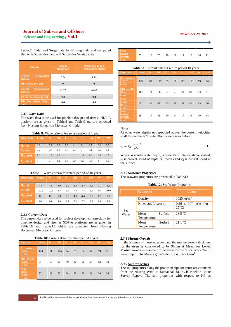
2.3.4 Tidal and Surge Data The tidal and surge data to be used for wellhead, manifold and pipeline design and riser at NDP-A platform are extracted from Nosong Bongawan Metocean Criteria. The tidal and surge data to be used for riser design at existing SUPG-B are extracted from Metocean Criteria at Sumandak Tepi and Sumandak Selatan as shown in Table.7:

ASME Description ASME VIII Div. 1 Rules of Construction of Pressure Vessel, July

2013 ASME B31.8 Gas Transmission and Distribution Piping

Systems, January 2013 ASME B16.5 Pipe Flanges and Flanged Fittings, April 2013 ASME B16.9 Factory-Made Wrought Butt Welding Fittings,

February 2013 ASME B16.20 Metallic Gasket for Pipe Flanges – Ring-Joint,

Spiral-Wound, and Jacketed, June 2013 ASME B36.10M Welded and Seamless Wrought Steel Pipe, 2010


November 29, 2013


Table.7: Tidal and Surge data for Nosong field and compared also with Sumandak Tepi and Sumandak Selatan area

Criteria Nosong Bongawan

Sumandak Tepi & Sumandak Selatan

Highest Astronomical Tide (m)

0.94 1.23

Mean Sea Level (m) 0 0

Lowest Astronomical Tide (m)

-1.17 -0.97

1 Year Storm Surge (m) 0.3 0.3

100 Year Storm Surge (m)

0.6 0.6

2.3.5 Wave Data The wave data to be used for pipeline design and riser at NDP-A platform are as given in Table.8 and Table.9 and are extracted from Nosong Bongawan Metocean Criteria.

Table.8: Wave criteria for return period of 1 year Direction Omni N NE E SE S SW W NW

Hs (m) 3.9 3.9 3.2 1.6 2 2 2.7 3.1 3.5

Tp (sec) 9.7 9.7 8.8 6.3 6.9 7 8.1 8.6 9.2

Hmax (m) 6.8 6.8 5.7 3 3.6 3.7 4.9 5.5 6.2

Tass (sec) 9 9 8.2 5.9 6.4 6.5 7.6 8 8.5

Table.9: Wave criteria for return period of 10 years Direction Omni N NE E SE S SW W NW

Hs (m) 4.6 4.6 3.9 2.0 2.4 2.4 3.3 3.7 4.2

Tp (sec) 10.6 10.6 9.7 6.9 7.6 7.7 8.9 9.4 10.0

Hmax (m) 8.1 8.1 6.8 3.6 4.3 4.4 5.9 6.5 7.3

Tass (sec) 9.8 9.8 9.0 6.4 7.1 7.2 8.3 8.8 9.3

2.3.6 Current Data The current data to be used for project development especially for pipeline design and riser at NDP-A platform are as given in Table.10 and Table.11 which are extracted from Nosong Bongawan Metocean Criteria.

Table.10: Current data for return period 1 year Direction Omni N NE E SE S SW W NW

At surface (1.0D) (cm/s)

114 71 114 74 53 64 82 74 51

Mid Depth (0.5D) (cm/s)

91 57 91 59 42 51 65 59 40

Near ottom (0.1D) (cm/s)

53 33 53 34 25 30 38 34 24

Near Seabed (0.01D) (cm/s)

25 15 25 16 11 14 18 16 11

Table.11: Current data for return period 10 years

Direction Omni N NE E SE S SW W NW

At surface (1.0D) (cm/s)

143 89 143 93 67 80 103 93 64

Mid Depth (0.5D) (cm/s)

114 71 114 74 53 64 82 74 51

Near ottom (0.1D) (cm/s)

67 42 67 43 31 37 48 43 30

Near Seabed (0.01D) (cm/s)

31 19 31 20 14 17 22 20 14

Notes: At other water depths not specified above, the current velocities shall follow the 1/7th rule. The formula is as below:

= � ∙ ��

�/� (1)

Where, � is total water depth, � is depth of interest above seabed, is current speed at depth ‘z’ metres and � is current speed at the surface

2.3.7 Seawater Properties The seawater properties are presented in Table.12

Table.12: Sea Water Properties

Parameters Values

Sea Water

Density

1025 kg/m3

Kinematic Viscosity 0.96 x 10-6 m2/s (At 25°C)

Mean Surface Temperature

28.5 ˚C

Mean Seabed Temperature

21.1 ˚C

2.3.8 Marine Growth In the absence of more accurate data, the marine growth thickness for the risers is considered to be 90mm at Mean Sea Level. Marine growth is assumed to decrease by 1mm for every 2m of water depth. The Marine growth density is 1025 kg/m3.

2.3.9 Soil Properties The soil properties along the proposed pipeline route are extracted from the Nosong WHP to Sumandak SUPG-B Pipeline Route Survey Report. The soil properties with respect to KP as


November 29, 2013


summarized below. Table.13: Nosong WHP to Sumandak SUPG-B Pipeline Route Soil Properties Kilometer

Point Drop Core

Soil Type Su (kPa)

0 - 0.5 DC-1.0 Very loose SAND with shell fragments

N/A

0.5 - 1.5 DC-2.0 Very loose SAND with shell fragments

N/A


N/A


N/A

3.5 - 4.5 DC-5.0 Very loose clayey SAND with shell fragments

N/A


N/A


N/A

6.5 - 7.5 DC-8.0 Soft grey sandy CLAY with shell fragments

14

7.5 - 8.5 DC-9.0 Very soft grey sandy CLAY with shell fragments

11

8.5 - 9.5 DC-10.0 Soft grey sandy CLAY with shell fragments

12.5


5

10.5- 11.5 DC-12.0 Very soft grey sandy CLAY with shell fragments

7


7


9


9


5


5


7


3


5


5


6


7


8


3


4


5


10


3


6

29.5 - 30.5 DC-31.0 Very soft grey sandy CLAY with sheTestll fragments

6


6


4

The soil geotechnical properties along the pipelines are taken

from Laboratory Test of Nosong WHP to Sumandak SUPG-B Pipeline Route Survey (Ref. 10) and are summarised below. Table.14: Nosong WHP to Sumandak SUPG-B Pipeline Route Soil Properties Drop Core Depth Water Content Wet Density Dry Density

(m) (%) (Mg/m3) (Mg/m3)

DC-1.0 0.8 40 1.95 1.39

DC-2.0 0.8 40 1.92 1.37

DC-3.0 0.8 40 1.92 1.37

DC-4.0 0.8 39 1.95 1.4

DC-5.0 0.72 39 1.95 1.4

DC-6.0 0.72 39 1.95 1.4

DC-7.0 0.77 37 1.95 1.42

DC-8.0 0.8 40 1.92 1.37

DC-9.0 0.3 33 1.83 1.38

DC-10.0 0.3 33 1.83 1.38

DC-11.0 0.3 35 1.83 1.36

DC-12.0 0.3 35 1.83 1.36

DC-13.0 0.4 40 2.29 1.64

DC-14.0 0.4 41 1.94 1.38

DC-15.0 0.4 32 2.03 1.54

DC-16.0 0.4 30 2.06 1.58

DC-17.0 0.4 36 2.01 1.48

DC-18.0 0.4 35 2 1.48

DC-19.0 0.4 34 2 1.49

DC-20.0 0.4 42 1.91 1.35

DC-21.0 0.2 21 1.84 1.52

DC-22.0 0.4 34 2.05 1.53


November 29, 2013


DC-23.0 0.4 46 1.91 1.31

DC-24.0 0.4 34 1.99 1.49

DC-25.0 0.4 35 1.99 1.47

DC-26.0 0.3 38 1.89 1.37

DC-27.0 0.3 38 1.7 1.23

DC-28.0 0.2 42 1.93 1.36

DC-29.0 0.4 45 1.8 1.24

DC-30.0 0.3 38 1.7 1.23

DC-31.0 0.3 38 1.7 1.23

DC-32.0 0.2 40 1.87 1.34

DC-33.0 0.2 39 1.87 1.35

3.0 SUBSEA PIPELINE ANALYSIS 3.1 Pipeline Design Parameter The pipeline design and calculation is the most crucial part in any subsea field development process. The parameters will be taken into consideration in this work are: structure of pipe, weight of pipe, design pressure and pipeline stress.

The pipeline design and operational data is based upon Pipeline Steady State Hydraulic Analysis Report and Corrosion Design Basis Memorandum is presented in Table.15. The hydrostatic test pressure shall be 1.5 times maximum allowable operating pressure / design pressure of the pipeline system or the pressure that produces hoop stress in the weakest component equal to 90% of SMYS, whichever is smaller. In the event of pig stuck during pigging operation, it is anticipated that the riser and spool at NDP-A side may be exposed to a build-up of topside pressure. Therefore, all flanges at NDP topside, riser and spool has been rated to NDP-A topside pressure and the NDP-A riser and spool has been designed to withstand NDP-A topside pressure.

Table.15: Pipeline Design and Operating Data

Parameter 10-inch FWS HP

Pipeline from NDP-A to SUPG-B

16-inch NAG LP Pipeline from

NDP-A to SUPG-B

Flow Medium FWS NAG

Min. Product Density (kg/m3) 117.68 14.64

Max. Product Density 266.68 41.49

(kg/m3)

Internal Corrosion Allowance (mm)

3 3

Corrosion Allowance for Riser Splash zone (including external) (mm)

6 6

Outside Diameter (mm) 273 406.4

Design Pressure for NDP-A Topside, Riser and Spool (bar)

186.2 186.2

Design Pressure for Subsea Pipeline, SUPG-B Topside, Riser, Spool (bar)

137.9 82.74

Hydrotest Pressure for Pipeline System (bar)

206.85 124.11

Max. Design Temperature 80 80

(°C)

Min. Design Temperature 0 0

(°C)

Maximum Operating Temperature (°C)

68 64

Pipeline and Riser Design Life (years)

25 25

Linepipe Type HFW

Material Grade for Linepipe API 5L

NDP-A Topside Rating 1500 1500

Subsea Flange Rating 1500 1500

(Note 2)

SUPG-B Topside and Pipeline System Rating

900 600

Proposed External Anti-Corrosion Coating

Above Splashzone 1mm thk. Glass Flake Filled Polyester

1mm thk. Glass Flake Filled Polyester

Riser Splashzone 12.7mm thk. Neoprene over

0.5mm thk. FBE

12.7mm thk. Neoprene over 0.5mm thk. FBE

Submerged Risers and Bends

0.5mm thk. FBE 0.5mm thk. FBE

Subsea Pipeline 5.5mm thk. AE with Concrete Weight

Coating

5.5mm thk. AE with Concrete Weight

Coating

3.2 Pipeline Material and Steel Properties The material thermal properties and densities of the pipelines and risers are shown in Table.16.

Table.16: Material Thermal Properties and Densities

Coating Type Density Thermal

Conductivity

(kg/m3) (W/m.K)

Asphalt Enamel (AE) 1280 0.69

Fusion Bonded Epoxy (FBE)

1400 0.3

3 Layer Polyethylene (3LPE)

925 0.6

3 Layer Polypropylene (3LPP)

900 0.22

Concrete Coating 3044 2.1

Carbon Steel Pipe 7850 45.35

Neoprene Coating 1450 0.265


November 29, 2013


The design will be based on the following steel material properties shown in Table.17.

Table.17: Steel Properties

Description Unit Value

Young’s Modulus, E MPa 207000

Poisson’s Ratio, - 0.3

Coefficient of Thermal Expansion 0C 11.7 x 10-6

4.0 SUBSEA STRENGTH ANALYSIS 3.1 Pipeline Design Parameter The pipeline analysis is carried out using Subsea Pro Simulation to determine wall thickness and ANSYS to determine total deformation during operation. The pipeline is subjected to internal pressure and hydrostatic pressure.

Table 18 and Figure.2 show wall thickness and stress analysis using Subsea Pro Simulation. The simulation result shows very close to the actual wall thickness.

Table.18: Actual and simulation result wall thicknesses. Actual Subsea Pro Simulation

Wall Thickness (mm) 9.525 9.130

Figure.2: Wall thickness and stress analysis using Subsea Pro Simulation.

Two types of analysis were carried out, the first is static analysis and the second is buckling analysis. The table below shows the characteristics of the pipeline.

Figure.3: Maximum Deformation (100m free span)

The analysis shows that the maximum deformation is 7.1688m at the middle of the pipeline. This analysis is carried out for 100m free span. As we can see the maximum deformation is quite high. Therefor a shorter free span is considered to decrease the maximum deformation.


The figure above shows maximum deformation for 50m free

span. As can be seen, the value is now 0.4486m only which is considerably lower than for 100m free span. The pipeline will require support on the middle of free span to offset the buckling load.


The figure above shows maximum deformation for 10m free


November 29, 2013


span. The maximum value is 0.0008 m which is almost zero. This proves that the shorter the free span, the smaller the static deformation. However, selecting the optimum free span must include other factor such as cost and efficiency. 5.0 CONCLUSION In conclusion, this paper discussed subsea pipeline of Nosong-Bongawan field development, Malaysia. Wall thickness and stress of the subsea pipeline were analyzed using Subsea Pro Simulation and ANSYS. The simulation result shows the simulation result was very close to the actual wall thickness. ACKNOWLEDGEMENTS The authors would like to convey a great appreciation to Universiti Teknologi Malaysia and Ocean and Aerospace Engineering Research Institute, Indonesia for supporting this research. REFERENCES 1. Abdul Khair Junaidi, and Jaswar Koto, 2015, Initial

Imperfection Design of Subsea Pipeline to Response Buckling Load, Journal of Ocean, Mechanical and Aerospace -Science and Engineering-, Vol. 15, pp.7-11.

2. Abdul Khair Junaidi, Jaswar Koto, 2014, Parameters Study of Deep Water Subsea Pipeline Selection. UTM Press.

3. Abdul Khair Junaidi, Jaswar Koto, 2014, Parameters Study of Deep Water Subsea Pipeline Selection, Jurnal Teknologi, Vol 69, No 7, pp.115-119.

4. Abdul Khair, J., Jaswar, Koto, Affis Effendi, Ahmad Fitriadhy, 2015, Buckling Criteria for Subsea Pipeline, Jurnal Teknologi, Vol 74, No 5, pp.69-72.

5. ASME B16.5, 2013, Pipe Flanges and Flanged Fittings. 6. DNV RP E305, 1988, On-Bottom Stability Design of

Submarine Pipelines. 7. DNV RP F103, 2010, Cathodic Protection of Submarine

Pipelines by Galvanic Anodes. 8. DNV, 1981, Rules for Submarine Pipeline Systems. 9. Harun Al-Rashid Bin Azmi, 2013, Conceptual Design for

Deep Water Pipeline, Faculty of Mechanical Engineering, Universiti Teknologi Malaysia.

10. ISO 15589-2, 2007, Petroleum and Natural Gas Industries, Cathodic Protection of Pipeline Transportation Systems Part 2: Offshore Pipelines.

11. J.Koto, A.K. Junaidi, 2016, Subsea Pipeline Design & Analysis, Second Edition, Ocean & Aerospace Research Institute, Indonesia & Universiti Teknologi Malaysia.

12. PETRONAS Technical Standard, PTS 30.10.73.34, 2012, Design of Cathodic Protection Systems for Offshore Pipelines (Amendments/Supplements to DNV RP F103).

13. PETRONAS Technical Standard, PTS 31.40.00.20, 2012, Pipeline and Riser Engineering.


June 30, 2016


The Effect of Flat Plate Theory Assumption in Post-Stall Lift and Drag Coefficients Extrapolation with Viterna Method

Faisal Mahmuddina,*

a)Marine Engineering Department, Engineering Faculty, Hasanuddin University, Makassar Indonesia *Corresponding author: [email protected] Paper History Received: 25-June-2016 Received in revised form: 28-June-2016 Accepted: 30-June-2016

ABSTRACT In employing blade element momentum (BEM) method to compute the performance of a turbine propeller, the lift and drag coefficients of propeller element/airfoil are needed. The coefficients are usually obtained from model experiment. Unfortunately, the model experiment can only be conducted for small angle of attack until stall mode. Beyond stall mode, Viterna extrapolation method is commonly used. The method is used to predict the lift and drag coefficients from stall angle to 90o. Beyond that range, besides Viterna method, original flat plate theory assumption can also be adopted. The present study compares the lift and drag coefficients extrapolation using Viterna method and flat plat theory. NACA2415 airfoil shape is used for computation. The computation formulas and procedures are presented and important parameter effect to the coefficients are shown and explained. KEY WORDS: Blade Element Momentum, Experimental Data Extrapolation, Flat Plate Theory, Lift and Drag Coefficients, NACA2415, Viterna Method. NOMENCLATURE

AR aspect ratio AoA angle of Attack CD drag coefficient CL lift coefficient

α angle of attack 1.0 INTRODUCTION One of popular methods to predict the power produced by a wind turbine is blade element momentum (BEM) method. The main advantages of the method are simple formulation, fast computation, and good accuracy results especially for steady state condition. Examples of BEM method application can be found in references (Ceyhan, 2008; Døssing, Madsen, & Bak, 2011; Godreau, Caldeira, & Campos, n.d.; Liu & Janajreh, 2012).

In this method, the propeller blade is divided into several elements/airfoil. Each element is assumed to act independently and has no interaction between them. The forces and moments are computed on each element/airfoil. The total forces and moments are obtained by integrating the forces and moments on each element/airfoil.

Therefore, in order to use the BEM method, each element/airfoil performance in terms of lift and drag coefficients is necessary. The performance is usually obtained by conducting a model experiment. However, the model experiments can only be conducted for small angle of attack (AoA) until stall mode. For post stall mode performance, it necessary to extrapolate the data obtained from the model experiment in order to obtain the full 360o data.

For obtaining the full polar data, several extrapolation methods can be used such as Bean and Jakubowski correlation, Kirke Correlation, Montgomerie model, Viterna model, etc. (Bianchini et al., 2016). Of the methods, Viterna model is the most common one to be used because it can be implemented more straightforwardly with reliable results.

The Viterna method is used specifically to be implemented to predict the lift and drag coefficients from stall mode to 90o of AoA. For AoA higher than 90o, formulation based on the original flat plate theory can also be implemented.

The present study compares the data extrapolation results computed using Viterna method and original flat plate theory. The computation formulas and procedures of both


June 30, 2016


implementation methods are presented and important parameter effect to coefficients are shown and explained. For demonstrating the calculation procedures, an airfoil based on NACA2415 shape is used. 2.0 SOLUTION METHOD In the present study, the Viterna method is used to extrapolate the lift and drag coefficients beyond the stall angle until 90o. Beyond that range, original flat plate theory assumption can also be adopted. 2.1 Viterna Method The Viterna method, also known as Viterna-Corrigan method, is a data extrapolation method for AoA (α) greater than stall angle (αstall) but less than or equal to 90o. The method was formulated by utilizing flat plate theory (Matthew, 2009). It requires an initial angle with its associated drag and lift coefficients which should satisfy flat plate theory.

The Viterna method is formulated to extrapolate the lift and drag coefficients using the following equation (L. A. Viterna & Janetzke, 1982; L. Viterna & Corrigan, 1982):

2

1 2

cossin

s2

inL AC Aαα

α+= (1)

21 2sin cosDC B Bα α+= (2)

where

1 2

maxDCA = (3)

1 maxDB C= (4) ( )2 2

sinsin cos

cosstall max stall stastal

llstall

lL DA C C

αα αα

= − (5)

2

2

sin

cosstall maxD stall

tall

D

s

CCB

αα

=−

(6)

CDmax is found using aspect ratio (AR) as follows

1.11 0.018maxDC AR+� (7)

The AR in Eq. (7) can be obtained from BEM method

application where finite blade length will affects the flat plate assumption. The chosen value of AR will not affect the results significantly. AR equals to 9-10 can be used for most computations.

For data extrapolation from α > 90o to α < αmin, the calculated values are reflected. The Viterna method does not consider pressure or skin friction distributions; however, by making a few simple assumptions and correction, it is possible to obtain a reasonable estimate from the Viterna method. While the method is not an accurate representation of the true physics, it provides a reasonable estimate and accuracy in early design process.

2.2 Flat Plate Theory It is known from flat plate theory that for deep stall or high angle of attack region (greater than 20o), the upper surface of the airfoil receives no direct impact from the flow due to flow separation. The condition is consistent with what so-called Newtonian Flow condition. Consequently, the thickness of the airfoil can be neglected. In this deep stall region, lift and drag coefficients are largely independent of airfoil geometry but mainly depends on the blade geometry and aspect ratio (J. L. Tangler, 2004).

Moreover, the flow of lower surface is completely laminar, and its contribution to the overall drag force is very small. Therefore, when the foil in high angle of attack position, the foil will behave like a thin of flat plate.

When assuming that the airfoil behave like a flat plate for deep stall angle, the flow separation effect will exist. Therefore, in order to resolve the flat plate flow behaviour, the stagnation point on the rear side of the airfoil is moved by assuming potential flow theory like behaviour. Based on the principle, the curve of lift and drag coefficients can be described using the following equations (Duquette, 2007; J. Tangler & Kocurek, 2005; Timmer, 2010).

2sin cosLC α α= (8)

22sinDC α= (9)

It can be implied from Eq. (8) and (9) that lift and drag coefficients at α = 0 will be zero. This is idealization of the curve and not realistic. Even though not realistic, the theory assumption was found to be a good first-order approximation of lift and drag coefficients (Hoburg & Tedrake, 2009). 2.2 4 (four) Digits NACA Airfoil In 1930, NACA (National Advisory Committee for Aeronautics) – the frontrunner of NASA (National Aeronautics and Space Administration) – conducted airfoil experiments using rational and systematic shapes. Based on the shapes, NACA established the shape nomenclature which is now a well-known standard (Tobergte & Curtis, 2013).

Original NACA airfoil series consists the 4-digit, 5-digit, and modified 4-/5-digit which can be drawn using analytical equations that involve the camber (curvature) of the mean-line (geometric centreline) of the airfoil section as well as the section's thickness distribution along the airfoil length. Later series has included the 6-digit series which are more complicated shapes constructed using theoretical rather than geometrical methods.

The 4-digit series are first family of NACA series airfoil. The first digit specifies the maximum camber (m) in percentage of the chord (c), the second indicates the position of the maximum camber (p) in tenths of chord, and the last two digits provide the maximum thickness (t) of the airfoil in percentage of chord. For example, the NACA2415 airfoil, which is the one used in the present study, means the airfoil has a maximum thickness of 15% (0.15c) with a camber of 2% (0.02c) located 40% (0.4c) back from the airfoil leading edge. By knowing the values of m, p, and t, the coordinates and shape of an airfoil can be computed and drawn.


June 30, 2016


3.0 AIRFOIL DATA The computed airfoil shape in the present study is NACA2415. Using the definition of 4 (four) digits NACA airfoil described in the previous section, the shape of the airfoil is drawn and shown in the following figure

Figure 1: NACA2415 airfoil shape

The lift and drag coefficients of the airfoil will be the input data for the program code. The coefficients of the airfoil will be mostly taken from experiment data which can be found in reference (Abbott & Doenhoff, 1949). The experimental results are shown in the following graphs.

(a) NACA2415 Lift coefficient

(b) NACA2415 Drag coefficient

Figure 2: NACA2415 Lift and Drag Coefficients (Abbott & Doenhoff, 1949)

However, it can be seen from Fig. 2 that after AoA of 15.95o,

the CD cannot be determined from experimental graph. Therefore, in order to resolve the issue, a polynomial fit will be used to predict the value of CD for this range. The same procedure has also been demonstrated in reference (McCosker, 2012).

For the present case, 3rd order polynomial is used to predict the CD for unknown CD range. By using the available data, the equation of the polynomial can be determined and shown as 3 5 27 58 10 4 10 6 10 0.0063x x x−− −⋅ + ⋅ + ⋅ + (10)

The summary of CL and CD data obtained from experiment

curve and predicted by Eq. (10) are shown in the following table

Table 1: NACA2415 Lift and drag coefficients AoA (degree) CL CD

-10.34 -0.86 0.00905 -8.27 -0.64 0.00786 -6.2 -0.42 0.00718 -4.34 -0.24 0.00676 -2.27 -0.02 0.00647 -0.2 0.2 0.00648

0 0.2 0.4 0.6 0.8 1

NACA Parametersm= 0.02c t = 0.15cp = 0.4c


June 30, 2016


1.87 0.41 0.00651 3.94 0.61 0.00699 5.59 0.84 0.00799 7.66 1.06 0.00935 9.73 1.27 0.01116 11.8 1.43 0.01368 13.66 1.57 0.01613 15.95 1.65 0.019722 18.03 1.59 0.023992 20.12 1.34 0.029008 22.2 1.25 0.034766 24.27 1.34 0.041298

In order to observe more clearly the input data, the data

shown in the above table is shown in graph below.

Figure 3: Experimental and predicted CD and CL

As shown in the above graph, stall angle is around 15o of AoA.

Unfortunately, as described before, the CD data are not available for post-stall angle. Therefore, they are predicted using polynomial equation shown in Eq. (10). The predicted CD data are shown as green circle symbol in Fig. 3.

4.0 RESULTS AND DISCUSSION Based on the airfoil CD and CL coefficients shown in Table. 1, computations are performed using the methods described in the preceding section. The first computation is performed to analyse the effect of Coefficient lift adjustment (CLadj) to lift coefficient. The CLadj is an important parameter needs to be determined when using the Viterna method to predict the lift and drag coefficients beyond the range from stall angle to 90o. CLadj will determine the maximum value of computed CL.

3 (three) values of CLadj are used which are CLadj = 0.7, 0.9, and 1.2. The computation results are shown in the following figure

Figure 4: Effect of CLadj to lift coefficient

From figure, it can be seen that CLadj = 0.9 has the best fit to

the line compared to other values of CLadj. Therefore, the next computation will use CLadj = 0.9.

The next computation is performed to analyse the extrapolation of CL using Viterna method only and flat plate theory assumption. The computation results are shown in the following figure

Figure 5: Lift coefficients comparison

It can be observed from the figure that there are discrepancies

of results around the peak which are around -170o and 170o. Higher peak can be resolved by implementing flat plate theory assumption as shown as red line. As a result, from the figure, it can also be noted the shape is much more sinusoidal when applying the original flat plate theory assumption. The assumption is used in computing lift and drag coefficients from 90o to 180o and in its reflection in negative side of the curve.

The results for drag coefficients are shown in the following figure

AoA (degree)

Lif

tCoe

ffic

ien

t(C

L)

Dra

gC

oeff

icie

nt(C

D)

-15 -10 -5 0 5 10 15 20 25-1

-0.5

0

0.5

1

1.5

2

0

0.005

0.01

0.015

0.02

0.025

0.03

0.035

0.04

0.045

0.05

CLCD ExperimentCD Prediction

AoA

CL

-180 -120 -60 0 60 120 180

-1.5

-1

-0.5

0

0.5

1

1.5

Viterna and Flat PlateViterna Only CLadj=0.7Viterna Only CLadj=0.9Viterna Only CLadj=1.2

AoA (degree)

Lif

tCoe

ffic

ient

(CL

)

-180 -120 -60 0 60 120 180

-1.5

-1

-0.5

0

0.5

1

1.5

Viterna Method OnlyViterna & Flat Plate TheoryExperimental Data


June 30, 2016


Figure 6: Drag coefficients comparison

From figure above, it can be observed a good agreement

between Viterna method and flat plate theory assumption in in terms of shape and magnitude of the curve. The results show that the effect of Viterna method for CD extrapolation is not significant. Significantly higher CDmax in the curve can be adjusted using the value of AR as shown in Eq. (7). 5.0 CONCLUSION In the present study, implementation of lift and drag coefficients experimental data extrapolation using Viterna method and flat plate and theory assumption are performed. It is found that discrepancies can be noticed for lift coefficients while a good agreement can be found in terms of shape and magnitude for drag coefficient. The computation results shown in the present study will be important for determining the Viterna method implementation procedure when using blade element momentum (BEM) method. ACKNOWLEDGEMENTS This work was supported by Unggulan Perguruan Tinggi (UPT) research grant from Indonesian Directorate General of Higher Education and Hasanuddin University, Makassar for fiscal year 2016. REFERENCE 1. Abbott, I. H., and Doenhoff, A. E. V. (1949). Theory of Wing

Sections Including a Summary of Airfoil Data. New York: Dover Publication, Inc.

2. Bianchini, A., Balduzzi, F., Rainbird, J. M., Peiro, J., Graham, J. M. R., Ferrara, G., and Ferrari, L. (2016). An Experimental and Numerical Assessment of Airfoil Polars for Use in Darrieus Wind Turbines — Part II : Post-stall Data Extrapolation Methods. Journal of Engineering for Gas Turbines and Power, Vol. 138(3), pp: 1–10.

http://doi.org/10.1115/1.4031270 3. Ceyhan, O. (2008). Aerodynamic Design and Optimization of

Horizontal Axis Wind Turbines by Using BEM Theory and Genetic Algorithm. Middle East Technical University.

4. Døssing, M., Madsen, H. A., and Bak, C. (2011). Aerodynamic Optimization of Wind Turbine Rotors using a Blade Element Momentum Method with Corrections for Wake Rotation and Expansion. Wind Energy, Vol. 15(4), pp: 563–574. http://doi.org/10.1002/we

5. Duquette, M. M. (2007). The Development and Application of SimpleFlight , a Variable-Fidelity Flight Dynamics Model. In AIAA Modeling and Simulation Technologies Conference and Exhibit.

6. Godreau, C., Caldeira, J., and Campos, J. A. C. F. De. (n.d.). Application of Blade Element Momentum Theory to the Analysis of a Horizontal Axis Wind Turbine. In V Conferência Nacional de Mecânica dos Fluidos, Termodinâmica e Energia (MEFTE). Porto, Portugal.

7. Hoburg, W., and Tedrake, R. (2009). System Identification of Post Stall Aerodynamics for UAV Perching. In AIAA Infotech@Aerospace Conference. Seattle, Washington.

8. Liu, S., and Janajreh, I. (2012). Development and Application of an Improved Blade Element Momentum Method Model on Horizontal Axis Wind Turbines. International Journal of Energy and Environmental Engineering, Vol. 3(30), pp: 1–10.

9. Matthew, A. B. (2009). A Computational Method for Determining Distributed Aerodynamic Loads on Planforms of Arbitrary Shape in Compressible Subsonic Flow. University of Kansas.

10. McCosker, J. (2012). Design and Optimization of a Small Wind Turbine. Rensselaer Polytechnic Institute.

11. Tangler, J., and Kocurek, J. D. (2005). Wind Turbine Post-Stall Airfoil Performance Characteristics Guidelines for Blade-Element Momentum Methods. In 43rd AIAA Aerospace Sciences Meeting and Exhibit.

12. Tangler, J. L. (2004). Insight into Wind Turbine Stall and Post-stall Aerodynamics. Wind Energy, Vol. 7, pp: 247–260. http://doi.org/10.1002/we.122

13. Timmer, W. A. (2010). Aerodynamic Characteristics of Wind Turbine Blade Airfoils at High Angles-of-Attack. In TORQUE 2010: The Science of Making Torque from Wind. Crete, Greece.

14. Tobergte, D. R., and Curtis, S. (2013). Fundamental of Aerodynamics. Journal of Chemical Information and Modeling, Vol. 53(9), pp: 1689–1699. http://doi.org/10.1017/CBO9781107415324.004

15. Viterna, L. A., and Janetzke, D. C. (1982). Theoretical and Experimental Power From Large HorizontaI Axis Wind Turbines (Vol. 82944). Cleveland, Ohio.

16. Viterna, L., and Corrigan, R. (1982). Fixed Pitch Rotor Performance of Large Horizontal Axis Wind Turbines. In DOE/NASA Workshop on Large Horizontal Axis Wind Turbines, Cleveland.

AoA (degree)

Dra

gC

oeff

icie

nt(

CL

)

-180 -120 -60 0 60 120 1800

0.5

1

1.5

Viterna Method OnlyViterna & Flat Plate TheoryExperimental Data


June 30, 2016


Review on Roncador Field Production and Gas Lift Pipelines

Adibah Fatihah.M.Y,a, Noor Zairie. M,a, Nur Ain. A.R,a, Nursahliza. M.Y,a and J.Koto,a,b,*

a) Department of Aeronautic, Automotive and Ocean Engineering, Faculty of Mechanical Engineering, Universiti Teknologi Malaysia b) Ocean and Aerospace Engineering Research Institute, Indonesia *Corresponding author: [email protected] and [email protected] Paper History Received: 5-June-2016 Received in revised form: 27-June-2016 Accepted: 30-June-2016

ABSTRACT The production of oil and gas in Brazil is keeping going as long as there is demand worldwide, same for the development of subsea system technology. The Roncador Field has been leading the technological challenges of Petrobras in ultra-deep water -1500 to 1900 meters- which covers an area of approximately 110 square kilometers. This paper discussed pressures and stress of subsea pipelines on Roncador Field using Subsea Pro Simulation to analyze the wall thickness and ANSYS to analyze the stress distribution along the pipe. KEY WORDS: Roncador Field, Wall Thickness, Subsea Pipeline, Stress. NOMENCLATURE

BBLD Billion Barrels per Day OD Outside Diameter ID Inside Diameter �� Wall Thickness �� Million Metric Standard Cubic Meter Per Day �� Floating Production Unit �� Early Production Riser 1.0 RONCADOR FIELD

Campos Basin is located on offshore Rio de Janeiro State, which is on the Southeast region of Brazil. The Campos basin covers area of 100 square km ranging from 20 m to 3,400 m water depth. After Petrobras discovered 2 giant fields in Campos Basin, Albacora, 1984 and Marlim, 1985 in water depth 200 m to 2000 m, they faced 11 years later (1996) to the discovery of Roncador Field in water depth ranging from 1,500 m to 1,900 m. Roncador Field is a giant field located in the northern area of Campos Basin as shown in Figure.1.

Figure.1: Maps of Campos Basin and Roncador Field [Offshore Energy].

The Roncador Field has been leading the technological challenges of Petrobras in ultra-deep water since it is discovery. It has the world's first drill pipe riser, subsea tree and Early Production Riser (EPR) rated 2,000m. The first well in Roncador is RJS-436A connected to the FPSO Seillean from 1999 to 2001 using EPR at water depth 1,853m with GLL TLD 2000 subsea tree. This field has 3 billion barrels of proven recoverable oil reserves. Due to its large reservoir size, the field was divided into four modules, Module 1 has oil well 28-31 API, Module 2 oil


June 30, 2016


wells 18 API, Module 3 has oil well 22 API and Module 4 has oil well 18 API. Module 1 has two phases, Phase 1 and Phase 1A. There are total 94 wells in Roncador Field, which is 60 wells are production well and 34 wells are water injection wells. Two types of subsea technologies were used; vertical and horizontal. Both tree technologies are guide-lineless with vertical flow-line connection with individual vertical modules. Several offshore floating structures have been chosen to operate in Roncador Field for production activity such as floating production storage and offloading vessels and semi-submersibles. 2.0 RONCADOR FIELD PROJECT DEVELOPMENT Petrobras developed Roncador field in four modules because of its large size and different oil gravity in each area. Module 1 has several phases. Figure.2 shows the project development modules in Roncador Field.

Figure.2: Project Development Modules in Roncador Field [Henrique.at.al, 2013].

The Early Production Phase started producing in 1999 from the first well, RJS-436. This well located at water depth 1,853 m and connected to FPSO Seillean. This phase was set to produce early in order to create revenue for the project to cover the huge costs for development the whole field. During this phase, the production was 20,000 BBLD.

Phase one of Module 1 consisted of several wells connected to semi-submersible production facility P-36. It is start producing in 2000 and later in March 15, 2001, this semi-submersible has sunk due to explosions due to human error. During that time, P-36 is considered the biggest submersible which produced 84,000 BBLD of oil and 1.3MMscmd of processing gas. After the P-36 incident, Petrobras has started with Module 1A: Phase One. They want the field to producing as soon as possible. FPSO Brasil has been installed on water depth 1,290 m and eight production wells have been connected to the vessel. On 2002, the field has started production again.

In Module 1A Phase Two, new build semi-submersible P-52 has been fabricated and installed in 2007. This platform is connected to 18 subsea production wells and 11 water injection wells. The submersible produce 20,000 BBLD peaking to

180,000 in second-part of 2008. The peak gas produced from this phase was 3.2 MMSCMD. For this project, we will focus on Module 1A only. A module 2 development consists of 17 long horizontal wells which 11 of them are production wells and 6 are water injection wells. FPSO P-54 has been assigned for production in this module and started operation in 2007. This phase has helped to boost the overall production from the field to 460,000 BBLD. Development of module 3 consists of 11 add-on production wells and 7 water injection wells. For this module, semi-submersible P-55 has been assigned for production. The production capacity for this platform is 180,000 BBLD and gas compression capacity is 6 MMSCMD. The platform started its production in 2013. Module 4 development consists of 19 wells, which is 12 wells are production well and another 7 wells are water injection well. An FPSO P-62 has been assigned for this module. This FPSO is a cloned to the P-54 FPSO. The production capacity is 180,000 BBLD and gas compression capacity is 6 MMSCMD. This platform started its production in 2014. 3.0 RONCADOR TRANSPORTATION SYSTEM The module 1A of the Roncador field, offshore Brazil, has been developed employing a large production semi-submersible unit. The integrated gathering system of phase-2 as in Figure.3 involved subseas wellheads and manifold in water depth varying from 1550 to 1900 meters. The production and injection flowlines systems connect the FPU directly to each well, meanwhile the well gas lift flowlines are attached to three subsea manifolds linked to P-52 through a Gas Lift “Ring” pipeline. All flowlines and risers for integrated gathering system are currently both rigid and flexible pipes. Subsea connection flowlines on wellheads and manifolds also were provided by flexible pipe or known as Vertical Connection Module.

Figure.3: Overview of Roncador subsea system [Claudio, 2014].

These flowlines networks to connect to 18 production wells, 11 water injection wells, 4 spare wells and three manifolds (Jose et al., 2006) consists of 335 km of flexible flowlines for gas and production pipelines and 60 km of rigid pipelines for production and gas lift pipelines. The details for production and gas lift flowline for the respected system as in Table.1.


June 30, 2016


Table.1: Production and gas lift flowlines details [Morais et al, 2001].

Particular Length

(m)

Pipe Diameter

(Inch)

Production pipeline

Insulated flexible jumper 120 6

from wellhead

Insulated steel flowline

with

8000 6

PLET's in both ends

Insulated flexible flowline 1100 6

Flexible riser to platform 1720 6

Gas lift Pipeline

Flexible jumper from 120 4

wellhead

Steel flowlines with 8000 4

PLETs in both end

Flexible flowline 1100 4

Flexible riser to platform 1720 4

In addition, Figure.4 discussed the typical composition of the

flowlines which connecting the wellhead to the FPU [Azevedo et al., 2001] consists of:

1. Pull in head 2. Flange 3. Riser 4. Extension Flowline 5. Isolation Valve 6. VCM 7. PLET 8. Steel Pipeline 9. Flexible Jumper 10. VCM on Wellhead

Figure.4: Composition of Flowline [Azevedo et al., 2001].

The production flowlines based on API 5LX60 were coated

with fusion-bonded epoxy (FBE) and thermal insulation coating wrapped-solid polypropylene. Gas-lift pipelines based on API 5LX60 were coated FBE-polyethylene for corrosion and mechanical damage protection (single pipeline insulation coating) as in the Table.2: The properties of insulation coating for production pipeline can be described in the Table.3.

Table.2: Roncador Rigid Pipeline Data [Marcos et al., 2001]

Pipeline Type Cross Section

Description of Steel Coating

Steel OD WT ID OD/WT FBE Adhesive Insulation Shield

(mm) (mm) (mm) (mm) (mm) (mm) (mm) (mm)

6 inch production line X60 177.8 14.3 149.3 12.5 0.1 0.4 60 0

4 inch gas lift line X60 141.3 12.7 115.9 11.1 0.1 0.3 0 5

Table.3: Roncador Production Pipeline Insulation Data [Marcos et al., 2001].

No. Product Nominal Thickness (mm)

Thermal Conductivity

W/mᵒK

1 Solid Polypropylene

60 0.22

3.0 SUBSEA PIPELINE SIMULATION 3.1 Subsea Production Pipeline Rocandor field use type single pipe with coating for production pipelines. The pipe consists inside pipe, coating and insulation. Below is the calculation for production pipeline. The pipelines data used in the calculation are shown in Tables.4 - 8.


June 30, 2016


Table.4: Rigid Pipeline Data

Parameter Unit Value

Outside Diameter, D mm 177.8

Wall thickness, t mm 14.3

Pipe material grade - X60

• Steel Density, ρst Kg/m3 7850

• Specified Minimum Yield

Strength, (SMYS)

Mpa 413

• Specified Minimum Tensile

Strength, (SMTS)

MPa 517

• Poisson ratio (ν) - 0.3

Young's Modulus, E Gpa 207

Thermal Expansion Coefficient (α) C-1 1.17x10-5

Table.5: Insulation and Coating Data


Insulation Thickness, tcr m 0.0001

Insulation Density, ρcr Kg/m3 1300

Concrete Coating Thickness, tcn m 0.060

Concrete Coating Density,ρcn Kg/m3 912.2

Table.6: Operating Data


Content Oil density, ρcn Kg/m3 897

Design Internal Pressure, Pi Mpa 30

Operating Temperature, To oC 67

Table.7: Environmental data


Seawater density Kg/m3 1027

Water Depth m 1870

External Pressure (Pe) Mpa 18

Ambient Temperature, Ta oC 5

Friction factor - 0.58

Table.8: Soil data

PARAMETER VALUE

Axial Friction 0.5

Lateral Friction LB 0.3

BE 0.5

UB 0.7

Soil Mobilization 2mm-4mm

The limit state of hydrostatic test pressure can be formulated as follows:

�� . �� . �� . �� (1) Where; �� is burst design factor of internal pressure 0.90 for pipeline and 0.75 for riser, �� is joint factor of weld and �� is Temperature derating factor.

Figure.5 shows subsea pipeline stress analysis using Subsea Pro Simulation. The Subsea Pro indicated that the minimum acceptable wall thickness is 14.30 mm for 50 target years. The internal pressure is more dominant at this water depth.


June 30, 2016


Figure.5: Subsea Production Pipeline Stress analysis using Subsea Pro Simulation.

3.2 Subsea Gas Lift Pipeline Rocandor field use type single pipe with coating for production gas lift pipelines. The pipe consists inside pipe, coating and insulation. Below is the calculation for gas lift pipeline. The pipelines data are shown in Tables 9 - 11.

Table.9: Rigid Pipeline Data

PARAMETER UNIT VALUE

Outside Diameter, D mm 141.3

Wall thickness, t mm 12.7

Pipe material grade - X60

• Steel Density, ρst Kg/m3 7850

• Specified Minimum Yield

Strength, (SMYS)

Mpa 413

• Specified Minimum Tensile

Strength, (SMTS)

MPa 517

• Poisson ratio (ν) - 0.3

Young's Modulus, E Gpa 207

Thermal Expansion Coefficient (α) C-1 1.17x10-5

Table.10: Insulation and coating Data


Insulation Thickness, tcr m 0.0001

Insulation Density, ρcr Kg/m3 1300

Concrete Coating Thickness, tcn m 0.005

Concrete Coating Density,ρcn Kg/m3 3040

Table.11: Operating Data


Content Gas density, ρcn Kg/m3 0.668

Design Internal Pressure, Pi Mpa 30.00

Operating Temperature, To oC 67

Subsea gas lift pipeline stress analysis was done using Subsea Pro Simulation as show in Figure.6. The Subsea Pro indicated that the minimum acceptable wall thickness is 12.43 mm for 50 target years. The internal pressure is more dominant at this water depth.


June 30, 2016


Figure.6: Subsea Gas Lift Pipeline Stress analysis using Subsea Pro Simulation 4.0 FINITE ELEMENT ANALYSIS Finite element method is a numerical procedure to obtain verification and engineering solutions. The aim for this analysis is to access the structural behaviour of the pipe under loading condition. For this analysis, ANSYS Workbench Static Structural Analysis has been used based on available operating data. 4.1 Load and boundary conditions In this study, the pipe model is built by ANSYS 14 according to the scale to define stress and strain during normal operation in different water depth level of 1800 meters. The pipe has total length of 120 m and the material properties are correspond to API 5L. The internal pressure of 22 MPa and external pressure of 18 MPa are applied and the wall thickness and outer diameter of pipe for production line are 14.3 mm and 177.8 mm respectively, meanwhile the wall thickness and outer diameter for gas line are 12.7 mm and 141.3 mm respectively (details of the operating condition can be refer at previous section). The both ends of the pipeline are fixed as restraint condition and the simulation is running without pipeline coating. 4.2 Equivalent stress, strain and buckling for production pipeline Figure.5 illustrates the equivalent stress in elastic model without concrete coating by using static structure analysis of ANSYS for production pipe. The maximum stress is 190 MPa while the minimum stress is 79 MPa. The equivalent strain is illustrated by Figure.6 which the maximum 9.6313e-4 and the minimum strain will be 4.7654e-4. Figure.7 show the pipeline buckling for production line which is the maximum deformation is 1.0326 m.

Figure.5: Equivalent stress for production pipeline

Figure.6: Equivalent strain for production pipeline

Figure.7: Production Pipeline Buckling In ANSYS Configuration

4.3 Equivalent stress, strain and buckling for gas pipeline

Figure.8 illustrates the equivalent stress in elastic model without concrete coating by using static structure analysis of ANSYS for gas pipeline. The maximum stress is 170 MPa while the minimum stress is 80 MPa. The equivalent strain is illustrated by Figure.9 which the maximum 9.093e-4 and the minimum strain will be 5.244e-4. Figure.10 show the pipeline buckling for production line which is the maximum deformation is 1.0024 m.

Figure.8: Equivalent stress for gas pipeline


June 30, 2016


Figure.9: Equivalent strain for production pipeline

Figure.10: Gas Pipeline Buckling In ANSYS Configuration 5.0 CONCLUSION In conclusion, this paper discussed on wall thickness and stress of subsea production and gas lift pipelines in Roncador Field, Brasil. Wall thicknesses of the pipelines were investigated using Subsea Pro Simulation and equivalent stress, strain and buckling were analyzed using ANSYS software. ACKNOWLEDGEMENTS The authors would like to convey a great appreciation to Universiti Teknologi Malaysia, Malaysia and Ocean and Aerospace Engineering Research Institute, Indonesia for supporting this research. REFERENCE 1. Abdul Khair Junaidi, and Jaswar Koto, 2015, Initial

Imperfection Design of Subsea Pipeline to Response Buckling Load, Journal of Ocean, Mechanical and Aerospace -Science and Engineering-, Vol. 15, pp.7-11.

2. Abdul Khair Junaidi, Jaswar Koto, 2014, Parameters Study of Deep Water Subsea Pipeline Selection, Jurnal Teknologi, Vol 69, No 7, pp.115-119.

3. Abdul Khair, J., Jaswar, Koto, Affis Effendi, Ahmad Fitriadhy, 2015, Buckling Criteria for Subsea Pipeline, Jurnal Teknologi, Vol 74, No 5, pp.69-72.

4. Bai, Y., & Bai, Q. (2012). Subsea engineering handbook: Gulf Professional Publishing.

5. Bordieri, E., Barbosa V. C., Dias, R, 2008, An Overview of the Roncador Field Development, a Case in Petrobras Deep Water Production, Offshore Technology Conference, 5-8 May, Houston, Texas, USA

6. Claudio Paschoa, 2014, Brazil Offshore: Petrobras &

Subsea Engineering, Maritime Professional. 7. De Gam Lima, J. M. T., Kuppens, M. L., da Silveira, P. F.,

and Stock, P. F. K, 2008, Development of Subsea Facilities in the Roncador Field (P-52), Offshore Technology Conference, pp. 72 – 75.

8. E. Neto and J. Mauricio, Petrobras S/A and I. Wacleawek, CSO Brazil, 2001, Flexible Pipe for Ultra- Deepwater Applications: The Roncador Experience. “Offshore Technology Conference, Houstan, Texas”

9. F.B Azevedo, Petrobras, M. J. B Teixeira, Petrobras, G. Portesan, Soco-Ril, M. Kalman, Garcia, A. L., Pinto, F. J., Dias, M. A., & Mattos, A. M, 1998, Roncador Field-A Rapid Development Challenge in Ultra-Deep Water, Offshore Technology Conference, Houstan, Texas.USA.

10. Henrique Peres Moro, Gustavo da Cunha Maia, Daniel Henriques Mesquita Lage and Eduardo Bordieri, 2013, Roncador Module IV: A Successful Case of Heavy Oil Projects in Ultra deep waters, Offshore Technology Conference, Brasil.

11. J.Koto, A.K. Junaidi, 2016, Subsea Pipeline Design & Analysis, Second Edition, Ocean & Aerospace Research Institute, Indonesia & Universiti Teknologi Malaysia.

12. J.R.F. Moreira and T.E. Johansen (2001). Installation of Subsea Trees in Roncador Field, at 1800m Water Depth Using the Drill Pipe Riser, Offshore Technology Conference, Houstan, Texas.

13. Jaswar, Abdul Khair, J., H. A. Rashid. 2013. Expansion of Deep Water Subsea Pipeline, The International Conference on Marine Safety and Environment, Malaysia

14. Jaswar, Abdul Khair, J., Hashif. 2013. Effect of Axial Force Concept in Offshore Pipeline Design. The International Conference on Marine Safety and Environment, Malaysia

15. Jose Mauricio T.G Lima, Mariele Lima Kuppens, Paulo Frreira da Silviera, and Pedro Felipe K. Stock, Petrobras (2008). Development of Subsea Facilities in the Roncador Field (P-52). “Offshore Technology Conference Houstan, Texas”, OTC 19274

16. Juiniti, R, 2001, Roncador Field Development with Subsea Completions, . Conference on Ocean Offshore and Arctic

Engineering, Houston, Texas, pp.1-8. 17. Keppens, M. L., Batista da Silva, J. L., Ribeiro Contarini, M.

G., Pereira Pinto, F. J. C. (2006). Roncador Field Subsea Manifold: A Risk Analysis Approach to Verify the New Installation Procedure. Conference on Ocean Offshore and Arctic Engineering

18. Koto, J and Junaidi, A.K, 2016, Subsaa Pipeline Desing & Analysis, Second Idition, Ocean & Aerospace Research Institute, Indonesia.

19. L.P. Ribeiro, C. A.S. Paulo and E.A. Neto (2003). Campos Basin- Subsea Equipment: Evolution and Next Steps. “Offshore Technology Conference Houstan, Texas”, OTC 15223

20. Marcos Morais and Fabio Azevedo, Petrobras / Odd Kvello and Peter Tanscheit, DSND Consub S.A (2001). Deepwater Achievements and Challenges on the Extra Roncador Pipeline Installation Project. “Offshore Technology Conference Houston, Texas, OTC 13258”

21. Morais M., Azevedo, F, 2001, Deepwater Achievements and Challenges on the Extra Roncador Pipeline Installation Project, Offshore Technology Conference.


June 30, 2016


22. Moreira, C., Pinto, F., Sanches, E., & Brack, M, 2000, Roncador Field Development: The Challenge of the Subsea Hardware Development, Offshore Technology Conference.

23. Moro, H. P., Maia, G. d. C., Lage, D. H. M., & Bordieri, E, 2013, Roncador Module IV: A Successful Case of Heavy Oil Projects in Ultradeepwaters, Offshore Technology Conference, Brasil.

24. Offshore Energy Today, 2012, Brazil: Oil Leak Found at Petrobras’ Roncador Field.

25. Paula, M. T. R., Labanca, E. L., & Childs, P, 2001, Subsea Manifolds Design Based on Life Cycle Cost, Offshore Technology Conference.

26. Ribeiro, M. L. P. G., Segura, M. V. B.., Ferreira J. A. N, 2006, Installation Manifold Design for Pendulous Installation Method in Ultra deep water, Conference on Ocean Offshore and Arctic Engineering

27. Saliés, J., Nogueira, E., & Evandro, T, 1999, Evolution of well design in the campos basin deepwater, SPE/IADC drilling conference.

28. Vilmar Carneiro Barbosa, Ronaldo Dias, 2008, An Overview of the Roncador Field Development, a Case in Petrobras Deep Water Production. Offshore Technology Conference, Houston, Texas, USA

29. Wellstream, Haliburton, 2001, Deepwater Insulation System for the Steel and Flexible Flowlines of Roncador Field in Brazil. “Offshore Technology Conference Houstan, Texas”. OTC 13135.

JOURNAL OF SUBSEA AND OFFSHORE

Documents

Transcript of JOURNAL OF SUBSEA AND OFFSHORE