Journal of Research in Crime and Delinquency Volume 43 ... · Theory to Explain Opportunity-Based...

Journal of Research in Crimeand Delinquency

Volume 43 Number 3August 2006 261-291

© 2006 Sage Publications10.1177/0022427806286566

http://jrc.sagepub.comhosted at

http://online.sagepub.com

261

A Temporal ConstraintTheory to ExplainOpportunity-BasedSpatial Offending PatternsJerry H. RatcliffeTemple University

This article will examine the evidence supporting the notion that a proportionof offending is driven by the availability of opportunities presented in theroutine activities of offenders’ lives. It then proceeds to summarize Miller’stime measurement theory in order to describe a basic language with which todiscuss the movement of people through time and space. Armed with a nota-tion for space–time interactions, the article explores the criminological impli-cations of temporal constraints as a mechanism to explain a number of keyconcepts from environmental criminology. It is hypothesized here that thetemporal constraints of daily life are the main cause of unfamiliarity withareas beyond the offender’s immediate least-distance path. As a result, tem-poral constraints, in conjunction with the locations of offender nodes, are amajor determinant in spatio-temporal patterns of property crime.

Keywords: routine activities; offender behavior; spatial patterns; temporalconstraints

Environmental criminology has been dominated in recent years by anumber of key theories that have dictated thinking and research about

the spatial behavior of offenders and potential offenders. These concepts placeheavy emphasis on the microspatial interactions of an offender and a target,interactions that occur between offender and target in the physical world ata place, defined as a discrete location in time and space (Brantingham andBrantingham 1981). During the same period, it has become commonplacefor researchers and practitioners to map a discrete location in space with

Author’s Note: The author would like to thank Harvey Miller, George Rengert, Ralph Taylor,and Paul Brantingham for suggested improvements to an earlier draft. My thanks also to twoanonymous reviewers for their helpful comments.

some accuracy (Chainey and Ratcliffe 2005). As a result, the spatial dimensionto crime has received much attention in recent years. Though new approaches,such as geographic profiling (Rossmo 2000) have advanced our under-standing of offender behavior in a spatial context, there has been far lessemphasis on the temporal patterns of offender spatial behavior. Indeed, thoughtime plays a role in many of the key theories related to environmental crim-inology, little mention of temporality appears in the literature on microspa-tial criminal behavior.

One of the possible reasons for the emphasis of spatial over the temporal inthe recent research may be attributable to the growth of geographic informa-tion systems (GIS) and geographic information science (GISc). The recentincrease in the ability of researchers to access and analyze spatially referencedcrime data has improved the cone of resolution from large national districts(Guerry 1833) to the routine analysis of crime data mappable to the level ofthe street intersection or individual address (Groff and LaVigne 2001).

Fortunately, new work by geographers concerned with the temporalbehavior of people across space provides an opportunity to explore thespatio-temporal dimension to offending with greater clarity. In particular,recent work by Miller (2005) has converted Hägerstrand’s (1970) timegeography to a formal notation, which will allow crime researchers to betterarticulate the spatio-temporal behavior of victims and offenders. This articleacts as a bridge between a number of relevant crime theories and Miller’smeasurement theory. It seeks to describe the basic principles of Miller’sapproach, and then demonstrate how these principles can be applied tooffender behavior in order to better understand spatio-temporal patterns ofoffending. In doing so, the aim is to redress the balance and invigorate thetemporal component within environmental criminology.

This article will examine the evidence supporting the notion that a pro-portion of offending is driven by the availability of opportunities presentedin the routine activities of offenders’ lives. The emphasis here is on thatoffending that is opportunistic in nature. It then proceeds to summarizeMiller’s (2005) time measurement theory in order to describe a basic lan-guage with which to discuss the movement of people through time and space.Armed with a notation and a way to articulate space–time interactions, thearticle explores the criminological implications of temporal constraints as amechanism to explain a number of key concepts from environmental crimi-nology. The article suggests that the temporal constraints imposed by a needto be at a certain place at a certain time inhibit criminal behavior and the spa-tial search patterns of many offenders, and this insight has implications forcriminal justice policy.

262 Journal of Research in Crime and Delinquency

Opportunity and Offender Travel Patterns

Environmental criminology concerns itself with the crime event—theinteraction at a place and a time between an offender and a target. Routineactivity theory emphasizes this interaction, adding the additional require-ment of the interaction taking place in the absence of an inhibiting factorsuch as a place manager, guardian, or intimate handler (Felson 1995, 1998).These inhibiting features can act as a constraint on criminal opportunity.Routine activity theory has a predominantly victim focus concerning itselfwith the propensity of criminal victimization and the spatial availability oftargets, be they people or property (Cohen and Felson 1979). The comple-tion of a criminal act also requires the offender to make a choice that therewards will outweigh the perceived risk of capture (Clarke and Felson1993; Cornish and Clarke 1986).

The rational choice perspective (Clarke and Cornish 1985), an informaldecision-based version of rational choice theory (Clarke and Felson 1993:6)recognizes that much offending is opportunity driven (Felson and Clarke1998) and that the spatial location of an offense is a prime site for crimereduction tactics. Rational choice thinking therefore has a microspatialfocus. In other words, the rational choice perspective is less concerned withany general decision to engage in offending but is focused on the specificdecision to engage in a crime at the point of commission. The suitability ofthe opportunity becomes central to the decision-making process, and this isrecognized by the rational choice perceptive, which acknowledges theimportance of opportunity as a disinhibiting factor.

The situational component of the crime event location has grown inresearch focus in recent years, with the emergence of spatially enthusiasticresearch areas such as the geography of crime (Harries 1999), problem-oriented policing (Eck and Spelman 1987; Goldstein 1990; Sherman et al.1998) and crime prevention through environmental design (Jeffery andZahm 1993; Taylor 2002). Clarke and Felson note (1993) that all of theseapproaches, “seem to have accepted a similar image of the criminal in whichtemptation and opportunity are central to the explanation of crime” (p. 10).

Although opportunity is vital to the commission of many crimes, crimi-nal opportunities are not distributed uniformly across time and space. Manytypes of offending display significant clustering, with that clustering drivenlargely by variations in opportunity as well as guardianship patterns. Forexample, car crime can cluster in poorly protected public car parks (Tilley1993); residential burglary displays both temporal and spatial clustering, beinga predominantly daytime offense (Ratcliffe 2001) with a high occurrence of

Ratcliffe / Temporal Constraint Theory 263

repeat victimization (Anderson, Chenery, and Pease 1995; Tilley and Webb1994; Townsley, Homel, and Chaseling 2000); and bars and taverns aremagnets for a range of violent offenses late at night (Brantingham andBrantingham 1995). Much of this micro-level clustering can be attributedto features of the urban mosaic acting as crime generators (Brantingham andBrantingham 1995). The existence of crime generators suggests that muchoffending occurs along the normal, noncriminal travel patterns of offenders,as opportunity-driven activity and not a planned and predetermined action.Given the importance of opportunity, the next section explores our under-standing of offender access to opportunity.

Crime pattern theory suggests that offender travel patterns are dominatedby nodes (Brantingham and Brantingham 1993) that form anchor points(Rengert 1992) in the daily routine of offenders’ lives. These nodes caninclude home, work, school (Rengert and Wasilchick 1985), and also includethe home addresses of friends (Wiles and Costello 2000). Some nodes havea strong temporal characteristic. For example, students who are expected tobe at school by a certain time and to remain there for a defined amount oftime are limited in their spatial range of activity by spatio-temporal con-straints on freedom of movement. Similarly, if an offender wishes to remainemployed, a work location is a node with a strong spatio-temporal draw,requiring the offender to confine their spatial activity to one site for a substan-tial part of the work day. Other nodes are more discretionary. Restaurants,bars, and sporting activities are not as compulsory as school or work andhave a lesser temporal rigidity in the daily life of an offender. Costello andWiles report the case of a Sheffield (UK) burglar who had two distinctnodes, home and an area where he bought drugs (Wiles and Costello2000:40). Although the latter node can be highly discretionary, home can pro-vide a node with varying levels of temporal discretion, depending on thedomestic arrangements. In other words, an offender (especially a single adultoffender) can come and go as he or she pleases, whereas a single mother withpreschool children in the home is more constrained. At the individual level,our understanding of offender decision making and the choices that aremade in the face of crime opportunities is heavily influenced by ethno-graphic work with offenders.

Much of the research into opportunity structures in criminal offendinghas come from the area of burglary, both residential (Farrell and Pease1994; Groff and LaVigne 2001; Hakim, Rengert, and Shachmurove 2001;Maguire 1982; Martin 2002; Ratcliffe and McCullagh 1999; Rengert andWasilchick 2000; Robinson 1999) and nonresidential (Bowers, Hirschfield,and Johnson 1998; Burquest, Farrell, and Pease 1992). A body of ethnographic


research confirms the importance of opportunities that become availableduring the routine activity of burglars’ lives:

Reconstructions of past burglaries revealed that burglars are much morespontaneous and opportunistic than previously reported. The reconstructedburglaries followed three patterns: (a) The burglar happened by the potentialburglary site when the occupants were clearly absent and the target was per-ceived vulnerable (open garage door, windows, etc.); (b) the site had beenpreviously visited by the burglar for a legitimate purpose (as a guest, deliveryperson, maintenance worker, etc.); or (c) the site was chosen after “cruising”neighborhoods and detecting an overt or subtle cue that signaled vulnerability.(Cromwell, Olson, and Avary 1999:51)

What is noticeable is that only the third target-identification strategyinvolves a deliberate search for a crime opportunity. The others involvedopportunities that were presented as a result of routine travel that was notostensibly criminal in nature. Cromwell and his colleagues found thatopportunity was the predominant characteristic of more than 75 percent ofthe burglaries they researched (Cromwell et al. 1991:49). This dominanceof opportunity over planned activity was also confirmed by Costello andWiles (2001) during their interviews with 60 burglars in Sheffield. Wrightand Decker (1994) found that even when offenders were deliberately search-ing for a burglary opportunity, it does appear that they either went out tohouses that they had identified through earlier noncriminal journeys (p. 63)or searched in areas that they were familiar with (p. 87). Though the offend-ers who left home to deliberately burgle a predetermined house were in themajority of offenders studied by Wright and Decker, they report that theidentification of these homes occurred during more routine activity patterns,and that the burglars interviewed “usually did not go out with the specificintention of looking for potential targets” (Wright and Decker 1994:79). Inother words, the potential vulnerability of a target was determined duringa trip that was ostensibly noncriminal.

The research of Rengert and Wasilchick (2000) is one of the few toexamine explicitly the temporal component of burglary patterns. Theyreported that the burglars they interviewed were predisposed to offensetimes of late morning or early afternoon, to coincide with the greatest like-lihood of finding a house unoccupied. The offenders who worked at nightpreferred weekend nights (p. 31). This recognition that the behavior ofvictims acts as a predictor of criminal activity has its origins in the originalpaper that introduced routine activity theory (Cohen and Felson 1979) andin the growth of burglary as a daytime activity in the United States from


about the 1960s, coinciding with the increase of women in the workforce(Rengert and Wasilchick 2000).

Burglar number 28, as interviewed by Rengert and Wasilchick (2000), isunusual due to the planning that he conducted to commit a burglary. Hewould begin searching for a suitable residence to target at about 1 p.m.,though would spend 30 minutes casing the house and area. He would alsothen use a small motorcycle that he kept in the trunk of his car and locate itnearby in case an urgent getaway was required. All of this planning took timeand he would not return home until 4 p.m. (Rengert and Wasilchick 2000:40).Even though his crime planning was quite complex, he still had to search forpossible targets and seek out suitable opportunities when the ‘environmentalcues’ (Cromwell, Olson, and Avary 1999:51) suggested a good opportunity.

The substantial journey-to-crime literature (see Costello and Wiles 2001,Rengert 1992, and Rossmo 2000, for a summary of this work) confirms thatoffenders do not, in general, travel substantial distances to commit offenses,and this is consistent with patterns of crime that are the result of availability ofopportunities encountered during noncrime journeys, journeys that are usuallyas short as possible. Although distances to crime are generally short (Ratcliffe2003, Rossmo 2000) Costello and Wiles (2000) caution that journey to crimeestimates based on the distance from the offender’s home address will overes-timate the journey to crime. This is due to the number of offenders who usethe home address of a friend as a more common anchor point for criminal jour-neys. In an innovative approach, Rengert and Wasilchick (2000) incorporatedboth distance and direction when analyzing their group of 32 burglars. Theirgraphs use a baseline of the direction from the offenders’ homes to their placeof work or recreation and then show the change in angle to a burglary site andare illustrative of the close alignment of offending locations with routine activ-ity paths. One of the Rengert and Wasilchick graphs is shown in Figure 1.All of the offenders’ work locations are plotted along the axis from home to0 degrees, and the locations of the burglaries are plotted based on distance andangle from the home/0 axis. There is a clear tendency to prey in the areas closeto the optimal (least-distance) path from home to work.

In addition to direct qualitative evidence from offender interviews, thereis also indirect quantitative evidence that more general property and violentoffending are both highly opportunistic. Some of the initial research inrelation to situational crime prevention was in response to the charge thatlocation-specific intervention would merely result in displacement. Indeed,if offending was not opportunity-based then individually tailored, localcrime reduction practices would see little measurable impact. The evidenceis overwhelmingly to the contrary (Barr and Pease 1990; Hesseling 1994;


Weisburd and Green 1995) and often more suggestive of a diffusion ofbenefits in many cases (Clarke and Weisburd 1994; Green 1995). The successof situational crime prevention, and the related approach of problem-oriented policing (Goldstein 1990; Leigh, Read, and Tilley 1998; Scott 2000),would appear to suggest that opportunity does play a significant role inoffending in many cases and that those opportunities are located along theroutine activity pathways that offenders travel. If we are to better understandthe spatial and temporal constraints that act to limit offender movement, thenit is necessary at this juncture to define a notation for space–time interaction.

Time–Space Notation

Before discussing the influence of temporal constraints on criminalbehavior in space, it is useful to establish a temporal framework for time


Figure 1

Note: The work places of a number of offenders are shown as black squares along the left,horizontal axis from Home to 0 degrees. The offense locations of the burglaries committed bythese offenders are shown as black crosses. There is a clear tendency to offend along the gen-eral direction toward work, with little deviation into areas that are greater than 45 degrees fromthe line from home to work. Source: From Rengert and Wasilchick, 2000. Courtesy of Charles C Thomas Publisher, Ltd.,Springfield, Illinois.

geography. The idea of time acting as a constraint on human behavior is notnew and from a spatial perspective can be traced at least back to the workof Hägerstrand. Classic time geography is centered on the notion of con-straints as limits to human activity, and more specifically capability con-straints, coupling constraints and authority constraints (Hägerstrand 1970:12).The first constraints are those imposed by the individual themselves, due tobiological constraints such as the need to sleep and eat, the need to returnto a home base for rest, and the physical limits of the body in terms of reachand vision. Coupling constraints “define where, when, and for how long, theindividual has to join other individuals, tools, and materials in order to pro-duce, consume, and transact” (Hägerstrand 1970:14). Authority constraintsare a measure of organizations external to the individual that control accessto different places at different times. Although the distinctions betweendifferent types of constraints are useful from a theoretical perspective, thisarticle will refer to the general group of constraints as temporal constraintsin recognition that the key point to each of the constraints is the limit on thetemporal behavior of individuals.

Constraints include the need to participate in activities with others (suchas work or meetings, which limit participation in activities in other places)and the ability of public and private agencies to limit or restrict access tosome people all or some of the time. Examples include gated communitiesthat limit access to some people all of the time, shopping malls that canrestrict unwanted people all of the time and everyone during certain times(outside business hours), and sports stadiums that limit access to certainpeople (ticket holders) during limited time periods (Miller 2005).

Time geography therefore distinguishes between activities that are fixed(such as school or work) and flexible (such as recreational activities), butcriminologists may be more familiar with the terminology of obligatory(or nondiscretionary) and discretionary activities (Rengert and Wasilchick2000:24; Robinson 1999:29).

Although Hägerstrand’s (1970) notion of time geography provides a con-ceptual framework, it has not resulted in a wide body of micro-level tem-poral crime research. One possible cause for the lack of temporal researchinto spatial crime patterns at the micro-level may be the frequent lack oftemporal certainty in crime recording. Due to the absence of the ownerwhen many property offenses take place, police records are often tempo-rally accurate but wildly imprecise. In many police databases, these dateand time ranges are known as either the from date and time and the to dateand time, or the start and end date and times. Aoristic analysis (Ratcliffe 2000;Ratcliffe 2002) provides one way to derive meaningful spatio-temporal


intelligence from these often spatially accurate, temporally vague data. Aoristicanalysis is a spatio-temporal smoothing technique that calculates the prob-ability that an event occurred within given temporal parameters, and sumsthe probabilities for all events that might have occurred in a time period toproduce a temporal weight for a given area or set of areas (Ratcliffe 2002).This approach tends to be most useful for high volume crime data whereaggregation provides an opportunity to discern general spatio-temporalcrime patterns. It is of less value, however, for individual characteristics ofsingle crime events or single offender crime series.

The lack of temporal certainty in the crime offense time recorded in prop-erty crime records is usually too limiting to permit constructing an accuratepicture of individual offender behavior. Recently, Miller (2005) has developeda theoretical framework for time geography allowing articulation of spatio-temporal behavior in a quantitative manner with analytical definitions thatencourage the application of time geography to offender behavior. Thefollowing discussion draws heavily on Miller (2005) and employs his notation.

Time is envisaged as a continuous variable that although it can beobserved continuously, is more commonly measured at discrete intervals.These become individual “snapshots” at times ti, such that t0 precedest1 which in turn precedes t2 and so on until tn. Each snapshot representsa measurement period where a variable, or the location of an object, ismeasured. On its own, time can be represented as a one-dimensional line thatcan only be traveled in one direction, forward. This is shown in Figure 2,which shows time as a single entity with measurements taken at differenttimes (t0, t1, . . . tn).

When the spatial dimension to any human activity is added, it is nec-essary to represent a physical location, which we do here as xi. For ourpurposes, xi represents a location in space that can be represented by a coor-dinate system in either two-dimensional (x, y) or three-dimensional (x, y, z)space, though a four dimensional space, with time as the fourth dimensionis easily possible (x, y, z, t). Although there is no inherent limitation onthe number of multidimensional spaces that can be represented by whatis commonly termed a location, for convenience and ease this article willrefer to xi as a location that can be represented geographically as an xy coor-dinate pair.

If a person’s location is known at a certain time, then his or her space-time location can be represented as being at location xi at time ti. If theperson then moves on to another location some time later, we can record theperson as being at xj at time tj. Each space–time location can be thought ofas a control point: a place where a known space–time location is recorded.


Although space–time locations between control points are often unknown,the travel velocity between the two control points xi and xj can be shown:

vij = ⎪⎪xj − xi⎪⎪tj − ti

where ⎪⎪⎪⎪represents the distance between the two control points.Consideration of velocity is useful because there is a temporal cost to

traversing physical space, and this is the case for all individuals, includingoffenders. Although the exact route and speed of an offender at any timebetween ti and tj is not known, physical means of transport places an upperlimit on the amount of space that can be covered in the available time. Forexample, offenders with access to cars can travel farther in the same timethan offenders on foot.

The physical limits of travel within a certain time can be visualized in thespace–time prism. The space–time prism can exist between any pair oftemporally adjacent control points if there is a discernable temporal intervalbetween them. In this time interval (ti, tj), an individual has an opportunity toengage in activities or to travel to different places, with the temporal con-straint of having to be at location xj at time tj, as long as the distance betweenxi and xj is small enough (relative to [ti, tj]) to allow for some discretionarybehavior. Discretionary activity is also possible if the time interval is largeenough, or the velocity is fast enough, to permit other activities. In summary,the time interval (ti, tj) has to be large with respect to ⎪⎪xi − xj⎪⎪vij

−1.Figure 3 shows a space–time prism for an individual who has a time con-

straint of being at the central location identified as the center of the potentialpath area (xi), until time ti. The potential path area is the whole area that canbe accessed by the person at some point in time during the available timebudget (tj – ti) assuming they travel at maximum available velocity. The radiusof distance d denotes the maximum range of the individual during (ti , tj) at apoint midway between ti and tj. The potential path area does not include the


Figure 2A Simple One-Dimensional Timeline

t0 t1 t2 t3 tn Time

time necessary to commit a crime, but simply shows the maximum area thatit is possible to cover given the constraints of time and transport.

The full range of space–time locations that the person can travel to in theavailable time is shown by the potential path space, which assumes a maxi-mum velocity constrained by the mode of transport. The potential path spaceidentified by the interior of the prism shows all locations and times that anindividual can occupy in the time interval from ti to tj. Although the potentialpath area can be thought of (in a flat-world representation, such as a map) asa two-dimensional area that shows the whole potential area that can beaccessed by an offender, the potential path space shows a three-dimensionalspace occupiable at a particular time. As such, the three dimensions are an xand y coordinate, two dimensions that indicate a location in space, and t, atime dimension. The potential path space is therefore time dependent andindicates the potential location of an offender (or victim) at a particular time.


Figure 3Space–Time Prism Showing the Available Potential Path Area for

Discretionary Time with a Single Origin/Destination

Source: After Wu and Miller (2005).

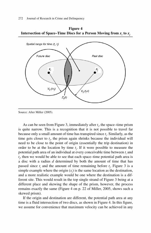
As can be seen from Figure 3, immediately after ti, the space–time prismis quite narrow. This is a recognition that it is not possible to travel farbecause only a small amount of time has transpired since ti. Similarly, as thetime gets closer to tj, the prism again shrinks because the individual willneed to be close to the point of origin (essentially the trip destination) inorder to be at the location by time tj. If it were possible to measure thepotential path area of an individual at every conceivable time between ti andtj, then we would be able to see that each space–time potential path area isa disc with a radius d determined by both the amount of time that haspassed since ti and the amount of time remaining before tj. Figure 3 is asimple example where the origin (xi) is the same location as the destination,and a more realistic example would be one where the destination is a dif-ferent site. This would result in the top single strand of Figure 3 being at adifferent place and skewing the shape of the prism, however, the processremains exactly the same (Figure 4 on p. 22 of Miller, 2005, shows such askewed prism).

If the origin and destination are different, the potential path area at anytime is a fluid intersection of two discs, as shown in Figure 4. In this figure,we assume for convenience that maximum velocity can be achieved in any


Figure 4Intersection of Space–Time Discs for a Person Moving from xi to xj

Source: After Miller (2005).

direction, though it is recognized that the real urban mosaic offers a rangeof barriers that limit travel speed in different places. If we assume that theimage relates to a journey taken by an offender who leaves xi at time ti andhas to be at xj at time tj, then at an intervening time denoted by t (whereti < t < tj), it is possible to estimate the area that the offender could occupyif maximum velocity is known. This area is described as a disc with a radiusof vij(t − ti)—maximum distance travelable in the time available at best speed.Using Miller’s (2005) notation, this area is fi(t), the set of locations that canbe reached from xi by the elapsed time t – ti. This is shown as:

fi(t) = {x⎪⎪x − xi⎪⎪≤ (t − ti)vij} (1)

The set fi(t) is a closed, convex set referred to as the future disc andshows the possible locations available in the future moment t from xi. Inthree-dimensional space, the shape is dictated by physical geography suchas hills, valleys, and buildings, but the point is most easily illustrated intwo-dimensional space. A two-dimensional approach is also the mostapplicable to crime researchers using a GIS to model offender behavior.

Similarly, if it is known when the offender has to be at xj, then the tem-poral constraint imposed by this commitment limits the range of places thatthe offender can occupy. This range is shown by a disc with a radius ofvij(tj – t)—maximum distance travelable in the time remaining at best speed.This range of locations that can reach xj in the remaining time budget oftj – t is pj(t), also known as the past disc, where:

pj(t) = {x⎪⎪xj − x⎪⎪≤ (tj − t)vij} (2)

The intersection of these discs (the area of Figure 4 denoted by the dark-est shading) shows the spatial range of the offender at time t. Given equa-tions (1) and (2), this disc intersection area is as follows:

Zij(t) = fi(t) ∩ pj(t) (3)

As time progresses, the area of the disc on the left will grow and the discon the right will shrink. The size of Zij(t) is dependent on the amount ofreserve time available to the individual undertaking the journey from xi

to xj. For example, if the journey time is 30 minutes, and the offender hasa temporal constraint (such as starting school or work) that requires themto be at the destination in 30 minutes’ time, then the two circles centeredrespectively on xi and xj will not overlap, but will just touch at their


circumferences. In other words, if the minimum travel time between xi andxj is t*

ij, where:

t*ij = ⎪⎪xj − xi⎪⎪vij (4)

then Zij(t) will be a single point if tj − ti = t*ij. If tj − ti ≤ t*

ij then it is notpossible to reach xj within the time budget available, and if tj − ti > t*

ij thenthere is reserve time available for other activities, including alternativeroute selection or offending. The two discs from Figure 4 centered on xi andxj are evaluated for one t as some time between ti and tj. If it were possibleto evaluate every t between the two time references then it could be possi-ble to construct a continuous series of discs and to evaluate Zij(t) for everymoment between ti and tj. The continued intersection of these discs fromti to tj describes an ellipse that is the aggregate spatial range of the offendergiven the spatio-temporal constraints of (xi, ti) and (xj, tj). This ellipse is thespatial range of the offender from time ti to tj and is shown in Figure 4 as alight grey ellipse. This general range of locations is described in equation 3.The ellipse is a two-dimensional shape with a foci of xi, xj, major axislength of (tj – ti)vij and minor axis of length [((tj − ti)vij)

2 − ⎪⎪xj − xi⎪⎪2]12–. As

Miller (2005) notes, this shape collapses to a circle when xi = xj.At present, we have not considered offending time. Most property

offending takes a certain amount of time and takes place at a stationarypoint, referred to in time geography as an activity time (aij). Although a sta-tionary activity, such as offending, is a temporal constraint (with a timebudget of the time required to commit the offense), in essence it also actsas a spatial constraint, limiting the full extent of d in Figure 3 by constrict-ing the prism at its widest point. This revision to the potential path area(PPA) is shown in Figure 5 where the constrained area (shaded in gray)denotes the smaller area to conduct the activity due to the amount of timeit takes to perform the activity (ai , aj). Note that although the journey startand end site is the same location (hypothetically an offender’s home orwork place) and is therefore shown as xi for both ends of the journey, it isequally possible that the offender moves to another location after theoffense (which would have been shown as xj at another location). For easeof comprehension, the graphic from Figure 3 is adjusted.

This additional constraint can be reflected in a revised estimation ofZij(t) if an activity is to be conducted, such that (from Miller 2005):

Zij(t) = fij(t) ∩ pj(t) ∩ gij (5)


where gij is the set of locations that can be reached from xi and still havetime to conduct the activity and reach xj by tj, such that:

gij = [((tj − ti − aij)vij)2 − ⎪⎪xj − xi⎪⎪

2]12–

(6)

The area Zij(t) is shown as dark gray shading in Figure 4. With this basicnotation in place, this article proceeds to place these concepts of space–timegeography into a criminological context by examining offender spatialbehavior.

Temporal Constraints and Criminal Behavior

From a criminological perspective, if a substantial proportion of offendercriminal behavior is largely driven by response to an opportunity encountered


Figure 5The Potential Path Area (PPA) from Figure 3is Now Constrained by the Need to Conduct

an Activity (a) for a Set Period of Time

during a non-crime-related journey, then the temporal constraints of nodeswill define offender exposure to criminal opportunities across space. Inessence, it will be the noncriminal activity that is foremost in defining thespatial arrangement of criminal opportunities for each offender. All of theconstraints that apply to any noncriminal activity will transfer to an offend-ing behavior pattern. For example, we can begin by thinking about noncrim-inal behaviors such as going to an airport to catch a flight or going to school.Most people do not travel to an airport days prior to a flight as there is littlevalue in waiting days before a departure. Most people therefore arrive at anairport from one to three hours before they are due to leave, anticipating theamount of time necessary to travel to the airport, check-in, and reach thedeparture gate, as well as building in a little extra time to allow for possibledelays in either getting to the airport or delays at the airport. We can think ofthe time budget allocated to these instances comprising of both a journeytime, being the time required to actually get to the airport, and a reserve timebeing the time left over to allow for unexpected problems. The reserve timecan easily be swallowed up by an accident on the way to the airport, or a longqueue at check-in. The temporal constraint is therefore defined as the time ofthe flight (tj) and the location of the airport (xj) relative to the starting point ofthe traveler (xi). These three parameters are used by people to determine whattime they should leave the starting point (ti). Greater reserve time allows foreither more time to loiter en route to or at the airport, or the option to takealternative routes. Reserve time not dedicated to travel therefore defines thepossibilities to use varying routes away from the predetermined (usually ashortest distance) route or to conduct other activities.

Similarly, consider a youth traveling from home to school. Most youngpeople aim to walk to school to arrive close to starting time. In other words, ifa youth has to be at school by 9 a.m., and the shortest journey time is 33 min-utes, then the student must leave home by 8:27 a.m. to avoid getting into trou-ble. If the student leaves home at 8:20 a.m., then there are only seven minutesavailable in the reserve time budget for route variation or other activities.

To demonstrate this in a two-dimensional format, consider Figure 6. Theintersection area Zij(t) for a 33-minute journey (with 40 available minutes)can be mapped for every minute for a journey from the example youth’shome to the destination (school). Using a GIS, it is possible to combine theindividual space–time discs (from Figure 4) that individually represent Zij(t)for each minute (equation 3) and in doing so show the ellipse that repre-sents the spatial range for time (ti, tj). If the individual Zij(t) discs are com-bined and their degree of overlap totaled, we can calculate the risk time forspecific locations on the offender’s available routes.


Figure 6 shows that locations on the immediate path of the offender areat potential risk for the greatest length of time. In other words, the youthcan loiter in these areas for the longest amount of time before having tocontinue the journey to the destination. The risk time rapidly reduces forlocations that are not located along the most direct path. The spatial rangeellipses for different reserve time budgets can be visualized by interpolat-ing from minute to minute. Of course, this example assumes that offendingtakes little or no time, but an adjustment can be made for this, as follows.

If the youth in this example has a propensity to graffiti, and if our exampleyouth’s tag requires five minutes to create, then the amount of reserve timeavailable to select a tag site is only two minutes. The five minutes requiredto create the tag suggests a stationary activity time (aij), which as explained


Figure 6Areas of Potential Crime Risk, Zij(t), Measured in Minutes,

for an Offender Traveling from Home to a Destination,with Seven Minutes Reserve Time, Assuming thatAny Offense Takes Little or No Time to Commit

Note: The street pattern is artificial and provided for context.

above, acts as a spatial constraint, revising the set of locations that can bereached from xi while still having time to reach xj by tj (see equation 6).

For our example youth intent on an act of graffiti, this temporal con-straint of actually conducting the activity (aij) leaves little time to exploremuch beyond the shortest path to school without running a risk of being lateand getting into trouble. The temporal constraint of the school starting timeacts as an inhibitor to straying far from the path between home and theschool. Greater exploration increases the chance of being late, assumingthat being late is something that the youth wishes to avoid and that latenesshas some sanction applied by the school. This is shown in Figure 7 wherethe Zij(t) discs have been recalculated to include a five minute offense time.In this way, each discs represents the revised spatial range of Zij(t) fromequation 5 (revised from equation 3).

Of course, the problem can be resolved by leaving home earlier, say at8 a.m.; however, if we concur that crime opportunities often arise as a resultof noncrime journeys (as stressed earlier) and if the trip to school originatesas a noncrime journey, then the youth would expect to arrive very early forschool (by 8:33 a.m.) and have to wait around half an hour for school tostart. Unobtrusive observations of 50 randomly selected elementary schoolchildren in Lincoln, Nebraska, found that after leaving school, 88 percentof the students walked directly to a residence, and 98 per cent chose a least-distance path from their school to their destination (Hill 1984). Arrivingcloser to the start time is the norm for school children as it is for adult lifeand the journey to work. In other words, although more crime opportunitiesbecome available if the journey is started earlier, why would an offenderbother if they did not originally anticipate that the trip would create crimeopportunities? If we accept the evidence produced earlier that many crimeevents are opportunity-based, then noncrime journeys would appear todominate the daily routine of offenders, and journeys close to the minimalpossible travel time budget would be the norm.

Time therefore acts as a constraint on offender movement, especiallyin relation to obligatory activities. The constraints placed on the offenderdirectly relate to the target risk. Returning to the example used in this section,as time creeps closer to 9 a.m. (school start time), the spatial location ofpotential targets for graffiti creeps closer to the school. The immediate vicinityof the youth’s home is not available for graffiti at 8:50 a.m. because theredoes not exist sufficient time to tag a site (five minutes) and then cover the33-minute journey to school. Property close to school is more at risk as 9 a.m.approaches because the impending commencement of the school day acts asa temporal constraint, forcing children into the vicinity of the school at this


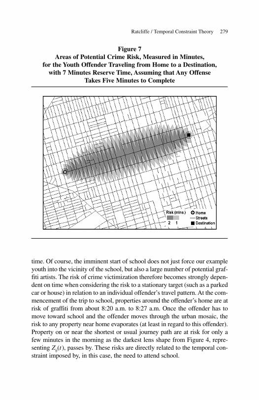
time. Of course, the imminent start of school does not just force our exampleyouth into the vicinity of the school, but also a large number of potential graf-fiti artists. The risk of crime victimization therefore becomes strongly depen-dent on time when considering the risk to a stationary target (such as a parkedcar or house) in relation to an individual offender’s travel pattern. At the com-mencement of the trip to school, properties around the offender’s home are atrisk of graffiti from about 8:20 a.m. to 8:27 a.m. Once the offender has tomove toward school and the offender moves through the urban mosaic, therisk to any property near home evaporates (at least in regard to this offender).Property on or near the shortest or usual journey path are at risk for only afew minutes in the morning as the darkest lens shape from Figure 4, repre-senting Zij(t), passes by. These risks are directly related to the temporal con-straint imposed by, in this case, the need to attend school.


Figure 7Areas of Potential Crime Risk, Measured in Minutes,

for the Youth Offender Traveling from Home to a Destination,with 7 Minutes Reserve Time, Assuming that Any Offense

Takes Five Minutes to Complete

This example demonstrates that if a potential offender’s temporalconstraints are known, then the potential risk to people and property can bemapped both spatially and temporally. Of course, it is also recognized thatthe model is most effective when the temporal constraint imposed by thetarget destination is an enforceable one that carries sanctions or a penaltyso as to realistically enforce the temporal constraint. This issue will bereturned to in the discussion.

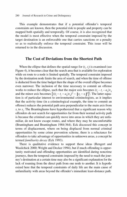
The Cost of Deviations from the Shortest Path

When the ellipse that defines the spatial range for (ti, tj) is examined (seeFigure 4), it becomes clear that the search area that is available for explorationwhile en route to a node is limited spatially. The temporal constraint imposedby the destination node limits the area of search, and when the time of offenseis deducted from the time budget then the shape of the overall ellipse becomeseven narrower. The inclusion of the time necessary to commit an offenseworks to reduce the ellipse, such that the major axis becomes (tj – ti – aij)vij

and the minor axis becomes [((tj − ti − aij)vij)2 − ⎪⎪xj − xi⎪⎪2]1

2–. The latter equa-

tion is of particular interest to environmental criminologists, as it impliesthat the activity time (in a criminological example, the time to commit anoffense) reduces the potential path area perpendicular to the main axis fromxi to xj. The Brantinghams have hypothesized that a significant reason whyoffenders do not search for opportunities far from their normal activity pathis because the criminal can quickly move into areas in which they are unfa-miliar, do not know escape routes, and where they may be uncomfortable(Brantingham and Brantingham 1984:364). Eck discussed this concept interms of displacement, where on being displaced from normal criminalopportunities by some crime prevention scheme, there is a reluctance foroffenders to take advantage of opportunities in unknown areas, a concept hetermed familiarity decay (Eck 1993).

There is qualitative evidence to support these ideas (Rengert andWasilchick 2000; Wright and Decker 1994), but if much offending is oppor-tunity motivated and offending opportunities are identified during noncrimejourneys, then the temporal constraints imposed by the need to reach the jour-ney’s destination at a certain time may also be a significant explanation for thelack of roaming from the direct path from one node to another. It is hypoth-esized here that the temporal constraints of daily life are the main cause ofunfamiliarity with areas beyond the offender’s immediate least-distance path.


Once an offender strays into unfamiliar territory, the average speed oftravel is likely to slow due to the necessity to negotiate unknown roads.A slower speed means that less territory is covered in the same time, and thearea of ground that can provide a criminal opportunity is reduced. Even if asteady speed can be maintained, any journey that deviates from the predom-inant direction will quickly erode available time for offending. For example,if an offender decides to turn perpendicular to the shortest distance path to anode, then the perpendicular journey eats into the time budget for the jour-ney. If the node is still to be reached by the required time, then the offenderwill quickly eat into all the available reserve time and will have to resumethe journey. Some deviations will still be in the general direction of the des-tination node, but as long as this is not along the shortest route, the relativedecrease in speed toward the destination will incur a time cost that can onlybe paid in part from the original time budget for the journey.

One Offender Searching from Home

Even when the offender is less opportunity-driven during an innocenttrip, deliberate crime risk is highly temporal for property. Consider an offenderwho has two spare hours to travel from home to seek out a criminal oppor-tunity such as a residential burglary, and then has to return home for somecommitment (for example, a youth may have been told by parents to behome by a certain time, or an individual may have a court-imposed curfew).Given a two-hour window of essentially reserve time, which is uncommit-ted to any obligatory activity, one might be tempted to think that all loca-tions within one hour’s walk of the home address are potentially at risk,however this is not the case. There are two significant temporal constraints.The first is the need to return to the domicile within two hours. The secondis to factor in the time required to commit an offense. For example, a burglarymight require 20 minutes, comprising 10 minutes to wait near the targetproperty to establish if the occupants are home, if they have an alarm andif there is a dog present; five minutes to effect an entry to the premises; andfive minutes to search the home and remove the property. Evidence frominterviews with burglars suggests that this estimate of 20 minutes lies some-where in the modal range (Rengert and Wasilchick 2000). Given a 20-minutetime span required to commit the offense, a crime site that is one hour fromthe offender’s home would allow no time to commit the offense. Althoughxi = xj, aij is 20 minutes and this reduces the available reserve time such thattj – ti = 100 minutes.


This means that if only one property is to be targeted (offense time20 minutes) then there is only a time budget of one hour and 40 minutes(100 minutes) available for searching for the target. Given the need to travelto and from the target, only properties within a 50-minute walk of theoffender’s home are effectively in range.

This picture becomes more complicated when the offender begins tosearch local streets closer to home first. The likelihood that a burglary willhappen at a home 50 minutes from the offender’s home address effectivelyevaporates as soon as a nonlinear search pattern is employed. Unless theoffender moves directly in one direction at best speed, the first route varia-tions will eat into time available to achieve the best range within the timeremaining before the offender has to be back home. For example, if theoffender searches close to home and has not left the vicinity of the homeaddress after 20 minutes, then the only locations that are at risk exist within40 minutes travel time from the offender home, bearing in mind that itrequires 20 minutes to commit the crime and the remaining 80 minutes hasto be divided into two to cover the time to get to and from the crime site.

Furthermore, the temporal constraint of having to return home at a cer-tain time will increase the risk closer to home more so than sites closer tothe extent of the 40-minute range. As range from home increases, thenumber of viable properties increases exponentially (Rengert, Piquero, andJones 1999) yet, if only one site is selected for burglary, the relative risk toeach site decreases. The temporal constraint of having to return homewithin two hours means that houses close to the offender’s home will be atrisk for most of the two-hour time period, whereas a location 45 minutesaway will only be theoretically at risk for a 10-minute block of time aroundthe middle of the two-hour time block. This is because it would take45 minutes to reach the area, 20 minutes to commit the crime, and 45 minutesto return home. This is a total of 110 minutes, leaving only 10 minutes leftof the two hours (120 minutes) to search for a viable target. If the offenderhas not identified a suitable target after 55 minutes, then there is not enoughtime to commit the crime and return. In this way, locations further from anoffender’s home tend to have a reduced time of risk to burglary.

This may help to provide a temporal rationale for the findings thatoffenses tend to cluster around an offender’s home (Rengert and Wasilchick2000). To this point, this clustering has been explained by both the leasteffort principle, which states people will not travel further than is necessaryto conduct an activity, and crime pattern theory, which hypothesizesthat locations close to home will be in an offender’s awareness space. Thetheory of temporal constraints proposed here supports this by suggesting


that constraints imposed by the need to be at nodes at certain times limitsoffending opportunities and concentrates risk close to home. Potential vic-timization will exist near nodes around the times that the temporal con-straint becomes effective, and for many offenders, their home is often aspatio-temporal constraint.

One Offender with Multiple Nodes

Given that most potential offenders will have more than one or twonodes in their daily routines, the spatial location of the nodes has a cumu-lative impact on the risk of crime on the paths between these nodes. Figure 8shows the spatial range for an individual located at the white cross, andtraveling to three different nodes (shown as black squares).1 If the individual’sbehavior is temporally constrained, the available routes to and from these


Figure 8Three Spatial Ranges Shown for an Offender Residing at

the White Cross, and Traveling to the Black Squares

Note: The risk to property is greatest in area A, where all three spatial ranges overlap. The riskalong each spatial range is also dependent on the temporal constraints of the destination.

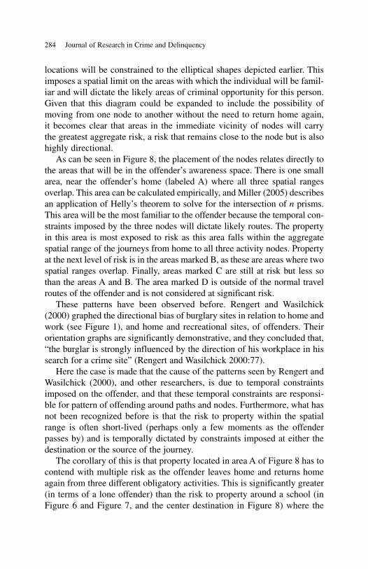
locations will be constrained to the elliptical shapes depicted earlier. Thisimposes a spatial limit on the areas with which the individual will be famil-iar and will dictate the likely areas of criminal opportunity for this person.Given that this diagram could be expanded to include the possibility ofmoving from one node to another without the need to return home again,it becomes clear that areas in the immediate vicinity of nodes will carrythe greatest aggregate risk, a risk that remains close to the node but is alsohighly directional.

As can be seen in Figure 8, the placement of the nodes relates directly tothe areas that will be in the offender’s awareness space. There is one smallarea, near the offender’s home (labeled A) where all three spatial rangesoverlap. This area can be calculated empirically, and Miller (2005) describesan application of Helly’s theorem to solve for the intersection of n prisms.This area will be the most familiar to the offender because the temporal con-straints imposed by the three nodes will dictate likely routes. The propertyin this area is most exposed to risk as this area falls within the aggregatespatial range of the journeys from home to all three activity nodes. Propertyat the next level of risk is in the areas marked B, as these are areas where twospatial ranges overlap. Finally, areas marked C are still at risk but less sothan the areas A and B. The area marked D is outside of the normal travelroutes of the offender and is not considered at significant risk.

These patterns have been observed before. Rengert and Wasilchick(2000) graphed the directional bias of burglary sites in relation to home andwork (see Figure 1), and home and recreational sites, of offenders. Theirorientation graphs are significantly demonstrative, and they concluded that,“the burglar is strongly influenced by the direction of his workplace in hissearch for a crime site” (Rengert and Wasilchick 2000:77).

Here the case is made that the cause of the patterns seen by Rengert andWasilchick (2000), and other researchers, is due to temporal constraintsimposed on the offender, and that these temporal constraints are responsi-ble for pattern of offending around paths and nodes. Furthermore, what hasnot been recognized before is that the risk to property within the spatialrange is often short-lived (perhaps only a few moments as the offenderpasses by) and is temporally dictated by constraints imposed at either thedestination or the source of the journey.

The corollary of this is that property located in area A of Figure 8 has tocontend with multiple risk as the offender leaves home and returns homeagain from three different obligatory activities. This is significantly greater(in terms of a lone offender) than the risk to property around a school (inFigure 6 and Figure 7, and the center destination in Figure 8) where the


temporal risk is greatest just before opening time and then just after finishingtime. Although this section has concentrated on the behavior of an individ-ual offender, it is clear that certain crime generators will impose temporalconstraints on victims and offenders alike, creating the conditions to fuelcrime at certain times. Home owners close to schools and to rowdy barsexperience this, as these locations bring people together all at one time, andoften disperse them at a set time. Crime in these areas is likely to be highlytemporally specific as a result.

Discussion

This article proposes that the spatio-temporal patterns of opportunity-basedcrime are highly dependent on the temporal constraints placed on offenders.These temporal constraints, such as work or going to school, influence thetravel patterns of noncrime journeys that are central in the identification ofopportunities for criminal activity. These travel patterns are affected in boththeir timing and route. It is hypothesized here that the temporal constraints ofdaily life are the main cause of unfamiliarity with areas beyond the offender’simmediate least-distance path. The corollary of this is that temporal con-straints, in conjunction with the locations of offender nodes, are a major deter-minant in spatio-temporal patterns of property crime.

Furthermore, this temporal constraint theory implies that the risk toproperty from an offender is often brief and dynamic lasting for only a fewminutes or even moments, but doing so at a fairly regular time each day.The opportunity to commit crime will also be affected by the temporalconstraints placed on victims, patterns of behavior to which offenders areknown to be sensitive (Rengert and Wasilchick 2000), and which have ameasurable impact on crime (Cohen and Felson 1979).

Society has long understood this relationship between temporal and spatialpatterns and the need for constraints. Prison remains one of the ultimate spatio-temporal constraints that can be imposed on a known offender, and truancyprograms and curfews are more limited attempts to restrict the spatio-temporalfreedom of potential offenders. Truancy is a recognized risk factor in delin-quency, though there is a current lack of rigorous testing of the crime-preventionbenefit of truancy programs (Sherman et al. 1998). From a temporal-constraintperspective, truancy prevention may be effective in reducing residential bur-glary. Given that residential burglary is a predominantly daytime crime, thetime of risk is generally during school hours. By requiring a school child toremain at school, this temporal constraint limits their movement during the


time of greatest residential burglary activity. For the majority of residentialburglars, the ideal opportunity is to break into an unoccupied home. Thisrequirement creates a constraint to wait until all of the household occupantshave gone to school or work, and provides an additional constraint to completethe crime before children come home from school or adults return from work.Once school has finished, then returning parents or the presence of schoolchildren in the home acts as a victim-induced constraint.

Late-night curfews, on the other hand, are less likely to act as a temporalconstraint on residential burglary, however they may act as a temporal con-straint on nonresidential burglary and crimes of violence or criminal dam-age. In some states and countries (e.g., New Zealand) it is common toimpose a court-ordered curfew as a bail condition and police are entitled toconduct bail checks to ensure that the offender is at home during the curfewhours. These are often dusk to dawn curfews, however, a greater under-standing of the temporal patterns of crime (such as residential burglary) mayimprove the facility of curfews by timing them to coincide with the times ofoffending of the individual in question. This would impose a temporal con-straint of being at their home address during the highest offending time.

Temporal constraints are most likely to function as an inhibitor to crime-search behavior when the purpose of the journey is primarily noncriminaland there is an obligatory activity awaiting the offender at the destinationnode; in other words, a journey related to a noncrime compulsory activity.When the temporal constraint at the destination is more fluid, or discre-tionary, then there exists the possibility of trading more time between thereserve and the journey time budgets. For example, if an offender agrees tomeet a friend in a bar for an evening, arrival time is usually flexible withinsocial limits. The temporal constraint of meeting friends is therefore ofmore limited value as a crime inhibitor. Of more value are activities such aswork which acts as a strong temporal constraint forcing an individual toremain at one location for a number of hours in each work day. Even whenan employee has a free lunch hour, the constraints of having to return towork within an hour severely hampers the spatial range away from theworkplace that can be targeted as well as limiting the available time foroffending and criminal opportunity search.

Although 88 percent of the elementary school children reported by Hill(1984) walked directly to a residence after school, it is more likely thatolder children and teenagers will have the time to vary their route and activ-ities after school. The temporal constraint of getting to school on time isless likely to be replaced by a similarly rigid restraint after school, thoughafter-school programs and sports activities could fulfill this role. It is also


recognized that a number of offenders are less likely to have attachmentsto, and be constrained by, social institutions that provide conventionalactivities. Their perception of time may also be more fluid than that of thelaw-abiding, though this could be changing at a societal level. It may be thatas traffic congestion increases in our urban centers, and some people areable to work from home more than before, it is becoming increasinglyacceptable to be late. If we increasingly accept workers and students arriv-ing late for fixed activities, this changes the patterns of temporal constraintfor offenders and victims. A further caveat should be noted here: it is likelythat offenders in possession of stolen properly and vulnerable to detectionby the police may travel at a faster speed homeward (or toward a criminalfence) than the outward journey.

It should be stressed that property owners should not lower their guardsimply because the time that an offender may pass by has concluded.Although there are times when the routine activities of offenders bringsthem within visual range of a home or parked vehicle, this does not neces-sarily mean that this is the time that a crime will occur. It should be remem-bered from the ethnographic research of Wright and Decker (1994) that evenwhen offenders deliberately seek a burglary opportunity, they go to homesthat they had identified through noncriminal journeys, or search in familiarareas. The potential for an offense may therefore be greatest when theoffender is not temporally constrained but has more free time, perhaps whennot going to work for example. Given that the majority of the offenders inter-viewed by Wright and Decker deliberately sought out criminal opportunities,property should be protected at all times. However, the situational crimeprevention key may be to make the house (as an example of a popular crim-inal target) appear particularly well-protected or occupied at the times whenthe offender is passing by on the noncrime journey. For example, althoughresidents near schools should always be crime-aware, they should be cog-nitive that many potential offenders are walking past their home just priorto school starting, and just after school is finishing. As a result, giving theappearance that the home is occupied and secure during these particulartimes may signal to offenders to seek out other opportunities away from thislocation when they return to the area for criminal activity later in the day.

Conclusion

It is recognized that this is not a universal theory that explains all offend-ing patterns. Temporal constraints are only as good as their ability to influence


potential offender behavior and the emphasis in this article on rigid temporalconstraints is a simplifying assumption, one that is deliberately applied to aidcomprehension of the concept. Recidivist offenders and career criminals willbe less influenced by constraints such as the start of the school bell. Minorinfractions, such as starting school or work a few minutes late, will providefor an increase in opportunity to commit crime, however, time-measurementtheory is able to include those calculations (where known) and to expand themodel of property risk accordingly. Time-measurement theory is also able toinclude an adjustment for the time required to escape from a crime scene, afeature that is a consideration in some offenses.

The empirical notation from Miller (2005) provides a roadmap toresearchers wishing to more formally express the importance of time as aconstraint on offender behavior. This greater quantification of what hasbeen a recognized yet fuzzy parameter has implications for both researchand policy. Researchers, especially those interested in agent-based model-ing, may benefit from a more formal mechanism to express the behavior ofoffenders and victims across the urban mosaic. Practitioners wishing tobetter incorporate time into their offender control strategies may find valuein this, and hopefully subsequent, work to formalize the spatio-temporalbehavior of offenders, and recognize the value of introducing temporal con-straints within the community.

The next stage in this work is to re-examine offender spatial behaviorpatterns with a greater emphasis on the temporal constraints that are part oftheir lives and which frame their offending opportunities and to constructexplanatory models using time measurement theory.

Note

1. For convenience of illustration, the varying risk within the spatial range is not shown,nor is the distinct possibility of moving from one node to another without having to returnhome again.

References

Anderson, D., S. Chenery, and K. Pease. 1995. “Biting Back: Tackling Repeat Burglary andCar Crime.” Police Research Group: Crime Detection and Prevention Series Paper 58:1-57.

Barr, Robert and Ken Pease. 1990. “Crime Placement, Displacement, and Deflection.”Pp. 277-318 in Crime and Justice: An Annual Review of Research, vol. 12, edited by M. Tonryand N. Morris. Chicago: University of Chicago Press.


Bowers, Kate J., Alex Hirschfield, and Shane D. Johnson. 1998. “Victimization Revisited.” BritishJournal of Criminology 38:429-52.

Brantingham, Patricia and Paul Brantingham. 1981. “Introduction: The Dimensions of Crime.”Pp. 7-26 in Environmental Criminology, edited by P. J. Brantingham and P. L. Brantingham.London: Waveland Press.

______. 1984. Patterns in Crime. New York: Macmillan.______. 1993. “Nodes, paths and edges: Considerations on the Complexity of Crime and the

Physical Environment.” Environmental Psychology 13:3-28.______. 1995. “Criminality of Place: Crime Generators and Crime Attractors.” European

Journal of Criminal Policy and Research 3:5-26.Burquest, R., G. Farrell, and K. Pease. 1992. “Lessons from Schools.” Policing 8:148-55.Chainey, Spencer and Jerry H. Ratcliffe. 2005. GIS and Crime Mapping. London: Wiley.Clarke, R.V. and D. Weisburd. 1994. “Diffusion of Crime Control Benefits.” Pp. 165-83 in Crime

Prevention Studies, vol. 2, Crime Prevention Studies, edited by R. V. Clarke. Monsey, NY:Criminal Justice Press.

Clarke, Ronald V. and Derek B. Cornish. 1985. “Modeling Offenders’ Decisions: A Frameworkfor Research and Policy.” Pp. 147-85 in Crime and Justice: An Annual Review of Research,vol. 6, edited by M. Tonry and N. Morris. Chicago: University of Chicago Press.

Clarke, Ronald V. and Marcus Felson. 1993. “Introduction: Criminology, Routine Activity, andRational Choice.” Pp. 259-94 in Routine Activity and Rational Choice, vol. 5, Advances inCriminological Theory, edited by R. V. Clarke and M. Felson. New Brunswick: Transaction.

Cohen, Lawrence E. and Marcus Felson. 1979. “Social Change and Crime Rate Trends:A Routine Activity Approach.” American Sociological Review 44:588-608.

Cornish, Derek and Ron Clarke. 1986. The Reasoning Criminal: Rational Choice Perspectiveson Offending. New York: Springer-Verlag.

Costello, Andrew and Paul Wiles. 2001. “GIS and the Journey to Crime.” Pp. 27-60 inMapping and Analysing Crime Data edited by K. Bowers and A. Hirschfield. London:Taylor and Francis.

Cromwell, Paul F., James N. Olson, and D’Aunn Wester Avary. 1991. Breaking and Entering:An Ethnographic Analysis of Burglary, vol. 8. Newbury Park, CA: Sage.

______. 1999. “Decision Strategies of Residential Burglars.” Pp. 50-6 in In Their Own Words:Criminals on Crime, edited by P. Cromwell. Los Angeles: Roxbury.

Eck, J. 1993. “The Threat of Crime Displacement.” Criminal Justice Abstracts 25:527-46.Eck, J. E. and W. Spelman. 1987. “Problem Solving: Problem-Oriented Policing in Newport

News.” Police Executive Research Forum, Washington DC.Farrell, G. and K. Pease. 1994. “Crime Seasonality—Domestic Disputes and Residential

Burglary in Merseyside 1988-90.” British Journal of Criminology 34:487-98.Felson, Marcus. 1995. “Those Who Discourage Crime.” Pp. 53-66 in Crime and place, vol. 4,

edited by D. Weisburd and J. E. Eck. Monsey, NY: Criminal Justice Press.______. 1998. Crime and everyday life: Impact and implications for society. Thousand Oaks,

CA: Pine Forge Press. Felson, Marcus and Ronald V. Clarke. 1998. “Opportunity Makes the Thief: Practical Theory

for Crime Prevention.” Police Research Group: Police Research Series Paper 98:36.Goldstein, Herman. 1990. Problem-Oriented Policing. New York: McGraw-Hill.Green, Lorraine. 1995. “Cleaning Up Drug Hot Spots in Oakland, California: The Displacement

and Diffusion Effects.” Justice Quarterly 12:737-54.Groff, Elizabeth R and Nancy LaVigne. 2001. “Mapping an Opportunity Surface of Residential

Burglary.” Journal of Research in Crime and Delinquency 38:257-78.


Guerry, Andre-Michel. 1833. Essai sur la Statistique Morale de la France: Precede d’unRapport a l’Academie de Sciences. Paris: Chez Crochard.

Hägerstrand, Torsten. 1970. “What About People in Regional Science?” Papers in RegionalScience 24:7-21.

Hakim, Simon, George F. Rengert, and Yochanan Shachmurove. 2001. “Target Search ofBurglars: A Revised Economic Model.” Papers in Regional Science 80:121-37.

Harries, Keith. 1999. Mapping Crime: Principles and Practice. Washington, DC: U.S.Department of Justice.

Hesseling, R. 1994. Displacement: A Review of the Empirical Literature, vol. 3, edited byR. V. Clarke. Monsey, NY: Criminal Justice Press.

Hill, M. R. 1984. “Walking Straight Home from School: Pedestrian Route Choice by YoungChildren.” Transportation Research Record 959:51-5.

Jeffery, C. Ray and Diane L. Zahm. 1993. “Crime Prevention through Environmental Design,Opportunity Theory, and Rational Choice Models.” Pp. 323-50 in Routine Activity andRational Choice, vol. 5, Advances in Criminological Theory, edited by R. V. Clarke andM. Felson. New Brunswick: Transaction.

Leigh, Adrian, Tim Read, and Nick Tilley. 1998. “Brit Pop II: Problem-Orientated Policing inPractice.” Police Research Group: Police Research Series Paper 93:60.

Maguire, Mike. 1982. Burglary in a Dwelling. Liverpool, UK: Heinemann.Martin, David. 2002. “Spatial Patterns in Residential Burglary: Assessing the Effect of Neighbor-

hood Social Capital.” Journal of Contemporary Criminal Justice 18:132-46.Miller, Harvey J. 2005. “A Measurement Theory for Time Geography.” Geographical Analysis

37:17-45.Ratcliffe, Jerry H. 2000. “Aoristic Analysis: The Spatial Interpretation of Unspecific Temporal

Events.” International Journal of Geographical Information Science 14:669-79.______. 2001. “Policing Urban Burglary.” Trends and Issues in Crime and Criminal Justice

No. 213.______. 2002. “Aoristic Signatures and the Temporal Analysis of High Volume Crime

Patterns.” Journal of Quantitative Criminology 18:23-43.______. 2003. “ Suburb Boundaries and Residential Burglars.” Trends and Issues in Crime and

Criminal Justice No. 246.Ratcliffe, Jerry H. and Michael J. McCullagh. 1999. “Burglary, Victimisation, and Social

Deprivation.” Crime Prevention and Community Safety: An international journal 1:37-46.Rengert, George F. 1992. “The Journey to Crime: Conceptual Foundations and Policy

Implications.” Pp. 109-17 in Crime, Policing and Place: Essays in EnvironmentalCriminology, edited by D. J. Evans, N. R. Fyfe, and D. T. Herbert. London: Routledge.

Rengert, George F., Alex R. Piquero, and Peter R. Jones. 1999. “Distance Decay Reexamined.”Criminology 37:427-45.

Rengert, George F. and J. Wasilchick. 1985. Suburban Burglary: A Time and Place forEverything. Springfield, IL: C.C. Thomas.

______. 2000. Suburban Burglary: A Tale of Two Suburbs. Springfield, IL: C.C. Thomas.Robinson, Matthew B. 1999. “Lifestyles, Routine Activities, and Residential Burglary

Victimization.” Journal of Crime and Justice 22:27-56.Rossmo, D. Kim. 2000. Geographic Profiling. Boca Raton, FL: CRC Press.Scott, Michael S. 2000. Problem-Oriented Policing: Reflections on the First 20 Years.

Washington, DC: COPS Office.Sherman, Lawrence W., Denise Gottfredson, Doris MacKenzie, John Eck, Peter Reuter, and

Shawn Bushway. 1998. Preventing Crime: What Works, What Doesn’t, What’s Promising.Washington, DC: National Institute of Justice.


Taylor, R. B. 2002. “Crime Prevention through Environmental Design: Yes, No, Maybe,Unknowable, and All of the Above.” Pp. 413-26 in Handbook of Environmental Psychology,edited by R. Bechtel and A. Churchman. New York: John Wiley.

Tilley, Nick. 1993. “Understanding Car Parks, Crime and CCTV: Evaluation Lessons fromSafer Cities.” Police Research Group: Crime Prevention Unit Series Paper 42:33.

Tilley, Nick and Janice Webb. 1994. “Burglary Reduction: Findings from Safer Cities Schemes.”Police Research Group: Crime Prevention Unit Paper No 51:60.

Townsley, Michael, Ross Homel, and Janet Chaseling. 2000. “Repeat Burglary Victimisation:Spatial and Temporal Patterns.” Australian and New Zealand Journal of Criminology 33:37-63.

Weisburd, D and L Green. 1995. “Measuring Immediate Spatial Displacement: MethodologicalIssues and Problems.” Pp. 349-61 in Crime and Place, vol. 4, Crime Prevention Studies,edited by J. E. Eck and D. Weisburd. Monsey, NY: Criminal Justice Press.

Wiles, Paul and Andrew Costello. 2000. “The ‘Road to Nowhere’: The Evidence for TravellingCriminals.” London: Research, Development and Statistics Directorate (Home Office).

Wright, R. and S. Decker. 1994. Burglars on the Job. Boston: Northeastern University Press.Wu, Yi-Hwa and Harvey J. Miller. 2001. “Computational Tools for Measuring Space-Time

Accessibility within Dynamic Flow Transportation Networks. “Journal of Transportationand Statistics 4:1-14.

Jerry H. Ratcliffe is an associate professor of criminal justice at Temple University. He is aformer British police officer whose articles and books focus on environmental criminology,crime mapping, and police intelligence and analysis. He has a BSc and PhD from the Universityof Nottingham.


Journal of Research in Crime and Delinquency Volume 43 ... · Theory to Explain Opportunity-Based...

Documents

Transcript of Journal of Research in Crime and Delinquency Volume 43 ... · Theory to Explain Opportunity-Based...