Journal of Mathematical Economics 44 (2008) 1398–1412

Contents lists available at ScienceDirect

Journal of Mathematical Economics

journa l homepage: www.e lsev ier .com/ locate / jmateco

Stable processes of exchange

Stanley Reitera,∗, Spiro Maroulisb

a Economics, Mathematics, and Managerial Economics and Decision Sciences, College of Arts and Sciences and Kellogg School of Management, NorthwesternUniversity, United Statesb Department of Managerial Economics and Decision Sciences, Kellogg School of Management, Northwestern University, United States

a r t i c l e i n f o

Article history:Received 11 December 2007Received in revised form 15 July 2008Accepted 15 July 2008Available online 5 August 2008

Keywords:General equilibriumAgent-based modeling

a b s t r a c t

In this paper we address a long standing gap in economic theory—the gap between claimsfor the dynamic efficiency of trading in markets, and the findings of formal economic theory,which justify those claims only under restrictive assumptions. We use agent-based methodsto study the dynamics of exchange with trading agents who are characterized by severaldifferent preference relations. We see that outcomes converge with high probability toPareto optima in the cases studied, including the well-known example due to Scarf.

© 2008 Elsevier B.V. All rights reserved.

1. Introduction

This paper presents a dynamic process of exchange – trading – and explores its properties in several different economicsettings. Trading remains an interesting subject in economics, even after some 200 years of analysis and discussion, becausethe textbook paradigm according to which trading takes place in markets, market prices adjust in response to excess demandand converge to a static equilibrium is not supported by formal theory when there are three or more commodities, anddemand functions are general.

Introductory economics textbooks present trade as taking place in markets in which each individuals’ behavior is rep-resented by a demand or supply function whose argument is the vector of market prices. This is typically presented inelementary textbooks for the case of one or two commodities. These individual functions are aggregated into market demandand supply functions, or market excess demand functions, which define a system of equations in prices whose solution is theequilibrium market price vector—the market-clearing prices. The process by which prices adjust and supposedly convergeto an equilibrium price vector is discussed, and the conditions on market excess demand functions that assure convergenceof prices to the market-clearing prices are also discussed; this discussion is valid in the case of one or two commodities. Thisdiscussion of exchange is used in introductory texts not only because the modeling and analysis can be presented graphically,but perhaps also because the concepts of markets and of market prices appear to be indispensable to understanding tradeand exchange. There was also a hope, if not a conviction, that our understanding of exchange would remain the same inan economy with three or more commodities—that prices would adjust dynamically to excess demand and converge to thestatic equilibrium prices in all markets.

The appeal of this story to economists is very strong. Instead of having to deal with the individual behaviors of many agentsin a world of many commodities, the behavior of agents is described by their excess demand functions, and aggregated acrossagents into market excess demand functions. These form a system of equations whose solution is the general equilibrium—thesimultaneous equilibrium of all markets.

∗ Corresponding author.E-mail address: s-reiter@kellogg.northwestern.edu (S. Reiter).

0304-4068/$ – see front matter © 2008 Elsevier B.V. All rights reserved.doi:10.1016/j.jmateco.2008.07.012

S. Reiter, S. Maroulis / Journal of Mathematical Economics 44 (2008) 1398–1412 1399

It took about 150 years, and much intellectual effort, to go from Adam Smith’s insights into the efficacy of markets to arigorous formulation of the general equilibrium of an economy and to an understanding of the conditions under which ageneral equilibrium exists and has its now familiar optimality properties. The general equilibrium results confirm that theessential insight expressed in the story of static equilibrium of a two-commodity textbook economy also holds under certainnow well-established conditions for any finite number of commodities and economic agents.1

The next step was to show that the system of markets and prices will, starting from an arbitrary disequilibrium state findan equilibrium price vector. This would show that the textbook story for the case of two commodities – a story of convergencefrom non-equilibrium prices to an equilibrium price vector – is valid for the full class of economic environments in whichgeneral equilibrium exists, and has the optimality properties established for it in the static model.

The approach of aggregating individual behaviors as represented by individual excess demand functions into marketexcess demand functions led to a dynamics that looks very much like Newtonian dynamics—a system of differential equationsin prices whose dynamic adjustment depends on the excess demands for all commodities.2 Inconveniently for economictheory, it has been definitively shown that this dynamic system converges to competitive equilibria only in a restricted classof economic environments, a class too restricted to make this result satisfactory. For instance, Scarf’s example (1960), whichshows that any continuous function of prices that is homogeneous of degree zero, satisfies Walras’ Law, and a condition called‘desirability,’ can be an excess demand function in an exchange economy—illustrates that the class of economic environmentfor which Smith’s insight is valid is too limited to justify general claims of efficiency of markets.3 Indeed, it is now well-established that the classical approach does not find a static general equilibrium in the full class of economies in whichgeneral equilibrium exists and has the optimality properties established for it by the now classical welfare theorems ofgeneral equilibrium theory.

Frank Hahn’s essay “Stability” (1982) reviews the literature on stability of exchange up to about 1978. Most, but notall, of that literature discusses exchange in markets where agents are characterized by excess demand functions. Otherapproaches include processes inspired by Edgeworth’s recontracting process, and still others are processes based on dis-tributed algorithms for computing equilibria. Most of the mathematical formulations of the problem follow Samuelson(1941, 1942, 1947) in using differential (or difference) equations to model the simultaneous adjustment of commodityprices across markets. Perhaps influenced by a desire to stay within the mathematical structure of differential equations,Smale proposed a dynamic model based on Newton’s method for solving non-linear equations. Smale’s price adjustmentprocess (1976a,b) converges to an equilibrium price vector provided that it starts from a price vector near the boundaryof the price simplex—the domain of relative prices. This is awkward, and calls into question the economic interpreta-tion of the dynamics. Moreover, analysis by Saari and Simon (1978) shows that Smale’s process must use essentially allthe entries in the Jacobian matrix associated with the differential equations. This imposes an impractically large burdenof information—one that would make the dynamic process infeasible for all but tiny economies. Subsequently, Jordan(1987) showed that for a broad class of adjustment mechanisms, including excess demand dynamics, any continuous timeadjustment process that is locally stable at a Walrasian equilibrium must use messages large enough for each trader tocommunicate both his excess demand and the derivatives of his excess demand at the current prices. Jordan’s conclusion is:“the well-known informational efficiency of the competitive allocation mechanism is limited to the static model” (1987, p.194).

The situation outlined in the preceding paragraphs reveals a gap between claims for the dynamic efficiency of marketsfound in introductory textbooks – and in some popular writings – and the findings of formal theory. This gap presentseconomists with a challenge. Responses to this challenge have generated a large literature aimed at providing a foundationin theory for claims about how economic institutions could lead to ‘optimal’ or ‘efficient’ economic exchange, and have ledto a search for alternatives to excess demand price dynamics.

One line of response to this challenge has its roots in computer science. Developments in distributed computation haveinspired research in which computational algorithms—including distributed computational processes find – compute –market equilibria, or optima. There are many ingenious algorithms in this literature—too many to review here. But wemention one approach that seems to us closest to economic processes, and also illustrates a serious difficulty with dynamicsbased on computational algorithms.

Scarf (1960) and Kuhn (1968) present two different processes for computing an equilibrium price vector. The two processesare dual to one another. Joosten and Talman (1993) presented a process that combines Scarf’s algorithm with Kuhn’s, creatingthree algorithms that share a common feature; the shared feature is that the order in which prices are adjusted is part of theprocess.4 We quote: “In the process, the price of the commodity having the highest excess demand is initially increased, andsimultaneously the price of the commodity having the highest excess supply . . . is decreased. The prices of other commoditiesare initially not changed.”

1 The literature on general equilibrium theory is very large. Arrow (1951) contains the pioneering analysis. Debreu (1959) is a widely used source for thisliterature.

2 Samuelson (1941) presented an important mathematical formulation of these dynamics in economic theory. Samuelson refers to Walras’ idea oftâtonnement (Walras, 1954), an idea that is at the foundation of many attempts to model the dynamics of exchange.

3 See Scarf (1960) together with the papers Sonnenschein (1972, 1973), Shafer and Sonnenschein (1982) and references cited there. The papers Arrowand Hurwicz (1958, 1960) show restricted classes of cases for which the textbook claims are valid.

4 They also cite a number of other papers that take similar approaches.

1400 S. Reiter, S. Maroulis / Journal of Mathematical Economics 44 (2008) 1398–1412

One difficulty with processes of this kind is that the selection of the prices to be adjusted initially, and those not to bechanged initially, is not an activity that can be expected to be part of a ‘natural’ economy, especially a large one. Who is to figureout which commodity is in highest (or lowest) excess demand, and then adjust the price? As useful as distributed algorithmsmight be for computing, their application to dynamics of exchange is problematic. Adam Smith’s famous observation is, toparaphrase, that ‘the market’ functions so that independent actions of each of a multitude of people, each motivated by hisown interest, leads ‘as if by an invisible hand’ to an efficient economic outcome. This suggests that a distributed algorithmthat computes equilibria would have to be executed spontaneously by individual agents who are not taught their steps inthe algorithm. It seems that the analogy between free exchange among agents and distributed computation in a computernetwork works only one way—for our purposes, the wrong way.

Another line of response (also discussed by Hahn) uses approaches more closely related to Edgeworth’s exchange modelthan to excess demand models. This latter group includes a paper that presents a stochastic process of bids and exchanges—theB-process studied by Hurwicz et al. (1975a,b), briefly HRR.5 They show that the B-process converges to Pareto optima in aclass of environments that includes ones in which the competitive mechanism has (static) equilibria, and also ones in whichit is not guaranteed that static competitive equilibria exist, or exist and are Pareto optimal.6 For instance, in environmentswith indivisibilities or other non-convexities competitive equilibria might fail to exist, or, if they do exist, might not be Paretooptimal.7 The focus in HRR is on the analysis of the stochastic process that models the behavior of economic agents, and onthe consequences of their interactions, and compares the outcomes to those of standard economic theory. At each step ofthe B-process an array of proposed trades – bids– is determined to be consistent or inconsistent —adds up to the zero vector,or not. The HRR paper leaves open the details of the process by which such a determination is accomplished.8

There is also a substantial literature reporting laboratory experiments in trading. These have so far been necessarily smallscale, with a limited number of agents and a limited number of commodities. In many experiments that involve trading,demand or supply functions are induced in the experimental subjects by the experimenter in order to simulate a textbookmarket in which prices are adjusted in response to behavior that results from the induced demand and supply functions.Experiments tend to show that the behavior of experimental subjects is roughly consistent with what economic theoryassumes. It is not clear how much of the behavior observed in small scale experimental settings survives in a large economy,especially in sectors of the economy in which trading is not formally structured by organized markets. Vernon Smith andCharles Plott have pioneered this approach to studying trading.

To summarize, the now classical results of static general equilibrium theory – the classical welfare theorems – do nothave the force they would have if general equilibrium were shown to be dynamically stable. A theorem to that effect wouldbe the foundation for a claim that an economy organized by competitive markets would find competitive equilibria, to whichthe classical welfare theorems would apply, and so constitute a formal verification of Adam Smith’s insight. This state ofaffairs set in motion a search for an alternative to the classical excess demand dynamics of price adjustment. That search hasgenerated a large literature in which a variety of approaches is represented. The search continues.

This paper is a contribution to that literature. More specifically, we use the modern computational approach of agent-basedmodeling in an attempt to overcome the longstanding problems with the classical (Newtonian) dynamics. To understand thisapproach it is suggestive to consider dynamic behavior of societies of non-human living creatures—for example, honey bees.Honey bees live in fairly complex societies that exhibit specialization in their activities. Bees perform specialized activitiesby which the processes needed to maintain the society of the hive are carried out. Of course, a society of bees is muchsimpler than a human society, but both require internal communications to coordinate the actions by which the economyfunctions and is able to maintain the society. Other animal and insect societies exhibit similar problems of coordination, andassociated needs for communication. Generally, such processes of social coordination of activity are not well representedby differential equations models of aggregate phenomena; agent-based models appear to do better in some cases (Millerand Page, 2007). Moreover, in comparison to other computational approaches that have been used to study the dynamics ofexchange, agent-based models provide for a more plausible and straightforward interpretation of the behavior of economicagents.

Building on the ideas of HRR’s B-process, the economic agents are “boundedly rational”; we use stochastic elements inmodeling behavior; the processes of trading are not aggregated—the trading behavior and transactions of individual agentsare followed separately; and there are no prices. To explore and understand the dynamic performance of our decentralized andstochastic trading processes, we develop and experiment with computational, agent-based models.9 We demonstrate that adecentralized, agent-based process can find efficient outcomes in economies with multiple agents and three-commodities,including the cases like the Scarf example that have historically posed problems for economic theory. We do not attempt toprovide formal theorems and proofs of our ideas. Instead, the focus is on the dynamic process and its long-run tendency,

5 The B-process is based on a process presented by Reiter at a conference held at Purdue University in 1959 (Reiter, 1959), and also appeared in Reiter(1981).

6 The B-process is defined for both discrete and Euclidean commodity spaces. It accommodates production as well as exchange. The HRR papers do notanalyze the speed of convergence. Subsequently, Bala (1988) investigated the speed of convergence of the B-process, and, to summarize very briefly, foundthat it converges rather fast in the examples studied.

7 Stimulated by the B-process, Matsui (1981) proposed a stochastic adjustment process for non-convex and indecomposable environments.8 Hahn interpreted it as requiring a central agent who functions like the Walrasian auctioneer. This is not so, as the present paper shows.9 The models are developed using the NetLogo Programmable Modeling Environment (Wilensky, 1999).

S. Reiter, S. Maroulis / Journal of Mathematical Economics 44 (2008) 1398–1412 1401

with the larger goal of this work being to provide an example of how an agent-based framework can be used to tackle thestill unsolved problem of the stability of equilibria.

We turn now to a description of our model of trading.

2. A dynamic model of exchange

2.1. Overview

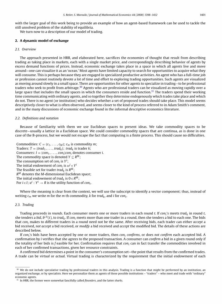
The approach presented in HRR, and elaborated here, sacrifices the economies of thought that result from describingtrading as taking place in markets, each with a single market price, and correspondingly describing behavior of agents byexcess demand functions of prices. Instead, economic exchange takes place in a space in which all agents live and movearound—one can visualize it as an ‘ocean.’ Most agents have limited capacity to search for opportunities to acquire what theywill consume. This is perhaps because they are engaged in specialized productive activities. An agent who has a full-time jobor profession cannot routinely devote a lot of time and effort to exploring trading opportunities. Such agents are visualizedas moving around slowly in a small space. There are opportunities for other agents to specialize in trading—to be professionaltraders who seek to profit from arbitrage.10 Agents who are professional traders can be visualized as moving rapidly over alarge space that includes the small spaces in which the consumers reside and function.11 The traders spend their workingtime communicating with ordinary agents, and so together they determine endogenously which trades take place and whichdo not. There is no agent (or institution) who decides whether a set of proposed trades should take place. This model seemsdescriptively closer to what is often observed, and seems closer to the kind of process referred to in Adam Smith’s comment,and in the many discussions of economic exchange found in the informal descriptive economics literature.

2.2. Definitions and notation

Because of familiarity with them we use Euclidean spaces to present ideas. We take commodity spaces to bediscrete—usually a lattice in a Euclidean space. We could consider commodity spaces that are continua, as is done in onecase of the B-process, but we would not escape the fact that computing is a finite process. This should cause no difficulties.

Commodities: C = {c1, . . . , cM}; cm is commodity m;Traders: T = {trad1, . . . , tradk}; tradk is trader k;Consumers: I = {con1, . . . , coni}coni denotes consumer i.The commodity space is denoted Y ⊆ RM;The consumption set of coni is Yi;The initial endowment of coni is ωi ∈ Yi

The feasible set for trader tradk is RM;RM denotes the M-dimensional Euclidean space;The initial endowment of tradk is 0 ∈ RM;For i ∈ I; ui : Yi → R is the utility function of coni.

Where the meaning is clear from the context, we will use the subscript to identify a vector component; thus, instead ofwriting cm we write m for the m th commodity, k for tradk, and i for coni.

2.3. Trading

Trading proceeds in rounds. Each consumer meets one or more traders in each round t. If coni’s meets tradk in round t,she tenders a bid, bi,k(t), to tradk. If coni meets more than one trader in a round, then she tenders a bid to each one. The bidsthat coni makes to different traders in a round need not be the same. After receiving bids, each trader can either accept abid received, not accept a bid received, or modify a bid received and accept the modified bid. The details of these actions aredescribed below.

If coni’s bids have been accepted by one or more traders, then coni confirms, or does not confirm each accepted bid. Aconfirmation by i verifies that she agrees to the proposed transaction. A consumer can confirm a bid in a given round only ifthe totality of her bids is f easible for her. Confirmation requires that coni can in fact transfer the commodities involved ineach of her confirmed transactions, given her resource constraints.

A confirmed bid determines a point in the consumer’s consumption set—the point that results from the confirmed trades.A trade can be virtual or actual. Virtual trading is characterized by the requirement that the initial endowment of each

10 We do not include speculative trading by professional traders in this analysis. Trading is a function that might be performed by an institution, anorganized exchange, or by specialists. Here we personalize them as agents of those possible institutions – “traders” – who meet and trade with “ordinary”economic agents.

11 In HRR, the former were somewhat fancifully called flounders, and the latter sharks.

1402 S. Reiter, S. Maroulis / Journal of Mathematical Economics 44 (2008) 1398–1412

agent is the same in every round. If trading is virtual, then that trade leaves the endowment of those agents unchanged,but the benchmark trade of each consumer, and the reference point of each trader change as if the trade were actuallycarried out. This corresponds in spirit to the Walrasian tâtonnement in that only the information acquired in preced-ing rounds changes from round to round, but not the stocks of commodities held by the participants. In actual trading,the stocks of commodities held by consumers and traders change from round to round as a result of acceptance andconfirmation of bids. A confirmed trade must be virtually feasible, if trading is virtual, or actually feasible, if trading isactual.

Each consumer has a bidding distribution, a probability distribution that gives positive probability to a subset of tradesthat have (weakly) higher utility for him than a specified b enchmark trade, and zero probability to trades that havelower utility than that benchmark. Initially the benchmark is the initial endowment of the consumer. If the consumermakes a bid that is accepted and confirmed, the resulting holding becomes the benchmark for that consumer in the nextround.12

The process assumes that a consumer has limited time and attention to devote to searching and bidding. This assump-tion is not modeled explicitly, but underlies how we model a consumer’s behavior. It would be natural to suppose thata consumer would bid strategically. This would be compelling if the consumer had relevant information about the con-sequences of alternative bids in the set of bids she can choose from. But in our model a consumer knows nothing aboutthe traders she might meet, or about the bids available to other consumers, or the choices they might make. The sit-uation could perhaps be modeled in a Bayesian framework, but in the situation of trading that we posit, that wouldbe excessively complicated. Nevertheless, the behaviors of consumers can be seen as based on mixed strategies in agame that is not formally specified, and therefore as having only an intuitive justification. Informal thinking suggeststhat when there are many agents and endowments are small relative to the total endowment, individual agents havelittle or no power to influence prices, and so behave as price takers. This insight is supported by game theoretic mod-els of trading processes that lead to efficient outcomes in large economies even when individuals do consider strategicbehavior. The literature on large games, including the pioneering contribution by Shapley and Shubik (1977), confirmsthe assumption that individual agents have no incentive to bid strategically. Games such as Shapley and Shubik (1977)do include something like a central agent—an institution that computes the total of bids to buy or sell in order to deter-mine the outcome of the game. This appears to be out of keeping with the story of trading that is the foundation of ourwork.

We make several alternative specifications of the bidding process in what follows.The behavior prescribed for a trader is to try to make arbitrage profit, i.e., accept a set of bids such that the trades they

imply result in some commodities going to the trader. Implicitly, this expresses the idea that a trader values a unit of anycommodity the same as unit of any other. (Recall that there are no prices.)

A trader considers the bids that are tendered to him in a given round, modifies certain of the bids received, and decideson a subset to accept in that round. That subset includes the modified bids, but could be empty. tradk is characterized by anon-positive parameter yk called his acceptance parameter. The trader accepts a set of bids that satisfies two conditions:

1. he accepts a subset such that the sum of the bids in that subset has no positive components, and2. that sum exceeds his acceptance parameter yk in absolute value.

The behavior of tradk has two parts: first, to choose his acceptance parameter yk; second to specify a criterion for acceptinga subset of bids tendered. For instance, in one special case he accepts the largest such subset; in another he accepts a subsetsuch that the sum of its elements is as negative as possible, provided that it exceeds yk(t) in absolute value.

Thus, a trader who accepts a bid to, say, receive 2 oranges, for 3 apples agrees to accept the oranges in exchange for theapples. That trader has zero initial stocks of apples and of oranges. Therefore the trader can accept a set of bids only if the sumof the bids in the set is a vector with no positive components. (Each negative component of the sum is a positive acquisitionfor the trader; each positive component is something he gives up.) A trader can revise his choices after each round. The sumof all bids that are accepted by tradk in a given round, and confirmed by the bidders who have made them, is the referencepoint of tradk in the next round.13

As is the case with consumers, when trading is virtual each trader’s endowment at the beginning of the next round revertsto his initial endowment—the zero vector. If the completed round is the terminal round, then the holdings of consumers donot revert to the initial endowment, and the same is true of the final holdings of traders. The reason for this becomes clearwhen we consider the process of assessing the properties of the situation reached when the trading process stops.

12 This is the behavior of all agents in the B-process presented in HRR when the subset chosen is the upper contour set of the benchmark trade. Here onlythe consumers behave probabilistically.

13 In this structure, when the traders can modify their acceptance criteria in response to experience, a trader whose acceptance criterion is less demandingthan those of other traders will tend to get more confirmed bids, and consequently increase his “profit” and reduce the “profit” of other traders, leadingother traders to use less demanding criteria. This process could reduce the reference point of traders to 0 in the limit. In the computations that we reportin this paper the traders’ reference points are all 0. This gives us a more demanding test of the dynamics, namely, a test of whether the process converges,and whether it converges to something optimal or efficient even in the absence of competition among traders.

S. Reiter, S. Maroulis / Journal of Mathematical Economics 44 (2008) 1398–1412 1403

2.4. Bidding with several consumers

We specify the process in steps, assuming first that trading is virtual. In round t the consumer, coni, chooses a point in theupper contour set of his current benchmark, wi(t). Let that point be (yi(t) = (yi

1(t), . . . , yiM(t))).

We assume that coni has limited capacity to search, and knows this. She therefore restricts her search to a relatively smallregion of her consumption set based on her current benchmark. Let coni’s benchmark in round t be wi(t), and let Hi(wi(t), ri)denote the hypercube in RM 14 with center wi(t) and radius ri ≥ 0

Let wi(1) be the initial endowment of coni, and also the benchmark of coni in round 1. Given a benchmark x ∈ Yi we denotethe non-negative orthant of RM translated by x by Q+(x), and the non-positive orthant translated by x by Q−(x). For given x, atrade represented by yi − x where yi ∈ Q+(x) means getting something for nothing, and yi in Q−(x) means giving somethingfor nothing. These orthants can be excluded from the space. We define

Y i(x) := Yi

(Q+(x) ∪ Q−(x))

Recall that utility function of coni is

ui : Yi → R,

and let Ui(yi) ⊆ Yi be the upper contour set of the point yi in the space Yi. Furthermore, let

V i(wi(t)) = Ui(yi) ∩ Y i(wi(t)),

be the upper contour set of yi in Y i and let Di(wi(t)) be the uniform distribution on the set Vi(wi(t)). This is coni’s biddingdistribution in round t.

According to the trading process described above, when coni meets tradk in round t she tenders a bid bi,k(t) ∈ Ui(wi(t)).15

When a trader receives a set of bids from consumers he meets, his behavior is to seek a subset of the bids received whosevector sum has no positive components. The trader can accept such a subset, or he can seek further among the acceptableones for a subset such that the vector sum of its elements is largest in absolute value among all available subsets whosevector sum has no positive components. Other specifications include the case in which each trader specializes in a subset ofcommodities, and the case in which a trader meets a subset of other traders, without meeting any consumers.

To speed up trading we provide a form of bargaining between trader and consumer. We permit a trader faced with a setof bids to reduce some or all of them in magnitude. Thus, suppose that tradk receives bids, say, b1,k(t), b2,k(t), . . . , bp,k(t),where p is the number of consumers that tradk meets in a round (and is not necessarily all N consumers). He can replacethose bids with the bids �1b1,k(t), �2b2,k(t), . . . , �pbp,k(t), where 0 ≤ �i ≤ 1, hence “scaling-down” the size of the bids. Notethat �i can be zero, resulting in a counter-offer to only a subset of the consumers met in that round. In choosing the scalars,tradk attempts to maximize the profit from the potential trade (i.e., the total number of commodities that are left for him).This entails solving a linear programming problem for tradk, namely: Given an array of bids, bi,k

1 (t), . . . , bi,kp (t), find scalars

�1, . . . , �p that make∑p

i=1�ibi,k(t) ≤ 0 the most negative, subject to the constraint that the proposed trade is feasible fortradk.

It is possible that a consumer meets more than one trader in a given round. In that case such a consumer can submitdifferent bids to different traders she meets, and further possible that two or more such traders each accept her bid. In thatcase the consumer may not be able to confirm all her accepted bids. As a result a trader who accepted an array of bids thatincludes one that is not confirmed would in general have to revise the set of bids he accepts in that round. He must eliminateall bids that are not confirmed in that round, and see whether or not the remaining subset is acceptable.

The following two very simple examples make clear how this works. The first example illustrates the effect of scalingdown some bids in order to achieve trades; the second example shows a case in which a failure to confirm an accepted bidrequires the trader who accepted it to revise his replies to other bids received.

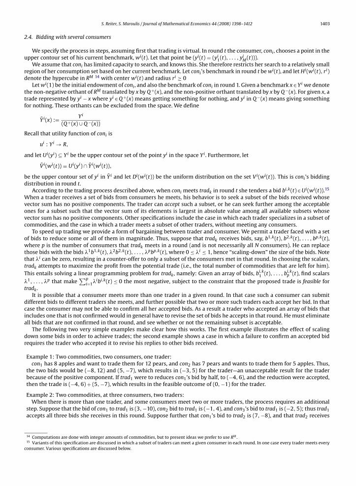
Example 1: Two commodities, two consumers, one trader:con1 has 8 apples and want to trade them for 12 pears, and con2 has 7 pears and wants to trade them for 5 apples. Thus,

the two bids would be (−8, 12) and (5, −7), which results in (−3, 5) for the trader—an unacceptable result for the traderbecause of the positive component. If trad1 were to reduces con1’s bid by half, to (−4, 6), and the reduction were accepted,then the trade is (−4, 6) + (5, −7), which results in the feasible outcome of (0, −1) for the trader.

Example 2: Two commodities, at three consumers, two traders:When there is more than one trader, and some consumers meet two or more traders, the process requires an additional

step. Suppose that the bid of con1 to trad1 is (3, −10), con2 bid to trad1 is (−1, 4), and con3’s bid to trad1 is (−2, 5); thus trad1accepts all three bids she receives in this round. Suppose further that con1’s bid to trad2 is (7, −8), and that trad2 receives

14 Computations are done with integer amounts of commodities, but to present ideas we prefer to use RM .15 Variants of this specification are discussed in which a subset of traders can meet a given consumer in each round. In one case every trader meets every

consumer. Various specifications are discussed below.

1404 S. Reiter, S. Maroulis / Journal of Mathematical Economics 44 (2008) 1398–1412

bids from other consumers such that he accepts con1’s. However, con1’s response to the acceptance of his bids by both trad1,and trad2 is to confirm his bid to trad2 and not confirm his bid to trad1. Then trad1 is left with the two confirmed bids, (−1, 4)and (−2, 5). This pair of bids is infeasible for the trader, so he must inform con1 and con2 that their bids are not accepted inthat round.

To summarize, the trading process proceeds in four steps per round: each consumer submits bids to each trader whovisited; each trader proposes a counter-offer to each consumer, in the form of a possibly scaled-down, or even empty, bid;each consumer with a non-empty counter-offer decides whether or not to confirm the proposed transaction; after receivingconfirmations or disconfirmations from all the relevant consumers, each trader decides whether to v erify the proposedtrades, checking to see if they are still f easible.

2.5. Trading structures

In addition to being either virtual or actual, trading can also take place on different trading structures. A structure involvesa number of parameters. These include:

the number of commodities;the number of consumers;the number of traders.

Meetings between traders and consumers, and traders and traders can vary in a set of patterns of contact including:

1. In each round each trader meets a random selection of consumers.2. The set of consumers is partitioned into fixed subsets; this captures the case where consumers are located in distinct

separated areas, or are part of some other partition into classes, and traders are also partitioned into groups that meetonly with designated subsets of consumers; a special case of this is a structure in which one trader meets all consumers.

3. The set of traders has a hierarchical structure; traders are placed at different levels; a trader at level 1 meets consumers;if there are traders at level 2, those traders do not meet consumers, but a level 1 trader might also meet a trader at level 2.If there are traders at level 3, they would meet traders at level 2, and so on up the levels of the hierarchy. A trader at levell who receives bids that she cannot accept can, if she meets a trader at level l + 1, transmit a subset of them – possibly theentire set – to that trader. The trader who receives those bids can accept a subset of the bids submitted, provided that thesum of the bids in that subset is a vector whose components are non-positive.

4. The set of traders are partitioned by commodities; in one case all traders deal in the same set of commodities, namely, allcommodities; in another case, each trader specializes in a single commodity which is exchanged for numeraire.

5. A combination of the structures above (e.g., hierarchical and commodity-based partitions).

In summary, the dynamic behavior of the trading process depends on whether trading is virtual or actual; the structure ofthe set of traders; the consumers and traders who meet in a given round; and each trader’s choice of his acceptance parameteryk, and the additional criterion he uses to select a subset of bids to accept. Our aim is to use computational, agent-basedmodels to study the dynamic paths and limits generated by particular specifications of such a trading process. In doing so,we acknowledge that our computational approach cannot include all possible scenarios of economic interest.16 Section 4describes in detail the structures used in our initial investigation.

3. Efficiency

The basic criterion used in economic theory for evaluating allocations of commodities is Pareto optimality. However, atcertain levels of detail other criteria are sometimes used. For instance, in evaluating the efficiency of a firm operating in amarket setting, profitability might be used as the criterion of efficiency. In studying a process of trading, one might wantto look at two things: first, how close is the result to being efficient in the sense of Pareto optimality, and second, howmuch of the traded goods are diverted from “ordinary” economic agents who participate in trading to those who operate theprocesses of trading. In our case the traders are the intermediaries through whom trade is conducted, and they might endup with positive stocks of commodities. And, because of randomness in our trading process, it is possible that trading comesto a stop while there are still possible trades that are not consumated. Moreover, because of random elements in tradingbehavior, our evaluation of the outcomes of the trading process is probabilistic.

We could in principle derive the probability distributions over outcomes that are implicitly determined by the prob-abilistic elements in the behavior of agents—the distributions that govern the selection of bids by consumers and theprobabilities that govern meetings between consumers and traders. We could then analyze the properties of the limits,

16 In the computational experiments that follow all traders deal in all commodities, and we have at most two levels of traders.

S. Reiter, S. Maroulis / Journal of Mathematical Economics 44 (2008) 1398–1412 1405

if any, to which our process converges—the Pareto optimality or other efficiency properties of the generated limits. Butin our model the commodity space is a bounded discrete set, the number of agents, their endowments of commodities,and the number of points in the set of feasible allocations are all finite. Further, the bids of each consumer are mono-tone increasing in utility. Therefore in our setting we can be sure that the limits exist. The problem is to recognize thatthe process has arrived at a limit—a state at which no further trades can take place, although continued bidding does takeplace.

If there is just one trader, the process presented here is closely related to the stochastic process of bids andacceptances presented in HRR. In HRR there is an agent – a referee – who examines the bid of each consumerin each round, and determines whether the components of the entire vector of bids add up to zero. If so, theimplied transactions take place, and the process continues with a new round of bidding. Therefore, when the envi-ronment – the commodity space, the preferences and initial endowments of consumers – is among the set ofenvironments covered by the HRR results, we can say that the limiting bidding distributions exist, and that thebenchmarks that correspond to that distribution are Pareto optimal, although the process of bidding continues indefi-nitely.

In contrast to the process in HRR, our process does not necessarily have a referee who sees all bids in each round.We can have more than one trader, and each trader might see only a proper subset of the bids made in that round.With more than one trader the situation is more complex. Nevertheless, in the process of trading, the benchmarks willgo to a limit, but without further specifications that limit is not necessarily Pareto optimal. The following example showsthis.

Suppose there are two traders, trad1 and trad2, with zero endowments of two commodities, and two consumers, con1and con2. con1 has 3 apples and no oranges, i.e., (3,0), and offers to trade 3 apples for 2 oranges, i.e., bids (−3, 2); con2has 3 oranges and no apples, i.e., (0, 3) and offers to trade 3 oranges for 2 apples, i.e., bids (2, −3). Suppose the two con-sumers meet different traders in a given round, say, con1 meets trad1 and con2 meets trad2. trad1 cannot accept con1 sbid, because he has no apples, and trad2 cannot accept con2 s bid because he has no oranges. Consequently, the limit-ing allocation is (3, 0), (0, 3), which is not Pareto optimal, because con1 prefers (0, 2) to (3, 0), and con2 prefers (2, 0) to(0, 3).

This condition can arise if, say, the two consumers are geographically, or for some other reason, separated, and the twotraders are also correspondingly separated. In such a case a third trader trad3 can be introduced, a trader who meets bothtrad1 and trad2, who ‘lay-off’ bids received that they cannot accept.

Suppose there is just one trader, trad1, who receives both bids in round 1. Then he can accept both bids; their sum is(−3, 2) + (2, −3) = (−1, −1) which is a profit of one apple and one orange for trad1, and an increase in utility for both con1and con2. The new benchmarks are: (0, 2) for con1 and (2, 0) for con2. In the case of virtual trading, the endowments remain(3, 0) for con1, (0,3) for con2 and (0,0) for trad1.

For con1 the point (1, 2) is in the upper contour set of (0, 2). Hence his bid in round 2 is (−2, 2) with positive probability.Similarly, con2 s new benchmark is (2, 0), and with positive probability con2 s bid in round 2 is (2, −2). The probability thatboth bids are made in that round is also positive. In that case trad1 receives the array of bids (−2, 2) and (2, −2). Their sumis (0, 0), so this trade is made. It results in the new holdings for con1:

(3, 0) + (−2, 2) = (1, 2)

and for con2:

(2, −2) + (0, 3) = (2, 1)

If the virtual process were to end now because we think it may have converged on a limit (perhaps because we have runthe process for a large number of rounds and observe that no further trading occurs), it is evident that this allocation of the 3apples and 3 oranges between the two consumers, with nothing left for the trader, is Pareto optimal. Within the agent-basedmodel, we can check to see if the process has indeed converged by introducing a test trader who receives the most recentbenchmarks and calculates whether there are any potential trades left to make. The test trader can also be used to evaluatethe Pareto optimality at this limit.

As a final clarifying point, note that the execution of the second virtual trade assumes that the trader does notbehave strategically in order to preserve the more beneficial outcome of (−1, −1) from the first round. While onecould certainly explore outcomes in the model where the traders misrepresent their ability to make a trade with con-sumers, the current model is based on our conception of a trader as a simple, rule-following agent facing a highlyuncertain world. Such an assumption can be defended on the grounds that the trader is an agent of an institutionthat has decided upon those rules; or alternatively that faced with the uncertainty of what the future rounds bring,the trader just accepts all trades that are feasible as they appear (e.g., the trader does not know whether accept-ing an offer that results in (0,0) in round 2, will lead to offers that result in holdings better or worse than hisholdings in round 1). It is on similar grounds that we do not include the trader in our calculations of Pareto optimal-ity.

1406 S. Reiter, S. Maroulis / Journal of Mathematical Economics 44 (2008) 1398–1412

4. Computational experiments

In this section, we report the results of computational experiments we use to investigate the properties of the tradingprocess described in Section 2. We examine two classes of cases, one with one trader and three consumers, and the otherwith 3 traders and 30 consumers; in this case the set of traders has a hierarchical structure.

4.1. One trader, three consumers

4.1.1. ParameterizationThe simulated economy consists of 3 commodities, 3 consumers, and 1 trader. The trader deals in all 3 commodities and

meets all 3 traders in every round. We note that a round does not correspond to any particular unit of time; a round is aninstance of contact between a trader and a specified number of consumers.

Initial endowments for the consumers were assigned randomly at the beginning of the simulation; each consumer wasgiven n of each good, where n is a random draw from the uniform distribution on the interval [1, 4] in the set of integers.

Consumer bidding takes place exactly as discussed in Section 2.4. All points in the consumer’s upper contour set have anequal probability of being chosen, and we set the radius, ri, of hypercube, Hi(wi(t), ri) equal to 2. We consider four possibleutility functions that underlie the behavior of consumers:

• Cobb-Douglas utility functions, given by17:

u1(x1, y1, z1) = x˛11 yˇ1

1 z�11

u2(x2, y2, z2) = x˛22 yˇ2

2 z�22

u3(x3, y3, z3) = x˛33 yˇ3

3 z�33

• Utility functions in which the three commodities are pure complements, given by:

u1(x, y, z) = u2 = u3 = min{x, y, z}

• The utility functions used in Scarf’s example – a special case of pure complements – given by:

u1(x1, y1, z1) = min{x1, y1}u2(x2, y2, z2) = min{x2, z2}u3(x3, y3, z3) = min{y3, z3}

• Non-concave utility functions, given by:

u1(x1, y1, z1) = ˛1x1 + ˇ1y1 + �1(z1)2

u2(x2, y2, z2) = ˛2x2 + ˇ2z2 + �2(y2)2

u3(x3, y3, z3) = ˛3y3 + ˇ3z2 + �3(x3)2

Such functions can result in disconnected upper contour sets. For instance, in the conventional two-person EdgeworthBox graphic, a given point represents an allocation of the two goods between the two agents, the intersection of thetwo upper contour sets is a lens-shaped area. When preferences are not convex, that intersection can consist of severallens-shaped regions that alternate between being in the upper contour set, and being in the lower contour set.

Trader behavior takes place as described in Section 2 with one exception. In the three-consumer case, the bargainingbehavior between consumer and trader introduced to speed up trading is not necessary. The trader’s acceptance parameter,yk, is set to zero.

4.1.2. Virtual tradingTable 1 shows the results of 100 runs of this trading structure under the virtual trading regime. Each run consists of 10,000

rounds instances of contact—between a trader and the set of 3 consumers.

17 In cases where there are only three consumers: ˛1 = ˇ2 = �3 = 0.495; ˛3 = ˇ1 = �2 = 0.33; ˛2 = ˇ3 = �1 = 0.175.

S. Reiter, S. Maroulis / Journal of Mathematical Economics 44 (2008) 1398–1412 1407

Table 1Summary of 1 trader, 3 consumer results (virtual trading, 10,000 rounds)

Utility Fn N Conv. U. limit Conv. time Pareto Opt Pct profit

Cobb-Douglas 92 69 69 3.14 68 0Pure Compl. 70 70 5 10.4 67 0.60Scarf 100 83 9 11.4 79 0.45Non-Concave 100 95 95 6.38 93 0

N, Number of total runs. Runs with initial endowments with zero potential trades are not included. Conv., Number of runs that converged to a limit. U.limit, Number of runs that converged to a limit of one repeated trade, as opposed to cycling through a set of trades. Conv. time, Mean number of trades toconvergence. Pareto Opt, Number of runs that converged to a limit that is Pareto optimal (assuming that the trader does not re-contribute any profit). PctProfit, Mean percentage of total goods captured by the trader.

Fig. 1. Distribution of final trader profit across convergent runs (virtual trading).

• N represents the number of runs for a given utility function.18

• The ‘Convergence’ column shows the subset of N runs that converged to a limit. Convergence is determined by enumeration(there are only three consumers). Given each consumer’s utility function we are able to examine all possible combinationsof potential trades that remain after the run concludes.

• ‘Unique Limit’ denotes the subset of N runs that resulted in a limit that consists of only one possible trade.• ‘Convergence Time’ is the average number of trades (not rounds) it took for the process to converge to its limit, averaged

across all convergent runs for a given utility function.• The ‘Pareto Opt’ column lists the number of runs for which the final holdings of goods could not be rearranged in a

manner that increased the utility of one consumer, without decreasing the utility of another. Because there are only threeconsumers, this determination is made by enumerating all remaining trading options available after convergence.19

• The final column, ‘Pct Profit,’ reports a crude indicator of trader profit—the percentage of total commodities captured bythe trader in the last round of the virtual trading process.20

For example, Table 1 shows that for the trading structure using the Cobb-Douglas utility specification, 92 of the 100 runswere initialized with consumer endowments that permitted trading, 69 of those 92 runs converged within 10,000 rounds,each of the 69 runs converged to a unique limit, and 68 of the 69 converged to a Pareto optimal point. On average across the92 runs, it took 3.14 trades before the process converged.

The first thing to note about the virtual trading results is that the process most often converges to a stable limit. With theCobb-Douglas and Non-Concave utility functions, this limit always turned out to be unique; the process reaches a point afterwhich consumers engage in the same trade over and over. In the cases of the Scarf and Pure Complement utility functions,the limit is often not unique; instead the consumers cycle through several trades, all of which result in identical utilities.

The second thing to note about the virtual trading results is that a large fraction of the converged runs resulted in finalholdings that can be characterized as Pareto optimal: 68 of the 69 converged runs for the Cobb-Douglas utility specificationare Pareto optimal, 79 of the 83 converged runs for the Scarf utility function are Pareto optimal, 67 of the 70 converged runsfor the Pure Complements utility function are Pareto optimal, and 93 of the 95 converged runs for the Non-Concave utilityfunction are Pareto optimal.

The percentage of the total quantities of all commodities captured by the trader in the virtual exchange process is a roughmeasure or indicator of the cost of operating the process. The mean percentage across all convergent runs is listed Table 1,and the distribution of trader profit across all convergent runs is shown in Fig. 1. The most frequent outcome for the traderunder the Scarf and Pure Complement utility functions is zero commodities; for the Cobb-Douglas and Non-Concave utility

18 Sometimes the actual number of runs executed is less than 100, because initial endowments are randomly distributed across consumers and soinitializations of trading structures can sometimes result is situations in which trading is not feasible.

19 We should note that if the process resulted in profit for the trader, the goods that constitute the traders profit were not returned to the consumersbefore testing for Pareto optimality. In this sense, the trader could not be made worse off either.

20 The profit of the last round of trading is the relevant round to examine in the case of virtual trading, as the previous rounds do not result in any realexchange of goods.

1408 S. Reiter, S. Maroulis / Journal of Mathematical Economics 44 (2008) 1398–1412

Fig. 2. Trader profit over time (virtual trading).

functions, zero commodities is the only outcome in all the runs (and subsequently not depicted in Fig. 1). However, there aredifferent paths to the final profit distributions for each utility function. Examining the average profit over time as illustratedin Fig. 2, we see that the average profit converges to zero in the case of the Cobb-Douglas and Non-Concave utility functions.For the Pure Complement and Scarf functions, the average profit decreases rapidly at first, but its variability grows over time.

4.1.3. Actual tradingThe results for the case of actual trading are presented in the same format as those for virtual trading, and the results are

similar. Table 2 shows that the actual trading runs are characterized by frequent convergence to a Pareto optimal outcome.There are three notable differences from the outcomes in the case of virtual trading.

• One is that the convergence seems to be faster in the case of actual trading, especially for the Pure Complement and Scarfutility functions.

• A second difference is that the trader’s profit is much higher with actual trading, as measured by the percentage of thetotal commodities that are accumulated by the trader during the process.

• Finally, Fig. 3 illustrates trader profit over time averaged across the all the convergent runs. In the case of virtual trading,we saw the variability of the average profit grow over time, whereas in the case of actual trading we see a smooth andsteady convergence to zero.

4.2. A hierarchical structure of traders

4.2.1. ParameterizationIn this trading structure we have 3 commodities, 30 consumers, three level 1 traders, and two level 2 traders. Level 1 and

level 2 traders each deal in all three commodities. Consumers are divided into three mutually exclusive subsets of 10. At thebeginning of the simulation, each level 1 trader is assigned one subset of ten consumers whom she meets every round. Thelevel 2 trader meets all three level 1 traders in every round, but has no direct encounters with consumers.

The trader acceptance parameter, yk, is set to zero for both level 1 and level 2 traders. To speed up trading, level 1 andlevel 2 traders faced with a set of bids are permitted to respond to consumer bids with counter-offers that reduce the bidsin magnitude, as described in detail in Section 2.4. All trading is virtual.

Table 2Summary of 1 trader, 3 consumer results (actual trading, 10,000 rounds)

Utility Fn N Conv. U. limit Conv. time Pareto Opt Pct Profit

Cobb-Douglas 87 83 83 2.79 83 1.83Pure Compl. 73 73 6 1.78 73 16.0Scarf 100 100 36 4.49 100 15.3Non-Concave 100 7 97 4.09 97 12.9

S. Reiter, S. Maroulis / Journal of Mathematical Economics 44 (2008) 1398–1412 1409

Fig. 3. Trader profit over time (actual trading).

Table 3Summary of 4 trader, 30 consumer results (actual trading, 2000 rounds, 100 runs)

Utility Fn Initial potential trades Final potential trades Total trades

Cobb-Douglas 6010 50.7 49.6Pure Compl. 24,600 263 725Scarf 64,600 91.9 439Non-Concave 147,000 25.6 54.9

Initial potential trades: Number of potential trades two-way trades at time period 0. Final potential trades: Number of potential trades two-way trades attime period 2000. Total trades: Mean number of trades executed by the traders.

For consumer bidding, we consider the same four types of utility functions as in Section 4.1.1, but with two differences toaccount for the increase in consumers. More specifically, the exponents in the Cobb-Doug utility functions and the coefficientsin the non-concave utility functions are determined for each consumer by random draws from the uniform distribution onthe interval [0, 1] (and no longer necessarily add up to 1), resulting in a heterogeneous populations of agents. In the Scarfcase, the utility functions are distributed uniformly across the population, with each of the Scarf utility functions is assignedto 10 consumers. As in the three consumer scenario, initial endowments for each consumer are determined by a randomdraw from the uniform distribution on the integers in the interval [0, 4].

4.2.2. ResultsWith 30 consumers, enumerating all possible trading scenarios is not feasible. We do not have the computational power

needed to investigate all trading possibilities between consumers. Consequently, we are only able to take a snapshot of theprocess at a few points in time, and see whether the process is moving in the direction of convergence and efficiency. In thissection, we present those snapshots.

Table 3 shows the results of 100 runs of the nested-trader structure for virtual trading. Each run consists of 2000 rounds.Table 3 shows that, at least on one measure, the process is headed towards convergence. The first column shows the number ofpotential pair-wise trades between the consumers at the beginning of the simulation—a measure we were able to calculateby enumeration. The second column shows, for all four utility specifications, that after 2000 rounds the total number ofpossible pair-wise trades has decreased by at least two orders of magnitude.

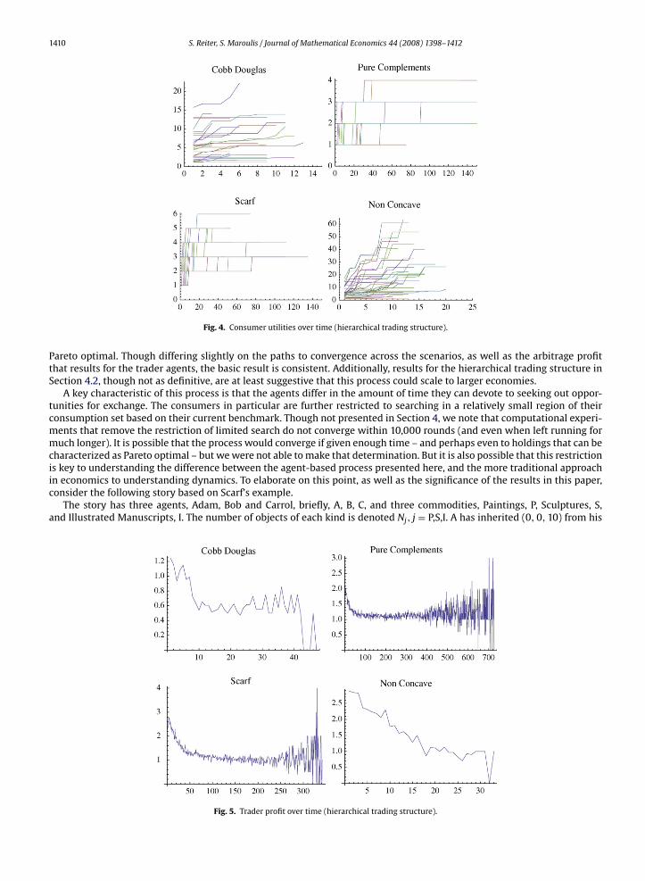
Fig. 4 plots the utility over time for all 30 consumers. The x-axis records only time periods in which a trade occurred, they-axis the utility level of a consumer. As one would expect of a process moving towards an efficient outcome, Fig. 4 shows aclear trend of increasing consumer utility levels.

Fig. 5 shows average trader profit over time. This measure follows a pattern similar to Virtual Trading under the three-consumer specifications of the model. In particular, we see a rapid initial decrease in average profit, followed by an increasein variability for the Pure Complement and Scarf utility functions.

5. Discussion

The basic finding in the three consumer, one trader results in Section 4.1 is the stochastic process of exchange presentedhere quite frequently converges to a limit, and most often the holdings of consumers at that limit can be characterized as

1410 S. Reiter, S. Maroulis / Journal of Mathematical Economics 44 (2008) 1398–1412

Fig. 4. Consumer utilities over time (hierarchical trading structure).

Pareto optimal. Though differing slightly on the paths to convergence across the scenarios, as well as the arbitrage profitthat results for the trader agents, the basic result is consistent. Additionally, results for the hierarchical trading structure inSection 4.2, though not as definitive, are at least suggestive that this process could scale to larger economies.

A key characteristic of this process is that the agents differ in the amount of time they can devote to seeking out oppor-tunities for exchange. The consumers in particular are further restricted to searching in a relatively small region of theirconsumption set based on their current benchmark. Though not presented in Section 4, we note that computational experi-ments that remove the restriction of limited search do not converge within 10,000 rounds (and even when left running formuch longer). It is possible that the process would converge if given enough time – and perhaps even to holdings that can becharacterized as Pareto optimal – but we were not able to make that determination. But it is also possible that this restrictionis key to understanding the difference between the agent-based process presented here, and the more traditional approachin economics to understanding dynamics. To elaborate on this point, as well as the significance of the results in this paper,consider the following story based on Scarf’s example.

The story has three agents, Adam, Bob and Carrol, briefly, A, B, C, and three commodities, Paintings, P, Sculptures, S,and Illustrated Manuscripts, I. The number of objects of each kind is denoted Nj, j = P,S,I. A has inherited (0, 0, 10) from his

Fig. 5. Trader profit over time (hierarchical trading structure).

S. Reiter, S. Maroulis / Journal of Mathematical Economics 44 (2008) 1398–1412 1411

father, who was a passionate collector of I; B has inherited (0, 10, 0) from his father, who was a passionate collector of S; C hasinherited (10, 0, 0) from her father, who was a passionate collector of P. A collects paintings and sculpture, and has no interestin illuminated manuscripts; B collects paintings and illuminated manuscripts, and has no interest in sculpture; C collectssculpture and illuminated manuscripts, and has no interest in paintings. Moreover, each collector wants his collection toconsist of matched pairs of the objects he collects, to be displayed together. Thus, their utility functions are as follows:

uA(NP, NS, NI) = min{NP, NS}uB(NP, NS, NI) = min{NP, NI}uC(NP, NS, NI) = min{NS, NI}

Using the traditional approach to studying dynamics to analyze this scenario, one would derive the demand functionsand study the differential equations that represents price adjustment. Scarf showed that on a example such as this, the pathsgenerated are closed orbits. Thus, prices do not converge and allocations do not converge to a Pareto optimum.

Our process is different from this traditional approach in at least two ways. First, our process introduces into this examplea dealer, D, who trades art objects, and who visits the three collectors from time to time. When a collector, say A, meets D, Aproposes an exchange. Because A gets no satisfaction from I, he proposes trading some of his endowment of I for paintingsand sculptures. Because Paintings and Sculptures are strict complements for him, he proposes to accept an equal number ofthem, say, one painting and one sculpture, in exchange for some illuminated manuscripts. The Dealer would in any singleround of visits to the collectors accept a triple of bids if and only if the sum of the bids provides him with at least zero profit.

Second, our process also introduces into this example a limited search capacity of for the consumers. Interestingly, thisrestriction ensures “sensible” behavior for the consumers, in the following sense. Note that A gets no direct satisfaction fromI; but whether A is aware of it or not, he could trade units of I for units of P and S. Therefore, A would be prudent to offer asmall amount, say one or two units of I in exchange for a pair consisting of a unit of P and a unit of S.

In the computed trading runs that represent this story in Section 4, whether or not the consumers behave “sensibly”affects the outcomes. If the three consumers behave in a way that is “sensible,” given their endowments, preferences andinformation about the trading process, then the process converges to a Pareto optimal allocation. On the other hand, if anagent were to allowed to search for bids much further from his current benchmark – for instance, bid his entire endowmentof the one good he does not value for one unit of the pair of the goods he values – we were not able to reach convergencein our simulations even when allowing the process to run for over 100,000 rounds. Of course, we cannot claim that withoutlimiting the search capacity of the consumer, that the process will not converge eventually (and even on a Pareto optimaloutcome); but at the very least we can say the bounded search capacity of the agents seems to have unexpected benefitsfor a decentralized process of exchange. An interesting avenue for future work could involve adding more “intelligence” tothe agents, and examining the impact of such modifications on both convergence and efficiency. This could include allowingthe agents to search more intelligently for bids through a process of learning, as well as permitting strategic behavior on thepart of both the consumers and traders.

6. Conclusion

In this paper, we attempt to address a longstanding gap in economic theory—the gap between claims for the dynamicefficiency of markets found in introductory textbooks, and the findings of formal economic theory which has been ableto defend this claim only under rather restrictive assumptions. We present a process of exchange based on ideas that alsounderlie the B process – a decentralized and stochastic process of trading proposed by Hurwicz, Radner, and Reiter over threedecades ago – and explore its properties through the use of agent-based computation. We demonstrate that a decentralizedprocess can find efficient outcomes in economies with multiple agents and three-commodities, economies in cases that rangefrom traditional Cobb-Douglas utility functions, to cases like the Scarf example that have historically posed problems foreconomic theory. Our hope is that we illustrate an alternative to the classical excess demand dynamics of price adjustmentsthat can provide the basis for future work in this direction.

References

Arrow, K., 1951. An extension of the basic theorems of classical welfare economics. In: Neyman, J. (Ed.), Proceedings of the Second Berkeley Symposium onMathematical Statistics and Probability. University of California Press, pp. 502–532.

Arrow, K., Hurwicz, L., 1958. On the stability of the competitive equilibrium I. Econometrica 26, 522–552.Arrow, K., Hurwicz, L., 1960. Competitive stability under weak gross substitutability: the “euclidean distance” approach. International Economic Review 1,

38–49.Bala, V., 1988. Computer simulation of B-processes. Working Paper 410. Cornell University, Department of Economics.Debreu, G., 1959. Theory of value. In: An Axiomatic Analysis of Economic Equilibrium. John Wiley and Sons, Inc., New York.Hahn, F., 1982. Stability. In: Arrow, K., Intriligator, M. (Eds.), In: Handbook of Mathematical Economics, vol. 2. North-Holland Publishing Company, Chapter

14.Hurwicz, L., Radner, R., Reiter, S., 1975a. A stochastic decentralized resource allocation process: part 1. Econometrica 43, 187–221.Hurwicz, L., Radner, R., Reiter, S., 1975b. A stochastic decentralized resource allocation process: part 2. Econometrica 43, 363–394.Joosten, R., Talman, A., 1993. A simplicial variable dimension restart algorithm to find economic equilibria on the unit simplex using n(n + 1)rays. Tech. Rep.

Report M 93-01. Department of Mathematics, Maastricht University, Maastricht.Jordan, J., 1987. The informational requirement of local stability in decentralized allocation mechanisms. In: Groves, T., Radner, R., Reiter, S. (Eds.), Information,

Incentives and Economic Mechanism, Essays in Honor of Leonid Hurwicz. University of Minnesota Press.

1412 S. Reiter, S. Maroulis / Journal of Mathematical Economics 44 (2008) 1398–1412

Kuhn, H., 1968. Simplicial approximation of fixed points. In: Proceedings of the National Academy of Sciences, p. 61.Matsui, T., 1981. A stochastic adjustment process for nonconvex and indecomposable environments. Ph.D. dissertation. University of Minnesota, Minneapolis.Miller, J.H., Page, S.E., 2007. Complex Adaptive Systems: An Introduction to Computational Models of Social Life. Princeton University Press.Reiter, S., 1959. A market adjustment mechanism. Institute Paper 1. School of Industrial Management, Purdue University, West Lafayette, Indiana.Reiter, S., 1981. A dynamic process of exchange. In: Horwich, G., Quirk, J.P. (Eds.), Essays in Contemporary Fields of Economics. Purdue University Press.Saari, D., Simon, C., 1978. Effective price mechanisms. Econometrica 46, 1097–1125.Samuelson, P., 1941. The stability of equilibrium: comparative statics and dynamics. Econometrica 9, 97–120.Samuelson, P., 1942. The stability of equilibrium: linear and nonlinear systems. Econometrica 10, 1–25.Samuelson, P., 1947. Foundations of Economic Analysis. Harvard University Press.Scarf, H., 1960. Some examples of global instability of competitive equilibrium. International Economic Review 1, 157–172.Shafer, W., Sonnenschein, H., 1982. Market demand and excess demand functions. In: Arrow, K.J., Intriligator, M. (Eds.), Handbook of Mathematical Economics.

Vol. 2 of Handbook of Mathematical Economics. North-Holland Publishing Company, Chapter 14.Shapley, L., Shubik, M., 1977. Trade using one commodity as a means of payment. Journal of Political Economy 85, 937–968.Smale, S., 1976a. A convergent process of price adjustment and global Newton methods. Journal of Mathematical Economics 3 (1), 1–14.Smale, S., 1976b. Exchange processes with price adjustment. Journal of Mathematical Economics 3, 211–226.Sonnenschein, H., 1972. Market excess demand functions. Econometrica 40, 549–563.Sonnenschein, H., 1973. Do Walras’ identity and continuity characterize community excess demand functions? Journal of Economic Theory 6, 345–354.Walras, L., 1874. Elements d’economie politique pure (L. Corbaz, Lausanne). Elements of Pure Economics. Allen and Unwin, London (English translation by

W. Jaffe, 1954).Wilensky, U., 1999. NetLogo. Center for Connected Learning and Computer-Based Modeling. Northwestern University, Evanston, IL (http://ccl.northwestern.

edu/netlogo/).