JOURNAL OF LA P-ODN: Prototype based Open Deep Network for ...

JOURNAL OF LATEX CLASS FILES, VOL. 14, NO. 8, AUGUST 2015 1

P-ODN: Prototype based Open Deep Network forOpen Set Recognition

Yu Shu, Yemin Shi, Yaowei Wang, Member, IEEE, Tiejun Huang, Senior Member, IEEE, Yonghong Tian, SeniorMember, IEEE

Abstract—Most of the existing recognition algorithms areproposed for closed set scenarios, where all categories are knownbeforehand. However, in practice, recognition is essentially anopen set problem. There are categories we know called “knowns”,and there are more we do not know called “unknowns”. Enumer-ating all categories beforehand is never possible, consequentlyit is infeasible to prepare sufficient training samples for thoseunknowns. Applying closed set recognition methods will naturallylead to unseen-category errors. To address this problem, wepropose the prototype based Open Deep Network (P-ODN) foropen set recognition tasks. Specifically, we introduce prototypelearning into open set recognition. Prototypes and prototyperadiuses are trained jointly to guide a CNN network to derivemore discriminative features. Then P-ODN detects the unknownsby applying a multi-class triplet thresholding method based onthe distance metric between features and prototypes. Manuallabeling the unknowns which are detected in the previous processas new categories. Predictors for new categories are added tothe classification layer to “open” the deep neural networks toincorporate new categories dynamically. The weights of newpredictors are initialized exquisitely by applying a distancesbased algorithm to transfer the learned knowledge. Consequently,this initialization method speed up the fine-tuning process andreduce the samples needed to train new predictors. Extensiveexperiments show that P-ODN can effectively detect unknownsand needs only few samples with human intervention to recognizea new category. In the real world scenarios, our method achievesstate-of-the-art performance on the UCF11, UCF50, UCF101 andHMDB51 datasets.

Index Terms—Open set recognition, prototype based OpenDeep Network, P-ODN, action recognition.

I. INTRODUCTION

DEEP neural networks have demonstrated significant per-formance on many visual recognition tasks [1]–[3]. Al-

most all of them are proposed for closed set scenarios, whereall categories are known beforehand. However, in practice,

Manuscript received March 19, 2019. This work is partially supportedby grants from the National Key R&D Program of China under grant2017YFB1002401, the National Natural Science Foundation of China undercontract No. U1611461, No. 61390515, No. 61425025, No. 61471042 and No.61650202, also supported by grants from NVIDIA and the NVIDIA DGX-1AI Supercomputer.

Corresponding author: Yonghong Tian (email: [email protected]) andYaowei Wang (email: [email protected]).

Y. Shu is with School of Academy for Advanced Interdisciplinary Studies,Peking University, Beijing 100871, China, with the National Engineering Lab-oratory for Video Technology, China, and with the Peng Cheng Laboratory,China.

Y. Shi, T. Huang and Y. Tian are with the National Engineering Laboratoryfor Video Technology, School of EE&CS, Peking University, Beijing 100871,China and with the Peng Cheng Laboratory, China.

Y. Wang is with School of Information and Electronics, Beijing Instituteof Technology, Beijing, China and with the Peng Cheng Laboratory.

Fig. 1. Open Set Recognition. The training set contains sufficient labeledsamples of different categories (colored in green and blue), while the testingset contains knowns but also unknowns which haven’t been seen at all.The solution should be able to accept the knowns and reject the unknowns.Simultaneously, the solution should classify knowns into correct knowncategories and further be able to classify unknowns as well.

some categories can be known beforehand, but more categoriescan not be known until we have seen them. We call thecategories we know as priori the “knowns” and those wedo not know beforehand the “unknowns”. Enumerating allcategories is never possible for the incomplete knowledgeof categories. And preparing sufficient training samples forall categories beforehand is time and resource consuming,which is also infeasible for unknowns. Consequently, applyingclosed set recognition methods in real scenarios naturally leadsto unseen-category errors. Therefore, recognition in the realworld is essentially an open set problem, and an open setmethod is more desirable for recognition tasks.

As shown in Fig. 1, in open set recognition problem,categories of the training set have sufficient labeled samples,which are knowns, while the testing set contains both knownsand unknowns. The solution to the problem should be able toaccept and classify knowns into correct known categories andalso reject unknowns. Simultaneously, it is natural to furtherextend to perform recognition of unknowns as shown in theright part of Fig. 1 with different color boxes classifying theunknowns.

Technically speaking, many methods on incremental learn-ing can be used to handle new instances of known categories[4]–[8]. However, most of these approaches do not considerabout unknowns or dynamically adding new categories tothe system. In [9], a discriminative metric is learned forNearest Class Mean (NCM) classification on the knowns,and new categories are added according to the mean fea-tures. This approach, however, assumes that the number ofknown categories is relatively large. An alternative multi-classincremental approach based on least-squares SVM has beenproposed by Kuzborskij et al. [10] where for each category

arX

iv:1

905.

0185

1v1

[cs

.CV

] 6

May

201

9


a decision hyperplane is learned. However, in this way, everytime a category is added, the whole set of the hyperplaneswill be updated again, which is too expensive as the numberof categories growing.

In particular, most of the researches on open set recogni-tion focus on detecting unknowns only, recent works [11]–[13] have established formulations of classifying knowns andrejecting unknowns. While it is natural to extend to classifyunknown samples after detecting unknowns. And in the realworld, solutions which further classify the unknowns are morechallenging and have a wider range of applications. Abhijit etal. [14] proposed a SVM-based recognition system that couldcontinuously recognize new categories in an open world modelby extending the NCM-like algorithms [15] to a Nearest Non-Outlier (NNO) algorithm. But it is not applicable in deepneural networks, and the performance is much worse thandeep neural network based algorithms. Recently, in the work[16], Yang et al. have tried to handle the open set recognitionproblem by training prototypes to represent the unknowns. Butthe solution works on the assumption that all unknowns havesufficient labeled samples to train discriminative prototypes,which is not realistic. And the system needs to be retrainedwhen new categories comes, which is time and computationalresource consuming.

In our previous work [17], we proposed an Open DeepNetwork (ODN) algorithm for open set recognition. First,we train a CNN network to classify the knowns which havesufficient samples. Then the triplet threshold of each categoryis calculated based on the correctly classified features oftraining set. Unknowns can be detected by applying the tripletthresholds on the features derived by the CNN. Manual label-ing the unknowns which are detected in the previous process,and predictors of the classification layer are added dynamicallyto incorporate new categories. Weights of the new predictorsare initialized by applying the emphasis initialization methodwhich transfers the learned knowledge of the CNN to speedup the fine-tuning. However, the triplet thresholds are calcu-lated on the sampled features of training set, consequently,unknowns detection process might be affected by the outliersof training set. Besides, relations of categories are defined onthe feature scores in emphasis initialization method, which isa simple way to estimate the similarity of categories.

Note that we will give a brief illustrations of the methodsproposed in our previous work [17] later. Specifically, thetriplet thresholding unknown detecting method will be detailedin Sec. IV-C, and the emphasis initialization method will bedetailed in Sec. IV-D.

Most recently, the prototype learning was introduced toimprove the robustness of CNNs. Yang et al. proposed the CPLto improve the robustness by using prototypes and proposedthe PL (prototype loss) to improve the intra-class compactnessand inter-class distance of the feature representation in thework [16]. Yang et al. also introduced a method to handleopen set recognition problem by using prototypes in theirpaper. However, as mentioned before, this method assumesthat samples of unknowns are sufficient to train the prototypes.And when new unknowns come, the system needs to beretrained again. Inspired by the prototype learning concept, we

propose the prototype based Open Deep Network (P-ODN) tohandle the open set recognition problem.

In this paper, we propose P-ODN to improve the robustnessin detecting unknowns and updating deep neural networks,consequently facilitating open set recognition. Basically, proto-types and prototype radiuses are trained jointly to derive moreprecise features to better represent categories. In prototypemodule, prototypes are taught to learn the centers of knowns.And in prototype radius module, values of prototypes arefurther restricted to a curtain range by learning a radius foreach category as a regularization item of prototypes. Bothof the modules help to improve the intra-class compactnessand inter-class distance of the feature representation. Thenthe correctly classified features of training set are projectedinto a different feature space by calculating the distancedistribution between the features and prototypes. The tripletthresholds are learned based on the correctly classified distancedistribution. Instead of detecting unknowns directly on thefeatures, based on the statistic information of training samples,detecting unknowns based on the distance of prototypes keepsknowledge of the model, which has less potential to be effectedby the outliers of training set. After manual labeling theunknowns which are detected in the previous process, newpredictors are initialized based on the distance distributionof new samples and prototypes. Each weight column of theknowns is integrated to initialize the new weight according tothe distance distribution. And the distance distribution containsmore robust relation knowledge of the new category andknowns. Finally, fine-tuning the model with the manual labeledsamples to incorporate new categories.

In order to give a convincing results of our P-ODN, inthis paper, we choose to focus on the action recognitionproblem which is a more challenging recognition task. Theeffectiveness of the proposed framework is evaluated on fourpublic datasets: UCF11, UCF50, UCF101 and HMDB51. Theexperimental results show that our method can effectivelydetect unknowns and needs only few samples with humanintervention to recognize a new category. And our methodachieves the state-of-art performance on all the four datasetsin real world scenarios.

The remainder of this paper is organized as follows. Sec.II simply reviews the related works on incremental learning,open set learning and action recognition. Sec. III gives anoverview of prototype based Open Deep Network (P-ODN).And the specific algorithms of P-ODN are presented in Sec.IV. The experimental results are discussed in Sec. V. Finally,Sec. VI concludes this paper.

A preliminary version of this work has been publishedin [17]. The main extensions include four aspects. First, weintroduce the prototype learning into open set recognitiontasks. In order to learn more discriminative features, we trainthe prototype and the prototype radius of each category jointlyby applying the prototype module and the prototype radiusmodule. Second, the triplet thresholding method is extendedto detect unknowns based on the distance metric betweenfeatures and prototypes, which is more robust. Third, weextend the Emphasis initialization method to a distances basedweights initialization method to consider relations between


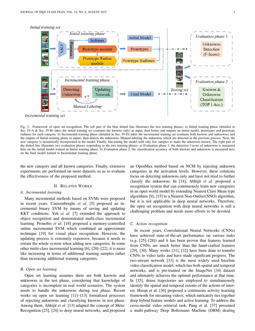
Fig. 2. Framework of open set recognition. The left part of the blue dotted line illustrates the two training phases: a) Initial training phase (detailed inSec. IV-A & Sec. IV-B) takes the initial training set (contains the knowns only) as input, then learns and outputs an initial model, prototypes and prototyperadiuses for each category. b) Incremental training phase (detailed in Sec. IV-D) takes the incremental training set (contains both knowns and unknowns) andthe outputs of Initial training phase as inputs, then detects the unknowns. Manual labeling the unknowns which are detected in the previous process. Next, thenew category is dynamically incorporated in the model. Finally, fine-tuning the model with only few samples to make the unknowns known. The right part ofthe dotted line illustrates two evaluation phases responding to the two training phases: a) Evaluation phase 1, the detection f-score of unknowns is measuredhere on the initial model trained in Initial training phase. b) Evaluation phase 2, the classification accuracy of both knowns and unknowns is measured hereon the final model trained in Incremental training phase.

the new category and all known categories. Finally, extensiveexperiments are performed on more datasets so as to evaluatethe effectiveness of the proposed method.

II. RELATED WORKS

A. Incremental learning

Many incremental methods based on SVMs were proposedin recent years. Cauwenberghs et al. [5] proposed an in-cremental binary SVM by means of saving and updatingKKT conditions. Yeh et al. [7] extended the approach toobject recognition and demonstrated multi-class incrementallearning. Pronobis et al. [18] proposed a memory-controlledonline incremental SVM which combined an approximatetechnique [19] for visual place recognition. However, theupdating process is extremely expensive, because it needs toretrain the whole system when adding new categories. In someother multi-class incremental learning [6], [20]–[22], it is morelike increasing in terms of additional training samples ratherthan increasing additional training categories.

B. Open set learning

Open set learning assumes there are both knowns andunknowns in the test phase, considering that knowledge ofcategories is incomplete in real world scenarios. The systemneeds to handle the unknowns during test phase. Recentworks on open set learning [11]–[13] formalized processesof rejecting unknowns and classifying knowns in test phase.Among them, Abhijit et al. [13] adapted the concept of Meta-Recognition [23], [24] to deep neural networks, and proposed

an OpenMax method based on NCM by rejecting unknowncategories in the activation levels. However, these solutionsfocus on detecting unknowns only and have not tried to furtherclassify the unknowns. In [14], Abhijit et al. proposed arecognition system that can continuously learn new categoriesin an open world model by extending Nearest Class Mean typealgorithms [9], [15] to a Nearest Non-Outlier(NNO) algorithm,but it is not applicable in deep neural networks. Therefore,the open set recognition with deep neural networks is still achallenging problem and needs more efforts to be devoted.

C. Action recognition

In recent years, Convolutional Neural Networks (CNNs)have achieved state-of-the-art performance on various tasks(e.g. [25]–[28]) and it has been proven that features learnedfrom CNNs are much better than the hand-crafted features[29], [30]. Many works [31], [32] have been done to transferCNNs to video tasks and have made significant progress. Thetwo-stream network [33] is the most widely used baselinevideo classification model, which has both spatial and temporalnetworks, and is pre-trained on the ImageNet [34] datasetand ultimately achieves the optimal performance at that time.In [35], dense trajectories are employed to simultaneouslyidentify the spatial and temporal extents of the actions of inter-est. Hasan et al. [36] proposed a continuous activity learningframework for streaming videos, which intricately ties togetherdeep hybrid feature models and active learning. To address thecross-modal video retrieval task, Pang et al. [37] presenteda multi-pathway Deep Boltzmann Machine (DBM) dealing


with low-level features of various types. Later, some peoplesuccessfully trained ultra-deep video classification networks.Wang et al. [2] adopted very deep ConvNet architectures [38],[39] to unleash the full potential of temporal segment networkframework. The latest works [2], [40] have achieved fantasticperformance. However, these works are designed for a staticclosed world, how to open the deep neural networks and howto dynamically handle unknowns still remain unsolved.

III. OVERVIEW

The framework of our open set recognition approach isshown in Fig. 2. Two training phases and two evaluationphases constitute the whole framework. The initial training setwhich contains only knowns is provided to the Initial trainingphase (detailed in Sec. IV-A & Sec. IV-B) as input. Then aninitial model is trained, as well prototypes and prototype ra-diuses of categories. The Incremental training phase (detailedin Sec. IV-D) takes the incremental training set (contains bothknowns and unknowns) as input and extracts the features byusing the initial model. Then distances of the features and theprototypes are measured under the constraint of the prototyperadiuses. Next, a triplet thresholding method proposed in ourprevious work [17] is modified to apply in our framework todetect the unknowns. Manual labeling the unknowns as newcategories which are dynamically incorporated in the model.Then fine-tuning the model with only few samples to make theunknowns known. Finally, the final output model can classifyboth knowns and unknowns.

Two evaluation phases are set to evaluate the model per-formance. Evaluation phase 1 is carried out after the Initialtraining phase. Testing set which contains both knowns andunknowns is provided to the initial model, and we measurethe detection f-score of unknowns at this phase. Evaluationphase 2 is carried out after the Incremental training phase.Classification TOP 1 accuracy of both knowns and unknownsis measured here as the most important performance indicatorof open set recognition tasks.

IV. PROTOTYPE BASED OPEN DEEP NETWORK

The structure of prototype based open deep network (P-ODN) in the Initial training phase is shown in Fig. 3. Basically,this phase includes two major modules: first, a Prototypemodule is applied to learn prototypes of categories based onthe prototype learning. Second, in order to guarantee eachprototype of the category in a certain range, a Prototype Radiusmodule is proposed. Each category will learn a prototyperadius to further restrict the scope of features derived by themodel. Three kinds of losses are applied to train prototypesand prototype radiuses. First we apply the cross entropy loss totrain the classification capacity of the neural networks, whichwe denotes as loss1:

loss1 = − 1

S

S∑i=1

[labeli ∗ log(softmax(fi))] (1)

where S is the batch size, fi is the feature of the ith sample inthe batch, and labeli is the ground truth. Second, the prototype

loss, which is firstly proposed by [16], is modified to apply inour framework to train the prototypes of knowns. Third, wepropose the prototype radius loss, which guides the model tolearn the radius scope of each known category. Note that theprototype loss and the prototype radius loss will be introducedin details in Sec. IV-A and Sec. IV-B later.

The Initial training phase outputs the initial model, trainedprototypes and prototype radiuses, and they will be used laterin the Incremental training phase.

Major modules (Detecting Unknowns and Updating Net-work) of P-ODN in the Incremental training phase are shownin Fig. 2. The initial model trained in the Initial training phaseextracts the features of the incremental training set here. InSec. IV-C, we will simply review a triplet thresholding methodof unknowns detection that proposed in our previous work[17]. Then the method is modified to be applicable in the P-ODN to detect the unknowns based on the distance metric ofthe features and the trained prototypes. In Sec. IV-D, a newdistances based weights initialization method is introducedto initialize the weights of new category predictors in theUpdating Network module. After the initialization of newweights, few manual labeled samples are used to fine-tune themodel. New categories are incorporated in the current modelcontinuously. At the end of this phase, a final model whichcan handle both knowns and unknowns is trained.

A. Prototype module

Fig. 4 illustrates the algorithm of training the prototypes torepresent the centers of knowns. Since prototype learning hasshown its effectiveness in increasing the inter-class variation[16], we introduce the prototype learning into open set recog-nition tasks and further use prototypes to detect unknowns.

Specifically, a N × N prototype matrix is initialized withzeros, where N is the category number of knowns. Each rowof the prototype matrix, shown in different color in Fig. 4,represents the prototype (or center) of each known category.The prototype loss (loss2) is applied to acquire the trainedprototypes which vary greatly in different categories. Theprototype loss consist of a L2 loss (loss21) and a distancebased classification loss (loss22). Then the two losses arecombined with a weight argument ω:

loss2 = ω ∗ loss21 + loss22 (2)

The L2 loss: S prototypes are chosen according to the labelof features, where S is the batch size of the CNN networks.To give an explicit explanation of the process, we assume thebatch size is 3 as shown in Fig. 4. The L2 loss is applied onthe chosen prototypes and the features to guide prototypes tolearn the characters of the features:

loss21 = − 1

2S

S∑i=1

(fi − pi)2 (3)

where fi is the feature of the ith data sample in the batch andpi is the corresponding prototype.

The distance based classification loss: As the prototypesand features are trained jointly, simply applying the L2 loss to


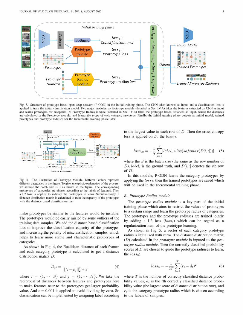
Fig. 3. Structure of prototype based open deep network (P-ODN) in the Initial training phase. The CNN takes knowns as input, and a classification loss isapplied to train the initial classification model. Two major modules: a) Prototype module (detailed in Sec. IV-A) takes the features extracted by CNN as inputand learns prototypes for categories. b) Prototype Radius module (detailed in Sec. IV-B) takes the prototype based distances as input, where the distancesare calculated in the Prototype module, and learns the scope of each category prototype. Finally, the Initial training phase outputs an initial model, trainedprototypes and prototype radiuses for the Incremental training phase later.

Fig. 4. The illustration of Prototype Module. Different colors representdifferent categories in the figure. To give an explicit explanation of the process,we assume the batch size is 3 as shown in the figure. The correspondingprototypes of categories are chosen according to the labels of features. Thena L2 loss is applied to indicate the prototypes to learn. Simultaneously, adistance distribution matrix is calculated to train the capacity of the prototypeswith the distance based classification loss.

make prototypes be similar to the features would be instable.The prototypes would be easily misled by some outliers of thetraining data samples. We add the distance based classificationloss to improve the classification capacity of the prototypesand increasing the penalty of misclassification samples, whichhelps to learn more stable and characteristic prototypes ofcategories.

As shown in Fig. 4, the Euclidean distance of each featureand each category prototype is calculated to get a distancedistribution matrix D:

Dij =1

||fi − pj ||22 + ε(4)

where i = {1, · · · , S} and j = {1, · · · , N}. We take thereciprocal of distances between features and prototypes hereto make features near to the prototypes get larger probabilityvalue. And ε = 0.001 is applied to avoid dividing by zero. Soclassification can be implemented by assigning label according

to the largest value in each row of D. Then the cross entropyloss is applied on D, the loss22:

loss22 = − 1

S

S∑i=1

[labeli ∗ log(softmax(D[i, :]))] (5)

where the S is the batch size (the same as the row number ofD), labeli is the ground truth, and D[i, :] denotes the ith rowof D.

In this module, P-ODN learns the category prototypes byapplying the loss2, then the trained prototypes are saved whichwill be used in the Incremental training phase.

B. Prototype Radius module

The prototype radius module is a key part of the initialtraining phase which aims to restrict the values of prototypesto a certain range and learn the prototype radius of categories.The prototypes and the prototype radiuses are trained jointlyby adding a L2 loss (loss3) which can be regard as aregularization item of the prototype learning.

As shown in Fig. 5, a vector of each category prototyperadius is initialized with zeros. The distance distribution matrix(D) calculated in the prototype module is inputed to the pro-totype radius module. Then the correctly classified probabilityscores of D are chosen to guide the prototype radiuses to learn,the loss3:

loss3 = − 1

2T

T∑t=1

(rt − dt)2 (6)

where T is the number of correctly classified distance proba-bility values, dt is the tth correctly classified distance proba-bility value (the largest score of distance distribution row), andrt is the category prototype radius which is chosen accordingto the labels of samples.


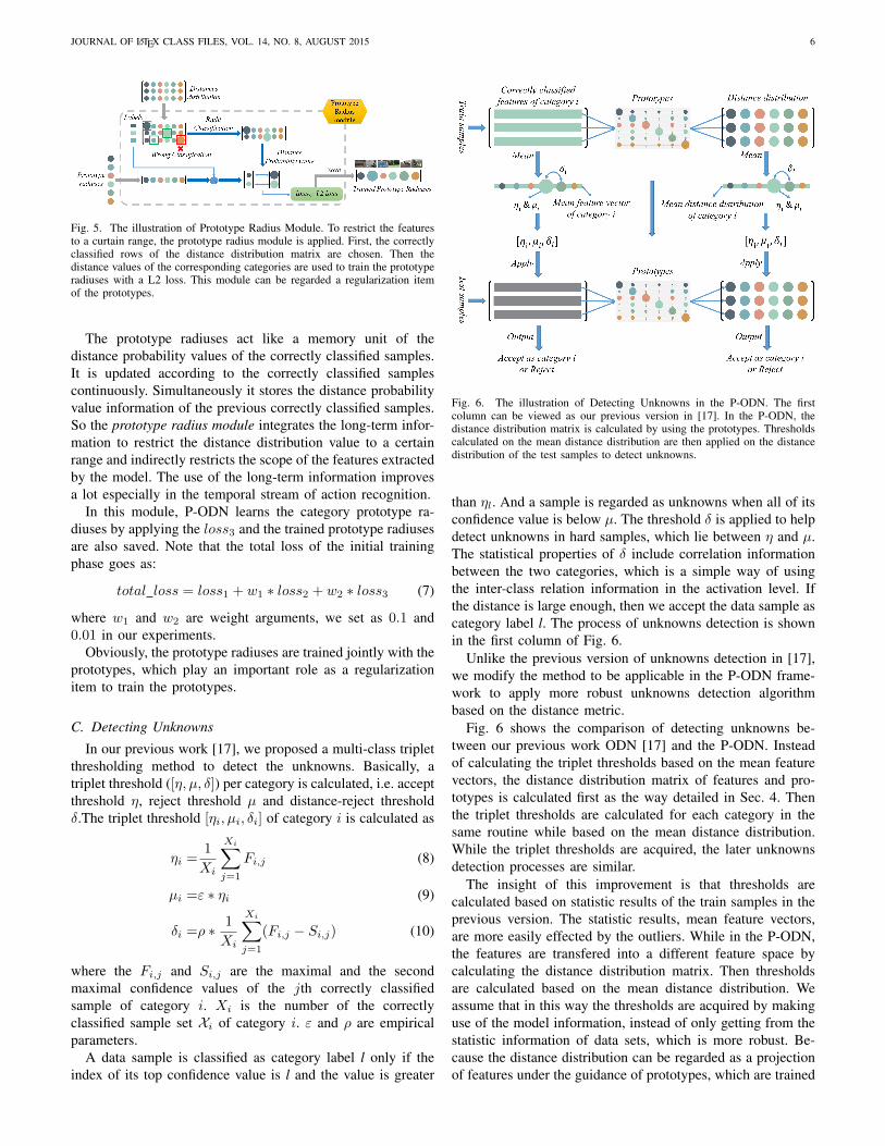
Fig. 5. The illustration of Prototype Radius Module. To restrict the featuresto a curtain range, the prototype radius module is applied. First, the correctlyclassified rows of the distance distribution matrix are chosen. Then thedistance values of the corresponding categories are used to train the prototyperadiuses with a L2 loss. This module can be regarded a regularization itemof the prototypes.

The prototype radiuses act like a memory unit of thedistance probability values of the correctly classified samples.It is updated according to the correctly classified samplescontinuously. Simultaneously it stores the distance probabilityvalue information of the previous correctly classified samples.So the prototype radius module integrates the long-term infor-mation to restrict the distance distribution value to a certainrange and indirectly restricts the scope of the features extractedby the model. The use of the long-term information improvesa lot especially in the temporal stream of action recognition.

In this module, P-ODN learns the category prototype ra-diuses by applying the loss3 and the trained prototype radiusesare also saved. Note that the total loss of the initial trainingphase goes as:

total loss = loss1 + w1 ∗ loss2 + w2 ∗ loss3 (7)

where w1 and w2 are weight arguments, we set as 0.1 and0.01 in our experiments.

Obviously, the prototype radiuses are trained jointly with theprototypes, which play an important role as a regularizationitem to train the prototypes.

C. Detecting Unknowns

In our previous work [17], we proposed a multi-class tripletthresholding method to detect the unknowns. Basically, atriplet threshold ([η, µ, δ]) per category is calculated, i.e. acceptthreshold η, reject threshold µ and distance-reject thresholdδ.The triplet threshold [ηi, µi, δi] of category i is calculated as

ηi =1

Xi

Xi∑j=1

Fi,j (8)

µi =ε ∗ ηi (9)

δi =ρ ∗1

Xi

Xi∑j=1

(Fi,j − Si,j) (10)

where the Fi,j and Si,j are the maximal and the secondmaximal confidence values of the jth correctly classifiedsample of category i. Xi is the number of the correctlyclassified sample set Xi of category i. ε and ρ are empiricalparameters.

A data sample is classified as category label l only if theindex of its top confidence value is l and the value is greater

Fig. 6. The illustration of Detecting Unknowns in the P-ODN. The firstcolumn can be viewed as our previous version in [17]. In the P-ODN, thedistance distribution matrix is calculated by using the prototypes. Thresholdscalculated on the mean distance distribution are then applied on the distancedistribution of the test samples to detect unknowns.

than ηl. And a sample is regarded as unknowns when all of itsconfidence value is below µ. The threshold δ is applied to helpdetect unknowns in hard samples, which lie between η and µ.The statistical properties of δ include correlation informationbetween the two categories, which is a simple way of usingthe inter-class relation information in the activation level. Ifthe distance is large enough, then we accept the data sample ascategory label l. The process of unknowns detection is shownin the first column of Fig. 6.

Unlike the previous version of unknowns detection in [17],we modify the method to be applicable in the P-ODN frame-work to apply more robust unknowns detection algorithmbased on the distance metric.

Fig. 6 shows the comparison of detecting unknowns be-tween our previous work ODN [17] and the P-ODN. Insteadof calculating the triplet thresholds based on the mean featurevectors, the distance distribution matrix of features and pro-totypes is calculated first as the way detailed in Sec. 4. Thenthe triplet thresholds are calculated for each category in thesame routine while based on the mean distance distribution.While the triplet thresholds are acquired, the later unknownsdetection processes are similar.

The insight of this improvement is that thresholds arecalculated based on statistic results of the train samples in theprevious version. The statistic results, mean feature vectors,are more easily effected by the outliers. While in the P-ODN,the features are transfered into a different feature space bycalculating the distance distribution matrix. Then thresholdsare calculated based on the mean distance distribution. Weassume that in this way the thresholds are acquired by makinguse of the model information, instead of only getting from thestatistic information of data sets, which is more robust. Be-cause the distance distribution can be regarded as a projectionof features under the guidance of prototypes, which are trained


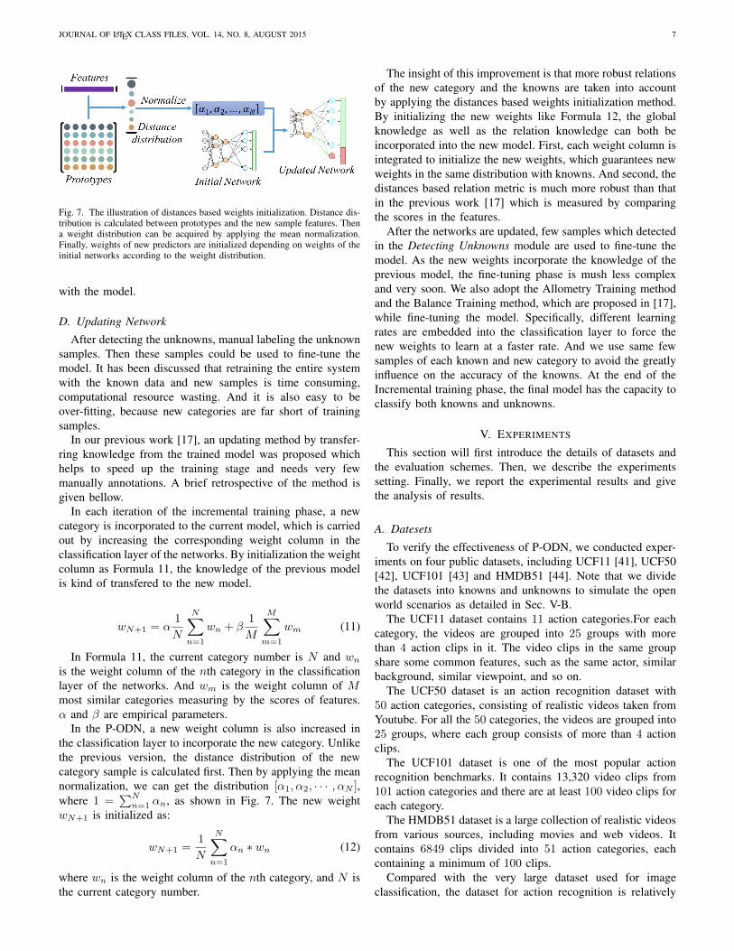
Fig. 7. The illustration of distances based weights initialization. Distance dis-tribution is calculated between prototypes and the new sample features. Thena weight distribution can be acquired by applying the mean normalization.Finally, weights of new predictors are initialized depending on weights of theinitial networks according to the weight distribution.

with the model.

D. Updating Network

After detecting the unknowns, manual labeling the unknownsamples. Then these samples could be used to fine-tune themodel. It has been discussed that retraining the entire systemwith the known data and new samples is time consuming,computational resource wasting. And it is also easy to beover-fitting, because new categories are far short of trainingsamples.

In our previous work [17], an updating method by transfer-ring knowledge from the trained model was proposed whichhelps to speed up the training stage and needs very fewmanually annotations. A brief retrospective of the method isgiven bellow.

In each iteration of the incremental training phase, a newcategory is incorporated to the current model, which is carriedout by increasing the corresponding weight column in theclassification layer of the networks. By initialization the weightcolumn as Formula 11, the knowledge of the previous modelis kind of transfered to the new model.

wN+1 = α1

N

N∑n=1

wn + β1

M

M∑m=1

wm (11)

In Formula 11, the current category number is N and wn

is the weight column of the nth category in the classificationlayer of the networks. And wm is the weight column of Mmost similar categories measuring by the scores of features.α and β are empirical parameters.

In the P-ODN, a new weight column is also increased inthe classification layer to incorporate the new category. Unlikethe previous version, the distance distribution of the newcategory sample is calculated first. Then by applying the meannormalization, we can get the distribution [α1, α2, · · · , αN ],where 1 =

∑Nn=1 αn, as shown in Fig. 7. The new weight

wN+1 is initialized as:

wN+1 =1

N

N∑n=1

αn ∗ wn (12)

where wn is the weight column of the nth category, and N isthe current category number.

The insight of this improvement is that more robust relationsof the new category and the knowns are taken into accountby applying the distances based weights initialization method.By initializing the new weights like Formula 12, the globalknowledge as well as the relation knowledge can both beincorporated into the new model. First, each weight column isintegrated to initialize the new weights, which guarantees newweights in the same distribution with knowns. And second, thedistances based relation metric is much more robust than thatin the previous work [17] which is measured by comparingthe scores in the features.

After the networks are updated, few samples which detectedin the Detecting Unknowns module are used to fine-tune themodel. As the new weights incorporate the knowledge of theprevious model, the fine-tuning phase is mush less complexand very soon. We also adopt the Allometry Training methodand the Balance Training method, which are proposed in [17],while fine-tuning the model. Specifically, different learningrates are embedded into the classification layer to force thenew weights to learn at a faster rate. And we use same fewsamples of each known and new category to avoid the greatlyinfluence on the accuracy of the knowns. At the end of theIncremental training phase, the final model has the capacity toclassify both knowns and unknowns.

V. EXPERIMENTS

This section will first introduce the details of datasets andthe evaluation schemes. Then, we describe the experimentssetting. Finally, we report the experimental results and givethe analysis of results.

A. Datesets

To verify the effectiveness of P-ODN, we conducted exper-iments on four public datasets, including UCF11 [41], UCF50[42], UCF101 [43] and HMDB51 [44]. Note that we dividethe datasets into knowns and unknowns to simulate the openworld scenarios as detailed in Sec. V-B.

The UCF11 dataset contains 11 action categories.For eachcategory, the videos are grouped into 25 groups with morethan 4 action clips in it. The video clips in the same groupshare some common features, such as the same actor, similarbackground, similar viewpoint, and so on.

The UCF50 dataset is an action recognition dataset with50 action categories, consisting of realistic videos taken fromYoutube. For all the 50 categories, the videos are grouped into25 groups, where each group consists of more than 4 actionclips.

The UCF101 dataset is one of the most popular actionrecognition benchmarks. It contains 13,320 video clips from101 action categories and there are at least 100 video clips foreach category.

The HMDB51 dataset is a large collection of realistic videosfrom various sources, including movies and web videos. Itcontains 6849 clips divided into 51 action categories, eachcontaining a minimum of 100 clips.

Compared with the very large dataset used for imageclassification, the dataset for action recognition is relatively


TABLE ISAMPLE NUMBER OF MANUALLY ANNOTATED UNKNOWNS NEEDED TO

INCREASE A CATEGORY ON AVERAGE.

sample number UCF11 UCF50 UCF101 HMDB51ODN 7 5.8 5.39 5.57

P-ODN 7 5.4 5.2 5

small. Therefor we pre-trained our model on the ImageNetdataset [34].

B. Experiments setting

To simulate the open world scenarios, we choose nearlyhalf categories of each data set as knowns and the otherhalf as unknowns, i.e. 6 categories of UCF11 as knownswhile the other 5 as unknowns, 25 categories of UCF50 asknowns while the other 25 as unknowns, 50 categories ofUCF101 as knowns while the other 51 as unknowns, and25 categories of HMDB51 as knowns while the other 26 asunknowns. Then the training set of each dataset is dividedinto two subsets according to knowns and unknowns. Thesubset which contains knowns is the initial training set. Asmall subset is chosen from both the knowns and unknowns,which we guarantee that each category has at least 10 samples,to form the incremental training set. Note that we use muchless training samples and removing half labels of the trainingset to simulate the open world scenarios.

After initializing from the pre-trained ImageNet model forspatial and temporal streams, we conduct the initial trainingphase to train prototypes, prototype radiuses of categories, andthe initial model jointly. Note that both the spatial stream andthe temporal stream train their own prototypes and prototyperadiuses respectively. After prototypes and prototype radiusesfor the two streams are trained, then triplet thresholds ofboth spatial and temporal streams are calculated on the initialtraining set based on the prototypes.

During the incremental training phase, we keep the sameexperiment setting as our previous work [17] to give a con-vincing comparison. Basically, we update the networks whenthe number of any labeled new category goes to 5, then thiscategory is incorporated into the current model.

The experiments show that we use 53 iterations (on average)to increase 51 new categories while using dataset UCF101 (27iterations for UCF50 to increase 25, 7 iterations for UCF11 toincrease 5 and 26 for HMDB51 to increase 26 new categories).So, on average, UCF101 needs to label 5.2 (53 × 5 ÷ 51 =5.2) samples (5.4 samples for UCF50, 7 samples for UCF11and 5 samples for HMDB51) for each unknown categories. Amore explict comparison is shown in the Table I between ourprevious ODN [17] and P-ODN, it is obvious that we use thesame number of labeled unknown samples in the P-ODN oreven less.

However, for closed set recognition, using UCF101 as anexample, the training list of UCF101 split1 has 9537 datasamples of 101 categories. On average, each category, half ofthe categories corresponding to the known categories and halfto the unknown categories, needs 94.4 (9537 ÷ 101 = 94.4)

Fig. 8. Heat map of mean features and prototypes of knowns. Prototypes havemuch stronger response on the correctly classified values, for the diagonalline is much brighter while the upper and lower triangular matrices are muchdarker.

Fig. 9. T-SNE visualization of mean features and prototypes. Each colorednumber represents a mean feature or a prototype of a certain category. The leftvisualization of the mean features has more confusion categories which theinter-class distances are really short, while the prototypes can better handlethe confusion categories as shown in the right sub-figure.

annotated samples. It is obvious that we use much less samplesof unknowns in the open set setting.

We also conduct the closed set recognition experiments asour baseline using the same sample size as the open set setting.The results of experiments in closed set setting are muchless than those of our P-ODN while both using insufficientunknown samples(detailed in Sec. V-D). So, P-ODN needsmuch fewer human annotations then the closed set recognition,and can achieve better performance. Worth to mention that,P-ODN suits the real world scenarios, while the closed setrecognition can not handle these tasks.

We use the Tensorflow toolbox [45]. And we give the resultson Inception-resnet-v2. The network weights are trained usingthe mini-batch stochastic gradient descent with momentum (setto 0.9). We resize all input images to 340× 256, and then usethe fixed- crop strategy [46] to crop a 299× 299 region fromimages or their horizontal flip.

C. Exploration experiments

Benefits from prototypes. To illustrate the improvement ofprototypes, we firstly conduct an exploration experiments onUCF101 with GoogLeNet [27].

We visualize the heat map of the mean features and pro-totypes of the knowns, as shown in Fig. 8. We can seethat prototypes have much stronger response on the correctly


(a) UCF11 (b) UCF50

(c) UCF101 (d) HMDB51

Fig. 10. Comparison of baseline method, ODN [17], P-ODN and P-ODN with radius on category accuracy of UCF11, UCF50, UCF101 and HMDB51 in realworld scenarios. Each sub-figure is corresponding to a data set, taking the sub-figure 10a as an example. The light gray bar denotes the accuracy of knownsof baseline, while the dull gray denotes the accuracy of unknowns of baseline. The light blue line denotes the accuracy of knowns of ODN, while the darkblue denotes the accuracy of unknowns of ODN. And so on, the light green denotes the knowns of P-ODN and dark green denotes the unknowns of P-ODN.The light red and the dark red denote the knowns and unknowns of P-ODN with radius respectively.

classified values, for the diagonal line is much brighter whilethe upper and lower triangular matrices are much darker.

As shown in Fig. 9, we reduce dimensions of the meanfeatures and the prototypes, and visualize them by applying t-SNE. In the figure, each colored number represents one meanfeature of a certain category or one prototype of a certaincategory. The left visualization of the mean features has moreconfusion categories which the inter-class distances are reallyshort, while the prototypes can better handle the confusioncategories as shown in the right sub-figure.

The comparison shows that the prototypes are more suitablefor representing category centers. Because the prototypes havestronger response on the collected classified values and longerinter-class distances. The two advantages help to complementmore robust unknowns detection and guide much better fea-tures training.

D. Evaluation of detecting unknowns

In this subsection, we aim to evaluate the unknowns detec-tion performance of our P-ODN on UCF11, UCF50, UCF101

TABLE IIUNKNOWNS DETECTION RESULTS OF P-ODN.

F-score UCF11 UCF50 UCF101 HMDB51OSDN [13] 82.59% 75.34% 72.1% 50.31%ODN [17] 87.39% 74.91% 73.35% 63.70%

P-ODN 89.12% 80.14% 75.45% 66.79%P-ODN + radius 89.50% 82.15% 76.2% 67.36%

and HMDB51. As mentioned before, we conduct this evalu-ation at the end of initial training phase as Evaluation phase1. The experimental results are summarized in Table II. Thefirst row of the results is the performance of OSDN proposedin [13], we conduct the method on the action recognitiontask. The second row is the performance of our previouswork [17]. And the third row is the performance of P-ODNwith prototype module only, the last row is P-ODN with bothprototype module and prototype radius module. We can seeP-ODN with both prototype module and the prototype radiusmodule improves the ODN by 2.11% on UCF11, 7.24% onUCF50, 2.85% on UCF101 and 3.66% on HMDB51.


TABLE IIIRECOGNITION RESULTS OF P-ODN.

TOP1 Acc. UCF11 UCF50 UCF101 HMDB51baseline 85.1% 84.95% 72.01% 44.58%

ODN [17] 94.91% 93.73% 76.07% 46.01%P-ODN 94.9% 95.16% 77.21% 47.84%

P-ODN + radius 95.31% 96.15% 78.64% 49.09%

As mentioned in Sec. IV-C and shown in Sec. V-C, un-knowns detection based on the prototypes are more robust.First the prototypes are more discriminable than mean features.Second the prototypes can guide the features to be trainedbetter, which helps to improve the intra-class compactness andinter-class distance of the feature representation. We also learnthe triplet thresholds based on the prototypes which wouldcontain the knowledge of the model itself. Then the muchdiscriminable features and the model based triplet thresholdsboth lead to a great improvement on the performance ofunknowns detection.

E. Evaluation of classification on both knowns and unknowns

In this subsection, we aim to evaluate the classificationperformance of our P-ODN on UCF11, UCF50, UCF101 andHMDB51. We conduct this evaluation at the end of incremen-tal training phase as Evaluation phase 2, the final classificationaccuracy of both knowns and unknowns is viewed as the mostimportant performance indicator of open set recognition tasks.The experimental results are summarized in Table III. First, wecarry out the closed set recognition experiments while usingthe same quantity of samples as those of our open set setting.Under the closed set setting, all training samples should havelabels, so we provide labels of both knowns and unknowns.The result is shown in the first row as our baseline. The restof Table III are results under the open set setting as detailedin Sec. V-B. The second row is the result in our previouswork [17], and we add the experiment on UCF11 here, sincewe did not use UCF11 in the previous work. The last rowis P-ODN with both prototype module and prototype radiusmodule, which achieves the best performance. We can see P-ODN finally improves the ODN by 0.3% on UCF11, 2.42%on UCF50, 2.57% on UCF101 and 3.08% on HMDB51. Andfurthermore, P-ODN finally improves the baseline by 10.21%on UCF11, 11.2% on UCF50, 6.63% on UCF101 and 4.51%on HMDB51.

A more explicit illustration can be see in Fig. 10. Each sub-figure is corresponding to a data set, UCF11, UCF50, UCF101and HMDB51. Take the sub-figure 10a as an example, wecompare the accuracy of both knowns and unknowns onUCF11 with four methods, which are baseline, ODN [17],P-ODN and P-ODN with radius (P-ODN with both prototypemodule and the prototype radius module). The light gray bardenotes the accuracy of knowns of baseline, while the dullgray denotes the accuracy of unknowns of baseline. The lightblue line denotes the accuracy of knowns of ODN, while thedark blue denotes the accuracy of unknowns of ODN. And soon, the light green denotes the knowns of P-ODN and darkgreen denotes the unknowns of P-ODN. The light red and the

dark red denote the knowns and unknowns of P-ODN withradius respectively.

We can see that while using the baseline method, theknowns which are trained with abundant data samples canachieve a much better performance than the unknowns whichare trained with insufficient data samples with labels. Ourmethods can improve greatly on unknowns while using in-sufficient samples. Though, the performance on the knownsmay decrease slightly, since the fine-tuning phase incorporatesnew data continuously. In Fig. 10, we can see P-ODN withradius is generally above the other methods, which achievesthe best performance. Note that, different from the baselinemethod which is provided with all labels beforehand, the otherthree methods should detect the unknowns first, then manuallabeling the unknowns. Therefore, open set recognition is morerealistic then the closed set setting.

VI. CONCLUSION

This paper proposed a prototype based Open Deep Network(P-ODN) for open set recognition. We introduce prototypelearning into open set recognition tasks by training prototypesof categories and prototype radiuses with a prototype moduleand a prototype radius module. Then a distance metric methodis applied to detect unknowns, which is based on the proto-types and more robust. In the incremental training phase, adistances based weights initialization method is employed tofast acquire the knowledge of model and speed up the fine-tuning process. Experimental results show that, our P-ODNcan effectively detect and recognize new categories with littlehuman intervention and achieve state-of-the-art performanceon UCF11, UCF50, UCF101 and HMDB51 datasets.

In this paper, we have proved the importance of more dis-criminable centers (or prototypes) on the open set recognitiontasks. More characteristic features which have larger marginamong categories will further improve the performance ofunknowns detection. In addition, method [47] utilizes GANto generate unknown samples and uses them to train theneural networks also has potential to improve the recognitionperformance of unknowns. In the future work, we will conductmore experiments as mentioned above to further improve theperformance of open set recognition.

REFERENCES

[1] A. Krizhevsky, I. Sutskever, and G. E. Hinton, “Imagenet classificationwith deep convolutional neural networks,” in Advances in neural infor-mation processing systems, 2012, pp. 1097–1105.

[2] L. Wang, Y. Xiong, Z. Wang, Y. Qiao, D. Lin, X. Tang, and L. Van Gool,“Temporal segment networks: Towards good practices for deep actionrecognition,” in European Conference on Computer Vision. Springer,2016, pp. 20–36.

[3] Y. Shi, Y. Tian, Y. Wang, W. Zeng, and T. Huang, “Learning long-termdependencies for action recognition with a biologically-inspired deepnetwork,” in Proceedings of the International Conference on ComputerVision, 2017, pp. 716–725.

[4] A. Tveit and M. L. Hetland, “Multicategory incremental proximalsupport vector classifiers,” in International Conference on Knowledge-Based and Intelligent Information and Engineering Systems. Springer,2003, pp. 386–392.

[5] G. Cauwenberghs and T. Poggio, “Incremental and decremental supportvector machine learning,” in Advances in neural information processingsystems, 2001, pp. 409–415.


[6] K. Crammer, O. Dekel, J. Keshet, S. Shalev-Shwartz, and Y. Singer,“Online passive-aggressive algorithms,” Journal of Machine LearningResearch, vol. 7, no. Mar, pp. 551–585, 2006.

[7] T. Yeh and T. Darrell, “Dynamic visual category learning,” 2008.[8] M. Herbster, “Learning additive models online with fast evaluating ker-

nels,” in International Conference on Computational Learning Theory.Springer, 2001, pp. 444–460.

[9] T. Mensink, J. Verbeek, F. Perronnin, and G. Csurka, “Metric learning forlarge scale image classification: Generalizing to new classes at near-zerocost,” in Computer Vision–ECCV 2012. Springer, 2012, pp. 488–501.

[10] I. Kuzborskij, F. Orabona, and B. Caputo, “From n to n+ 1: Multiclasstransfer incremental learning,” in Proceedings of the IEEE Conferenceon Computer Vision and Pattern Recognition, 2013, pp. 3358–3365.

[11] A. S. T. E. B. W. J. Scheirer, A. Rocha, “Towards open set recognition,”in IEEE, 2013.

[12] W. J. Scheirer, L. P. Jain, and T. E. Boult, “Probability models for openset recognition,” IEEE transactions on pattern analysis and machineintelligence, vol. 36, no. 11, pp. 2317–2324, 2014.

[13] A. Bendale and T. E. Boult, “Towards open set deep networks,” inProceedings of the IEEE conference on computer vision and patternrecognition, 2016, pp. 1563–1572.

[14] A. Bendale and T. Boult, “Towards open world recognition,” in Pro-ceedings of the IEEE Conference on Computer Vision and PatternRecognition, 2015, pp. 1893–1902.

[15] M. Ristin, M. Guillaumin, J. Gall, and L. Van Gool, “Incremental learn-ing of ncm forests for large-scale image classification,” in Proceedingsof the IEEE conference on computer vision and pattern recognition,2014, pp. 3654–3661.

[16] H.-M. Yang, X.-Y. Zhang, F. Yin, and C.-L. Liu, “Robust classificationwith convolutional prototype learning,” in Proceedings of the IEEEConference on Computer Vision and Pattern Recognition, 2018, pp.3474–3482.

[17] Y. Shu, Y. Shi, Y. Wang, Y. Zou, Q. Yuan, and Y. Tian, “Odn:Opening the deep network for open-set action recognition,” in 2018IEEE International Conference on Multimedia and Expo (ICME). IEEE,2018, pp. 1–6.

[18] A. Pronobis, L. Jie, and B. Caputo, “The more you learn, the less youstore: Memory-controlled incremental svm for visual place recognition,”Image and Vision Computing, vol. 28, no. 7, pp. 1080–1097, 2010.

[19] N. A. Syed, S. Huan, L. Kah, and K. Sung, “Incremental learning withsupport vector machines,” 1999.

[20] G. Fung and O. L. Mangasarian, “Incremental support vector machineclassification,” in Proceedings of the 2002 SIAM International Confer-ence on Data Mining. SIAM, 2002, pp. 247–260.

[21] Z. Wang, K. Crammer, and S. Vucetic, “Multi-class pegasos on a bud-get,” in Proceedings of the 27th International Conference on MachineLearning (ICML-10). Citeseer, 2010, pp. 1143–1150.

[22] S. Shalev-Shwartz, Y. Singer, N. Srebro, and A. Cotter, “Pegasos: Primalestimated sub-gradient solver for svm,” Mathematical programming, vol.127, no. 1, pp. 3–30, 2011.

[23] W. J. Scheirer, A. Rocha, R. J. Micheals, and T. E. Boult, “Meta-recognition: The theory and practice of recognition score analysis,” IEEEtransactions on pattern analysis and machine intelligence, vol. 33, no. 8,pp. 1689–1695, 2011.

[24] P. Zhang, J. Wang, A. Farhadi, M. Hebert, and D. Parikh, “Predictingfailures of vision systems,” in Proceedings of the IEEE Conference onComputer Vision and Pattern Recognition, 2014, pp. 3566–3573.

[25] K. He, X. Zhang, S. Ren, and J. Sun, “Deep residual learning for imagerecognition,” in Proceedings of the IEEE conference on computer visionand pattern recognition, 2016, pp. 770–778.

[26] I. Sutskever, O. Vinyals, and Q. V. Le, “Sequence to sequence learningwith neural networks,” in Advances in neural information processingsystems, 2014, pp. 3104–3112.

[27] C. Szegedy, W. Liu, Y. Jia, P. Sermanet, S. Reed, D. Anguelov, D. Erhan,V. Vanhoucke, and A. Rabinovich, “Going deeper with convolutions,”in Proceedings of the IEEE conference on computer vision and patternrecognition, 2015, pp. 1–9.

[28] K. He, X. Zhang, S. Ren, and J. Sun, “Delving deep into rectifiers:Surpassing human-level performance on imagenet classification,” inProceedings of the IEEE international conference on computer vision,2015, pp. 1026–1034.

[29] N. Dalal and B. Triggs, “Histograms of oriented gradients for humandetection,” in Computer Vision and Pattern Recognition, 2005. CVPR2005. IEEE Computer Society Conference on, vol. 1. IEEE, 2005, pp.886–893.

[30] N. Dalal, B. Triggs, and C. Schmid, “Human detection using orientedhistograms of flow and appearance,” in European conference on com-puter vision. Springer, 2006, pp. 428–441.

[31] Y. Shi, W. Zeng, T. Huang, Y. Wang et al., “Learning deep trajectory de-scriptor for action recognition in videos using deep neural networks,” in2015 IEEE International Conference on Multimedia and Expo (ICME).IEEE, 2015, pp. 1–6.

[32] S. Zha, F. Luisier, W. Andrews, N. Srivastava, and R. Salakhutdinov,“Exploiting image-trained cnn architectures for unconstrained videoclassification,” arXiv preprint arXiv:1503.04144, 2015.

[33] K. Simonyan and A. Zisserman, “Two-stream convolutional networksfor action recognition in videos,” in Advances in neural informationprocessing systems, 2014, pp. 568–576.

[34] J. Deng, W. Dong, R. Socher, L.-J. Li, K. Li, and L. Fei-Fei, “Imagenet:A large-scale hierarchical image database,” in Computer Vision andPattern Recognition, 2009. CVPR 2009. IEEE Conference on. Ieee,2009, pp. 248–255.

[35] Z. Zhou, F. Shi, and W. Wu, “Learning spatial and temporal extents ofhuman actions for action detection,” IEEE Transactions on multimedia,vol. 17, no. 4, pp. 512–525, 2015.

[36] M. Hasan and A. K. Roy-Chowdhury, “A continuous learning frame-work for activity recognition using deep hybrid feature models,” IEEETransactions on Multimedia, vol. 17, no. 11, pp. 1909–1922, 2015.

[37] L. Pang, S. Zhu, and C.-W. Ngo, “Deep multimodal learning for affectiveanalysis and retrieval,” IEEE Transactions on Multimedia, vol. 17,no. 11, pp. 2008–2020, 2015.

[38] K. Simonyan and A. Zisserman, “Very deep convolutional networks forlarge-scale image recognition,” arXiv preprint arXiv:1409.1556, 2014.

[39] S. Ioffe and C. Szegedy, “Batch normalization: Accelerating deepnetwork training by reducing internal covariate shift,” arXiv preprintarXiv:1502.03167, 2015.

[40] Y. Shi, Y. Tian, Y. Wang, and T. Huang, “Sequential deep trajectorydescriptor for action recognition with three-stream cnn,” IEEE Transac-tions on Multimedia, vol. 19, no. 7, pp. 1510–1520, 2017.

[41] J. Liu, J. Luo, and M. Shah, “Recognizing realistic actions from videosin the wild,” in Computer vision and pattern recognition, 2009. CVPR2009. IEEE conference on. IEEE, 2009, pp. 1996–2003.

[42] K. K. Reddy and M. Shah, “Recognizing 50 human action categoriesof web videos,” Machine Vision and Applications, vol. 24, no. 5, pp.971–981, 2013.

[43] K. Soomro, A. R. Zamir, and M. Shah, “Ucf101: A dataset of 101 humanactions classes from videos in the wild,” arXiv preprint arXiv:1212.0402,2012.

[44] H. Kuehne, H. Jhuang, E. Garrote, T. Poggio, and T. Serre, “Hmdb:a large video database for human motion recognition,” in ComputerVision (ICCV), 2011 IEEE International Conference on. IEEE, 2011,pp. 2556–2563.

[45] M. Abadi, P. Barham, J. Chen, Z. Chen, A. Davis, J. Dean, M. Devin,S. Ghemawat, G. Irving, M. Isard et al., “Tensorflow: a system for large-scale machine learning.” in OSDI, vol. 16, 2016, pp. 265–283.

[46] L. Wang, Y. Xiong, Z. Wang, and Y. Qiao, “Towards good practicesfor very deep two-stream convnets,” arXiv preprint arXiv:1507.02159,2015.

[47] Z. Ge, S. Demyanov, Z. Chen, and R. Garnavi, “Generative openmaxfor multi-class open set classification,” arXiv preprint arXiv:1707.07418,2017.

Yu Shu received the B.S. degree in computer sci-ence from Peking University, Beijing, China, in2017. He is currently working toward the master’sdegree at the School of Academy for AdvancedInterdisciplinary Studies, Peking University, Beijing,China. His research interests include machine learn-ing, open set recognition, action recognition andcomputer vision.


Yemin Shi received the B.S. degree from PekingUniversity, Beijing, China, in 2014. He is currentlyworking toward the Ph.D. degree at the Schoolof Electrical Engineering and Computer Science,Peking University, Beijing, China. His research in-terests include machine learning, anomaly detection,action recognition and computer vision.

Yaowei Wang, Ph.D., is currently an assistant pro-fessor at the Department of Electronics Engineer-ing, Beijing Institute of Technology. He is alsoa guest assistant professor at the National Engi-neering Laboratory for Video Technology (NELVT),Peking University, China. He received Ph.D. degreeon Computer Science from Graduate University ofChinese Academy of Sciences in 2005. His researchinterests include machine learning, multimedia con-tent analysis and understanding. He is the author orcoauthor of over 40 refereed journals and conference

papers. His team was ranked as one of the best performers in the TRECVIDCCD/SED tasks from 2009 to 2012 and PETS 2012. He is a member of IEEEand CIE.

Tiejun Huang, Ph.D, is a Professor with the Schoolof Electronic Engineering and Computer Science,Head of Department of Computer Science, PekingUniversity. His research areas include video codingand image understanding, especially neural codinginspired information coding theory in recent years.He received the Ph.D. degree in pattern recognitionand intelligent system from the Huazhong (CentralChina) University of Science and Technology in1998, and the masters and bachelors degrees incomputer science from the Wuhan University of

Technology in 1995 and 1992, respectively. Professor Huang received theNational Science Fund for Distinguished Young Scholars of China in 2014,and was awarded the Distinguished Professor of the Chang Jiang ScholarsProgram by the Ministry of Education in 2015. He is a member of theBoard of the Chinese Institute of Electronics and the Advisory Board of IEEEComputing Now.

Yonghong Tian is currently a full professor withthe National Engineering Laboratory for Video Tech-nology and the Cooperative Medianet InnovationCenter, School of Electronics Engineering and Com-puter Science, Peking University, Beijing, China.He received the Ph.D. degree from the Institute ofComputing Technology, Chinese Academy of Sci-ences, China, in 2005. His research interests includemachine learning, computer vision, and multimediabig data. He is the author or coauthor of over 140technical articles in refereed journals and confer-

ences, and has owned more than 35 patents. Dr. Tian is currently an AssociateEditor of IEEE Transactions on Multimedia, and International Journal ofMultimedia Data Engineering and Management (IJMDEM). He has servedas the Technical Program Co-chair of IEEE ICME 2015, IEEE BigMM2015 and IEEE ISM 2015, the organizing committee member of more thanten conferences such as ACM Multimedia 2009, IEEE MMSP 2011, IEEEISCAS 2013, IEEE ISM 2016, and the PC member of several top conferencessuch as CVPR, KDD, AAAI and ECCV. He was the recipient of severalnational and ministerial prizes in China, and obtained the 2015 EURASIPBest Paper Award for the EURASIP Journal on Image and Video Processing.His team was also ranked as one of the best performers in the TRECVIDCCD/SED tasks from 2009 to 2012, PETS 2012 and the WikipediaMM taskin ImageCLEF 2008. He is a senior member of IEEE and CIE, a member ofACM and CCF.

JOURNAL OF LA P-ODN: Prototype based Open Deep Network for ...

Documents

Transcript of JOURNAL OF LA P-ODN: Prototype based Open Deep Network for ...