JOURNAL OF LA An accurate boundary value problem solver ... · An accurate boundary value problem...

JOURNAL OF LATEX CLASS FILES, VOL. 6, NO. 1, JANUARY 2007 1

An accurate boundary value problem solver appliedto scattering from cylinders with corners

Johan Helsing and Anders Karlsson

Abstract—In this paper we consider the classic problem ofscattering of waves from perfectly conducting cylinders withpiecewise smooth boundaries. The scattering problems are for-mulated as integral equations and solved using a Nystromscheme, where the corners of the cylinders are efficiently handledby a method referred to as Recursively Compressed InversePreconditioning (RCIP). This method has been very successfulin treating static problems in non-smooth domains and thepresent paper shows that it works equally well for the Helmholtzequation. In the numerical examples we focus on scattering ofE- and H-waves from a cylinder with one corner. Even at a sizekd = 1000, where k is the wavenumber and d the diameter, thescheme produces at least 13 digits of accuracy in the electric andmagnetic fields everywhere outside the cylinder.

Index Terms—Scattering, Helmholtz equation, integral equa-tions, Nystrom method.

I. INTRODUCTION

THE numerical simulation of scattering from cylindershas a long history in computational electromagnetics.

As early as 1881, Lord Rayleigh treated the scattering oflight from a circular dielectric cylinder [1]. He considered anincident plane E-wave, i.e., the electric field is parallel to thecylinder, and a permittivity and permeability of the cylinderthat departed only slightly from those of the surroundingmedium. This approach enabled him to find an approximatesolution that today is referred to as the Born approximationand can be viewed as spectral method solution with only onebasis function, c.f. [2, Section 8.3.4]. The theory of scatteringfrom circular cylinders and spheres, conducting or dielectric,was soon after that fully understood by using expansions of theincident and scattered waves in partial waves, c.f. [3]. Sincethen, a large number of papers have been published that solvescattering problems in electromagnetics, as well as in acousticsand elastodynamics, using different numerical techniques. Allwith the common goal of constructing faster and more accuratesolvers for ever more detailed and complex geometries in twoand three space dimensions. In particular, integral equationmethods have become very important tools. In electromag-netics such methods were made popular by the contributionsof Harrington, c.f. [4]. The mathematical foundations of thescattering problems and the integral equation formulations arediscussed in the books by Colton and Kress [5], [6].

The present paper is about scattering from piecewise smoothperfectly conducting objects. The presence of boundary sin-

J. Helsing is with the Centre for Mathematical Sciences, Lund University,Box 118, 221 00 Lund, Sweden e-mail: ([email protected]).

A. Karlsson is with Electrical and Information Technology, Lund University,Box 118, 221 00 Lund, Sweden e-mail: ([email protected]).

gularities, such as corners, tends to cause complicated asymp-totics in quantities used to represent the solution. Intensemesh refinement might be needed for resolution, but this iscostly and can easily lead to instabilities and the loss ofprecision in the computed field. In the context of integralequation solvers, regions close to the boundary are the mostproblematic. On the application side, scattering from non-smooth metal objects is of great importance in radar imagingof objects with sharp corners such as airplanes, vessels andvehicles. Sharp corners that are oriented perpendicular to theline of sight of a monostatic radar may create reflectionsthat are large enough to be detected by the radar. The two-dimensional approximations can be used for elongated objectslike wings but also in the evaluation of fields in the near zoneof smaller objects. Other important two-dimensional problemsare wave propagation in rectangular waveguides, photonicband gap structures, and substrate integrated waveguides.

The numerical solver used in this paper takes its start-ing point in a Fredholm second kind integral equation. Theintegral operators are compact away from boundary singu-larities and the unknown quantity is a layer density repre-senting the solution to the original problem. The integralequation is discretized using a Nystrom scheme and compositeGauss–Legendre quadrature. At the heart of the solver lies amethod called Recursively Compressed Inverse Precondition-ing (RCIP). This method modifies the kernels of the integraloperators so that the layer density becomes piecewise smoothand simple to resolve by polynomials. Loosely speaking onecan say that RCIP makes it possible to solve elliptic boundaryvalue problems in piecewise smooth domains as cheaply andaccurately as they can be solved in smooth domains. The RCIPmethod originated in 2008 [7] and has been extended andsuccessfully applied to electrostatic and elastostatic problemswhich, at first glance, might seem impossible. For example, theeffective conductivity of a high-contrast conducting checker-board with a million randomly placed squares in the unitcell was computed on a regular workstation with a relativeaccuracy of 10−9 [8]. In [9], a new record was established forthe three-dimensional problem of determining the capacitanceof the unit cube – 13 digits compared to the seven digits thatwere previously known.

When we now apply the RCIP method to the Helmholtzequation we do this in a two-dimensional setting. We considerscattering of time-harmonic E- and H-waves from an infinitelylong perfectly conducting cylinder. Scattering problems areharder to solve than electrostatic problems, all other thingsheld equal. Planar problems provide a good testing groundprior to a move up to three dimensions [10]. As we shall see,


the transition from Laplace’s equation to the Helmholtz equa-tion is surprisingly straightforward and the results, presentedin Section IV below, are as good as the ones obtained forelectrostatics.

Our numerical solver meets five important criteria. Thefirst criterion is that it can handle cylinders with generalshapes. In practice this means cylinders with piecewise smoothboundaries and a finite, but arbitrary, number of corners. Thesecond criterion is that it can treat frequencies ranging fromzero up to large values of kd, where k is the wavenumber andd the diameter of the object. We have found that kd = 1000 iseasy to reach and for most cylinders this frequency range over-laps the frequency band where approximate high frequencymethods, e.g. unified theory of diffraction in combination withphysical optics, can be applied with reasonable accuracy. Thethird criterion is that the method can deliver accurate results forthe scattered field everywhere outside the object. Even closeto a corner and at kd = 1000 the scattered field is calculatedwith at least 13 digits of accuracy in IEEE double precisionarithmetic (16 digit precision). The fourth criterion is that themethod enables fast solvers. In the present implementationthe solver is fast only in the sense that the cost for modifyingthe kernels of the integral operators grows linearly with thenumber of corners in the computational domain. The methodcan be made fast in toto by incorporating fast multipoletechniques [11], [12] or perhaps even fast direct solvers [13],[14], [15]. The fifth criterion is that the method is automatizedand flexible and it requires only a minimum of adjustments asoperators and geometries change.

It is beyond the scope of the present paper to review theRCIP method in its entirety. In Section III we give a briefoverview and a few details on discretization issues particularto Hankel kernels. For a more thorough exposition, we referreaders to the research papers [7], [16], [17], [18] and to anewly written tutorial [19].

There are several recent journal papers that focus on speedand accuracy for two-dimensional scattering problems incomplex geometries. In [20] scattering from two-dimensionalsmooth strips are treated using integral equations and aNystrom method. In [21] the approach of [20] is generalizedto smooth slotted cylinders. A similar problem is treated in[22]. The schemes used in these papers give accurate resultsbut they cannot, in a simple way, be generalized to non-smoothgeometries. In [14] and in [23], on the other hand, very fast andalso flexible and accurate numerical schemes are developedfor the solution of integral equations modeling scattering fromgeneral objects with both corners and multi-material junctions.These papers, however, do not address the problem of accuratenear field evaluation.

II. FORMULATION OF THE PROBLEMS

We consider in-plane waves scattered by a bounded per-fectly conducting cylinder with a piecewise smooth boundaryΓ. The region outside the object is denoted Ωex, the timedependence is e−iωt and r = (x, y). Both E-waves, oftenreferred to as TM-waves, and H-waves, often referred toas TE-waves, are treated. We decompose the electric and

magnetic fields into a sum of the incident field, denotedUinc(r), generated by a source in Ωex, and the scattered field,denoted Usca(r) in both cases.

A. E-waves

We let the electric field be parallel to the cylinder, E(r) =zU(r), and let U(r) = Uinc(r) + Usca(r). The scattered fieldUsca(r) satisfies the following exterior Dirichlet problem:

∇2Usca(r) + k2Usca(r) = 0 , r ∈ Ωex (1)Usca(r) = −Uinc(r) , r ∈ Γ (2)

lim|r|→∞

√kr

(∂

∂r− ik

)Usca(r) = 0 . (3)

We write the solution as the combined integral representa-tion [6, eq. (3.25)].

Usca(r) =∫

Γ

∂Φk(r, r′)∂νr′

ρ(r′) d`′

− ik

2

∫Γ

Φk(r, r′)ρ(r′) d`′ , r ∈ Ωex , (4)

where Φk(r, r′) =i4H

(1)0 (k|r − r′|) is the free space Green

function for the Helmholz equation in two dimensions, H(1)0 is

the Hankel function of the first kind of order zero, and d` is anelement of arc length. The index k indicates that the quantityor function depends on the wavenumber k = ω/c. Insertionof (4) into (2) gives the integral equation for the layer densityρ(r)

(I + Kk − ik

2Sk)ρ(r) = −2Uinc(r) , r ∈ Γ , (5)

where

Kkρ(r) = 2∫

Γ

∂Φk(r, r′)∂νr′

ρ(r′) d`′ (6)

Skρ(r) = 2∫

Γ

Φk(r, r′)ρ(r′) d`′ . (7)

The second term on the right hand side in (4) corresponds to

the term ik

2Sk in (5) and is added in order to ensure a unique

solution for all k. The equation (5) is often referred to as anindirect combined field integral equation (ICFIE).

B. H-waves

We let the magnetic field be parallel to the cylinder, H(r) =zU(r), and let U(r) = Uinc(r) + Usca(r). The scattered fieldUsca(r) satisfies the following exterior Neumann problem

∇2Usca(r) + k2Usca(r) = 0 , r ∈ Ωex (8)∂Usca(r)

∂νr= −∂Uinc(r)

∂νr, r ∈ Γ (9)

lim|r|→∞

√kr

(∂

∂r− ik

)Usca(r) = 0 , (10)

where∂Usca(r)

∂νris the normal derivative of Usca. There are

several ways to model this problem as an integral equation. Weuse a regularized combined field integral equation since it is


always uniquely solvable. The scattered field is then obtainedfrom the representation [24]

Usca(r) =∫

Γ

Φ(r, r′)ρ(r′) d`′

+ i∫

Γ

∂Φ(r, r′)∂νr′

Sikρ(r′) d`′ , r ∈ Ωex , (11)

which after insertion into (9) gives the integral equation

(I −K ′k − iTkSik)ρ(r) = 2

∂Uinc(r)∂νr

. (12)

Here K ′k is the adjoint to the double layer operator (6)

K ′kρ(r) = 2

∫Γ

∂Φk(r, r′)∂νr

ρ(r′) d`′ , (13)

Sik is the single layer operator (7) with k replaced by ik, and

Tkρ(r) =∂

∂νrKkρ(r) . (14)

The equation (12) is sometimes referred to as ICFIE-R [24].The hypersingular operator Tk in (14) can be expressed

as a sum of a simple operator and an operator that requiresdifferentiation with respect to arc length only [25]

Tkρ(r) = 2k2

∫Γ

Φk(r, r′)(νr · νr′)ρ(r′) d`′

+ 2dd`

∫Γ

Φk(r, r′)dρ(r′)

d`′d`′ . (15)

We may then rewrite (12) in a form more amenable todiscretization

(I+Ak−iBkSik−iCkCik)ρ(r) = 2∂Uinc(r)

∂νr, r ∈ Γ , (16)

where Ak = −K ′k and

Bkρ(r) = 2k2

∫Γ

Φk(r, r′)(νr · νr′)ρ(r) d`′ (17)

Ckρ(r) = 2dd`

∫Γ

Φk(r, r′)ρ(r′) d`′ . (18)

III. NUMERICAL SCHEME

This section briefly reviews the RCIP method, for obtainingaccurate solutions to integral equations on piecewise smoothsurfaces, with a focus on basic concepts and on some detailsparticular to the Helmholtz equation. A more complete de-scription, along with demo codes in MATLAB, can be foundin [19].

A. Basics of the RCIP method

Assume that we have an integral representation of a fieldU(r), r ∈ Ωex, in terms of a layer density ρ(r) on a piecewisesmooth boundary Γ, and that this representation leads to aFredholm second kind integral equation

(I + K) ρ(r) = g(r) , r ∈ Γ . (19)

Here I is the identity, g is a piecewise smooth right hand side,and K is some integral operator with kernel K(r, r′) on Γ

that is compact away from a finite number of corners. Let ussplit the kernel

K(r, r′) = K?(r, r′) + K(r, r′) (20)

in such a way that K?(r, r′) is zero except for when r and r′

both lie close to the same corner vertex. In this latter caseK(r, r′) is zero. The kernel split (20) corresponds to anoperator split

K = K? + K , (21)

where K is a compact operator. The variable substitution

ρ(r) = (I + K?)−1ρ(r) (22)

allows us to rewrite (19) as a right preconditioned integralequation

ρ(r) + K(I + K?)−1ρ(r) = g(r) , r ∈ Γ , (23)

where the composition K(I + K?)−1 is compact.We discretize (23) using a Nystrom scheme based on com-

posite 16-point Gauss–Legendre quadrature. The quantitiesρ, K, and g should be simple to discretize and resolveaccurately on a coarse mesh made of quadrature panels Γp

of approximately equal length. Only the inverse (I + K?)−1

needs fine local meshes for its accurate resolution. We arriveat

(Icoa + KcoaR) ρcoa = gcoa , (24)

where the block-diagonal compressed weighted inverse matrixR is given by

R = PTW (Ifin + K?

fin)−1 P . (25)

In (24) and (25) subscript “coa” indicates a grid on the coarsemesh, subscript “fin” indicates grids on fine local meshes,the prolongation matrix P performs polynomial interpolationfrom the coarse grid to fine grids and PT

W is the transposeof a weighted prolongation matrix. See [19, Section 4 and 5]for details. Once (24) is solved for ρcoa, a discrete weight-corrected version of the original layer density can be obtainedfrom

ρcoa = Rρcoa . (26)

The solution U(r) can then be recovered in most of thecomputational domain using ρcoa in a discretized version ofthe integral representation for U(r).

Note that in (24), the need for resolution in corners isnot visible. The transformed layer density ρcoa on a non-smooth Γ should be as easy to solve for as the original layerdensity ρcoa in a discretization of (19) on a smooth Γ. Allcomputational difficulties are concentrated in the matrix R.Let there be n discretization points on the local fine grid closeto a particular corner on Γ. Judging from the definition (25), itseems as if computing R should be a prohibitively expensiveand also unstable undertaking for large n. Fortunately, R canbe computed via a fast and stable recursion which relies on ahierarchy of small nested meshes. This fast recursion enablesthe computation of the diagonal block of R, that correspondsto a particular corner, at a cost only proportional to n. Actually,when very large n are needed for resolution the cost can be


further reduced with the use of Newton’s method, see [19,Section 6 and 12] for details.

The fast recursion for R can also be run backwards for thepurpose of reconstructing ρfin from ρcoa. A partial reconstruc-tion of ρfin is needed when U(r) is to be evaluated at pointsin Ωex that lie close to corner vertices, see [19, Section 9].

We remark that the integral equations (5) and (16), whichare to be solved in this paper, have a more complicatedappearance than the model equation (19). In practice this posesno problems for RCIP – just some extra work. The two integraloperators in (5) can, for programming purposes, be combinedinto a single operator. The composition of integral operatorsin (16) can be treated with an expansion technique. With thehelp of two new temporary layer densities, one can arriveat a recursion for an expanded compressed inverse matrix Rwith the same structure as (25). Once R is computed one canextract separate blocks from it and use them in a more involvedversion of (24) that still uses only a single transformed globaldensity ρcoa. See [19, Section 14 and 17] for details.

B. The discretization of Hankel kernels

High-order accurate Nystrom discretization of boundaryintegral equations associated with the Helmholtz equation is atopic that has received much attention recently. See [26] fora comparison of various 2D schemes. We now present ourpreferred scheme by showing how to discretize the operatorKk of (6) and the first operator on the right hand side of (4).The other integral operators of Section II are discretized insimilar ways.

The kernel of Kk is twice that of the first operator in (4)and can, modulo a constant of i/2, be expressed as

Kk(r, r′) = k|r − r′|H(1)1 (k|r − r′|) (r − r′) · νr′

|r − r′|2, (27)

where H(1)1 is the Hankel function of the first kind of order

one. When r ∈ Γ, it is instructive to write (27) in the form

Kk(r, r′) = f(r, r′) +2iπ

log |r − r′|< Kk(r, r′) . (28)

For a fixed r ∈ Γ, we see from (27) and a series representationof H

(1)1 that f(r, r′) and <Kk(r, r′) are smooth functions

of r′ ∈ Γ and that

limr′→r

log |r − r′|< Kk(r, r′) = 0 . (29)

Consider now the integral Ip(r) over a quadrature panel Γp

Ip(r) =∫

Γp

Kk(r, r′)ρ(r′) d`′ . (30)

Let r(t) be a parameterization of Γ. Discretizing Kk meansbeing able to evaluate (30) for all r of interest, given a set ofvalues ρ(r(tj)) on each Γp.

If r is a point away from Γp, then Kk(r, r′) is a smoothfunction of r′ ∈ Γp and Ip(r) can be evaluated to highaccuracy using 16-point Gauss–Legendre quadrature

Ip(r) ≈∑

j

Kk(r, rj)ρjsjwj , (31)

where rj = r(tj), ρj = ρ(r(tj)), sj = |dr(tj)/dt|, and tjand wj are nodes and weights on Γp.

If ri is a discretization point close to Γp or on Γp, thenKk(ri, r

′) is not a (sufficiently) smooth function of r′ ∈ Γp

and we use (28) to arrive at

Ip(ri) ≈∑

j

f(ri, rj)ρjsjwj+2iπ

∑j

<Kk(ri, rj) ρjwijL ,

(32)where wijL are 16th-order product integration weights forthe logarithmic operator which can be constructed using theanalytic method in [17, Section 2.3]. The formula (32) can berearranged into a particularly convenient form

Ip(ri) ≈∑

j

Kk(ri, rj)ρjsjwj

+2iπ

∑j

<Kk(ri, rj) ρjsjwjwcorrijL , (33)

where the weight corrections,

wcorrijL =

(wijL

sjwj− log |ri − rj |

), (34)

are cheap to compute and depend only on the relative length(in parameter) of neighboring quadrature panels and on nodesand weights on a canonical panel. The formula (31) with r =ri and (33) summarize our Nystrom discretization of Kk forr ∈ Γ.

If r is a point not on Γ but in Ωex close to Γp, we write (27)in the form

Kk(r, r′) = g(r, r′) +2iπ

log |r − r′|< Kk(r, r′)

+2iπ

(r′ − r) · νr′

|r′ − r|2. (35)

We see from (27) and a series representation of H(1)1 that

g(r, r′) and <Kk(r, r′) are smooth functions of r′. Inanalogy with (33) one can write

Ip(r) ≈∑

j

Kk(r, rj)ρ(rj)sjwj

+2iπ

∑j

<Kk(r, rj) ρ(rj)sjwjwcorrjL (r)

+2iπ

∑j

ρ(rj)(

wjC(r)−(rj − r) · νrj

|rj − r|2sjwj

), (36)

where wcorrjL (r) are weight corrections as in (34), but with ri

replaced by r, and wjC(r) are 16th-order product integrationweights for the Cauchy singular operator which can be con-structed using the analytic method in [17, Section 2.1]. Theformulas (31) and (36) are used to discretize the first operatorin (4) when producing field plots.

C. Convergence and error estimates

We have investigated the convergence properties of oursolver rather thoroughly. Solutions converge rapidly with uni-form coarse mesh refinement up to a point beyond which no


102

103

10−15

10−10

10−5

100

number of panels

aver

age

poin

twis

e er

ror

Convergence for E−wave with k=1000

numerical16th order

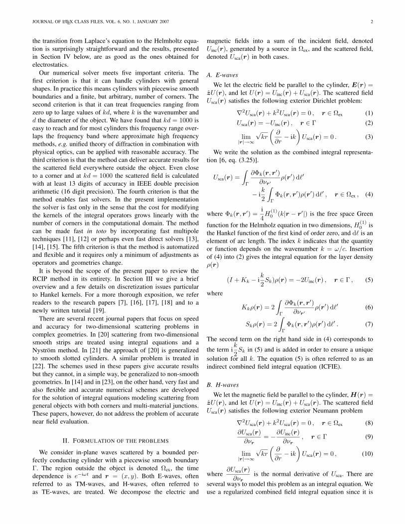
Fig. 1. The mean absolute error in <U(r) at 27,044 points exterior to Γ,as a function of the number of panels. The dashed line illustrates 16th orderconvergence. The diameter of Γ is d = 1, which means that kd = k.

further improvement occurs. Actually, beyond this point thereis a mild decay in the quality of solutions due to accumulatedroundoff error. The numerical results in the examples ofSection IV are obtained with coarse meshes that are uniformlyrefined as to provide the highest possible accuracy.

As an illustration of convergence we chose an exterior E-wave problem with a known solution. We use the non-smoothboundary Γ described by (37), below, which is also usedin all the numerical examples of Section IV. The boundaryconditions on Γ are those of an electric field generated by aline source located at r = (0.3, 0.1) inside Γ. The wavenumberis k = 1000. Evaluation points are placed on a uniform200 × 200 grid in the rectangular region x ∈ [−0.1, 1.1] andy ∈ [−0.5, 0.5]. Points inside Γ are excluded. Figure 1 showshow the mean absolute error in <U(r) at the evaluationpoints decays with uniform coarse mesh refinement. One cansee that the convergence is 16th order, consistent with theuse of 15th degree polynomial basis functions. The achievableaccuracy is close to machine precision, indicating a well-conditioned problem and a stable solver. The tutorial [19,Section 18] contains more examples in the same style.

In the plane-wave scattering examples of Section IV-A, noexact results are known. Therefore we shall estimate errors asfollows: we first compute a solution U(r) using a number ofcoarse panels on Γ deemed sufficient for resolution. We thenincrease the number of panels with 50 % and solve again.The difference between the resolved value of U(r) and theoverresolved value of U(r) is used as an indirect pointwiseerror estimate. When kd = 1000 we found that 900 panels onΓ, corresponding to 37.4 points per wavelength, gave the bestpossible resolution. Yet an indirect method to estimate the(overall) precision in the computations is by comparing thescattering cross section computed from its definition (close toΓ) with its value obtained via the optical theorem (at infinity).See, further, Section IV-B. As it turns out, the various errorestimates seem to agree well.

IV. NUMERICAL EXAMPLES

We shall now solve (5) and (16) for the unknown densityρ(r), using the method of Section III, and then evaluate thescattered fields of (4) and (11). We restrict the numericalexamples to scattering from an infinite straight cylinder withboundary Γ described by

r(t) = sin(πt) (cos((t− 0.5)π/2), sin((t− 0.5)π/2)) ,

t ∈ [0, 1] , (37)

and to the incident plane wave Uinc(r) = eiky for both E-waves and H-waves. The object parameterized in (37) hasa corner with opening angle θ = π/2 at r = (0, 0) and adiameter d = 1, in arbitrary length units, so that kd = k.The examples cover sizes from kd = 1 up to kd = 1000. Wehave seen that at kd = 1000 the frequency is high enoughsuch that the uniform theory of diffraction theory can beapplied. All numerical examples are executed in MATLABon a workstation equipped with an IntelXeon E5430 CPU at2.66 GHz and 32 GB of memory.

A. Near field

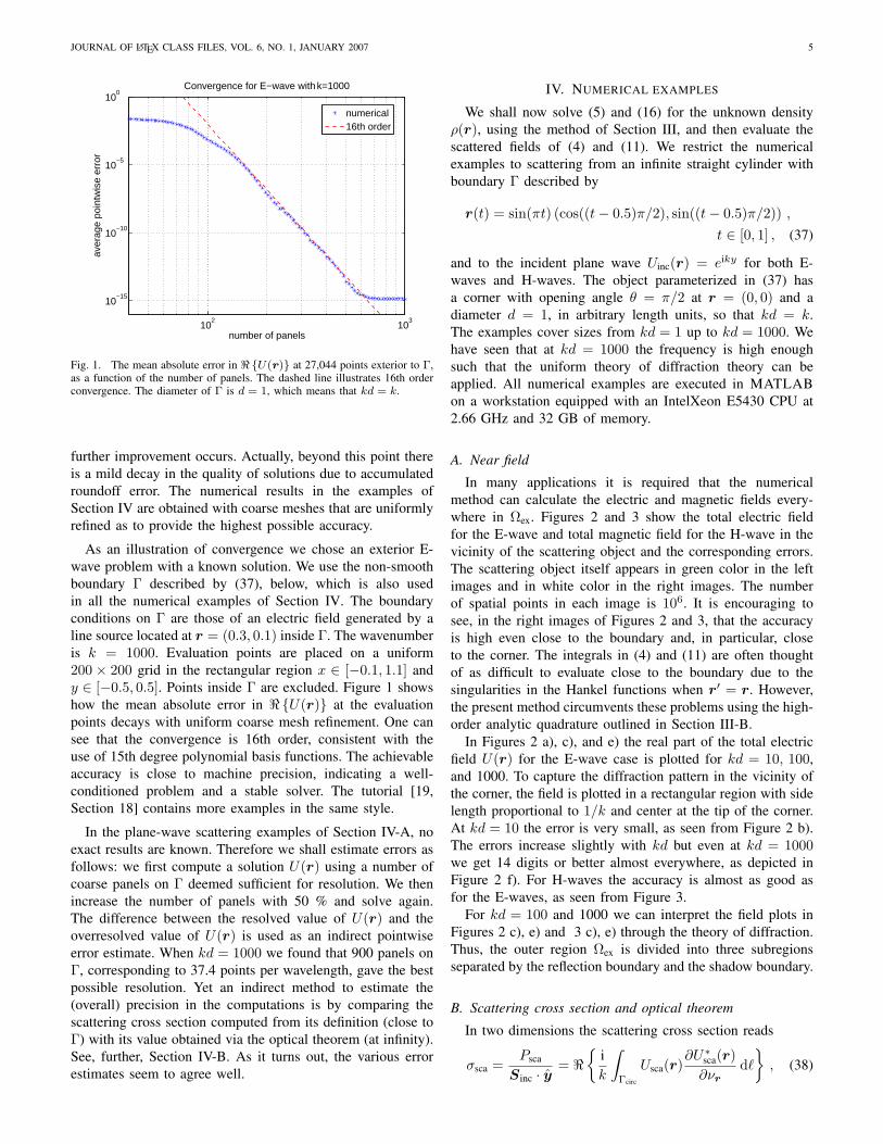
In many applications it is required that the numericalmethod can calculate the electric and magnetic fields every-where in Ωex. Figures 2 and 3 show the total electric fieldfor the E-wave and total magnetic field for the H-wave in thevicinity of the scattering object and the corresponding errors.The scattering object itself appears in green color in the leftimages and in white color in the right images. The numberof spatial points in each image is 106. It is encouraging tosee, in the right images of Figures 2 and 3, that the accuracyis high even close to the boundary and, in particular, closeto the corner. The integrals in (4) and (11) are often thoughtof as difficult to evaluate close to the boundary due to thesingularities in the Hankel functions when r′ = r. However,the present method circumvents these problems using the high-order analytic quadrature outlined in Section III-B.

In Figures 2 a), c), and e) the real part of the total electricfield U(r) for the E-wave case is plotted for kd = 10, 100,and 1000. To capture the diffraction pattern in the vicinity ofthe corner, the field is plotted in a rectangular region with sidelength proportional to 1/k and center at the tip of the corner.At kd = 10 the error is very small, as seen from Figure 2 b).The errors increase slightly with kd but even at kd = 1000we get 14 digits or better almost everywhere, as depicted inFigure 2 f). For H-waves the accuracy is almost as good asfor the E-waves, as seen from Figure 3.

For kd = 100 and 1000 we can interpret the field plots inFigures 2 c), e) and 3 c), e) through the theory of diffraction.Thus, the outer region Ωex is divided into three subregionsseparated by the reflection boundary and the shadow boundary.

B. Scattering cross section and optical theorem

In two dimensions the scattering cross section reads

σsca =Psca

Sinc · y= <

ik

∫Γcirc

Usca(r)∂U∗

sca(r)∂νr

d`

, (38)


x

y

E−wave with k=10

a)

−1 −0.5 0 0.5 1 1.5 2−1.5

−1

−0.5

0

0.5

1

1.5

−1.5

−1

−0.5

0

0.5

1

1.5

x

y

log10

of error in E−wave with k=10

b)

−1 −0.5 0 0.5 1 1.5 2−1.5

−1

−0.5

0

0.5

1

1.5

−15.6

−15.4

−15.2

−15

−14.8

−14.6

−14.4

−14.2

−14

−13.8

−13.6

x

y

E−wave with k=100

c)

−0.15 −0.1 −0.05 0 0.05 0.1 0.15−0.1

−0.05

0

0.05

0.1

0.15

0.2

−1.5

−1

−0.5

0

0.5

1

1.5

x

y

log10


d)

−0.15 −0.1 −0.05 0 0.05 0.1 0.15−0.1

−0.05

0

0.05

0.1

0.15

0.2

−15.6

−15.4

−15.2

−15

−14.8

−14.6

−14.4

−14.2

−14

−13.8

x

y

E−wave with k=1000

e)

−0.015 −0.01 −0.005 0 0.005 0.01 0.015−0.01

−0.005

0

0.005

0.01

0.015

0.02

−2

−1.5

−1

−0.5

0

0.5

1

1.5

2

x

y

log10


f)

−0.015 −0.01 −0.005 0 0.005 0.01 0.015−0.01

−0.005

0

0.005

0.01

0.015

0.02

−15.5

−15

−14.5

−14

−13.5

−13

Fig. 2. Left: a), c), e) show <U(r) for a plane E-wave Uinc(r) = eiky incident on the perfectly conducting cylinder with boundary Γ given by (37).Right: b), d), f) show absolute errors in <U(r).

where Psca is the scattered power per unit length, Sinc · yis the y−component of the Poynting vector of the incidentfield, i.e. the incident power density, the boundary Γcirc is aclosed curve that circumscribes the boundary Γ, and the stardenotes complex conjugation. The expression holds for bothE- and H-waves. In a numerical experiment with the cylinderof (37) we let Γcirc be a circle of radius 0.55 and with centerat r = (0.5, 0). Since the diameter of the scatterer is d = 1,the smallest distance between the Γ and Γcirc is 0.05 and itoccurs at the corner vertex and at a point opposite to the cornervertex. For evaluation points r so close to the boundary, thefield Usca(r) and its normal derivative are in general hard toevaluate. But, as we have already seen in Section IV-A, theRCIP method and the high-order analytic quadrature outlined

in Section III-B should allow for high accuracy.By utilizing the optical theorem we get an alternative

expression for the scattering cross section

σsca = − limy→∞

<

4k

Usca(0, y)

√πky

2e−i(ky−π/4)

(39)

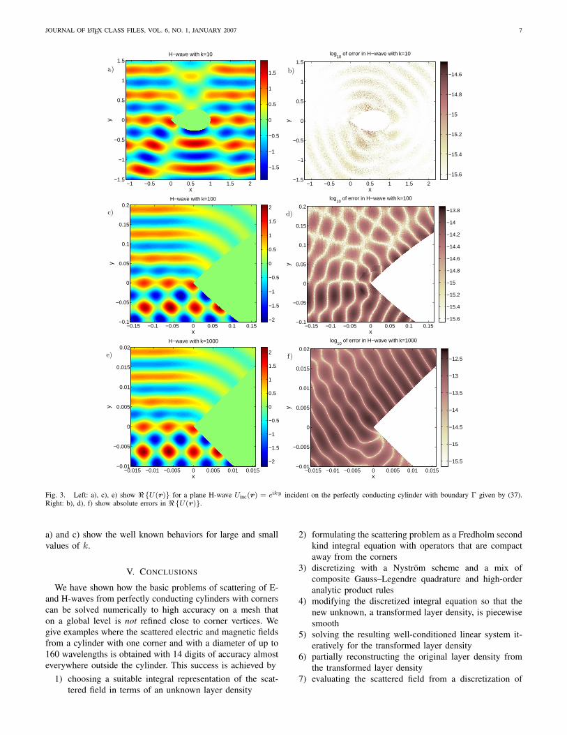
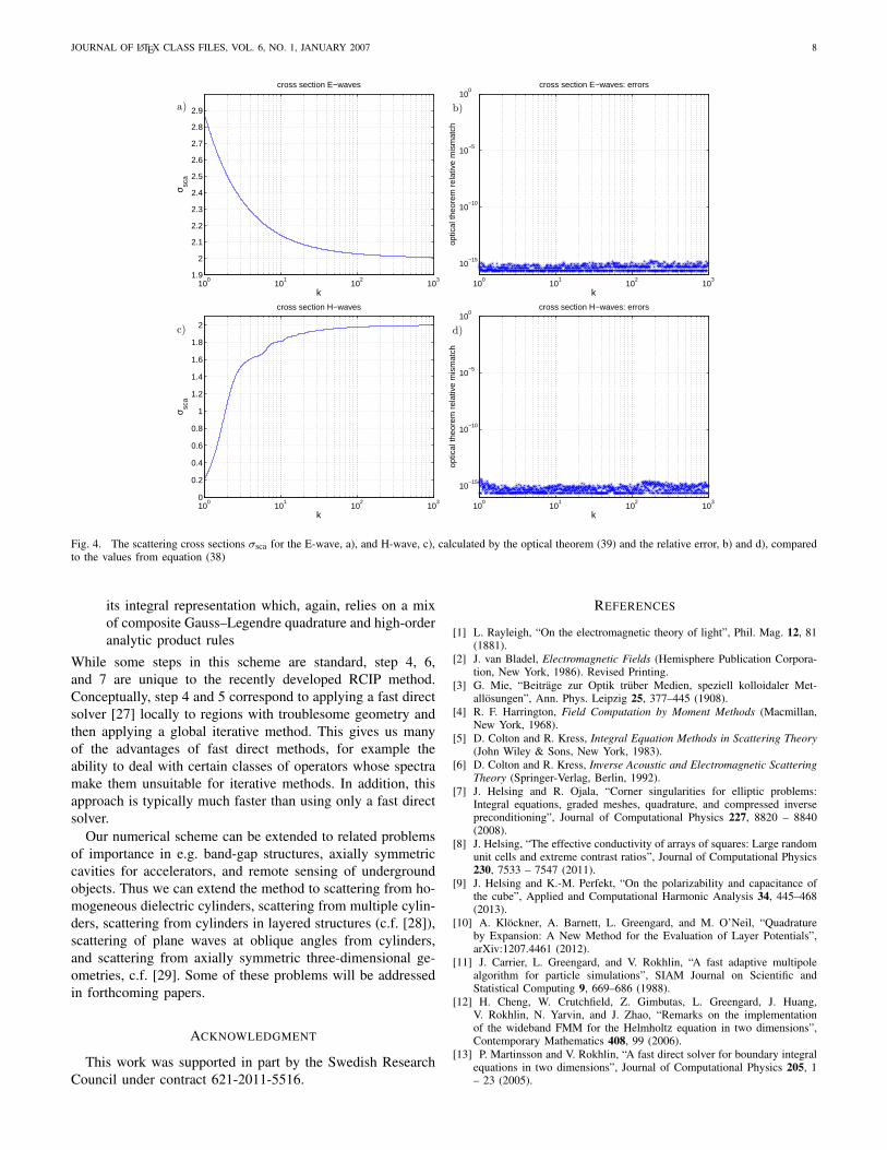
which should be even simpler to evaluate than (38) sinceit only involves the far field. The mismatch between thescattering cross sections computed via (38) and via (39) canbe used as an error estimate for both expressions. The crosssections for the E-waves along with such error estimates aregiven in Figure 4 a) and b) and the corresponding data forthe H-waves are given in Figures 4 c) and d). The mismatcherror is on the order of 10−15. The cross sections in Figures 4


x

y

H−wave with k=10

a)

−1 −0.5 0 0.5 1 1.5 2−1.5

−1

−0.5

0

0.5

1

1.5

−1.5

−1

−0.5

0

0.5

1

1.5

x

y

log10

of error in H−wave with k=10

b)

−1 −0.5 0 0.5 1 1.5 2−1.5

−1

−0.5

0

0.5

1

1.5

−15.6

−15.4

−15.2

−15

−14.8

−14.6

x

y

H−wave with k=100

c)

−0.15 −0.1 −0.05 0 0.05 0.1 0.15−0.1

−0.05

0

0.05

0.1

0.15

0.2

−2

−1.5

−1

−0.5

0

0.5

1

1.5

2

x

y

log10


d)

−0.15 −0.1 −0.05 0 0.05 0.1 0.15−0.1

−0.05

0

0.05

0.1

0.15

0.2

−15.6

−15.4

−15.2

−15

−14.8

−14.6

−14.4

−14.2

−14

−13.8

x

y

H−wave with k=1000

e)

−0.015 −0.01 −0.005 0 0.005 0.01 0.015−0.01

−0.005

0

0.005

0.01

0.015

0.02

−2

−1.5

−1

−0.5

0

0.5

1

1.5

2

x

y

log10


f)

−0.015 −0.01 −0.005 0 0.005 0.01 0.015−0.01

−0.005

0

0.005

0.01

0.015

0.02

−15.5

−15

−14.5

−14

−13.5

−13

−12.5

Fig. 3. Left: a), c), e) show <U(r) for a plane H-wave Uinc(r) = eiky incident on the perfectly conducting cylinder with boundary Γ given by (37).Right: b), d), f) show absolute errors in <U(r).

a) and c) show the well known behaviors for large and smallvalues of k.

V. CONCLUSIONS

We have shown how the basic problems of scattering of E-and H-waves from perfectly conducting cylinders with cornerscan be solved numerically to high accuracy on a mesh thaton a global level is not refined close to corner vertices. Wegive examples where the scattered electric and magnetic fieldsfrom a cylinder with one corner and with a diameter of up to160 wavelengths is obtained with 14 digits of accuracy almosteverywhere outside the cylinder. This success is achieved by

1) choosing a suitable integral representation of the scat-tered field in terms of an unknown layer density

2) formulating the scattering problem as a Fredholm secondkind integral equation with operators that are compactaway from the corners

3) discretizing with a Nystrom scheme and a mix ofcomposite Gauss–Legendre quadrature and high-orderanalytic product rules

4) modifying the discretized integral equation so that thenew unknown, a transformed layer density, is piecewisesmooth

5) solving the resulting well-conditioned linear system it-eratively for the transformed layer density

6) partially reconstructing the original layer density fromthe transformed layer density

7) evaluating the scattered field from a discretization of


100

101

102

103

1.9

2

2.1

2.2

2.3

2.4

2.5

2.6

2.7

2.8

2.9

cross section E−waves

k

σ sca

a)

100

101

102

103

10−15

10−10

10−5

100

cross section E−waves: errors

k

optic

al th

eore

m r

elat

ive

mis

mat

ch

b)

100

101

102

103

0

0.2

0.4

0.6

0.8

1

1.2

1.4

1.6

1.8

2

cross section H−waves

k

σ sca

c)

100

101

102

103

10−15

10−10

10−5

100

cross section H−waves: errors

k

optic

al th

eore

m r

elat

ive

mis

mat

ch

d)

Fig. 4. The scattering cross sections σsca for the E-wave, a), and H-wave, c), calculated by the optical theorem (39) and the relative error, b) and d), comparedto the values from equation (38)

its integral representation which, again, relies on a mixof composite Gauss–Legendre quadrature and high-orderanalytic product rules

While some steps in this scheme are standard, step 4, 6,and 7 are unique to the recently developed RCIP method.Conceptually, step 4 and 5 correspond to applying a fast directsolver [27] locally to regions with troublesome geometry andthen applying a global iterative method. This gives us manyof the advantages of fast direct methods, for example theability to deal with certain classes of operators whose spectramake them unsuitable for iterative methods. In addition, thisapproach is typically much faster than using only a fast directsolver.

Our numerical scheme can be extended to related problemsof importance in e.g. band-gap structures, axially symmetriccavities for accelerators, and remote sensing of undergroundobjects. Thus we can extend the method to scattering from ho-mogeneous dielectric cylinders, scattering from multiple cylin-ders, scattering from cylinders in layered structures (c.f. [28]),scattering of plane waves at oblique angles from cylinders,and scattering from axially symmetric three-dimensional ge-ometries, c.f. [29]. Some of these problems will be addressedin forthcoming papers.

ACKNOWLEDGMENT

This work was supported in part by the Swedish ResearchCouncil under contract 621-2011-5516.

REFERENCES

[1] L. Rayleigh, “On the electromagnetic theory of light”, Phil. Mag. 12, 81(1881).

[2] J. van Bladel, Electromagnetic Fields (Hemisphere Publication Corpora-tion, New York, 1986). Revised Printing.

[3] G. Mie, “Beitrage zur Optik truber Medien, speziell kolloidaler Met-allosungen”, Ann. Phys. Leipzig 25, 377–445 (1908).

[4] R. F. Harrington, Field Computation by Moment Methods (Macmillan,New York, 1968).

[5] D. Colton and R. Kress, Integral Equation Methods in Scattering Theory(John Wiley & Sons, New York, 1983).

[6] D. Colton and R. Kress, Inverse Acoustic and Electromagnetic ScatteringTheory (Springer-Verlag, Berlin, 1992).

[7] J. Helsing and R. Ojala, “Corner singularities for elliptic problems:Integral equations, graded meshes, quadrature, and compressed inversepreconditioning”, Journal of Computational Physics 227, 8820 – 8840(2008).

[8] J. Helsing, “The effective conductivity of arrays of squares: Large randomunit cells and extreme contrast ratios”, Journal of Computational Physics230, 7533 – 7547 (2011).

[9] J. Helsing and K.-M. Perfekt, “On the polarizability and capacitance ofthe cube”, Applied and Computational Harmonic Analysis 34, 445–468(2013).

[10] A. Klockner, A. Barnett, L. Greengard, and M. O’Neil, “Quadratureby Expansion: A New Method for the Evaluation of Layer Potentials”,arXiv:1207.4461 (2012).

[11] J. Carrier, L. Greengard, and V. Rokhlin, “A fast adaptive multipolealgorithm for particle simulations”, SIAM Journal on Scientific andStatistical Computing 9, 669–686 (1988).

[12] H. Cheng, W. Crutchfield, Z. Gimbutas, L. Greengard, J. Huang,V. Rokhlin, N. Yarvin, and J. Zhao, “Remarks on the implementationof the wideband FMM for the Helmholtz equation in two dimensions”,Contemporary Mathematics 408, 99 (2006).

[13] P. Martinsson and V. Rokhlin, “A fast direct solver for boundary integralequations in two dimensions”, Journal of Computational Physics 205, 1– 23 (2005).


[14] J. Bremer, “A fast direct solver for the integral equations of scatteringtheory on planar curves with corners”, Journal of Computational Physics231, 1879–1899 (2012).

[15] A. Gillman, P. Young, and P. Martinsson, “A direct solver withO(N) complexity for integral equations on one-dimensional domains”,Front. Math. China 7, 217 – 247 (2012).

[16] J. Helsing and R. Ojala, “Elastostatic computations on aggregates ofgrains with sharp interfaces, corners, and triple-junctions”, InternationalJournal of Solids and Structures 46, 4437 – 4450 (2009).

[17] J. Helsing, “Integral equation methods for elliptic problems with bound-ary conditions of mixed type”, Journal of Computational Physics 228,8892 – 8907 (2009).

[18] J. Helsing, “A fast and stable solver for singular integral equations onpiecewise smooth curves”, SIAM Journal on Scientific Computing 33,153–174 (2011).

[19] J. Helsing, “Solving integral equations on piecewise smooth boundariesusing the RCIP method: a tutorial”, Abstr. Appl. Anal. 2013, Article ID938167 (2013).

[20] J. L. Tsalamengas, “Exponentially converging Nystrom methods inscattering from infinite curved smooth strips–Part 1:TM-case”, IEEETrans. Antennas Propagat. 58, 3265–3274 (2010).

[21] J. L. Tsalamengas and C. V. Nanakos, “Nystrom solution to oblique scat-tering of arbitrarily polarized waves by dielectric-filled slotted cylinders”,IEEE Trans. Antennas Propagat. 60, 2802–2813 (2012).

[22] M. S. Tsong and W. C. Chew, “Nystrom method with edge conditionfor electromagnetic scattering by 2D open structures”, Progress in Elec-tromagnetics Research 62, 49–68 (2006).

[23] L. Greengard and J.-Y. Lee, “Stable and accurate integral equationmethods for scattering problems with multiple material interfaces in twodimensions”, Journal of Computational Physics 231, 2389 – 2395 (2012).

[24] O. Bruno, T. Elling, and C. Turc, “Regularized integral equations andfast high-order solvers for sound-hard acoustic scattering problems”,International Journal for Numerical Methods in Engineering 91, 1045–1072 (2012).

[25] R. Kress, “On the numerical solution of a hypersingular integral equationin scattering theory”, Journal of Computational and Applied Mathematics61, 345 – 360 (1995).

[26] S. Hao, A. H. Barnett, P. G. Martinsson, and P. Young, “High-orderaccurate Nystrom discretization of integral equations with weakly singularkernels on smooth curves in the plane”, arXiv:1112.6262v2 (2012).

[27] W. Y. Kong, J. Bremer, and V. Rokhlin, “An adaptive fast directsolver for boundary integral equations in two dimensions”, Applied andComputational Harmonic Analysis 31, 346 – 369 (2011).

[28] A. Karlsson, “Scattering from inhomogeneities in layered structures”,The Journal of the Acoustical Society of America 71, 1083–1092 (1982).

[29] J. L. Fleming, A. W. Wood, and W. D. Wood Jr. “Locally correctedNystrom method for EM scattering by bodies of revolution”, Journal ofComputational Physics 196.1, 41-52 (2004).

Johan Helsing was born in Stockholm, Sweden, in1961. He received his Ph. D. degree in TheoreticalPhysics from KTH, Stockholm, Sweden, in 1992.During 1992–1996 he held postdoctoral positions atthe Courant Institute, the University of Utah, and theRensselaer Polytechnic Institute. Since 2001 he is aProfessor at the Centre for Mathematical Sciences atLund University, Sweden. His research interests in-clude scientific computing, fast algorithms, integralequations, and potential theory.

Anders Karlsson was born in Goteborg, Swedenin 1955. He received his Ph. D. degree in Theo-retical Physics in 1984 from Chalmers Universityof Technology, Goteborg, Sweden. During 1985–1987 he was a postdoctoral fellow at the AppliedMathematical Sciences, Ames Iowa, USA. Since2000 he is a Professor in Electromagnetic Theoryat Lund University, Sweden. His research areas aredirect and inverse scattering, accelerators, and wavepropagation in dispersive materials.

JOURNAL OF LA An accurate boundary value problem solver ... · An accurate boundary value problem...

Documents

Transcript of JOURNAL OF LA An accurate boundary value problem solver ... · An accurate boundary value problem...