Journal of International Money and Finance 107 (2020) 102192

Contents lists available at ScienceDirect

Journal of International Money and Finance

journal homepage: www.elsevier .com/locate / j imf

Structural changes and the real exchange rate dynamicsq

https://doi.org/10.1016/j.jimonfin.2020.1021920261-5606/� 2020 Elsevier Ltd. All rights reserved.

q We would like to thank the editors, Kees Koedijk and Haoyuan Ding, and the anonymous referee for their helpful comments that led to siimprovements of the paper. Meanwhile, we wish to thank Shang-jin Wei and Michael Song for their helpful comments and discussions. We also tparticipants in the 2014 Econometric Society China Meeting, 2014 NBER-CCER Conference, 2014 Fudan Monetary Economics workshop, 201Congress (Jordan), and 2015 People’s Bank of China Macroeconomic Conference, as well as seminars held at Tsinghua University, Hong Kong Univethe Chinese University of Hong Kong. Qing Liu acknowledges the financial support of the National Natural Science Foundation of China (G71773060). Part of this work was conducted while Kang Shi was visiting the Hong Kong Institute for Monetary Research (HKIMR), whose suphospitality are greatly appreciated. All errors are the responsibility of the authors.⇑ Corresponding author.

E-mail addresses: jujd@pbcsf.tsinghua.edu.cn (J. Ju), justinlin@nsd.pku.edu.cn (J.Y. Lin), liuqing@sem.tsinghua.edu.cn (Q. Liu), kangshi@cuh(K. Shi).

Jiandong Ju a, Justin Yifu Lin b, Qing Liu c,⇑, Kang Shi d

a PBC school of Finance, Tsinghua University, Chinab Institute of New Structural Economics, Peking University, Chinac School of Economics and Management, Tsinghua University, ChinadDepartment of Economics, The Chinese University of Hong Kong, China

a r t i c l e i n f o a b s t r a c t

Article history:Available online 12 April 2020

JEL classification:F3F4O1O4

Keywords:Real exchange rateChinese economyExcess labor supplyH-O structure

Since China joined the WTO in 2001, the Chinese economy has grown very rapidly, espe-cially, the tradable goods sector. However, the Chinese real exchange rate did not exhibita persistent and stable appreciation until 2005. This is a puzzling fact that is inconsistentwith theories. This paper documents several stylized facts during the economic transitionand argues that two features of Chinese economy may help explain the puzzling realexchange rate pattern for Chinese economy: (i) the faster total factor productivity (TFP)growth in export sector compared with the import sector; (ii) excess supply of unskilledlabor. Our hypotheses are supported by cross-country evidence. Furthermore, we constructa small open economy model with an H-O trade structure and show that, due to heteroge-neous skilled labor intensity in export and import sectors, the faster TFP growth in theexport sector over that in the import sector will lead to the decline of return to capitaland the rise of skilled wage. Therefore, the decrease of return to capital and the lowunskilled wage, which is caused by the excess supply of unskilled labor, inhibit the risein the relative price of non-tradable goods to tradable goods as well as the appreciationof real exchange rate. Finally, we show that a dynamic small open economy model withmultiple tradable goods sectors does fairly well in explaining the Chinese real exchangerate and other stylized facts in the economic transition.

� 2020 Elsevier Ltd. All rights reserved.

1. Introduction

This paper investigates how structural changes in the labor market and traded-good sector help to explain the puzzlingdynamics of the real exchange rate in Chinese economy. According to the Balassa-Samuelson (BS) effect (Balassa, 1964;

gnificanthank the4 Worldrsity, andrant No.port and

k.edu.hk

2 J. Ju et al. / Journal of International Money and Finance 107 (2020) 102192

Samuelson, 1964), a positive relationship should be observed between the economic growth and the appreciation of the realexchange rate. The BS effect is driven by productivity catch-up in a developing country’s tradable sectors, which pushes upfactor prices and raises prices in non-tradable goods in the country. In the period of 2001–2007, China’s annual GDP growthreached an average of 11.2% and its annual growth rate of total trade is close to 20.2%. However, the China’s real exchangerate depreciated about 6.7% instead (labelled as Fact 1, see Figs. 1 and 2).

Several other stylized facts in China in this fast-growing period are also documented: significant current account surplus,considerable migration from rural to urban areas, the sharp rise in skilled wage premium, and lastly uneven technologicalprogress within the tradable goods sector (see Figs. 1–6). The first four facts have been well documented in literature, butthe final one has not been noted yet. Using Chinese manufacturing data and Chinese custom data, we find that during theperiod of 2001–2006, the TFP growth rate of the export sector is significantly higher than that of import sector.

How should we interpret these puzzling real exchange rate dynamics and the above stylized facts? The key to understandis the structural change. As a developing country, there was excess supply of unskilled labor in China, which keeps theunskilled wage at the minimum level. Assuming that the export sector is skilled labor intensive, the fast growing export sec-tor would induce large migration from rural to urban areas, and the sharp rise in skilled wage premium, the Facts 3 and 4.The import sector is more capital intensive. As the TFP growth rate of the export sector is significantly higher than that ofimport sector (Fact 5), using Stopler-Samuelson theorem, the return to capital may even decline, which results in capital out-flow and current account surplus (Fact 2). As the unskilled wage is at the minimum level and the capital return declines,assuming that the non-tradable sector uses little skilled labor, therefore, the price of non-tradable good could decline in thisfast growing period, so that real exchange rate depreciates (Fact 1).1

To test our intuition, we further investigate the effect of the difference in the TFP growth of the export and import sectorsas well as of the excess labor supply from rural to urban areas on the real exchange rate in developing countries. We conducta panel regression in the period of 1996–2013 for 82 economies. We augment the conventional empirical models on the realexchange rate by including two additional regressors: the urban–rural migration rate and the gap between the growth ratesof the export and import sectors. We find that an increase in migration rate by one standard deviation is associated with a28% depreciation in the RER. If the migration rate is at the level of one standard deviation, then an increase in the growth rateof the export sector relative to the import sector by one standard deviation is associated with a depreciation in RER of 3–4%.These data evidences support that the structural changes in labor market and in tradable sectors contribute significantly tothe real exchange rate dynamics in developing countries.

We then develop a theoretical framework to study such effects of structural changes on the real exchange rate dynamics.We first build two static models to explain the potential depreciation of the real exchange rate during this fast-growing per-iod. We then develop a dynamic small open economy model with an Hecksher-Ohlin structure. We consider two tradablesectors with heterogeneous factor intensity (the aforementioned H-O structure). We calibrate the model and show thatthe model can effectively explain the dynamics of the Chinese real exchange rate and other stylized facts documented forChinese economy during transition, such as the significant increase in skilled labor premium. In the model, the rapid TFPprogress in the export sector, which is supposedly labor intensive in China, also results in capital outflow, as observed inthe Chinese data. To generate the depreciation of real exchange rate, both abundant unskilled labor supply and the uneventechnological progress within the tradable good sector are essential. However, due to the fast economic development, ashortage of unskilled workers would be observed. This occurrence inevitably causes an increase in the unskilled wage, whichin turn boosts the prices of the non-tradable goods and then facilitates the appreciation of the real exchange rate. Thisimplies that the traditional Balassa-Samuelson (BS) mechanism works when there is no excess labor supply and theunskilled wage start to rise. Overall, our simulation results suggest that the real exchange rate exhibits an V-shape, whichis the pattern observed in the Chinese data.2

Our paper is closely related to the literature on the determination of real exchange rate. In this literature, there are twowell-known theories. The first one is the BS effect; the second one is the Froot-Rogoff effect, which postulates that the realexchange rate tends to rise with government consumption because government spending tends to fall disproportionately ondomestic non-tradable goods and services (Froot and Rogoff, 1991). According to Rogoff (1996), there are considerable,although not unanimous, empirical supports for both the Balassa-Samuelson effect and the Froot-Rogoff effect. For example,Beka et al., 2018 investigate the link between real exchange rates and sectoral TFP for Eurozone countries. They find that realexchange rate variation, both cross-country and time series, closely accords with an amended Balassa-Samuelson interpre-tation, incorporating sectoral productivity shocks and a labor market wedge. Recently, Du et al. (2013) argued that transportinfrastructure is an important determinant of the real exchange rate. The economic importance of the infrastructure effect isalmost on par with that of the well-known Balassa-Samuelson effect and is much greater than the Froot-Rogoff effect. In this

1 The heterogeneous skill intensity across tradable sectors is critical to account for the falling rental on capital thus the depreciating real exchange rate. As amatter of fact, the heterogeneous skill intensity across tradable sectors are well-documented in Chinese data. Moreover, there are also other evidence thatsupports the heterogeneous skill intensity among trade sectors and firms for other countries. For example, Bernard et al. (2007) for evidence for the U.S.,Verhoogen (2008) for Mexico, Alcala and Hernandez (2010) for Spain, Bustos (2011) for Argentina, Molina and Muendler (2013) for Brazil, and Eslava et al.(2015) for Colombia. In a recent work, Burstein and Vogel (2017) find strong evidence that the college intensity is positive correlated to the firm size.

2 Our benchmark model is simple; therefore, it can only match signs but not magnitudes. To match quantitatively with the Chinese data, we mustincorporate more realistic institution features or frictions into the model.

Fig. 2. Source: International Monetary Fund, International Financial Statistics. Real effective exchange rate index (2005 = 100).

Fig. 1. Source: National Bureau of Statistics of China.

J. Ju et al. / Journal of International Money and Finance 107 (2020) 102192 3

aspect, our paper also contributes to this literature, suggesting that migration and uneven development within tradable sec-tors might be important in affecting the real exchange rate dynamics.

Our work is related to a small but growing literature that considers multiple tradable sectors with different factor inten-sities in a general equilibrium framework. These papers include Cunat and Maffezzoli (2004), Ju and Wei (2007), Jin (2012),Jin and Li (2012), and Ju et al. (2012, 2014). Nevertheless, none of the existing works in this literature explicitly studies thereal exchange rate. To our best knowledge, there are few theories that accounts for Chinese real exchange rate.3 Most of thestudies on the Chinese real exchange rate are empirical; for example, Cheung et al. (2009) examine whether or not the Chineseexchange rate is misaligned and how Chinese trade flows respond to the exchange rate as well as to economic activity. Recently,Du and Wei (2013) presented a model with competitive saving motivation to show that the rise of sex-ratio may help explainthe decline of the real exchange rate in China. In our model, the structure changes caused by uneven technological progresswithin the traded goods sector and the migration of unskilled labor supply are the key to explaining the real exchange rate.

3 Existing literature pays little attention to the Chinese real exchange rate despite the substantial research on China’s current account imbalance during thatperiod, as conducted by scholars such as Song et al. (2011), Wei and Zhang (2011), and Ju et al. (2012). Our paper fills this gap.

4 J. Ju et al. / Journal of International Money and Finance 107 (2020) 102192

From the perspective of structural change, Wang et al. (2013) also attempted to use structural change to explain the US-Chinabilateral real exchange rate in a two-country model. However, they focused on the structural changes among agriculture, man-ufacturing, and service sectors, unlike our work. Compared with their work, our paper investigates not only the real exchangerate dynamics but also other stylized facts, such as capital outflow.

The rest of the paper is organized as follows. Section 2 documents the stylized facts during China’s fast-growing period.Section 3 presents cross-country empirical evidence. Section 4 presents static small open economy models of real exchangerate to show the model mechanism. Section 5 develops a dynamic model with an H-O structure to explain both the realexchange rate and current account dynamics. Section 6 reports the numerical results. Section 7 concludes this study.

2. Stylized facts during the transition of Chinese economy

In this section, we document a few stylized facts regarding the Chinese economy during its fast-growing period thatbegan in 2000.

1. V-shape exchange rate dynamics, in particular, no real exchange rate appreciation was observed during the fast-growingperiod (2001–2007)Given the fact of maintaining a high growth rate over a long period in China, a persistent real appreciation should beexpected. Fig. 2 shows that, however, the Chinese real exchange rate did not appreciate persistently until 2007. In par-ticular, we do not observe real exchange rate appreciation even after China joined the WTO in 2001 and the tradable sec-tor expanded dramatically. Instead, the real exchange rate depreciated at a rate of approximately 6.7% from 2001 to 2007.After 2007, the real exchange rate starts to appreciate. Thus, the real exchange rate exhibits a V-shape dynamics.

2. Significant trade balance and the rapid accumulation of foreign reservesSince 2001, the Chinese economy has been increasingly integrated into the world economy during its development. Theshare of international trade (export plus import) in GDP rose from less than 20% in the early 1980’s to almost 70% in 2007.During the process of China’s integrating into the world, we observed a considerable trade imbalance that has increasedrapidly, especially in recent years. As illustrated in Fig. 3, the annual average of the trade imbalance increased sharplywhen China joined the WTO; in 2007, China’s trade balance over GDP peaked at approximately 9%. Meanwhile, the coun-try also holds huge amount of foreign reserves that consists of roughly 50% of GDP. Such a significant trade imbalance hasgenerated a major political and economic issue between China and its trading partners; this situation has also initiated aseries of policy debates and academic controversies.

3. Considerable migration of unskilled labor from rural areas to the urban industryDuring China’s transition period, we observe the large-scale migration of unskilled labor from rural areas to the urbanindustry. A total of 2 million migrant workers, most of which were unskilled laborers, first migrated in 1978; this numbersurged up to 268 million in 2013. The mobilization of labor from rural areas provides an excess supply of unskilled laborto the industry, which in turn contributed to the persistent growth of the Chinese economy. Due to rapid economicgrowth, substantial reports or data have been presented regarding rising migrant wages (see Fig. 4), thus implying theshortage of unskilled labor in China. For example, according to the survey conducted by the CSSA, only 32% of firms couldhire sufficient workers in 2007. At least one third of the firms experienced labor supply shortage, with a gap higher than25%. Researchers such as Cai et al. (2007), Park et al. (2007), and Wang (2008), even argue that China has reached theLewis turning point.

4. Income inequality between skilled and unskilled workersChina’s economic transition is accompanied by increasing income inequality, especially in terms of wage inequalitybetween skilled and unskilled workers. Following Ge and Yang (2014), we use UHS data (1988–2012) to compute the skillpremium. The results are reported in Fig. 5, which also shows the trend of skill premium since 2000.4 This skill premiumincreased considerably after China’s entrance into theWTO, as widely documented in literature. However, the trend reversedin 2009; starting from this particular year, skill premium has declined rapidly from 0.474 to 0.393. 5

5. Higher TFP growth in exporting sectors than in importing sectorsThe growth rate of tradable sectors in China has remained high since 2001. If we decompose the aggregate TFP growth bysectors, the technological improvement across sectors follows the prevailing pattern of a fast-growing country, that is, thetradable goods sector grows faster than non-tradable goods sector does. Moreover, using the Chinese manufacturing dataand Chinese custom data, we compute the average TFP growth rate in export and import sectors during the period of2001–2006. Overall, the former is growing significantly faster than the latter is, as shown in Fig. 6. 6

4 Here the skilled labor includes high school and college education. We also compute the case in which skilled labor only covers those with college education,and the obtained results are similar.

5 The decline of skill premium also implies that there is no more excess supply of unskilled labor relative to the supply of skilled labor.6 Two methods (OP and ACF) are used to estimate sector-level TFP. The estimation process is detailed in Appendix. Results are similar in both method; for

simplicity, we report only the TFP estimated with the ACF method depicted in Fig. 6.

Fig. 3. Source: International Monetary Fund, Balance of Payments Statistics Yearbook and data files.

Fig. 4. Source: Zhao and Wu (2007) for 2003–6; Ministry of Agriculture (2010) for 2007–9.

J. Ju et al. / Journal of International Money and Finance 107 (2020) 102192 5

3. Cross-country evidence

Conducting a full-fledged cross-country estimation for the determinant of the real exchange rate is beyond the scope ofthis work. In this section, we present some empirical evidence supporting our aforementioned hypothesis, that is, the accel-erated TFP growth in the export sector over that in the import sector and the abundant unskilled labor supply depress realexchange rate appreciation.

3.1. Estimation equations

At this point, we investigate the effect of the difference in the TFP growth of the export and import sectors as well as of theexcess labor supply from rural to urban areas on the real exchange rate. We augment existing empirical models on the realexchange rate by including two additional regressors: the urban–rural migration rate and the gap between the growth ratesof the export and import sectors. The latter is a proxy for the TFP difference between the export and import sectors. Conven-tional panel regressions with country and year fixed effects are presented as well.

Our estimation specification is as follows:

log RERð Þi;t ¼ aþ b1migrationi;t þ b2diff eximit þ b3diff eximit �migrationi;t þ Xi;t þ di þ ft þ eit

Fig. 5. Source: UHS data, computation results from Bai et al., 2020.

Fig. 6. Source: Author’s Computation using the Chinese manufacturing data and Chinese custom data.

6 J. Ju et al. / Journal of International Money and Finance 107 (2020) 102192

where log RERð Þi;t refers to the log of real exchange rate of country i in year t, migrationi, t is the rural–urban migration rate ofcountry i, diff_eximit is determined by subtracting export growth rate from the import growth rate, and diff_eximit⁄migra-tioni, t is an interaction term. Xi;t denotes other determinants of the RER, which includes GDP per capita, government expen-diture/GDP, terms of trade, net foreign asset/GDP, real interest rate, and tariff rate. The choice of control variables is guidedby Rogoff (1996), the International Monetary Fund (2006), and Du et al. (2013). di captures the country effect and ft the yeareffect.

3.2. Data description

We start with data for 248 economies worldwide over the period of 1996–2013. However, as some observations drop outdue to missing values in different variables, we conduct the panel regression in this period for 82 economies, 70 countries,

J. Ju et al. / Journal of International Money and Finance 107 (2020) 102192 7

and 67 countries, as listed in Columns 1, 3–5, and 6, respectively. A list of countries is provided in the Appendix A forTable A1. The definitions and descriptive statistics for key variables of interest are presented in Table 1; additional details,including data sources, are shown in the Appendix A for Table A2.

Our independent variable is a country’s real exchange rate (RER). Our measure of RER is the real effective exchange rateindex of the International Monetary Fund, which is constructed by dividing the nominal effective exchange rate (a measureof the value of a currency against a weighted average of several foreign currencies) with a price deflator or index of costs.Since the nominal exchange rate enters the index in its inverse form, we inverse the term so that a rise in RER denotes realdepreciation; this notation is consistent with the conventional definition of the real exchange rate in our model. Note thatthe base year is 2010; as a result, only changes in log of RER, rather than in its absolute value, matter in cross-country com-parison. In panel data, this issue is absorbed by the country fixed effects.

We utilize two key regressors. The first one is the urban–rural migration rate. We adopted the method of regional scienceto compute the country-level rural outmigration rate. The underlying assumption that total population growth does notstray too far from natural urban population growth appears to be rather strong at first glance; however, a close look at evi-dence suggests that the differences tend to be slight, at least for cross-country studies. The data for total population growth,urban population growth, and urban ratio are all available in the World Bank’s World Development Indicator (WDI).

The second key regressor is an interaction term, which is the gap between the export and import growth rates multipliedby the migration rate. According to our hypothesis, the technological improvement in the export sector alone does notinduce real exchange rate depreciation. It is the coexistence of abundant unskilled labor and uneven technological improve-ment within tradable sectors is able to break down the Balassa-Samuelson effect. The data for export and import growthrates both originate from WDI.

We follow existing literature on the determinants of RER and include the following control variables: income per capita,government expenditure, net foreign assets, commodity terms of trade, real interest rate, and trade restriction. The detaileddata sources of these variables are listed in the Appendix A for Table A2.

3.3. Panel regression results

Table 2 reports the panel regression results. Both country fixed effects and year fixed effects are included. Following Duet al. (2013), we re-scale all the regressors by their standard deviations in the sample so that the magnitudes of the coeffi-cients on variables become comparable with one another. Robust standard errors are clustered by country.

As per Column 1 of Table 2, migration rate alone is included as the key regressor aside from the control variables. Thecoefficient on migration is statistically significant and takes a positive sign. In accordance with our theory, an increase inmigration rate by one standard deviation is associated with a 28% increase in the RER. In comparison, an improvement inper capita income by one standard deviation is associated with 49% real appreciation (Balassa-Samuelson effect). A rise ingovernment expenditure shares by one standard deviation is associated with an 7% appreciation in RER (Froot-Rogoff effect).These estimates suggest that the economic significance of urban–rural migration can be greater than half the Balassa-Samuelson effect and roughly four times stronger than the Froot-Rogoff effect.

According to Column 2 of Table 2, only export growth rate minus import growth rate is included aside from the controlvariables. The coefficient takes the expected sign, although this value is not significant. Based on Column 3, the coefficients ofthe two regressors do not change much when both migration rate and export growth rate minus import growth rate areincluded. Nonetheless, the potential explanatory power of the new variable is highlighted by a substantial increase in R-squared from approximately 0.20 to 0.35 and an enhancement in the significance level of the migration rate from 10% to 1%.

As per Column 4 of Table 2, an interaction term of migration rate and export growth rate minus import growth rate isincluded aside from the two regressors and in combination with other control variables. The coefficient on the interactionterm is statistically significant and takes a positive sign, whereas the coefficient on migration rate is not significantlyaffected. This outcome suggests that the gap between the export and import sectors in technological progress can only influ-ence the RER through surplus labor. That is, when migration rate is equal to zero, the TFP growth gap within sectors has nosignificant effect on real exchange rate. Specifically, if migration rate is at the level of one standard deviation, then anincrease in the growth rate of the export sector relative to the import sector by one standard deviation is associated with

Table 1Definition and summary statistics of key variables for cross countries (1996–2013).

Variable Definitions Variable Names Obs Mean Std. Dev. Min Max

RER = Real Exchange Rate Log (100/REER⁄100) 1689 4.56 0.24 2.28 5.60Migration Rate = (lt � qtÞut/(1-ut) Migration Rate 4278 0.98 5.51 �5.08 350.72Export_Import_Developing = Export growth rate – import growth rate Diff_exim 2835 �0.26 7.50 �20.45 21.57Log GDP per capita in 2011 PPP dollars Log GDP/capita 3942 8.98 1.22 5.02 11.84GOV/GDP = (government expenditure/GDP) GOV/GDP 3676 16.19 7.96 2.05 156.53Terms of Trade (ToT)= Net barter terms of trade index (2000 = 100) Terms of Trade 3105 108.17 32.19 21.22 262.09Net Foreign Asset/GDP NFA/GDP 3126 0.25 0.82 �1.98 14.06Real Interest Rate, in % Real Interest Rate 2565 8.14 20.07 -96.87 572.94Tariff Rate = Trade weighted applied tariff rate, in percentage points Tariff Rate 2108 7.22 8.87 0.00 254.58

Data Sources: For detailed information on data sources and definition of terms, please refer to Appendix Table 2.

Table 2Panel regressions.

Dependent Variable Log Real Exchange Rate(Index 2010 = 100)

(1) (2) (3) (4) (5) (6)

Migration Rate 0.283⁄ 0.274⁄⁄⁄ 0.267⁄⁄⁄ 0.265⁄⁄⁄ 0.136⁄⁄⁄(0.148) (0.0898) (0.0915) (0.0923) (0.0344)

Diff_exim 0.00612 0.00613 0.00225 1.34e-05(0.00534) (0.00537) (0.00581) (0.00587)

Diff_exim ⁄Migration Rate 0.0322⁄ 0.0384⁄⁄ 0.0534⁄⁄⁄(0.0184) (0.0190) (0.0175)

lgdp_pcsd �0.493⁄⁄⁄ �0.507⁄⁄⁄ �0.546⁄⁄⁄ �0.544⁄⁄⁄ �0.543⁄⁄⁄ �0.330⁄⁄(0.0756) (0.105) (0.107) (0.105) (0.105) (0.136)

gov_gdpsd �0.0698⁄⁄ �0.102⁄ �0.105⁄ �0.103⁄ �0.102⁄ 0.0258(0.0335) (0.0560) (0.0566) (0.0571) (0.0574) (0.0258)

totsd �0.0229 �0.0417⁄⁄ �0.0340⁄⁄ �0.0348⁄⁄ �0.0350⁄⁄ �0.000561(0.0259) (0.0161) (0.0169) (0.0171) (0.0172) (0.0293)

nfa_gdpsd 0.0983⁄⁄ 0.147⁄⁄ 0.144⁄⁄⁄ 0.145⁄⁄⁄ 0.144⁄⁄⁄ 0.0469⁄⁄(0.0413) (0.0556) (0.0508) (0.0516) (0.0514) (0.0230)

rirsd �0.00195 �0.0454 �0.0439 �0.0447 �0.0444 �0.0265⁄⁄(0.0178) (0.0302) (0.0287) (0.0283) (0.0283) (0.0122)

tariffsd �0.0554 �0.0312 �0.0306 �0.0322 �0.0323 0.0230(0.0348) (0.0474) (0.0469) (0.0470) (0.0470) (0.0163)

Observations 710 599 585 585 585 448R-squared 0.198 0.331 0.348 0.350 0.350 /Number of id 82 71 70 70 70 67Country FE YES YES YES YES YES /Year FE YES YES YES YES YES YES

Robust standard errors in parentheses ⁄⁄⁄ p<0.01, ⁄⁄ p<0.05, ⁄ p<0.1.

8 J. Ju et al. / Journal of International Money and Finance 107 (2020) 102192

a depreciation in RER of 3%-4% (as suggested by the true model presented in Column 5); this occurrence is comparable withthe economic effect of the terms of trade. Furthermore, if migration rate is as high as two standard deviation levels, then theinfluence of the TFP growth rate gap is also doubled, and so forth.

3.4. Robustness check

We acknowledge that there could be endogeneity problem resulting from simultaneity between RER and the growth ofexport and import. Furthermore, we recognize that another instance of endogeneity can arise from the possibility that cur-rent growth in export and import are not independent of past RERs. To control for such dynamic endogeneity and simultane-ity, we employ the generalized method of moments (GMM) estimation procedure for dynamic panels as introduced byArellano and Bond (1991) to our panel. Past values of RER and export growth minus import growth are used as internalinstruments for current export growth minus import growth. This eliminates the need for external instruments (Wintoki,et al., 2012).

First, we rewrite the regression model as a dynamic model that includes lagged RER as explanatory variables. Second, weempirically examine how many lags are required. Glen et al. (2001) and Gschwandtner (2005) suggest that two lags are suf-ficient to capture the persistence of dependent variables. To confirm if two lags can ensure dynamic completeness, we esti-mate a model with three lags and find that indeed, the first lag alone is statistically significant; other lags are insignificant.7

Third, we apply the three higher lags of the endogenous variable, the Export_Import term as its own instruments. Finally, weestimate a one-step dynamic GMM estimator with robust stand error clustering on countries. The results are appended in Col-umn 6 of Table 2. The Arellano-Bond test for the AR(1) first-order serial correlation tests yields a p-value of 0.0003, as expectedfor differenced errors. The AR(2) second-order serial correlation test generates a p-value of 0.1168 that fails to reject the nullhypothesis of no second-order serial correlation. The Sargan test of over-identification produces a p-value of 0.2612; thereforewe cannot reject the hypothesis that our instruments are valid.8 Our baseline results hold qualitatively in this dynamic panelGMM regression setup, although the magnitude of coefficients varies slightly. We thus conclude that surplus labor and thehigher growth of the export sector relative to the import sector may depress RER appreciation.

4. Static models

In this section, we set up two static models to reveal the main channels that we focus in this paper. To highlight the role ofthe two important features of China’s transition, namely, the excess supply of unskilled labor and the uneven technologicalprogress within the tradable goods sector, we begin with the two-sector model.

7 In the table, the coefficients for lagged RER are suppressed because they are not of interest, but these coefficients are available upon request.8 We also conduct the system GMM introduced by Arellano and Bover (1995) and Blundell and Bond (1998) with the xtabond2 command in STATA. This

approach yields Hansen J test, which is robust to heteroskedasticity. The results are qualitatively similar.

J. Ju et al. / Journal of International Money and Finance 107 (2020) 102192 9

4.1. Two-sector model with ‘‘Surplus Labor”

Underlying the Balassa-Samuelson effect is the wage linkage across sectors. The technological improvement in the trad-able sector increases the marginal product of labor for workers and boosts real wages. Wages are equalized across sectors asa result of labor mobility; therefore, wages in the non-tradable goods sector also increases and boosts the price for non-tradable goods. In the process, real appreciation is observed along with TFP growth. Notably, the rise in wages is the keychannel to generate the Balassa-Samuelson effect in the benchmark model. This channel may be insignificant when weobserve abundant supplies of labor.

Consider a small open economy where the final good is a Cobb-Douglas aggregation of tradable and non-tradable goods.

The aggregate price is simply given by P ¼ PTð Þh PNð Þ1�h, where PT and PN (T refers to the tradable goods sector and N to thenon-tradable goods sector) are the prices of tradable and non-tradable goods, respectively. In such a setting, the realexchange rate can be measured by the relative price of non-tradable to tradable goods. For simplicity, we regard the tradablegoods as the numeraire, and its price is normalized to 1 so that PN can reflect the movement of the real exchange rate. Thetechnologies applied in the two sectors are given as follows:

9 Whmobilitgoods. I

Yi ¼ AiLi

1� ai

� �1�ai Ki

ai

� �ai; ð4:1Þ

where i ¼ T;Nf g denotes the sector i. Li denotes the labor used in sector i;Ki is the capital used in sector i, and Ai is the TFP insector i, respectively. In accordance with the literature, we assume that aT > aN , that is, that the non-tradable goods sector ismore labor intensive than the tradable goods sector is.

In a competitive equilibrium, we obtain the following optimal conditions:

1 ¼ wð Þ1�aT raTAT

; ð4:2Þ

PN ¼ wð Þ1�aN raNAN

; ð4:3Þ

where r is the return to capital and w is the wage of labor.We consider an economy with ‘‘surplus labor” from rural areas, and assume an exogenous minimum wage level wmin.

Therefore, the equilibrium for this economy is characterized by Eqs. (4.2) and (4.3) as well as two additional constraints:

w ¼ wmin; ð4:4Þ

LT þ LN < L; ð4:5Þ

where L is total labor supply in this economy. In equilibrium, we can solve for return to capital as follows:9

r ¼ wminð Þ1� 1aT ATð Þ 1

aT ; ð4:6Þ

and the price of the non-tradable goods is simply given as follows:

PN ¼ /2ATð Þ

aNaT

AN: ð4:7Þ

where /2 ¼ wminð Þ1�aNaT > 0. On the basis of Eq. 4.7, we establish the following proposition.

Proposition 1. Consider an economy with ‘‘surplus labor”. If the growth rate of technology in the tradable goods and non-tradablegoods sectors satisfy the following condition g ATð Þ

g ANð Þ >aTaN > 1, the (weaken) Balassa-Samuelson effect remains and real exchange rate

appreciates with technology improvements.

The proof is trivial and the intuition is straightforward: although the wage of labor is depressed to the minimum level,technological improvement drives up the demand for capital, which in turn boosts the real interest rate and increases theprice of non-tradable goods. Note that PN would drop if all sectors grow at the same rate. So result differs from that ofthe benchmark model of BS effect, where the real exchange rate appreciates as long as AT > AN . This outcome implies thatif the technologies in both sectors improve, the price of non-tradable goods does not rise unless the tradable sector growsmuch faster than the non-tradable sector does. Therefore, introducing ‘‘surplus labor” into the benchmark model exerts anew effect on real exchange rates; nevertheless, a weak version of the Balassa-Samuelson effect remains.

en the wage is depressed to the minimum level, the small open economy cannot take the world interest rate as given. There must be imperfect capitaly across border. Therefore, the domestic return to capital can be determined endogenously, which guarantees the economy to produce both tradablen this setting, the return to captial is the key to generate BS effect.

10 J. Ju et al. / Journal of International Money and Finance 107 (2020) 102192

4.2. Three-sector model with ‘‘Surplus Labor”

In this section, we propose a novel mechanism through which the Balassa-Samuelson effect may fail and a rapid growingeconomymay still experience real depreciation as well as current account surplus. To provide a transparent quantification ofthis new channel, we now introduce the Hecksher-Ohlin structure into the model. In particular, there are two tradable sec-tors that produce good 1 and good 2, and one nontradable sector that produces nontradable good 3. Skilled labor, unskilledlabor and capital are available for production. Now the productions in both tradable and nontradable sectors use all the threefactors. Therefore, the production functions in the four sectors are simply given by

Yit ¼ AitNit

bi

� �bi Litai

� �ai Kit

ci

� �ci; ð4:8Þ

where i ¼ 1;2;Nf g denotes sector i;ai; bi, and ci are the unskilled labor income share, skilled labor income share, and capitalincome share in sector i, respectively. More specifically, the two tradable sectors, sector 1 and sector 2, are export and importsectors, respectively; sector N is the non-tradable sector.

Let pi denotes the price of goods i. Then firm’s optimal decisions on factor allocation give us

wtLit ¼ aipitYit; stNit ¼ bipitYit ; andrtKit ¼ cipitYit : ð4:9Þ

We can rewrite above Eqs. (4.9) as the following:

pit ¼wtð Þai stð Þbi rtð Þci

Ait: ð4:10Þ

Let x ¼ DX=X denotes the ralative change of variable X. We can rewrite Eq. (4.10) as the following:

pit ¼ aiwt þ bi st þ ci rt � ait: ð4:11Þ

Since this is a small open economy, the prices of tradable goods, p1t and p2t , is exogenously determined by the world market.Moreover, we focus on the scenario where there is excess labor supply. Therefore, wt ¼ wmin in equilibrium. Therefore, wehave

pit ¼ 0; ð4:12Þ

and

wt ¼ 0: ð4:13Þ

Put Eqs. (4.12) and (4.13) into (4.11), we have

rt ¼ �1b1a1t � 1

b2a2t

c2b2� c1

b1

; ð4:14Þ

Thus, as long as the export sector is relatively more unskilled labor intensive than the import sector, i.e., c2b2 >c1b1, the increase

in A1t will lead to the decline of return to capital. This result is essentially a corollary from the Stolper-Samuelson theorem.The intuition is straightforward: Since sector 1 is relatively more labor intensive, the technological progress in sector 1reduces the relative demand of capital, and thereby leads to a fall in the rental rate of capital.

The price of non-tradable goods is endogenously determined, and it can be written as follows,

pN ¼bNb1

c2b2� cN

b1c2b2� c1

b1

a1t þ bN

b2

cNbN

� c1b1

c2b2� c1

b1

a2t � a3t: ð4:15Þ

The above equation implies that as long as the skilled labor income share in the non-tradable sector, bN , is not too high, aTPF growth in sector 1 can generate a decline in the price of non-tradable goods. Since the aggregate price is given by

P ¼ p1ð Þh1 p2ð Þh2 pNð Þ1�h1�h2 , where h1 and h2 are the shares of two tradable goods in the final goods, and both p1t and p2t

are exogenously given, a decline in p3t indicates a real depreciation. Thus, our mechanism provide an opposite predictionon the real exchange rate compared to traditional Balassa-Samuelson effect.

In particular, define the skilled labor income share b�N � cN

c2b2. We need bN < b�

N so that our mechanism dominates. Note

that the condition bN > b�N is equivalent to bN

cN< b2

c2. Therefore, as long as the non-tradable sector is less skilled intensive than

the import sector (and thus the export sector as well), the rapid growth in export sector induces the real depreciation. Thisfinding suggests that uneven technology progress within the tradable sector and the abundant labor supply may reverse theBalassa-Samuelson effect.

We summarize the above findings as follows:

J. Ju et al. / Journal of International Money and Finance 107 (2020) 102192 11

Proposition 2. With excess supply of labor, the technological improvement in the more (less) labor-intensive tradable sector willlead to the decline (rise) of return to capital. Moreover, if non-trable sector is less (more) skilled intensive than the tradable sector,the real exchange rate will depreciate (appreciate).

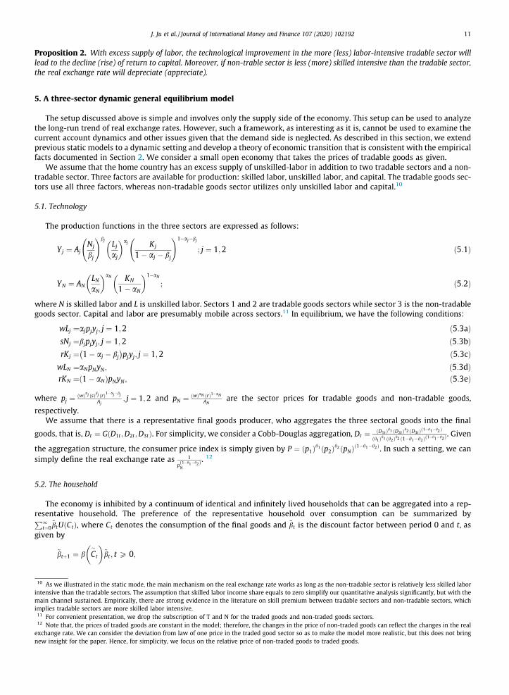
5. A three-sector dynamic general equilibrium model

The setup discussed above is simple and involves only the supply side of the economy. This setup can be used to analyzethe long-run trend of real exchange rates. However, such a framework, as interesting as it is, cannot be used to examine thecurrent account dynamics and other issues given that the demand side is neglected. As described in this section, we extendprevious static models to a dynamic setting and develop a theory of economic transition that is consistent with the empiricalfacts documented in Section 2. We consider a small open economy that takes the prices of tradable goods as given.

We assume that the home country has an excess supply of unskilled-labor in addition to two tradable sectors and a non-tradable sector. Three factors are available for production: skilled labor, unskilled labor, and capital. The tradable goods sec-tors use all three factors, whereas non-tradable goods sector utilizes only unskilled labor and capital.10

5.1. Technology

The production functions in the three sectors are expressed as follows:

10 As wintensivmain chimplies11 For12 Notexchangnew ins

Yj ¼ AjNj

bj

!bjLjaj

� �aj Kj

1� aj � bj

!1�aj�bj

; j ¼ 1;2 ð5:1Þ

YN ¼ ANLNaN

� �aN KN

1� aN

� �1�aN; ð5:2Þ

where N is skilled labor and L is unskilled labor. Sectors 1 and 2 are tradable goods sectors while sector 3 is the non-tradablegoods sector. Capital and labor are presumably mobile across sectors.11 In equilibrium, we have the following conditions:

wLj ¼ajpjyj; j ¼ 1;2 ð5:3aÞsNj ¼bjpjyj; j ¼ 1;2 ð5:3bÞrKj ¼ 1� aj � bj

� �pjyj; j ¼ 1;2 ð5:3cÞ

wLN ¼aNpNyN ; ð5:3dÞrKN ¼ 1� aNð ÞpNyN; ð5:3eÞ

where pj ¼ wð Þaj sð Þbj rð Þ1�aj�bj

Aj; j ¼ 1;2 and pN ¼ wð ÞaN rð Þ1�aN

ANare the sector prices for tradable goods and non-tradable goods,

respectively.We assume that there is a representative final goods producer, who aggregates the three sectoral goods into the final

goods, that is, Dt ¼ G D1t ;D2t ;D3tð Þ. For simplicity, we consider a Cobb-Douglas aggregation, Dt ¼ D1tð Þh1 D2tð Þh2 D3tð Þ 1�h1�h2ð Þh1ð Þh1 h2ð Þh2 1�h1�h2ð Þ 1�h1�h2ð Þ. Given

the aggregation structure, the consumer price index is simply given by P ¼ p1ð Þh1 p2ð Þh2 pNð Þ 1�h1�h2ð Þ. In such a setting, we cansimply define the real exchange rate as 1

p1�h1�h2ð ÞN

. 12

5.2. The household

The economy is inhibited by a continuum of identical and infinitely lived households that can be aggregated into a rep-resentative household. The preference of the representative household over consumption can be summarized byP1

t¼0~btU Ctð Þ, where Ct denotes the consumption of the final goods and ~bt is the discount factor between period 0 and t, as

given by

~btþ1 ¼ b C�t

� �~bt; t P 0;

e illustrated in the static mode, the main mechanism on the real exchange rate works as long as the non-tradable sector is relatively less skilled labore than the tradable sectors. The assumption that skilled labor income share equals to zero simplify our quantitative analysis significantly, but with theannel sustained. Empirically, there are strong evidence in the literature on skill premium between tradable sectors and non-tradable sectors, whichtradable sectors are more skilled labor intensive.convenient presentation, we drop the subscription of T and N for the traded goods and non-traded goods sectors.e that, the prices of traded goods are constant in the model; therefore, the changes in the price of non-traded goods can reflect the changes in the reale rate. We can consider the deviation from law of one price in the traded good sector so as to make the model more realistic, but this does not bringight for the paper. Hence, for simplicity, we focus on the relative price of non-traded goods to traded goods.

12 J. Ju et al. / Journal of International Money and Finance 107 (2020) 102192

where ~b0 ¼ 1 and bC� < 0. We assume that the endogenous discount factor does not depend on the consumption of an indi-

vidual household, but rather on the average per capita consumption C�, which an individual household takes as given. This

preference specification was originally proposed by Uzawa, 1968 and was introduced into the small open economy literatureby Mendoza, 1991.

The budget constraint and capital accumulation are expressed as follows:

PtCt þ PtIt þ PtBtþ1 þ Ptw2

Btþ1 � B� �2 ¼ stNt þwtLt þ rtKt þ 1þ r�ð ÞPtBt; ð5:4Þ

1� dð ÞKt þ It ¼ Ktþ1: ð5:5Þ

where Nt denotes skilled labor, Lt indicates unskilled labor, and r� is the world interest rate, which is taken as given in oursmall open economy setup.

The first-order conditions with respect to Ct;Ktþ1, and Btþ1 yield the following:

U0 Ctð Þ 1þ w Btþ1 � B� �� � ¼ 1þ r�ð Þb C

�t

� �U0 Ctþ1ð Þ; ð5:6Þ

U0 Ctð Þ ¼ b C�t

� �U0 Ctþ1ð Þ 1� dþ rtþ1

Ptþ1

� : ð5:7Þ

By using Eqs. (5.6) and (5.7), we immediately obtain

1þ w Btþ1 � B� � ¼ 1þ r�

1� dþ rtþ1=Ptþ1; ð5:8Þ

Therefore, households will choose to purchase additional foreign assets when the domestic interest rate decreases, thusresulting in capital inflow and current account surplus.

5.3. Characterization of equilibrium

Now we are ready to characterize a competitive equilibrium. We first denote the aggregate demand of domestic resi-dences for final goods as below

Dt ¼ Ct þ It þ w2

Btþ1 � B� �2

: ð5:9Þ

Therefore, the domestic demands for tradable and non-tradable goods are given as follows, respectively,

D1t ¼h1PtDt

p1t; ð5:10Þ

D2t ¼h2PtDt

p2t; ð5:11Þ

DNt ¼ 1� h1 � h2ð Þ PtDt

pNt: ð5:12Þ

Let production in each sector j be Yj. Then market clear condition for non-tradable goods requires:

YNt ¼ DNt: ð5:13Þ

The domestic factor markets also clear, implying that

N1 þ N2 ¼ N; ð5:14Þ

K1 þ K2 þ KN ¼ K; ð5:15Þ

L1 þ L2 þ LN 6 L: ð5:16Þ

We divide the transition of the economy into two stages. At the first stage when TFP level is low, there are abundant

unskilled labor, hence, L1 þ L2 þ LN < L. The wage of unskilled workers is fixed at the minium level wmin. As TFP keeps grow-ing, the economy enters into the second stage and the excess unskilled labor supply disappears. The wage of unskilled work-ers starts to grow with the technology improvement. To simplify the analysis, we assume that the wage of unskilled workersw exogeneously increases as TFP grows at the second stage.

The pattern of unskilled labor wage is imposed exogenously in this section. We can endogenize such structure by intro-ducing an agriculture sector into the economy. In the first stage, there exists excess unskilled labor in the agriculture sector,which implies that the unskilled labor will only be compensated by minimum wage. When the economy enters into thesecond stage, the unskilled labor constraint binds, and after which the unskilled wage rises endogenously with technology

J. Ju et al. / Journal of International Money and Finance 107 (2020) 102192 13

progress. In Technical Appendix B, we formally develop the extended model and show that the unskilled wage dynamics pre-sents the same pattern as that assumed in this section.

Finally, a competitive equilibrium consists of a set of prices, allocation rules, and trade shares, such that: (1) given theprices, all firm’s inputs satisfy the FOCs and the outputs are given by the production functions. (2) Given the prices, the con-sumers’ demand satisfies the first-order conditions derived from the household’s problem, and the bonds holdings satisfy theasset pricing rule (5.8). (3) The prices ensure the market clearing conditions for labor, capital, non-tradable goods, and thehousehold budget constraint.

6. Quantitative analysis

6.1. Calibration

Our model is calibrated at annual frequency. The parameter values are summarized in Table 3. We assume the period

utility function u cð Þ ¼ C1�c1�c , where the inverse of the elasticity of intertemporal substitution c ¼ 2. The steady state discount

factor b ¼ 0:96, which implies a 4% annual world interest rate. Following Choi et al., 2008, the endogenous time discount

factor takes the function form b C�t

� �¼ b

~Ct

C

��/, where / ¼ 0:1.

We assume that non-tradable goods constitute approximately 50% of the final goods and that the tradable goods haveequal share in the final good; this implies that h1 ¼ h2 ¼ 0:25. We set the production parameters as follows:a1 ¼ 0:35; b1 ¼ 0:35;a2 ¼ 0:1; b2 ¼ 0:1;aN ¼ 0:65 such that the average capital shares in the tradable and non-tradable goodssector are 0.55 and 0.35, respectively;These shares are similar to those estimated from China’s input–output table in 2002.The annual depreciation rate of capital dis set to 0:1. Following Schmitt-Grohe and Uribe (2003), the coefficient for bondadjustment costs wb is set to 0:0007. For simplicity, the value of the skilled-labor supply N is normalized to 1.

It is assumed that sectoral productivity A1 ¼ A2 ¼ AN ¼ 1 in the initial steady state. We further choose the prices of trad-able goods prices to make r ¼ r� so that B ¼ 0 in the initial period. Given the prices, we pin down the initial unskilled-wage,which is assumed to be exogenous in the model. The numerical methods for solving steady state and transition dynamics arepresented in Technical Appendix A.

6.2. Results

As explained in this section, we evaluate the model quantitatively. Note that we are interested in the dynamics of the realexchange rate and current account in an economy featured with abundant unskilled labor supply as well as the experience offast TFP growth in tradable sectors. Thus, we consider that our modeling economy starts from the initial steady state whileA1 ¼ 1and transits to the new steady state with A1 ¼ 1:04 while A2and AN remain unchanged.13 We solve the transitiondynamics with the shooting algorithm.

6.2.1. TFP shocks and wage structureBased on the evidence we described in Section 2, the exporting sector generically grows faster than importing sector does

while China has maintained a high growth rate in the tradable goods sectors since 2001 (see Fig. 6). Moreover, the supply ofunskilled labor from rural areas has continually increased since the early 1990s, which drives the upward trend of skill pre-mium. Significant controversies have arisen on whether or not China has reached the Lewis turning point, that is, whether ornot an excess supply of unskilled labor is detected. Interestingly, Bai et al., 2020 recently reported that the skill premiumbegan to decrease after 2008.

To capture the technological improvement in China after 2001, we normalize the TFP growth in both the import and non-tradable goods sectors and consider permanent TFP growth in the export sector. In particular, the TFP in this sector increasessmoothly by 4%, whereas those of the other two sectors remain unchanged. Based on the aforementioned feature of the wagestructure in China, the wage of unskilled labor remains constant at the first stage of our modeling economy. The wage ratestarts to increase at the second stage. Eventually, both the TFP in the export sector and wage stop growing, and the economyarrives at the new steady state.

As for the wage structure of unskilled labor, it presents different patterns as the economy grows. In particular, we candivide the transition of the economy into two stages. At the first stage when TFP level is low, there are abundant unskilledlabor supply and thus the unskilled labor constraint does not bind. The wage of unskilled workers is fixed at the miniumlevel. As the economy keeps growing and enters into the second stage, the demand for unskilled labor is much higher so thatthe excess unskilled labor supply disappears. The wage of unskilled workers then starts to grow with the technologyimprovement.

The details of the TFP shocks and of the changes in wage structure are described in Fig. 7.

13 Since we normalize A2 and A3 in our simulation, our results of the variables can be interpreted as the departure from their long-run trend.

Fig. 7. TFP Shocks and Wage Structure.

Table 3Parameter values in the calibrations.

b Discount factor in steady state 0.96

c Inverse of the elasticity of intertemporal substitution 2a1 Unskilled-labor share in sector 1 0.35b1 Skilled-labor share in sector 1 0.35a2 Unskilled-labor share in sector 2 0.1b2 Skilled-labor share in sector 2 0.1aN Unskilled-labor share in sector 3 0.65h1 Share of goods 1 in the final goods 0.25h2 Share of goods 2 in the final goods 0.25N Skilled-labor supply 1wb Coefficient for convex bond adjustment costs 0.0007d Capital depreciation rate 0.1/ Parameter of endogenous discount factor 0.1B Initial bond level 0A1 Productivity in sector 1 1A2 Productivity in sector 2 1AN Productivity in non-tradable sector 1

14 J. Ju et al. / Journal of International Money and Finance 107 (2020) 102192

6.2.2. Factor Prices and Goods PricesThe effect of TFP shocks on factor prices are summarized in Fig. 8. As we expected, the technological improvement in the

export sector, which is the labor-intensive sector, leads to a fall in the return to capital.14 Wage inequality continues toincrease. At the first stage in which the wage of unskilled labor is constant, the demand for skilled labor rises with TFP growth,which drives the upward trend of skill premium. During the second stage, the wages for both unskilled and skilled workers startto increase. The skill premium may still increase, but its growth rate slows down slightly.

In our environment, the law of one price holds. Thus, the prices of tradable goods p1 and p2 are not affected by TFP shocks.The price of non-tradable goods pN responds to the shocks quite differently at the two stages. In the early stage whereinabundant unskilled labor supply and its wage w do not respond to technological improvement, the price of non-tradablegoods drops with the decline of r. This result is straightforward since unskilled labor and capital alone are used for produc-tion in the non-tradable goods sector. In the second stage in which the unskilled labor constraint starts to become binding,the wage of unskilled workers increases and boosts the price of the non-tradable goods. Moreover, the effect of rising wages

14 Note that another channel that may contribute to the fall in the return to capital is the FDI inflows during this period. However, in the early years of 2000 inChina, the FDI inflow only accounts for 3–4 percent of GDP, while the domestic investment is more than 35 percent of GDP. Therefore, given the relative size ofFDI to domestic investment, it is difficult to argue that FDI inflow is the key driving force that pushes down the return to capital, even though it may has someimpacts on the return to capital. To simply the analysis, we abstract FDI flows from the model.

Fig. 8. Factor Prices and Goods Prices.

Fig. 9. Real Exchange Rate, Trade and CA.

J. Ju et al. / Journal of International Money and Finance 107 (2020) 102192 15

on pN dominates that of decreasing return to capital, and overall, pN begins to rise in the second stage. The aggregate price Pfollows the same pattern as pN: dropping at the first stage and then rising to the new steady state. The effects on the prices ofgoods are illustrated in Fig. 8.

6.2.3. Real Exchange Rate, Trade, and Foreign Asset HoldingsOur paper focuses on the trend of real exchange rate. As the evidence presented above indicates, the Chinese real

exchange rate depreciated first and then began to appreciate recently. Qualitatively, our model can replicate this interestingpattern.15 The dynamics of real exchange rate are described in Fig. 9.

15 Quantitatively, there still a large room to improve. Nonetheless, we will leave this aspect for subsequent research.

Fig.

10.Fa

ctor

allocation

s,ag

greg

ateco

nsu

mptionan

dou

tput.

16 J. Ju et al. / Journal of International Money and Finance 107 (2020) 102192

J. Ju et al. / Journal of International Money and Finance 107 (2020) 102192 17

Fig. 9 also illustrates the dynamics of exports, imports, foreign asset holdings, and current accounts. With the technolog-ical improvement in the export sector, both the export and import sector expand and double in volume; this outcome is alsoqualitatively consistent with Chinese data suggesting that trade expanded rapidly after 2001. Meanwhile, net export is pos-itive; therefore, the economy starts to accumulate additional foreign assets. The holdings of foreign bonds holdings rise sig-nificantly during this period from 0% to more than 3% of GDP. During entire periods with fast-growing TFP, the economy runsa current account surplus.

6.2.4. Factor allocations, aggregate consumption, and outputWe compute the transition dynamics for factor allocations, aggregate consumption, and outputs. The results are summa-

rized in Fig. 10.With the accelerated TFP growth rate in the export sector, more resources unsurprisingly flow into this sector. The export

sector begins to use increased amounts of capital, skilled labor, and unskilled labor, thereby driving up its output rapidly.Meanwhile, the expansion of the export section crowds out all factors for the other two sectors; as the result, output declinesin these sectors. Interestingly, aggregate consumption, capital stock, and output drop with an increasing A1.16

7. Conclusion

This paper presents a simple theory to explain the dynamics of China’s real exchange rate and other stylized facts duringthe fast-growing period since China joined theWTO. We argue that the faster TFP growth in the export sector over that in theimport sector and the excess supply of unskilled labor may help explain the Chinese real exchange rate and other stylizedfacts, such as the significant current account surplus and the considerable rise of skilled wage premium. Surprisingly, ourhypothesis is also supported by cross-country evidence. We first build static models to explain why the real exchange ratemay depreciate during this fast-growing period; subsequently, we develop a dynamic general model with an H-O structureand heterogenous (skilled vs unskilled) labor to explain the dynamics of both the real exchange rate and current account.

The goal of our present study is to propose a novel mechanism through which a rapid growing economy may still expe-rience real depreciation as well as current account surplus. To provide a transparent quantification of this new channel, weconsider a very simple model, and therefore is limited quantitatively to match the level of China’s current account. Building afully-fledged model that can explain quantitatively the current account dynamics is certainly an important topic, but is alsobeyond the scope of this paper. We leave this for future research.

Appendix A

Tables A1 and A2.

Table A2Detail of data resource and definition.

No. Variable Component Source

1 Real Exchange Rate(2010 = 100)

Real Effective Exchange Rate Index(2010 = 100)

World Bank: http://data.worldbank.org/indicator/PX.REX.REER

2 Migration Rate Rate of growth of total population (annual %) World Bank: http://data.worldbank.org/indicator/SP.POP.GROWRate of growth of urban population (annual %) World Bank: http://data.worldbank.org/indicator/SP.URB.GROWUrban population (% of total) World Bank: http://data.worldbank.org/indicator/SP.URB.TOTL.IN.

ZS

(continued on next page)

16 Note that we normalize A2 and A3 in the model. Therefore, declines in consumpiton and output should not be intepreted as the reduction in level; rather,the results should be interpreted as relative changes from their trends.

Table A1List of countries used in the cross-country sample.

82 countries included in Column 1 are: Algeria⁄, Antigua and Barbuda, Armenia⁄, Australia⁄, Bahamas⁄, The, Bahrain⁄, Belgium⁄, Belize⁄, Bolivia⁄,Bulgaria⁄, Burundi⁄, Cameroon⁄, Canada⁄, Central African Republic⁄, Chile⁄, China⁄, Colombia⁄, Congo, Dem. Rep. ⁄, Costa Rica⁄, Croatia⁄, Cyprus⁄,Czech Republic⁄, Denmark⁄, Dominica, Dominican Republic⁄, Ecuador⁄, Equatorial Guinea⁄, Fiji, Finland⁄, France⁄, Gabon⁄, Gambia, The, Georgia⁄,Germany⁄, Greece⁄, Grenada, Guyana, Hungary⁄, Iceland⁄, Iran, Islamic Rep. ⁄, Ireland⁄, Israel⁄, Italy⁄, Japan⁄, Lesotho⁄, Macedonia, FYR⁄,Malawi⁄, Malaysia⁄, Malta⁄, Mexico⁄, Moldova⁄, Morocco⁄, Netherlands⁄, New Zealand⁄, Nicaragua⁄, Nigeria⁄, Norway⁄, Pakistan⁄, Papua NewGuinea⁄, Paraguay⁄, Philippines⁄, Poland⁄, Romania⁄, Russian Federation⁄, Sierra Leone, Slovak Republic⁄, Solomon Islands, South Africa⁄, Spain⁄,St. Kitts and Nevis, St. Lucia, St. Vincent and the Grenadines, Sweden⁄, Switzerland⁄, Tonga, Trinidad and Tobago⁄, Uganda⁄, Ukraine⁄, UnitedKingdom⁄, United States⁄, Uruguay⁄, Venezuela, RB⁄

Notes: A subset of 70 countries, denoted by a ‘‘⁄”, are also included in Column 3 – 5.

Table A2 (continued)

No. Variable Component Source

3 Diff_exim Exports of goods and services (annual % growth) World Bank: http://data.worldbank.org/indicator/NE.EXP.GNFS.KD.ZG

Imports of goods and services (annual % growth) World Bank: http://data.worldbank.org/indicator/NE.IMP.GNFS.KD.ZG

4 GDP per capita GDP, PPP (constant 2011 international $) World Bank: http://data.worldbank.org/indicator/NY.GDP.MKTP.PP.KD

5 GOV/GDP General government final consumptionexpenditure (% of GDP)

World Bank: http://data.worldbank.org/indicator/NE.CON.GOVT.ZS

GDP (current LCU) World Bank: http://data.worldbank.org/indicator/NY.GDP.MKTP.CN

6 Terms of Trade Net barter terms of trade index (2000 = 100) World Bank: http://data.worldbank.org/indicator/TT.PRI.MRCH.XD.WD

7 Net Foreign Assets/GDP

Net foreign assets (current LCU) World Bank: http://data.worldbank.org/indicator/FM.AST.NFRG.CN

8 Real interest rate (%) Lending interest rate adjusted for inflation, GDPdeflator

World Bank: http://data.worldbank.org/indicator/FR.INR.RINR

9 Tariff Rate Net barter terms of trade index (2000 = 100) World Bank: http://data.worldbank.org/indicator/TT.PRI.MRCH.XD.WD

18 J. Ju et al. / Journal of International Money and Finance 107 (2020) 102192

Appendix B. Supplementary material

Supplementary data associated with this article can be found, in the online version, at https://doi.org/10.1016/j.jimonfin.2020.102192.

References

Alcala, Francisco, Hernandez, Pedro, 2010. Firms’ main market, human capital, and wages. SERIEs 1 (4), 433–458.Arellano, M., Bond, S., 1991. Some tests of specification for panel data: monte Carlo evidence and an application to employment equations. Rev. Econ. Stud.

58 (2), 277–297.Arellano, Manuel, Bover, Olympia, 1995. Another look at the instrumental variable estimation of error-components models. Journal of Econometrics 68 (1),

29–51.Bai, Chong-En, Liu, Qing, Wen, Yao, 2020, Earnings inequality and China’s preferential lending policy, J. Dev. Econ. 145, June 2020, 102477.Balassa, Bela, 1964. The purchasing-power parity doctrine: a reappraisal. J. Polit. Econ., 584–596Beka, Martin, Devereux, Michael, B., Engel, Charles, 2018. Real Exchange Rates and Sectoral Productivity in the Eurozone, Forthcoming. Am. Econ. Rev. 108

(6), 1543–1581.Bernard B., Andrew, Jensen J., Bradford, Redding J., Stephen, Schott K., Peter, 2007. Firms in International Trade. Journal of Economic Perspectives 21 (3),

105–130. https://doi.org/10.1257/jep.21.3.105.Blundell, Richard, Bond, Stephen, 1998. Initial conditions and moment restrictions in dynamic panel data models. Journal of Econometrics 87 (1), 115–143.Burstein, Ariel, Vogel, Jonathan, 2017. International trade, technology, and the skill premium. J. Polit. Econ. 125 (5), 1356–1412.Bustos, Paula, 2011. Trade Liberalization, Exports, and Technology Upgrading: Evidence on the Impact of MERCOSUR on Argentinian Firms. American

Economic Review 101 (1), 304–340.Cai, Fang, Du, Yang, Zhao, Changbao, 2007. Regional labour market integration since China’s WTO entry: evidence from household-level data. In: Garnaut, R.,

Ligang, Song (eds), China: Linking Markets for Growth, Asia Pacific Press, Canberra, pp. 133–150.Cheung, Yin-Wong, Chinn, Menzie D., Fujii, Eiji, 2009. Pitfalls in measuring exchange rate misalignment. Open Econ. Rev. 20 (2), 183–206.Cunat, Alejandro, Maffezzoli, Marco, 2004. Heckscher-ohlin business cycles. Rev. Econ. Dyn., 555–585Choi, Horag, Mark, Nelson, Sul, Donggyu, 2008. Endogenous discounting, the world saving glut and the US current account. Journal of international

Economics 75 (1), 30–53.Du, Qingyuan, Wei, Shang-Jin, 2013. A theory of the competitive saving motive. J. Int. Econ. 91 (2), 275–289.Du, Qingyuan, Wei, Shang-Jin, Xie, Peichu, 2013. Roads and the Real Exchange Rate, NBER Working Paper 19291.Eslava, Marcela, Fieler, Ana Cecilia, Xu, Daniel Yi, 2015. Trade, competition and quality upgrading: A theory with evidence from Colombia, Technical Report

2015.Froot, Kenneth A., Rogoff, Kenneth, 1991. The EMS, the EMU, and the Transition to a Common Currency, NBERMacroeconomics Annual, Volume 6, MIT Press,

pp. 269–328.Ge, S., Yang, D.T., 2014. Chagnes in China’s wage structure. J. Eur. Econ. Assoc. 12, 300–336.Glen, J., Lee, K., Singh, A., 2001. Persistence of profitability and competition in emerging markets. Econ. Lett. 72 (2), 247–253.Gschwandtner, A., 2005. Profit persistence in the ‘Very’ long run: evidence from survivors and exiters. Appl. Econ. 37 (7), 793–806.International Monetary Fund, 2006. Methodology for CGER Exchange Rate Assessments. International Monetary Fund, Washington DC.Jin, Keyu, 2012. Industrial structure and financial capital flows. Am. Econ. Rev. 102 (5), 2111–2146.Jin, Keyu, Li, Nan, 2012. International Transmission through Relative Prices, CEPR Discussion Paper 1090.Ju, Jiandong, Shi, Kang, Wei, Shang-Jin, 2012. Trade Reforms and Current Account Imbalances: When Does the General Equilibrium Effect Overturn a Partial

Equilibrium Intuition?, NBER Working Paper w18653.Ju, Jiandong, Shi, Kang, Wei, Shang-Jin, 2014. On the connections between intra-temporal and intertemporal trades. J. Int. Econ. 92 (2014), S36–S51.Ju, Jiandong, Wei, Shang-Jin, 2007. Current Account Adjustment: Some New Theory and Evidence, NBER Working Paper 13388.Mendoza G., Enrique, 1991. Real business cycles in a small open economy. The American Economic Review, 797–818.Molina, Danielken, Muendler, Marc-Andreas, 2013. Preparing to Export, NBERWorking Papers 18962, National Bureau of Economic Research, Inc April 2013.Park, A., Cai, Fan, Du, Yang, 2007, Can China meet her employment challenges?, Conference paper, Stanford University, November.Rogoff, Kenneth, 1996. The purchasing power parity puzzle. J. Econ. Lit., 647–668Samuelson, Paul A., 1964. Theoretical notes on trade problems. Rev. Econ. Stat., 145–154Schmitt-Grohe, Stephanie, Uribe, Martin, 2003. Closing small open economy models. J. Int. Econ. 61, 163–185.Song, Zheng, Storesletten, Kjetil, Zilibotti, Fabrizio, 2011. Growing like China. Am. Econ. Rev. 101, 202–241.

J. Ju et al. / Journal of International Money and Finance 107 (2020) 102192 19

Verhoogen, Eric A., 2008. Trade, Quality upgrading, and wage inequality in the mexican manufacturing sector. Quart. J. Econ. 05 2008, 123 (2), 489–530.Uzawa, Hirofumi, 1968. Time preference, the consumption function, and optimum asset holdings. Value, capital and growth: papers in honor of Sir John

Hicks. Value, capital and growth: papers in honor of Sir John Hicks. The University of Edinburgh Press, Edinburgh, pp. 485–504.Wei, Shang-Jin, Zhang, Xiaobo, 2011. The competitive saving motive: evidence from rising sex ratios and savings rates in China. J. Polit. Econ. 119 (3), 511–

564.Rogoff, K., 1996. The purchasing power parity puzzle. J. Econ. Lit., 647–668Wang, Dewen, 2008. Lewisian turning point: Chinese experience. In: Fang, Cai (ed.), Reports on Chinese Population and Growth No. 9: Linking up Lewis and

Kuznets Turning Points. Social Sciences Academic Press, Beijing (in Chinese).Wang, Yong, Xu, Juanyi, Zhu, Xiaodong, 2013. Structural Change and Dynamics of Real Exchange Rate: Theory and Applications to China and US, HKUST

mimo.Zhao, Changbao, Wu, Zhigang, 2007. ’Wage issues of rural migrants’, Working Paper, Research Centre of Rural Economy, Ministry of Agriculture (in Chinese),

http://www.rcre.cn/userArticle/ArticleFile/2007121015627344.doc.