JOURNAL OF INTERNATIONAL BUSINESS RESEARCH · Penn State Altoona's Division of Business ... - that...
176
Volume 10, Special Issue Number 3 ISSN 1544-0222 PDF ISSN 1544-0230 JOURNAL OF INTERNATIONAL BUSINESS RESEARCH Special Issue M. Claret Ruane, Special Issue Co-Editor University of Guam Barbara A. Wiens-Tuer, Special Issue Co-Editor Pennsylvania State University-Altoona The Journal of International Business Research is owned and published by the DreamCatchers Group, LLC. Editorial Content is controlled by the Allied Academies, a non-profit association of scholars, whose purpose is to support and encourage research and the sharing and exchange of ideas and insights throughout the world.
Transcript of JOURNAL OF INTERNATIONAL BUSINESS RESEARCH · Penn State Altoona's Division of Business ... - that...

Volume 10, Special Issue Number 3 ISSN 1544-0222 PDF ISSN 1544-0230
JOURNAL OF INTERNATIONAL BUSINESS RESEARCH
Special Issue
M. Claret Ruane, Special Issue Co-Editor University of Guam
Barbara A. Wiens-Tuer, Special Issue Co-Editor
Pennsylvania State University-Altoona
The Journal of International Business Research is owned and published by the DreamCatchers Group, LLC. Editorial Content is controlled by the Allied Academies, a non-profit association of scholars, whose purpose is to support and encourage research and the sharing and exchange of ideas and insights throughout the world.
Page ii
Journal of International Business Research, Volume 10, Special Issue, Number 3, 2011
Authors execute a publication permission agreement and assume all liabilities. Neither the DreamCatchers Group nor Allied Academies is responsible for the content of the individual manuscripts. Any omissions or errors are the sole responsibility of the authors. The Editorial Board is responsible for the selection of manuscripts for publication from among those submitted for consideration. The Publishers accept final manuscripts in digital form and make adjustments solely for the purposes of pagination and organization.
The Journal of International Business Research is owned and published by the DreamCatchers Group, LLC, PO Box 1708, Arden, NC 28704, USA. Those interested in communicating with the Journal, should contact the Executive Director of the Allied Academies at [email protected].
Copyright 2011 by the DreamCatchers Group, LLC, Arden NC, USA
Page iii
Journal of International Business Research, Volume 10, Special Issue, Number 3, 2011
EDITORIAL REVIEW BOARD
Olga Amaral San Diego State University, Imperial Valley Campus
M. Meral Anitsal Tennessee Tech University
Kavous Ardalan Marist College
Leroy Ashorn Sam Houston State University
M. Douglas Berg Sam Houston State University
Tantatape Brahmasrene Purdue University North Central
Donald Brown Sam Houston State University
James Cartner University of Phoenix
Amitava Chatterjee Texas Southern University
Eddy Chong Siong Choy Multimedia University, Malaysia
Partha Gangopadhyay University of Western Sydney, Australia
Hadley Leavell Sam Houston State University
Stephen E. Lunce Texas A&M International University
Amat Taap Manshor Multimedia University, Malaysia
Mohan Rao University of Texas - Pan Am
Khondaker Mizanur Rahman CQ University Australia
Francisco F R Ramos Coimbra Business School, Portugal
Anthony Rodriguez Texas A&M International University
John Seydel Arkansas State University
Vivek Shah Southwest Texas State University
Kishor Sharma Charles Sturt University, Australia
Henry C. Smith, III Otterbein College
Stephanie A. M. Smith Otterbein College
Victor Sohmen Umeå University, Sweden
Prakash Vel University of Wollongong in Dubai

Page iv
Journal of International Business Research, Volume 10, Special Issue, Number 3, 2011
TABLE OF CONTENTS EDITORIAL REVIEW BOARD .................................................................................................. III A MESSAGE FROM THE CO-EDITORS .................................................................................. VI RESOURCE-BASED VIEW OR SLACK AVAILABILITY OF RESOURCES: A PERCEPTION SURVEY OF JAPANESE AUTOMOTIVE & ELECTRONIC COMPANIES ................................................................................................................................. 1
Michael Angelo A. Cortez, Ritsumeikan Asia Pacific University Katarina Marsha Utama Nugroho, Ritsumeikan Asia Pacific University
SELF-REGULATIVE CHANGES IN PSYCHOLOGICAL CONTRACTS OVER TIME: A CASE OF JAPANESE PHARMACEUTICAL COMPANY ................................................... 19
Yasuhiro Hattori, Shiga University Yuta Morinaga, Rikkyo University
A COMPARISON OF THE INTERNATIONAL FINANCIAL REPORTING STANDARDS (IFRS) AND GENERALLY ACCEPTED ACCOUNTING PRINCIPLES (GAAP) FOR SMALL AND MEDIUM-SIZED ENTITIES (SMES) AND COMPLIANCES OF SOME ASIAN COUNTRIES TO IFRS ................................................................................................... 35
Venus Ibarra, University of Guam Martha G. Suez-Sales, University of Guam
ASEAN 5 STOCK MARKETS, CURRENCY RISK AND VOLATILITY SPILLOVER ......... 63
Leila C. Kabigting, University of Guam Rene B. Hapitan, De La Salle University
REMITTANCES AS AVENUE FOR ENCOURAGING HOUSEHOLD ENTREPRENEURIAL ACTIVITIES................................................................................................................................. 85
John Paolo R. Rivera, De La Salle University Paolo O. Reyes, De La Salle University
CONFLICTS AND SALES INFORMATION TRANSMISSION ACROSS FUNCTIONAL BOUNDARIES ........................................................................................................................... 115
Eunji Seo, Kobe University
Page v
Journal of International Business Research, Volume 10, Special Issue, Number 3, 2011
ARE PHILIPPINE FIXED INCOME FUND MANAGERS GENERATING ALPHA FOR THEIR CLIENTS?...................................................................................................................... 129
Clive Manuel O. Wee Sit, De La Salle University-Manila BUSINESS ETHICS IN JAPAN : TAKING A CLOSER LOOK AT THE ROLE OF AGE ... 153
Jeanne H. Yamamura, University of Nevada Reno Yvonne Stedham, University of Nevada Reno
Page vi
Journal of International Business Research, Volume 10, Special Issue, Number 3, 2011
A MESSAGE FROM THE CO-EDITORS
It is with great pleasure that we welcome you to this issue of the Journal of International Business Research, the journal of the Academy for the Study of International Business, an affiliate of Allied Academies, whose mission is to support the exchange of ideas and insights in International Business.
This issue features the best papers among those presented at the ICBEIT 2011 Guam International Conference on Business, Economics and Information Technology on the theme of “Doing Business in the Global Economy: Economic, Political, Social, Cultural and Technological Environments Facing Business". Founded on a very simple idea, that there is so much we can learn from each other, the above conference provided an opportunity for academicians, researchers, students, and representatives from industry and government to get together and exchange ideas in the spirit of scholarship and professional growth.
We thank the University of Guam’s School of Business and Public Administration and Penn State Altoona's Division of Business and Engineering for their support of the publication of this journal issue. We also acknowledge the members of Allied Academies’ Editorial Review Board for their collegiality and service to our profession. Additionally, we are grateful to the Academy for providing us with the outlet through which we can share our scholarly efforts with those interested in the study of International Business.
Consistent with the editorial practice of the Academy on all 18 journals it publishes, each paper in this issue has undergone a double-blind, peer-review process.
This issue includes papers by authors from Indonesia, Japan, Korea, Philippines, Vietnam, Continental U.S. and the Island of Guam, thus reflecting the international reach of Allied Academies and the diversity of its membership.
Information about the Allied Academies, the JIBR, and the other journals published by the Academy, as well as calls for conferences, are published on our website. In addition, we keep the website updated with the latest activities of the organization. Please visit our site and know that we welcome hearing from you at any time. From the Co-editors, Dr. Maria Claret M. Ruane, University of Guam Dr. Barbara A. Wiens-Tuers, Pennsylvania State University-Altoona
Page 1
Journal of International Business Research, Volume 10, Special Issue, Number 3, 2011
RESOURCE-BASED VIEW OR SLACK AVAILABILITY OF RESOURCES: A PERCEPTION SURVEY OF
JAPANESE AUTOMOTIVE & ELECTRONIC COMPANIES
Michael Angelo A. Cortez, Ritsumeikan Asia Pacific University
Katarina Marsha Utama Nugroho, Ritsumeikan Asia Pacific University
ABSTRACT
The resource-based view perspective has been referred to as the theoretical foundation of studies linking the impact of corporate social performance to financial performance. Alternatively, scholars argue that the direction of the relationship could be the other way around - that financial performance facilitates the investment in corporate social performances.
We join the scholarly discussion by surveying the perception of top Japanese automotive and electronics companies. The Corporate Social Responsibility (CSR) reporting divisions of these companies were sent links to an on-line Likert scale questionnaire to verify the earlier statistical findings on the relationship of the variables: environmental cost, revenue, profit, assets, long-term debt and equity.
We expect our descriptive statistics to yield the predominant motivation of sustainability reporting across the companies in this study, considering that they observe similar management principles and belong to the same business environment. This case study supports earlier theorization between resource-based view and slack availability of resources while leading to proposed rival theories unique to Japanese management.
INTRODUCTION
The resource-based view perspective has been widely espoused as the theoretical foundation of sustainability practices. Through the investments in inimitable internal capabilities like environmental performance that translate to measurable benefits, the first direction of construct relationship is established: environmental innovations impact financial performance.
On the other hand, the slack availability of resources explains that corporate social performance, particularly environmental innovations, could possibly be a result of the availability of financial resources. Without these, it would be difficult for companies to comply with regulations and satisfy other stakeholders’ claims to social and environmental issues. Hence, the second direction of relationships is: financial performance in preceding years impact environmental innovations.

Page 2
Journal of International Business Research, Volume 10, Special Issue, Number 3, 2011
While virtuous cycles are observed between these constructs, we attempt to determine the motivation for Japanese automotive and electronics companies, based on their perception for engaging in environmental innovations. Do they see environmental innovations as leading to improved financial performance? Or is it the other way around? Do they perceive enhanced financial performance as facilitating environmental innovations? A number of empirical studies have validated these directions of the relationships. We attempt to capture the perception of Japanese management on CSR, particularly environmental accounting and reporting practices, in order to determine the predominant mindset.
CSR in this context refers to the requirement set by the MOE for companies to adapt more sustainable business practices. This opens to another construct which is Corporate Social Performance (CSP) being the operationalization of CSR: avenues through which the objectives set by CSR are attained. Thus, the concept of environmental accounting, particularly the variable environmental cost, measures the degree of CSP that companies undertake to comply with the sustainability objective of CSR.
A Likert scale was executed by sending paper forms and online survey links to CSR reporting divisions of automotive and electronics companies listed on the Tokyo Stock Exchange. Four out of ten automotive companies and 13 out of 30 electronics companies participated in the survey. To support the descriptive statistics, the following non-parametric analysis are performed: central tendency, dispersion, concentration, peaked-ness and histogram analysis. Shapiro-Wilk test and Runs tests are performed to show normal distribution and randomness (See Annex 1).
THEORETICAL REVIEW The Resource-Based View
Wernerfelt (1984) was the first to invite business leaders and scholars to look at companies from the perspective of resources, rather than the products in order to form management strategies. Prahalad and Hamel (1990) emphasize the importance of making the most of the core competencies as the sustainable competitive advantage of the companies, rather than merely paying attention to the products and markets while planning business strategies.
Hart (1995) built on the resource-based theory and introduced the concept of a natural resource-based view, which refers to the theory of competitive advantage based upon the relationship of a firm to natural environment. His study suggested the implementation of environmental strategies to utilize the resources for environmental performance, such as pollution prevention, product stewardship, and sustainable development. Through the allocation of resources to improve environmental performance, companies would be able to expect improvement in financial performance.

Page 3
Journal of International Business Research, Volume 10, Special Issue, Number 3, 2011
Russo and Fouts (1997) present the association between high levels of environmental performance and enhanced profitability among 243 firms over two years. The results show that environmental performance and firm financial performance are positively linked. Therefore, the available literature provided the insight that firms might be able to adopt resource-based views, in order to allocate their corporate resources to productive use, to improve their environmental performance and develop close relationships with multiple stakeholders, and eventually enhance their financial performance.
Another strength of the resource-based view theory is that it links corporate responsibility performance as a stimulus to the development of intangibles (innovation, human capital, reputation, and culture) (Surroca, Tribo, and Waddock, 2010), which result in the improvement of corporate financial performance. The firms’ intangible resources act as the competitive advantage that increases the competitiveness in the market and are difficult for the competitors to match (Barney, 1991). Slack Availability of Resources
This theory suggests the notion that better corporate financial performance will lead to more available resources to be allocated and invested into corporate responsibility activities. This theory is the underlying concept that explains the positive impact of a firm’s financial performance on CSR and the environmental performance of a company in the following years. Companies with better profits have more capital to invest in R&D (Helfat, 1997), and more opportunities to allocate resources to generating human capital (Wright, Gardner, Moynihan, Allen, 2005), and reputation (Roberts and Dowling, 2002). In short, better corporate financial performances would allow a company to develop new intangibles that become the sources of competitive advantages (Sharma and Vredenburg, 1998).
Over the years, there has been continuous exploration of the relationship between CSR performances and financial performances and the reasons why they are related. Virtuous circles or two-way simultaneous causal relationships between the CSR performance and firm financial performance, with intangibles mediating the indirect relationships in both directions, have also been observed (Surroca, Tribo, and Waddock, 2010). The Possibility of the Convergence of the Two Theories
There are ongoing debates on whether both theories are really different and opposite from each other. Nevertheless, in a business management review by Smith (2003), he explained one assertion saying that the two theories converge. If one looks deeper into both theories, they do not exactly express totally opposite claims. In fact, they may be stating similar things in different ways. Perhaps they are related and, by any chance, equivalent. An assertion of this argument stated that stakeholder interests are being considered only as a means to the end of profitability,

Page 4
Journal of International Business Research, Volume 10, Special Issue, Number 3, 2011
and that managers are using stakeholders to effect the results dictated by the shareholder theory (Smith, 2003). However, to be able to claim that these two theories are stating the same thing in different ways, one has to prove that satisfying other non-investor parties will lead to the satisfaction of investors in the end. If the theories converge, it means that there is a causal relationship between investing in activities to satisfy non-shareholders and the improvement in the firm’s financial profitability, which means that investing in CSR and environmental activities will increase the shareholder’s value in the long term.
There were further studies supporting the notion that the two theories may converge. The meta-analysis by Orlitzky (2003) confirmed the instrumental stakeholder theory as it proved that there is a positive impact of corporate social and environmental performance on a firm’s financial performance. The results of his research and analysis rejected the notion developed by the neo-classical economists that the investments in CSR and environmental performance will disrupt a company’s achieving its purpose of maximizing its shareholders’ wealth (Friedman, 1962). This study suggested that the inclusion of social and environmental performance into business activities would increase organizational effectiveness, affirming the validity of “enlightened self-interest” in the area of CSR. He also noted that shareholders are legitimate stakeholders. This strengthened the theory that by addressing and balancing the claims of various stakeholders, corporate managers would be able to improve the efficiency of their company’s adaptation to the changing external demands (Freeman & Evan, 1990). This theory has also been mentioned as the “good management theory” (Waddock & Graves 1997). Earlier Empirical Study and Research Gap
Cortez (2010) earlier differentiated the Japanese automotive and electronics companies, using panel data regression analysis. He cites that automotive companies have virtuous cycles between the constructs’ environmental innovation and measures of financial performance. He observes that there are no virtuous cycles for electronics companies but there are significant relationships between environmental innovations and revenue generation, and environmental innovations and risk reduction.
We continue on to explore the same construct relationships and validate the findings of Cortez (2010) with our management perception survey. This effectively completes the triangulation process by providing primary data-gathering evidence to his empirical analysis of archival data.
HYPOTHESES
We hypothesize for the first set of constructs between environmental innovations and revenues, using the RBV perspective and the slack availability of resources.

Page 5
Journal of International Business Research, Volume 10, Special Issue, Number 3, 2011
H1a: Japanese automotive and electronics companies perceive that investing in CSR activities and environmental innovations will lead to enhanced revenues.
H1b: Japanese automotive and electronics companies perceive that enhanced revenue will
facilitate more CSR and environmental innovations. We then hypothesize that environmental innovations affect profitability and vice versa.
H2a: Japanese automotive and electronics companies perceive that investing in CSR activities
and environmental innovations will lead to improved profitability. H2b: Japanese automotive and electronics companies perceive that enhanced profitability will
facilitate more CSR and environmental innovations.
Environmental innovations involve investments in environmental assets. Hence, we hypothesize for the third set of constructs.
H3a: Japanese automotive and electronics companies perceive that investing in CSR activities and environmental innovations will lead to an increase in firm size / assets.
H3b: Japanese automotive and electronics companies perceive that enhanced firm size / assets
will facilitate more CSR and environmental innovations.
Risk minimization has been espoused in the business rationale for sustainability. With accounting risk measures in terms of long-term debt, we hypothesize for the fourth set of constructs.
H4a: Japanese automotive and electronics companies perceive that investing in CSR activities and environmental innovations will lead to decreased accounting risk / long-term debt.
H4b: Japanese automotive and electronics companies perceive that decreased accounting
risk/long-term debt will facilitate more CSR and environmental innovations.
Finally, hypothesize if environmental innovations enhance shareholder value and vice-versa with the fifth set of constructs.
H5a: Japanese automotive and electronics companies perceive that investing in CSR activities and environmental innovations will lead to improved shareholder value / equity.
H5b: Japanese automotive and electronics companies perceive that improved shareholder
value/equity will facilitate more CSR and environmental innovations.

Page 6
Journal of International Business Research, Volume 10, Special Issue, Number 3, 2011
RESULTS AND DISCUSSIONS Environmental Innovations Impact Enhanced Revenues
Automotive companies unanimously agree that environmental innovations have a positive impact on enhanced sales (See Histogram analysis in Appendix 1). The CSR reporting divisions perceive that their investments in clean technology and pollution prevention are appreciated by their stakeholders, thus translating to improved revenues. This result is consistent with the business rationale for sustainability and empirical findings of Cortez (2010).
Less than half the electronics companies perceive the relationship of constructs the way automotive companies do. In fact, most of them had neutral replies. This is perhaps attributable to the industry’s economic condition although empirically, Cortez (2010) shows that there is a positive impact.
Therefore, we accept H1a, and conclude that the management perception of automotive companies is consistent with empirical evidence. However, the management of electronics companies may not agree with this. Enhanced Revenues Impact Environmental Innovations
The results seem to mirror the first directions of construct relationships for automotive companies. With improved sales as a result of environmental innovations, management belief or positive outcome is reinforced. Therefore, further investments in environmental innovations are facilitated. In this connection, we accept H1b and conclude that this somehow suggests a virtuous cycle in reaffirming management decisions to invest in environmental innovations. Electronics companies are more optimistic from this perspective. Majority agreed that enhanced revenues would affect their environmental innovations, thus suggesting the perspective of slack availability of resources. We also accept H1b for electronics companies. Environmental Innovations Positively Impact Profits
Automotive and electronics have varied perceptions. Presumably because of their industrial circumstances in the light of the recent global economic crisis, automotive companies perceived the link of environmental innovations to profitability. The sale of fuel-efficient automobiles and the development of new technologies like hybrid and electric cars that reduce CO2 emissions have brought profitability to automotive companies.
On the other hand, 75 percent of electronic companies were optimistic that their profitability is positively affected by environmental innovations. Empirical results of Cortez (2010) reveal that there is no significant relationship between these constructs for electronics companies, considering their accumulated losses in the recent decade.

Page 7
Journal of International Business Research, Volume 10, Special Issue, Number 3, 2011
Therefore, we accept H2a for both automotive electronics companies. These results could suggest that the financial position of electronics companies could have been worse had they not invested in environmental innovations. Enhanced Profits Impact Environmental Innovations
The majority of automotive companies agreed that enhanced profits lead to more investments in environmental innovations. The electronics companies had the same perception. In reality, however, their financial conditions differ. These findings simply point again to the slack availability of resources as a motivation in undertaking environmental innovations. Therefore, we accept H2b. Environmental Innovations Impact Firm Size / Assets
Only half the automotive companies agreed that environmental innovations affect their firm size. For over a decade now, these companies must have invested heavily in environmental innovations and other intangible assets. According to Mordhart (2009), they must have attained a certain threshold of firm size that corporate social performance becomes independent of. Nevertheless, Cortez (2010) cites the positive impact of environmental innovations on firm size and vice versa.
A little more than half the electronics companies perceive the positive impact of environmental innovations on firm size. Consistent with the findings of Cortez (2010), their perception validates the empirical findings. This is presumably due to the accumulation of losses, and the treatment of the majority of environmental innovations costs as expenses rather than capitalizing into assets. This also depends on whether there is any future benefit of the environmental investments.
We do not find sufficient basis for perception of these Japanese companies for accepting H3A as to the impact of environmental innovations on firm size. Enhanced Firm Size Positively Impacts Environmental Innovations
The perceptions of automotive companies are similar to the first direction, reaffirming the concept that they have already attained a certain threshold of firm size. Hence, they would not invest more on environmental innovations. In fact, it is observed that their environmental innovations costs have been decreasing over the recent years (Cortez 2010).
Interestingly, electronics companies perceive that enhanced firm size would impact environmental innovations. This shows their willingness to invest if they had the resources. Empirically, they are not yet equipped as revealed by Cortez (2010).
Page 8
Journal of International Business Research, Volume 10, Special Issue, Number 3, 2011
Therefore, we reject H3b for automotive companies, and accept H3b for electronics companies, on the basis of the concept of the threshold for firm size. Environmental Innovations Impact Risk Minimization / Long-term Debt
Automotive companies do not perceive environmental innovations as factors that reduce their accounting risk as measured in long-term debt. This is presumably because automotive companies are exposed to different contingencies like quality and safety, and environmental concerns have been addressed in compliance with government guidelines. Cortez (2010) points out that the relationship of variables is not negative; rather it is positive, suggesting that automotive companies engage in long-term debt financing to afford environmental innovations. H4a is rejected, therefore, for automotive companies.
Electronics companies reveal more notable perceptions. They all agree that environmental innovations reduce their accounting risk measured in terms of long-term debt. Cortez (2010) shows descriptive statistics of how long-term debt ratio has decreased in the past decade. Likewise, the negative relationship is established empirically and consistently with the business rationale for sustainability. H4a is accepted, therefore, for electronics companies. Reduced Accounting Risks / Long-term Debt Impacts Environmental Innovations
Automotive companies do not similarly agree to the earlier relationship established above and consistent with empirical findings. Electronics companies mostly agree, but are not unanimous, as in the first directions of construct relationships. This suggests that their perception is short-term unidirectional and that once accounting risk is reduced, some would not reinforce environmental innovations. H5a is rejected, therefore, for automotive companies and accepted for electronics companies. Environmental Innovations Impact Shareholder Wealth
Automotive companies unanimously agree that environmental innovations enhance their shareholder wealth and this is consistent with their perception of the impact on profitability. Cortez (2010) has empirical evidence on the satisfaction of stakeholder concerns.
Majority of electronics companies agree with this perception, however, this is not empirically founded which may be interpreted as a means of satisfying stakeholder concerns even if it means negative financial results. Therefore, H5a is accepted for both automotive and electronics companies

Page 9
Journal of International Business Research, Volume 10, Special Issue, Number 3, 2011
Enhanced Shareholder Wealth Impacts Environmental Innovations
The responses of automotive companies mirror the earlier direction of construct relationships, thus suggesting a virtuous cycle. However, the responses of electronics companies agreeing to this perception have decreased. Finally, H5b is accepted for both automotive and electronics companies.
CONCLUSION & RECOMMENDATIONS
This perception survey aims to capture management motivation in engaging in
environmental innovations considering the bi-directional relationship of the constructs. Given the impact of environmental innovations on measures of financial performance (measured in revenues, profits, firm size, reduced accounting risk and shareholder wealth), we reveal that the management of the Japanese automotive and electronics companies are partial to the perspective of slack availability of resources.
The automotive companies may appreciate the resource-based view but only as far as sales, profit and shareholder wealth maximization are concerned. They presumably have attained a certain threshold for firm size so that their asset sizes are no longer significantly related to their environmental innovations. In addition, they finance their environmental innovations through long-term debt which runs contrary to expectations that accounting risks are ideally minimized. Automotive companies appear to have more perception responses that are supportive of the slack availability of resources.
Electronics companies have not yet recovered economically from their turn of the century financial performance levels which have been worsened by the recent global crisis. This is felt in their current performance and evident in their responses to the perception survey. There is no clear support for the first direction of construct relationships using the resource-based view perspective. However, they perceive increased sales, improved profitability, enhanced asset size, and maximized shareholder wealth as facilitating factors for investments in environmental innovations. Hence, the slack availability of resources is their predominant perspective.
Scholars advocate that there could be a virtuous cycle or mutually reinforcing variables, and hence, the combination of the two theoretical perspectives. However, notwithstanding an empirical basis, the cycle appears to be broken as perceived by management of Japanese automotive and electronics companies.
AUTHORS’ NOTE
Research assistance was provided by Christopher James Cabuay of the De La Salle University Manila, School of Economics.

Page 10
Journal of International Business Research, Volume 10, Special Issue, Number 3, 2011
REFERENCES Barney, J. (1991). Firm resources and sustained competitive advantage. Journal of Management, 17(1), 771-792. Cortez, M. A. (2010). The cost of environmental innovations and financial performance: case study of Japanese
automotive and electronics companies. Doctoral Dissertation. De La Salle University, Manila, The hilippines. October 2010.
Freeman, R. E., Evan, W. M. (1990). Corporate governance: A stakeholder interpretation. Journal of Behavioral Economics, 19(4), 337-359.
Friedman, M., (1962) in Carroll, A. (2008). A history of corporate social responsibility. Chapter 2 Concepts and practices. The Oxford handbook of corporate social responsibility. Oxford Press (pp. 19-45).
Hart, Stuart. (1995). A natural-based view of the firm. The Academy of Management Review, 20(4), 986-1014. Helfat, C. (1997). Know-how and asset complementarity and dynamic capability accumulation: the case of R&D.
Strategic Management Journal, 18(5), 339-360. Morhardt, J. E. (2009). Corporate social responsibility and sustainability reporting on the internet. Business Strategy
and the Environment. doi: 10.1002/bse.657 Orlitzky, M., Schmidt, F. L., Rynes, S. L. (2003). Corporate social and financial performance: a meta-analysis.
Organization Studies, 24(3), 403-441. Prahalad, C. K., Hamel, G. (1990). The core competence of the corporation. Harvard Business Review. Roberts, P. W. Dowling, G. R. (2002). Corporate reputation and sustained superior financial performance. Strategic
Management Journal, 23 (12): 1077-1093. Russo, M., Fouts, P. (1997). A Resource-based perspective on corporate environmental performance and
profitability. The Academy of Management Journal, 40, 3, 534-559. Sharma, S., Vredenburg, H. (1998). Proactive corporate environmental strategy and the development of
competitively valuable organizational capabilities. Strategic Management Journal, 19(8), 729-753. Smith, J. (2003). The shareholders vs. stakeholders debate. MIT Sloan Management Review. Summer 2003, 44
(40): 85-90. Surroca, J., Tribo, J. A., Waddock, S. (2010). Corporate responsibility and financial performance: the role of
intangible resources. Strategic Management Journal, 31, 463– 490. Waddock, S. A., Graves, S. B. (1997). The corporate social performance-financial performance link. Strategic
Management Journal, 18, 303-319. Wernerfelt, B. (1984). A resource-based view of the firm. Strategic Management Journal, 5(2),171-180. Wright, P. M., Gardner T. M., Moynihan, L. M., Allen, M. R. (2005). The relationship between HR practices and
firm performance: Examining the causal order. Personnel Psychology, 58(2): 409-446.

Page 11
Journal of International Business Research, Volume 10, Special Issue, Number 3, 2011
ANNEX 1. NON-PARAMETRIC STATISTICAL ANALYSIS Basic Statistical Moments (Central Tendency, Dispersion, Concentration, Peaked-ness) and Histogram Analysis Automotive Summary Statistics, using the observations 1 - 4
Variable Mean Median Minimum Maximum h1a 4.50000 4.50000 4.00000 5.00000 h2a 4.25000 4.50000 3.00000 5.00000 h3a 3.75000 3.50000 3.00000 5.00000 h4a 4.75000 5.00000 4.00000 5.00000 h5a 4.25000 4.00000 4.00000 5.00000 h1b 4.00000 4.00000 3.00000 5.00000 h2b 4.00000 4.00000 3.00000 5.00000 h3b 3.75000 3.50000 3.00000 5.00000 h4b 3.50000 3.00000 3.00000 5.00000 h5b 4.50000 4.50000 4.00000 5.00000 Variable Std. Dev. C.V. Skewness Ex. kurtosis h1a 0.577350 0.128300 0.000000 -2.00000 h2a 0.957427 0.225277 -0.493382 -1.37190 h3a 0.957427 0.255314 0.493382 -1.37190 h4a 0.500000 0.105263 -1.15470 -0.666667 h5a 0.500000 0.117647 1.15470 -0.666667 h1b 0.816497 0.204124 0.000000 -1.00000 h2b 0.816497 0.204124 0.000000 -1.00000 h3b 0.957427 0.255314 0.493382 -1.37190 h4b 1.00000 0.285714 1.15470 -0.666667 h5b 0.577350 0.128300 0.000000 -2.00000
*These statistics were based on the authors’ calculations using gretl1.9.4 As can be seen from the calculated means for all hypothesis which are all above 3.75 (approaching agreement), the four automotive companies agree not only with the single direction of relationships, but also see the bi-directionality of the constructs. Though noticeably, responses to the RBV direction seem to be a lot stronger relative to that of the Slack Availability of Resources. With regard to the dispersion of the responses, they appear to be mildly dispersed (considering, of course, that this is a Likert-scale type survey) around their means, indicating that the responses of the companies do not vary as much and that answers range from neutral to strong agreement (3 to 5). With regards to the concentration of the responses to the hypotheses, the skewness statistic indicates that most distributions are right-tailed, except for h2a and h4a who are left-tailed. The right tail indicates a greater degree of concentration on relatively lower values, whereas a left tail indicates a greater degree of concentration on relatively higher values, but these of course are concentrations around the mean, so in absolute terms, there are really no lower values that go below 3 (or 4 for other hypotheses). The kurtosis statistic post negative values for all hypotheses, indicating that the frequency of responses is relatively flat about the mean. These properties may be graphically verified as well in the histogram analyses as these are graphical representations of the frequency distributions of the responses for each hypothesis.

Page 12
Journal of International Business Research, Volume 10, Special Issue, Number 3, 2011
Histograms for the responses of the automotive industry
H1a
H1b
H2a
H2b
H3a
H3b
H4a
H4b
0.5
11.
52
Freq
uenc
y
3.5 4 4.5 5h1a
Histogram H1a for Automotive
0.5
11.
52
Freq
uenc
y
2.5 3 3.5 4 4.5 5h1b
Histogram H1b for Automotive
0.5
11.
52
Freq
uenc
y
2.5 3 3.5 4 4.5 5h2a
Histogram H2a for Automotive
0.5
11.
52
Freq
uenc
y
2.5 3 3.5 4 4.5 5h2b
Histogram H2b for Automotive
0.5
11.
52
Freq
uenc
y
2.5 3 3.5 4 4.5 5h3a
Histogram H3a for Automotive
0.5
11.
52
Freq
uenc
y
2.5 3 3.5 4 4.5 5h3b
Histogram H3b for Automotive
01
23
Freq
uenc
y
3.5 4 4.5 5h4a
Histogram H4a for Automotive
01
23
Freq
uenc
y
2 3 4 5h4b
Histogram H4b for Automotive

Page 13
Journal of International Business Research, Volume 10, Special Issue, Number 3, 2011
H5a
H5b
*These histograms were prepared using Stata11.0 Electronics Summary Statistics, using the observations 1 - 13
Variable Mean Median Minimum Maximum h1a 3.46154 3.00000 3.00000 4.00000 h2a 3.38462 3.00000 2.00000 4.00000 h3a 3.61538 4.00000 3.00000 5.00000 h4a 4.61538 5.00000 4.00000 5.00000 h5a 4.07692 4.00000 3.00000 5.00000 h1b 3.76923 4.00000 3.00000 4.00000 h2b 3.92308 4.00000 3.00000 5.00000 h3b 3.61538 4.00000 3.00000 4.00000 h4b 3.61538 4.00000 3.00000 4.00000 h5b 3.53846 4.00000 3.00000 4.00000 Variable Std. Dev. C.V. Skewness Ex. kurtosis h1a 0.518875 0.149897 0.154303 -1.97619 h2a 0.650444 0.192177 -0.503556 -0.646006 h3a 0.650444 0.179910 0.503556 -0.646006 h4a 0.506370 0.109713 -0.474342 -1.77500 h5a 0.493548 0.121059 0.230525 1.25623 h1b 0.438529 0.116344 -1.27802 -0.366667 h2b 0.640513 0.163268 0.0468750 -0.388672 h3b 0.506370 0.140060 -0.474342 -1.77500 h4b 0.506370 0.140060 -0.474342 -1.77500 h5b 0.518875 0.146638 -0.154303 -1.97619
*These statistics were based on the authors’ calculations using gretl1.9.4 The means for the different hypotheses in the electronics industry are relatively less than that in the automotive industry. As can be seen in the calculated means, companies approach agreement to strong agreement (approach 4 to 4.5 or above) for most hypotheses, although h1a and h2a approach neutrality (approach 3) more. H2a however has a minimum value of 2, indicating that there are companies that disagree with RBV that increased investment in CSR activities and environmental innovations increase profitability. Other than this, many companies decide to remain neutral for most hypotheses. In terms of dispersion, it is rather apparent that there are relatively small deviations from the mean, indicating that there is very little variance in the answers of the electronics companies. In terms of concentration, most distributions are left-tailed, indicating that most answers lie on the relatively higher values from the mean. Once again, these do not indicate that there are absolutely low values, but rather low values relative to the mean. For example, in h1a the number of frequencies that answered 3 is greater
01
23
Freq
uenc
y
3.5 4 4.5 5h5a
Histogram H5a for Automotive
0.5
11.
52
Freq
uenc
y
3.5 4 4.5 5h5b
Histogram H5b for Automotive

Page 14
Journal of International Business Research, Volume 10, Special Issue, Number 3, 2011
relative to those who answered 4, thus the right-tail indicating that there is concentration in lesser values. These may be further verified in the histogram analysis. With regards to kurtosis, all distributions for the hypotheses except h5a are negative, indicating a relatively flat distribution around the mean. Although h5a has a positive value for its kurtosis, it is still flatly distributed as it is less than 3. Histograms for the responses of the electronics industry
H1a
H1b
H2a
H2b
H3a
H3b
H4a
H4b
02
46
8Fr
eque
ncy
2.5 3 3.5 4h1a
Histogram H1a for Electronics
02
46
810
Freq
uenc
y
2.5 3 3.5 4h1b
Histogram H1b for Electronics
02
46
Freq
uenc
y
1.5 2 2.5 3 3.5 4h2a
Histogram H2a for Electronics
02
46
8Fr
eque
ncy
2.5 3 3.5 4 4.5 5h2b
Histogram H2b for Electronics
02
46
Freq
uenc
y
2.5 3 3.5 4 4.5 5h3a
Histogram H3a for Electronics
02
46
8Fr
eque
ncy
2.5 3 3.5 4h3b
Histogram H3b for Electronics
02
46
8Fr
eque
ncy
3.5 4 4.5 5h4a
Histogram H4a for Electronics
02
46
8Fr
eque
ncy
2.5 3 3.5 4h4b
Histogram H4b for Electronics

Page 15
Journal of International Business Research, Volume 10, Special Issue, Number 3, 2011
H5a
H5b
*These histograms were prepared using Stata11.0 Shapiro-Wilk Test The Shapiro-Wilk Test, or the Shapiro-Wilk Test for Normal Data, is a test to check whether or not the samples for each variable are normally distributed, a property that is desirable for statistical inference. The hypothesis is stated as follows: Ho: The data follows a normal distribution H1: The data does not follow a normal distribution Shapiro-Wilk W test for normal data for Automotive Industry (prepared using Stata11.0) Variable | Obs W V z Prob>z -------------+-------------------------------------------------- h1a | 4 0.99978 0.002 -3.261 0.99944 h2a | 4 0.95096 0.566 -0.589 0.72209 h3a | 4 0.96093 0.451 -0.788 0.78479 h4a | 4 0.99977 0.003 -3.241 0.99940 h5a | 4 0.83824 1.865 0.877 0.19033 h1b | 4 1.00000 . 10.000 0.00000 h2b | 4 1.00000 . 10.000 0.00000 h3b | 4 0.96093 0.451 -0.788 0.78479 h4b | 4 0.83824 1.865 0.877 0.19033 h5b | 4 0.99978 0.002 -3.261 0.99944 As can be seen from the p-values (evaluated at an α = 0.05 level of significance) for each variable, most of them follow a normal distribution except for h1b and h2b which do not follow a normal distribution perhaps due to idiosyncratic properties of the data.
02
46
810
Freq
uenc
y
2.5 3 3.5 4 4.5 5h5a
Histogram H5a for Electronics
02
46
8Fr
eque
ncy
2.5 3 3.5 4h5b
Histogram H5b for Electronics

Page 16
Journal of International Business Research, Volume 10, Special Issue, Number 3, 2011
Shapiro-Wilk W test for normal data for Electronics Industry (prepared using Stata11.0) Variable | Obs W V z Prob>z -------------+-------------------------------------------------- h1a | 13 0.99361 0.112 -4.280 0.99999 h2a | 13 0.89973 1.766 1.114 0.13259 h3a | 13 0.86128 2.443 1.750 0.04005 h4a | 13 0.96628 0.594 -1.021 0.84626 h5a | 13 0.81475 3.263 2.317 0.01026 h1b | 13 0.77568 3.951 2.692 0.00356 h2b | 13 0.98136 0.328 -2.182 0.98544 h3b | 13 0.96628 0.594 -1.021 0.84626 h4b | 13 0.96628 0.594 -1.021 0.84626 h5b | 13 0.99481 0.091 -4.686 1.00000 For the electronics industry, most variables indicate a normal distribution except for h3a, h5a, and h1b, which do not follow a normal distribution. Runs Test The runs test is basically a nonparametric statistical test for randomness which tests whether or not sequences formed in the sample are randomly generated, or are deterministic. A run is the test statistic which is a sequence of like elements that are preceded and followed by different elements or no element at all according to the order of observations. These may be then subject to a threshold of central tendency that aids in classifying the “runs” in a sample. The hypothesis is stated as follows: Ho: Observations are generated randomly H1: Observations are not randomly generated Runs test for Automotive Industry using the median as threshold (prepared using Stata11.0) N(h1a <= 4.5) = 2 N(h1a > 4.5) = 2 obs = 4 N(runs) = 2 z = -1.22 Prob>|z| = .22
N(h2a <= 4.5) = 2 N(h2a > 4.5) = 2 obs = 4 N(runs) = 2 z = -1.22 Prob>|z| = .22
N(h3a <= 3.5) = 2 N(h3a > 3.5) = 2 obs = 4 N(runs) = 2 z = -1.22 Prob>|z| = .22
N(h4a <= 5) = 4 N(h4a > 5) = 0 obs = 4 N(runs) = 1 z = . Prob>|z| = .
N(h5a <= 4) = 3 N(h5a > 4) = 1 obs = 4 N(runs) = 2 z = -1 Prob>|z| = .32
N(h1b <= 4) = 3 N(h1b > 4) = 1 obs = 4 N(runs) = 2 z = -1 Prob>|z| = .32
N(h2b <= 4) = 3 N(h2b > 4) = 1 obs = 4 N(runs) = 2 z = -1 Prob>|z| = .32
N(h3b <= 3.5) = 2 N(h3b > 3.5) = 2 obs = 4 N(runs) = 2 z = -1.22 Prob>|z| = .22
N(h4b <= 3) = 3 N(h4b > 3) = 1 obs = 4 N(runs) = 2 z = -1 Prob>|z| = .32
N(h5b <= 4.5) = 2 N(h5b > 4.5) = 2 obs = 4 N(runs) = 2 z = -1.22 Prob>|z| = .22
As can be seen from the above results of the runs test for the automotive industry, almost all variables have p-values greater than 0.05 (considering α = 0.05 significance level) except h4a. This implies that values for the responses to the hypotheses are randomly generated, indicating that there is no certain pattern (bias) with regards to how companies answered the perception survey.

Page 17
Journal of International Business Research, Volume 10, Special Issue, Number 3, 2011
Runs test for Electronics Industry using the median as threshold (prepared using Stata11.0) N(h1a <= 3) = 7 N(h1a > 3) = 6 obs = 13 N(runs) = 2 z = -3.18 Prob>|z| = 0
N(h2a <= 3) = 7 N(h2a > 3) = 6 obs = 13 N(runs) = 2 z = -3.18 Prob>|z| = 0
N(h3a <= 4) = 12 N(h3a > 4) = 1 obs = 13 N(runs) = 2 z = -2.35 Prob>|z| = .02
N(h4a <= 5) = 13 N(h4a > 5) = 0 obs = 13 N(runs) = 1 z = . Prob>|z| = .
N(h5a <= 4) = 11 N(h5a > 4) = 2 obs = 13 N(runs) = 2 z = -2.91 Prob>|z| = 0
N(h1b <= 4) = 13 N(h1b > 4) = 0 obs = 13 N(runs) = 1 z = . Prob>|z| = .
N(h2b <= 4) = 11 N(h2b > 4) = 2 obs = 13 N(runs) = 2 z = -2.91 Prob>|z| = 0
N(h3b <= 4) = 13 N(h3b > 4) = 0 obs = 13 N(runs) = 1 z = . Prob>|z| = .
N(h4b <= 4) = 13 N(h4b > 4) = 0 obs = 13 N(runs) = 1 z = . Prob>|z| = .
N(h5b <= 4) = 13 N(h5b > 4) = 0 obs = 13 N(runs) = 1 z = . Prob>|z| = .
Results greatly differ for the electronics industry as all p-values for all hypotheses are less than 0.05, implying that all these variables are not randomly generated. This may imply several things. One is that the companies really have a pattern/bias they follow in answering the survey. Another is that the bias may not exist, but rather there is an innate, idiosyncratic property in the data that indicates the lack of randomness in the data.

Page 18
Journal of International Business Research, Volume 10, Special Issue, Number 3, 2011

Page 19
Journal of International Business Research, Volume 10, Special Issue, Number 3, 2011
SELF-REGULATIVE CHANGES IN PSYCHOLOGICAL CONTRACTS OVER TIME:
A CASE OF JAPANESE PHARMACEUTICAL COMPANY
Yasuhiro Hattori, Shiga University Yuta Morinaga, Rikkyo University
ABSTRACT
This study focuses on the effect of an employer’s psychological contract fulfillment on an
employee’s self-regulative corrective actions. In particular, the study investigates the three types of self-regulative reactions-revision (changing employee’s expectation), balancing (changing employee’s fulfillment), and desertion (changing their intent to leave the employer). A two-point survey was conducted involving 2,514 Japanese employees in a large pharmaceutical company. As a result of hierarchical regression analyses, this study revealed that employees compare a level of fulfillment with a level of expectation and perform three self-regulative reactions (revision, balancing and desertion) to address discrepancies. Additionally, employees who have changed jobs before tend to engage in revision, and employees in their first three years in organization are more likely to engage in balancing. Desertion is the least popular option chosen by employees.
INTRODUCTION
In Japanese companies, it is generally accepted that an employee makes a career-long commitment to his employer upon entrance to a company, and it is expected that the employer will not discharge the employee (Abegglen, 1958). Abegglen (1958) called this mutual expectation “lifetime commitment.” In Japan, important mutual expectations such as “lifetime commitment (p. 11)” are preserved without written/regal contracts.
Although such mutual expectations have historically been safeguarded at a cost to each party, there are discrepancies in the mutual expectations of today’s Japanese companies. For example, in a large-scale survey of Japanese companies (Japan Institute for Labor Policy & Training, 2008), it was found that there are several discrepancies between employees’ expectations toward their employer and the employer’s beliefs about those expectations. For example, many employees expect “high pay” (67.3%), “support from my boss” (47.4%), and “adequate allocation” (42.3%) from their employer. However, they did not think that their employer fulfills all of these expectations. In the surveyed sample, relatively few employees

Page 20
Journal of International Business Research, Volume 10, Special Issue, Number 3, 2011
responded that their employer provided the following items: “high pay” (5.0%), “support from my boss” (17.6%), and “adequate allocation” (12.2%).
What do employees do in this situation? Some previous studies regard employees not only as passive one affected by their environment but as active agents that take self-regulative reaction (Bandura, 1989). This means that employees are motivated to take action to decrease the gap between their expectations and the current state of affairs when they recognize inconsistencies. Recently, many organizational behavior studies have focused on these actions; they are called self-regulation studies (Adams, 1965; Brief & Hollenbeck, 1985; Frayne, 1991; Frayne & Geringer, 2000; Latham & Budworth, 2006; Lyons, 2008). However, there have been few self-regulation studies of the cognitive gaps in employment relationship. In this paper, we examine employees’ responses toward the differences in mutual expectations from the perspective of psychological contracts. In particular, we will investigate employees’ self-regulative actions concerning gaps between the level of employers’ fulfillment and employee’s expectation.
REVIEW OF EXISTING RESEARCHES Psychological Contract Defined
Rousseau defined psychological contracts as “an individual belief regarding the terms and conditions of a reciprocal exchange agreement between the focal person and another party” (1989, p. 123). Rousseau did not view psychological contracts as involving the perspectives of two interconnected parties. Instead, she conceived of them as an individual-level, subjective phenomenon. In other words, agreement in psychological contracts “exists in the eye of the beholder” (p. 123). This holds true irrespective of whether or not the contract is legal/written or unwritten. All types of promises are deemed psychological contracts. In other words, a psychological contract can be an employee’s feeling of expectation to make particular contributions in exchange for particular benefits (Schalk & Roe, 2007). As Rousseau (1995) said, once a psychological contract is established at a certain point in time, there seems to be a mental model that provides cues to employees with regard to the types of events they can expect and how they should interpret them.
In previous studies, the components of psychological contracts are often classified into theoretically and statistically meaningful typologies. Although several typologies have been suggested, distinction between transactional and relational contract has dominated the research (Conway & Briner, 2005). Transactional contracts involve highly specific exchanges that are narrow in scope and take place over a finite period. Relational contracts, in contrast, are broader, more ambiguous, and open-ended, and they occur over a long term.
Most studies that came after Rousseau (1989) focused on breaches of psychological contracts (Conway & Briner, 2002; Conway & Briner, 2005; Coyle-Shapiro, 2002; Hattori,

Page 21
Journal of International Business Research, Volume 10, Special Issue, Number 3, 2011
2010; Robinson et al., 1994; Zhao et al., 2007). Psychological contract breach is a subjective experience, referring to one’s perception that another has failed to adequately fulfill the promised expectations of the psychological contract (Rousseau, 1989). Therefore, contract breach involves perceived discrepancies between the levels of expectation and fulfillment. Given that psychological contract breach affects the feelings, attitudes, and behavior of employee, it is not surprising that almost all psychological contract studies following Rousseau (1989) have focused on this issue (Conway & Briner, 2005). Existing research in the West (Conway & Briner, 2002) and Japan (Hattori, 2010) has posited that breaches of contract by employers have occurred frequently. Moreover, these studies demonstrated that contract breaches are associated with serious negative outcomes such as reduced affective commitment, trust, and satisfaction (Zhao et al., 2007).
Although we know a great deal about the effects of contract breach on employees’ attitudes, we know little about its effect on an employee’s perception of the psychological contract itself (Conway and Briner, 2005). The important point here is that although psychological contracts can be frequently breached and result in employees’ negative attitudes, the contracts themselves still exist and work in many case. In case of a discrepancy between expectation and fulfillment, employees still believe that a contract still exists and do not abandon it. In addition, breach of a psychological contract is not always the fault of the employer. Employee’s unrealistic expectations toward employer also might create a perceived psychological contract breach. Schein (1978), who was a pioneer in this area, said that in order to continue a career in organization, we need to build fine-tuned psychological contracts. To build fine-tuned psychological contracts and maintain their relationship, employees and employers need to uninterruptedly read just their expectations of one another. In doing so, the subjective validity of the party is established. In any case, unrealistic expectations need to be adjusted to more realistic one. Although the findings of previous studies are important and useful, they have overlooked such dynamic nature of psychological contracts (Conway and Briner, 2005; Schalk and Roe, 2007). Self-regulative Change of Psychological Contracts
In order to explain the way psychological contracts change as a result of employer’s breach/fulfillment, we rely on self-regulation study (Bandura, 1989, 1991; Zimmerman & Schunk, 2001). Self-regulation is defined as “an effort by an individual to control his or her behavior (Frayne, 1991).” Previous studies have shown that self-regulation processes consist of three phases: (1) self-observation, (2) self-evaluation, and (3) self-reaction (Kanfer & Hagerman, 1987). In the self-observation phase, people observe their own actual states. In the self-evaluation phase, they compare the states with the desired states. In case of significant discrepancy between them, people are motivated to take several corrective actions that decrease the discrepancy. This is the self-reaction phase. The reason why people perform corrective action

Page 22
Journal of International Business Research, Volume 10, Special Issue, Number 3, 2011
is that a discrepancy between actual state and desired state means the existence of cognitive dissonance (Festinger, 1957).
In employment relations, the desired state is equal to the employee’s expectation for an employer, and actual state is the employer’s level of fulfillment. Employees observe the employer’s fulfillment at first (self-observation), and compare the level of fulfillment with their level of expectation (self-evaluation). And finally, In case they feel some discrepancy between the level of expectation and fulfillment, they will be motivated to take several corrective actions that decrease these discrepancies (self-reaction). Previous studies focused on breach of psychological contracts had been investigated “self-observation” and “self-evaluation” phases, and ignored the “self-reaction phase” and its effects (Conway & Briner, 2005). Taking insights into “self-reaction phase”, we can explain dynamic nature of psychological contracts as Schein (1978) suggested. In the next session, we construct the hypothesis about the self-regulative change of psychological contracts.
HYPOTHESES
Self-reactive action has domain specific nature. Each domain has its feature and self-regulation theories are developed to fit each research domains (Zimmerman & Schunk, 2001). For example, Adams (1965) suggested general pattern of self-reactive actions to keep equity. And some previous studies in work setting showed self-reactive action to maintain employee’s motivation (Brief & Hollenbech, 1985; Frayne, 1991; Frayne & Geringer, 2000; Latham & Budworth, 2006).
In their theoretical paper Schalk & Roe (2007) showed three different types of self-reactive strategies in psychological contracts; revision, balancing, and desertion. Revision involves altering expectations. The information that employees obtain from observing their employer’s fulfillment may alter their idea about how they can expect toward the employer (Salancik & Pfeffer, 1978). Balancing involves the adjustment of an employee’s fulfillment level to achieve balance with that of their employer. As social exchange and game theorists’ proposed, one person who receives (did not receive) benefits from another will provide (will not provide) the giver with an equal benefit (Axelrod, 1984; Homans, 1958). Finally, desertion involves the employee’s departure from their employer. In this case, employees lose their commitment to their employer and will try to seek other employer (Schalk & Roe, 2007). Accordingly, the following are hypothesized;

Page 23
Journal of International Business Research, Volume 10, Special Issue, Number 3, 2011
H 1 If there is a discrepancy between the level of an employer’s fulfillment and an employee’s expectation, the employee will take self-regulative actions such as, 1a; Revision; he / she change the level of expectations. 1b: Balancing; he / she change the level of their own fulfillment. 1c: Desertion; he / she comes to want to leave the employer.
Although self-regulation may be conducted throughout a long career (Schalk & Roe,
2007; Schein, 1978), the choice of the three options (revision, balancing, and desertion) will be affected by an employee’s career stage and other career-related factors. Therefore, we built in two career-related factors as moderator. Career Stage
In the study of newcomer adjustment, the organizational entry phase has been described as a key transition period (Katz, 1980; Louis, 1980; Ashford, 1986). In these studies, organizational entry was characterized by changes, contracts, and surprise (Louis, 1980). Employees with initial few years are unfamiliar with their new organization and their new role (Katz, 1980), which result in anxiety and uncertainty. Such uncertainty and anxiety they experience can be reduced through information provided by various sources in organization, mainly by social interaction with others (Ashford, 1986). In initial few years in employment, employees try to adapt by tailoring their expectations of the employer and their expected behavior from the employer to fit the new environment by seeking information about the organization (Ashford, 1986). Thomas & Anderson (1998) found that new newcomers heightened their expectations regarding job security, social and leisure time, effects on their family, and accommodation within the first eight weeks of employment. More importantly, their perceived level of expectation was closer to that of senior employees over time. Furthermore, employee’s expectations during their initial years are often unrealistic.
In addition, an important finding from studies on newcomer adjustment is that newcomer’ expectations concerning their jobs and the organization are often unrealistically high as a result of typical recruiting practices (Louis, 1980; Rousseaum 1995). These inflated expectations often result in a high rate of turnover. Therefore, their expectations must be adjusted to the reality of the organization (Wanous, 1976). As discussed above, an employee’s utilization of the three types of self-regulative corrective actions will be quite active during the first few years at an organization.
H2a Career stage will moderate the relationship between employer’s fulfillment and employee’s expectation, such that the relationship will be stronger for first few years at an organization compared to those on others.

Page 24
Journal of International Business Research, Volume 10, Special Issue, Number 3, 2011
H2b Career stage will moderate the relationship between employer’s fulfillment and employee’s fulfillment, such that the relationship will be stronger for first few years at an organization compared to those on others.
H2c: Career stage will moderate the relationship between employer’s fulfillment and
employee’s intent to leave, such that the relationship will be stronger for first few years at an organization compared to those on others.
Job Change Experience
Employees who have previously made (a) job change(s) are primarily concerned with establishing and clarifying their own identity within a new organization. Just as employees at the initial few years at an organization, these employees seek information to adapt themselves to their new environment (Louis, 1980). They have to forget their old contracts with former employers and build new contracts with their current employer. So, employees with initial few years after job change will actively utilize the three types of self-regulative corrective actions while they adjust to their new employer.
H3a Being initial few years after job change will moderate the relationship between employer’s fulfillment and employee’s expectation, such that the relationship will be stronger for job change experienced employees compared to those on others.
H3b Being initial few years after job change will moderate the relationship between
employer’s fulfillment and employee’s fulfillment, such that the relationship will be stronger for job change experienced employees compared to those on others.
H3c Being initial few years after job change will moderate the relationship between
employer’s fulfillment and employee’s intent to leave, such that the relationship will be stronger for job change experienced employees compared to those on others.
METHOD
Sample
The sample population used in this study consisted of 6,380 employees from a large Japanese pharmaceutical company. We conducted a two-wave web-based survey. On July 18, 2008 (t1), we surveyed all of the employees of the company. A total of 3,789 (response rate of 59.4%) employees responded to the first questionnaire. On July 28, 2009 (t2), we conducted another survey in the same way. A total of 3,926 (response rate of 61.3%) employees responded to the second questionnaire. The 2,514 (39.2%) respondents who responded to both questionnaires provide the sample for this study. At t1, the average participant age at the time of the study was 39.81 years (S.D.=8.716), their average tenure was 12.46 years (S.D.=9.14), and
Page 25
Journal of International Business Research, Volume 10, Special Issue, Number 3, 2011
the percentage of women was 17%. It may probable that respondents who only completed the survey at t1 differ from those respondents who completed both t1 and t2. So, we conducted ANOVAs with respect to demographic variables (sex, tenure, age, job functions, and rank) to identify whether our data are subject to any sort of non-response bias. As a result, response bias did not exist. Measures
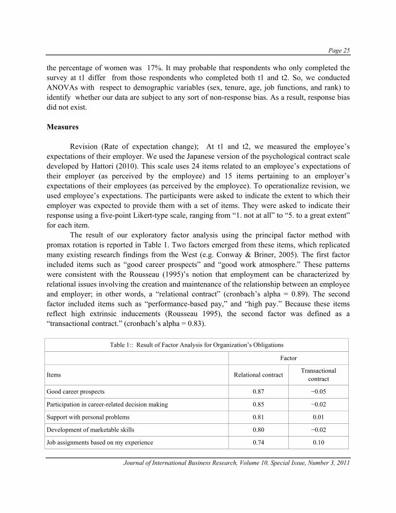
Revision (Rate of expectation change); At t1 and t2, we measured the employee’s expectations of their employer. We used the Japanese version of the psychological contract scale developed by Hattori (2010). This scale uses 24 items related to an employee’s expectations of their employer (as perceived by the employee) and 15 items pertaining to an employer’s expectations of their employees (as perceived by the employee). To operationalize revision, we used employee’s expectations. The participants were asked to indicate the extent to which their employer was expected to provide them with a set of items. They were asked to indicate their response using a five-point Likert-type scale, ranging from “1. not at all” to “5. to a great extent” for each item.
The result of our exploratory factor analysis using the principal factor method with promax rotation is reported in Table 1. Two factors emerged from these items, which replicated many existing research findings from the West (e.g. Conway & Briner, 2005). The first factor included items such as “good career prospects” and “good work atmosphere.” These patterns were consistent with the Rousseau (1995)’s notion that employment can be characterized by relational issues involving the creation and maintenance of the relationship between an employee and employer; in other words, a “relational contract” (cronbach’s alpha = 0.89). The second factor included items such as “performance-based pay,” and “high pay.” Because these items reflect high extrinsic inducements (Rousseau 1995), the second factor was defined as a “transactional contract.” (cronbach’s alpha = 0.83).
Table 1:: Result of Factor Analysis for Organization’s Obligations
Factor
Items Relational contract Transactional contract
Good career prospects 0.87 −0.05
Participation in career-related decision making 0.85 −0.02
Support with personal problems 0.81 0.01
Development of marketable skills 0.80 −0.02
Job assignments based on my experience 0.74 0.10

Page 26
Journal of International Business Research, Volume 10, Special Issue, Number 3, 2011
Table 1:: Result of Factor Analysis for Organization’s Obligations
Factor
Items Relational contract Transactional contract
Good work atmosphere 0.70 0.12
Benefits for my family 0.69 0.07
Participative decision making 0.66 0.15
Adequate job support 0.65 0.23
Adequate opportunity for OJT 0.60 0.29
Frequency of feedback 0.59 0.14
Flexibility in working hours 0.58 0.05
Interesting work 0.55 0.30
Provision of adequate training 0.50 0.31
Significant task for society 0.50 0.33
Adequate job status 0.48 0.23
Adequate allocation −0.03 0.89
Adequate difficulty of work −0.02 0.85
Performance-based pay −0.03 0.83
Meaningful tasks for me 0.19 0.68
High pay 0.18 0.63
Career development 0.28 0.47
Eigenvalue 12.36 11.10
1: Shading means factor loading above 0.4. 2: Factor correlation is 0.83
To obtain the “revision,” we divided the “expectations at t2” by the “expectations at t1.”
This resulting synthetic value is the change rate in expectations from t1 to t2. A value of 1 indicates no change, a value of greater than 1 indicates an upward revision of expectations, and a value of less than 1 indicates a downward revision of expectations.
Balancing (Rate of employees’ fulfillment change); We also measured employees’ fulfillment at t1 and t2 using the psychological contract scale mentioned above. For rate of employees’ fulfillment change, 15 items pertaining to an employer’s expectations of their employees (as perceived by the employee) were used. The participants were asked to indicate the

Page 27
Journal of International Business Research, Volume 10, Special Issue, Number 3, 2011
extent to which they fulfilled with a set of items (e.g. following instructions, long tenure of service, and association with superiors outside of work). They were asked to respond according to each item using a five-point Likert-scale ranging from “1. not at all fulfilled” to “5. totally fulfilled.” To obtain the “balancing,” we divided “fulfillment expectations at t2” by “fulfillment at t1.” The resulting synthetic value indicates the change rate of employees’ fulfillment from t1 to t2. A value of 1 indicates no change, a value of greater than 1 indicates an upward change, and a value of less than 1 indicates a downward change.
Desertion (Rate of employees’ intent to leave); Additionally, we measured employees’ intent to leave at t1 and t2. We used original items such as “I often think about quitting my job at my current organization” and “I want to stay with this organization for a long time (reverse),” which ranged from “1. strongly disagree” to “5. strongly agree.” To obtain the “desertion,” we divided “intent to leave at t2” by “intent to leave at t1.” The resulting synthetic value indicates the change rate in employees’ intent to leave the organization from t1 to t2. A value of 1 indicates no change, a value of greater than 1 indicates an upward change of intent, and a value of less than 1 indicates a downward change. Although “intent to leave” is different from actually “leaving,” it might precede such an occurrence.
Contract breach /fulfillment; In t1 and t2, we measured the employer’s fulfillment. For each item (same as expectation), participants were asked to indicate the extent to which their employers actually fulfilled. Participants were asked to respond to each item using a five-point Likert-scale, ranging from “1. not at all fulfilled” to “5. totally fulfilled.” A high score indicated high perceived fulfillment, and a low score indicated little or no fulfillment. To obtain the “contract breach/ fulfillment, we divided “fulfillment at t2” by “expectations at t1” to obtain “fulfillment weighted by t1 expectations.” The resulting synthetic value represents the rate at which the degree of fulfillment at t2 is higher than the level of expectations at t1. A value of greater than 1 indicates that an employee’s perception of an item being “fulfilled,” and a value of less than 1 indicates that their expectations were “breached.”
Career related variables; We measured other demographic and career-related variables such as employees’ sex (0=female; 1=male), employees with initial three years after job change (0=no; 1=yes), whether they were a manager (0=no; 1=yes), job function, and tenure. For job functions, organizational records were used to code the respondents’ job functions into binary codes. We coded two functions: medical representative (MR_d) and research and development (RandD_d). For the MR dummy (RandD), the MR (RandD) represents one, and others represent zero. Finally, employee with initial three years in employment was coded as 1, and all others were coded as 0.

Page 28
Journal of International Business Research, Volume 10, Special Issue, Number 3, 2011
Analytical Models
We conducted a three-step hierarchical regression analysis. Revision, balancing, and desertion were set as the dependent variables in this study. Demographics (step1), contract breach/fulfillment (step2), and the interaction term of contract breach/fulfillment × several career variables (step3) were regressed onto the three types of self-regulative changes.
RESULTS
The means, standard deviations, and inter-correlations of the study variables are presented in Table 2. The results of the hierarchical regression analysis concerned with revision are shown in Table 3. The second column from the left in Table 3 indicates a relational contract and the right column indicates a transactional contract. The results of step 3 found a significant F statistic (F=419.803, p < 0.001) with a high coefficient of determination (adjusted R2=0.607). The results of hierarchical regression analysis concerning transactional contracts are shown in the right column of Table 3. The results of step 3 found significant F statistic (F=465.252, p < 0.001) with a high coefficient of determination (adjusted R2=0.632). Hypothesis 1a predicted in case there is a discrepancy between the level of fulfillment at t2 and expectation t1, employee change the level of their expectation. In order to support this hypothesis, fulfillment weighted by t1 expectations had to have a significant impact. Table 3 shows that the fulfillment/breach of relational contracts had a significant impact on the revision (β=0.782, p<0.001). Additionally, Table 3 shows that the fulfillment/breach of transactional contracts had a significant impact on the revision (β=0.785, p<0.001). Employee’s perception of the rate of the degree of fulfillment at t2 was higher (lower) than the level of expectations at t1, which means that employees revised their expectations upward (downward). Therefore, Hypothesis 1a was supported.
The results of the hierarchical regression analysis concerning balancing are shown in Table 4. The second column from the left in Table 4 indicates a relational contract and the right column indicates a transactional contract. The results of step 3 found a significant F statistic (F=48.880, p < 0.001) with a high coefficient of determination (adjusted R2=0.150). The results of the hierarchical regression analysis concerning transactional contracts are shown in the right column in Table 4. The results of step 3 found significant F statistic (F=41.005, p < 0.001) with a high coefficient of determination (adjusted R2=0.129). Table 4 indicates that the fulfillment/breach of relational contracts had a significant impact on the balancing (β=0.278, p<0.001). Additionally, fulfillment/breach of transactional contracts had a significant impact on the revision (β=0.229, p<0.001). Therefore, Hypothesis 1b was supported.
The results of the hierarchical regression analysis concerning desertion are shown in Table 5. The second column from the left in table 5 indicates a relational contract and the right column indicates a transactional contract. The results of step 3 found a significant F statistic (F=4.795, p<0.001) with a high coefficient of determination (adjusted R2= .01). The results of

Page 29
Journal of International Business Research, Volume 10, Special Issue, Number 3, 2011
hierarchical regression analysis concerning transactional contract are shown in the right column of table 5. The results of step 3 found a significant F statistic (F=5.345 p<0.001) with a high coefficient of determination (adjusted R2= .016). Table 5 shows that the fulfillment/breach of relational had a significant impact on the desertion (β=-0.097, p<0.005). Additionally, the fulfillment/breach of transactional contracts had a significant impact on the desertion (β=-0.139, p<0.001). Therefore, Hypothesis 1c was supported.
By comparing the explanative power of each self-regulation pattern, it can be seen that the adjusted R2 of step 3 is largest in Table 3, i.e., desertion (0.607 for relational contracts and 0.632 for transactional contracts). This result indicates that the explanatory power of a gap between the level of relational/transactional contract fulfillment and expectations on revision is stronger for revision than for balancing or desertion. As to balancing, the adjusted R2 was quite low.
An examination of Tables 3, 4, and 5 shows that the interaction term of contract fulfillment/breach × initial 3year only had a significant impact on the dependent variables in Table 4, i.e., balancing (β=0.337, p<0.001 for relational; β=0.161, p<0.05 for transactional). Therefore, Hypothesis 2b was supported, but 2a and 2c were not. The interaction term of contract fulfillment/breach × employees with initial three years after job change only had a significant impact on the revision for relational contracts in Table 3 (β=0.146 p<0.001). Therefore, hypothesis 3a was supported, but 3b and 3c were not.
Table 2: Descriptive statistics for Variables Variables M SD 1 2 3 4 5 6 7 8 9 10 11
1 Sex dummy (0 = female; 1 = male)
.90 0.30 1
2 Job change dummy (0 = no; 1 = yes)
.17 0.38 .017a 1
3 MR dummy (0 = other; 1 = MR)
.64 0.48 .113a .174a 1
4 R and D dummy (0 = other; 1 = R and D)
.20 0.40 -.048a -.118a -.683a 1
5 Manager dummy (0 = other; 1 = manager)
.38 0.48 .190a -.059a .009 -.053a 1
6 Initial 3year_dummy .033 .178 -.062a .099a -.042a .065a -.076a 1
7 Revision (relational) 1.06 .279 -.031b .003b .038b -.025c .023c -.028c 1
8 Revision (transactional) 1.063 .307 -.018c .007 .022c -.022b .006 .008 .753a 1
9 Balancing 1.045 .217 -.042a -.001 -.019c .002 -.014c -.006 .385a .363a 1
10 Desertion 1.028 .402 -.028c -.039b -.021c -.029c -.026c -.043a -.40a -.06a -.100a 1
11 Fulfillment weighted by t1 expectations (relational)
.917 .268 -.021c .012c .038b -.005 .044a -.009 .774a .614a .369a -.080a 1
12 Fulfillment weighted by t1 expectations (transactional)
.913 .931 -.038b .008 .016c .001 .048a .014c .607a .792a .341a -.110a .774a
a = *** p< .01, b -** p< .05, c=* p< .10

Page 30
Journal of International Business Research, Volume 10, Special Issue, Number 3, 2011
Hierarchical regression analysis: Revision
Revision (relational) Revision (transactional)
Step1 Step2 Step3 Step1 Step2 Step3
Intercept 1.071*** .339 ** .359 *** 1.064 *** .310 *** .333 ***
Sex dummy -.042 ** -.010 -.010 -.013 .022 .022
Job change dummy .001 -.005 -.139 ** .002 -.003 -.087 **
MR dummy .027 -.004 -.003 .015 -.009 -.009
R and D dummy .007 -.017 -.016 -.002 -.025 * -.022 *
Manager dummy .018 -.006 -.006 .006 -.024 ** -.024 **
Initial 3year_dummy -.043 -.030 -.021 .017 -.006 -.085
Contract fulfillment/breach .805 ** .782 *** .810 *** .785 ***
Contract fulfillment/breach × Initial 3year_dummy
-.013 .079
Contract fulfillment/breach × Job change dummy
.146 *** .090 *
Adjusted R2 .002 .605 .607 -.002 .630 .632
R2 .004 .606 .609 .001 .631 .633
Δ R2 .602 *** .003 *** .630 ** .002 ***
F value 1.769 534.197 *** 419.803 *** .362 592.652 *** 465.252 ***
*** p< .01, ** p< .05, * p< .10
Table4: Hierarchical regression analysis: Balancing
Balancing (relational) Balancing (transactional)
Step1 Step2 Step3 Step1 Step2 Step3
Intercept 1.081 *** .804 *** .827 *** 1.081 *** .845 *** .868 ***
Sex dummy -.025 -.013 -.012 -.025 -.014 -.014
Job change dummy .001 -.001 -.077 * .001 .000 -.054
MR dummy -.015 -.026 ** -.026 ** -.015 -.022 * -.022 *
R and D dummy -.013 -.022 -.020 -.013 -.020 -.017
Manager dummy -.002 -.011 -.012 -.002 -.012 -.012
Initial 3year_dummy -.005 .000 -.307 *** -.005 -.012 -.168 **
Contract fulfillment/breach .304 *** .278 *** .254 *** .229 ***
Contract fulfillment/breach × Initial 3year_dummy
.337 *** .161 **
Contract fulfillment/breach × Job change dummy
.081 * .057
Adjusted R2 -.001 .131 .150 -.001 .123 .129
R2 .002 .144 .153 .002 .126 .132
Δ R2 .142 *** .010 *** .124 *** .006 ***
F value .694 58.327 *** 48.880 *** .694 49.833 *** 41.005 ***
*** p< .01, ** p< .05, * p< .10

Page 31
Journal of International Business Research, Volume 10, Special Issue, Number 3, 2011
DISCUSSION
Conclusion and Discussion
The purpose of this paper was to investigate employees’ self-regulative actions concerning gaps between the level of employers’ fulfillment and employees’ expectation. As discussed above, although existing studies mainly focused on the effects of contract fulfillment/breach on employees’ attitudes, we know little about the dynamic self-regulative nature of psychological contracts. The important point is that although psychological contracts can be breached frequently, which will result in employees’ negative attitudes, the contracts themselves still exist and continue to work in many cases. In this paper, we investigated the reason from the perspective of self-regulation. The results show that employees compare a level of fulfillment with a level of expectation and perform three self-regulative reactions (revision, balancing and desertion) to address discrepancies. And more, the explanative power of a gap between the levels of contract breach/fulfillment is stronger for revision than balancing or desertion. As Schalk & Roe (2007) said, employees will choose the revision option when the discrepancy is moderate; i.e. not the extreme events such as one-sided downsizing. Regarding an employer’s fulfillment level, employees may have a particular range of acceptable experience; in Rousseau’s words, there is a “zone of acceptance” (Rousseau, 1995, pp. 148-149). According to Rousseau
Table5: Hierarchical regression analysis: Desertion
Desertion (relational) Desertion (transactional)
Step1 Step2 Step3 Step1 Step2 Step3
Intercept 1.112*** 1.214*** 1.201*** 1.112*** 1.243*** 1.242***
Sex dummy -.014 -.019 -.019 -.014 -.021 -.021
Job change dummy -.037* -.036 .033 -.037* -.036 .011
MR dummy -.058** -.054* -.054** -.058** -.054** -.054**
R and D dummy -.081* -.078** -.079** -.081** -.077** -.077**
Manager dummy -.030* -.027 -.026 -.030* -.025 -.025
Initial 3year_dummy -.081* -.083* -.016 -.081* -.077* -.170
Contract fulfillment/breach -.112*** -.097** -.141*** -.139***
Contract fulfillment/breach × Initial 3year_dummy
-.072 .100
Contract fulfillment/breach × Job change dummy
-.074 -.051
Adjusted R2 .005 .011 0.01 .005 .016 .016
R2 .008 .013 .014 .008 .019 .020
Δ R2 .006*** .001** .011*** .001**
F value 3.113** 4.695*** 4.795*** 3.113** 6.729*** 5.345***
*** p< .01, ** p< .05, * p< .10

Page 32
Journal of International Business Research, Volume 10, Special Issue, Number 3, 2011
(1995), this refers to the perceived variety of behavior that an employee will accept from an employer without question. Only in case where the deviation is relatively large, employees will consider reducing their fulfillment and possibly leaving the employer. Thus, concerning the three self-regulative actions, revision was the most commonly chosen option.
The interaction term of fulfillment weighted by t1 expectations × initial 3year had a significant impact on the dependent variables, but only when applied to balancing. Additionally, the interaction term of fulfillment weighted by t1 expectations × initial three years after job change had a significant impact on the revision, but only for relational contract concerning balancing. These results indicate that employees in their initial three years in organization are more likely to engage in balancing rather than revision or desertion; on the other hand, employees with initial three years after job change are likely to choose revision. The results may reflect employees’ self-regulation skills. As Schalk & Roe (2007) says, it is natural for employees to choose revision options to address discrepancies. Revision option, however, needs some self-control skill. Employees in initial three years may have relatively poor self-control skills. Employees with job change experience, on the other hand, tend to have better developed self-control skills because they may have had self-regulative experiences in a previous organization.
Results of this paper suggest that employees who found discrepancy between their expectation and actual fulfillment by organization will feel uncomfortable, and surely conduct three types of self-regulative corrective actions. This may suggest the reason why contracts itself are still exist and work in case Japanese employer’s frequent breach. Negative effect of employer’s contract breach on employment relationship has been covered to some degree by employee’s self-regulative action (especially revision). And more, results suggest the salient role of career-related factors in predicting employee’s response to breach. Especially, the results indicate that employees in their initial three years are more likely to engage in balancing i.e. reducing their own contributions. This indicate that employer must quickly build-up fine-tuned psychological contracts with employees to minimize negative outcomes (such as reduced contribution), For example, employer can use some communication strategies such as interviews to ascertain what employees expect and are expected.
Limitations
The first limitation is our operationalization of “desertion.” As discussed above, “intent to leave” is different from actual exit. Second, the survey respondents were employees in a large and stable company. We must conduct research with other sample populations to confirm the generalizability of our results. Finally, we need more scrutiny of the employee’s choice of three self-regulative options. It is still not understood why employees with job change experience are more likely to engage in revision and employees in their initial three years of employment are more likely to engage in balancing. We must also understand the conditions that cause

Page 33
Journal of International Business Research, Volume 10, Special Issue, Number 3, 2011
employees to choose the option to desert an organization. These limitations should be addressed in future research.
REFERENCES Abegglen, J. C. (1958). The Japanese Factory: Aspects of Its Social Organization. Glencoe, Illinois: The Free Press. Adams, J. (1965). Inequity in social exchange. Advances in Experimental Social Psychology, 2, 267-299. Ashford, S. (1986). Feedback Seeking as an Individual Adaptation: A Resource Perspective for Creating
Information. Administrative Science Quarterly, 29(3), 465-487. Axelrod, R. (1984). The Evolution of Cooperation. Basic Books. Bandura, A. (1989). Self-regulation of Motivation and Action through Internal Standards and External Goal
Systems. In Pervin L. A. (eds.) Goal Concept in Personality and Social Psychology, Hillsdale, NJ: Lawrence Erlbaum.
Bandura, A. (1991). Social Cognition Theory of Self-regulation. Organizational Behavior and Human Decision Process, 50(2), 248-287.
Brief, A., and Hollenbeck, J. (1985). An exploratory study of self-regulating activities and their effects on job performance. Journal of Occupational Behavior, 6(3), 197-208.
Conway, N., and Briner, R. B. (2002). A Daily Diary Study of Affective Responses to Psychological Contract Breach and Exceeded Promises. Journal of Organizational Behavior, 23(3), 287-302.
Conway, N., and Briner, R. B. (2005). Understanding psychological contracts at work, Oxford University Press. Coyle-Shapiro, J. A-M. (2002). A Psychological Contract Perspective on Organizational Citizenship Behavior.
Journal of Organizational Behavior, 23(8), 927-946. Festinger, L. (1957). A theory of cognitive dissonance, Row, Peterson and Company. Frayne, C. (1991). Reducing employee absenteeism through self-management training: A research-based analysis
and guide. Quorum Books Westport, CT. Frayne, C., and Geringer, J. (2000). Self-management training for improving job performance: A field experiment
involving salespeople. Journal of Applied Psychology, 85(3), 361-372. Hattori, Y. (2010). Psychological Contract in Japanese Companies: An Explorative Study on Contents, Fulfillment,
and Breach of Contracts. In Bebenroth, R., and Kanai, T. (Eds.) Challenges of Human Resource Management in Japan (pp. 150-170). Routledge.
Higgins, E. T. (1987). Self-discrepancy: A theory of relating self and affect. Psychological Review, 94(3), 319-340. Homans, G. C. (1961). Social Behavior; Its elementary forms, Harcourt Brace Javanovich Inc. Kanfer, F. H., and Hagerman, S. (1987). A model of self-regulation. In Halisch, F. and Kuhl, J. (Eds.) Motivation
intention and volition (pp. 293-307). Berlin: Springer-Verlag. Katz, R. (1980). Time and Work: Toward an Integrative Perspective. Research in Organizational Behavior, 2, 81-
127. Lambert, L. S., Edwards, J. R., & Cable, D. M. (2003). Breach and Fulfillment of the Psychological Contract: A
Comparison of Traditional and Expanded Views. Personnel Psychology, 56(4), 895-934. Latham, G., and Budworth, M. (2006). The effect of training in verbal self-guidance on the self-efficacy and
performance of Native North Americans in the selection interview. Journal of Vocational Behavior, 68(3), 516-523.
Louis, M. R. (1980). Surprise and Sense Making: What Newcomers Experience in Entering Unfamiliar Organizational Setting. Administrative Science Quarterly, 25(2), 226-251.
Lyons, P. (2008). The crafting of jobs and individual differences. Journal of Business and Psychology, 23, 25-36(1).

Page 34
Journal of International Business Research, Volume 10, Special Issue, Number 3, 2011
Robinson, S. L., Kraatz, M. S., & Rousseau, D. M. (1994). Changing Obligations and the Psychological Contract: A Longitudinal Study. Academy of Management Journal, 37(1), 137-152.
Rousseau, D. M. (1989). Psychological and Implied Contracts in Organizations. Employee Responsibilities and Rights Journal, 2(2), 121-139.
Rousseau, D. M. (1995). Psychological Contracts in Organizations: Understanding Written and Unwritten Agreements, SAGE Publications, Inc.
Salancik, G. R., & Pfeffer, J. (1978). A Social Information Processing Approach to Job Attitudes and Task Design. Administrative Science Quarterly, 23(2), 224-253.
Schalk R., & Roe, E. R. (2007). Towards a Dynamic Model of the Psychological Contract. Journal of the Theory of Social Behavior, 37(2), 167-182.
Schein, E. H. (1978). Career Dynamics, Addison-Wesley Publishing Company, Inc. Thomas, H. D. & Anderson, N. (1998). Changes in Newcomer’s Psychological Contracts during Organizational
Socialization: A Study of Recruits Entering the British Army. Journal of Organizational Behavior, 19(S1), 745-767.
Wanous, J. (1976). Organizational Entry: From Naïve Expectations to Realistic Beliefs. Journal of Applied Psychology, 61(1), 22-29.
Zhao, H., Wayne, S. J., Glibkowski, B., & Bravo, J. (2007). The Impact of Psychological Contract Breach on Work-Related Outcomes: A Meta-Analysis. Personnel Psychology, 60(3), 647-680.
Zimmerman, B. J., & Schunk, D. H. (2001). Self-Regulated Learning and Academic Achievement: Theoretical Perspectives, Routledge.

Page 35
Journal of International Business Research, Volume 10, Special Issue, Number 3, 2011
A COMPARISON OF THE INTERNATIONAL FINANCIAL REPORTING STANDARDS (IFRS) AND
GENERALLY ACCEPTED ACCOUNTING PRINCIPLES (GAAP) FOR SMALL AND MEDIUM-SIZED ENTITIES
(SMES) AND COMPLIANCES OF SOME ASIAN COUNTRIES TO IFRS
Venus Ibarra, University of Guam
Martha G. Suez-Sales, University of Guam
ABSTRACT This paper compares International Financial Accounting Standards (IFRS) with Generally Accepted Accounting Principles (GAAP) for small and medium-sized entities (SMEs). It touches in part convergence by the Financial Accounting Standard board (FASB) and International Accounting Standard Board (IASB) in bringing IFRS and GAAP to become one international set of standards. Countries will adopt IFRS in response to this global convergence. Asian countries have started compliance with these standards as early as June 2003 when first time adoption was issued by London International Accounting Standards Board (IASB). This paper will present the compliance of selected Asian countries such as China, India, Indonesia, Japan, Korea, Malaysia, Philippines, Singapore, Thailand, and Vietnam with the IFRS as of 2009-2010.
INTRODUCTION Extensive preparation and emphasis has been given to the worldwide adoption of International Financial Reporting Standards (IFRS), however IFRS for small and medium-sized entities (SME) should be equally emphasized. IFRS for SMEs are modified IFRS standards tailored to third party users of small and midsize companies that have no public accountability and still need to issue financials for lending, management, and other purposes. Public accountability is applicable when an entity’s debt or equity instruments are publicly traded or the entity is a financial institution or other that, as part of its primary business, holds assets in a fiduciary capacity for a broad group of outsiders. If the assets are held in a fiduciary capacity, such as a public utility company, this will not be a cause for an entity to have public accountability. Moreover, the standards for SMEs are more user-friendly for preparers and users
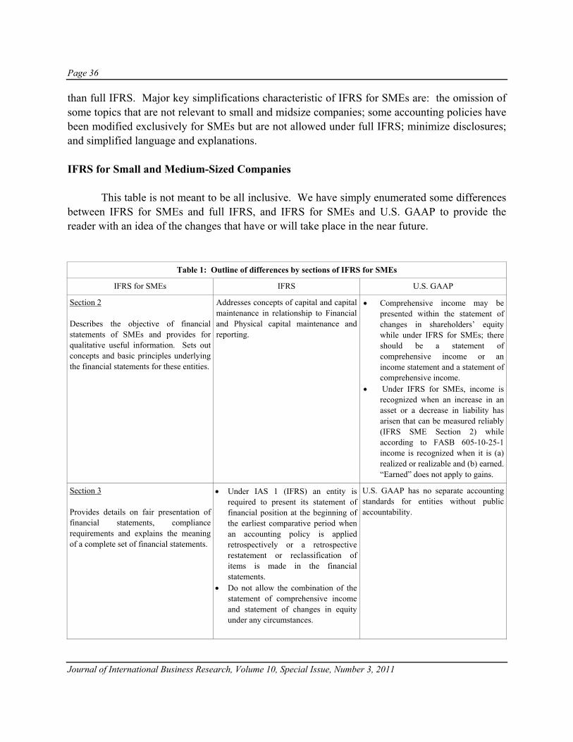
Page 36
Journal of International Business Research, Volume 10, Special Issue, Number 3, 2011
than full IFRS. Major key simplifications characteristic of IFRS for SMEs are: the omission of some topics that are not relevant to small and midsize companies; some accounting policies have been modified exclusively for SMEs but are not allowed under full IFRS; minimize disclosures; and simplified language and explanations. IFRS for Small and Medium-Sized Companies
This table is not meant to be all inclusive. We have simply enumerated some differences between IFRS for SMEs and full IFRS, and IFRS for SMEs and U.S. GAAP to provide the reader with an idea of the changes that have or will take place in the near future.
Table 1: Outline of differences by sections of IFRS for SMEs
IFRS for SMEs IFRS U.S. GAAP
Section 2 Describes the objective of financial statements of SMEs and provides for qualitative useful information. Sets out concepts and basic principles underlying the financial statements for these entities.
Addresses concepts of capital and capital maintenance in relationship to Financial and Physical capital maintenance and reporting.
• Comprehensive income may be presented within the statement of changes in shareholders’ equity while under IFRS for SMEs; there should be a statement of comprehensive income or an income statement and a statement of comprehensive income.
• Under IFRS for SMEs, income is recognized when an increase in an asset or a decrease in liability has arisen that can be measured reliably (IFRS SME Section 2) while according to FASB 605-10-25-1 income is recognized when it is (a) realized or realizable and (b) earned. “Earned” does not apply to gains.
Section 3 Provides details on fair presentation of financial statements, compliance requirements and explains the meaning of a complete set of financial statements.
• Under IAS 1 (IFRS) an entity is required to present its statement of financial position at the beginning of the earliest comparative period when an accounting policy is applied retrospectively or a retrospective restatement or reclassification of items is made in the financial statements.
• Do not allow the combination of the statement of comprehensive income and statement of changes in equity under any circumstances.
U.S. GAAP has no separate accounting standards for entities without public accountability.

Page 37
Journal of International Business Research, Volume 10, Special Issue, Number 3, 2011
Table 1: Outline of differences by sections of IFRS for SMEs
IFRS for SMEs IFRS U.S. GAAP
Section 4 Provides guidance regarding information presented in the statement of financial position.
IAS 1 (IFRS) requires separate presentation of assets classified as held for sale and assets and liabilities included in disposal groups also classified as held for sale in accordance with IFRS 5, no such a distinction is made under IFRS for SMEs.
There are no major differences under U.S. GAAP.
Section 5 It requires an entity to present its comprehensive income in one or two financial statements. It provides guidance regarding presentation.
IFRS IAS 1 includes gains and losses arising from the derecognition of financial assets measured at amortized cost, and if a financial asset is reclassified so that it is measured at fair value, any gain or loss arising from a difference between the previous carrying amount and its fair value at the reclassification date is also included (as defined in IFRS 9) in addition to the minimum line items required under Section 5 of IFRS for SMEs.
• FASB 220-10-55-2 items e – g which deals with unrealized gains and losses on available-for-sale securities are excluded from other comprehensive income under IFRS for SMEs.
• The presentation of certain items as extraordinary is required. However, IFRS for SMEs section 5 prohibits disclosure of any item of income and expense as “extraordinary items”.
Section 6 Provides the requirements for the presentation of changes in an entity’s equity for a period.
Do not allow the statement of changes in equity to be combined with the statement of comprehensive income
A separate statement of changes in equity is not required.
Section 7 It provides reporting guidance for the statement of cash flows.
• AIS 2 for full IFRS provides for certain conditions when cash flows are allowed to be reported net.
• Additionally, full IFRS encourages the direct method when reporting cash flows from operating activities.
Under FASB 230-10-45-9, U.S. GAAP permits netting of cash receipts when the original maturity of the asset or liability is three months or less and it pertains to investments (other than cash equivalents), loans receivable, or debt.
Section 9 Provides for guidance and procedures for presentation of consolidated financial statements.
IAS 27 (IFRS) allows a maximum of three months for differences in group reporting dates, and it includes guidance on the adjustments required when there is a difference.
• Additionally, when a parent loses control over a subsidiary but continues to hold an investment in the former subsidiary, under full IFRS, the former subsidiary’s assets and liabilities and any non-controlling interest in the subsidiary is derecognized at their carrying amount. A continuing investment in the former subsidiary is initially measured at fair value. Any
• In terms of a uniform reporting date, U.S. GAAP provides that a parent may elect to use a date of no more than three months from its reporting date for a subsidiary but has to demonstrate that it is unfeasible to use the parent’s reporting date.
• Another important difference rests on the requirement of consolidated financial statements. U.S. GAAP requires all majority-owned subsidiaries to be consolidated except when the subsidiary is in legal reorganization, the subsidiary is in bankruptcy, the subsidiary operates under foreign exchange

Page 38
Journal of International Business Research, Volume 10, Special Issue, Number 3, 2011
Table 1: Outline of differences by sections of IFRS for SMEs
IFRS for SMEs IFRS U.S. GAAP
resulting difference is recognized as a gain or loss attributable to the parent (IFRS IAS 27).
• Furthermore, IFRS for SMEs section 9 provides that on disposal of a foreign subsidiary, foreign exchange differences recognized in equity are not recycled to profit or loss as it is the case under full IFRS as prescribed by IAS 27.
restrictions, controls, or other governmentally imposed uncertainties so severe that they cast significant doubt on the parent’s ability to control the subsidiary, or the powers of a shareholder with a majority voting interest to control the operations or assets of the investee are restricted by a noncontrolling shareholder that is granted approval or veto rights (FASB 810-10-15).
• Also, losses that exceed the minority interest in the equity of a subsidiary may create a debit balance in minority interests only if the minority has a requirement to subsidize and can make an additional investment to cover the losses; otherwise, the losses are attributed to the parent.
Section 11 Deals with basic financial instruments and is relevant to all entities unlike the next section which provides guidance for more complex financial instruments and transactions.
• IFRS 9 for full IFRS permits the designation of financial instruments at fair value through profit or loss (fair value option).
• Under IAS 39 (IFRS), reversal of impairment losses on equity instruments is not permitted.
• Under Section 11, of IFRS for SMEs, financial assets are derecognized when: the contractual rights to the cash flows expire or are settled; substantially all the risks and rewards of ownership have been transferred; or despite retaining some risks and rewards, control of the financial asset has been transferred and the other party has a practical ability to sell the asset in its entirety without needing to impose additional restrictions on the transfer. IAS 39 for full IFRS, contains in addition to the items listed the need to assess pass-through arrangements and whether there is continuing involvement.
• Under U.S. GAAP, there is no distinguishment for basic financial instruments from other financial instruments.
• According to Section 11, debt instruments that meet the conditions of paragraph 11.8(b) are measured at amortized cost using the effective interest method. While under U.S. GAAP, certain loans classified as held-for-sale are measured at lower-of-cost-or-market in accordance with FAS 65, debt securities classified as trading or available for sale are reported at fair value (SFAS 115), and under the fair value option, an entity has an option to measure most financial assets and liabilities at fair value.
• Unlike IFRS for SMEs, reversal of impairment write-downs is not allowed under U.S. GAAP.

Page 39
Journal of International Business Research, Volume 10, Special Issue, Number 3, 2011
Table 1: Outline of differences by sections of IFRS for SMEs
IFRS for SMEs IFRS U.S. GAAP
Section 12 Applies to complex financial instruments and transactions not within the scope of Section 11. It does not apply to interests in subsidiaries, associates or joint ventures, employers’ rights and obligations under employee benefit plans, an entity’s own equity, or contracts for contingent consideration in a business combination (acquirer only).
• In addition to the hedge accounting risks allowed under Section 12, IAS 39 under full IFRS allows more risks for hedging and hedging of the entire hedged item is permitted. A single hedging instrument may be designated as a hedge of multiple risks.
• Furthermore, under full IFRS, hedge accounting for portfolios is permitted.
• Under Section 12, hedge accounting can only be applied if the hedge is expected to be highly effective at inception and at the beginning of each financial year (prospective test) but no specific effectiveness threshold is included and no retrospective effectiveness test is required, while IAS 39 (IFRS) includes an 80% - 125% threshold for a hedge to be highly effective and retrospective hedge effectiveness testing is required.
• Section 12 provides for the conditions that must be met in order to qualify for hedge accounting these are less restrictive than U.S. GAAP. FASB 815-20-25 requires strict documentation, effectiveness testing, and other requirements to qualify.
• Unlike IFRS for SMEs, hedge accounting for portfolios is permitted under U.S. GAAP.
Section 13 Applies to all inventories except for work in process arising from construction contracts, financial instruments, and biological assets and agricultural produce at the point of harvest.
• This section prescribes for measurement of inventories at the lower of cost and estimated selling price less costs to complete and sell while IAS 2 under full IFRS requires inventory to be measured at lower of cost and net realizable value. Net realizable value is defined as estimated selling price less the estimated costs of selling and the estimated costs to make the sale.
• IAS 23 provides guidance when in certain circumstances under full IFRS; borrowing costs are included in the cost of inventory.
• FASB 330-10-35 states that inventory is to be measured at the lower of cost or market. The term market means current replacement cost not to exceed a ceiling of net realizable value (selling price less reasonably estimable costs of completion and disposal) or be less than a floor of net realizable value adjusted for a normal profit margin (Epstein, Bragg & Nach, 2010).
• Under certain circumstances, exceptions for reflecting assets at selling prices are permissible when dealing with inventories of gold and silver as well as agricultural, mineral, and other products that meet the criteria of FASB 330-10-35-16.
• Under U.S. GAAP, a variety of inventory costing methodologies are permitted including LIFO (last-in-first-out) which is not allowed under either full IFRS or IFRS for SMEs.
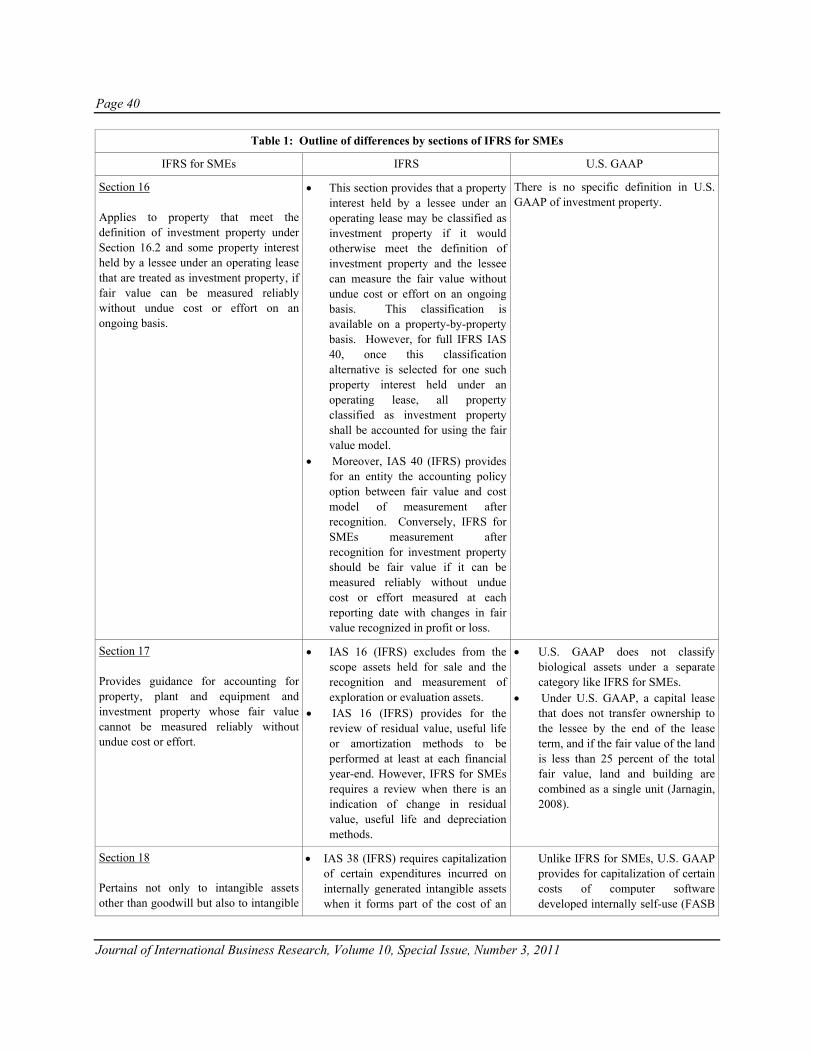
Page 40
Journal of International Business Research, Volume 10, Special Issue, Number 3, 2011
Table 1: Outline of differences by sections of IFRS for SMEs
IFRS for SMEs IFRS U.S. GAAP
Section 16 Applies to property that meet the definition of investment property under Section 16.2 and some property interest held by a lessee under an operating lease that are treated as investment property, if fair value can be measured reliably without undue cost or effort on an ongoing basis.
• This section provides that a property interest held by a lessee under an operating lease may be classified as investment property if it would otherwise meet the definition of investment property and the lessee can measure the fair value without undue cost or effort on an ongoing basis. This classification is available on a property-by-property basis. However, for full IFRS IAS 40, once this classification alternative is selected for one such property interest held under an operating lease, all property classified as investment property shall be accounted for using the fair value model.
• Moreover, IAS 40 (IFRS) provides for an entity the accounting policy option between fair value and cost model of measurement after recognition. Conversely, IFRS for SMEs measurement after recognition for investment property should be fair value if it can be measured reliably without undue cost or effort measured at each reporting date with changes in fair value recognized in profit or loss.
There is no specific definition in U.S. GAAP of investment property.
Section 17 Provides guidance for accounting for property, plant and equipment and investment property whose fair value cannot be measured reliably without undue cost or effort.
• IAS 16 (IFRS) excludes from the scope assets held for sale and the recognition and measurement of exploration or evaluation assets.
• IAS 16 (IFRS) provides for the review of residual value, useful life or amortization methods to be performed at least at each financial year-end. However, IFRS for SMEs requires a review when there is an indication of change in residual value, useful life and depreciation methods.
• U.S. GAAP does not classify biological assets under a separate category like IFRS for SMEs.
• Under U.S. GAAP, a capital lease that does not transfer ownership to the lessee by the end of the lease term, and if the fair value of the land is less than 25 percent of the total fair value, land and building are combined as a single unit (Jarnagin, 2008).
Section 18 Pertains not only to intangible assets other than goodwill but also to intangible
• IAS 38 (IFRS) requires capitalization of certain expenditures incurred on internally generated intangible assets when it forms part of the cost of an
Unlike IFRS for SMEs, U.S. GAAP provides for capitalization of certain costs of computer software developed internally self-use (FASB

Page 41
Journal of International Business Research, Volume 10, Special Issue, Number 3, 2011
Table 1: Outline of differences by sections of IFRS for SMEs
IFRS for SMEs IFRS U.S. GAAP
assets held by an entity for sale in the ordinary course of business.
intangible asset that meets the recognition criteria (paragraphs 18–67); or when the item is acquired in a business combination and cannot be recognized as an intangible asset. If this is the case, it forms part of the amount recognized as goodwill at the acquisition date (IFRS 3). However, Section 18 for IFRS for SMEs requires expenditures incurred on internally generated items to be recognized as an expense when incurred unless it forms part of the cost of another asset that meets the recognition criteria of this section.
• Additionally, in accordance with IAS 23 (IFRS), borrowing costs directly attributable to the production of an intangible asset must be capitalized as part of its cost.
• IFRS for SMEs differs from full IFRS when considering all intangible assets to have a finite useful life while IAS 38 for full IFRS makes a distinction between indefinite and finite useful life for intangibles.
• Section 18 requires amortization period and method to be reviewed when there is an indication that they have changed since the prior reporting date while IAS 38 requires an annual review of residual value, useful life and amortization methods.
350-40-25). Under U.S. GAAP, acquired intangibles are measured initially at fair value, but under Section 18 intangibles are initially measured at cost. U.S. GAAP considers some intangible assets to have indefinite useful lives when there is no foreseeable limit on the period of time over which the intangible is expected to contribute to the cash flows of the reporting entity. Intangibles with indefinite lives are subject to annual review for impairment (FASB 350-30-35).
Section 19 Provides guidance on accounting for business combinations and goodwill both at the time of the business combination and subsequently.
Section 19 requires business combinations to be accounted for using the purchase method while IFRS 3 for full IFRS for business combinations requires the use of the acquisition method based on the fair value of the consideration transferred. Section 19 requires the inclusion of contingent consideration in the cost if it is probable and can be measured reliably. Subsequent adjustments to
Under U.S. GAAP, the acquirer recognizes the contingent consideration at acquisition-date fair value as part of the consideration transferred in exchange for the acquiree, but under Section 19, the acquirer includes any contingent consideration at the acquisition date if the adjustment is probable and can be measured reliably. This condition is not mentioned under U.S. GAAP (FASB 805-30-25).

Page 42
Journal of International Business Research, Volume 10, Special Issue, Number 3, 2011
Table 1: Outline of differences by sections of IFRS for SMEs
IFRS for SMEs IFRS U.S. GAAP
the estimate are recognized against goodwill. However, IFRS 3 requires contingent consideration to be recognized initially at fair value regardless of probability and any subsequent adjustments are recognized in profit or loss or other comprehensive income. Under IFRS for SMEs, Goodwill is measured at cost less accumulated amortization and impairment losses. If a reliable estimate of the useful life of goodwill cannot be made, it is presumed to be 10 years. Conversely, under full IFRS, goodwill is not amortized but tested for impairment annually.
Under Section 19, goodwill is recognized as an asset when acquired in a business combination and it is initially measured at cost (excess of cost of the business combination over the acquirer’s interest in the net fair value of the identifiable assets, liabilities and contingent liabilities). U.S. GAAP requires when measuring goodwill to also include the fair value of any noncontrolling interest in the acquiree (FASB 805-30-30).
• In accordance with FAS 142 for U.S. GAAP, goodwill is not amortized, but tested annually for impairment unlike IFRS for SMEs where goodwill is amortized over ten years.
Section 20 Applies to all leases including special arrangements that do not take legal form of a lease but convey rights to use assets in return for payments.
The scope as described under IAS 17 (IFRS) does not exclude onerous operating leases and other leases in the scope of Section 12 as IFRS for SMEs. Under Section 20, operating leases are recognized as an expense on a straight-line basis over the lease term, unless the payments are structured to increase with expected general inflation to compensate for the lessor’s expected inflationary cost increases or another systematic basis is more representative of the pattern of benefit. But, under full IFRS IAS 17 and SIC 15, there is no such an exclusion of recognition.
• This section covers measurement of property held by lessees that are accounted for as investment property, but there is no such a concept under U.S. GAAP.
• U.S. GAAP does not exclude from its scope operating leases that are onerous as IFRS for SMEs does.
• Under U.S. GAAP the concepts to determine if a lease is a capital lease to a lessee are similar to IFRS for SMEs except that U.S. GAAP in accordance with SFAS 13 provides for specific criteria that must be met in order to classify a lease as a capital lease.
• U.S. GAAP requires a lessor to classify a capital lease as either sales-type, direct financing, or leveraged.
• Under SFAS 13, a lessee calculates the present value of minimum lease payments using the lower of the interest rate implicit in the lease, if it is practicable for the lessee to learn the rate computed by the lessor, or the lessee’s incremental borrowing rate, but for

Page 43
Journal of International Business Research, Volume 10, Special Issue, Number 3, 2011
Table 1: Outline of differences by sections of IFRS for SMEs
IFRS for SMEs IFRS U.S. GAAP
IFRS for SMEs the present value of the minimum lease payments should be calculated using the interest rate implicit in the lease and if it cannot be determined then use the lessee’s incremental borrowing rate.
Section 21 Provides guidance regarding all provisions, contingent liabilities and contingent assets, except those covered by other sections such as leases, employee benefits and income tax.
Full IFRS IAS 37 provides significantly more guidance on provisions related to restructuring than what is required under this section of IFRS for SMEs.
For U.S. GAAP, the probability threshold for recognition of contingent liabilities is believed to be higher than IFRS for SMEs and although U.S. GAAP does not ascribe a threshold for “probable”, generally in practice, the threshold used is approximately 80% (Stickney, Weil, Schipper & Francis, 2007). Another difference is when measuring contingencies when there is a continuous range of possible outcomes and each point in the range is as likely as any other to occur, under U.S. GAAP (FASB Interpretation No. 14), the minimum amount in the range is used to measure the provision while under IFRS for SMEs, the midpoint of the range is used.
Section 23 Applies to the accounting for revenue arising from the sale of goods, rendering of services, construction contracts and the use by other of entity assets yielding interest, royalties or dividends. It does not apply to revenue of income arising from transactions and events dealt with in other sections of IFRS for SMEs.
IAS 18 (IFRS) excludes from the scope revenue arising from extraction of mineral ores and changes in the value of current assets, but these are not excluded under Section 23.
• Under FASB Codification 845, an exchange of a product or property held for sale in the ordinary course of business for a product or property to be sold in the same line of business to facilitate sales to customers other than the parties to the exchange are recorded based on the carrying amount of the assets given up.
• Under FASB 605-20-25, revenue from services such as warranty or product maintenance contracts are recognized using the proportional performance or straight-line method rather than the percentage-of-completion as required under Section 23.

Page 44
Journal of International Business Research, Volume 10, Special Issue, Number 3, 2011
Table 1: Outline of differences by sections of IFRS for SMEs
IFRS for SMEs IFRS U.S. GAAP
Section 27 Applies to the impairment of all assets except for deferred tax assets; assets arising from employee benefits; financial assets within Sections 11 or 12; investment property measured at fair value; and biological assets measured at fair value less estimated costs to complete.
• IAS 36 (IFRS) prescribes that intangible assets not yet available for use, those with an indefinite useful life and goodwill are tested annually for impairment.
• Additionally, grouping of cash-generating units for impairment testing of goodwill cannot result in a grouping being larger than an operating segment. This provision is not applicable under IFRS for SMEs.
• Unlike IFRS for SMEs which requires an entity to reduce the carrying amount of the asset to its recoverable amount if the recoverable amount of an asset is less than its carrying amount. U.S. GAAP under FASB 144 requires an impairment loss for intangible assets that are subject to amortization to be recognized if the carrying amount of an intangible asset is not recoverable and its carrying amount exceeds its fair value. For intangible assets that are not subject to amortization and for goodwill, impairment is recognized if the carrying amount of the asset exceeds its fair value, and for goodwill its implied fair value.
Section 28 Provides guidance to all forms of consideration given by an entity in exchange for service rendered by employees such as short-term benefits; post-employment benefits; other long-term benefits; and termination benefits.
The major differences between IFRS for SMEs and full IFRS originate from defined benefit plans: • IAS 19 (IFRS) for defined benefit
plans includes an accounting policy choice for actuarial gains or losses below a specified threshold to be deferred, and those in excess of a specified threshold to be amortized over the expected remaining working lives of employees. Section 28 for SMEs requires actuarial gains and losses from defined benefit plans to be recognized either in profit or loss or in other comprehensive income.
• Additionally, IAS 19 (IFRS) requires past service cost to be recognized as an expense over the average period until the benefits vest. However, this section requires all past service costs to be recognized immediately in profit or loss. The amount recognized for defined benefit liability includes unrecognized actuarial gains or losses and past service costs under
As prescribed by FASB 158, GAAP has four types of termination benefits: ongoing benefit arrangements, contractual terminations, special terminations and one-time terminations which are not mentioned under Section 28.
• Under U.S. GAAP, postemployment plans are not required to be classified as defined contribution plans, but they are accounted for based on the type of benefit (FAS 112, EITF Issue 05-5).
• Actuarial gains and losses arising during a period but not included as a component of net periodic benefit cost of that period should be recognized as increases or decreases in other comprehensive income. Gains and losses initially recognized in other comprehensive income should be adjusted as they are subsequently recognized as a component of net periodic benefit cost based on the applicable recognition or amortization requirements of Statement 87, 88, or

Page 45
Journal of International Business Research, Volume 10, Special Issue, Number 3, 2011
Table 1: Outline of differences by sections of IFRS for SMEs
IFRS for SMEs IFRS U.S. GAAP
IAS 19, but under IFRS for SMEs defined benefit liability is recognized as the net total of the present value obligations under the plans minus the fair value of the plan assets at the reporting date.
106 (FASB 158), however, under IFRS for SMEs, an entity can either recognize all actuarial gains and losses in the period in which they occur in profit or loss, or in the other comprehensive income. Unlike U.S. GAAP, amount recognized in OCI are not recycled to profit or loss.
Section 29 Includes all domestic and foreign taxes that are based on taxable profit and withholding taxes that are payable by a subsidiary, associate or joint venture on distributions to the reporting entity.
• Under IAS 12 (IFRS), there is no exemption from the recognition of deferred tax in respect to an asset or liability where it is not expected to have an effect on taxable profit when the entity recovers or settles its carrying amount as there is under Section 29.
• Unlike Section 29, IAS 12 requires the tax basis of assets and liabilities to be determined based on the manner of expected recovery or settlement of the carrying amount of the asset or liability.
• Deferred tax assets are only recognized to the extent that it is probable that future taxable profits will be sufficient to recover the carrying amount of the deferred tax asset. Furthermore, the use of a valuation allowance is not required but the amount of the net asset will be the same (IAS 12).
• U.S. GAAP does not address accounting for withholding taxes on dividends to shareholders (FASB 740).
• Under FASB 740-10-30, the measurement of current and deferred tax liability and assets is based on provision of the enacted law. The effects of future changes in tax law or rates are not anticipated, but under this section, an entity measures current tax liability or asset at the amounts it expects to pay or recover using the tax rates and laws that have been enacted or substantively enacted by the reporting date.
• Unlike Section 29, deferred tax is classified as either current or noncurrent based on the classification of the related asset or liability giving rise to the temporary difference.
Section 30 Provides guidance for foreign currency transactions and foreign operations, prescribes the translation of financial statements into a presentation currency, and notes that the requirements in Section 11 and 12 apply to financial instruments denominated in a foreign currency and hedge accounting of foreign currency items.
IAS 21 under full IFRS requires an entity reporting consolidating financial statements to recognized exchange differences in other comprehensive income that arose from monetary items treated as part of the net investment in a foreign operation to be recycled to profit or loss on disposal of the foreign operation unlike this section which does not permit for these exchange differences on disposal of the net investment to be reclassified to profit or loss.
• Unlike IFRS for SMEs, FASB 830-10-10 requires to translate into a single reporting currency those assets, liabilities, revenues, expenses, gains and losses that are measured or denominated in a foreign currency.
• U.S. GAAP does not prioritize the factors listed under this section more than any other factors an entity should considered in determining its functional currency

Page 46
Journal of International Business Research, Volume 10, Special Issue, Number 3, 2011
Table 1: Outline of differences by sections of IFRS for SMEs
IFRS for SMEs IFRS U.S. GAAP
Section 31 Concerns the financial statements of an entity whose functional currency is that of a hyperinflationary economy.
No key differences were identified when compared to full IFRS IAS 29.
Under U.S. GAAP, there is no requirement for an entity whose functional currency is the currency of a hyperinflationary economy to adjust its financial statements for the effects of hyperinflation.
China’s Compliance with IFRS
China is a Communist party-led state that has executive, legislative, and a judicial branch, China has different political and legal system compared to other countries. Though the Chinese Communist Party was formed in 1921, it subsequently led to the formation of the People’s Republic of China (PRC) in 1949. Since then China adopted socialism as its political system. With the founding of the PRC, resources that are essential to production in the country became state owned and thus creating state-owned enterprises, also called SOE.
In 1993, China had worked closely with Deloitte Touche Tohmatsu as a consultant to develop the Chinese Accounting Standards that would generally be in line with international accounting and financial reporting practices. About 30 exposure drafts of the standards had been published between 1994 and 1996. By the year 2000, Deloitte Touche Tohmatsu was reappointed as a consultant for the second half of the project. The remaining work was to incorporate in the CAS additional 17 standards that dealt with issues that the International Accounting Standards Committee had addressed. While in 2001, the Ministry of Finance (MOF) issued a new comprehensive “Accounting System for Business Enterprises” known as the “System”. The new system replaced both the Accounting System for Joint-Stock Limited Enterprises and Accounting Regulations for Foreign Investment Enterprises, requiring all enterprises to follow the new unified system. When the system was fully implemented, many of the regulations of the past were replaced giving way to comparability among enterprises.
The Ministry of Finance greatly supports harmonization and convergence with IFRS by drafting each China Accounting Standard in reference to IFRS. However, these standards must conform to the country’s natural laws which might cause differences between China Accounting System (CAS) and IFRS. It is interesting to note that even if significant portion of the economy is dominated by state-owned enterprises and that these enterprises go through restructuring to a more free market enterprise, many of the stakeholders are part of functional or regional government that still possess great influence in making the standards. The standards are known as PRC-GAAPs. As of 2002, there were 16 CAS that were already implemented with applicability to certain enterprises as seen in the table below:

Page 47
Journal of International Business Research, Volume 10, Special Issue, Number 3, 2011
Table 2 : CAS Implementation to Enterprises
No. Accounting Standard Effective Date Applicability
1 Disclosure of Related Party Relationships and Transactions 1 Jan. 1997 Listed Enterprises
2 Cash Flow Statements (minor revisions in 2001) 1 Jan. 2001 All Enterprises
3 Events Occuring after the Balance Sheet Date 1 Jan. 1998 Listed Enterprises
4 Debt Restructuring (revised significantly in 2001) 1 Jan. 2001 All Enterprises
5 Revenue 1 Jan. 1999 Listed Enterprises
6 Investments (minor revision in 2001) 1 Jan. 2001 Joint Stock Limted Enterprises
7 Construction Contracts 1 Jan. 1999 Listed Enterprises
8 Changes in Accounting Policies and Estimates and Corrections of Accounting Measures (minor revision in 2001)
1 Jan. 2001 All Enterprises
9 Non-monetary Transactions (revised significantly in 2001) 1 Jan. 2001 All Enterprises
10 Contingencies 1 Jul. 2000 All Enterprises
11 Intagible assets 1 Jan. 2001 Joint Stock Limted Enterprises
12 Borrowing Costs 1 Jan. 2001 All Enterprises
13 Leases 1 Jan. 2001 All Enterprises
14 Interim Financial Reporting 1 Jan. 2002 Listed Enterprises
15 Inventories 1 Jan. 2002 Joint Stock Limted Enterprises
16 Fixed Assets 1 Jan. 2002 Joint Stock Limted Enterprises
China is committed to adapt IFRS. However, there is no exact date for China’s full
implementation of its new PRC-GAAPs. China considers convergence as a huge step for the development of the Chinese economy and its position in the world’s ever increasing and developing capital markets. The new PRC-GAAPs can greatly encourage and enable investors to increase confidence in China’s capital markets.

Page 48
Journal of International Business Research, Volume 10, Special Issue, Number 3, 2011
India’s Compliance with IFRS India has the world’s 12th largest economy and the third largest in Asia after Japan and China, with a total GDP of around $1.21B based on the 2008 census. India has a “federal republic” form of government, which includes the executive branch, legislative branch, and judicial branch.
In this country, the Statements on Accounting Standards are issued by the Institute of Chartered Accountants of India (ICAI). The institute has established standards that need to be complied to ensure that financial statements are prepared in accordance with India’s Generally Accepted Accounting Standards (India’s GAAP).
In 2004, World Bank notes that considerable efforts have been made to align Indian Accounting Standards (IAS) with the International Financial Reporting Standards (IFRS). The gap between Indian and international standards has been narrowing and is likely to reach full convergence in 2011 when IFRSs are expected to be adopted in India for listed and other public interest entities. As of 2010, India has complied with the following IFRS:
IFRS 1: First-time Adoption of International Financial Reporting Standards (effective 2010) IFRS 2: Share-based Payment (effective 2010) IFRS 3: Business Combinations (effective 2010) IFRS 4: Insurance Contracts (effective 2006) IFRS 5: Non-current Assets Held for Sale and Discontinued Operations (effective 2010) IFRS 6: Exploration for and Evaluation of Mineral Resources (effective 2006) IFRS 7: Financial Instruments: Disclosures (effective 2009) IFRS 8: Operating Segments (effective 2010) IAS 1: Presentation of Financial Statements (effective 2010) IAS 2: Inventories (effective 2005) IAS 7: Cash Flow Statements (effective 2010) IAS 8: Accounting Policies, Changes in Accounting Estimates and Errors (effective 2005) IAS 10: Events after the Reporting Period (effective 2005) IAS 11: Construction Contracts (effective 1995) IAS 12: Income Taxes (effective 2001) IAS 16: Property, Plant and Equipment (revised 2009) IAS 17: Leases (effective 2010) IAS 18: Revenue (effective 1995) IAS 19: Employee Benefits (revised 2009) IAS 20: Accounting for Government Grants and Disclosure of Government IAS 21: The Effects of Changes in Foreign Exchange Rates (effective 2005) IAS 23: Borrowing Costs (revised 2009) IAS 24: Related Party Disclosures (effective 2005) IAS 26: Accounting and Reporting by Retirement Benefit Plans (effective 1998) IAS 27: Consolidated and Separate Financial Statements (effective 2010)

Page 49
Journal of International Business Research, Volume 10, Special Issue, Number 3, 2011
IAS 28: Investments in Associates (revised 2009) IAS 29: Financial Reporting in Hyperinflationary Economies (revised 2009) IAS 31: Interests in Joint Ventures (revised 2009) IAS 32: Financial Instruments: Disclosure and Presentation (effective 2010) IAS 33: Earnings per Share (effective 2005) IAS 34: Interim Financial Reporting (effective 1999) IAS 36: Impairment of Assets (revised 2009) IAS 37: Provisions, Contingent Liabilities and Contingent Assets (effective 1999) IAS 38: Intangible Assets (effective 2010) IAS 39: Financial Instruments: Recognition and Measurement (effective 2010) IAS 40: Investment Property (effective 2009) IAS 41: Agriculture (effective 2009) India has agreed to converge its accounting practices to International Financial Reporting Standards by 2011. Overall, the Indian authorities seem proactively pursuing better compliance with international standards. Compliance with the IFRS will make multiple benefits to the Indian companies especially those that intend to go global. Adapting to IFRS will enable Indian companies to have access to international capital markets and will reduce the cost of raising capital from foreign markets. Indonesia’s Compliance with IFRS
Indonesia can be classified as a developing market economy with strong influence from the government. Numerous state-owned businesses are managed by its government (Economy Watch).
The Indonesian Institute of Accountants (Ikatan Akutan Indonesia or IAI) is the only accounting body in Indonesia acknowledged by the Ministry of Finance. The IAI is also a founder of the ASEAN Federation of Accountants (Republic of Indonesia: ROSC Accounting and Auditing, 2005). Moreover, the IAI is a full member of the International Federation of Accountants (IFAC) which is a worldwide organization that aims to strengthen the accountancy profession and further the international convergence of accounting standards (Choi & Meek, 2008). The functions and powers of the IAI include setting up a code of ethics, accounting and auditing standards, conducting examinations for certified public accountants (CPA), and running programs for professional education. (Republic of Indonesia: ROSC Accounting and Auditing, 2005).
In the past decades, Indonesia’s accounting standards were based on the US GAAP. However, the IAI eventually endorsed IFRS for preparing financial reports. On December 23, 2008, the IAI has issued a formal statement and announced its plan to fully join the IFRS starting January 1, 2012 (IAI, 2009). Table 3 shows the roadmap of key events regarding the transition to IFRS:

Page 50
Journal of International Business Research, Volume 10, Special Issue, Number 3, 2011
Table 3: Key Events to IFRS from Adoption to Implementation Phase
Adoption Phase (2008-2010) Preparation (2011) Implementation (2012)
Adopt IFRS per January 1, 2009 into PSAK (Pernyataan Standar Akuntansi Keuangan or Statements of Financial Accounting Standards)
Finalization of infrastructures Implementation of new PSAK
Prepare all related infrastructures
Implementation of new PSAK Evaluate the impact of implementation of new PSAK comprehensively
Evaluate the impact of IFRS adoption to current applied PSAK
As of 2009, the following IFRS principles were implemented in Indonesia (Indonesia:
IFRS 2009). IFRS 1: First-time Adoption of International Financial Reporting Standards IFRS 2: Share-based Payment IFRS 3: Business Combinations IFRS 4: Insurance Contracts IFRS 5: Non-current Assets Held for Sale and Discontinued Operations IFRS 6: Exploration for and Evaluation of Mineral Resources IFRS 7: Financial Instruments: Disclosures IFRS 8: Operating Segments IAS 1: Presentation of Financial Statements IAS 2: Inventories IAS 7: Cash Flow Statements IAS 8: Accounting Policies, Changes in Accounting Estimates and Errors IAS 10: Events after the Reporting Period IAS 11: Construction Contracts IAS 12: Income Taxes IAS 16: Property, Plant and Equipment IAS 17: Leases IAS 18: Revenue IAS 19: Employee Benefits IAS 20: Accounting for Government Grants and Disclosure of Government Assistance IAS 21: The Effects of Changes in Foreign Exchange Rates IAS 23: Borrowing Costs IAS 24: Related Party Disclosures IAS 26: Accounting and Reporting by Retirement Benefit Plans IAS 27: Consolidated and Separate Financial Statements IAS 28: Investments in Associates

Page 51
Journal of International Business Research, Volume 10, Special Issue, Number 3, 2011
IAS 29: Financial Reporting in Hyperinflationary Economies IAS 31: Interests in Joint Ventures IAS 32: Financial Instruments: Disclosure and Presentation IAS 33: Earnings per Share IAS 34: Interim Financial Reporting IAS 36: Impairment of Assets IAS 37: Provisions, Contingent Liabilities and Contingent Assets IAS 38: Intangible Assets IAS 39: Financial Instruments: Recognition and Measurement IAS 40: Investment Property IAS 41: Agriculture Full compliance with IFRS is one of the major goals of countries throughout the world today and Indonesia is no different. Although Indonesia will be a year behind other countries in terms of converging, it will still have an advantage such as learning from those countries that have fully converged. Furthermore, Indonesia’s compliance with IFRS may create more opportunities for Indonesian companies to be recognized internationally. In 2009, the Indonesia Financial Accounting Standards Board issued accounting standards for entities without public accountability based on IFRS for SMEs with some modifications which are going to be effective for annual periods beginning on or after January 1, 2011 (PricewaterhouseCoopers, 2010). Japan’s Compliance with IFRS
Japan is ranked 3rd in the world’s economy. The Constitutional monarchy’s current emperor is Emperor Akihito referred to as "His Majesty, the Emperor". The role of the emperor of Japan is contrary to western monarchs. Japanese emperors rarely exercise political power or command armies in the field. Instead, the Emperor is "the symbol of the state and the unity of the people" as stated in the Constitution (Taliaferro, 2001). The head of the government of Japan is a Prime Minister.
Japan’s accounting practices are consistent with the US Generally Accepted Accounting Principles (U.S.GAAP), known as Japanese Generally Accepted Accounting Principles (J-GAAP). The J-GAAPs are similar to IASB/FASB conceptual framework in order to make it easy to deliberate common interests in financial accounting, objectives of financial reporting, characteristics of accounting information, elements of financial statements and recognition and measurement in financial statements (Nakamura, 2007).
In 2005, the Accounting Standards Board of Japan (ASBJ) and the International Accounting Standards Board (IASB) held their initial meeting on the joint project for the convergence of accounting standards. Both boards believe that their efforts will promote further international convergence to high quality accounting standards and will contribute to the

Page 52
Journal of International Business Research, Volume 10, Special Issue, Number 3, 2011
development of global capital markets. The dialogue between the two Boards was designed to develop their shared pursuit of global convergence of accounting standards (FASB, 2007).
The country’s impending need to comply with IFRS is a stimulus change. However, there is a heightened shortage of IFRS professionals in Japan. The need for Japanese ability in the vast majority of its finance departments further reduces the small pool of candidates. Thus, Japan would likely need to open more fully to outside expertise in order to implement IFRS (Price, 2010)
Recently, Japan’s Financial Services Agency (FSA) has published a draft roadmap that could lead to mandatory use of IFRS in the country. FSA allows some Japanese-listed companies to use IFRS on a voluntary basis from the financial year ending March 31, 2010. It would then decide around 2012 whether to make IFRS mandatory or not. The regulator said this deadline could be put back or moved forward, depending on how the voluntary period goes, and whether other jurisdictions—principally the United States—mandate IFRS (Baker, 2009). Until 2012, Japan has to make a decision to join the rest of the world in adopting IFRS. Korea’s Compliance with IFRS
South Korea is officially known as Republic of Korea. Based on the 2004 World Bank assessment of Korean accounting and auditing practices, it highlighted the need for strengthening the monitoring and enforcement of established accounting requirements. The assessment also recommended achieving full convergence by eliminating the differences between national and international standards. The Korean Accounting Standards Board (KASB) announced its "Roadmap” toward IFRS adoption in Korea in March 2007. As part of the implementation of the new strategic direction, the translation of International Financial Reporting Standards (IFRSs) into the Korean language was finalized in 2008 (KAI/KASB Annual Report 2008). The new standards known as Korean-International Financial Reporting Standards (K-IFRSs) are a "word-for-word translation" of the International Accounting Standards Board's (IASB) standards, guidance, and interpretations. It was also in the same year when the Financial Supervisory Service (FSS) became Korea's integrated financial regulatory and supervisory authority, as the implementing body of the Financial Services Commission.
Non-financial listed companies were permitted early adoption in 2009 but the International Standards on Auditing will become effective in 2010. All listed companies and certain unlisted financial institutions will be required to prepare their annual financial statements in accordance with K-IFRSs in 2011. International Financial Reporting Standards will also be required for listed companies and certain unlisted financial institutions. Korea compliance with IFRS follows:

Page 53
Journal of International Business Research, Volume 10, Special Issue, Number 3, 2011
IFRS 1: First-time Adoption of International Financial Reporting Standards (effective 2010) IFRS 2: Share-based Payment (effective 2010) IFRS 3: Business Combinations (effective 2010) IFRS 4: Insurance Contracts (effective 2006) IFRS 5: Non-current Assets Held for Sale and Discontinued Operations (effective 2010) IFRS 6: Exploration for and Evaluation of Mineral Resources (effective 2006) IFRS 7: Financial Instruments: Disclosures (effective 2009) IFRS 8: Operating Segments (effective 2010) IAS 1: Presentation of Financial Statements (effective 2010) IAS 2: Inventories (effective 2005) IAS 7: Cash Flow Statements (effective 2010) IAS 8: Accounting Policies, Changes in Accounting Estimates and Errors (effective 2005) IAS 10: Events after the Reporting Period (effective 2005) IAS 11: Construction Contracts (effective 1995) IAS 12: Income Taxes (effective 2001) IAS 16: Property, Plant and Equipment (revised 2009) IAS 17: Leases (effective 2010) IAS 18: Revenue (effective 1995) IAS 19: Employee Benefits (revised 2009) IAS 20: Accounting for Government Grants and Disclosure of Government Assistance (revised 2009) IAS 21: The Effects of Changes in Foreign Exchange Rates (effective 2005) IAS 23: Borrowing Costs (revised 2009) IAS 24: Related Party Disclosures (effective 2005) IAS 26: Accounting and Reporting by Retirement Benefit Plans (effective 1998) IAS 27: Consolidated and Separate Financial Statements (effective 2010) IAS 28: Investments in Associates (revised 2009) IAS 29: Financial Reporting in Hyperinflationary Economies (revised 2009) IAS 31: Interests in Joint Ventures (revised 2009) IAS 32: Financial Instruments: Disclosure and Presentation (effective 2010) IAS 33: Earnings per Share (effective 2005) IAS 34: Interim Financial Reporting (effective 1999) IAS 36: Impairment of Assets (revised 2009) IAS 37: Provisions, Contingent Liabilities and Contingent Assets (effective 1999) IAS 38: Intangible Assets (effective 2010) IAS 39: Financial Instruments: Recognition and Measurement (effective 2010) IAS 40: Investment Property (effective 2009) IAS 41: Agriculture (effective 2009)
Korea will fully comply with IFRS in 2011. The Republic of South Korea is a developing country where domestic and foreign investors are encouraged. This full convergence to IFRS will be to their benefit.

Page 54
Journal of International Business Research, Volume 10, Special Issue, Number 3, 2011
Malaysia’s Compliance with IFRS
Malaysia is located in South-East Asia where it is separated into two regions by the South China Sea. Malaysia is one of the world's largest exporters of semiconductor devices, electrical goods, and information and communication technology products (“Background Note: Malaysia,” 2010).
The Malaysian Accounting Standards Board (MASB) was established under the Financial Reporting Act 1997 which serves as an independent authority to develop and issue accounting and financial reporting standards in Malaysia. MASB and the Financial Reporting Foundation (FRF) comprise the new framework for financial reporting in Malaysia. This framework is made up of an independent standard-setting structure with representation from all relevant parties in the standard-setting process, including preparers, users, regulators and the accountancy profession (MASB, 2010).
Malaysia today is still in the process of full convergence with IFRS. The following IFRS principles are now implemented in Malaysia based on the Malaysia: International Financial Reporting Standards (2010).
IFRS 1: First-time Adoption of International Financial Reporting Standards IFRS 2: Share-based Payment IFRS 3: Business Combinations IFRS 4: Insurance Contracts IFRS 5: Non-current Assets Held for Sale and Discontinued Operations IFRS 6: Exploration for and Evaluation of Mineral Resources IFRS 7: Financial Instruments: Disclosures IFRS 8: Operating Segments IAS 1: Presentation of Financial Statements IAS 2: Inventories IAS 7: Cash Flow Statements IAS 8: Accounting Policies, Changes in Accounting Estimates and Errors IAS 10: Events after the Reporting Period IAS 11: Construction Contracts IAS 12: Income Taxes IAS 16: Property, Plant and Equipment IAS 17: Leases IAS 18: Revenue IAS 19: Employee Benefits IAS 20: Accounting for Government Grants and Disclosure of Government Assistance IAS 21: The Effects of Changes in Foreign Exchange Rates IAS 23: Borrowing Costs IAS 24: Related Party Disclosures IAS 26: Accounting and Reporting by Retirement Benefit Plans

Page 55
Journal of International Business Research, Volume 10, Special Issue, Number 3, 2011
IAS 27: Consolidated and Separate Financial Statements IAS 28: Investments in Associates IAS 29: Financial Reporting in Hyperinflationary Economies IAS 31: Interests in Joint Ventures IAS 32: Financial Instruments: Disclosure and Presentation IAS 33: Earnings per Share IAS 34: Interim Financial Reporting IAS 36: Impairment of Assets IAS 37: Provisions, Contingent Liabilities and Contingent Assets IAS 38: Intangible Assets IAS 39: Financial Instruments: Recognition and Measurement IAS 40: Investment Property IAS 41: Agriculture
Malaysia has announced its intent to eliminate the differences between local accounting requirements and the International Financial Reporting Standards. Malaysia has set January 1 2012 as the deadline for full convergence with IFRS which will be applicable to all entities other than private entities. According to Malaysian Accounting Standards Board Chairman Datuk Zainal Abidin Putih, compared to other countries, Malaysia has had an easier journey towards convergence since it has been incorporating the provisions of international accounting standards into local accounting standards since 1971 (Accountants Today, 2008).
IFRS for SMEs are prohibited except for foreign companies listed on local exchanges. Statutory accounts are required to be prepared in accordance with local GAAP. The local standard setting body has not announced any adoption or convergence plans to IFRS for SMEs (PricewaterhouseCoopers, 2010). Philippines’ Compliance with IFRS
The Philippines has been acknowledged by political scientists and economists as a newly industrialize nation. The country is experiencing rapid economic growth usually export-oriented and ongoing industrialization. The Accounting Standards Council (ASC) is responsible for establishing and improving generally accepted accounting standards. Development of such standards are based on existing practices in the country, as well as statements and studies issued by other standard setting bodies like the International Accounting Standards Committee (IASC) and the Financial Accounting Standard Board (FASB). ASC is the equivalent of FASB. (Ibarra, 2009, p. 10)
The ASC, which was renamed as the Financial Reporting Standards Council (FRSC) undertook the convergence program as early as 1996 when it decided to replace its US-based standards with International Accounting Standards (IAS), later referred to as IFRS. By 2005, the ASC had completed the adoption of new IFRSs and the revised versions of previously adopted

Page 56
Journal of International Business Research, Volume 10, Special Issue, Number 3, 2011
IASs. The FRSC, new IFRS, and issued amendments were adopted in the country finalized and issued by the International Accounting Standards Board (IASB) in May 2008. In line with its declared intent in August 2008, the FRSC issued a Press Release announcing the adoption of the above-mentioned amendments.
The Philippines also adopted the International Financial Reporting Standards in 2005. It modified its accounting practices slightly to adjust to Philippine policies making the Philippine Financial Reporting Standard (PFRS), and the Philippine Accounting Standards (PAS). Businesses are fully aware of the changes from GAAP to IFRS, which now apply the new IFRS procedures, and modifications that were implemented taking effect in 2009. These companies are now preparing their financial statements in compliance with the PFRS (Chong, 2009 p. 12). The Philippines has fully implemented IFRS.
In April 2010, The Philippines adopted IFRS for SMEs referred to as Philippine Financial Reporting Standard for SMEs. These standards can be used by an entity that is not a listed company, a large unlisted company, and a financial institution or public utility. In order to qualify as a small to medium-sized entity, it must have total assets between PHP3mn and P350mn ($67,000 to $7.8mn); or total liabilities of between PHP3mn and PHP250mn (The Accountant (2010)). Singapore’s Compliance with IFRS
Singapore is the world’s fourth leading financial center and a cosmopolitan world city, playing a key role in international trade and finance. The port of Singapore is one of the top five busiest ports (Wikipedia, 2010).
In 2001, the Disclosure and Accounting Standards Committee (DASC) of the Institute of Certified Public Accountants of Singapore (ICPAS) recommended the adoption of the International Financial Reporting Standards (IFRS). The Singapore Accounting Standards (SAS) better known as Financial Reporting Standards (FRS) mandated all companies with financial period starting on or after 1 January 2003 to comply with FRS. In 2004, the Singapore government heeded the recommendation of DASC. The Council on Corporate Disclosure and Governance (CCDG) issued revised standards which were “almost identical” to the revised international standards with compliance with DASC's recommendations.
In 2009, all but two of the 50 or so accounting standards are already in used. The following principles have already been enacted: IFRS 1 – First-Time Adoption of International Financial Reporting Standards IFRS 2 – Share-Based Payment IFRS 3 – Business Combinations IFRS 4 – Insurance Contracts IFRS 5 – Non-Current Assets Held for Sale and Discontinued Operations

Page 57
Journal of International Business Research, Volume 10, Special Issue, Number 3, 2011
IFRS 6 – Exploration for and Evaluation of Mineral Resources IFRS 7 – Financial Instruments: Disclosures IFRS 8 – Operating Segments IAS 1 – Presentation of Financial Statements IAS 2 – Inventories IAS 7 – Cash Flow Statements IAS 8 – Accounting Policies, Changes in Accounting Estimates and Errors IAS 10 – Events after the Reporting Period IAS 11 – Construction Contracts IAS 12 – Income Taxes IAS 17 – Leases IAS 18 – Revenue IAS 19 – Employee Benefits IAS 20 – Accounting for Government Grants and Disclosure of Government Assistance IAS 21 – The Effects of Changes in Foreign Exchange Rates IAS 23 – Borrowing Costs IAS 24 – Related Party Disclosures IAS 26 – Accounting and Reporting by Retirement Benefit Plans IAS 33 – Earnings per Share IAS 34 – Interim Financial Reporting IAS 36 – Impairment of Assets IAS 37 – Provisions, Contingent Liabilities and Contingent Assets IAS 38 – Intangible Assets IAS 39 – Financial Instruments: Recognition and Measurement IAS 40 – Investment Property IAS 41 – Agriculture
Singapore is about 96% complete with its compliance to IFRS. Since Singapore has gained the reputation of being one of the leaders in international trade and finance, it only makes sense that they quickly merge their accounting standards with the international standards. The discipline that Singapore imposed to its constituents may also be a factor of its growing industries. Implementing the full convergence to IFRS will further strengthen its relationship with international companies and will enhance its good and growing economic status. Full convergence is expected by year 2012.
IFRS for SMEs is permitted from 2011 for some companies that meet two of the following criteria: (1) revenue of less than $10 million, (2) assets of less than $10 million, and (3) less than 50 employees (PricewaterhouseCoopers, 2010).
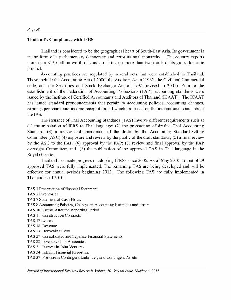
Page 58
Journal of International Business Research, Volume 10, Special Issue, Number 3, 2011
Thailand’s Compliance with IFRS Thailand is considered to be the geographical heart of South-East Asia. Its government is in the form of a parliamentary democracy and constitutional monarchy. The country exports more than $150 billion worth of goods, making up more than two-thirds of its gross domestic product.
Accounting practices are regulated by several acts that were established in Thailand. These include the Accounting Act of 2000, the Auditors Act of 1962, the Civil and Commercial code, and the Securities and Stock Exchange Act of 1992 (revised in 2001). Prior to the establishment of the Federation of Accounting Professions (FAP), accounting standards were issued by the Institute of Certified Accountants and Auditors of Thailand (ICAAT). The ICAAT has issued standard pronouncements that pertain to accounting policies, accounting changes, earnings per share, and income recognition, all which are based on the international standards of the IAS.
The issuance of Thai Accounting Standards (TAS) involve different requirements such as (1) the translation of IFRS to Thai language; (2) the preparation of drafted Thai Accounting Standard; (3) a review and amendment of the drafts by the Accounting Standard-Setting Committee (ASC) (4) exposure and review by the public of the draft standards; (5) a final review by the ASC to the FAP; (6) approval by the FAP; (7) review and final approval by the FAP oversight Committee; and (8) the publication of the approved TAS in Thai language in the Royal Gazette.
Thailand has made progress in adopting IFRSs since 2006. As of May 2010, 16 out of 29 approved TAS were fully implemented. The remaining TAS are being developed and will be effective for annual periods beginning 2013. The following TAS are fully implemented in Thailand as of 2010:
TAS 1 Presentation of financial Statement TAS 2 Inventories TAS 7 Statement of Cash Flows TAS 8 Accounting Policies, Changes in Accounting Estimates and Errors TAS 10 Events After the Reporting Period TAS 11 Construction Contracts TAS 17 Leases TAS 18 Revenue TAS 23 Borrowing Costs TAS 27 Consolidated and Separate Financial Statements TAS 28 Investments in Associates TAS 31 Interest in Joint Ventures TAS 34 Interim Financial Reporting TAS 37 Provisions Contingent Liabilities, and Contingent Assets

Page 59
Journal of International Business Research, Volume 10, Special Issue, Number 3, 2011
TAS 38 Intangible Assets TFRS 3 Business Combinations Full convergence and implementation is expected by January 1, 2013. Thailand’s participation in the convergence of Thai GAAP and IFRS would improve Thailand’s presence in capital markets and continuity with export markets. Vietnam’s Compliance with IFRS
Vietnam is officially known as the Socialist Republic of Vietnam. In 2000, it started developing “diplomatic relations” with most nations having the highest economic growth for the past decade. As of December 2007, Vietnam had developed diplomatic relations with 172 countries and holds membership of 63 international organizations and 650 non-government organizations (Wikipedia, 2010). Listed and unlisted companies in Vietnam are required to use Vietnamese Accounting Standards (VASs) developed by the Ministry of Finance (MoF). Generally, the VASs are based on International Accounting Standards (IASs) that were issued by International Accounting Standards Board (IASB) up to 2003, though some modifications were made to reflect local accounting regulations and environment. The VASs require that accounting records include: (1) the use of Vietnamese language; (2) the use of Vietnamese dong as the accounting currency; (3) compliance with the Vietnam chart of accounts; and (4) present numerous reports as specified by VAS regulations on a monthly basis signed by the General Director and affixed with the company’s seal (Roque, 2009). As of August 2006, none of the IASB amendments to IFRSs or new standards issued after 2003 have been adopted in Vietnam. The MoF announced that Vietnam would continue to formulate 10 new accounting standards in 2008 and will also be developing specific guidelines for small and medium enterprises.
Vietnam is far from complying with IFRS. Up to now, Vietnam continues to use its own standards. Vietnam should realize that full convergence to IFRS will further strengthen its relationship with international companies and will enhance its good and growing economic status.
REFERENCES Accounting (2010, July). Retrieved December 2, 2010, from KPMG: http://www.kpmg.com/CN/
en/IssuesAndInsights/ArticlesPublications/Documents/conversion-to-new-PRC-GAAP-201007.pdf Accountants Today (2008). Full Convergence with IFRS in 2012. Retrieved September 10, 2010 from
http://www.mia.org.my/at/at/200810/06.pdf Accounting & Auditing in Japan. Japanese Institute of Certified Public Accountants (JICPA). (2010)
http://www.hp.jicpa.or.jp/english/accounting/history/development.html Accounting Standards Council (2007). Process of Prescribing Accounting Standards. Retrieved September 23,
2010, from http://www.asc.gov.sg/account.htm
Page 60
Journal of International Business Research, Volume 10, Special Issue, Number 3, 2011
Affairs, B. O. (2010, August 5). US Department of State. Retrieved December 02, 2010, from http://www.state.gov/r/pa/ei/bgn/18902.htm
AICPA IFRS Resources. IFRS for SMEs — U.S. GAAP Comparison Wiki. Retrieved December 20, 2010 from http://wiki.ifrs.com.
Anonymous (2010). Philippines adopt IFRS for SMEs. The Accountant. TA6077 April 2010. International Accounting Bulletin. Retrieved December 20, 2010, from http://www.vrl-financial-news.com/accounting/the-accountant/issues/ta-2010/ta-6077/philippines-adopt-ifrs-for-sme.aspx.
Anonymous (2010). eStandardsForum. Retrieved on September 18, 2010, from http://www.estandardsforum.org/about_research_and_methodology
Anonymous (May 28, 2010). Background Note: South Korea. U.S. Department of State. Retrieved on September 30, 2010, from http://www.state.gov/r/pa/ei/bgn/2800.htm#
Asian Development Bank (1997). Accounting and Auditing in Vietnam. Retrieved from http://www.adb.org/Documents/Books/Financial_Mgt/Vietnam/chap_04.pdf
“Background Note: Malaysia” (2010). Retrieved September 6, 2010 from http://www.state.gov/r/pa/ei/bgn/2777.htm
Baker, N. (2009). Japan Publishes Draft IFRS Roadmap. ComplianceWeek. Retrieved from http://www.complianceweek.com/blog/glimpses/2009/02/24/japan-publishes-draft-ifrs-route-map/
Bangkok Companies Ultimate Contact Database (2002): retrieved 10 29, 2010http://www.bangkokcompanies.com/categories/thai_companies_p165a.htm,
Bobik, M. A. (2010). China's Tourism Industry: A Future Outlook. Grin Verlag Central Intelligence Agency. (2010, November 24). Retrieved December 1, 2010, from
https://www.cia.gov/library/publications/the-world-factbook/geos/ch.html Central Intelligence Agency. (n.d.). The World Fact Book. Retrieved 10 29, 2010, from Central Intelligence Agency:
https://www.cia.gov/library/publications/the-world-factbook/geos/th.html Choi, F.D.S., & Meek, G.K., International Accounting (6th ed.). New Jersey: Pearson Education Inc., 2008 Chong, C. (2009). Compliance of Manufacturing Companies in Manila to Changes in the International Financial
Reporting System (IFRS). Ateneo Press p.11-12 The Constitution of Japan. (2010) House of Counselors. Retrieved from http://www.sangiin.go.jp/eng/law/index.htm Convergence. (2006) IASB and Accounting Standards Board of Japan http://www.ifrs.org/
News/Press+Releases/IASB+and+Accounting+Standards+Board+of+Japan.htm David. (2010, October 6). The US stands by itself on IFRS compliance. Retrieved December 01, 2010, from
http://www.bvwirenews.com/2010/10/06/the-us-stands-by-itself-on-ifrs-compliance/ Deloitte. (2005, April 5). Retrieved December 2, 2010, from IASPLUS: http://www.iasplus.com/dttpubs/
2005ifrsprc.pdf Deloitte. (2010, 01). TFRS Insights-2009 Round Up Issue. Bangkok, Thailand. Economy Watch (n.d.). Retrieved November 30, 2010 from http://www.economywatch.com/world_economy/
indonesia/ Economy Watch (n.d.). Retrieved September 6, 2010 from http://www.economywatch.com/world_economy/
malaysia/ Epstein, Bragg, & Nach (2010). Wiley GAAP: 2011 Interpretation and Application of Generally Accepted
Accounting Principles. Hoboken, NJ: John Wiley & Sons, Inc. Ernst & Young. (2009, January). "US GAAP vs. IFRS." Ernst & Young Global Limited. Retrieved on Sept 30, 2010
http://www.ey.com/Global/assets.nsf/International/IFRS_v_GAAP_basics_Jan09/$file/IFRS_v_GAAP basics_Jan09.pdf
Ernst & Young. (2009). Thailand on the road to IFRS conversion eStandards Forum Financial Standards Foundation. (n.d.). Retrieved December 1, 2010, from Accounting: China: http://www.estandardsforum.org/china/standards/international-financial-reporting-standards

Page 61
Journal of International Business Research, Volume 10, Special Issue, Number 3, 2011
EStandardsforum (2010, August). Philippines: International financial reporting standards. Retrieved Sept. 30, 2010 from http://www.estandardsforum.org/philippines/standards/international-financial-reporting-standards
EStandardsForum (2010). Singapore: International Financial Reporting Standards. February 2010. Retrieved September 23, 2010, from http://www.estandardsforum.org/singapore/standards/international-financial-reporting-standards
EStandardForum Financial Standards Foundation (2009): Retrieved 10 29, http://www.estandardsforum.org/thailand/standards/international-financial-reporting-standards
EStandardsForum (2010). Vietnam: International Financial Reporting Standards. October 2008. Retrieved from http://www.estandardsforum.org/vietnam/standards/international-financial-reporting-standards
FASB Accounting Standards Codification. Retrieved December 20, 2010, from http://asc.fasb.org. Gleeck, L. Jr. (1984) General History of the Philippines: The American Half-Century. Quezon City, R.P.: Garcia.
1984 History of India: From the earliest to the present day. Trotter, Lionel J. January 1872.
http://books.google.com/books?id=Fl8OAAAAQAAJ&printsec=frontcover&dq=history+of+india&hl=en&ei=pW34TKPsMYq2sAPx6aSYAw&sa=X&oi=book_result&ct=result&resnum=2&ved=0CDgQ6AEwAQ#v=onepage&q&f=false. December 2, 2010.
http://www.state.gov/r/pa/ei/bgn/3454.htm http://www.nationsencyclopedia.com/Asia-and-Oceania/India-LOCATION-SIZE-AND-EXTENT.html
http://www.indhistory.com/ Ibarra, V.C. Acc10 Workbook; Theory, short & long problems. Ateneo Press, 2009. P10 IFRS Implementation:
Prepared or Scared? (2010). Retrieved November 30, 2010 from http://docs.google.com/ viewer?a=v&q=cache:YgL5W09jgNkJ
IFRS Standards and Interpretations. Retrieved December 20, 2010, from http://www.ifrs.org/IFRSs/IFRS.htm. Ikatan Akuntan Indonesia (2009). Retrieved November 30, 2010 from http://www.iaiglobal.or.id/
internasional.php?id=14 Indonesia: International Financial Accounting Standards (2009). Retrieved November 30, 2010 from
http://www.estandardsforum.org/indonesia/standards/international-financial-reporting-standards Inews. (2010).Trading with the Philippines: Highlights & restrictions. Retrieved October 01, 2010 from
http://www.iadvisory.com.sg/upload/ups_08oct08.html Jarnagin (2008), 2009 U.S. Master GAAP Guide. Chicago, IL: CCH Group. Janus Corporate Solutions (n.d.). Introduction to Singapore Standards. Retrieved September 23, 2010, from
http://www.guidemesingapore.com/tax/c850-singapore-accounting-standards.htm Japan: History, Geography, Government, & Culture — Infoplease.com http://www.infoplease.com/ipa/
A0107666.html “Malaysia: International Financial Reporting Standards” (2010). Retrieved September 10, 2010 from
http://www.estandardsforum.org/malaysia/standards/international-financial-reporting-standards MASB (2010). Retrieved September 10, 2010 from http://www.masb.org.my/index.php?option=com_
content&view=article&id=3&Itemid=7 Nakamura, Y. (2007). J-GAAP Institutional Background. Accounting Dairy in Japan. Retrieved from
http://accountingdiaryinjapan.blogspot.com/2007/07/j-gaap-institutional-background.html Narongde, P. K. (2010, 10 29). Accounting Professions in Thailand.\ News Release (2007).FASB Retrieved from http://www.fasb.org/news/nr060607.shtml Phuvanatnaranubala, T. (2005, 11 21). PRactical Implementation Issues of International Financial Reporting
\Standards (IFRS). Thailand Price, D. (2010). Hello Work! J@pan Inc. Retrieved from http://www.japaninc.com/print/4368 Price Water Coopers. (2005, 05 26). Adoption in Thailand. Retrieved 10 29, 2010, from pwc:
http://www.pwc.com/th/en/ifrs/pop-up/adoption-popup.jhtml

Page 62
Journal of International Business Research, Volume 10, Special Issue, Number 3, 2011
Price Water Coopers. (2010). IFRS adoption by country. New York City, New York, U.S. Price Water Coopers. (2008). Similarities and Differences: A Comparison of IFRS and Thai GAAP, Vietnamese
GAAP, Cambodia GAAP, and Laos GAAP. PricewaterhouseCoopers LLP (2010). IFRS Adoption by Country. IFRS Reporting. Retrieved December 20, 2010,
from http://www.pwc.com/us/en/issues/ifrs-reporting/assets/ifrs_country_adoption.pdf. Renders A., Gaeremynck A. (2007). The Impact of Legal and Boluntary Investor Protection on the Early Apotion of
International Financial Reporting Standards (IFRS). SpringerLink. Retrieved on September 30, 2010, from http://www.springerlink.com/content/m3765gpt727401p0/abstract/
Republic of Indonesia: Report on the Observance of Standard and Code of Accounting and Auditing (2005). Retrieved November 30, 2010 from http://www.bapepam.go.id/bapepamlk/others/rosc_aa_idn.pdf
Roque, J. (2009). Complying with Vietnam Accounting Standards. Retrieved from http://www.vietnam-briefing.com/news/checking-accounting-compliance.html/
Stickney, Weil, Schipper, & Francis (2007). Financial Accounting: An Introduction to Concepts, Methods, and Uses (Thirteenth Edition). Mason, OH: South-Western Cengage Learning.
Taliaferro, J. (2001). The Emperor of Japan. Heraldica. Retrieved from http://www.heraldica.org/ topics/royalty/japan.htm
Tan, C. (2010) S’pore aims for full IFRS alignment by 2012. Retrieved September 23, 2010,from http://www.timesbusinessdirectory.com/Singlenews.aspx?DirID=86&rec_code=390215
Tohmatsu, D. T. (2002). GAAP Differences in your Pocket: IAS and GAAP in the People's Republic of China. Retrieved from http://www.scribd.com/doc/2606906/ias-gaap-in-china
Tourism Authority of Thailand. (2010). About Thailand. Retrieved 10 09, 2010, from Amazing Thailand: http://www.tourismthailand.org/about-thailand/geography/
Travel Documents Systems, Inc. (n.d.). Retrieved 10 28, 2010, from Travel Documents Systems TDS: http://www.traveldocs.com/th/economy.htm
Tsutsui, W. (2008). The Bubble Economy and the Lost Decade. Japan Society. Retrieved from http://aboutjapan.japansociety.org/content.cfm/the_bubble_economy_and_the_lost_decade_2
Wikipedia (2010). Philippines: Newly industrialize country. Retrieved October 07, 2010 from http://en.wikipedia.org/wiki/Newly_industrialized_country#cite_note-Principles-4
Wikipedia (2010). Singapore. 1 October 2010. Retrieved September 23, 2010, from http://en.wikipedia.org/wiki/Singapore
Wikipedia (2010). Vietnam. 29 November 2010. Retrieved from http://en.wikipedia.org/wiki/Vietnam World Factbook 2009. Washington, DC: Central Intelligence Agency, 2009. https://www.cia.gov/
library/publications/the-world-factbook/index.html
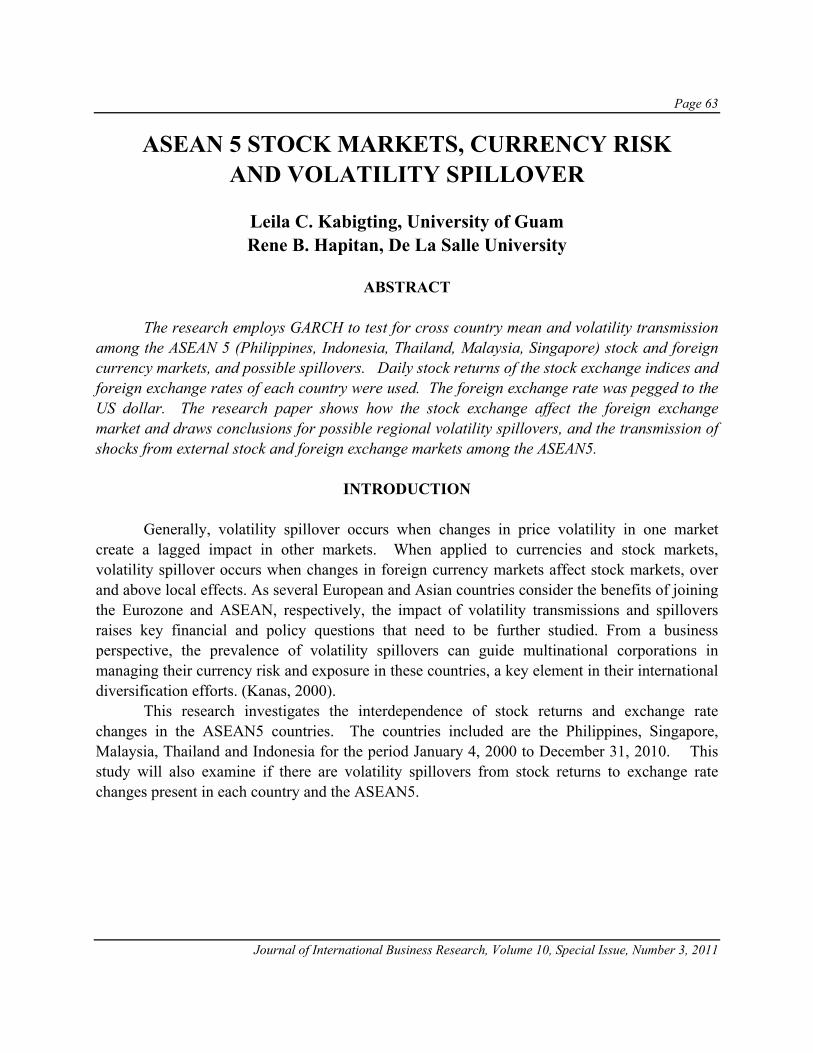
Page 63
Journal of International Business Research, Volume 10, Special Issue, Number 3, 2011
ASEAN 5 STOCK MARKETS, CURRENCY RISK AND VOLATILITY SPILLOVER
Leila C. Kabigting, University of Guam Rene B. Hapitan, De La Salle University
ABSTRACT
The research employs GARCH to test for cross country mean and volatility transmission
among the ASEAN 5 (Philippines, Indonesia, Thailand, Malaysia, Singapore) stock and foreign currency markets, and possible spillovers. Daily stock returns of the stock exchange indices and foreign exchange rates of each country were used. The foreign exchange rate was pegged to the US dollar. The research paper shows how the stock exchange affect the foreign exchange market and draws conclusions for possible regional volatility spillovers, and the transmission of shocks from external stock and foreign exchange markets among the ASEAN5.
INTRODUCTION
Generally, volatility spillover occurs when changes in price volatility in one market create a lagged impact in other markets. When applied to currencies and stock markets, volatility spillover occurs when changes in foreign currency markets affect stock markets, over and above local effects. As several European and Asian countries consider the benefits of joining the Eurozone and ASEAN, respectively, the impact of volatility transmissions and spillovers raises key financial and policy questions that need to be further studied. From a business perspective, the prevalence of volatility spillovers can guide multinational corporations in managing their currency risk and exposure in these countries, a key element in their international diversification efforts. (Kanas, 2000).
This research investigates the interdependence of stock returns and exchange rate changes in the ASEAN5 countries. The countries included are the Philippines, Singapore, Malaysia, Thailand and Indonesia for the period January 4, 2000 to December 31, 2010. This study will also examine if there are volatility spillovers from stock returns to exchange rate changes present in each country and the ASEAN5.
Page 64
Journal of International Business Research, Volume 10, Special Issue, Number 3, 2011
THEORETICAL AND CONCEPTUAL FRAMEWORK The Nature of Volatility Transmission and Volatility Spillover
Two approaches provide the possible link between exchange rates to the other economic and financial sectors. The first, so-called “flow model” looks at the impact of exchange rates on the balance of trade, such as those studied by Mundell in 1963 and by Dornbusch and Fisher in 1980. The flow model posits that changes in exchange rates affect international competitiveness and trade balances, thereby influencing real income and output. Stock prices, generally interpreted as the present values of future cash flows of firms, react to exchange rate changes and form the link among future income, interest rate innovations, and current investment and consumption decisions. (Yang and Doong, 2004) The other model, “stock-oriented” models of exchange rates such as those studied by Branson (1983) and Frankel (1983) models view exchange rates as equating the supply and demand for assets such as stocks and bonds. This approach gives the capital account an important role in determining exchange rate dynamics. Since the values of financial assets are determined by the present values of their future cash flows, expectations of relative currency values play a considerable role in their price movements, especially for internationally held financial assets. Therefore, stock price innovations may affect, or be affected by, exchange rate dynamics. (Ibid, 1984) An illustration of the second approach can be seen in Figure 1, where transmission and spillover is seen as an input-process-output model: Because there has been no dominant approach to explain the impact of volatility spillover, numerous studies have populated the literature in recent years. The residual effect of the Global Financial Crisis still being felt in many countries as well as those “integrated” economies such as the Eurozone and ASEAN provide the motivation for sustained interest in this field of study.
LITERATURE REVIEW
Kanas (1998 and 2000) was one of the first to have examined volatility spillovers in the foreign exchange and stock markets. Using EGARCH, he studied the interdependence of stock returns and exchange rate changes among six industrialized countries, namely the United States (US), the United Kingdom (UK), Japan, Germany, France and Canada. The study concluded that there is evidence of volatility spillovers from stock returns to exchange rates changes for all countries except Germany. However, volatility spillovers from exchange rate changes to stock returns are insignificant for all countries.

Page 65
Journal of International Business Research, Volume 10, Special Issue, Number 3, 2011
Figure 1
Source: Awayan, Guerra, Quipones, Tang Woo. (2010). A Study on the Volatility Transmission in the Exchange Rates of the Currencies of the Philippines, South Korea, and Indonesia and the
Impacts(sic) of the Global and Asian Financial Crises for the Period 1990-2009.
Mishra and Rahman (2010) examined the dynamics of stock market returns volatility of India and Japan using the Threshold Generalized Autoregressive Conditional Heteroskedasticity (TGARCH-M) model. They concluded that return volatility persists in both countries. Savva, Osborn, Gill (2009) used the asymmetric Dynamic Conditional Correlations(DCC) version of the VAR-multivariate Exponential Generalized Autoregressive Conditional Heteroskedasticity (EGARCH) model for daily stock market returns across four major world markets, namely New York, London, Frankfurt and Paris. The results showed that the correlation in the post-euro period was highest between Frankfurt and Paris. Also, the presence of spillover effects from foreign markets for both returns and volatilities exists. The results are consistent with Kanas (1998) where he used the EGARCH model to capture potential asymmetric effects of volatility across the three largest European stock markets, namely London, Frankfurt and Paris. The results showed that there were reciprocal spillovers between London and Paris, and between Paris and Frankfurt, and unidirectional spillovers from London to Frankfurt. Yang and Doong (2004) explored the nature of the mean and volatility transmission mechanism between stock and foreign exchange markets for the G-7 countries. The results point to significant volatility spillovers and an asymmetric effect from the stock market to the foreign exchange market for France, Italy, Japan and the US, suggesting integration between stock and foreign exchange markets in these countries. (O’ Donnell and Morales, n.d.)

Page 66
Journal of International Business Research, Volume 10, Special Issue, Number 3, 2011
Three other studies examined if there are price and volatility spillovers from the US market to other countries. In the case of Hong Kong, Singapore, Taiwan and Malaysia except Korea, there was a decrease in price and volatility spillovers from the US market since the 1997 Asian financial crisis. The study used the EGARCH model for the prior- and post-crisis periods. Data is the daily stock prices from January 3, 1995 to April 24 2001. (Nam, Yuhn, and Kim, 2008). In the case of Europe and the US, Anaraki, (n.d.) investigated the link by using Granger causality. The causality runs from the US to European stock market and that the US fundamentals including the Federal Fund Rate (FFR), the Euro-dollar exchange rate, and the US stock market indices affect European stock market volatility. Using a multivariate generalized autoregressive conditional heteroskedasticity (GARCH-M) model, Chancharoenchai and Dibooglu (2006) examined volatility spillovers in six Southeast Asian stock markets pre and after the 1997 Asian crisis and its interactions with the U.S. market (using the New York Stock Exchange as the global market), Japan (using the Tokyo Stock Exchange as a regional market). The study concluded that there were some interdependence in volatility between emerging markets and developed markets before and after crisis. The study showed evidence of the Asian contagion which started in Thailand and affected other financial markets. Most of the literature on the international interactions of stock returns, foreign exchange rate changes and volatility spillovers employ Generalized Autoregressive Conditional Heteroskedasticity (GARCH) models (Bollerslev, 1986). These models determine if there is volatility clustering, fat tails, volatility spillover. Volatility clustering in asset returns means that “large price changes follow large price changes of either sign and small price changes follow small prices changes of either sign.” (Mandelbrot , 1963). The GARCH (1,1) is often used since the model is parsimonious. Another GARCH model was developed by Nelson (1991), the Exponential GARCH to study the asymmetrical effects of shocks on stock return volatility, known as leverage effect. The results showed that negative shocks have larger effects on volatility than positive shocks. (Kanas 1998).
METHODOLOGY
We used daily closing stock prices denominated in local currency for the Philippines Stock Exchange Index (denoted in the runs as PSEi) in the case of the Philippines, the FTSE Straits Times Index (denoted as FSSTI Index) for Singapore, the FTSE Bursa Malaysia KLCI Index (denoted as FBMKLCI) for Malaysia, the Stock Exchange of Thailand (denoted as SET) for Thailand, and the Jakarta Composite Index (denoted as JCI Index) for Indonesia for the period from 4 January 2000 to 31 December 2010. The stock indices are not adjusted for dividends since they will not affect the results (Kanas, 2000). For exchange rate, the currencies used were: the Philippine Peso, Indonesian Rupiah, Singapore Dollar, Thai Baht and Malaysian Ringgit. The exchange rate series for each country and indices were all derived from Bloomberg.

Page 67
Journal of International Business Research, Volume 10, Special Issue, Number 3, 2011
Following Kanas (2000), we compute for the stock returns (denoted as ret in the results) and exchange rate changes (denoted by St and E t, respectively) are calculated as the difference between the natural logarithms of the closing values for two consecutive trading days, i.e. St = ln(P
S t) - ln(PS
t-1), and Et = ln(PEt) – ln (PE
t-1), where PSt and PE
t are the stock price and the exchange rate at period t, respectively. GARCH (1,1) specification was used since it is a parsimonious representation of conditional variance of time series data (Bollerslev, 1987), in this case, the stock returns and foreign exchange changes.
RESEARCH FINDINGS: MODEL RESULTS
Descriptive statistics for stock returns of the indices are reported in Table 1. The sample means of returns are positive and statistically different from zero. The variances range from 0.009 (Malaysia) to 0.1525 (Indonesia). The measures for skewness indicate that all countries except the Philippines (PSEi) are negatively skewed and excess kurtosis indicate that the distributions of returns for all markets are leptokurtic.
Table 1: Summary Statistics, Stock Returns using the observations 2000/01/04 - 2010/12/30
(missing values were skipped) Variable Mean Median Minimum Maximum retpsei 0.000246919 0.000107464 -0.130887 0.161776 retjciindex 0.000624071 0.00127921 -0.109540 0.0762312 retset 0.000270504 0.000404790 -0.160633 0.105770 retfbmklci 0.000221836 0.000462797 -0.0997851 0.0450273 retfSSTI Index 8.12490e-005 0.000449251 -0.0869598 0.0753053 Variable Std. Dev. C.V. Skewness Ex. kurtosis retpsei 0.0143023 57.9230 0.500516 15.6014 retjciindex 0.0152522 24.4399 -0.627927 5.67023 retset 0.0151458 55.9912 -0.756638 8.99236 retfbmklci 0.00940011 42.3741 -0.863193 9.14827 retfSSTI Index 0.0132466 163.037 -0.241634 4.36202
Descriptive statistics for foreign exchange rate changes are reported in Table 2. The
sample means of returns are positive except for Malaysia and Singapore and statistically different from zero. The variances range from 0.0000208 (Thailand) to 0.007 (Indonesia) The measures for skewness indicate that all countries except Thailand are negatively skewed and excess kurtosis indicate that the distributions of the foreign exchange rate changes for all markets are leptokurtic.
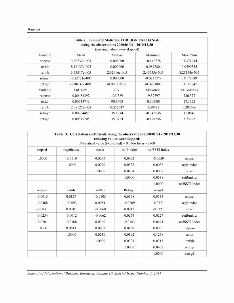
Page 68
Journal of International Business Research, Volume 10, Special Issue, Number 3, 2011
Table 2: Summary Statistics, FOREIGN EXCHANGE, using the observations 2000/01/04 - 2010/12/30
(missing values were skipped) Variable Mean Median Minimum Maximum retpeso 3.60732e-005 0.000000 -0.142778 0.0371944 retidr 8.16137e-005 0.000000 -0.0897804 0.0590335 retthb 3.63517e-005 2.62916e-005 2.46655e-005 8.21164e-005 retmyr -7.52771e-005 0.000000 -0.0231778 0.0175549 retsgd -8.88746e-005 -0.000115380 -0.0203807 0.0157647
Variable Std. Dev. C.V. Skewness Ex. kurtosis retpeso 0.00488392 135.389 -9.52797 280.322 retidr 0.00735742 90.1493 -0.395801 17.1222 retthb 2.08127e-005 0.572537 1.50691 0.293686 retmyr 0.00264459 35.1314 -0.345536 11.0646 retsgd 0.00311705 35.0724 -0.179246 3.74293
Table 3: Correlation coefficients, using the observations 2000/01/04 - 2010/12/30 (missing values were skipped)
5% critical value (two-tailed) = 0.0366 for n = 2868
retpsei retjciindex retset retfbmklci retfSSTI Index
1.0000 -0.0119 0.0099 0.0092 -0.0059 retpsei
1.0000 0.0270 0.0323 0.0036 retjciindex
1.0000 0.0184 0.0002 retset
1.0000 0.0538 retfbmklci
1.0000 retfSSTI Index
retpeso retidr retthb Retmyr retsgd
-0.0015 0.0127 -0.0105 0.0278 0.0134 retpsei
-0.0468 -0.0093 0.0054 -0.0209 -0.0371 retjciindex
-0.0031 0.0010 -0.0068 0.0012 -0.0121 retset
-0.0254 -0.0012 -0.0062 0.0274 0.0227 retfbmklci
-0.0261 -0.0168 0.0360 -0.0163 0.0441 retfSSTI Index
1.0000 0.0613 0.0002 0.0169 0.0055 retpeso
1.0000 0.0230 0.0192 0.1268 retidr
1.0000 0.0304 0.0315 retthb
1.0000 0.0452 retmyr
1.0000 retsgd

Page 69
Journal of International Business Research, Volume 10, Special Issue, Number 3, 2011
Table 3 shows the correlation coefficient for each variable. The PSEi stock return is negatively correlated to the Indonesian and Singaporean stock returns, while positively correlated to Malaysian and Thai stock returns. The Malaysian, Indonesian, Thai, and Singaporean stock returns are positively correlated to each other. The foreign exchange rate change, retpeso (Philippines) is negatively correlated to all countries’ stock returns including the retpsei (Philippines). The Indonesian rupiah and Thai baht foreign exchange rate changes are also negatively correlated with their respective stock returns on the indices. Singapore dollar and Malaysia ringgit foreign exchange rate changes are positively correlated with their respective stock returns on the indices. An increase in the foreign exchange in one country is viewed as favorable in the other. This is typical of these two countries as both are active trading and financial partners.
TABLE 4: Model 1 ARCH, using observations 2000/01/05-2010/05/11 (T = 2700)
Dependent variable: retpsei Standard errors based on Hessian
Coefficient Std. Error z p-value const 0.000409585 0.00023327 1.7558 0.07912 * retpeso -0.42622 0.0382203 -11.1517 <0.00001 *** alpha(0) 1.46418e-05 2.48929e-06 5.8819 <0.00001 *** alpha(1) 0.199983 0.0211614 9.4504 <0.00001 *** beta(1) 0.746274 0.023964 31.1415 <0.00001 *** Mean dependent var 0.000235 S.D. dependent var 0.014317 Log-likelihood 7870.915 Akaike criterion -15729.83 Schwarz criterion -15694.42 Hannan-Quinn -15717.03 Unconditional error variance = 0.00027244
Table 5: Model 2: GARCH, using observations 2000/01/04-2010/03/26 (T = 2669)
Dependent variable: retjciindex Standard errors based on Hessian
Coefficient Std. Error z p-value
const 0.00132724 0.000251939 5.2681 <0.00001 ***
retidr -0.049531 0.0331003 -1.4964 0.13455
alpha(0) 1.4793e-05 2.71361e-06 5.4514 <0.00001 ***
alpha(1) 0.141121 0.017445 8.0895 <0.00001 ***
beta(1) 0.795718 0.0239791 33.1839 <0.00001 ***
Mean dependent var 0.000624 S.D. dependent var 0.015252
Log-likelihood 7634.732 Akaike criterion -15257.46
Schwarz criterion -15222.13 Hannan-Quinn -15244.68
Unconditional error variance = 0.000234213

Page 70
Journal of International Business Research, Volume 10, Special Issue, Number 3, 2011
Table 4 shows the results of GARCH (1,1) for retpsei and retpeso. The p-value is significant. Also, volatility spillover exists between the Philippine stock market to the Philippine foreign exchange rate based on the alpha and beta results.
Table 5 shows the results of GARCH (1,1) for retjcindex and retidr. The p-value is not significant. Also, volatility spillover exists between the Indonesian stock market to the Indonesian foreign exchange rate based on the alpha and beta results.
Table 6: Model 3: GARCH, using observations 2000/01/04-2010/04/29 (T = 2693) Dependent variable: retset
Standard errors based on Hessian
Coefficient Std. Error z p-value
const 0.000761275 0.000506557 1.5028 0.13288
retthb 4.06065 11.9368 0.3402 0.73372
alpha(0) 2.03909e-05 3.41554e-06 5.9700 <0.00001 ***
alpha(1) 0.120092 0.0165926 7.2377 <0.00001 ***
beta(1) 0.786669 0.0274207 28.6888 <0.00001 ***
Mean dependent var 0.000271 S.D. dependent var 0.015146
Log-likelihood 7685.133 Akaike criterion -15358.27
Schwarz criterion -15322.87 Hannan-Quinn -15345.47
Unconditional error variance = 0.000218695
Table 6 shows the results of GARCH (1,1) for retset and retthb. The p-value is not
significant. Also, volatility spillover exists between the Thai stock market to the Thai foreign exchange rate based on the alpha and beta results.
Table 7: Model 4: GARCH, using observations 2000/01/05-2010/05/24 (T = 2709) Dependent variable: retfbmklci
Standard errors based on Hessian
Coefficient Std. Error z p-value
const 0.000577577 0.000134222 4.3032 0.00002 ***
retmyr 0.0824977 0.0474972 1.7369 0.08241 *
alpha(0) 1.07521e-06 3.17802e-07 3.3833 0.00072 ***
alpha(1) 0.123606 0.0158681 7.7896 <0.00001 ***
beta(1) 0.874124 0.0153776 56.8439 <0.00001 ***
Mean dependent var 0.000222 S.D. dependent var 0.009400
Log-likelihood 9185.873 Akaike criterion -18359.75
Schwarz criterion -18324.32 Hannan-Quinn -18346.94
Unconditional error variance = 0.000473662

Page 71
Journal of International Business Research, Volume 10, Special Issue, Number 3, 2011
Table 7 shows the results of GARCH (1,1) for retfblmklc and retmyr. The p-value is significant. Also, volatility spillover exists between the Malaysian stock market and the Malaysian foreign exchange rate based on the alpha and beta results.
Table 8: Model 5: GARCH, using observations 2000/01/05-2010/08/04 (T = 2761) Dependent variable: retFSSTI Index
Standard errors based on Hessian
Coefficient Std. Error z p-value
const 0.000547155 0.000181741 3.0106 0.00261 ***
retsgd 0.0263514 0.0624312 0.4221 0.67296
alpha(0) 1.4354e-06 4.16955e-07 3.4426 0.00058 ***
alpha(1) 0.0998542 0.0107854 9.2582 <0.00001 ***
beta(1) 0.895657 0.0102046 87.7703 <0.00001 ***
Mean dependent var 0.000081 S.D. dependent var 0.013247
Log-likelihood 8451.841 Akaike criterion -16891.68
Schwarz criterion -16856.14 Hannan-Quinn -16878.84
Unconditional error variance = 0.000319773
Table 8 shows the results of GARCH (1,1) for retFSSTI Index and retsgd. The p-value is
not significant. Also, volatility spillover exists between the Singaporean stock market and the Singaporean foreign exchange rate based on the alpha and beta results.
Table 9: Model 6: GARCH, using observations 2000/01/05-2010/05/11 (T = 2700)
Dependent variable: retpeso Standard errors based on Hessian
Coefficient Std. Error z p-value
const 8.07153e-05 5.00607e-05 1.6123 0.10689
retpsei -0.00129963 0.00390811 -0.3325 0.73948
alpha(0) 3.47397e-07 7.30592e-08 4.7550 <0.00001 ***
alpha(1) 0.222078 0.0180842 12.2802 <0.00001 ***
beta(1) 0.777922 0.0174963 44.4620 <0.00001 ***
Mean dependent var 0.000032 S.D. dependent var 0.004881
Log-likelihood 11572.62 Akaike criterion -23133.24
Schwarz criterion -23097.83 Hannan-Quinn -23120.43
Unconditional error variance = 6.16567e+007

Page 72
Journal of International Business Research, Volume 10, Special Issue, Number 3, 2011
Table 10: Model 7: GARCH, using observations 2000/01/04-2010/03/26 (T = 2669) Dependent variable: retidr
Standard errors based on Hessian Coefficient Std. Error z p-value
const 3.43288e-05 9.40919e-05 0.3648 0.71523
retjciindex -0.00515879 0.00555879 -0.9280 0.35339
alpha(0) 3.44955e-06 4.37192e-07 7.8902 <0.00001 ***
alpha(1) 0.335201 0.0305775 10.9623 <0.00001 ***
beta(1) 0.664799 0.0261348 25.4373 <0.00001 ***
Mean dependent var 0.000089 S.D. dependent var 0.007566
Log-likelihood 9832.963 Akaike criterion -19653.93
Schwarz criterion -19618.59 Hannan-Quinn -19641.14
Unconditional error variance = 960324
Table 11: Model 8: GARCH, using observations 2000/01/05-2010/08/04 (T = 2761) Dependent variable: retsgd
Standard errors based on Hessian Coefficient Std. Error z p-value
const -0.000105167 5.12557e-05 -2.0518 0.04019 **
retfSSTI Index 0.00627846 0.00401432 1.5640 0.11781
alpha(0) 1.06892e-07 3.26818e-08 3.2707 0.00107 ***
alpha(1) 0.0437789 0.0069778 6.2740 <0.00001 ***
beta(1) 0.945068 0.00892546 105.8844 <0.00001 ***
Mean dependent var -0.000073 S.D. dependent var 0.003088
Log-likelihood 12246.09 Akaike criterion -24480.17
Schwarz criterion -24444.63 Hannan-Quinn -24467.34
Unconditional error variance = 9.58388e-006
Tables 9, 10, and 11 show that volatility spillovers from exchange rate changes to stock returns are significant for Singapore, Indonesia and the Philippines. However, software runs for Malaysia and Thailand resulted into error despite several attempts. This implies that the convergence criterion was not present.

Page 73
Journal of International Business Research, Volume 10, Special Issue, Number 3, 2011
Table 12: Model 9: GARCH, using observations 2000/01/05-2010/03/26 (T = 2668) Dependent variable: retPSEi
Standard errors based on Hessian
Coefficient Std. Error z p-value
Const 0.051502 0.0315025 1.6349 0.10208
retfSSTI Index 0.151885 1.3426 0.1131 0.90993
retjciindex -0.759426 1.0524 -0.7216 0.47053
Retset -0.0530194 1.16144 -0.0456 0.96359
retfbmklci -1.07831 1.8491 -0.5832 0.55979
Retpeso -30.5301 2.70618 -11.2816 <0.00001 ***
Retidr 1.94724 2.1933 0.8878 0.37464
Retthb -549.092 735.818 -0.7462 0.45553
Retmyr 9.85199 7.1398 1.3799 0.16763
Retsgd -2.01639 5.45151 -0.3699 0.71147
alpha(0) 0.068975 0.011935 5.7792 <0.00001 ***
alpha(1) 0.202876 0.0214085 9.4764 <0.00001 ***
beta(1) 0.746174 0.0239392 31.1695 <0.00001 ***
Mean dependent var 0.017888 S.D. dependent var 0.999071
Log-likelihood -3541.332 Akaike criterion 7110.664
Schwarz criterion 7193.112 Hannan-Quinn 7140.498
Unconditional error variance = 1.35378
Table 13: Model 10: GARCH, using observations 2000/01/05-2010/03/26 (T = 2668) Dependent variable: retjciindex
Standard errors based on Hessian
Coefficient Std. Error z p-value
const 0.00110156 0.000494091 2.2295 0.02578 **
retfSSTI Index -0.0136058 0.0192688 -0.7061 0.48012
retset 0.0138238 0.0183159 0.7547 0.45040
retfbmklci 0.0432274 0.0286173 1.5105 0.13091
retpeso -0.0389996 0.0556795 -0.7004 0.48366
retidr -0.0404195 0.0337233 -1.1986 0.23070
retthb 4.9839 11.6034 0.4295 0.66754
retmyr -0.158373 0.109879 -1.4413 0.14949
retsgd -0.130468 0.0840113 -1.5530 0.12043
retPSEi -0.0222121 0.018222 -1.2190 0.22285

Page 74
Journal of International Business Research, Volume 10, Special Issue, Number 3, 2011
Table 13: Model 10: GARCH, using observations 2000/01/05-2010/03/26 (T = 2668) Dependent variable: retjciindex
Standard errors based on Hessian
Coefficient Std. Error z p-value
alpha(0) 1.50416e-05 2.75839e-06 5.4530 <0.00001 ***
alpha(1) 0.141404 0.0176693 8.0028 <0.00001 ***
beta(1) 0.793987 0.0243974 32.5440 <0.00001 ***
Mean dependent var 0.000636 S.D. dependent var 0.015242
Log-likelihood 7638.708 Akaike criterion -15249.42
Schwarz criterion -15166.97 Hannan-Quinn -15219.58
Unconditional error variance = 0.000232811
Table 14: Model 11: GARCH, using observations 2000/01/05-2010/03/26 (T = 2668) Dependent variable: retset
Standard errors based on Hessian
Coefficient Std. Error z p-value
const 0.00112611 0.000507964 2.2169 0.02663 **
retfSSTI Index 0.0126462 0.020667 0.6119 0.54060
retfbmklci 0.0462272 0.029768 1.5529 0.12044
retpeso 0.0686826 0.0636375 1.0793 0.28046
retidr -0.020453 0.0368582 -0.5549 0.57896
retthb -5.33834 11.9532 -0.4466 0.65516
retmyr 0.193123 0.118983 1.6231 0.10456
retsgd 1.95525e-05 0.0877279 0.0002 0.99982
retPSEi -0.00648415 0.0189839 -0.3416 0.73268
retjciindex 0.0229849 0.0197718 1.1625 0.24503
alpha(0) 2.04548e-05 3.49307e-06 5.8558 <0.00001 ***
alpha(1) 0.128036 0.0191421 6.6887 <0.00001 ***
beta(1) 0.780403 0.0291884 26.7367 <0.00001 ***
Mean dependent var 0.000289 S.D. dependent var 0.015139
Log-likelihood 7615.112 Akaike criterion -15202.22
Schwarz criterion -15119.78 Hannan-Quinn -15172.39
Unconditional error variance = 0.0002234

Page 75
Journal of International Business Research, Volume 10, Special Issue, Number 3, 2011
Tables 12, 13, and 14 show that the stock returns for the Philippine, Indonesian and Singaporean markets have persistent volatility and that there are spillovers to the other stock markets and foreign exchange rates. This means that the ASEAN5 stock market and foreign exchange markets are integrated and that any news on these markets will affect the other countries’ markets. The study included a GARCH (1,1) specification for both the stock returns on indices and foreign exchange changes to cover a subperiod starting June 1, 2007. On June 2007, Bear Sterns were forced to sell assets after their hedge funds with large holdings of subprime mortgages suffered large losses(Guillen, n.d). We will use this date as a subperiod to determine if volatility persists during the start of a global financial crisis and if there are evidences of volatility spillovers until the end of December 2010.
Table 15: Model 12: GARCH, using observations 2007/06/01-2010/08/11 (T = 834) Dependent variable: retpsei
Standard errors based on Hessian
Coefficient Std. Error z p-value
Const 0.000981244 0.000447434 2.1931 0.02830 **
Retjci -0.0271703 0.0246361 -1.1029 0.27009
Retset -0.00408886 0.0313633 -0.1304 0.89627
retfbmklci_inde 0.0731688 0.0638906 1.1452 0.25212
Retfssti -0.0104083 0.0293733 -0.3543 0.72308
Retidr 0.0611328 0.0614346 0.9951 0.31969
Retmyr -0.215454 0.111388 -1.9343 0.05308 *
Retsgd 0.0682212 0.123933 0.5505 0.58200
Retpeso 0.158323 0.107717 1.4698 0.14161
Retthb -0.0623793 0.143085 -0.4360 0.66287
alpha(0) 9.10178e-06 3.96753e-06 2.2941 0.02179 **
alpha(1) 0.150747 0.0319415 4.7195 <0.00001 ***
beta(1) 0.819348 0.0388831 21.0721 <0.00001 ***
Mean dependent var 0.000247 S.D. dependent var 0.016347
Log-likelihood 2360.239 Akaike criterion -4692.477
Schwarz criterion -4626.310 Hannan-Quinn -4667.109
Unconditional error variance = 0.000304357

Page 76
Journal of International Business Research, Volume 10, Special Issue, Number 3, 2011
Table 16: Model 13: GARCH, using observations 2007/06/01-2010/08/11 (T = 834) Dependent variable: retjci
Standard errors based on Hessian
Coefficient Std. Error z p-value
Const 0.00119088 0.000506397 2.3517 0.01869 **
Retset 0.0259006 0.0355295 0.7290 0.46601
retfbmklci_inde 0.0556889 0.0560895 0.9929 0.32078
Retfssti 0.00152385 0.0296245 0.0514 0.95898
Retidr 0.00719751 0.0712532 0.1010 0.91954
Retmyr -0.247524 0.122619 -2.0186 0.04352 **
Retsgd 0.243843 0.14483 1.6837 0.09225 *
Retpeso 0.0816309 0.106845 0.7640 0.44486
Retthb -0.0707309 0.17237 -0.4103 0.68155
Retpsei -0.0254544 0.0334898 -0.7601 0.44722
alpha(0) 1.29768e-05 3.87661e-06 3.3475 0.00082 ***
alpha(1) 0.14556 0.0263961 5.5144 <0.00001 ***
beta(1) 0.817742 0.0290423 28.1569 <0.00001 ***
Mean dependent var 0.000554 S.D. dependent var 0.018595
Log-likelihood 2262.394 Akaike criterion -4496.789
Schwarz criterion -4430.622 Hannan-Quinn -4471.420
Unconditional error variance = 0.000353605
Table 17: Model 14: GARCH, using observations 2007/06/01-2010/08/11 (T = 834) Dependent variable: retset
Standard errors based on Hessian
Coefficient Std. Error Z p-value
const 0.00125671 0.000441034 2.8495 0.00438 ***
retfbmklci_inde -0.0220331 0.0482013 -0.4571 0.64760
retfssti -0.00241563 0.028872 -0.0837 0.93332
retidr 0.0289232 0.0725929 0.3984 0.69031
retmyr 0.200491 0.114925 1.7445 0.08106 *
retsgd -0.0535125 0.136243 -0.3928 0.69449
retpeso -0.213458 0.102941 -2.0736 0.03812 **
retthb -0.230843 0.144696 -1.5954 0.11063
retpsei 0.0100106 0.0304021 0.3293 0.74195
retjci 0.018723 0.0282761 0.6621 0.50788
alpha(0) 5.13683e-06 2.02241e-06 2.5400 0.01109 **

Page 77
Journal of International Business Research, Volume 10, Special Issue, Number 3, 2011
Table 17: Model 14: GARCH, using observations 2007/06/01-2010/08/11 (T = 834) Dependent variable: retset
Standard errors based on Hessian
Coefficient Std. Error Z p-value
alpha(1) 0.119977 0.0208121 5.7648 <0.00001 ***
beta(1) 0.863977 0.0205942 41.9524 <0.00001 ***
Mean dependent var 0.000319 S.D. dependent var 0.016576
Log-likelihood 2357.312 Akaike criterion -4686.625
Schwarz criterion -4620.458 Hannan-Quinn -4661.257
Unconditional error variance = 0.000320141
Table 18: Model 15: GARCH, using observations 2007/06/01-2010/08/11 (T = 834) Dependent variable: retfbmklci_inde
Standard errors based on Hessian
Coefficient Std. Error Z p-value
const 0.000758725 0.000252621 3.0034 0.00267 ***
retfssti 0.0113419 0.0168251 0.6741 0.50024
retidr 0.0254291 0.0365779 0.6952 0.48693
retmyr -0.0187246 0.0607504 -0.3082 0.75791
retsgd 0.0460012 0.0720567 0.6384 0.52321
retpeso -0.187645 0.0627862 -2.9886 0.00280 ***
retthb -0.0611178 0.0836623 -0.7305 0.46507
retpsei 0.0289376 0.0199808 1.4483 0.14754
retjci 0.0126959 0.0158835 0.7993 0.42411
retset -0.0129801 0.0181719 -0.7143 0.47504
alpha(0) 1.70056e-06 7.68163e-07 2.2138 0.02684 **
alpha(1) 0.174617 0.028838 6.0551 <0.00001 ***
beta(1) 0.825383 0.0272578 30.2806 <0.00001 ***
Mean dependent var 0.000107 S.D. dependent var 0.010085
Log-likelihood 2785.127 Akaike criterion -5542.253
Schwarz criterion -5476.086 Hannan-Quinn -5516.885
Unconditional error variance = 1.84212e+007

Page 78
Journal of International Business Research, Volume 10, Special Issue, Number 3, 2011
Table 19: Model 16: : GARCH, using observations 2007/06/01-2010/08/11 (T = 834) Dependent variable: retfssti
Standard errors based on Hessian
Coefficient Std. Error Z p-value
const 0.000500276 0.000402032 1.2444 0.21336
retpsei -0.033138 0.0289111 -1.1462 0.25171
retjci 0.0289614 0.0210753 1.3742 0.16938
retidr 0.00101502 0.0738605 0.0137 0.98904
retpeso -0.0630895 0.0864475 -0.7298 0.46551
retthb -0.22987 0.117993 -1.9482 0.05140 *
retmyr 0.176334 0.105469 1.6719 0.09454 *
retsgd 0.0108712 0.131793 0.0825 0.93426
retset 0.00896206 0.0252185 0.3554 0.72231
retfbmklci_inde 0.0866703 0.0445245 1.9466 0.05159 *
alpha(0) 2.35098e-06 1.30289e-06 1.8044 0.07116 *
alpha(1) 0.13431 0.0230304 5.8319 <0.00001 ***
beta(1) 0.863584 0.0209251 41.2703 <0.00001 ***
Mean dependent var -0.000149 S.D. dependent var 0.016893
Log-likelihood 2373.436 Akaike criterion -4718.871
Schwarz criterion -4652.704 Hannan-Quinn -4693.503
Unconditional error variance = 0.00111672
Tables 15, 16, 17, 18, 19 show that the p-value of the retmyr is significant in all stock
returns on indices except for Malaysia. The retmyr has a positive relationship with both the Singaporean and Thai stock returns on indices. The retmyr has a negative relationship with both the Philippine and Indonesian stock returns on indices.
Table 16 shows that the p-value of retsgd is significant and has a positive relationship with retjci. Table 17 and 18 show that the p-value of retpeso is significant and has a negative relationship with retset and retfbmklci_inde, respectively. Table 19 shows that the p-value of retthb is significant and has a negative relationship with retfssti. Tables 15, 16, 17,18, and 19 show that volatility is persistent and that there are spillovers to the other stock markets and foreign exchange rates. The alpha and beta values are higher during this subperiod of the financial crisis which indicates that the market takes time to absorb the impact of information and volatility persists.

Page 79
Journal of International Business Research, Volume 10, Special Issue, Number 3, 2011
Table 20: Model 17: GARCH, using observations 2007/06/01-2010/08/11 (T = 834) Dependent variable: retpeso
Standard errors based on Hessian
Coefficient Std. Error z p-value
Const -4.53241e-05 0.000144234 -0.3142 0.75334
Retidr 0.0108114 0.0201272 0.5372 0.59116
Retmyr 0.0209637 0.0364225 0.5756 0.56491
Retsgd 0.0149479 0.0386298 0.3870 0.69879
retthb -0.111454 0.0469043 -2.3762 0.01749 **
retpsei 0.00495771 0.00973482 0.5093 0.61056
retjci 0.00926667 0.00805189 1.1509 0.24979
retset -0.0135335 0.00936735 -1.4447 0.14853
retfbmklci_inde -0.0322533 0.0151236 -2.1326 0.03295 **
retfssti -0.00772692 0.00863735 -0.8946 0.37100
alpha(0) 6.28294e-07 3.02312e-07 2.0783 0.03768 **
alpha(1) 0.103505 0.0253881 4.0769 0.00005 ***
beta(1) 0.867795 0.0306009 28.3585 <0.00001 ***
Mean dependent var -0.000076 S.D. dependent var 0.004605
Log-likelihood 3342.952 Akaike criterion -6657.903
Schwarz criterion -6591.736 Hannan-Quinn -6632.535
Unconditional error variance = 2.1892e-005
Table 21: Model 18: GARCH, using observations 2007/06/01-2010/08/11 (T = 834) Dependent variable: retidr
Standard errors based on Hessian
Coefficient Std. Error Z p-value
const -5.24677e-05 0.000139118 -0.3771 0.70607
retmyr 0.184379 0.0450983 4.0884 0.00004 ***
retsgd -0.0168322 0.0449055 -0.3748 0.70778
retthb 0.00859123 0.0315043 0.2727 0.78508
retpsei -0.00255088 0.00691328 -0.3690 0.71214
retjci -0.00785515 0.00694385 -1.1312 0.25796
retset 0.00661844 0.00652647 1.0141 0.31054
retfbmklci_inde -0.00176059 0.0120432 -0.1462 0.88377
retfssti 0.0155717 0.00661603 2.3536 0.01859 **
Retpeso 0.0328715 0.0265139 1.2398 0.21506
alpha(0) 5.78678e-07 1.69907e-07 3.4058 0.00066 ***

Page 80
Journal of International Business Research, Volume 10, Special Issue, Number 3, 2011
Table 21: Model 18: GARCH, using observations 2007/06/01-2010/08/11 (T = 834) Dependent variable: retidr
Standard errors based on Hessian
Coefficient Std. Error Z p-value
alpha(1) 0.149061 0.0290481 5.1315 <0.00001 ***
beta(1) 0.846949 0.025351 33.4089 <0.00001 ***
Mean dependent var -0.000013 S.D. dependent var 0.006830
Log-likelihood 3243.926 Akaike criterion -6459.851
Schwarz criterion -6393.684 Hannan-Quinn -6434.483
Unconditional error variance = 0.000145035
Table 22: Model 19: GARCH, using observations 2007/06/01-2010/08/11 (T = 834) Dependent variable: retthb
Standard errors based on Hessian
Coefficient Std. Error z p-value
const -8.62565e-05 6.80432e-05 -1.2677 0.20491
retmyr 0.0016322 0.0185389 0.0880 0.92984
retsgd 0.238865 0.0258216 9.2506 <0.00001 ***
retpsei -0.00757537 0.00522802 -1.4490 0.14734
retjci -0.00165233 0.00440304 -0.3753 0.70746
retset -0.0121791 0.00494023 -2.4653 0.01369 **
retfbmklci_inde -0.00918824 0.00676398 -1.3584 0.17433
retfssti -0.00685871 0.00439909 -1.5591 0.11897
retpeso -0.0548585 0.0172497 -3.1803 0.00147 ***
retidr -0.00316257 0.012035 -0.2628 0.79272
alpha(0) 3.28729e-07 1.08083e-07 3.0415 0.00235 ***
alpha(1) 0.262849 0.0452133 5.8135 <0.00001 ***
beta(1) 0.737151 0.0403357 18.2754 <0.00001 ***
Mean dependent var -0.000124 S.D. dependent var 0.003580
Log-likelihood 3794.682 Akaike criterion -7561.364
Schwarz criterion -7495.197 Hannan-Quinn -7535.996
Unconditional error variance = 1.92831e+006

Page 81
Journal of International Business Research, Volume 10, Special Issue, Number 3, 2011
Table 23: Model 20: GARCH, using observations 2007/06/01-2010/08/11 (T = 834) Dependent variable: retmyr
Standard errors based on Hessian
Coefficient Std. Error z p-value
const -0.000193129 0.000112758 -1.7128 0.08675 *
retsgd 0.0677273 0.0384396 1.7619 0.07808 *
retpsei 0.00548671 0.0067486 0.8130 0.41621
retjci -5.19301e-05 0.00634895 -0.0082 0.99347
retset -0.000655657 0.00756114 -0.0867 0.93090
retfbmklci_inde -0.00225435 0.0109943 -0.2050 0.83753
retfssti -0.00874604 0.00662814 -1.3195 0.18699
retpeso 0.0171017 0.0234216 0.7302 0.46529
retidr 0.0770925 0.0235447 3.2743 0.00106 ***
retthb 0.0108206 0.0254415 0.4253 0.67061
alpha(0) 3.07789e-07 1.4771e-07 2.0837 0.03718 **
alpha(1) 0.124471 0.0322547 3.8590 0.00011 ***
beta(1) 0.868968 0.02823 30.7817 <0.00001 ***
Mean dependent var -0.000097 S.D. dependent var 0.003919
Log-likelihood 3490.296 Akaike criterion -6952.592
Schwarz criterion -6886.425 Hannan-Quinn -6927.224
Unconditional error variance = 4.69133e-005
Table 24: Model 21: GARCH, using observations 2007/06/01-2010/08/11 (T = 834) Dependent variable: retsgd
Standard errors based on Hessian
Coefficient Std. Error z p-value
const -0.000118557 9.95123e-05 -1.1914 0.23351
retpsei -0.000798756 0.00604538 -0.1321 0.89488
retjci 0.00982239 0.00544697 1.8033 0.07134 *
retset 0.00354235 0.00669941 0.5288 0.59698
retfbmklci_inde -0.00737134 0.00984218 -0.7490 0.45389
retfssti -0.00146166 0.00618743 -0.2362 0.81325
retpeso -0.000992164 0.0210715 -0.0471 0.96244
retidr -0.013964 0.0195587 -0.7140 0.47526
retthb 0.129528 0.0310012 4.1782 0.00003 ***
retmyr 0.0528361 0.0293694 1.7990 0.07202 *
alpha(0) 7.40557e-08 4.56461e-08 1.6224 0.10472

Page 82
Journal of International Business Research, Volume 10, Special Issue, Number 3, 2011
Table 24: Model 21: GARCH, using observations 2007/06/01-2010/08/11 (T = 834) Dependent variable: retsgd
Standard errors based on Hessian
Coefficient Std. Error z p-value
alpha(1) 0.0495539 0.0110603 4.4803 <0.00001 ***
beta(1) 0.944847 0.0121377 77.8441 <0.00001 ***
Mean dependent var -0.000112 S.D. dependent var 0.003683
Log-likelihood 3611.545 Akaike criterion -7195.090
Schwarz criterion -7128.923 Hannan-Quinn -7169.721
Unconditional error variance = 1.32275e-005
Tables 20, 21, 22, 23, and 24 show that volatility is persistent in the foreign exchange changes in all countries. Table 20 shows that the p-values of retthb and retfbmklci_inde are significant and are both negatively related with retpeso. Table 21 shows that retmyr, retfssti have significant p-values and are both positively related with retidr. Table 22 shows that retsgd, retpeso, retset have significant p-values. Both retpeso and retset have negative relationship with retthb while retsgd is positively related. Based on Table 22,it is only the Thai stock returns (retset) and Thai foreign exchange changes that showed evidence of volatility spillover in the same country and is negatively related. Table 23 shows that retsgd, retidr have significant p-values and positively related with retmyr. Table 24 shows retjci, retthb, retmyr have significant p-values and are all positively related with retsgd. Based on Tables 20, 21,22, 23,and 24, we find evidence of volatility spillover from foreign exchange markets to stock markets other than its own country. Our findings can be summarized as follows:
1). There is presence of volatility clustering in the stock markets and foreign exchange markets as evidenced by the (significant) high alpha (1) value This means volatility in the previous period will have an impact on the volatility of the current period returns.
2). The high beta (1) value in all models mean that volatility is quick to react to movements in the stock market and foreign exchange market and volatility tend to be spikier.
3). There is also evidence of spillovers from stock returns to exchange rate changes for all countries. This implies that there is some form of interaction between the stock and foreign exchange markets within the ASEAN5 countries.
4). Volatility spillovers from exchange rate changes to stock returns are also significant for all countries.
5). There is more volatility during the sub-period June 1, 2007-December 31, 2010 based on the higher alpha and beta results for all stock market and foreign

Page 83
Journal of International Business Research, Volume 10, Special Issue, Number 3, 2011
exchange markets as compared for the whole period January 4, 2000 to December 31, 2010.
6). Since the ASEAN5 countries have moved towards increasing interdependence with each other, any news affecting either the stock market or foreign exchange market of one country would have a volatility spillover effect in that country and spread in the region.
Of particular interest in the findings is the significance of the results for the Philippine
peso and the PSEi. This implies the presence of numerous foreign investors in the Philippine stock market and any instance where volatility exists, usually adverse, allows the opportunity for these foreign investors to pull out almost immediately, affecting foreign currency levels. This also affirms the impact of so-called “hot money” as one of the main drivers of prices in the Philippine stock market. This is not as strong or even present in the other ASEAN5 countries.
CONCLUSION AND AREAS FOR FURTHER STUDY This study provides evidence of volatility spillover within and among the ASEAN5 countries. This study also affirms the applicability of GARCH to determine the levels of transmission and spillover among the countries. The study had two periods, from January 4, 2000-December 31, 2010 and a sub-period June 1, 2007 to December 31, 2010 to capture the volatility during the global financial crisis. However, it would be interesting to find out if there are periods where spillovers as not significant. It would also be interesting if the spillovers were present before and after the Global Financial Crisis of 2008, or even during the Asian Financial Crisis of 1997. Dividing the study into sub periods would reveal more details that are otherwise not captured in this study. The EGARCH model can also be used to capture leverage of asymmetric effects for future studies.
REFERENCES Anaraki, N. (n. d.). The European Stock Market Impulse to the US Financial Crisis. Retrieved March 22, 2011 from
http://www.pdfdownload.org/pdf2html/pdf2html.php?url=http%3A%2F%2Fwww.aabri.com%2FOC09manuscripts%2FOC09012.pdf&images=yes
Awayan, N., Guerra, F., Quipones, M., and Tang Woo, S. (2010). A Study on the Volatility Transmission in the Exchange Rates of the Currencies of the Philippines, South Korea, and Indonesia and the Impacts (sic) of the Global and Asian Financial Crises for the Period 1990-2009. Unpublished Manuscript, De La Salle University
Bollerslev, T. (1986). Generalized Autoregressive Conditional Heteroskedasticity. Journal of Econometrics 31, 307-327
Branson, W. H. (1983). Macroeconomic Determinants of Real Exchange Risk. Managing Foreign Exchange Risk. R. J. Herring ed., Cambridge: Cambridge University Press.

Page 84
Journal of International Business Research, Volume 10, Special Issue, Number 3, 2011
Dornbusch, R. and S. Fischer, (1980). Exchange Rates and the Current Account. American Economic Review, 70(5), 960-971.
Frankel, J. A., (1983). Monetary and Portfolio-Balance Models of Exchange Rate Determination. Economic Interdependence and Flexible Exchange Rates. J. S. Bhandari and B. H. Putnam eds., Cambridge: MIT Press.
Guillen, M. (n.d). The The Global Economic & Financial Crisis:A Timeline. Retrieved on April 27, 2011 from http://lauder.wharton.upenn.edu/pdf/Chronology%20Economic%20%20Financial%20Crisis.pdf
Kanas, A. (1998). Volatility Spillovers Across Equity Markets: European Evidence. Applied Financial Economics. Taylor and Francis Journals, 8(3), 245-56. Kanas, A. (2000). Volatility Spillovers between Stock Returns and Exchange Rate Changes: International Evidence.
Journal of Business Finance and Accounting,. 27, 447-467. Chancharoenchai, K.. and Dibooglu, S. (2006). Volatility Spillovers and Contagion During the Asian Crisis:
Evidence from Six Southeast Asian Stock Markets. Emerging Markets Finance and Trade, March-April 42(2), 4 – 17.
Mandelbrot, B. (1963) . The variation of certain speculative prices. Journal of Business, 36,.394-419. Mishra, B. and Rahman, M. (2010). Dynamics of Stock Market Return Volatility: Evidence from the Daily Data
of India and Japan. The International Business & Economics Research Journal, May, 9(5), 79-84. Mundell, R., (1963). Capital Mobility and Stabilization Policy under Fixed and Flexible Exchange Rate. Canadian
Journal of Economics and Political Science, 29, 475-467. Nam, J. H., Yuhn, K., and Kim, S. B. (2008). What happened to Pacific-Basin emerging markets after the 1997
financial crisis? Applied Financial Economics. 18,639-658. Nelson, D. B. (1991). Conditional Heteroskedasticity in Asset Returns: A New Approach. Econometrica, 59, 347-
370. O’ Donnell, M. and Morales. L. (n.d.) Volatility Spillovers Between Stock Returns and Foreign Exchange Rates:
Evidence from Four Eastern European Countries. Retrieved on March 11, 2011 from http:// www.fma.org/Prague/Papers/EECVOLATILITY.MoralesnOnnDonnell.pdf
Savva, C.S., Osborn, D.R., and Gill, L. (2009). Spillovers and Correlations between US and Major European Stock Markets: The Role of the Euro. Applied Financial Economics, 19, 1595-1604.
Yang, S. and Doong, S. (2004). Price and Volatility Spillovers between Stock Prices and Exchange Rates: Empirical Evidence from the G-7 Countries. International Journal of Business and Economics, 3(2), 139-153.

Page 85
Journal of International Business Research, Volume 10, Special Issue, Number 3, 2011
REMITTANCES AS AVENUE FOR ENCOURAGING HOUSEHOLD ENTREPRENEURIAL ACTIVITIES
John Paolo R. Rivera, De La Salle University
Paolo O. Reyes, De La Salle University
ABSTRACT
Temporary labour migration has become a fixture in the Philippines affecting the economic make-up of Filipino households through the significant amount of remittances being sent on a regular basis. This stimulated the economy and improved the well-being of household members through enhanced expenditures in various family sustenance activities. This study highlights how the Overseas Filipino Worker (OFW)-dependent households use the remittances they received in terms of business creation. Human capital and entrepreneurial ideas are accumulated when working overseas, which can be used for business creation such as micro-stores or a more complex business model. Engaging in business further augments household income of OFW households and for most, serve as the incentive for going into business further. By using a qualitative response model approach, this study estimated the effects of remittances on the decision of OFW-dependent households to engage in entrepreneurial activities; and analyzed their behaviour toward business creation. Results provided a framework on their decision-making process regarding the productive use of their remittances. Instead of just spending the money entirely on consumption goods, they could actually use the money to invest in more sustainable income generating activities. Moreover, they will have a better idea on how to go about the creation of income generating opportunities. On the other hand, the government would also have a better idea on how to provide support by helping them manage and grow their earned money.
INTRODUCTION
The Philippines is regarded as a manpower exporting economy registering 10 percent of
its 90 million people, as of 2009, living and working in at least 200 destinations worldwide as doctors, engineers, nurses, teachers, technicians, production workers, caregivers, entertainers, and domestic workers to name a few. Limited domestic employment opportunities and the high compensation package relative to the Philippines attract many workers, particularly the educated workers, to seek overseas employment. In most cases, according to Macaraeg (2005), Filipino workers are in demand abroad because of their proficiency in English, their training in Western standards of education, their reputation of being hardworking, resourceful, adaptable, and patient

Page 86
Journal of International Business Research, Volume 10, Special Issue, Number 3, 2011
employees with a willingness to accept a lower compensation, and as a value added to some employers, their adherence to some Christian values.
Temporary labour migration has become a fixture in the country affecting the social, economic and cultural make-up of Filipinos. The magnitude of Overseas Filipino Workers (OFWs) is not only the reason for its socio-cultural and economic significance but likewise the huge amount of remittances that they sent to their families on a regular basis. According to the Bangko Sentral ng Pilipinas (BSP), remittance inflows reached over USD 17 billion in 2009 that stimulated the economy and improved the well-being of household members through enhanced expenditures in various family sustenance activities.
OFW remittances contribute so much to the economy’s growth on a macroeconomic level since it promotes competitiveness in terms of the exchange rate. On a microeconomic level however, the effects vary. Typically, OFWs are forced to work abroad in order to augment family income. Hence, remittances affect a household’s consumption patterns, which results to more expenditure on food, education, and leisure. It also enhances the household’s propensity to save. Accumulated earnings allow investments that would not have otherwise been made due to credit constraints and large capital requirements (Yang, 2008). The vast opportunities abroad stimulate the desire of Filipinos to earn more. This international migration continues to be an important component of Philippine development especially among households with migrant workers, the proportion of which is steadily increasing (Orbeta, 2008).
The persistence of temporary labour migration has created a culture of migration among Filipino households. The outflow of Filipino labour over the years has encouraged neighbours, relatives, and friends to seek external employment by making spatial relocation relatively easier and less costly through the mutual support and assistance given by numerous networks of overseas Filipinos with various immigration statuses in major cities across the globe. This culture of migration may have also created some perverse effects on the internal labour market by increasing the reservation wage of the working-age members of households receiving remittance income. Lastly, according to Tullao & Rivera (2008), the culture of migration has manifested itself in the choice of educational programs that members of households with remittance income take. They usually take courses in disciplines where the probability of migration is very likely. Moreover, remittances are mostly used in additional expenditures which lead to lower saving capacity of households. Expenditure is geared more toward housing, education, recreation, and for durable goods (Zosa & Orbeta, 2009). On the other hand, the incentive and lure of additional income derived from business profit allow OFWs to engage in business (Yang, 2008).
Meanwhile, previous studies have not mentioned in detail how OFWs and their families use the remittances in terms of new business creation. Human capital and entrepreneurial ideas however, may be accumulated when working overseas which may be used for business (McCormick & Wahba, 2001). OFWs, who engage in business, venture into different types of businesses. Some settle for a micro-store that caters to the needs of the immediate community while some engage in a more complex business model like real estate (Aldaba, Chua, Guarnes &

Page 87
Journal of International Business Research, Volume 10, Special Issue, Number 3, 2011
Ong, 2010). Furthermore, food franchises were ranked as the top business ventures that OFWs likely go into (Llamas, 2010). This type of venture has the potential for quick profit and requires minimal capital which makes it attractive. A successful business venture primarily depends on the skills and training the entrepreneur possesses. Engaging in business further augments household income of OFW families and for most, serve as the incentive for going into business further. Knowledge transfer is also positively related to business creation (Brinkerhoff, 2006). This allows a concept of “brain gain” as opposed to the concept of “brain drain.” Given this backdrop, this study will investigate the behaviour of OFW-dependent households towards business creation with respect to household characteristics and the volume of remittance they receive. Hence, this study’s primary research question is: How do OFWs’ remittances together with other household characteristics affect their decision to invest their money in entrepreneurial activities? Specifically, this study has the following objectives:
• To analyze the behaviour of OFW-dependent households toward business creation; • To determine the effects of remittances on an OFW-dependent household to engage in
entrepreneurial activities; and • To provide recommendations for the government, local government units (LGUs), non-
government organizations (NGOs), business sector, and OFWs themselves in terms of the entrepreneurial activities available for them.
Addressing the abovementioned objectives will provide a framework on the decision-making
process of OFWs and their families regarding the productive use of their remittances. Instead of just spending the money entirely on basic needs and luxury goods, they could divert their money in more sustainable income generating activities. Moreover, household will have a better idea on how to go about the creation of income generating opportunities. On the other hand, the government will incubate policies on how to aid and provide support for the OFWs through helping them manage and grow their hard earned money.
REMITTANCES AND ENTREPRENEURSHIP Perspectives and Dimensions of Entrepreneurship
Venturing into entrepreneurial activities is a complex decision to make because it considers a range of factors that would influence the process of decision making. Although being an entrepreneur is a difficult and risky process, fostering micro, small, and medium enterprises (MSMEs) via entrepreneurship programs are increasingly regarded as an avenue for generating employment opportunities, particularly for those at the margins of the economy such as rural women (Hosseini, Mirdamadi & Nejad, 2009). Consequently, various studies have shown a positive relationship between levels of entrepreneurial activity and economic growth.
Page 88
Journal of International Business Research, Volume 10, Special Issue, Number 3, 2011
Likewise, no economy with high levels of entrepreneurship experienced low levels of economic growth (Pages & Markley, 2004).
To encourage entrepreneurship, characteristics that are conducive to entrepreneurial development must be available: diverse capital sources, an enabling culture, entrepreneurial networks and supportive infrastructure (Pages & Markley, 2004). In addition, Wennekers & Thurik (1999) identified the conditions for entrepreneurship namely: culture and incentives, elements and attitudes, and skills and creativity, whose impacts are self realization and income.
Several factors are also taken into account, such as monetary and non-monetary gains and losses. Higher income and greater opportunity gains will reinforce household decision towards engaging in entrepreneurial activities. According to Hosseini, Mirdamadi & Nejad (2009), the opportunity of engaging in urban business profit pushed individuals to become entrepreneurs accompanied by years of experience spent in acquiring the necessary and sufficient skills to be able to engage in business. As a consequence, this will further result to increase in income that will compensate the sacrifice of staying in rural areas, which is a huge opportunity cost for the labourers. The increase in income due to business profit is a main factor that influenced these labourers to tap into the urban business world.
Meanwhile, according to the Economist Intelligence Unit [EIU] (2010), factors that affect the level of entrepreneurship include, but are not limited to, “individual attitudes to risk, formal and informal institutions, human capital endowments and the development of the financial sector.” Hence, it can be regarded that the institutional environment influences the penchant to establish a new business. On the other hand, the EIU (2010) accentuated that the likely institutional obstacles to entrepreneurship include, but are not limited to, “the strength of legal enforcement, administrative barriers to entry and to business activities, and the lack of market-supporting institutions.”
The EIU (2010) furthered that it is also essential to possess strong property rights for entrepreneurship to grow rapidly. Likewise, according to Ronning & Ljunggren (2006), informal institutions such as prevailing norms and values are as important as formal institutions in shaping the framework for entrepreneurship. Norms and values are often part of the individual's sub consciousness. If starting a new business is unusual in a community, fewer people will think on becoming entrepreneurs compared to a community, where many people start and run their business. If an individual breaks with established practices, the social community may be more or less supportive depending on its norms and values.
For instance, the EIU (2010) highlighted that the severity of corruption in the country is an indication of an institutional weaknesses – a consequence of weak property rights, arbitrariness in state administration, a weak judicial system, and inefficient and non-transparent regulatory frameworks. Moreover, according to the EIU (2010), it is also a hint of the social norms prevailing in a country. Hence, the level of corruption is a proxy for overall institutional quality and for most transition economies; high corruption is consistent with low scores on levels of entrepreneurship (EIU, 2010).

Page 89
Journal of International Business Research, Volume 10, Special Issue, Number 3, 2011
It can be generalized that venturing to entrepreneurial activities is all about confidence in various aspects such as self-confidence acquired through education and experience; institutional and non-institutional confidence; and financial confidence. Entering into any business venture is always accompanied by risks, which can be outweighed by confidence. Ultimately, increase in confidence, especially for high income gainers; tend to devalue the risk of failure placing them into a closer position to be entrepreneurs. OFWs as Entrepreneurs
Among Filipinos, aside from the high-income earners and wealthy individuals, OFWs are more likely to become entrepreneurs because they are able to tap into the margin of developed countries. During the time of being an Overseas Contract Worker (OCW), these Filipinos are able to remit their excess income to augment household income in the Philippines. Unfortunately, once the contract expires, contract workers have no other option but to return to the Philippines (Tullao, Conchada & Rivera, 2008). Meanwhile, other reasons why OFWs return to the Philippines are the following as enumerated by Unlad Kabayan (2009), but are not limited to: reuniting with their families and avoiding work hazards and deportation due to conflict.
On the other hand, according to Unlad Kabayan (2009), there has been a general cycle of temporary migration among OFWs: they work abroad to earn, return to the Philippines, use up the savings while in the Philippines, and then go back abroad to earn again. However, not all OFWs follow this cycle because some of them stay in the Philippines due to reasons of trauma from being physically abused (Filipinos Abroad, 2010). However, those OFWs who remain in the Philippines face numerous problems of continuously providing for the needs of the household. Households spend their received remittances on food, education, clothing, medical expenditures, and housing. Still, a very small amount of the money is being put into savings. Such is the case because households have become very reliant on the next rounds of remittances so the entire amount of remittances sent is usually depleted (Unlad Kabayan, 2009). Consequently, some OFWs are trapped overseas as their families are dependent on the regular remittance.
There are several opportunities that an OFW can take in case remittance inflow is disrupted in order to sustain household income. One of which is the growing trend for entrepreneurship among OFWs. A lot of OFWs are seeing the advantage of investing their savings on a business venture. Some OFWs who have successfully become entrepreneurs find themselves well-off enough that they can provide for their family’s needs without having to work abroad again. Hence, the idea of staying in the Philippines for work is the main reason why a lot of OFWs are drawn into entrepreneurship (GMANews.TV, 2009). Recall that an OFWs reason for working abroad include paying for medical bills of relatives, education for their children, and the insufficiency of jobs in the country (Unlad Kabayan, 2009).

Page 90
Journal of International Business Research, Volume 10, Special Issue, Number 3, 2011
One of the most common ways by which OFWs become entrepreneurs is through starting-up their own business, in the form of a micro-store, by using the savings they have from working abroad. These stores are a viable option especially for households in the lower income margin. Another productive way on how OFWs can use up their savings is to invest in franchising or by pooling funds to invest in a larger business ventures and to harness economies of scale. Investing in small businesses may potentially result to having a higher income than working abroad. Usually, an OFW who wants to engage into business will start as a stockholder or associate of a certain firm that will provide more knowledge on the operations of the business prospect before venturing alone. Meanwhile, some OFW-entrepreneurs start at once without even having a sustainable business plan; however, this decreases the probability of having a stable and successful business. Another way to acquire knowledge on business prospects is by attending seminars offered by the government and NGOs. Business and investment seminars are being provided to OFWs who plan to stay and seek opportunities in the Philippines. Such seminars are being conducted by the Department of Trade and Industry (DTI) and the Philippine Franchising Association (PFA) (Apalisok, 2009). Moreover, the Overseas Welfare Workers Administration (OWWA) and the Department of Labor and Employment (DOLE) provide benefits and services to migrant workers through reintegration programs that provide business counselling, financial literacy seminars, and livelihood programs to returning OFWs. Furthermore, OWWA partnered with the National Livelihood Development Corporation (NLDC) to provide OFW households with seed money through loans. (Overseas Welfare Workers Administration [OWWA], n.d)
On the other hand, NGOs also have their own programs to help returning OFWs in the Philippines. For instance, Unlad Kabayan has developed the Migrant Savings and Alternative Investment for Community Development and Reintegration (MSAI-CDR), which provides OFWs with investment mobilization, credit services, business incubation, enterprise development services, technical skills training, and partnership building. By joining this program, OFWs are more capable of engaging in business while working abroad (Unlad Kabayan, n.d.). Reintegration Projects for OFWs
The opportunity for OFWs investing in the Philippines is indeed feasible. The government, together with NGOs, has been doing initial steps by establishing several programs that will help OFWs enter into entrepreneurship. Venturing into business enterprises through the use of remittances can potentially increase household income on the microeconomic level and address national issues specifically poverty through the provision of employment.

Page 91
Journal of International Business Research, Volume 10, Special Issue, Number 3, 2011
Go Negosyo
One of the advocacies that see the opportunity of entrepreneurship as means of poverty reduction is the Go Negosyo. It is an advocacy of the Philippine Center for Entrepreneurship (PCE) that aims to change the risk aversion of Filipinos towards entrepreneurship. Through their caravans, business seminars, multimedia campaign, and publications, Go Negosyo believes that it can influence entrepreneurship as an alternative for unemployment and temporary labour migration. Generally, it is an advocacy serving as an avenue for Filipinos seeking business opportunities to various programs, partnerships, and seminars that will potentially entice them to engage in business. Likewise, it aims to develop entrepreneurship among Filipinos which could serve as a catalyst in spearheading the Philippine economy.
However, it must be noted that Go Negosyo does not endorse a particular kind of business or franchise. Instead, it provides links to their partner entrepreneurs’ businesses, to business opportunities, to entrepreneurship-related training programs, and to funding sources hoping to stimulate competitive Filipino entrepreneurs. Also, it caters to job-seeking Filipinos abroad or OFWs through its programs that provide information on the useful use of remittances. Specifically it has the Financial Planner - a learning tool used by the International Organization for Migration (IOM) as a guide for OFWs on the productive use of its remittances. With this, OFWs are able to organize their budgets, goals, savings, and cash flows. The availability of an organized planner makes it feasible for OFWs to establish their own profit generating business.
Savings Mobilization
Remittances are being used by recipient household for the consumption of durable goods as well as luxury goods. The residual after all forms of consumption will translate to remittance savings, which is not only for future consumption but also for investment purposes. Hence, according to Manzala (2010), savings mobilization is the utilization of savings for investment activities, which may potentially result to growth and development if appropriate channels provided by different institutions are utilized. Social security and housing programs by the Philippine government advocates the productive use of remittances. Provident funds and Home Development Mutual funds serve as channels for OFWs to invest their remittances (Asian Development Bank [ADB], 2006). Banks and NGOs have set up channels, which cater to different investment opportunities such as OWWA’s Enterprise Development Trainings (ADB, 2006). These channels are vital that they offer OFWs the opportunity to invest in various interest-earning activities. Savings mobilization maximizes the gains from remittances of OFWs which aid in augmenting household income and promotes economic growth and development.

Page 92
Journal of International Business Research, Volume 10, Special Issue, Number 3, 2011
Flexi-Fund Program
The Flexi-Fund Program of the Philippine Social Security System (SSS) is a voluntary provident fund that caters to OFWs’ financial security. It encourages OFWs to save while they work abroad. Also, it is a program where OFWs can save more for the future by paying an amount aside from regular monthly SSS premiums. Alternatively, an OFW can pay his or her contribution to the provident fund anytime after the payment of the maximum required regular SSS membership monthly contribution has been made. Hence, any amount paid in excess of the required maximum regular monthly contribution will be automatically applied to the fund.
An OFW may continue paying the contribution to the fund even after the termination of his or her overseas employment, as long as the OFW continues to pay the required maximum contribution to the regular SSS program. Payments shall cease upon filing of a final claim under the regular SSS program. It must be noted that the accumulated funds will not be subject to tax and it can be acquired as early as 3 years from date of membership. Because the flexi-fund is a provident fund, total accumulated amounts shall only be acquired by the OFW member.
Members who have availed and will avail this program will be able to utilize the funds for the accumulation of the funds for financial needs, early withdrawals for financing, holding onto the fund until retirement, as well as business ventures (GMANews.TV, 2008). Membership is available for all OFWs who are recruited in the Philippines by foreign employer to work abroad or have any source of income abroad, and or permanently working abroad. An application for final claim will cease regular payments and the fund. Pull Factors
The remittances that OFWs sent to their respective households are used in consumption, savings and investment opportunities (Aldaba, Chua, Guarnes & Ong, 2010). In terms of consumption, the families use the financial support in spending for expenditures such as education, health, and housing. In terms of investment, the families may choose to spend the money for capitalization in a new business opportunity (Tabuga, 2007).
Exchange Rate Shocks
The study of Yang (2008) emphasized the influential power of exchange rate shocks with respect to the propensity of households to engage in entrepreneurial activity. According to Yang (2008), favourable exchange rate shocks promote self employment, and leads to greater entry into relatively capital-intensive enterprises by migrant’s origin households. Moreover, according to Ang, Guntur & Shikha (2009), remittances ease liquidity constraints and serve as insurance for many recipient households, inducing them to invest in business ventures and take entrepreneurial activities. Likewise, according to Mesnard (2004), the liquidity constraints that affect

Page 93
Journal of International Business Research, Volume 10, Special Issue, Number 3, 2011
occupational choices of returning migrant workers are the push factors that allow migrant workers to become entrepreneurs.
Educational Attainment
Moreover, education is also an essential factor in the decision to engage in entrepreneurial activities. It has been deemed that the educational attainment of a person has a direct relationship with the creation of businesses and its success. According to Bruderl, Preisendirfer & Ziegler (1992), the chance of survival of a new business is positively affected by the length of stay that the owner had in school. Also, Mata (1996) suggested that entrepreneurs and business owners that are better educated create larger companies. Hisrich & Brush (1988) found out that research experience, educational level, managerial skills have impacts on success of entrepreneurship.
On the other hand, Rogoff, Lee & Heck (2001) argued that education increases an individual’s personal confidence and self worth, which are considered to be necessary characteristics for entrepreneurial success. Venturing into business is always accompanied by risks. Based on the findings of Robinson & Sexton (1994), increases in educational attainment amplify the probability of venturing into business; leading to increased business longevity; which also leads to a direct relationship with revenue brought about by increases in self-confidence that mitigate the risk that an entrepreneur has to experience. Light & Rosenstein (1995) provided empirical evidence wherein each additional year of education increases the chances of a worker venturing into self-employment by 0.7 percent. Meanwhile, Robinson & Sexton (1994) measured this relationship at 0.8 percent together with the USD 1,208.00 increase in revenue for each additional year of education. Hence, education plays a significant role for the success of salaried workers and the success of those who are self-employed. Furthermore, Rogoff, Lee & Heck (2001) emphasized that highly educated entrepreneurs have the tendency to utilize technology as a tool of success that aid businesses to be more successful in terms of financial and size scale. Finally, results by Hosseini, Mirdamadi & Nejad (2009) revealed that there is a need for more training and education of especially for rural women to improve their entrepreneurial activities.
Savings
According to ADB (2006) and Ang, Guntur & Shikha (2009), the households who receive remittances earn more from their investments and save more than their non-receiving counterparts. This can be a source of motivation for entrepreneurship, which promotes financial independence and decreases the dependency for further remittances in the future.
Seed money, sourced from an entrepreneur’s personal savings, is also a crucial factor whenever an entrepreneur is starting a new business venture. Hisrich & Peters (2002) claimed that entrepreneurs rely heavily on their personal savings because it is readily available once

Page 94
Journal of International Business Research, Volume 10, Special Issue, Number 3, 2011
needed; and are a good signal in attracting external sources of funds from bank loans, investors, and venture capitalists. Likewise, according to Lingelbach, De La Vina & Asel (2005), entrepreneurs rely on informal sources of financial funds, which include personal savings and household savings to start their own business. Hence, it can be concluded that external funding plays a limited role in entrepreneurial funding. Also, Basu & Parker (2001), agreed that self-financing is a key determinant in starting up a business.
According to Woodruff & Zenteno (2001), “access to capital provided by savings of returning migrants or remittances from family members may affect the decision to start an enterprise, the size of the enterprise conditional on start-up, or the probability the firm remains in business.” Moreover, Woodruff & Zenteno (2001) concluded that entrepreneurs finance their investment almost entirely through personal savings and loans from family and friends. About 24 percent only of the firms reported having received loans to start their business and even 80 percent of which report that the source of loan was from a family or friend, meaning only 20 percent of those that received loans are from sources other than savings. Similarly, according to McCormick & Wahba (2001) and Mesnard (2004), individuals who have higher savings are much more inclined to become entrepreneurs. McCormick & Wahba (2001) established that increase in overseas savings, defined as the money kept within the migrant worker’s pockets, results to an increase in probability of entrepreneurial activity. Overseas workers usually face capital constraints in fuelling productive investments but given overseas savings, capital constraints will be less likely a problem once they return home (McCormick & Wahba 2001). Likewise, Mesnard (2004) indicated that there is no evidence to reject the exogeneity of savings and further results showed that savings positively affect the probability of migrant workers upon return to be self-employed.
According to the ADB (2006), remittances in the Philippines are used in for basic financial activities wherein aside from consumption, 82 percent of recipients maintain a savings account, while 19 percent uses the remittances to keep a small family or commercial business and 15 percent uses remittances to take out a mortgage loan. Thus, savings can reinforce entrepreneurial behaviour due to the increase in excess income.
Demographic Characteristics
Existing literature has documented various key determinants of self-employment or entrepreneurship wherein environmental factors, demographic factors, and individual intrinsic characteristics influence decisions on becoming an entrepreneur.
Age is one of many which comprise individual characteristics (Bates, 1995; Beugelsdijk & Noorderhaven, 2005; Davidsson & Honig, 2003; Dunn & Holtz-Eakin, 2000; Hout & Rosen, 2000; Thurik, Carree, Van Stel & Audretsch, 2008). Also, Hisrich & Brush (1988) found out that age and marital status had impacts on success of entrepreneurship. Age of the entrepreneur may affect entrepreneurial activities indirectly due to the other key determinants such as accumulation

Page 95
Journal of International Business Research, Volume 10, Special Issue, Number 3, 2011
of human capital (Carroll, Holtz-Eakin, Rider & Rosen, 2000; and Millán Tapia, 2008), financial capability, social capital (Millán Tapia, 2008), risk aversion (Holtz-Eakin, Joulfaian & Rosen, 1994) and health status (Weber & Schaper, 2003).
In line with the relationship between age and entrepreneurship, results have been uncertain. For instance, the study of Mata (1996) suggested that older entrepreneurs are more inclined to create larger companies which may be attributed to the higher human capital gained through years of prior work and experience. However, it can also be perceived that entrepreneurs and business owners is not restricted to older people due to changing trends in the business community. Still, the literature is not converging on a unified conclusion. Delmar & Davidsson (2000) derived a negative relationship while Borjas & Bronars (1989) and Lin, Picot, & Compton (2000) concluded on a positive relationship. Meanwhile, Rees & Shah (1986) and Georgellis, Sessions & Tsitsianis (2005) reported a non-linear relationship. On the other hand, most experimental studies suggested a positive and concave shaped relationship between the individual's age and entrepreneurial activities.
On the other hand, Cowling, Taylor & Mitchell (2004) observed that there is a concave shaped relationship between age and entrepreneurial activities for males and the highest chance of being an entrepreneur is at age of 41 whereas the relationship between age and entrepreneurship is insignificant amongst females. This result is consistent with the findings of Bird & Sapp (2004), wherein the gender of the owners has an effect on the performance and success of the business as a whole. Bird & Sapp (2004) emphasized that there is a difference between the success of males and females in terms of the performance of the businesses that they own; that male-owned businesses were proved to be more successful. On the other hand, Cowling, Taylor & Mitchell (2004) furthered that the transition between employee and employer has indirect and insignificant relationship with the age of the individual. It is the work experience that produces a convex effect. This implies that work experience comes with age, showing the indirect relationship of age towards entrepreneurial activities. This is supported by Dustmann & Kirkchamp (2001) and McCormick & Wahba (2001) wherein the length of stay abroad by migrants contributes positively to probability of entrepreneurial activity.
Household size is also regarded as a factor of entrepreneurship. Ciarili, Parto & Savona (2009) reported that household size has a positive effect on the probability of entrepreneurship. A large household size in a labour-abundant economy is more inclined to have small businesses due to survival and risk diversification. This implies that in the Philippines, larger households are more likely to engage in entrepreneurship. However, Gajigo (2007) observed the number of individuals in a household has little effect on the probability of individuals engaging in business or self employment.

Page 96
Journal of International Business Research, Volume 10, Special Issue, Number 3, 2011
METHODOLOGY Maximum Likelihood Estimation: The Binary Logistic Regression
Qualitative Response Model (QRM) involves a dependent variable that indicates in which one of m mutually exclusive categories the outcome of interest belongs in which no ordering is required for the categories (Gujarati & Porter, 2009). For this study, categorization is done whether a typical OFW-dependent household is engaged on entrepreneurial activities through the presence of income from business.
Therefore, the study will utilize a binary logistic regression model. For a binary outcome data, the dependent variable, y, takes one of two values as shown by Equation 1.
⎩⎨⎧
=01
y (1)
From Equation 1, the dependent variable assumes a value of 1 if the OFW-dependent household undertakes entrepreneurial activities and assumes a value of zero if otherwise. There is no loss of generality in setting the values to 1 and 0 if all that is being modelled is p, which determines the probability of the outcome (Cameron & Trivedi, 2005). Based on Cameron & Trivedi (2005) and Gujarati and Porter (2009), a regression model is formed by allowing the probability p to depend on a regressor vector x and a K × 1 parameter vector β via a parametric technique. The model is of single-index form with conditional probability given by Equation 2,
pi = Pr[yi = 1|x] = F(xi’β), (2) where F(·) is a specified function. To guarantee that 0 ≤ p ≤ 1, it is natural to specify F(·) to be a cumulative distribution function (CDF). The logistic model arises if F(·) is the CDF of the logistic distribution. Note that if F(·) is a CDF, then this CDF is only being used to model the parameter p and does not denoted the CDF of y itself (Cameron & Trivedi, 2005).
Particular concentration lies in determining the marginal effect of change in a regressor on the conditional probability that y = 1. For any probability model, given by Equation 2, and change in the jth regressor assumed to be continuous, this is shown by Equation 3,
jiij
ii xFx
xyββ )('
]|1Pr[ '=∂=∂
(3)
with probability p with probability 1 – p

Page 97
Journal of International Business Research, Volume 10, Special Issue, Number 3, 2011
where F’(z) = ∂F(z)/ ∂z. The marginal effects differ with the point of evaluation xi, as for any nonlinear model, and differ with different choices of F(·).
Considering an estimation given a sample (yi, xi) for i = 1, …, N, where independence over i is assumed. The outcome is Bernoulli distributed for the binomial distribution with one trial. A compact notation for the density of yi is its probability mass function given by Equation 4,
ii yi
yiii ppxyf −−= 1)1()|( for 1,0=iy (4)
where pi = F(xi’β). This yields probabilities pi and (1 – pi) since f(1) = p1(1 – p)0 = p and f(0) = p0(1 – p)1 = p. The density shown in Equation 3 shows log density lnf(yi) = yi lnpi + (1 – yi)ln(1 – pi). Given independence over i and Equation 2 for pi, the log-likelihood function is given by Equation 5.
{ }∑=
−−+=N
iiiiiN xFyxFyL
1
'' ))(1ln()1()(ln)( βββ (5)
Differentiating with respect to β, the MLE ∧
MLβ solves Equation 6,
∑=
=⎭⎬⎫
⎩⎨⎧
−−
−N
iii
i
iii
i
i xFFy
xFFy
1
'' 011
(6)
where Fi = F(xi’β), Fi’ = F’(xi’β), and F’(z) = ∂F(z)/ ∂z. Converting to fractions with common denominator Fi (1 – Fi ) and simplifying yields the ML first order condition shown by Equation 7.
∑=
=−
−N
iii
ii
ii xxFxFxF
xFy1
'''
'
0)('))(1)((
)(β
βββ
(7)
Cameron & Trivedi (2005) highlighted that the MLE is consistent if the conditional
density of y given x is correctly specified. Since the density is Bernoulli, the only possible misspecification is that the Bernoulli probability is incorrectly specified. Therefore, the MLE is only consistent if pi = F(xi’β).
Given this backdrop on QRM, the logistic regression model is specified in Equation 8. According to Cameron & Trivedi (2005) and Gujarati & Porter (2009), the binary logistic model is the simplest unordered model that allows regressors to differ between two alternatives.

Page 98
Journal of International Business Research, Volume 10, Special Issue, Number 3, 2011
Moreover, according to Cameron & Trivedi (2005), the marginal effect for binomial data is computed as a separate marginal effect on the probability of each outcome, and these marginal effects sum to zero since probabilities sum to one.
)'exp(1)'exp()'(β
ββx
xxp+
=Λ= (8)
where Λ(·) is the logistic CDF, with Λ(z) = ez/(1+ez) = 1/(1+e-z). Moreover, the logistic MLE first order condition, as seen in Equation 9, simplifies to:
∑=
=Λ−N
iiii xxy
1
' 0))(( β (9)
since Λ’(z) = Λ(z)[1 – Λ(z)]. Thus, the raw residual, yi – Λ(xi’β), is orthogonal to the regressors, similar to the Ordinary Least Squares (OLS) regression. Meanwhile, if the regressors xi include
an intercept, then Equation 9 implies that∑ =Λ−∧
i ii xy 0))(( ' β , so the logistic residuals sum to
zero (Cameron & Trivedi, 2005). This implies that the average in-sample predicted probability
∑∧
− Λi ixN )( '1 β necessarily equals the sample frequency
_y .
The marginal effects for the logistic regression model can be obtained from the
coefficients, since ∂pi/∂xij = pi(1 – pi)βj, where pi = Λi = Λ(xi’β). Evaluating at _ypi = yields a
crude estimated marginal effect of jyy∧
− β)1(__
. As such, the interpretation of the coefficients is in terms of marginal effects on the odds ratio rather than on the probability (Cameron & Trivedi, 2005). For the logistic regression model, the specification is shown by Equation 10,
εβ +=⎟⎟⎠
⎞⎜⎜⎝
⎛−
'1
ln xp
p
i
i (10)
where pi/(1 − pi) measures the probability that y = 1 relative to the probability that y = 0, which is called the odds ratio or relative risk (Gujarati & Porter, 2009). For the logistic regression model, the log-odds ratio is linear in the regressors (Cameron & Trivedi, 2005).

Page 99
Journal of International Business Research, Volume 10, Special Issue, Number 3, 2011
Model Specification
In tracing the influence of remittances and other factors on the probability that an OFW’s household will engage in entrepreneurial activities, the 2006 Family Income and Expenditure Survey (FIES), Labor Force Survey (LFS), and Survey of Overseas Filipinos (SOF) sourced from the National Statistics Office (NSO) will be used. The logistic specification of the variables influencing the probability that the household will engage in entrepreneurial activities is given by Equation 11,
⎟⎟⎠
⎞⎜⎜⎝
⎛− i
i
pp
1ln = f(REMITi, SAVINGSi, DOMINCi, WBUSJOBi, AGEHHi,
AGEHHSQi, MALEHHi, ELEMUNDRi, ELEMGRDi, HSUNDRi, HSGRDi, COLUNDRi, COLGRDi, FSIZEi) + ε
(11)
where: pi is the probability that an OFW-dependent household will engage in entrepreneurial activities while (1 – pi) is the probability that a household will not engage in entrepreneurial activities.
REMITi represents the actual amount of remittance income a household receives. Based on the findings of Mesnard (2004), Ang, Guntur & Shikha (2009), together with Hosseini, Mirdamadi & Nejad (2009), this should have a positive impact on the probability that households will engage in entrepreneurial activities since remittances relieve their liquidity constraints inducing them to take entrepreneurial activities.
SAVINGSi represents the amount of savings the household has. This is determined by subtracting the total household expenditures from the sum of remittance income and domestic household income. Based from the findings of Basu & Parker (2001), McCormick & Wahba (2001), Woodruff & Zenteno (2001), Hisrich & Peters (2002), Mesnard (2004), and Lingelbach, De La Vina & Asel (2005), this should have a positive impact on the probability that households will engage in entrepreneurial activities wherein individuals possessing more savings are inclined to become entrepreneurs.
DOMINCi represents the actual amount of domestic income a household receives. Based on the findings of Mesnard (2004), Ang, Guntur & Shikha (2009), as well as Hosseini, Mirdamadi & Nejad (2009), this should have a positive impact on the probability that households will engage in entrepreneurial activities wherein higher income accompanied by greater opportunity gains reinforces decision towards engaging in entrepreneurial activities
WBUSJOBi is a dummy variable that corresponds whether the household possess a business. It assumes a value of 1 of the household has a business and 0 otherwise. This indicates a business environment in the household. This variable is expected to have a positive impact on

Page 100
Journal of International Business Research, Volume 10, Special Issue, Number 3, 2011
the probability that households will engage in entrepreneurial activities as suggested by Ronning & Ljunggren (2007) wherein if the culture of business is prevalent, it will spur entrepreneurship.
AGEHHi indicates the age in years of the household head regardless whether the household head is the OFW or not. A household head is defined as the person in the household who has the final say in any household decision including budget allocation. Meanwhile, AGEHHSQi is just the squared term of AGEHHi to capture the curvature of the impact of age. Age cannot continuously increase due to a finite life period; hence, its impact must diminish. Based on the findings of Rees & Shah (1986), Borjas & Bronars (1989), Mata (1996), Delmar & Davidsson (2000), Lin, et al. (2000), and Georgellis, et al. (2005), it is expected that age will have a positive impact on the probability that households will engage in entrepreneurial activities but at some point will have a turning point causing a negative impact.
MALEHHi is a dummy variable that corresponds to the gender of the OFW in the household, which is assumed to be the household head. It assumes a value of 1 if the household head is male and 0 otherwise. Based on the findings of Bird & Sapp (2004) wherein there is a differential between the success of males and females in terms of businesses performance, gender should have a significant impact on the probability that households will engage in entrepreneurial activities. However, the sign will be ambiguous.
ELEMUNDRi, ELEMGRDi, HSUNDRi, HSGRDi, COLUNDRi, and COLGRDi are dummy variables indicating whether the OFW in the household, which is assumed to be the household head, is an elementary undergraduate, elementary graduate, high school undergraduate, high school graduate, college undergraduate, and college graduate. It assumes a value of 1 if the household head falls on a specific category and 0 otherwise. The no grade completed category was dropped to avoid the dummy variable trap. Based on the findings of Hisrich & Brush (1988), Bruderl, Preisendirfer & Ziegler (1992), Robinson & Sexton (1994), Light & Rosenstein (1995), Mata (1996), Rogoff, Lee & Heck (2001), and Hosseini, Mirdamadi & Nejad (2009), the educational attainment of entrepreneurs will have a positive impact on the probability that households will engage in entrepreneurial activities.
FSIZEi represents the number of members in the household. Family size is expected to have a positive impact on the probability that households will engage in entrepreneurial activities based from the study of Ciarili, Parto & Savona (2010) wherein a large household size in a labour-abundant economy is more inclined to have small businesses due to survival and risk diversification.
RESULTS AND DISCUSSION The marginal effects are shown in Table 1 Note that the violation of heteroscedasticity and multicollinearity were already addressed. For the rudiments of arriving at the marginal effects shown in Table 1, please refer to Appendix 1.
Page 101
Journal of International Business Research, Volume 10, Special Issue, Number 3, 2011
By and large, the reasons why an OFW prefers to work abroad revolve around the ultimate objective of achieving financial security. A migrant worker can be deployed in white and blue collared jobs. These migrant workers, who are often deployed in developed countries, are able to earn a higher income relative to what they can earn in the Philippines. Hence, due to the much higher income, in the form of remittances, earned by OFWs; the probability of entrepreneurship rises because they are able to provide the financial resources to start their own business. Therefore, remittances can induce entrepreneurship of OFW-dependent households as seen by the positive and statistically significant impact of remittances on the probability that a household will engage in entrepreneurial activities.
However, it must also be noted that an OFW has other alternatives aside from engaging in business. Some OFWs invest in financial instruments such as stocks, bonds, time deposit, and other financial investments. On the other hand, some OFWs invest in the human capital of their members and investment in physical assets.
Still, problems with these investing activities exist. If an OFW will opt to invest in the financial market of the Philippines, specifically the Philippine stock market, it is very risky due to its high volatility and the lack of technical skills about the intricacy of the stock market. Although OFWs can trade by themselves via online stock brokerage companies, handling the decision to trade is risky because of the lack of technical skills. Meanwhile, if they will go for a personal broker, it will require them massive cash outlay because brokers have a tendency to service wealthy investors so they can charge a higher commission rate. On the other hand, earning money through savings and time deposits in banks, which is less risky, takes a long time and banks offer minimal interest rates. Also, placing money in the bank is prone to loss in value due to inflation and banks do not compensate for this loss.
Then again, investments in physical assets may not be the best choice because most of them depreciate except for land; hence, investing in physical assets cannot provide financial independence. Nevertheless, investment in human capital development through education may provide an OFW dependent household financial independence in the future via the returns to education and the culture of migration. According to Tullao & Rivera (2008), remittances are being invested by OFWs in higher education of their household members. Concurrently, as the income of families with remittances increases, they will also increase their expenditures on normal goods and services including education. The second reason can be attributed to the effect of the culture of migration. Because of the success of their family members in overseas employment, other members of the family particularly the young ones may also want to seek external employment. Since in the global labour market, the preferred and highly paid workers are the more educated than the less educated ones, there is a tendency for families to invest in education as a means of increasing the chances of their family members to seek overseas employment. Consequently, this will entail more remittances for the household which can be reinvested in income generating activities such as entrepreneurship. Recall that education

Page 102
Journal of International Business Research, Volume 10, Special Issue, Number 3, 2011
increases the probability of venturing into business and entrepreneurial success (Robinson & Sexton, 1994; Rogoff, Lee & Heck, 2001).
Lastly, another feasible alternative is to invest remittances in MSMEs such as convenience stores, franchises, and other business concepts, whose objective is to maximize profits. As such, this will augment household income and provide a continuous flow of income if managed properly. Note that earning profits from business activities is not guaranteed because of the probability of earning a net loss. Hence, if ever an OFW will reside in the Philippines, there is now an alternative source of income since getting another contract abroad is not guaranteed. Meanwhile, MSMEs will provide employment and contribute to national income growth. In addition, investing in a business means placing remittances into productive use and a rational entrepreneur will always drive its business to its maximum potential.
The savings of an OFW-dependent household has a negative and statistically significant impact on the probability of engaging in entrepreneurial activity. This is inconsistent with the findings of Basu & Parker (2001), McCormick & Wahba (2001), Woodruff & Zenteno (2001), Hisrich & Peters (2002), Mesnard (2004), and Lingelbach, De La Vina & Asel (2005). However, this can be explained using the opportunity cost of savings. Putting remittances income in banks or any interest earning activity will reduce the money that can be allocated for business purposes. Also, the negativity of savings is associated with the risk aversion of OFWs that they will prefer to put their money in a less risky venture because of the fear of incurring a net loss due to economic instability, market failures, business mismanagement, and other factors that might occur. Another reason for this is that household savings in the Philippines is commonly used to for basic sustenance. Households spend their received remittances on food, education, clothing, medical expenditures, and housing but a miniscule amount of money is being saved because households have become very reliant on the next rounds of remittances so the entire amount of remittances sent is usually depleted.
Table 1: Marginal Effects after Logit
Variable dy/dx Standard Error Z P > |Z| Mean Value
REMITi 0.00000116 0.0000 5.36 0.000 19,844.800
SAVINGSi -0.0000000780 0.0000 -4.63 0.000 27,338.000
DOMINCi -0.00000002 0.0000 -0.48 0.635 5,340.280
WBUSJOBi* 0.1430 0.0218 6.56 0.000 1
AGEHHi 0.0044 0.0009 4.76 0.000 47.781
AGEHHSQi -0.0000 0.0000 -1.22 0.224 2,451.020
MALEHHi* 0.0040 0.0024 1.71 0.088 1
ELEMUNDRi* 0.0320 0.0022 14.52 0.000 1
ELEMGRDi* 0.0879 0.0067 13.07 0.000 1

Page 103
Journal of International Business Research, Volume 10, Special Issue, Number 3, 2011
Table 1: Marginal Effects after Logit
Variable dy/dx Standard Error Z P > |Z| Mean Value
HSUNDRi* 0.1236 0.0104 11.84 0.000 1
HSGRDi* 0.1498 0.0128 11.69 0.000 1
COLUNDRi* 0.1531 0.0131 11.70 0.000 1
COLGRDi* 0.0847 0.0065 13.08 0.000 1
FSIZEi 0.0029 0.0006 4.70 0.000 5.829
Number of Observations 189,067
Likelihood Ratio chi-square (14) 17,217.72
Probability > chi-square 0.0000
Pseudo R2 0.1062
Log likelihood -72,438.714
Predicted probability after logit 0.8748
* dy/dx is for discrete change of dummy variable from 0 to 1
Domestic income of the OFW-dependent household is negative and statistically
insignificant to the probability of engaging in entrepreneurial activities, which is inconsistent with the findings of Hosseini, Mirdamadi & Nejad (2009). It can be argued that like savings, domestic income is used to finance current consumption and whatever in excess will go to savings which will be used to finance future consumption. Hence, it will have a very low chance of being used to fund a business because of the very large capital requirements. Likewise, domestic income may not be an appropriate variable because it is just represents transitory income. It is recommended that other studies explore the impact of wealth or permanent income because with transitory income, priority is placed on basic necessities.
Having a business has a positive and statistically significant impact on the probability of an OFW-dependent household engaging further in entrepreneurial activity, which is consistent with the findings of Ronning & Ljunggren (2007). It has been established that OFW-dependent household exhibits the culture of migration, which positively affects the decision of household members in venturing abroad. Similarly, a culture of entrepreneurship may positively affect a household member’s decision in engaging in entrepreneurial activity. As the business environment begins to grow, it would further affect the household members own personal decision on whether to start another business. Household members who grow in a business environment may have a higher inclination to business because of the influence among other household members inclined to business. Moreover, with the existing business in the household, the household head may opt to give the existing business as inheritance to younger household members to continue and expand its business operations; not only the environment can influence entrepreneurship but also the presence of existing family businesses.

Page 104
Journal of International Business Research, Volume 10, Special Issue, Number 3, 2011
Age has a positive and statistically significant impact on the probability of an OFW-dependent household engaging in entrepreneurial activity. Note that the squared age has a negative impact showing that continuous increase in age will not further increase the probability of an OFW-dependent household engaging in entrepreneurial activity, but it is statistically insignificant. Indeed, age will have a positive impact on the probability that households will engage in entrepreneurial activities but at some point will have a turning point causing a negative impact. This is consistent with the findings of Rees & Shah (1986), Borjas & Bronars (1989), Mata (1996), Delmar & Davidsson (2000), Lin, et al. (2000), and Georgellis, et al. (2005). The positive relationship can be explained in such a way that age is accompanied by experience; and experience contributes to maturity because experience is comprised of education, work, skill development and foresight. Consequently, an OFW will have to stop working but will have to continue living; therefore, other sources of income aside from pension and retirement funds must be sourced and one possible venue is through entrepreneurial activities.
Being male has a positive and statistically significant impact on the probability of an OFW-dependent household engaging in entrepreneurial activity, which is consistent with the findings of Bird & Sapp (2004). It can be observed that males are more aggressive and innately risk takers, which puts them in a better position to venture into entrepreneurship. Moreover, Philippine society is deemed to be a patriarchal society, which in effect put males on a higher decision-making position regarding household operations. Socially speaking, double standard is evident in the Philippine society, which also explains the bias towards men regarding hierarchal positions. Women on the other hand, are subjected to the incidence of pregnancy and the responsibility of child rearing.
The highest grade completed categories where a household head belongs all have a positive and statistically significant impact on the probability of engaging in entrepreneurial activities. This is consistent with the findings of Hisrich & Brush (1988), Bruderl, Preisendirfer, & Ziegler (1992), Robinson & Sexton (1994), Light & Rosenstein (1995), Mata (1996), Rogoff, Lee & Heck (2001), and Hosseini, Mirdamadi & Nejad (2009). What is important to highlight is the increasing magnitude of impact from being an elementary undergraduate to college undergraduate. It just shows that the educational attainment will have an increasing impact on the probability that households will engage in entrepreneurial activities suggesting that engaging in business requires a higher level of education to reduce the probability of having a business failure. However, the magnitude for a college graduate is lower than an elementary graduate. This can be explained in such a way that having a college degree implies that opportunities providing higher income will be much more available thus, reducing the need of conducting business due to income insufficiency.
Lastly, family size has a positive and statistically significant impact on the probability of engaging in entrepreneurial activities. According to Todaro & Smith (2006), an additional member of the household is either an additional mouth to feed or an additional source of income. An additional mouth to feed means additional sources of income are needed, which can be

Page 105
Journal of International Business Research, Volume 10, Special Issue, Number 3, 2011
sourced from domestic income savings, remittance, or business income because the household head faces of the problem of maintaining at least the same level of consumption. Hence the household head will be obliged to find an additional source of income which can come from business activities. Once that additional member of household joins the labour force, it will bring additional income to the household thus, increasing domestic income and savings. If there is investment in the human capital of that additional member then there is a chance that this member will work abroad which will bring additional remittances. Note that remittances increase the probability of entrepreneurial activities. Therefore, family size indeed must have a significant effect on the probability of a household engaging in business.
Table 2: Marginal Effects after Logit (Excluding Savings and Domestic Income)
Variable dy/dx Standard Error Z P > |Z| Mean Value
REMITi 0.00000124 0.0000 5.55 0.000 19,844.800
WBUSJOBi* 0.1511 0.0218 6.56 0.000 1
AGEHHi 0.0047 0.0010 4.88 0.000 47.781
AGEHHSQi -0.0000 0.0000 -1.14 0.254 2,451.020
MALEHHi* 0.0040 0.0025 1.59 0.111 1
ELEMUNDRi* 0.0340 0.0025 13.70 0.000 1
ELEMGRDi* 0.0928 0.0064 14.45 0.000 1
HSUNDRi* 0.1300 0.0100 13.00 0.000 1
HSGRDi* 0.1562 0.0122 12.85 0.000 1
COLUNDRi* 0.1576 0.0123 12.83 0.000 1
COLGRDi* 0.0807 0.0054 14.96 0.000 1
FSIZEi 0.0030 0.0006 4.75 0.000 5.829
Number of Observations 189,067
Likelihood Ratio chi-square (12) 17,139.93
Probability > chi-square 0.0000
Pseudo R2 0.1057
Log likelihood -72,477.61
Predicted probability after logit 0.8622
* dy/dx is for discrete change of dummy variable from 0 to 1

Page 106
Journal of International Business Research, Volume 10, Special Issue, Number 3, 2011
Table 3: Marginal Effects after Logit (Savings and Domestic Income Only)
Variable dy/dx Standard Error Z P > |Z| Mean Value
SAVINGSi 0.000000195 0.0000 26.85 0.000 27,338.00
DOMINCi 0.000000142 0.0000 3.59 0.000 5,340.28
Number of Observations 189,067
Likelihood Ratio chi-square (2) 817.78
Probability > chi-square 0.0000
Pseudo R2 0.0050
Log likelihood -80,638.69
Predicted probability after logit 0.1526
As shown in Table 2 and Table 3, savings and domestic income have been deliberately
separated. For the rudiments of arriving at the marginal effects shown in Table 2 and Table 3, please refer to Appendix 2 and Appendix 3 respectively. This is due to the suspicion that other explanatory variables affect the outcome of other independent variables in the equation despite the tolerable level of multicollinearity. An explanation for this can be that family size affects the outcome of savings and domestic income in determining its effects on the probability of an OFW-dependent household engaging in entrepreneurial activity. As family size increases, the money from domestic income and savings are used maintain the same level of consumption as before. Thus, the there is less allocation of money for entrepreneurship as explained by the negative relationship show in Table 1. Furthermore, education negatively affects the outcome of savings and income because expensing in education forgoes the allocation of funds for entrepreneurship. On the other hand, Table 3 now shows a positive and statistically significant relationship of savings and domestic income to the probability of an OFW-dependent household engaging in business.
CONCLUSION AND POLICY RECOMMENDATIONS
This study was able to show that in the midst of temporary labour migration, OFW remittances are indeed an avenue to promote business activities as shown by the positive and statistically significant marginal effect of remittances. OFW-dependent households have the tendency to rely on remittances for the financing of consumption goods. However, the continuity of remittance inflow will be a problem once the OFW returns to the Philippines due to various reasons such as expired contract, vacation, retirement, or deportation. The possibility of an irregular remittance inflow serves as motivation of OFW-dependent households to look for other sources of income aside from domestic employment, which is entrepreneurship. Furthermore, the decision of an OFW-dependent household to invest the remittance that they receive is also affected by household demographic characteristics and external environment.

Page 107
Journal of International Business Research, Volume 10, Special Issue, Number 3, 2011
The Philippines needs to accept that its comparative advantage is on the export of manpower. The country needs to harness the massive volume of remittances that flows to the economy. By making remittances productive through investment in entrepreneurial activities, it can provide domestic employment which addresses the very high unemployment rate in the domestic labour market and reduce dependence on remittances. This can be plausibly achieved by diverting remittance spending from consumption to investments in MSMEs. Likewise, government intervention, with the help of LGUs and NGOs such as Go Negosyo accompanied by savings mobilization strategies and flexi fund programs, are reasonable ways to achieve this goal. Moreover, the government has to promote good governance and reduce political risks for economic stability to address the problem of risk aversion which is a concern in entrepreneurship. Furthermore, legislation should not only develop policies on pooling remittances for business purposes but also education for human resource development. Also, in the short run, the deployment of Filipinos abroad must not be heavily controlled because they are the source of remittances that induce entrepreneurial activities. However, what the government needs to monitor is the type of labour that leave the country. There is a need to ensure that the professionals who leave the country are being replaced to mitigate brain drain. Lastly, by successfully encouraging OFWs to engage in business, it will promote household development, which can diffuse to other households through employment generation. Remittances can serve as a medium to aggregate micro-level development that will translate to a macro-level development via productive investments in MSMEs.
REFERENCES Aldaba, C.M., M.M. Chua, G.A. Guarnes, & T.A. Ong. (2010). From OFWs to entrepreneurs:OFW remittances,
job type, work experience and the creation of new businesses. Undergraduate Business Management Thesis. De La Salle University.
Apalisok, M.G. (2009). Watching one’s pocket. Cebu Daily News. Retrieved from http://www.inquirer.net/specialfeatures/thefinancialcrunch/view.php?db=1&article=20090320-195216
Ang, A.P., G. Guntur, & S. Shikha. (2009). Remittances and household behavior in the Philippines. ADB Economics Working Paper Series 188.
Asian Development Bank [ADB]. (2006). Workers’ remittance flows in Southeast Asia. Retrieved from http://www.adb.org/Publications/search-results.asp.
Basu, A. & S.C. Parker. (2001). Family finance and new business start-ups. Oxford Bulletin of Economics and Statistics, 63(3), 333-358.
Bates, T., (1995). Self-employment entry across industry groups. Journal of Business Venturing, 10(2), 143-156. Beugelsdijk, S. and N. Noorderhaven. (2005). Personality characteristics of self-employed: an empirical study.
Small Business Economics, 24(2), 159-167. Bird, R. & S. Sapp. (2004). Understanding the gender gap in small business success: Urban and rural comparisons.
Retrieved from http://www.jstor.org/stable/4149371 Borjas, G.J. & S.G. Bronars. (1989). Consumer discrimination and self-employment. Journal of Political Economy,
97(2), 581-605.

Page 108
Journal of International Business Research, Volume 10, Special Issue, Number 3, 2011
Brinkerhoff, J. (2006). Diasporas, skill transfer, and remittances: Evolving perception and potential. Converting Migration Drains into Gains: Harnessing the Resources of Overseas Professionals .
Bruderl, J., P. Preisendirfer, & R. Ziegler. (1992). Survival chances of newly founded business organizations. Retrieved from http://www.jstor.org/stable/2096207
Cameron, A.C. & P.K. Trivedi. (2005). Microeconometrics: Methods and Application. Cambridge University Press. Carroll, R., D. Holtz-Eakin, M. Rider, & H.S. Rosen. (2000). Income taxes and entrepreneurs' use of labor. Journal
of Labor Economics, 18(2), 324-351. Ciarli, T., S. Parto, & M. Savona. (2009). Conflict and entrepreneurship in Afghanistan. Proceedings of the UNU-
WIDER workshop on Conflict and Entrepreneurship. Cowling, M., M. Taylor, & P. Mitchell. (2004). Job creators. The Manchester School. 72(5), 601-617. Davidsson, P. & B. Honig. (2003). The role of social and human capital among nascent entrepreneurs. Journal of
Business Venturing, 18(3), 301-331. Delmar, F. & P. Davidsson. (2000). Where do they come from? Prevalence and characteristics of nascent
entrepreneurs. Entrepreneurship and Regional Development, 12 (1), 1-23. Dunn, T. & D. Holtz-Eakin. (2000). Financial capital, human capital, and the transition to self-employment:
Evidence from intergenerational links. Journal of Labor Economics, 18(2), 282-305. Dustmann, C. and O. Kirkchamp. (2001). The optimal migration duration and activity choice after re-migration.
Retrieved from SSRN: http://ssrn.com/abstract=267199 Economist Intelligence Unit (EIU). (2010). Eastern Europe business: Entrepreneurial laggard. The Economist.
Retrieved from http://viewswire.eiu.com. Filipinos Abroad (2010). OFW. Retrieved from http://www.filipinosabroad.com/ofw.htm. Gajigo, O., (2007). Determinants of entrepreneurial activities and returns: Evidence from the Gambia. Department
of Agricultural and Applied Economics. University of Wisconsin Georgellis, Y., J.G. Sessions, & N. Tsitsianis. (2005). Windfalls, wealth, and the transition to self-employment.
Small Business Economics, 25(5), 407-428. GMANews.TV (2008). SSS Flexi-fund program for OFWs. Retrieved from
http://www.gmanews.tv/story/81252/sss-flexi-fund-program-for-ofws. GMANews.TV. (2009). How OFWs can become entrepreneurs. Retrieved from
http://www.gmanews.tv/story/151628/how-ofws-can-become-entrepreneurs Gujarati, D.N. & D.C. Porter. (2009). Basic Econometrics 5th Edition. Singapore: McGraw-Hill Companies, Inc. Hisrich, R.D & C. Brush. (1988). Women entrepreneurs: Problems and opportunities. Proceedings from Women's
Career: Pathways and Pitfalls, 193-207. Hisrich, R.D. & M.P. Peters. (2002). Entrepreneurship 5th Edition. New York: McGraw-Hill Irwin. Holtz-Eakin, D., D. Joulfaian, & H.S. Rosen. (1994). Entrepreneurial decisions and liquidity constraints. Rand
Journal of Economics, 25(2), 334-347. Hosseini, S.J.F, S.M. Mirdamadi, & G.R.H.H. Nejad. (2009). Extension and education factors influencing the
success of entrepreneurship among rural women in Northern Iran. Research Journal of Biological Sciences, 4(9), 976-973.
Hout, M. & H.S. Rosen. (2000). Self-employment, family background, and race. Journal of Human Resources, 35(4), 670-692.
Light, I. & C. Rosenstein. (1995). Race, ethnicity and entrepreneurship in urban America. New York. Lin, Z., G. Picot, & J. Compton. (2000). The entry and exit dynamics of self-employment in Canada. Small Business
Economics, 15(2), 105-125. Llamas, C. (2010). From OFWs to entrepreneurs. Sunday Inquirer Magazine. Retrieved from http://showbiz
andstyle.inquirer.net/sim/sim/view/20100116-247670/From-OFWs-to-Entrepreneurs. Lingelbach, D., L. De La Vina, & P. Asel. (2005). What’s distinctive about growth-oriented entrepreneurship in
developing countries? Working Paper. UTSA College of Business Centre for Global Entrepreneurship.

Page 109
Journal of International Business Research, Volume 10, Special Issue, Number 3, 2011
Macaraeg, E. (2005). Is a modern exodus going on unnoticed? United News Asia. Retrieved from http://www. ucg.org.ph/una/0511/commentary.htm
Manzala, T.R. (2010). Harnessing overseas Filipinos’ contributions to Philippine society through the national reintegration program. National Reintegration Center for OFWs. Overseas Wokers Welfare Association.
Mata, J. (1996). Markets, entrepreneurs, and the size of new firms. Retrieved from http://www.sciencedirect. com/science?_ob=MImg&_imagekey=B6V84-3VV43GPF1&_cdi=5860&_user=688293&_pii= 0165176596008403&_orig=search&_coverDate=07%2F31%2F1996&_sk=999479998&view=c&wchp=dGLbVlb-zSkzV&md5=832d53942f1900d7f27dabbbf8bdffd6&ie=/sdarticle.pdf.
McCormick, B. & J. Wahba. (2001). Overseas work experience, savings and entrepreneurship amongst return migrants to LDCs. Retrieved from http://ssrn.com/abstract=267991 or doi:10.2139/ssrn.267991.
Mesnard, A. (2004). Temporary migration and capital market imperfections. Oxford Economic Papers, 242-262. Millán Tapia, J.M., (2008). Self-employment across the EU-15: A microeconometric approach to its determinants
and success. Unpublished doctoral dissertation, University of Huelva, Spain. Orbeta, A. (2008). Economic impact of international migration and remittances on Philippine households: What We
Thought We Knew, What We Need to Know. Philippine Institute of Development Studies. Overseas Welfare Workers Administration (OWWA). (n.d). Programs and Services. Retrieved from http://www.
owwa.gov.ph/index.php?page=benefits-and-services. Pages, E.R. & D.M. Markley. (2004). Understanding the environment for rural North Carolina. Center for Rural
Entrepreneurship. Kansas City, Missouri, 1-61. Philippine Center for Entrepreneurship (PCE). Go Negosyo: sagot sa kahirapan. Retrieved from http://www.
gonegosyo.net/about-us#what-is-gonegosyo. Rees, H. & A. Shah. (1986). An empirical analysis of self-employment in the UK. Journal of Applied Econometrics,
1(1), 95-108. Robinson, P. B. & E.A. Sexton. (1994). The effect of education and experience on self employment success. Journal
of Business Venturing, 9, 141-156. Rogoff, E.G., M.S. Lee, & R.K.Z. Heck. (2001). The effects of education within the family business context.
Cooperative Regional Research Project. Ronning, L. & E. Ljunggren. (2006). Community entrepreneurship and social capital – Howcan new business
ventures benefit? Research in Entrepreneurship and Small Business. Tabuga, A. (2007). How do Filipino families use the OFW remittances? Philippine Institute of Development
Studies. Thurik, A.R., M.A. Carree, A. Van Stel, & D.B. Audretsch. (2008). Does self-employment reduce unemployment?
Journal of Business Venturing, 23(6), 673-686. Todaro, M. P. & S.C. Smith. (2006). Economic Development 8th Edition. Philippines: Pearson South Asia Pte. Ltd. Tullao, T.S. & J.P.R. Rivera. (2008). The impact of temporary labor migration on the demand for education:
Implications on the human resource development in the Philippines. East Asian Development Association. Tullao, T.S., M.I.P. Conchada, M.I.P., & J.P.R. Rivera. (2010). The labor migration industry for health and
educational services: Regulatory and governance structures and implications for national development. World Bank.
Unlad Kabayan. (n.d.). Return migration: Challenges and opportunities. Retrieved from http://www.iom.int/ jahia/webdav/shared/shared/mainsite/about_iom/en/council/96/Unlad_Kabayan.pdf.
Unlad Kabayan. (2009). Overseas filipino workers. Retrieved from http://www.unladkabayan.org/index.php/overseas-filipino-workers.html.
Weber, P. & M. Schaper. (2003) Understanding the grey entrepreneur: A review of the literature. Proceedings of the 16th Annual Conference of the Small Business and Enterprise Association of Australia and New Zealand.
Wennekers, A.R.M. & A.R. Thurik. (1999). Linking entrepreneurship and economic growth. Proceedings of the Symposium on Business Economics, 13:27-55.

Page 110
Journal of International Business Research, Volume 10, Special Issue, Number 3, 2011
Woodruff, C. M. & R. Zenteno. (2001). Remittances and microenterprises in Mexico. Retrieved from http:// papers.ssrn.com/sol3/papers.cfm?abstract_id=282019
Yang, D. (2008). International migration, remittances, and household investment: Evidence from Philippine migrants' exchange rate shocks. The Economic Journal, 591-630.
Zosa, V. & A. Orbeta. (2009). The social and economic impact of Philippine international labor migration and remittances. Philippine Institute of Development Studies

Page 111
Journal of International Business Research, Volume 10, Special Issue, Number 3, 2011
APPENDICES
Appendix 1: Logistic Regression and Marginal Effects
Logistic Regression
Variables Coefficient Std. Error Z P > |Z| 95% Conf. Interval
Lower Upper
REMITi 0.0000106 0.0000001 88.93 0.000 0.0000104 0.00008108
SAVINGSi -0.0000007 0.0000001 -8.40 0.000 -0.0000009 -0.00000055
DOMINCi -0.0000002 0.0000004 -0.48 0.634 -0.0000009 0.00000057
AGEHHi 0.0402174 0.0035402 11.36 0.000 0.0332787 0.047156
AGEHHSQi -0.0000427 0.0000336 -1.27 0.204 -0.0001085 0.0000231
WBUSJOBi 0.9403225 0.0240834 39.04 0.000 0.8931199 0.9875251
MALEHHi 0.0362075 0.0198452 1.82 0.068 -0.0026832 0.0750982
ELEMUNDRi 0.265216 0.0510057 5.20 0.000 0.1652467 0.3651853
ELEMGRADi 0.6374187 0.0509921 12.50 0.000 0.537476 0.7373614
HSUNDRi 0.8391478 0.0522215 16.07 0.000 0.7367356 0.9415001
HSGRDi 0.9747742 0.0509425 19.13 0.000 0.8749288 1.07462
COLUNDRi 0.9912854 0.0527202 18.80 0.000 0.8879557 1.094615
COLGRADi 0.6187239 0.0540335 11.45 0.000 0.5128202 0.7246275
FSIZEi 0.0269108 0.0027706 9.71 0.000 0.0214805 0.0323411
Constant -5.523222 0.1013382 -54.50 0.000 -5.721841 -5.324603
Number of Observations 189,067
Likelihood Ratio chi-square (14) 17,217.72
Probability > chi-square 0.0000
Pseudo R2 0.106
Log Likelihood -72,438.714
Note: 0 failures and 19 successes completely determined.
Marginal Effects after Logit
Variables dy/dx Standard Error Z P>|Z| 95% Conf. Interval
Mean Values Lower Upper
REMITi 0.00000116 0.00000 5.36 0.000 0.00000074 0.0000016 19844.8
SAVINGSi -0.0000001 0.00000 -4.63 0.000 -0.0000001 -0.00000005 27338
DOMINCi -0.0000000 0.00000 -0.48 0.635 -0.0000001 0.000000063 5340.28
AGEHHi 0.0044051 0.00093 4.76 0.000 0.002592 0.006219 47.7813
AGEHHSQi -0.0000047 0.00000 -1.22 0.224 -0.000012 0.0000029 2451.02
WBUSJOBi* 0.1430114 0.02180 6.56 0.000 0.100278 0.185745 1
MALEHHi* 0.00402 0.00235 1.71 0.088 -0.000593 0.008633 1

Page 112
Journal of International Business Research, Volume 10, Special Issue, Number 3, 2011
Appendix 1: Logistic Regression and Marginal Effects
ELEMUNDRi* 0.0320479 0.00221 14.52 0.000 0.027722 0.036373 1
ELEMGRADi* 0.0878514 0.00672 13.07 0.000 0.074673 0.10103 1
HSUNDRi* 0.1236241 0.01044 11.84 0.000 0.103157 0.144091 1
HSGRDi* 0.1498274 0.01282 11.69 0.000 0.124702 0.174952 1
COLUNDRi* 0.1531318 0.01309 11.70 0.000 0.127468 0.178795 1
COLGRADi* 0.0847337 0.00648 13.08 0.000 0.072039 0.097428 1
FSIZEi 0.0029476 0.00063 4.70 0.000 0.00172 0.004176 5.82866
Predicted Probability after Logit = 0.87478899 * dy/dx is for discrete change of dummy variable from 0 to 1
Appendix 2: Logistic Regression and Marginal Effects (Excluding Savings and Domestic Income)
Logistic Regression
Variables Coefficient Standard Error Z P > |Z |
95% Confidence Interval
Lower Upper
REMITi 0.0000105 0.00000012 88.79 0.000 0.0000102 0.0000107
AGEHHi 0.0392853 0.0035347 11.11 0.000 0.0323575 0.0462132
AGEHHSQi -0.0000397 0.0000335 -1.18 0.237 -0.0001054 0.000026
WBUSJOBi 0.9328128 0.0240053 38.86 0.000 0.8857634 0.9798622
MALEHHi 0.0333244 0.0198038 1.68 0.092 -0.0054904 0.0721392
ELEMUNDRi 0.2603836 0.0509827 5.11 0.000 0.1604594 0.3603079
ELEMGRADi 0.6285504 0.0509541 12.34 0.000 0.5286821 0.7284187
HSUNDRi 0.8279584 0.0521637 15.87 0.000 0.7257195 0.9301974
HSGRDi 0.9575331 0.0508582 18.83 0.000 0.8578529 1.057213
COLUNDRi 0.9643406 0.0525577 18.35 0.000 0.8613294 1.067352
COLGRADi 0.5592427 0.0535939 10.43 0.000 0.4542005 0.6642849
FSIZEi 0.0252979 0.0027597 9.17 0.000 0.019889 0.0307068
Constant -5.465535 0.1009588 -54.14 0.000 -5.663411 -5.26766
Number of Observations 189,067
Likelihood Ratio chi-square (12) 17,139.93
Probability > chi-square 0.0000
Pseudo R2 0.1057
Log Likelihood -72,477.61
Note: 0 failures and 31 successes completely determined

Page 113
Journal of International Business Research, Volume 10, Special Issue, Number 3, 2011
Appendix 2: Logistic Regression and Marginal Effects (Excluding Savings and Domestic Income)
.Marginal Effects after Logit
Variables dy/dx Standard Error Z P>|Z| 95% Confidence Interval
Mean Values Lower Upper
REMITi 0.00000124 0.00000 5.55 0.000 0.0000008 0.0000017 19,844.8
AGEHHi 0.0046685 0.00096 4.88 0.000 0.002792 0.006545 47.7813
AGEHHSQi -0.0000047 0.00000 -1.14 0.254 -0.000013 0.0000034 2,451.02
WBUSJOBi* 0.1510957 0.02177 6.94 0.000 0.108431 0.193761 1
MALEHHi* 0.0040081 0.00251 1.59 0.111 -0.000919 0.008935 1
ELEMUNDRi* 0.033953 0.00248 13.70 0.000 0.029096 0.03881 1
ELEMGRADi* 0.0927796 0.00642 14.45 0.000 0.080199 0.10536 1
HSUNDRi* 0.1300388 0.01001 13.00 0.000 0.110429 0.149649 1
HSGRDi* 0.1562009 0.01216 12.85 0.000 0.132372 0.18003 1
COLUNDRi* 0.157616 0.01229 12.83 0.000 0.133537 0.181695 1
COLGRADi* 0.0807125 0.00540 14.96 0.000 0.070136 0.091289 1
FSIZEi 0.0030063 0.00063 4.75 0.000 0.001767 0.004246 5.82866
Predicted Probability after Logit = 0.86216675 * dy/dx is for discrete change of dummy variable from 0 to 1
Appendix 3 Logistic Regression and Marginal Effects
(Savings and Domestic Income Only) Logistic Regression
Variables Coefficient Standard Error Z P > |Z| 95% Confidence Interval
Lower Upper SAVINGSi 0.00000151 0.0000000562 26.84 0.000 0.000001400 0.00000162 DOMINCi 0.00000110 0.0000003050 3.59 0.634 0.000000499 0.00000170 Constant -1.761701 .0068949 -255.51 0.000 -1.775215 -1.748188 Number of Observations 189,067 Likelihood Ratio chi-square (2) 817.78 Probability > chi-square 0.0000 Pseudo R2 0.0050 Log Likelihood -80,638.685 Marginal Effects after Logit
Variables dy/dx Standard Error Z P > |Z| 95% Conf. Interval
Mean Values Lower Upper
SAVINGSi 0.000000195 0.00000 26.85 0.000 0.000000180 0.00000021 27,338 DOMINCi 0.000000142 0.00000 3.59 0.635 0.000000064 0.00000022 5,340.28 Predicted Proba

Page 114
Journal of International Business Research, Volume 10, Special Issue, Number 3, 2011

Page 115
Journal of International Business Research, Volume 10, Special Issue, Number 3, 2011
CONFLICTS AND SALES INFORMATION TRANSMISSION ACROSS FUNCTIONAL BOUNDARIES
Eunji Seo, Kobe University
ABSTRACT
Few empirical studies have examined the relationship between cross-functional conflict (e.g. between salespeople and engineer) and intra- group conflict (e.g. between salespeople). Salespeople experience both form of conflict, as they are required to have the ability to conduct sales information transmission as boundary spanners. This study investigated the effects of intra- group conflict and information transmission on inter- functional conflict using data from Japanese salespeople. The results indicate an interaction between intra- group conflict and information transmission, such that (1) when a salespeople has higher process conflict with other salespeople, the salespeople who transmits information more often has relatively higher cross- functional process conflict, and (2) when a salespeople has higher relationship conflict with other salespeople, the salespeople who transmits information more often has relatively higher cross- functional relationship conflict. The model developed here contributes to an integrated perspective on conflict within a company.
INTRODUCTION
Conflict - that is, awareness on the part of the parties involved of discrepancies, incompatible wishes, or irreconcilable desires (Boulding, 1963) unavoidably occurs in situations in which people depend on each other. Many conflict studies have shown that firms are more successful when they manage their conflicts (Dreu & Weingart, 2003; Dreu, 2006; Jehn,1995; Matsuo,2006; Schmidt & Kochan,1972). Some authors have examined conflict’s negative function, which is to negatively affect innovativeness, effective communication, and information sharing within organizations by breaking up members’ concentration (Jehn & Mannix, 2001; Matuo, 2006). In contrast, conflict can activate members’ discussion about tasks by increasing motivation to solve problems (Amason, 1996). Therefore, monitoring the characteristics of conflict is crucial for managers (Matuo, 2006), but this characteristic of conflict has been monitored only in relationships between one group’s members.
In addition, although some empirical studies have investigated intra-group conflicts and cross-functional conflicts, they have not yet examined the relationship between cross-functional conflict and intra-group conflict. In the real world, however, we work not only with intra-group members, but also with inter-functional group members. For example, in Japanese industrial companies, a salespeople visits a customer with an engineer, whose role is to offer technical

Page 116
Journal of International Business Research, Volume 10, Special Issue, Number 3, 2011
support to the customer. In this situation, members have contact with intra-group and inter- functional members at the same time, so we can predict that members’ intra- group conflict would affect the inter-functional relationship.
Furthermore, salespeople manage conflicts, when they are charged with transmitting sales information as boundary spanners (Aldrich & Herker,1977; Tushman & Scanilan,1981). A salespeople’s transmission of sales information to an engineer is a form of communication (Dawes & Massey, 2005; Morgan & Piercy, 1998). Communication is a very important tool for managing conflict (Dawes & Massey, 2005). On the other hands, some research findings have reported that conflict occurs because of frequent communication (Hunter & Geobel, 2008). In this manner, although some studies have investigated the relationship between sales transmission and conflict (e.g., Hunter & Geobel, 2008; Maltz & Kohli, 1996), thus far, no consensus has been arrived at on the nature of this relationship.
This study explores two relationships, first, how intra-group conflict affects inter-functional conflict, and second, how information transmission frequency can moderate this relationship, by examining conflict involving sales people in Japanese firms.
CONCEPTUAL FRAMEWORK Intra- Group Conflict & Cross-functional Conflict
Previous research has examined two conflict relationships within companies. One conflict relationship is between two peoples who have same task and same purpose in one group, like sales people (intra-group conflict). The other conflict relationship is between two people who have different task and purpose, like a salespeople and an engineer (inter-functional conflict). In the following sections, we define these two conflict relationships and introduce the characteristics of each form of conflict. Intra-Group Conflict
According to previous intra group conflict studies, three types of conflicts can be identified: task conflict, relationship conflict, and process conflict (Jehn et al, 1999; Jehn & Bendersky, 2003; Jehn & Mannix, 2001).
Task conflict can be defined as an awareness of differences in viewpoints and opinion pertaining to a group task (Amason, 1996; Schwenk, 1990). It is related to conflicts about ideas, and to differences in opinion about the task. Amason (1996) examined members of top management teams and reported a positive relationship between task conflict and communication and information sharing. When task conflict occurred, members became more active in the task, members doing more communication had more clearly defined problems. In addition, Lovelace et al (2001) found that task conflict positively affected the performance of teams when members

Page 117
Journal of International Business Research, Volume 10, Special Issue, Number 3, 2011
could freely communicate their doubts about task. Dreu & Weingart (2003) pointed out that a moderate amount of task conflict increases members’ power of concentration. Matuo (2006) explained that the reason behind task conflict’s positive effect is that it (a) makes members more receptive to new information, (b) fosters a deeper understanding of task issues, (c) increases the range of alternatives considered, (d) motivates assumption questioning, and (e) allows assumptions and recommendations to be evaluated systematically.
Process conflict is an awareness of controversy with respect to how tasks will be accomplished (Jehn & Mannix, 2001). This type of conflict involves issues of duty and resource delegation. Jehn & Mannix (2001) found that when a group argues about who should do what, the conflict leaves members dissatisfied with the uncertainty, and misdirects their focus to irrelevant discussions of members’ ability. Moreover, Matsuo (2006) examined Japanese sales departments, and reported that process conflict negatively affects to departmental innovativeness. Jehn (1997) and Jehn et al (1999) also viewed process conflict as having a negative impact on group performance.
Finally, relationship conflict is the awareness of interpersonal incompatibilities including affective components such as the experience of tension and friction (Amason & Sapienza, 1997). Matuo (2006) claimed that relationship conflict has negative association with an organization’s innovativeness. Amason & Sapienza (1997) found that open teams experience less relationship conflict than closed teams. Jehn (1995) reported that when relationship conflict is strong, members’ task satisfaction is low. Furthermore, Amason (1996) found that relationship conflict negatively affects the quality of group decisions, commitment to decisions, and acceptance of decisions on the part of group members. Matsuo (2006) pointed out that the rationale behind this negative function is that relationship conflict makes members anxious and inhibits cognitive functioning. It also makes members less receptive to the ideas of other group members.
Previous empirical studies have reported that relationship conflict and process conflict have a negative impact, while task conflict has a positive impact on group performance (Amason, 1996; Jehn & Mannix, 2001; Pelled et al., 1999). Moreover, these three types of conflicts negatively affect an individuals’ satisfaction with and commitment to an organization (Jehn & Bendersky, 2003). The relationship between the three types of conflict and performance, satisfaction of members, and communication between members is illustrated in Figure.1.
Previous research studies on cross-functional conflicts have been unable to find a common conflict type. Xie et al. (2003) conceptualized cross-functional conflict as a goal incongruity. They found that goal incongruity reduces the quality of information between cross-functional staff. Crittenden et al. (1993) reported based on interview research that conflict arise when each functional group has different objectives, negatively affects performance. Maltz & Kohli (2000) used MIC (Manifest inter-functional conflict) concept as a conflict. MIC is defined as the degree to which a member in one functional group behaves in way that frustrates another functional group. According to this research, MIC occurs when uncertainty is strong in an organization. They explain that member use MIC for resolve uncertainty. A survey of Japanese

Page 118
Journal of International Business Research, Volume 10, Special Issue, Number 3, 2011
firms, Song & Parry (1997) found that performance is lower when a company has strong conflict between managers. Previous empirical research has discussed cross-functional conflict as a common form of negative conflict.
Figure 1
Cross-functional Conflict
As mentioned above, the studies on conflicts within organizations have highlighted two problems, which are addressed in this study. One problem is that, for cross-functional conflict, the results are inconsistent with previous research, which reports a negative relationship with performance. However, many studies also insist that conflict has a positive function, for example, task conflict benefits group performance (Dechurch & Marks, 2001; Jehn & Mannix,2001) . This study therefore identifies three type of inter-functional conflict as for intra-group conflict, to explore the positive function of conflict on cross-functional relationships. Another problem is that few empirical studies have examined the relationship between intra- group conflict and cross-functional conflict. Therefore, this study explores the impact of the relationship between intra-group conflict and inter-functional conflict. In the following chapter, I will explain how intra-group conflict relates to inter-functional conflict using triangulation theory.
This study examines conflicts involving salespeople in order to determine the relationship between intra-group conflict and inter-functional conflict. There are two reasons for using salespeople as the basis of this study. First, salespeople, as boundary spanners, play critical roles in the delivery of information to cross functional team members (Aldrich & Herker, 1977; Matuo, 2006; Tushman & Scanilan, 1981) ; therefore, they can be involved two types of conflicts
Performance/Creativity Task conflict
Process conflict
Relationship conflict
Satisfaction/Consensus
Information transmission/Communication
Negative effects
Positive effects

Page 119
Journal of International Business Research, Volume 10, Special Issue, Number 3, 2011
(intra-group conflict and cross-functional conflict) at once . Second, salespeople perceive strong conflict compared with other functional members, so as salespeople face a competitive situation in terms of sales performance (Matsuo, 2002). Triangulating Conflict Relationships within a Company
How can intra-organizational conflict relate to inter-functional conflict ? We use triangulation theory to find an answer to this question.
Thomas (1978) mentioned that conflict occurs not only in dyad relationships but also in triad relationships. Bowen (1978) insisted that conflict can transfer to other relationships. Smith (1989), who studied about the movement of conflict within organizations, analyzed. Bowen ’s (1978) theory as follows:
[He based this on the observation that whenever tension emerges in the relationship between two parties(X and Y), there is a tendency for one of them (say X) to draw a third party(A) into the encounter, forming a triangle with one insider pair(X-A) and isolating Y form the original bond with X. The pairing strengthens X but puts Y into a comparatively powerless position, destabilizing the original X-Y relationship.
Y may retaliate by trying to break the X-A bond, either to reconnect with X or alternatively to link up with A, isolating X in a kind of “payback” for abandoning Y in the first place. Y’s actions are likely to provoke a counteraction from X, triggering a protracted cyclical struggle that results in a being made into a pawn of X-Y’s interactions. This is referred to as primary triangulation. Another option for Y, in the face of the triangle created by X’s bonding with A, is to pull in another outside party (B) and build a (Y-B) coalition as a counter to X-A’s power. This may be described as secondary triangulation.]
Bowen’s (1978) theory indicates that one conflict occurring in dyad relationship can
move to another relationship either positively or negatively. In addition, Proudford and Smith(2003) distinguished two cases. In one case, the third party is heterogeneous; in the other, the third party is homogeneous. Proudford and Smith(2003) mentioned that , if the positive relationship is between the two parties that share group membership (X and Y), conflict will not move to the other relationship. However, if the negative relationship is between the two parties that share group membership (X and Y), conflict will move to other relationship (X and A or Y and A). Alderf & Smith(1982) suggested that people place priority on creating group membership with homogeneous people. Therefore, people will creating a positive relationship with homogeneous people and only when they fail to create relationship with a homogeneous people, will they start creating a positive relationship with a heterogeneous people. It follows, then, that if two homogeneous parties have conflict, it will be affect other relationship.
Page 120
Journal of International Business Research, Volume 10, Special Issue, Number 3, 2011
Conflict and Information Transmission
Salespeople manages relationships, and transmit information to other functional team members as boundary spanners. Much research has discussed the fact that transmission of information or communication can occur conflict relationships. Maltz & Kohli (1996) demonstrated that when market intelligence is disseminated very often, a receiver’s perceived intelligence quality is decreased. Dawes & Massey (2005) found that communication frequency positively affects the level of interpersonal conflict between a sales manager and a marketing manager. However, as communication bidirectionality increases, conflict between the sales manager and the marketing manager is decreases. Therefore, Dawes & Massey (2005) suggested that communication’s frequency is not as important for decreasing conflict as type of communication. According to this research, as transmission of information and communication frequency increases, conflict also increases. Therefore, to improve positive relationships, effective communication is more important than communication frequency. In addition, Hunter & Geobel (2008) insisted that the receiver perceives information overload when the sender gives out information very often.
Why does conflict occur when different functional team members communicate? Overall, it is because they have a different way of understanding information and purpose. They are making decisions based on their individual criteria for judgment, while the gaps between different functional members are more serious when they have frequent communication (Daugherty, 1992; Kawakami, 2004). Therefore, when every different functional member has his or her own method of decision-making, frequent information transmission creates more opportunities for conflict.
HYPOTHESES
Figure 2 presents a conceptualization of the conflict relationship in light of this research’s discussions regarding the condition of a company. Most industrial companies in Japan, engineers accompany salespeople when they visit customers.
Proudford & Smith (2003) insisted that when a tension filled relationship is formed between homogeneous group members, conflict relates to other heterogeneous relationships. However, task conflict refers to disagreement over opinions and ideas about the task, which has a positive effect on performance (Amason, 1996). By contrast, process conflict and relationship conflict have negative functions (Jehn et al., 1995; Jehn & Bendersky,2003). Therefore, movement of conflict is confirmed when process conflict and relationship conflict exist between salespeople.

Page 121
Journal of International Business Research, Volume 10, Special Issue, Number 3, 2011
Figure 2 Triangulated Relationship of this Research
When salespeople have strong process or relationship conflict, sharing information and communicating with other salespeople will become difficult. Therefore, to get valuable information, salespeople will create a relationship with engineering. A salespeople who wants to create a relationship with an engineer is expected to disseminate sales information frequently. The salespeople who transmit information frequently will expect the engineer to refer to the sales information he or she gave. However, the engineer has a different purpose and will understand information differently (Daugherty, 1992). Therefore, when the salespeople transmits sales information to the engineer too often, the engineer perceives information overloaded (Hunter &Geobel,2008) . Therefore, conflict occurs because of information dissemination. Thus, the following hypotheses are proposed;
H1: When Salespeople perceive strong process conflict, the salespeople who transmits information relatively more often, will have relatively stronger a) task, b) process, and c) relationship conflicts with the engineer.
H2: When salespeople perceive strong relationship conflict, the salespeople who transmits
information relatively more often, will have relatively stronger a) task, b) process, and c) relationship conflicts with the engineer.
Salesperson(S1) Salesperson(S2)
Engineer(E)
・ C1p ・ C1r
・ C1: ・Conflict of homogeneous C2: Conflict of heterogeneous ・ t: ・ :Task conflict p Process conflict ・ r: Relationship conflict
・ C2t ・ C2p ・ C2r

Page 122
Journal of International Business Research, Volume 10, Special Issue, Number 3, 2011
Figure 3 Research model
METHODOLOGY
Sample
The population examined in this study consisted of sales people at industrial company in Japan. Industrial company was chosen because in this company, salespeople accompany with an engineer when they visit customer. Japanese industrial salespeople have many tasks like gathering information about customers’ needs and managing relationships with customers. To best perform these tasks, salespeople accompany with engineers to visit customers.
A sample of 94 salespeople was drawn from one Japanese industrial company. A questionnaire entitled “Survey of cooperation and conflict in the company,” with a cover letter explaining the purpose of the survey, was e-mailed to the salespeople. Two weeks later, 94 questionnaires were returned. Measures
Multiple-item scales were developed based on items previously proposed in survey research studies. The scale items were translated form English to Japanese, and checked by a bilingual marketing researcher who did not know the purpose of this study. The correlations among the variables are shown in Table 1.
Between salesperson’s Process conflict Relationship conflict
Between salesperson’s Task conflict Process conflict Relationship conflict
Frequency of sales information transmission
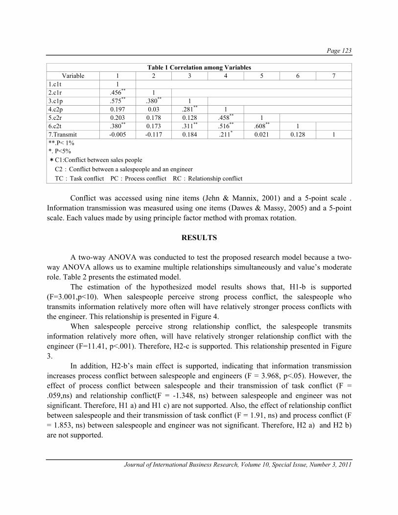
Page 123
Journal of International Business Research, Volume 10, Special Issue, Number 3, 2011
Table 1 Correlation among Variables Variable 1 2 3 4 5 6 7
1.c1t 1 2.c1r .456** 1 3.c1p .575** .380** 1 4.c2p 0.197 0.03 .281** 1 5.c2r 0.203 0.178 0.128 .458** 1 6.c2t .380** 0.173 .311** .516** .608** 1 7.Transmit -0.005 -0.117 0.184 .211* 0.021 0.128 1 **.P< 1% *. P<5% *C1:Conflict between sales people C2:Conflict between a salespeople and an engineer TC:Task conflict PC:Process conflict RC:Relationship conflict
Conflict was accessed using nine items (Jehn & Mannix, 2001) and a 5-point scale . Information transmission was measured using one items (Dawes & Massy, 2005) and a 5-point scale. Each values made by using principle factor method with promax rotation.
RESULTS
A two-way ANOVA was conducted to test the proposed research model because a two-way ANOVA allows us to examine multiple relationships simultaneously and value’s moderate role. Table 2 presents the estimated model. The estimation of the hypothesized model results shows that, H1-b is supported (F=3.001,p<10). When salespeople perceive strong process conflict, the salespeople who transmits information relatively more often will have relatively stronger process conflicts with the engineer. This relationship is presented in Figure 4.
When salespeople perceive strong relationship conflict, the salespeople transmits information relatively more often, will have relatively stronger relationship conflict with the engineer (F=11.41, p<.001). Therefore, H2-c is supported. This relationship presented in Figure 3.
In addition, H2-b’s main effect is supported, indicating that information transmission increases process conflict between salespeople and engineers (F = 3.968, p<.05). However, the effect of process conflict between salespeople and their transmission of task conflict (F = .059,ns) and relationship conflict(F = -1.348, ns) between salespeople and engineer was not significant. Therefore, H1 a) and H1 c) are not supported. Also, the effect of relationship conflict between salespeople and their transmission of task conflict (F = 1.91, ns) and process conflict (F = 1.853, ns) between salespeople and engineer was not significant. Therefore, H2 a) and H2 b) are not supported.
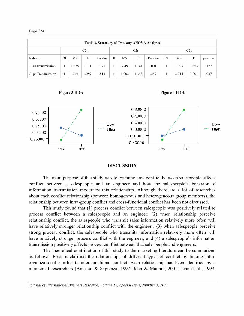
Page 124
Journal of International Business Research, Volume 10, Special Issue, Number 3, 2011
Table 2. Summary of Two-way ANOVA Analysis
C2t C2r C2p
Values Df MS F P-value Df MS F P-value Df MS F p-value
C1r×Transmission 1 1.655 1.91 .170 1 7.49 11.41 .001 1 1.795 1.853 .177
C1p×Transmission 1 .049 .059 .813 1 1.002 1.348 .249 1 2.714 3.001 .087
Figure 3 H 2-c Figure 4 H 1-b
DISCUSSION
The main purpose of this study was to examine how conflict between salespeople affects conflict between a salespeople and an engineer and how the salespeople’s behavior of information transmission moderates this relationship. Although there are a lot of researches about each conflict relationship (between homogeneous and heterogeneous group members), the relationship between intra-group conflict and cross-functional conflict has been not discussed.
This study found that (1) process conflict between salespeople was positively related to process conflict between a salespeople and an engineer; (2) when relationship perceive relationship conflict, the salespeople who transmit sales information relatively more often will have relatively stronger relationship conflict with the engineer ; (3) when salespeople perceive strong process conflict, the salespeople who transmits information relatively more often will have relatively stronger process conflict with the engineer; and (4) a salespeople’s information transmission positively affects process conflict between that salespeople and engineers.
The theoretical contribution of this study to the marketing literature can be summarized as follows. First, it clarified the relationships of different types of conflict by linking intra- organizational conflict to inter-functional conflict. Each relationship has been identified by a number of researchers (Amason & Sapienza, 1997; Jehn & Mannix, 2001; Jehn et al., 1999;

Page 125
Journal of International Business Research, Volume 10, Special Issue, Number 3, 2011
Song & Parry, 1997) , but they have not examined the relationship between the two types of conflict. Although this study did not find all types of conflict to be related, it is clear that process conflict between salespeople increases conflict between a salespeople and an engineer. One explanation of this finding is that process conflict provides an opportunity to solve a problem. Perhaps when salespeople has process conflict with another salespeople, that salespeople want technical knowledge from an engineer to access more resources than the other salespeople and resolve their role uncertainty.
Second, the results show that a salespeople’s information transmission positively affects process conflict between a salespeople and an engineer. Some authors have suggested that process conflict disturbs members’ communication and information sharing (Jehn &Manniz, 2001; Matsuo, 2006). The findings indicate that information sharing activates inter-functional process conflict. One possible explanation for the information transmission/ process conflict relationship is as follows; through information transmission, a salespeople provides a process issue to discuss. For that reason, information transmission may increased process conflict between a salespeople and an engineer.
Finally, the results indicate that information transmission by salespeople moderates the relationship between intra-organizational conflict and inter-functional conflict. In the marketing study, information transmission has been discussed as a method for resolving conflicts (Dawes & Massey, 2005). On the other hand, some research has reported that frequent communication is reason for conflict. In this research, the results suggest that frequent communication positively affects conflict between salespeople and engineer. One possible explanation for the information transmission/ conflict relationship is as follows. Communication might enhance the likelihood of conflict’s occurrence by suggesting own purpose and performance. Souder (1981) pointed out that each function has a different purpose, time-orientation, and method of understanding. Therefore, they take priority over the other peoples’ purpose, leading to conflict. In particular, in this research, the results indicate that when conflict between salespeople is strong, the conflict gap between salespeople and engineer is widened by communication transmission. From these findings, we predict that, when salespeople who have strong conflict transmits sales information, inter-functional conflict will increase.
Therefore, this study has two managerial implications. First, sales managers should note the conflict relationship between salespeople. For sales managers to reduce the conflict between salespeople and engineers, they need to focus on those who have to act boundary spanners transmitting sales information to engineers. By selecting salespeople to transmit sales information to engineers, managers can control conflict.
Second, sales managers should control salespeoples’ process conflict and relationship conflict. Process conflict refers to disagreement about resources and job allocation (Jehn & Mannix, 2001), and relationship conflict means disagreement about interpersonal incompatibilities (Amason & Sapienza, 1997). Since these two negative conflicts positively affect inter-functional negative conflict, conflict between salespeople has to be controlled first.
Page 126
Journal of International Business Research, Volume 10, Special Issue, Number 3, 2011
Sales managers must monitor the conflict situation within the sales department, and participate in managing the conflict relationship while giving advice and solutions to salespeople. It may be crucial for managers to reduce negative conflict within in the company.
REFERENCES Alderfer,C.P & K.K. Smith(1982). Studying intergroup relations embedded in organization, Administrative Science
Quarterly,27(1),35-65. Aldrich,H. & D,Herker(1977). Boundary spanning roles & organization structure. Academy of Management
Review,April,217-230. Amason,A.C. (1996) . Distinguishing the effects of functional and dysfunctional conflict on strategic decision
making: resolving a paradox for top management teams. Academy of Management Journal,39(1),123-148. Amason.A.C. & H. J.Sapienza(1997) .The effect of top management team size and integration norms on congnitive
& affective conflict. Journal of management,23(4),495-516. Bowen, Murray(1978) Family Therapy in Clinical Practice, New York: Jason Aronson. Bulding,K.E. (1963) .Towards a pure theory of threat systems. American Economic Review,53(2),424-434. Crittenden.,V. L.,L.R.Gardiner & Antonie Stam(1993) . Reducing conflict between marketing & manufacturing.
Industrial Marketing Management,22,299-309. Dawes,P.L & G.R.Massey(2005) . Antecedents of conflict in marketing’s cross-functional relationship with sales.
European Journal of Marketing,39(11/12),1327-1344. Dechurch,L.A & M.A.Marks(2001). Maximizing the benefits of task conflict: the role of conflict management. The
International Journal of Conflict Management,12(1),4-22. Dougherty,D(1992) . A practice-centered model of organizational renewal through product innovation. Strategic
Management Journal,13(51),77-92. Dreu,C.K.W.D & L.R.Weingart(2003). Task versus relationship conflict, team performance, and team member
satisfaction: a meta-analysis, Journal of Applied Psychology. 88(4),741-749. Dreu, C.K.W.D (2006). When too little or too much hurts: evidence for a curvilinear relationship between task
conflict & innovation in teams, Journal of Management,32(1).Feburary.83-107. Hunter ,G.L.& D.J.Goebel(2008). Salespersons' information overload: scale development, validation, and its
relationship to salesperson job satisfaction and performance. Journal of Personal Selling and Sales Management,28(1),21-35.
Jehn,K.A(1995) . A multimethod examination of the benefits & detriments of intragroup conflict, Administrative Science Quarterly,40,256-282.
Jehn,K.A(1997). A qualitative analysis of conflict types and dimensions in organizational group, Administrative Science Qualterly,40,256-282.
Jehn,K.A., G.B.Northcraft & M.A.Neale(1999). Why differences make a difference: a field study of diversity, conflict, and performance in workgroups, Administrative Science Quarterly,44,.741-763.
Jehn,K..A & E.A.Mannix (2001). The dynamic nature of conflict; a logtudinal study of intragroup conflict & group performance. Academy of Management Journal,44(2),238-251.
Jehn,K..A , E.A.Mannix-,Northcragr,G.B,Meale,M.A(1999). Why differences make a difference: a field study of divertsity,conflict,& performance in workgroups. Administrative Science Quarterly,44,741-763.
Jehn,K.A & C.Bendersky(2003) . Intragroup conflict in organizations: a contingency perspective on the conflict-outcome relationship. Research in Organizational Behavior,25,187-242.
Kawakami,T & M.Song(2004) . The moderation effect of product innovativeness on the relationship of customer information and new product performance. AMA 2004 Winter Educators’ s Conference Proceedings,15,106-111.

Page 127
Journal of International Business Research, Volume 10, Special Issue, Number 3, 2011
Lovelace,K., D.LShaoiro &L.R.Weingart(2001). Maximizing cross-functional new product teams’ innovativeness and constraint adherence: a conflict communications perspective, Academy of management Journal, 44(4),779-793.
Martz,E & A. K.Kohli(1996). Market intelligence dissemination across functional boundaries. Journal of Marketing Research ,33(1),47-61.
Martz,E & A. K.Kohli -(2000) . Reducing marketing’s conflict with other functions: the differential effects of integrating mechanisms. Journal of the Academy of Marketing Science,28(4),479-492.
M,Matsuo.(2006) .Customer orientation ,conflict ,& innovativeness. Journal of Business Research,59,242-250. Morgan,N.A & N.F.Piercy(1996). Interactions between marketing and quality at the SBU level: influences and
outcomes, Academy of Marketing Science,26(3),190-208. Pelled, L.H., K.M.Eisenhardt , K.R. Xin(1999). Exploring the black box: an analysis of work group diversity,
conflict, and performance. Administrative Science Quarterly,44,1-28. Proudford., Karen L & Kenwyn K Smith(2003). Group Membership Salience and the Movement of Conflict, Group
&Organization Management,28(1),18-44. Schmidt,M.S & T.A.Kochan(1972) . Conflict : Toward conceptual clarity. Administrative science
Qualrterly,17(3),359-370. Schwenk,C.R(1990). Conflict in organizational decision making: an exploratory study of its effect for-profit not
for-profit organizations. Management Science,36(4),436-448. Smith,K.K.(1989). The movement of conflict in organizations; the joint dynamics of splitting and triangulation,
Administrative Science Quarterly,34,1-20. Song,X.M. & M.E.Parry(1997). Teamwork barriers in Japanese high-technology firms: the sociocultural differences
between R&D and marketing managers. Journal of Product Innovation Management ,14(5),365-367. Souder, William E(1981). Disharmony between R&D and Marketing, Industrial Marketing Management,10(1), 67-
73. Tomas,K.M(1978). Conflict and conflict management: reflections and update, Journal of Organizational Behavior,
13(3),265-274. Tushman,M.L,T.J.Scanilan (1981). Boundary spanning individuals: transfer and their role in information transfer
and their antecedents. Academy of Management Journal,24(2),289-305. Xie,J.H.,M.Song, & A. Stringfellow(2003). Antecedents and consequences of goal incongruity on new product
development in five countries: a marketing view. Product Development &Management Association,20,233-250

Page 128
Journal of International Business Research, Volume 10, Special Issue, Number 3, 2011

Page 129
Journal of International Business Research, Volume 10, Special Issue, Number 3, 2011
ARE PHILIPPINE FIXED INCOME FUND MANAGERS GENERATING ALPHA FOR THEIR CLIENTS?
Clive Manuel O. Wee Sit, De La Salle University-Manila
ABSTRACT
The Sharpe, Treynor, Jensen’s alpha, and information ratio portfolio performance measures are widely-used in the asset management industry to appraise investment performance due to their strong foundations in Modern Portfolio Theory, their practical uses in the ranking of investment funds, and their ability to quantify an investment’s realized alpha or degree of investment outperformance relative to a specific benchmark return. This paper is an application of these portfolio performance measures on fixed income investment companies (mutual funds) in the Philippines over a 1-, 3-, and 5-year returns computation horizon, aimed at identifying which portfolio managers are superior in market-timing, securities selection, and in the use of new information to generate excess or abnormal returns on their fixed income funds after having accounted for risk.
INTRODUCTION Mutual funds, also known as investment companies, are pooled investment vehicles managed by an asset management firm that seeks to create value for shareholders through tactical allocation of investor funds in various asset classes or in securities within a particular asset category. Typically, mutual funds are classified based on investment style, and can be broadly identified as either a fixed income fund, an equity fund, or a balanced fund (combination of fixed income and equity instruments), depending on the specific assets the fund is allowed to invest in (as stated in the fund’s prospectus). Investors consider mutual funds to be a viable alternative to direct investments in equity and debt securities due to a number of benefits that can be derived from pooled fund-investing, which include, but are not limited to, easy liquidity, economies-of-scale, access to otherwise inaccessible markets, diversification, and management of funds by a skilled and knowledgeable investments practitioner. For an asset management firm to act as fund manager and administrator of an investment company, it must be awarded a management and distribution mandate by fund participants (owners). Mandated asset managers are expected to perform the following basic duties in exchange for a periodic management fee: distribute shares in the fund to potential investors, provide ready liquidity to clients who wish to divest their existing mutual fund holdings, act as investment advisor and administrator to the investment company, and manage the fund’s securities portfolio for the collective benefit of all fund shareholders. However, asset managers

Page 130
Journal of International Business Research, Volume 10, Special Issue, Number 3, 2011
are scrutinized by the investing community on the basis of their ability to generate returns not just relative to competitors but vis-à-vis a chosen benchmark portfolio as well. Since ownership in a mutual fund is dispersed given its pooled nature, the interests of the majority shareholders of the fund, just like in any registered corporation, are represented by a board of directors. And one of the key responsibilities of the board of directors is to prudently select a fund manager and periodically evaluate its performance in all of the five aforementioned aspects, with returns relative to peers and benchmark being one of the more critical aspects in determining investment success for the client. Asset managers that exhibit more than just modest performance are likely to have their mandate as fund manager renewed during each periodic review by the board of directors. This process of performance measurement and evaluation ensures that fund managers remain competitive in the pooled fund investments industry. Mutual Fund Industry Growth in the Philippines To put the competitive landscape of mutual fund investments in proper perspective, assets under management (AUM) in the Philippine mutual fund industry reached a historic high of PHP 95.7-billion as of the end of 2010. This is a dramatic increase from the PHP 1.35-billion AUM of managers of local mutual funds back in 1997 (Valderrama & Bautista, 2003). Of the PHP 95.7-billion, 19.8% represents investments in funds whose main investment style is long-term growth through equity investments, 58.3% is in the form of funds invested purely in short-term to long-term fixed income instruments, and the remaining 21.9% is allocated in balanced portfolios of both stocks and bonds (balanced fund category). In terms of number of players in the industry, the number of mutual funds in the Philippines has grown from 25 in the year 2003 to 45 in 2010, evidence to the intensifying competitive structure of the local pooled investments industry. The sudden surge of unit investment trust funds (UITFs) beginning 2005 due to the phase-out of common trust funds (CTFs) by the Bangko Sentral ng Pilipinas (BSP) likewise facilitated the rise in competition between fund managers, not to mention the improvement in domestic macroeconomic and financial market conditions since 2005 which increased demand for pooled investments. As of the end of December 2010, there were 79 UITFs operated by 16 trust departments of banks. This compares to the 10 asset management firms that provide advisory and management services to mutual funds. Philippine Fixed Income Mutual Funds It is notable that fixed income funds are the preferred investment avenue among Philippine mutual fund shareholders. And this is not at all unexpected given the relatively conservative profile of most Filipino investors. However, it is also noteworthy that the fraction of the mutual fund industry’s AUM accounted for by fixed income funds (58.3% in December 2010) has fallen considerably from the 92.2% recorded in 2002 (Valderrama & Bautista, 2003).

Page 131
Journal of International Business Research, Volume 10, Special Issue, Number 3, 2011
The decline in the share of fixed income funds in the net assets of the mutual fund sector can be attributed to the marked improvement in the performance of the Philippine stock market in recent years and the migration from accrual to mark-to-market accounting for fixed income funds in 2005, which created more volatility in the local fixed income industry. Notwithstanding the drop in AUM share of fixed income funds among the investment companies, the number of fixed income mutual funds continued to grow from the 4 bond funds recorded in the year 2000 to the 26 different types of fixed income funds in 2010. Of this 26, 10 are in the form of Peso-denominated bond funds, 9 are in Dollar-denominated bond funds, 2 are Euro-denominated bond funds, while 5 are Peso-denominated money market funds. The recent launch of global bond funds by some of the bigger players in the industry suggests that there is demand potential for fixed income funds in the Philippines. Objectives of the Study In view of the stiff competition and growth prospects of mutual funds in the pooled investments plane, it is clear that an objective and relative measure of fund manager ability is imperative to give clients a means of assessing whether or not the fund managers these clients have mandated to help them reach their investment goals are indeed performing up to par with expectations. The goal of this research undertaking is to quantitatively appraise the risk-adjusted returns performance of managers of mutual funds in the Philippines, specifically those that have been contracted by their clients to manage a fixed income portfolio on their behalf. The study will look at the more commonly-watched parameters of mutual fund performance used by industry practitioners to be able to ascertain how effective Philippine fixed income fund managers are in utilizing available information and in taking advantage of market opportunities to further the returns performance of their managed portfolios. These composite portfolio performance measures are the Sharpe ratio, the Treynor ratio, the Jensen’s alpha measure, and the information ratio. These metrics shall be applied to the historical returns of Philippine mutual funds over a 1-, 3-, and 5-year computation horizon to determine whether fund managers of fixed income funds are consistently providing returns beyond what is expected of them on a risk-adjusted basis and to establish which among these asset management firms consistently perform better than their peers and benchmark.
DESIRABLE ATTRIBUTES OF PORTFOLIO MANAGERS There are two primary characteristics that investors seek from their portfolio managers. First is a fund manager’s ability to generate above-average returns for a given risk profile. Superior returns can be attained if a fund manager has the ability to properly time the market and has the skill of identifying and trading incorrectly priced securities in the market. The former can be seen in a fund manager of a fixed income portfolio who increases the duration of his bond

Page 132
Journal of International Business Research, Volume 10, Special Issue, Number 3, 2011
holdings prior to an anticipated drop in interest rates and decreases duration when he expects yields to rise. Such a market-timing strategy, if implemented properly, would make his fixed income portfolio valuations more sensitive to falling interest rates (have more bond price appreciation) and more defensive to rising interest rates (less bond price depreciation), hence, providing above-average returns for clients. The latter strategy of exploiting asset mispricing would likewise generate above-average returns, most especially if the portfolio manager is able to select undervalued securities for the portfolio (Reilly & Brown, 2009). The second desired attribute is a fund manager’s ability to rid a securities portfolio of all unnecessary unsystematic risks by virtue of diversification. This implies that investors in general would prefer to have their funds invested in a completely diversified portfolio of securities because they do not expect to be compensated for unsystematic risks. And the level of diversification of a portfolio relative to a benchmark or market index is measured by the correlation of its returns to the said market index. The relevance of these two portfolio manager attributes is that some portfolio performance assessment tools only consider one of the two characteristics while others indirectly consider both but fail to differentiate them (Reilly & Brown, 2009).
EARLY PORTFOLIO PERFORMANCE MEASUREMENT TECHNIQUES
Prior to the extensive work on portfolio theory in the 1960s, most investors evaluated investments solely on the basis of returns without explicitly accounting for risk. Although Modern Portfolio Theory introduced the concept of risk as the volatility of investment returns, analysts back in the 1960s would consider returns and risk as two separate and distinct realities and would make comparisons of portfolios within a particular risk class (those with similar returns variability). Portfolio analysts would group pooled funds together, not on the basis of investment style, but on the basis of variability of returns. This meant that funds that had similar returns variability would be categorized within the same peer group and pitted against one another to determine which fund generated the highest returns within the sample notwithstanding the fact that these funds may be invested in different asset classes. For example, a portfolio of high-yield corporate bonds could actually be grouped with a portfolio of equities with a totally different investment style and categorized within the same peer group just because they exhibit similar returns variability. An obvious problem to peer group comparisons such as these that only look at returns is that it disregards varying investment styles of fund managers and makes it difficult for investors to determine whether fund managers have met their clients’ investment objectives after having satisfied certain investment constraints (Reilly & Brown, 2009).

Page 133
Journal of International Business Research, Volume 10, Special Issue, Number 3, 2011
COMPOSITE MEASURES OF PORTFOLIO PERFORMANCE Some of the shortcomings of early portfolio performance assessment tools were the fact that they were very returns-centric and failed to properly account for risk. These shortfalls were a result of the lack of literature in portfolio theory during the time that combined both return and risk in performance appraisal. After the development of the Capital Asset Pricing Model (CAPM) by Sharpe, Treynor, and Mossin, in the 1960s, investors and financial economists alike recognized the need to address the issue of adjusting for risk in investment performance evaluation, which led to the development of a number of extensions to the CAPM. Three measures were proposed in the finance literature to account for risk when assessing portfolio returns--these are the Treynor, Sharpe, and Jensen portfolio performance measures, which are most commonly referred to as the composite measures of portfolio performance. Each method attempts to quantify a mutual fund’s performance relative to a risk-adjusted return appropriate for a portfolio of the same risk. A portfolio’s returns performance is deemed successful when it yields a return better than the benchmark equilibrium return (Chua, et al., 2008). Treynor Portfolio Performance Measure Jack Treynor in 1965 developed the first composite portfolio performance measure that included risk. The two components of risk he considered are the risk from general fluctuations in market returns and the risk from idiosyncratic fluctuations of securities in a portfolio. He proposed that all portfolios have a unique characteristic line that defines its degree of sensitivity to the returns on a market (benchmark) portfolio. The slope of the characteristic line is also known as beta and is a direct measure of a portfolio’s relative risk attributes. Portfolios with beta coefficients equal to 1.0 have a risk that exactly mimics that of a market portfolio assumed to be fully diversified (with no unique risk). He developed the Treynor measure because of his desire to introduce a performance parameter that could be utilized by all investors irrespective of their risk profiles. Building on the assumptions of Capital Market Theory, a risk-free asset is bundled with different portfolios to form a portfolio possibility line. Risk-averse investors would always prefer the portfolio possibility line with the highest slope since this would maximize an investor’s return in excess of the risk-free rate for every unit of market risk. The Treynor ratio, denoted as Ti, is also known as the reward-to-volatility ratio and is the slope of the portfolio possibility line that rational investors seek to maximize. This is given in Equation (1).
(1)

Page 134
Journal of International Business Research, Volume 10, Special Issue, Number 3, 2011
In this expression, Ri is the average rate of return for portfolio i, RFR is the risk-free rate of return, and Ri is the slope of the characteristic line during a specific time period. The numerator of this ratio is a risk premium that captures the extra return an investor earns from the portfolio during a specified time period over and above the return on a simple buy-and-hold strategy on a risk-free asset with a similar holding period. The denominator of this ratio, meanwhile, is a proxy for the portfolio’s risk as captured by its beta coefficient, which measures only systematic risk. Treynor’s rationale for using beta (and not total risk) as the relevant proxy for uncertainty is his assumption that investors do not require compensation for bearing unique risks that can be eliminated by investing in a completely diversified portfolio (which is the benchmark that investors and fund managers attempt to beat in terms of risk-adjusted returns). Putting returns and risk together, the Treynor ratio quantifies a portfolio’s risk premium return per unit of risk (Reilly & Brown, 2009). A high and positive Treynor ratio shows superior risk-adjusted performance for a fund, whereas a low and negative Treynor ratio may be indicative of unfavorable performance (Chua, et al., 2008). Plotting the Treynor ratios of a series of portfolios (including the market portfolio) on a graph allows investors to ascertain whether each portfolio is located above or below the Security Market Line (SML), which is a line that links the risk-free asset with the market portfolio and has a beta of 1.0. Such an exercise would facilitate investment analysis and aid investors in visually determining a portfolio’s outperformance relative to peers and the market on a risk-adjusted basis. It must be noted however that the Treynor portfolio performance measure is a ranking criterion for mutual funds and provides relative, but not absolute, rankings of portfolios. Portfolios that plot higher than the SML, and hence, have a higher reward-to-volatility ratio relative to the market portfolio, have generated alpha for their clients, or risk-adjusted returns greater than that of the benchmark (Reilly & Brown, 2009). One problem with the use of the Treynor measure is its use of beta as its measure of risk. Estimating a portfolio’s beta coefficient using regression may introduce estimation bias because of the assumption that beta is constant over a specific period of investigation. An alternative method of arriving at the beta coefficient, which is a portfolio’s covariance of returns with the market divided by the variance of the market’s returns during a particular estimation period, shall be used for the purposes of this study. Sharpe Portfolio Performance Measure Just a year after Treynor introduced the first composite measure of portfolio performance, William Sharpe in 1966 proposed another method of evaluating the performance of mutual funds as an offshoot to his previous work on the CAPM and Capital Market Theory. The Sharpe ratio is similar to the Treynor measure in that it also quantifies reward-to-variability. But instead of considering only the risk of a portfolio relative to that of a fully diversified basket of assets, Sharpe sought to measure risk-adjusted performance by looking at a portfolio’s total risk, which

Page 135
Journal of International Business Research, Volume 10, Special Issue, Number 3, 2011
considers both market risks and risks specific or unique to the underlying assets in a portfolio. The proxy for risk he suggested was a measure of dispersion of a portfolio’s returns series from its mean value, also known as a portfolio’s standard deviation of returns. Similar to Treynor’s measure of excess returns, Sharpe utilized the same definition, which is the incremental return on a portfolio during a specified time horizon over and above the return on a passive investment in a risk-free asset over a similar time frame. The Sharpe ratio, denoted by Si, is therefore a portfolio’s risk premium return earned per unit of total risk (Reilly & Brown, 2009). This is given in Equation (2).
(2)
In addition to the earlier notation, σi is the standard deviation of the return of portfolio i during the time period being analyzed.
The evaluation criteria for the Sharpe measure does not deviate much from Treynor’s methodology. A higher Sharpe ratio is desired for a portfolio since this would suggest that a fund manager was able to generate incrementally higher excess returns for every unit of total risk. Sharpe’s use of standard deviation of returns as the relevant risk measure makes Capital Market Theory the theoretical basis for comparing portfolio performance (compared to the CAPM for Treynor’s measure). Combining a risk-free asset with different risky investment portfolios (whose total risk is defined by its standard deviation of returns) results in portfolio combinations that plot above, below, or along the Capital Market Line (CML). Mutual funds that plot above the CML are considered superior to the market portfolio in the sense that they provide shareholders with an excess return higher than the benchmark on a risk-adjusted basis (Reilly & Brown, 2009). These pooled funds are considered alpha-generating due to their benchmark outperformance. Portfolios with a higher reward-to-variability ratio relative to peers likewise exhibit returns outperformance vis-à-vis competitors after accounting for total risk. It must be noted, however, that the Sharpe measure, just like the Treynor ratio, is a relative, and not absolute, measure of portfolio success. The use of Sharpe ratios can likewise facilitate a ranking of investment funds. The widespread use of the Sharpe ratio in the investments industry comes from its simplicity and straightforwardness. Its use of total risk makes the risk-adjustment process less dependent on stringent assumptions (such as the implicit presumption of full diversification for the Treynor ratio). Jensen Portfolio Performance Measure In 1968, Jensen proposed an extension to the CAPM that would address the inability of the Sharpe and Treynor portfolio metrics to quantify the investment ability of a portfolio

Page 136
Journal of International Business Research, Volume 10, Special Issue, Number 3, 2011
manager on an absolute basis. He postulated that a fund manager’s unique skill in forecasting market turns and selecting undervalued securities for his portfolio can be measured empirically by analyzing a portfolio manager’s alpha coefficient. The alpha coefficient, symbolically represented by (αj) is the portion of a portfolio’s excess return (over the risk-free rate) that is beyond the market risk premium required or expected from an investment based on an equilibrium asset pricing model such as the CAPM or a multi-factor model of risk and return such as the Arbitrage Pricing Theory (APT). A portfolio manager is deemed to have outperformed his benchmark if the Jensen’s alpha is positive and statistically significant (Reilly & Brown, 2009). To arrive at Jensen’s alpha coefficient, the basic CAPM expression, assuming it is empirically valid, is extended by deducting both sides of the equation by the risk-free rate of return. This would result in the following regression model given in Equation (3):
(3) where Rjt is the realized return on portfolio j over a given period, RFRt is the one-period risk-free interest rate, Rj is the systematic risk for portfolio j, and Rmt is the return on the market portfolio over the same holding period as portfolio j. If the market were in equilibrium, an intercept (alpha) would no longer be expected. But if fund managers are anticipated to provide investors with superior returns due to market timing and security selection skills, a non-zero intercept (alpha) must be introduced in the regression model that would capture this unique skill of portfolio managers. A statistically significant positive (negative) alpha is reflective of a fund manager’s superior (inferior) abilities. The regression model that incorporates the intercept (alpha coefficient) is given in Equation (4):
(4) Rearranging Equation (4) results in the Jensen’s alpha equation that measures a fund manager’s absolute degree of outperformance (underperformance) relative to a benchmark’s expected return required by a pricing model, as given in Equation (5).
(5) Although Jensen’s portfolio performance measure addresses the need for some analysts to quantify absolute performance of mutual funds, it is not without its share of shortcomings. It must be noted that the use of regression to estimate the value of Jensen’s alpha may make it subject to statistical biases. Moreover, Jensen’s alpha is sensitive to the choice of benchmark (CAPM or APT) and estimation method for calculating beta (Chua, et al., 2008). For this study,

Page 137
Journal of International Business Research, Volume 10, Special Issue, Number 3, 2011
the proponent has elected to calculate beta for the Jensen’s alpha measure using the same estimation method implemented in obtaining the systematic risk component of the Treynor ratio. For the choice of benchmark in Jensen’s alpha, the single-factor CAPM shall be utilized to arrive at a portfolio’s market risk premium. Information Ratio Performance Measure A fourth composite measure of portfolio performance that is widely used in the asset management industry is the information ratio, which is a risk-adjusted performance statistic that takes the return on a managed portfolio in excess of the returns on a benchmark portfolio and divides this by the standard deviation of this excess return. The numerator of the formula represents a fund manager’s ability to use his professional asset management skills and information or knowledge of the markets to generate incremental returns over and above the benchmark clients use to assess his performance. The denominator, meanwhile, measures the amount of unsystematic risk the investors are exposed to because of the fund manager’s active portfolio management efforts in pursuit of those excess returns (Reilly & Brown, 2009). This standard deviation of excess returns due to active management is also known as the tracking error. In notation form, the information ratio, denoted by IRj , is expressed in Equation (6):
(6)
where Rb is the average return for the benchmark portfolio during the period and σER is the standard deviation of the excess return during the period. The information ratio is an example of a benefit-to-cost ratio because the tracking error is the cost of active portfolio management with the excess return of the portfolio relative to the market being the reward that is due to investors resulting from the portfolio manager’s decision to deviate from a passive market benchmark portfolio-tracking strategy. Just as in both Treynor and Sharpe’s measures, a higher information ratio is desired because it shows that a fund manager has maximized his active portfolio management skills to create value for his clients on a risk-adjusted basis. The information ratio has its similarities to the three previously discussed portfolio performance metrics and can be considered a combination of the three. It is similar to the Sharpe and Treynor measures in that it is also a risk-adjusted measure of return that highlights a portfolio’s relative, and not absolute, performance. The information ratio has a more noticeable similarity to the Sharpe ratio because of its use of standard deviation of returns as its proxy for uncertainty. Comparing the information ratio to the Jensen’s alpha measure, it somewhat
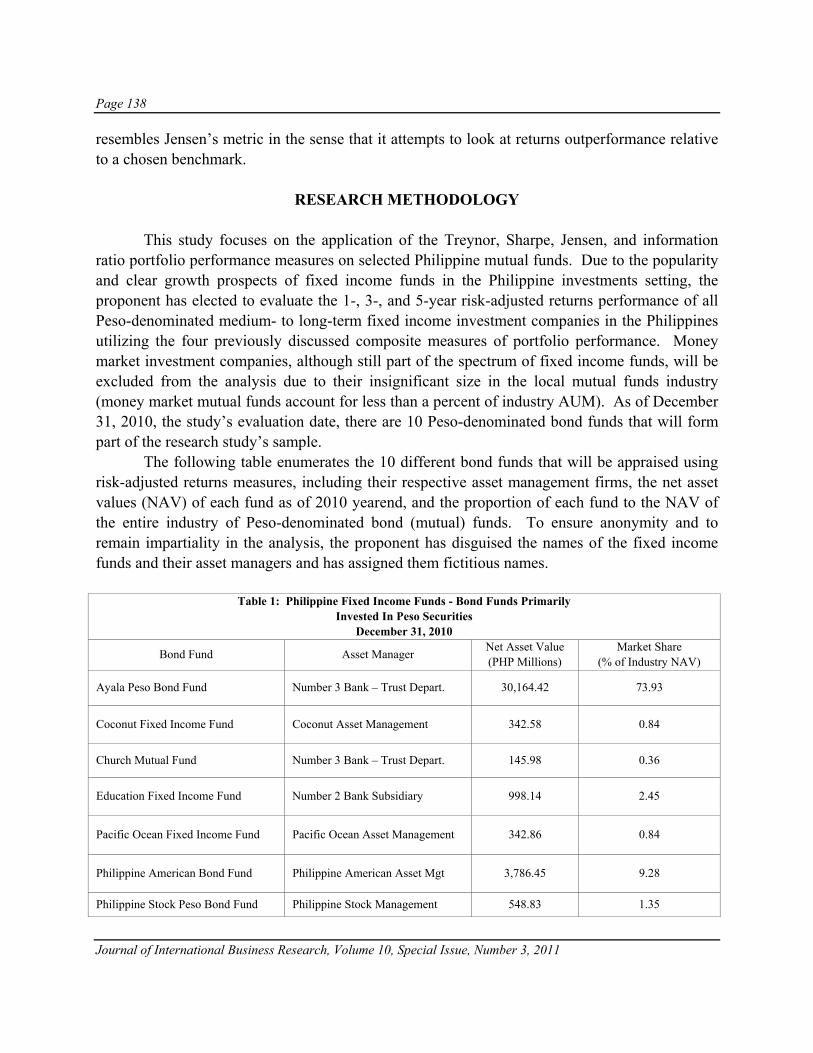
Page 138
Journal of International Business Research, Volume 10, Special Issue, Number 3, 2011
resembles Jensen’s metric in the sense that it attempts to look at returns outperformance relative to a chosen benchmark.
RESEARCH METHODOLOGY This study focuses on the application of the Treynor, Sharpe, Jensen, and information ratio portfolio performance measures on selected Philippine mutual funds. Due to the popularity and clear growth prospects of fixed income funds in the Philippine investments setting, the proponent has elected to evaluate the 1-, 3-, and 5-year risk-adjusted returns performance of all Peso-denominated medium- to long-term fixed income investment companies in the Philippines utilizing the four previously discussed composite measures of portfolio performance. Money market investment companies, although still part of the spectrum of fixed income funds, will be excluded from the analysis due to their insignificant size in the local mutual funds industry (money market mutual funds account for less than a percent of industry AUM). As of December 31, 2010, the study’s evaluation date, there are 10 Peso-denominated bond funds that will form part of the research study’s sample. The following table enumerates the 10 different bond funds that will be appraised using risk-adjusted returns measures, including their respective asset management firms, the net asset values (NAV) of each fund as of 2010 yearend, and the proportion of each fund to the NAV of the entire industry of Peso-denominated bond (mutual) funds. To ensure anonymity and to remain impartiality in the analysis, the proponent has disguised the names of the fixed income funds and their asset managers and has assigned them fictitious names.
Table 1: Philippine Fixed Income Funds - Bond Funds Primarily Invested In Peso Securities
December 31, 2010
Bond Fund Asset Manager Net Asset Value (PHP Millions)
Market Share (% of Industry NAV)
Ayala Peso Bond Fund Number 3 Bank – Trust Depart. 30,164.42 73.93
Coconut Fixed Income Fund Coconut Asset Management 342.58 0.84
Church Mutual Fund Number 3 Bank – Trust Depart. 145.98 0.36
Education Fixed Income Fund Number 2 Bank Subsidiary 998.14 2.45
Pacific Ocean Fixed Income Fund Pacific Ocean Asset Management 342.86 0.84
Philippine American Bond Fund Philippine American Asset Mgt 3,786.45 9.28
Philippine Stock Peso Bond Fund Philippine Stock Management 548.83 1.35

Page 139
Journal of International Business Research, Volume 10, Special Issue, Number 3, 2011
Table 1: Philippine Fixed Income Funds - Bond Funds Primarily Invested In Peso Securities
December 31, 2010
Bond Fund Asset Manager Net Asset Value (PHP Millions)
Market Share (% of Industry NAV)
Prudence Fixed Income Fund German Bank – Trust Depart. 287.94 0.71
Sunshine Bond Fund Sunshine Asset Management 3,290.29 8.06
Sunshine GS Fund Sunshine Asset Management 895.94 2.20
Returns performance will be analyzed using a 1-, 3-, and 5-year time horizon since this is the convention used by most asset managers in presenting historical fund performance. 1-year rolling returns shall be computed by taking the year-over-year percentage change in the Net Asset Value Per Share (NAVPS) of a mutual fund or portfolio during the last day of each month beginning January 2010 until December 31, 2010, the study’s evaluation date, for a total of 12 monthly rolling returns. 3- and 5-year rolling returns, meanwhile, will be calculated in a similar manner by taking the percentage change in a mutual fund’s NAVPS over a 3- and 5-year period respectively. Both the 3- and 5-year rolling returns will have 12 observations each covering the same monthly period of January to December 2010. To ensure that all returns figures are consistently presented in per annum terms, the 3- and 5-year rolling returns will be annualized by using a compound annual growth rate formula. Since all composite returns measures discussed in the previous section require the use of an average of realized portfolio returns, the arithmetic average of the 1-, 3-, and 5-year rolling mutual fund returns over the 12-month period from January to December 2010 will be calculated, and these arithmetic averages shall proxy for average portfolio returns. All official NAVPS data shall be obtained from the website of the local mutual funds association. Because three of the composite portfolio measures that will be studied in this research paper analyze returns performance by considering average mutual fund and benchmark returns in excess of the returns on a risk-free asset, the yield on Peso-denominated Philippine government securities shall substitute for the risk-free rate. To maintain comparability and consistency in the analysis, the tenor of the risk-free asset will be commensurate with the computation horizon or holding period of the portfolio in scrutiny. For example, if the rolling returns of a mutual fund are being investigated over a 1-year evaluation horizon, then the risk-free rate that will be applied to calculate the portfolio’s excess returns will be the fixing yield on a Philippine T-Bill exactly a year prior to the returns computation date. A positive excess return would then imply that investing in the mutual fund over the past year yielded a client a realized return greater than that of a passive investment in a 1-year T-Bill. For the 3- and 5-year portfolio returns evaluation, the fixing yield-to-maturity on a 3- and 5-year Philippine Fixed Rate Treasury Note (FXTN)

Page 140
Journal of International Business Research, Volume 10, Special Issue, Number 3, 2011
exactly 3- and 5-years prior to the returns computation date respectively, will be utilized as the proxy for the risk-free rate. And similar to the process used to calculate average portfolio returns, the arithmetic mean of the 1-, 3-, and 5-year fixing yields over the 12 monthly periods from January to December 2010 shall represent the average risk-free rate of return. For all T-Bill and FXTN yields used, the rates shall be obtained from the website of the Philippine Dealing and Exchange Corporation (PDEx), the operator of the local fixed income exchange. Three risk proxies have been introduced in this research undertaking, each having its own specific function in the risk-assessment process. For the Treynor ratio, which looks solely at a mutual fund’s systematic risk component, quantification of uncertainty is achieved by calculating a fund’s beta coefficient, which is simply the covariance of the return of the portfolio relative to the market divided by the covariance of the market’s returns with itself. The most widely-used and accepted benchmark for the market portfolio by Philippine fixed income fund managers is the HSBC Philippines Local Currency Government Bond Total Return Index. This index is normally used as the benchmark for Peso-denominated fixed income funds primarily invested in medium- to long-duration government securities. The proponent has chosen not to compute beta using regression analysis to overcome potential problems of statistical bias and model misspecification during estimation. A mutual fund’s beta aptly describes the linear co-movement of its returns to that of the HSBC Philippines Local Currency Bond Total Return Index and represents the sensitivity of the mutual fund’s returns to changes in the said market index. Operationally, the beta of a mutual fund’s rolling returns with respect to the benchmark index shall be computed by utilizing the rolling returns data of both the mutual fund and the HSBC benchmark over the most recent 12 months immediately prior to the study’s evaluation date. Historical data on the HSBC Philippines Local Currency Bond Total Return Index shall be sourced from Bloomberg, LP. Similar to the Treynor measure, the Jensen’s alpha performance metric utilizes the beta coefficient in accounting for risk in the assessment of returns outperformance. Specifically, the beta is a necessary input in the determination of the required return implied by an asset pricing model that fund managers attempt to hurdle to generate alpha. The same beta coefficients computed for the Treynor measure will be used to quantify alpha based on Jensen’s methodology. Although Jensen prescribes the use of regression when estimating a fund manager’s alpha, for the purposes of this study, the proponent shall calculate alpha simply by taking the difference between the excess return of a mutual fund over and above the required risk premium return implied by the CAPM. Both the Sharpe and information ratio performance assessment methodologies use a different approach to quantifying returns uncertainty when compared to Treynor’s and Jensen’s metrics. Instead of focusing on just the non-diversifiable portion of a portfolio’s returns, the Sharpe and information ratios look at overall risk and unsystematic risk respectively in accounting for variability in mutual fund returns. Particularly, Sharpe operationalizes risk quantification in a mutual fund portfolio by computing for the standard deviation of its historical
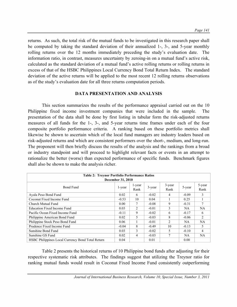
Page 141
Journal of International Business Research, Volume 10, Special Issue, Number 3, 2011
returns. As such, the total risk of the mutual funds to be investigated in this research paper shall be computed by taking the standard deviation of their annualized 1-, 3-, and 5-year monthly rolling returns over the 12 months immediately preceding the study’s evaluation date. The information ratio, in contrast, measures uncertainty by zeroing-in on a mutual fund’s active risk, calculated as the standard deviation of a mutual fund’s active rolling returns or rolling returns in excess of that of the HSBC Philippines Local Currency Bond Total Return Index. The standard deviation of the active returns will be applied to the most recent 12 rolling returns observations as of the study’s evaluation date for all three returns computation periods.
DATA PRESENTATION AND ANALYSIS This section summarizes the results of the performance appraisal carried out on the 10 Philippine fixed income investment companies that were included in the sample. The presentation of the data shall be done by first listing in tabular form the risk-adjusted returns measures of all funds for the 1-, 3-, and 5-year returns time frames under each of the four composite portfolio performance criteria. A ranking based on these portfolio metrics shall likewise be shown to ascertain which of the local fund managers are industry leaders based on risk-adjusted returns and which are consistent performers over the short-, medium, and long-run. The proponent will then briefly discuss the results of the analysis and the rankings from a broad or industry standpoint and will proceed to highlight relevant facts or events in an attempt to rationalize the better (worse) than expected performance of specific funds. Benchmark figures shall also be shown to make the analysis richer.
Table 2: Treynor Portfolio Performance Ratios December 31, 2010
Bond Fund 1-year 1-year Rank 3-year 3-year
Rank 5-year 5-year Rank
Ayala Peso Bond Fund 0.02 6 -0.02 4 -0.09 3 Coconut Fixed Income Fund -0.53 10 0.04 1 0.25 1 Church Mutual Fund 0.00 7 -0.08 9 -0.31 7 Education Fixed Income Fund 0.03 2 -0.01 3 NA NA Pacific Ocean Fixed Income Fund -0.11 9 -0.02 6 -0.17 6 Philippine American Bond Fund 0.02 5 -0.03 8 -0.06 2 Philippine Stock Peso Bond Fund 0.06 1 -0.01 2 NA NA Prudence Fixed Income Fund -0.04 8 -0.49 10 -0.13 5 Sunshine Bond Fund 0.03 3 -0.02 5 -0.10 4 Sunshine GS Fund 0.02 4 -0.03 7 NA NA HSBC Philippines Local Currency Bond Total Return 0.04 0.01 0.00 Table 2 presents the historical returns of 10 Philippine bond funds after adjusting for their respective systematic risk attributes. The findings suggest that utilizing the Treynor ratio for ranking mutual funds would result in Coconut Fixed Income Fund consistently outperforming

Page 142
Journal of International Business Research, Volume 10, Special Issue, Number 3, 2011
competition utilizing 3- and 5-year risk-adjusted returns as bases. Philippine Stock Peso Bond Fund was likewise one of the top performers using the Treynor criterion having been the best bond fund over the 1-year horizon and the 2nd top fund in the 3-year category. Education Fixed Income Fund similarly provided its investors with competitive risk-adjusted rates of return over a 1-year and 3-year returns evaluation time frame, being 2nd and 3rd respectively in terms of ranking.
The perennial underperformers in the industry are those bond funds whose rankings based on risk-adjusted returns are persistently in the 3rd and 4th quartile of performance and at the same time fail to beat the HSBC benchmark over the three returns evaluation periods. These underperformers are Church Mutual Fund and Pacific Ocean Fixed Income Fund. To some extent, Prudence Fixed Income Fund can be considered a laggard as well due to its 1- and 3-year returns both being in the 4th quartile of performance, but then it managed to get into the 2nd quartile for the 5-year returns.
It is also quite apparent from the Treynor ratios computed that with the exception of Coconut Fixed Income Fund, all other bond funds had negative Treynor ratios for the 3- and 5-year periods. Breaking down the Treynor ratios of the funds into their component parts would show that all these funds with negative Treynor metrics had 3- and 5-year average rolling returns that failed to beat on average a passive investment in 3- and 5-year FXTNs respectively. Hence, the underperformance was driven mostly by negative excess returns. The difficulty of most fund managers in exceeding the yield on 3- and 5-year FXTNs comes from the fact that interest rates 3- and 5-years ago, which form the basis for computing the average risk-free rate for 3- and 5-year excess returns, were relatively higher during the time. The underperformance can also be attributed to the effect of a high base in the calculation of portfolio returns. The 3-year rolling returns formula utilizes the months of January to December 2007 as the base months in calculation while the 5-year rolling returns has the months of January to December 2005 as the computational base months. 2005 and 2007 were both relatively good years in the domestic fixed income market, which made NAVPS values of many fixed income funds already high to begin with during these years. 2005 was the final year local fixed income bonds funds were allowed to use accrual accounting as the valuation method for government securities. Because secondary market interest rates in 2005 were trending upward initially due to perceived fiscal risks, government securities were being issued at high rates during the auctions. Since bonds were not being marked-to-market then, fixed income funds were simply accruing the high coupons on the securities they held and were not booking any unrealized losses. Come the end of 2005, interest rates had fallen, and when investments funds were required by the new accounting standards to restate their accrual portfolios in favor of mark-to-market valuation, bond funds immediately realized gains during the migration. This led to 5 out of 9 bond funds having a full-year return that was in double-digit levels. 2007, on the other hand, was the year immediately preceding the global financial crisis. Asset valuations for both the equity and fixed

Page 143
Journal of International Business Research, Volume 10, Special Issue, Number 3, 2011
income markets in the Philippines were elevated and brought about high NAVPS values for equity and bond funds alike.
One of the more interesting findings from the study is the fact that only Coconut Fixed Income Fund and Philippine Stock Peso Bond Fund have historically outperformed the HSBC benchmark using the Treynor ratio as the performance metric. For 1-year returns, only Philippine Stock Peso Bond Fund managed to provide systematic risk-adjusted returns higher than the HSBC benchmark. Whereas for the 3- and 5-year returns, only Coconut Fixed Income Fund’s characteristic line had a slope that is steeper (hence, a higher risk-adjusted return) than the benchmark. This finding implies that only a minority of Philippine asset managers of fixed income investment companies has been beating their benchmark using market risk as the basis for risk-adjusting their returns.
One must exercise caution, however, when coming to the hasty conclusion that based on the Treynor ratio, Coconut Fixed Income Fund has successfully outperformed the HSBC benchmark. Its returns betas for the 1-, 3-, and 5-year returns are -0.12, 0.48, and -0.10 respectively. These negative and low betas imply that the fund’s portfolio manager may have opted to go into asset exposures that are not completely captured by the HSBC index as a performance benchmark. After a thorough investigation of Coconut Fixed Income Fund’s asset allocation as of the end of December 2010, it was discovered that this fund is heavily invested in loans (approximately 91% of the fund’s NAV), which is not subject to daily mark-to-market revaluation, but rather, generates returns by way of accrual income. This significant allocation to loans may explain the low betas. One important takeaway from this is that the HSBC index may not necessarily be an appropriate performance benchmark for Coconut Fixed Income Fund given its bias towards loan exposures (the index construction/rebalancing criteria of the HSBC Philippines Local Currency Bond Total Return Index do not have a provision for loans). This digression in asset allocation from the index may create comparability issues when evaluating mutual fund performance vis-à-vis the benchmark. Although the risk-adjustment process of the Treynor ratio allows for funds with different styles and investment objectives to be pitted against one another, one must first dig deeper into the portfolio composition of the fund to ascertain its comparability with the benchmark before generalizing that it has indeed outperformed its benchmark after controlling for risk.
Another problem when using the Treynor ratio for appraising mutual funds against a benchmark is that negative betas may lead to incorrect conclusions about risk-adjusted performance. Case-in-point is the 1-year Treynor ratio of Coconut Fixed Income Fund of -0.53, which makes it the worst-performing mutual fund in the sample for this specific time horizon (underperforming the HSBC benchmark as well). This is surprising given that its 3- and 5-year Treynor ratios are both the highest among local bond funds and are better than the benchmark for the same time periods. In fact, looking at the returns alone of Coconut Fixed Income Fund (without any risk-adjustment) for the 1-year time horizon shows that it the best performing fund returns-wise. Indeed, it is the negative beta (-0.12) that deflates the risk-adjusted returns of the

Page 144
Journal of International Business Research, Volume 10, Special Issue, Number 3, 2011
fund and complicates the analysis. Reilly & Brown (2009) suggest that when evaluating the performance of a mutual fund with a negative beta, it may be a better approach to compare the realized portfolio return of the fund with its required return based on the CAPM. Implementing this technique would yield a CAPM required return of 2.59%. And since the realized 1-year average rolling return of Coconut Fixed Income Fund was 11.38%, the fund manager has done a superior job.
Table 3: Sharpe Portfolio Performance Ratios December 31, 2010
Bond Fund 1-year 1-year Rank 3-year 3-year
Rank 5-year 5-year Rank
Ayala Peso Bond Fund 0.68 8 -1.30 4 -17.20 4
Coconut Fixed Income Fund 5.25 1 2.44 1 -7.45 2
Church Mutual Fund -0.06 9 -5.22 9 -27.72 7
Education Fixed Income Fund 1.00 5 -1.28 3 NA NA
Pacific Ocean Fixed Income Fund 2.01 3 -1.81 5 -27.02 6
Philippine American Bond Fund 0.76 7 -2.87 8 -12.90 3
Philippine Stock Peso Bond Fund 2.12 2 -1.09 2 NA NA
Prudence Fixed Income Fund -1.51 10 -10.16 10 -4.92 1
Sunshine Bond Fund 1.02 4 -1.94 6 -20.64 5
Sunshine GS Fund 0.79 6 -2.13 7 NA NA
HSBC Philippines Local Currency Bond Total Return 1.59 0.82 1.25
The Sharpe ratios for the 10 Philippine bond funds in scrutiny were computed and ranked accordingly in Table 3. The process in which the Sharpe metrics were derived for each fund mimics that of the Treynor procedure in that excess returns over a risk-free asset’s returns represents the average realized returns of a mutual fund which is subject to an adjustment for uncertainty. For the Sharpe ratio, the recommended proxy for uncertainty is total risk or the standard deviation of the portfolio’s historical returns. The results of the Sharpe portfolio performance assessment is consistent with the findings of Treynor in that the fund manager of Coconut Fixed Income Fund has shown stability in terms of providing its clients with the highest risk-adjusted returns (having ranked 1st for the 1- and 3-year returns and 2nd in the 5-year returns category). Philippine Stock Peso Bond Fund was similarly ranked as a consistent top performer using the Sharpe measure, having placed 2nd in both the 1- and 3-year returns classifications. Observing the results from a broader perspective, one would notice that almost all funds achieved positive Sharpe ratios in the 1-year returns horizon (with the exception of Church Mutual Fund and Prudence Fixed Income Fund). In the year 2010, domestic interest rates in the Philippines dropped to all-time lows due to the market’s excess liquidity coupled with the central

Page 145
Journal of International Business Research, Volume 10, Special Issue, Number 3, 2011
bank’s achievement in keeping inflation well contained. Emerging markets in Asia were likewise a preferred destination of foreign funds flow due to the “Asian growth story” and this contributed to the very upbeat sentiment towards the local stock and bond markets. Only 3 bond funds were able to successfully beat the risk-adjusted returns of the HSBC index, and these were Coconut Fixed Income Fund, Philippine Stock Peso Bond Fund, and Pacific Ocean Fixed Income Fund with Sharpe ratios of 5.25, 2.12, and 2.01 respectively, higher than the total risk-adjusted return of the HSBC benchmark of 1.59. The inability of 2 investment companies to deliver positive risk-adjusted returns is due to their average realized 1-year returns failing to outperform the returns on a simple buy-and-hold strategy on a 1-year T-Bill on average. For the 3- and 5-year returns computations periods, the results of the Sharpe performance review in general do not differ much from the findings under the Treynor metric in that a majority of the funds in the sample had negative excess returns after accounting for both systematic and unsystematic risk. An analysis of the reasons for the underperformance in the excess returns was tackled in the previous discussion on the Treynor ratio. Only Coconut Fixed Income Fund succeeded in realizing a positive risk-adjusted average 3-year return of 2.44, which was even higher than the 0.82 Sharpe ratio of the HSBC benchmark. After analyzing the 5-year risk-adjusted returns of all funds in the sample, one will observe that only a passive investment strategy of mirroring the returns of the benchmark would have been the only way for one to generate a positive risk-adjusted return. A consistent underperformer using the Sharpe measure is Church Mutual Fund whose 1-, 3-, and 5-year risk-adjusted returns based on Sharpe’s methodology rank it on the 3rd and 4th performance quartile throughout the analysis. This is similar to the findings under the Treynor performance analysis criterion, which puts Church Mutual Fund in the list of underachieving funds. This indicates that the fund manager of Church Mutual Fund was unsuccessful in utilizing his skill to improve returns performance relative to competition and even compared to average hold-to-maturity investments in safe government securities. Another interesting observation is the long-term total risk-adjusted return of Prudence Fixed Income Fund, which makes it the best performing fund in the 5-year category using the Sharpe ratio. One will notice that this particular fund is ranked last for the 1- and 3-year returns horizons. The explanation for the fund’s smallest negative 5-year Sharpe ratio among the 10 bond funds in the sample is the fact that its returns series is the most volatile in the industry. Its total risk or the standard deviation of its 5-year rolling returns is 0.71% compared to the industry average’s 0.30%. Its higher total risk measure relative to competition deflates its negative excess returns the least. The fund’s average 5-year excess returns of -3.47% is also 3rd best in the industry and was a factor in its superior risk-adjusted performance.

Page 146
Journal of International Business Research, Volume 10, Special Issue, Number 3, 2011
Table 4: Jensen Portfolio Performance Ratios December 31, 2010
Bond Fund 1-year 1-year Rank 3-year 3-year
Rank 5-year 5-year Rank
Ayala Peso Bond Fund -0.0155 8 -0.0106 3 -0.0338 4
Coconut Fixed Income Fund 0.0714 1 0.017 1 -0.0255 1
Church Mutual Fund -0.0134 7 -0.0276 8 -0.0389 5
Education Fixed Income Fund -0.0102 6 -0.0175 5 NA NA
Pacific Ocean Fixed Income Fund 0.0646 2 -0.0177 6 -0.0504 7
Philippine American Bond Fund -0.0086 5 -0.0157 4 -0.0292 2
Philippine Stock Peso Bond Fund 0.0098 3 -0.0101 2 NA NA
Prudence Fixed Income Fund -0.0431 10 -0.0365 10 -0.0322 3
Sunshine Bond Fund -0.0062 4 -0.0241 7 -0.0411 6
Sunshine GS Fund -0.0158 9 -0.0314 9 NA NA
HSBC Philippines Local Currency Bond Total Return 0.00 0.00 0.00
Among the 4 portfolio performance metrics applied in this study, it is only the Jensen’s alpha measure that proposes a technique to quantify a mutual fund portfolio’s absolute degree of returns outperformance. So far, the Treynor and Sharpe ratios that were computed has allowed the proponent to rank the 10 bond funds and determine their relative performance against one another and vis-à-vis the HSBC benchmark. The alpha coefficient that is obtained per fund using the methodology prescribed by Jensen captures the success of a fund manager in realizing an absolute excess return to fund shareholders that is beyond what is required by the CAPM given the fund’s sensitivity to the returns on the HSBC benchmark (see Equation 5). Table 4 exhibits the Jensen’s alpha metrics computed for each of the 10 bond funds in the sample. The alpha coefficients have been rounded off to 4 decimal places to facilitate an easier analysis of the numbers (rounding off to 2 decimal places may make some funds ranked equally). Because the proxy for market returns to be used to compute the required return for each mutual fund is the return on the HSBC index, the alpha value for the HSBC benchmark must obviously be zero (since its beta is equal to 1.0). By examining the rankings of the bond funds over the 3 returns computation horizons, it is evident again that Coconut Fixed Income Fund has consistently outdone its competitors in the industry, having been ranked 1st in the 1-, 3-, and 5-year returns classifications. Philippine Stock Peso Bond Fund is also one of the top performers, ranking 3rd and 2nd in the 1- and 3-year returns time periods. An underperformer using Jensen’s approach is the Sunshine GS Fund, obtaining 4th quartile returns over the short- and medium-term. Prudence Fixed Income Fund similarly showed dismal Jensen’s alpha measures over the short- and intermediate-term, giving it the worst ranking among all bond funds in the 1- and 3-year categories. The reason for the low ranking is

Page 147
Journal of International Business Research, Volume 10, Special Issue, Number 3, 2011
its excess returns being the lowest in the industry for both 1- and 3-year returns. Notwithstanding its disappointing showing in these categories, its fund manager was somewhat able to redeem itself by realizing a Jensen’s alpha that is 3rd best in the industry over a 5-year computation horizon.
Although the returns rankings based on Jensen’s measure is a helpful tool in analyzing relative fund performance, the Jensen’s alpha is a more meaningful metric when viewed from an absolute returns standpoint. As a matter of fact, there are a number of noteworthy findings from the Jensen’s alpha computations in Table 4. First, over the year 2010, only the asset management firms of Coconut Fixed Income Fund, Pacific Ocean Fixed Income Fund, and Philippine Stock Peso Bond Fund managed to realize positive alpha for their clients amounting to 7.14%, 6.46%, and 0.98% respectively. These positive alpha measures suggest that only these 3 funds have outperformed the HSBC benchmark over the past year after considering the market return premium investors must theoretically demand compensation for. As mentioned previously, 2010 was a very good year for the domestic fixed income market as yields on government securities fell to historic lows. The resulting positive alphas of these 3 funds imply that very few Philippine fund managers were able to successfully time the market and increase duration prior to the market upturn and select underpriced bonds for their portfolios based on relative value in a way that would create abnormal returns for their funds. Second, only Coconut Fixed Income Fund has been able to provide positive realized alpha for its clients in the medium-term, as seen in its positive alpha of 1.7% over 3-years. The proponent is reluctant to conclude that Coconut Fixed Income Fund’s fund manager was able to fully utilize his skill in market-timing and security selection to generate abnormal returns for its clients over the 1- and 3-year horizon due to the fund’s heavy reliance on accrual income from significant loan exposures, as highlighted previously. It is difficult to generalize that a fund manager has outperformed his competition on the basis of his market-timing and security selection skills if the accounting revaluation methodology of his portfolio of assets is different from that of its peers and benchmark. These desirable skills can only be ascertained if the portfolio of assets the fund manager invests in is subject to periodic revaluation via mark-to-market. Lastly, it is quite clear from the 5-year Jensen’s alpha coefficients of the Philippine bond funds that none of the fund managers were able to create incremental value for their investors beyond what is expected of them at the very minimum. The final performance metric to be discussed is the information ratio, which, similar to the Sharpe and Treynor ratios, is a risk-adjusted returns measure that looks at the excess returns of a mutual fund (although relative to a benchmark portfolio in this case) after controlling for active risk or the variability in the returns of a portfolio attributable to its fund manager’s efforts to actively (and not passively) manage the fund. Since it is a reward-to-volatility ratio, it can likewise be used to rank mutual funds. Table 5 displays the actual information ratios computed for each fund as well as their respective rankings based on this particular composite performance
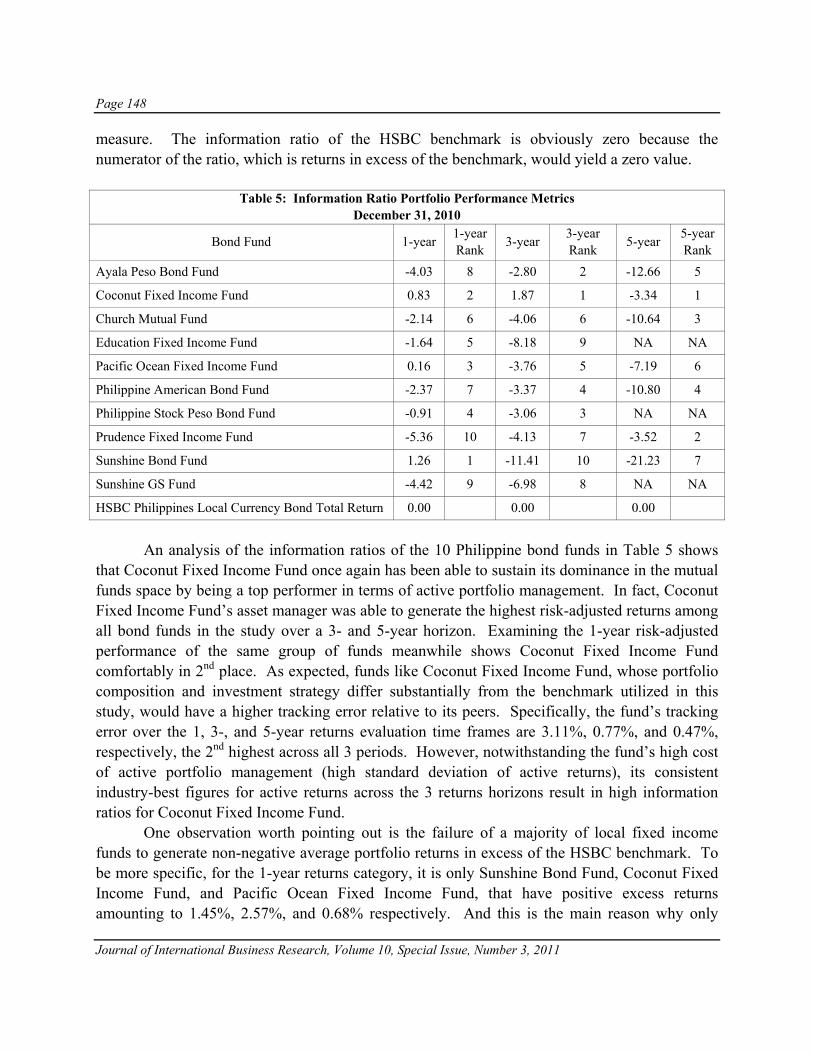
Page 148
Journal of International Business Research, Volume 10, Special Issue, Number 3, 2011
measure. The information ratio of the HSBC benchmark is obviously zero because the numerator of the ratio, which is returns in excess of the benchmark, would yield a zero value.
Table 5: Information Ratio Portfolio Performance Metrics December 31, 2010
Bond Fund 1-year 1-year Rank 3-year 3-year
Rank 5-year 5-year Rank
Ayala Peso Bond Fund -4.03 8 -2.80 2 -12.66 5
Coconut Fixed Income Fund 0.83 2 1.87 1 -3.34 1
Church Mutual Fund -2.14 6 -4.06 6 -10.64 3
Education Fixed Income Fund -1.64 5 -8.18 9 NA NA
Pacific Ocean Fixed Income Fund 0.16 3 -3.76 5 -7.19 6
Philippine American Bond Fund -2.37 7 -3.37 4 -10.80 4
Philippine Stock Peso Bond Fund -0.91 4 -3.06 3 NA NA
Prudence Fixed Income Fund -5.36 10 -4.13 7 -3.52 2
Sunshine Bond Fund 1.26 1 -11.41 10 -21.23 7
Sunshine GS Fund -4.42 9 -6.98 8 NA NA
HSBC Philippines Local Currency Bond Total Return 0.00 0.00 0.00
An analysis of the information ratios of the 10 Philippine bond funds in Table 5 shows
that Coconut Fixed Income Fund once again has been able to sustain its dominance in the mutual funds space by being a top performer in terms of active portfolio management. In fact, Coconut Fixed Income Fund’s asset manager was able to generate the highest risk-adjusted returns among all bond funds in the study over a 3- and 5-year horizon. Examining the 1-year risk-adjusted performance of the same group of funds meanwhile shows Coconut Fixed Income Fund comfortably in 2nd place. As expected, funds like Coconut Fixed Income Fund, whose portfolio composition and investment strategy differ substantially from the benchmark utilized in this study, would have a higher tracking error relative to its peers. Specifically, the fund’s tracking error over the 1, 3-, and 5-year returns evaluation time frames are 3.11%, 0.77%, and 0.47%, respectively, the 2nd highest across all 3 periods. However, notwithstanding the fund’s high cost of active portfolio management (high standard deviation of active returns), its consistent industry-best figures for active returns across the 3 returns horizons result in high information ratios for Coconut Fixed Income Fund.
One observation worth pointing out is the failure of a majority of local fixed income funds to generate non-negative average portfolio returns in excess of the HSBC benchmark. To be more specific, for the 1-year returns category, it is only Sunshine Bond Fund, Coconut Fixed Income Fund, and Pacific Ocean Fixed Income Fund, that have positive excess returns amounting to 1.45%, 2.57%, and 0.68% respectively. And this is the main reason why only

Page 149
Journal of International Business Research, Volume 10, Special Issue, Number 3, 2011
these 3 funds have positive information ratios. For the 3-year returns, only Coconut Fixed Income Fund had a positive active return of 1.44%; hence, the 1.87 information ratio. None of the fixed income funds was able to yield a positive information ratio in the 5-year returns classification. The implication of this is that active management by Philippine fixed income fund managers over the long-term has been ineffective in outperforming a passive index-tracking investment. This somewhat corroborates the belief of some that beating the market using active portfolio-tilting strategies over the long-run is a difficult task. Moreover, the negative information ratios for the 5-year returns also suggest that investors cannot seek to be compensated for idiosyncratic risks that can be diversified away by passively positioning in a diversified market portfolio of bonds over a long period of time.
CONCLUSIONS AND RECOMMENDATIONS
Performance evaluation is a critical step in the portfolio management process, particularly
in determining whether a fund manager has done his job of creating value for his clients more than what is expected. Financial economics has set forth a number of quantitative tools to assess the performance of mutual funds. These analysis techniques look at the historical excess returns of investment portfolios and adjust them for their respective risk qualities to facilitate an apples-to-apples comparison among funds in the investment universe. The four composite measures of portfolio performance that were applied in this study were the Treynor, Sharpe, Jensen, and information ratio risk-adjusted returns metrics. The primary advantage of using these risk-adjusted returns ratios is that they allow analysts and investors to rank mutual funds, and for some of these composite measures, quantify an absolute amount of realized alpha, or abnormal returns. The objective of this research undertaking is to determine whether Philippine fixed income fund managers have been realizing alpha for mutual fund shareholders and to discover which among the local asset management firms have consistently been outperforming or trailing the benchmark or market index.
After having applied all 4 portfolio performance measurement criteria to the returns on Philippine bonds funds over a 1-, 3-, and 5-year evaluation horizon, the proponent was able to identify consistently performing and underperforming mutual funds, both in terms of relative ranking as well as absolute returns performance. Moreover, although the 4 performance appraisal tools provide different approaches to controlling mutual fund returns for uncertainty and for determining relative or absolute outperformance, a number of industry-wide generalizations were arrived at based on the consistent results of the performance metrics. Firstly, after examining the 1-year risk-adjusted returns of fixed income investment companies in the Philippines, it is clear from the numbers that a majority of these funds on average have been able to beat the returns on a passive buy-and-hold T-Bill position. However, after observing the uncertainty-controlled returns of these same mutual funds over the intermediate- and long-term, most local fund managers seem to encounter difficulty on average outperforming the returns on a

Page 150
Journal of International Business Research, Volume 10, Special Issue, Number 3, 2011
hold-to-maturity FXTN investment; hence, negative excess returns. These have led to mostly negative Treynor and Sharpe metrics over the 3- and 5-year periods.
Relative to the returns on the market index used by most Philippine fund managers to benchmark fixed income portfolio performance against, the returns on bond funds pale in comparison whether it be in the short-, medium-, or long-run, as seen in the mostly negative active returns and information ratios of these portfolios. Although there are a few fund managers that were able to provide returns in excess of the benchmark over the 1-, and 3-year time periods, these were merely a handful, indicating a general difficulty by asset management firms to generate alpha by focusing on non-market sources of return. This struggle to produce returns via active portfolio management is even more pronounced when viewed in the long-run, where none of the fund managers was successful in beating the benchmark return on a risk-adjusted basis. This finding is coherent with the notion that it is impossible to beat the market in the long-run.
From an absolute excess returns standpoint, the Jensen’s alpha measure allowed the proponent to determine whether fixed income fund managers in the Philippines were optimizing their skill in predicting market turns and identifying mispriced bonds to beat the market. With the exception of just 3 funds, none of the other investment companies had positive Jensen’s alphas over a 1-year period. And similar to the results of the information ratio analysis, none of the fund managers generated a positive alpha in the long-run, once again validating the perception that it is a daunting task to produce abnormal returns on average over long periods of time.
One of the major shortcomings of the local mutual funds association is its categorization of fixed income funds with different investment styles and portfolio revaluation policies within the same peer group. As observed, funds with significant accrual exposures are compared directly to other funds that have heavy investments in securities designated at fair value. This gives rise to issues in comparability and may render the results of the risk-adjusted performance analysis invalid, especially if these differences are not recognized or highlighted in the appraisal. A workaround to this problem for future studies of similar nature would be to purposively select a sample of funds with similar investment attributes. Although the risk-adjustment process of the composite portfolio performance measures presented in this study are intended to make funds comparable regardless of their differences in risk exposure, performance analysts in the industry have the tendency to compare funds with similar styles.
For future studies, the proponent recommends the use of regression analysis to estimate some of the inputs to the performance metrics, including beta for the Treynor ratio and Jensen’s alpha. Alpha estimation using regression is likewise highly recommended for future researchers to ensure that there is enough statistical basis in claiming that a fund manager has indeed shown skill in generating abnormal returns for his clients. Since Jensen’s alpha was applied in this study as an absolute measure of abnormal returns, future studies may consider risk-adjusting the alpha measure by way of dividing the computed Jensen’s alpha metric with the beta coefficient used, similar to the risk-adjustment procedure under the Treynor performance criterion. Using a

Page 151
Journal of International Business Research, Volume 10, Special Issue, Number 3, 2011
multi-factor model of risk and return such as the APT could also be considered in lieu of the CAPM to proxy for the risk premium in the Jensen’s alpha methodology.
As for the risk-free rate, the fixing yield on Philippine government securities was used in this research as the representation for the riskless asset return. Future researchers on fund performance assessment may want to consider using the reference rate on done transactions in the secondary government securities market in lieu of the fixing rate. It is noteworthy that both fixing yields and reference yields on government securities are stated gross of applicable withholding taxes in the Philippines. Since the NAVPS of mutual funds from which the rolling returns are derived are reported net of all relevant administrative costs and management fees, future studies could consider restating the fixing or reference yields net of the withholding tax.
Benchmark selection is likewise a major issue in the asset management industry, particularly on the aspect of performance assessment. As discussed previously, drawing conclusions about an asset manager’s ability to generate abnormal returns may be misleading if an appropriate benchmark is not used. Purposive sampling or the use of a fund-specific benchmark may address the benchmark selection problem though this comes at the price of not being able to truly determine absolute returns outperformance relative to an index. The proponent suggests that for relative ranking performance appraisal criteria such as the Treynor and information ratios, a fund-specific benchmark be used, whereas for the Jensen’s alpha metric, a single index must be utilized.
Sample-wise, future research initiatives focusing on investment fund performance appraisal in the Philippines could be applied to other sub-sectors within the local mutual fund industry. This study concentrated on risk-adjusted returns evaluation for Philippine Peso-denominated bond funds that are members of the local mutual funds association. Money market mutual funds, Dollar-denominated bond funds, and global bond funds can also be assessed using the methodology presented in this research paper. The composite portfolio performance measures could likewise be applied to Philippine fixed income UITFs. An interesting research endeavor would be to implement a comparison of the risk-adjusted returns performance of Philippine fixed income mutual funds versus UITFs as competing asset classes.
REFERENCES
Brown, K.C. & F.K. Reilly (2009). Analysis of Investments and Management of Portfolios (Ninth Edition).
Canada: South-Western Cengage Learning. Bodie, Z., A. Kane, & A.J. Marcus (2009). Investments (Eighth Edition). New York, NY: McGraw-Hill/Irwin. Chua, E.G., J.G. Geocaniga, N. Pena, A.G. Yambao (2008). Evaluating Data Envelopment Analysis as an
Alternative Fund Performance Appraisal Tool to Traditional Composite Measures of Portfolio Performance: A Philippine Mutual Fund Industry Risk-Return Analysis for the Years 2003-2007. Unpublished undergraduate thesis, De La Salle University-Manila.
Cocolife Asset Management Company, Inc. Retrieved January 1, 2011, from http://www.cocolifeasset.i.ph Elton, E.J., M.J. Gruber, S.J. Brown, & W.N. Goetzmann (2011). Modern Portfolio Theory and Investment
Analysis (Eighth Edition). Hoboken, NJ: John Wiley & Sons (Asia) Pte Ltd.

Page 152
Journal of International Business Research, Volume 10, Special Issue, Number 3, 2011
Investment Company Association of the Philippines. Retrieved January 1, 2011, from http://www.icap.com.ph Unit Investment Trust Fund Online. Retrieved January 1, 2011, from http://www.uitf.com.ph Valderrama, H.S. (2003). Philippine Mutual Funds and Common Trust Funds: How Different Are They? Retrieved
January 1, 2011 from http://www.upd.edu.ph/~cba/docs/hsv_ctf_study.pdf Valderrama H.S. & C.C. Bautista (2003). The Development and Performance of the Philippine Mutual Funds
Industry. Retrieved January 1, 2011 from http://www.upd.edu.ph/~cba/research.htm

Page 153
Journal of International Business Research, Volume 10, Special Issue, Number 3, 2011
BUSINESS ETHICS IN JAPAN : TAKING A CLOSER LOOK AT THE ROLE OF AGE
Jeanne H. Yamamura, University of Nevada Reno
Yvonne Stedham, University of Nevada Reno
ABSTRACT
This study focused on the relationship between age and business ethics in Japan. We examined ethical judgments made by Japanese men and women in business situations using justice, utilitarian, and egoism criteria while controlling for gender and gender-age interaction effects. Since individuals’ ethical judgment depends on the stage of their moral development and the stage of moral development is related to age, we expected that relationships between the ethical perspectives and age existed. Our results support such relationships.
INTRODUCTION
The global population is aging rapidly, faster than at any time in the past. By 2050, in developed countries, those over 60 are expected to outnumber people under 15 by a ratio of two to one (Fishman, 2010). This changing age mix in the world’s population is expected to profoundly impact how business is conducted everywhere.
Japan leads the way in the “graying” of the world. Japan’s total population in 2009 was 127.51 million, a decrease of 180,000 from 2008 and a continuation of the decline since its peak in 2004. Current projections reduce Japan’s shrinking population to 95 million by 2050. In 2009, citizens aged 65 years and over comprised 22.7% of the total population. By 2050, the percentage is estimated to reach 39.6% (Statistics Bureau Japan, 2010).
Generally, negative prognoses have accompanied this news ranging from the harmful effects of the Japanese “gray menace” on innovation, investment, international security, and business cycle volatility to the possible extinction of advanced, post-industrial societies (e.g. Bainbridge, 2009; Glosserman & Tsunoda, 2009; Inoguchi, 2009; Jaimovich & Siu, 2009). But is the aging of Japan’s population only bad news?
From an ethical point of view, age has long been considered a key factor in moral judgment. Supported by Kohlberg’s (1984) six-stage theory of moral reasoning, individuals progress through developmental stages over the course of their lifetimes, achieving the most advanced levels with age. In general, it has been found that ethical behavior increases with age (e.g., Borkowski & Ugras, 1998; Conroy et al., 2009; Peterson et al., 2001). Although much of this research has been conducted with North American samples, similar results have been obtained for other countries (e.g., Chan et al., 2002; Sudani et al., 2009; Wimalasiri, 2001).

Page 154
Journal of International Business Research, Volume 10, Special Issue, Number 3, 2011
However, while exploring the relationship between age and ethical judgment, these studies provide rather limited insights into the underlying rationale for such a relationship. This study focuses on the relationship between age and ethical judgment in business situations in Japan and in contrast to existing studies, several ethical perspectives (justice, egoism, and utilitarianism) will be employed to explore the relationship between age and ethical judgment. We relate the ethical perspectives to Kohlberg’s model of moral development which allows us to offer conceptual ideas for the existence of a relationship between age and ethical judgment.
BACKGROUND Age and Ethical Judgment Age has long been recognized as a critical factor in the ethics literature with research results generally supporting its inclusion. Overall, the results imply that older individuals are more ethical. Several studies show that increased age is linked to more conservative and strict ethical judgments and more inflexible opinions about what constitutes ethical behavior (e.g., Arlow, 1991; Barnett & Karson, 1989). A meta-analysis of 35 studies that included age as a factor concluded that ethicality seemed to increase as people mature (Borkowski & Ugras, 1998). Peterson et al. (2001) found younger business professionals to display a lower ethical standard and to be more influenced by external factors in making ethical judgments. Similarly and more recently, Conroy et al. (2009) found older business professionals to be less likely to judge ethically questionable behavior as acceptable.
In research involving non-North American participants, age has also been linked to increased ethicality. For example, Chan et al. (2002) reported younger Chinese executives as more likely to engage in unethical activities than older executives. Wimalasiri (2001) determined that increasing age among Australian participants resulted in stronger moral reasoning ability and Sidani et al. (2009) concluded that age provided a better explanation of ethical sensitivity among Lebanese workers than gender. Volkema (2004) found ethical standards increasing with age in a nine-country study. Studies that focused on Japan found younger consumers to be less ethical than older consumers, that opposition to tax evasion increased with age, and that while older respondents were more ethical than younger respondents, the moral judgments of men and women converged with age (Aldrich & Kage, 2003; Erffmeyer et al., 1999; McGee, 2007). Stages of Moral Development: Kohlberg’s Model
Although empirical work clearly supports the role of age in ethical judgment, few studies address the underlying rationale for the relationship. Why and how are age linked to ethical

Page 155
Journal of International Business Research, Volume 10, Special Issue, Number 3, 2011
judgment? It has been suggested that the “missing” link may be found in understanding how individuals learn to make moral judgments. For instance, Ferrell et al. (2002, p. 106) point out that “cognitive moral processing is a crucial element in ethical decision-making.”
A well recognized and accepted model of moral development was presented by Kohlberg (1969, 1984). Based on this model, moral reasoning advances through six stages, with increasing ability to address moral dilemmas at each stage. Accordingly, people make different decisions in similar ethical situations because they are at different stages of cognitive moral development. Table 1 provides a summary of the stages in Kohlberg’s model.
The first two stages (pre-conventional phase) suggest that an individual addresses a moral dilemma considering primarily consequences of alternative actions for him- or herself (How can I avoid punishment? and What's in it for me?). The needs of others may occasionally be considered but generally in a pragmatic way (You scratch my back and I’ll scratch yours). During the conventional phase (stages 3 and 4), individuals’ decisions are still motivated by personal consequences but now consider the well-being of others as equally important.
Table 1: Kohlberg’s Stages Of Moral Development (Kohlberg 1971)
Stage Level Description of factors that determine “rightness” of an action
1 Pre-conventional
Physical consequences, e.g., punishment
2 Personal gain and satisfaction of own needs
3 Conventional
What pleases or helps others
4 Authority and need to maintain social order
5 Post-conventional
Laws or institutionalized rules of society
6 Conscience and universal ethical principles such as justice and equality
This is the stage where strong support for the social order begins to influence individuals’
cognitions. What is considered right depends on the individual’s perception of his or her duty to society rather than specific people. At the final, post-conventional phase (stages 5 and 6), individuals are guided by increasingly abstract principles rather than by obedience and avoidance of negative consequences or perceptions of duty to others or society as in the previous two phases. In the post-conventional phase, the individual moves to identify and support the general individual rights and standards that have been agreed upon by society as a whole. This leads to determination of universal ethical principles, such as justice and equality, and the belief that they should be followed by all.
An individual progresses through the stages over the course of a lifetime; thus, age is positively associated with the level of moral development. With increased age and life experience, individuals become more aware of the negative consequences of unethical actions (Miesling & Preble, 1985; Wood et al., 1988) and have increased knowledge, understanding, and
Page 156
Journal of International Business Research, Volume 10, Special Issue, Number 3, 2011
appreciation of what is considered “right” and “wrong” in their culture through longer ongoing exposure to tradition and custom (Mudrack, 1989).
Kohlberg (1971) proposed that his model was universally applicable, independent of cultural or societal circumstances. This claim and the model itself have received considerable criticism over the years (e.g., Snarey, 1985; Simpson, 1994). Such criticism has included an exclusively Western orientation, gender bias due to the use of data from young males only, and the assumption that there is only one form of ethical maturity, stage 6 reasoning. Despite the controversy, the six stages in the model have become generally accepted as representative of how human beings develop with respect to making ethical assessments and are widely used in ethical value research (e.g., Henry, 2001). In addition, recent studies indicate that the Kohlberg model can be successfully applied to Japanese professionals (e.g., Davison et al., 2009). Ethical Perspectives and Moral Development: The Missing Link?
Since ancient historical times, much attention has been focused on understanding “ethics” and on how human beings make or should make ethical judgments. While ethical principles and judgments may be approached utilizing several normative theories, three are of particular interest in an examination of the relationship between age, moral development, and ethical decision making: egoism, utilitarianism, and justice.
Egoism and utilitarianism are consequentialist theories that incorporate values related to an individually-based versus a community-based focus. Egoism looks primarily at the individual and his/her self-interest (Shaw, 1999). Here, a decision is seen as ethical if it benefits the decision-maker. The criteria used to evaluate an ethical dilemma are to what extent an action is self promoting/not self promoting, self sacrificing/not self sacrificing, and personally satisfying/not personally satisfying.
In the development of moral understanding, Kohlberg’s early stages of moral development suggest that the criteria for moral judgments at this point center around the benefits for the individual derived from certain actions while lacking a consideration of consequences of the decision for others. Therefore, we propose that the egoism perspective for ethical judgment captures the pre-conventional aspects of moral development (stages 1 and 2).
In contrast, the primary focus of utilitarianism is a consideration of possible consequences of alternative actions for all parties. Specifically, when judging an ethical dilemma considering utilitarian principles, the decision-maker determines to what extent the decision produces the greatest utility for most people, maximizes benefits while minimizing harm, and leads to the greatest good for the greatest number of people. Hence, based on utilitarian principles, an action is considered ethical if it is seen as creating benefits for most people important to the decision-maker. The utilitarianism perspective seems to be related to stages 3 and 4, the conventional phase of Kohlberg’s model, where an individual’s moral judgment begins to be influenced by social awareness.
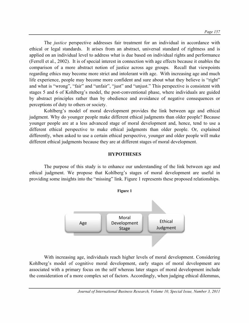
Page 157
Journal of International Business Research, Volume 10, Special Issue, Number 3, 2011
The justice perspective addresses fair treatment for an individual in accordance with ethical or legal standards. It arises from an abstract, universal standard of rightness and is applied on an individual level to address what is due based on individual rights and performance (Ferrell et al., 2002). It is of special interest in connection with age effects because it enables the comparison of a more abstract notion of justice across age groups. Recall that viewpoints regarding ethics may become more strict and intolerant with age. With increasing age and much life experience, people may become more confident and sure about what they believe is “right” and what is “wrong”, “fair” and “unfair”, “just” and “unjust.” This perspective is consistent with stages 5 and 6 of Kohlberg’s model, the post-conventional phase, where individuals are guided by abstract principles rather than by obedience and avoidance of negative consequences or perceptions of duty to others or society.
Kohlberg’s model of moral development provides the link between age and ethical judgment. Why do younger people make different ethical judgments than older people? Because younger people are at a less advanced stage of moral development and, hence, tend to use a different ethical perspective to make ethical judgments than older people. Or, explained differently, when asked to use a certain ethical perspective, younger and older people will make different ethical judgments because they are at different stages of moral development.
HYPOTHESES The purpose of this study is to enhance our understanding of the link between age and ethical judgment. We propose that Kohlberg’s stages of moral development are useful in providing some insights into the “missing” link. Figure 1 represents these proposed relationships.
Figure 1
With increasing age, individuals reach higher levels of moral development. Considering Kohlberg’s model of cognitive moral development, early stages of moral development are associated with a primary focus on the self whereas later stages of moral development include the consideration of a more complex set of factors. Accordingly, when judging ethical dilemmas,
AgeMoral
Development Stage
EthicalJudgment

Page 158
Journal of International Business Research, Volume 10, Special Issue, Number 3, 2011
younger people are expected to be more concerned with the consequences of a decision for themselves and to less concerned with the consequences for the larger community than older people. In addition, younger people are expected to be less aware of and thus less certain when applying abstract ethical principles such as justice than older people.
In summary, previous research on business ethics, age, and moral development implies:
• A positive relationship between ethics and age • This relationship has been shown to exist across different countries including
Japan • Kohlberg’s model of cognitive moral development provides theoretical support
for the relationship between age and ethics • Individuals who are younger are likely to be in the pre-conventional and
conventional phases of Kohlberg’s model of cognitive moral development. Utilitarian and egoism perspectives of ethics are related to age through these two phases.
• Individuals who are older are more aware of and more certain regarding ethical standards and norms. Therefore, age is related to ethical judgment through the justice perspective of ethics.
In addition, previous research on business ethics found gender-based differences (e.g.,
Albaum & Peterson, 2006; Dawson, 1997; Glover et al., 2002; Loo 2003; Peterson et al., 2001; Roxas & Stoneback, 2004; Stedham et al., 2006) as well as situational effects on ethics judgment (e.g., Beekun et al., 2003a, 2003b; Cohen et al., 1996; Reidenbach & Robin, 1988). As a result, both gender and situation must be included in our model relating ethical judgment to age.
Considering the theoretical relationships of age, moral development, and ethical perspectives as well as the results of previous studies on ethical judgment, we propose the following model:
Ethical Judgment = f (Age, Gender, Age X Gender, Situation)
Overall, we expect that age differences will be reflected in differences in ethical
judgment based on egoism, utilitarian, and justice criteria because age is related to moral development and the stages of moral development are related to the ethical perspectives. The egoism criteria present self-promotion and personal satisfaction as ethically appropriate objectives. This focus on the consequences (benefits) to the decision maker of a particular ethical decision exemplifies the pre-conventional phase of Kohlberg’s model of moral development which is reflected differently across age groups. Hypothesis 1 is thus:
Page 159
Journal of International Business Research, Volume 10, Special Issue, Number 3, 2011
H1: When employing egoism criteria to judge the ethical content of an action, the judgments will differ by age group.
In contrast, the utilitarian criteria focus on benefits to others, specifically, greatest utility
and maximization of benefits to the largest number are important to the decision maker, as the requirements for ethical behavior. This emphasis on communal concerns reflects the concern for pleasing others and maintenance of the social order of the conventional phase of Kohlberg’s model. Judgments employing utilitarian criteria are expected to differ across age groups. We propose that:
H2: When employing utilitarian criteria to judge the ethical content of an
action, the judgments will differ by age group. The justice criteria provide a more abstract black and white framing for ethical judgment
– fair/unfair, just/unjust. They enable capture of individual perceptions of right and wrong. Individuals in the post-conventional phase of Kohlberg’s model have moved beyond self and others to more abstract ideas of moral values and principles. The justice criteria reflect the post-conventional phase development of universal ethical principles and are expected to be utilized in judgments differently across age groups. Hence, hypothesis 3 is:
H3: When employing justice criteria to judge the ethical content of an action,
the judgments will differ by age group.
METHODOLOGY Sample
The convenience sample consisted of 100 Japanese business students completing post-graduate studies in accounting in Japan. The data were collected during late 2004 and early 2005. It should be noted that in 2005 major changes occurred in accounting education as a result of the 2003 amendments to the Certified Public Accountant (CPA) law in Japan. Beginning in 2005, new graduate schools of accountancy were created in the university system enabling students to complete graduate programs while preparing for the CPA exam. Previously, those seeking to take the CPA exam enrolled in private professional schools. This sample was drawn from students enrolled in a private school.
Graduate-level business students are frequently utilized as a proxy for business people in a wide range of business studies. This usage is based on research indicating a high degree of similarity between the two groups (e.g., Dubinsky & Rudelius, 1980; Harris & Sutton, 1995). In ethics studies, in particular, students recognized ethical issues and made decisions in a manner

Page 160
Journal of International Business Research, Volume 10, Special Issue, Number 3, 2011
similar to that of corporate managers (Lysonski & Gaidis, 1991). However, the findings of other researchers imply that students may be less ethical than business professionals (e.g., Dupont & Craig, 1996). As a result, caution will be exercised in interpreting the results.
Table 2: Sample
Category
AGE
20 to 29 12
30 to 39 67
40 and over 21
Total 100
GENDER
Male 72
Female 28
Total 100
While the average student was in his/her 30’s, the sample included a relatively wide age dispersion ranging from early 20’s to over 50. Approximately two-thirds of the sample was male while one-third was female. Table 2 provides summary information regarding the sample. Measures
Participants assessed actions taken in three business-related scenarios which provided the contextual stimulus for the evaluation process (Alexander & Becker, 1978). We utilized Reidenbach and Robin’s (1988, 1990) pre-validated scenarios and sets of ethical criteria which have demonstrated high reliability and construct validity in numerous research settings (see Tables 3 and 4). Responses made utilized a 7-point Likert scale and generally indicate 1 = ethical while 7 = unethical.
Cronbach alpha scores for the measures were examined to verify instrument reliability. Inter-item coefficient alphas were calculated for the egoism, utilitarian, and justice judgment variables for Japan for each of the three scenarios, yielding nine in total. The alpha reliabilities ranged from .89 to .70, indicating internal consistency (Nunnally, 1967). The sole exception (out of 9) was the egoism variable for the sales scenario that received a Cronbach alpha score of .36. The questionnaire was completed in Japanese. The translated questionnaire was back-translated with appropriate revisions made to ensure functional equivalence.

Page 161
Journal of International Business Research, Volume 10, Special Issue, Number 3, 2011
Table 3: Ethics Instrument Scales
Ethical Perspective
Items (Seven-point Likert scale – 1 to 7)*
Egoism
Self promoting/not self promoting
Self sacrificing/not self sacrificing
Personally satisfying/not personally satisfying
Utilitarianism
Produces greatest utility/produces the least utility
Maximizes benefits while minimizes harm/minimizes benefits while maximizes harm
Leads to the greatest good for the greatest number/leads to the least good for the greatest number
Justice Just/unjust
Fair/unfair
*Generally speaking, in the above bipolar scales, 1 = self-satisfying or maximizes benefits (ethical) whereas 7 = not self-satisfying or satisfies smallest number (unethical).
Table 4: Scenarios
Scenario 1: Retail – Automobile. A person bought a new car from a franchised automobile dealership in the local area. Eight months after the car was purchased, he began having problems with the transmission. He took the car back to the dealer, and some minor adjustments were made. During the next few months he continually had a similar problem with the transmission slipping. Each time the dealer made only minor adjustments on the car. Again during the thirteenth month after the car had been bought the man returned to the dealer because the transmission still was not functioning properly. At this time, the transmission was completely overhauled. Action: Since the warranty was for only one year (12 months from the date of the purchase), the dealer charged the full price for parts and labor.
Scenario 2: Neighborhood Store. A retail grocery chain operates several stores throughout the local area including one in the city’s ghetto area. Independent studies have shown that the prices do tend to be higher and there is less of a selection of products in this particular store than in the other locations. Action: On the day welfare checks are received in the area of the city the retailer increases prices on all of his merchandise.
Scenario 3: Salesman. A young man, recently hired as a salesman for a local retail store, has been working very hard to favorably impress his boss with his selling ability. At times, this young man, anxious for an order, has been a little over-eager. To get the order, he exaggerates the value of the item or withholds relevant information concerning the product he is trying to sell. No fraud or deceit is intended by his actions, he is simply over-eager. Action: His boss, the owner of the retail store, is aware of the salesman’s actions but has done nothing to stop such practice.
Statistical Methods
An initial assessment of the relationships among the variables is provided through consideration of the descriptive statistics and by correlation analysis. Assessment of the overall model was made using a repeated measures MANCOVA. The multivariate F-test was more

Page 162
Journal of International Business Research, Volume 10, Special Issue, Number 3, 2011
appropriate given the repeated judgments made by the subjects in the three situations and the resultant high correlation among the dependent variables, Egoism, Utilitarianism, and Justice (see Table 6). Univariate F-tests (ANCOVAs) were used to provide an individual assessment of hypothesized age differences for each of the three ethical perspectives. Finally, for informational and discussion purposes, the ethical judgments by age and ethical perspective appear in Table 8.
RESULTS
Table 5: Descriptive Statistics
Variable N Mean Std. Dev. Range
Judgment using egoism criteria
Overall 83 5.40 .82 3.44 to 7
Age – 20’s 11 4.89 .76 3.56 to 5.89
Age – 30’s 55 5.37 .85 3.44 to 7
Age – 40+ 17 5.83 .51 4.56 to 6.44
Judgment using utilitarian criteria
Overall 85 5.12 .92 3 to 7
Age – 20’s 12 4.44 .90 3 to 6
Age – 30’s 56 5.13 .85 3.22 to 6.89
Age – 40+ 17 5.54 .92 3.89 to 7
Judgment using justice criteria
Overall 86 5.62 .89 3.33 to 7
Age – 20’s 12 5.04 .96 3.33 to 6.17
Age – 30’s 57 5.59 .90 3.83 to 7
Age – 40+ 17 6.10 .49 5 to 6.67
Note: The number of responses exceeded sample size as responses were received from each subject for each of 3 different scenarios.
Descriptive statistics and correlations for the study variables are presented in Tables 5
and 6. The mean scores increase with age for all ethical criteria providing initial support for Hypotheses 1, 2, and 3. Correlation analysis reveals relatively high and significant correlations among the different ethical perspective variables.
In the multivariate tests, age was significant for all three ethical perspectives (egoism - F2,74 = 5.876, p < .000; justice - F2,74 = 13.410, p < .003; utilitarianism - F2,74 = 13.391, p < .005). Situation was also significant (F6,292 = 10.353, p < .000) indicating the presence of significantly

Page 163
Journal of International Business Research, Volume 10, Special Issue, Number 3, 2011
different responses by scenario. Interestingly, gender and age X gender were not significant. The univariate ANCOVAs shown in Table 7 revealed significant age effects for each of the three ethical judgments providing support for Hypotheses 1, 2, and 3.
Table 6: Correlations
Variables 1 2
1. Judgment employing egoism criteria
2. Judgment employing utilitarian criteria .616**
3. Judgment employing justice criteria .843** .621**
* = p < .05; ** = p < .01
Table 7: Univariate Ancova For Ethical JudgmentsSource DF Sum of Squares Mean Square F value P value
Judgment Using Egoism Criteria Overall model 7 180.571 25.796 19.688 .000 Error 254 332.803 1.310
Corrected total 261 513.374 Age 2 20.140 10.070 7.685 .001 Gender 1 .817 .817 .624 .430 Age * Gender 2 3.720 1.860 1.420 .244 Situation 2 159.810 79.905 60.985 .000 Judgment Using Utilitarian Criteria Overall model 7 55.912 7.987 5.357 .000 Error 256 381.718 1.491 Corrected total 263 437.63 Age 2 27.020 13.510 9.060 .000 Gender 1 .431 .431 .289 .591 Age * Gender 2 1.513 .757 .507 .603 Situation 2 26.553 13.277 8.904 .000 Judgment Using Justice Criteria Overall model 7 61.236 8.748 5.115 .000 Error 263 449.825 1.710 Corrected total 270 511.061 Age 2 26.450 13.225 7.732 .001 Gender 1 .024 .024 .014 .906 Age * Gender 2 1.762 .881 .515 .598 Situation 2 32.466 16.233 9.491 .000
Table 8 provides a summary of the ethical judgments by situation, age, and ethical
perspective clearly demonstrating the changes in ethical judgment with increasing age.

Page 164
Journal of International Business Research, Volume 10, Special Issue, Number 3, 2011
Table 8: Ethical Judgments By Scenario, Age, And Ethical Perspective
Ethical Perspective
Age
20 to 29
30 to 39
40 and up Difference: Oldest -
Youngest Age Group AUTO Egoism 5.36 6.05 6.23 0.87 Utilitarianism 5.22 5.29 5.78 0.56 Justice 5.25 5.70 6.45 1.20 GROCERY STORE Egoism 5.42 5.88 6.51 1.09 Utilitarianism 4.30 5.30 5.82 1.52 Justice 5.62 5.86 6.38 0.76 SALESPERSON Egoism 4.03 4.25 4.70 0.67 Utilitarianism 3.78 4.71 5.07 1.29 Justice 4.25 5,21 5.50 1.25 ALL SCENARIOS Egoism 4.94 5.39 5.81 0.87 Utilitarianism 4.43 5.10 5.56 1.13 Justice 5.04 5.59 6.11 1.07 Responses made utilized a 7-point Likert scale and generally indicate 1 = ethical while 7 = unethical.
DISCUSSION AND CONCLUSIONS
This study investigated the relationship between age and business ethics in Japan. We
examined age and its relationship to ethical judgments made by Japanese business people using egoism, utilitarian, and justice criteria while controlling for potential gender and situation effects. We suggested that relationships between these ethical perspectives and age existed because individuals’ ethical judgment depends on their stage of moral development. As hypothesized, we found a significant relationship between age and ethical judgment. For all three ethical perspectives, older respondents found the scenarios to be more unethical than younger respondents. These findings are consistent with Kohlberg’s typology suggesting that older individuals are at more advanced stages of moral development than younger individuals.
Across all scenarios, a comparison of the difference in means between the oldest and youngest respondents for the justice criteria and the egoism criteria revealed a considerably larger difference for the justice criteria (1.07) than for the egoism criteria (.87). This made sense since the justice perspective was the most “abstract” ethical view included in this study and represented the most advanced level of ethical development (the post-conventional phase). Considering the results of previous research indicating that older people are more set in their views of right and wrong than younger people, our results highlighted that the ability to apply abstract moral rules “comes with age.”

Page 165
Journal of International Business Research, Volume 10, Special Issue, Number 3, 2011
When using egoism criteria, the mean of 4.94 for the youngest age group compared to a mean of 5.81 for the oldest age group reflected clear differences but not as strongly as apparent with the justice criteria. Younger respondents were more accepting of the described action when considering the consequences of the action for the decision-maker only than the older respondents. In turn, older respondents did not feel that the action was justified simply because it benefited the decision maker. This was clearly consistent with the idea that the younger respondents are likely to be at the earlier stages of moral development. Differences in ethical judgment across age groups appeared also by situation. The scenarios evidenced situations with differing degrees of “moral intensity.” The grocery store scenario was judged “most heinous” by the participants while the salesman scenario was considered the least offensive.
Interestingly, the largest difference in judgment of the oldest versus the youngest respondents in the grocery store scenario appeared for the utilitarian criteria (a difference of 1.52 in the two group’s means). This was the largest difference observed for all the scenarios and ethical perspectives. Conjecturing, we might propose that this result may not only reflect the difference in stages of moral development but also differences in values as to the importance of “community” or collectivism between the younger and older generations of Japanese. A similar result was found for the salesman scenario – for utilitarian criteria, the difference in the means for the oldest and the youngest respondents was 1.29 (the second largest across all scenarios and ethical criteria). Note that overall, across all scenarios, we found the largest difference between youngest and oldest respondents for the utilitarian perspective (1.13) further supporting the idea of differences in values related to collectivism.
In the auto scenario, the differences in judgment between youngest and oldest were not as large as in the other scenarios except for the justice perspective (a difference between the means for youngest and oldest of 1.20). In this scenario, more abstract “what is right, what is wrong” considerations played a role – considerations more difficult for younger respondents than older ones because of the difference in moral development. The differences between the youngest and oldest groups were not as apparent for the egoism and utilitarian criteria as the benefits to self were possibly overridden by the perceived blatant “injustice” of the situation and because the potential benefits of the actor’s decision for others were limited.
The differing ethical perspectives utilized by participants across the scenarios may be indicative of “stage volatility” as noted by Snell (1996) and Davison et al. (2009). Stage volatility is evidenced by the simultaneous consideration of factors pertaining to different stages of ethical reasoning. Snell et al. (1997) noted “Moral experience becomes increasingly complex and multifaceted, and potentially more volatile, as ethical reasoning capacity increases. Managers who have attained stage six capacity may still experience and be governed by stage one fears and amoral urges and impulses.” The failure to adopt a single primary mode of ethical reasoning, i.e., one ethical perspective, may simply reflect lingering early stage concerns despite the attainment of higher level ethical reasoning capabilities.

Page 166
Journal of International Business Research, Volume 10, Special Issue, Number 3, 2011
An additional finding was that some of the most strict and least strict judgments of ethical behavior from all three age groups appeared using the egoism criteria. Recall that the measure for ethical judgment based on an egoism perspective includes criteria such as self-promoting, personally-satisfying, etc. Perhaps the individualistic aspects of this perspective and its emphasis on self and self-interest resonate more strongly with Japanese participants. Recent literature supports the growth of individualism in Japan (e.g., Kambayashi & Scarborough, 2001; Matsumoto, 2002; Matsumoto et al., 1996), a phenomenon causing some consternation among its formerly more collectivist inhabitants (Hofstede, 2001). The younger age groups have grown up in an era of relative wealth and prosperity, a time in which individualism has grown and concern for the group has lessened. As a result, different ages may respond to “personally-satisfying” and “leads to the greatest good for the greatest number” very differently.
Our results did not reveal a gender difference in ethical judgment. This result was surprising given Japan’s reputation as “one of the most gender-stratified societies” in the world (Verba et al., 1978). While surprising, this result corroborates the lack of gender findings that appeared in Davison et al.’s (2009) study of Japanese information technology professionals. The lack of a difference in ethical judgment by gender may be due to the strong similarities among the women and men in both samples. The movement of women into professional positions in Japan is relatively new and has been slow. Japanese women traditionally have been responsible for the home and the family. As a result, their careers have tended to be low level positions cut off when marriage occurs or children appear. The women in these two studies were women who have chosen advanced business education leading to professional positions or have already progressed to professional positions in a specialized area. Both decisions imply similarity in values and aspirations that may supersede any gender-based differences.
We also did not find a significant age x gender interaction. According to the ANCOVA results, neither younger men and women nor older men and women significantly differed in their judgments of the actions taken. These results differed from those found previously in which gender judgments were found to converge with age (e.g., Aldrich & Kage, 2003). Again, the likely similarities in values among the men and women in the sample may have contributed to this result.
LIMITATIONS AND IMPLICATIONS FOR FUTURE RESEARCH
The results of this study have to be interpreted considering the following caveats. First, the respondents were graduate-level business students completing studies in accounting. This specialized group may not be representative of the population as a whole, limiting our ability to generalize the results of our study. They are, however, a group that will be making business decisions in the future and thus are appropriate for this study. Second, the age variability of the sample was somewhat limited making comparisons by age group more speculative. Caution has been exercised in interpreting the results. Third, it would be desirable to have larger samples for

Page 167
Journal of International Business Research, Volume 10, Special Issue, Number 3, 2011
each of the age groups to allow for additional statistical analyses. Finally, the ethical judgment measure was developed in the U.S. and may be somewhat culture bound. Kohlberg believed his model to be cross-culturally applicable in terms of the different reasoning methods employed, not necessarily the specific ethical beliefs. Prior research and this study provide support for the applicability of the Kohlberg model to Japanese business people.
These caveats notwithstanding, the results of this study have important implications. Clearly, from a theoretical perspective, models and research on ethical judgment need to include age. Age is related to ethical judgment, independent of the ethical criteria used. It appears that Kohlberg’s model of cognitive moral development provides a useful theoretical foundation for the age-ethics relationship and appears to be applicable across cultures. In addition, the largest gap between the age groups appears for utilitarian criteria and not justice criteria. This result needs to be further explored!
Individuals in this study appeared to exhibit “stage volatility” or the simultaneous use of multiple ethical perspectives. Snell et al. (1997) presented such use as persistent lower level fears that continue despite attainment of higher level ethical reasoning capability. It is also possible that such use may simply be individuals choosing (consciously or unconsciously) to employ multiple perspectives in making an ethical decision, i.e., a multidimensional judgment process. Future research exploring this issue to determine whether attainment of pure stage six reasoning is possible (further supporting Kohlberg’s model) or whether ethical reasoning is a multidimensional process (requiring further consideration of Kohlberg’s stages and stage progression).
Practical implications relate to understanding that in business transactions with Japanese businessmen, ethical judgments will differ by age. Older businessmen and women will be stricter in their ethical assessments than their younger counterparts. This may cause challenges in Japanese companies as decision-making is group and consensus based. Differences in values and ethics between younger and older employees may make it more difficult to reach a common decision.
REFERENCES Albaum, G. and Peterson, R.A. (2006). Ethical attitudes of future business leaders: do they vary by gender and
religiosity? Business and Society, 45(3), 300-21. Aldrich, D. and Kage, R. (2003). Mars and Venus at Twilight: A Critical Investigation of Moralism, Age Effects,
and Sex Differences. Political Psychology, 24(1), 23-40. Alexander, C. and Becker, M. (1978). The use of vignettes in survey research. Public Opinion Quarterly, 42:1, 93–
104. Arlow, P. (1991). Personal Characteristics in College Students’ Evaluations of Business Ethics and Corporate
Social Responsibility. Journal of Business Ethics, 10, 63-69. Bainbridge, William S. (2009). Demographic collapse. Futures doi:10.1016/j.fugures.2009.07.005. Retrieved
online 9/5/09.

Page 168
Journal of International Business Research, Volume 10, Special Issue, Number 3, 2011
Barnett, J.H. and Karson, M.J. (1989). Managers, Values and Executive Decisions: An Exploration of the Role of Gender, Career Stage, Organizational Level, Function, and the Importance of Ethics, Relationships, and Results in Managerial Decision-Making. Journal of Business Ethics, 8(10), 747-71.
Beekun, R.I, Stedham, Y., Yamamura, J, and Barghouti, J.A. (2003a). Comparing Business Ethics in Russia and the U.S. International Journal of Human Resource Management, 14, 8 (December), 1333-1349.
Beekun, R., Stedham, Y., and Yamamura, J. (2003b). Business Ethics in Brazil and the U.S.: Egoism and Utilitarianism. Journal of Business Ethics 42, 3, 267-279.
Borkowski, S.C. and Ugras, Y. (1998). Business students and ethics: a meta-analysis. Journal of Business Ethics 17(11), 1117-27.
Chan, R.Y.K., Cheng. L.T.W., and Szeto, R.W.F. (2002). The dynamics of guanxi and ethics for Chinese executives. Journal of Business Ethics 41(4), 327-36.
Cohen, J.R., Pant, L.W., and Sharp, D.J. (1996). A methodological note on cross-cultural accounting ethics research. International Journal of Accounting 31: 55-66.
Conroy, S.J., Emerson, T.L.N., and Pons, F. (2009). Ethical Attitudes of Accounting Practitioners: Are Rank and Ethical Attitudes Related? Journal of Business Ethics DOI 10.1007/s10551-009-0076-2.
Davison, R.M., Martinsons, M.G., Ou, C.X.J., Murata, K., Drummond, D., Li, Y., and Lo, H.W.H. (2009). The Ethics of IT Professionals in Japan and China. Journal of the Association for Information Systems 10(11), 834-859.
Dawson, L.M. (1997). Ethical Differences between Men and Women in the Sales Profession. Journal of Business Ethics 16, 1143-1152.
Dubinsky, A.J. and Rudelius, W. (1980). Ethical beliefs: how students compare with industrial salespeople, in Proceedings of the American Marketing Association Educators Conference, Chicago, pp. 73-76 (Chicago: American Marketing Association).
Dupont, A.M. and Craig, J.S. (1996). Does management experience change the ethical perceptions of retail professionals: a comparison of the ethical perceptions of current students with those of recent graduates? Journal of Business Ethics 15, pp. 815-826.
Erffmeyer, R.C., Keillor, B.D., and LeClair, D.T. (1999). An Empirical Investigation of Japanese Consumer Ethics. Journal of Business Ethics 18(1), 35-50.
Ferrell, O.C., Fraedrich, J., and Ferrell, L. (2002). Business Ethics. Boston, MA: Houghton Mifflin. Fishman, T. (2010). As Populations Age, a Chance for Younger Nations. New York Times, Oct. 14, 2010.
Accessed 11/26/10. http://www.nytimes.com/2010/10/17/magazine/17Aging-t.html?pagewanted=all Glosserman, B. and Tsunoda, T. (2009). Gray Menace. Foreign Policy July 24, 2009. Retrieved online 9/5/09 at:
http://www.foreignpolicy.com/articles/2009/07/24/japans_coming_crisis_of_age. Glover, S.H., Bumpus, M.A., Sharp, G.F., and Munchus, G.A. (2002). Gender differences in ethical decision
making. Women in Management Review 17(5/6), 217-27. Harris, J.R. and Sutton, C.D. (1995). Unraveling the decision-making process: clues from an empirical study
comparing Fortune 1000 executives and MBA students. Journal of Business Ethics 14: 805-817. Henry, S.E. (2001). What Happens When We Use Kohlberg? His Troubling Functionalism and the Potential of
Pragmatism in Moral Education. Educational Theory 51(3): 259-276. Hofstede, G. (2001). Culture’s Consequences: Comparing Values, Behaviors, Institutions, and Organizations
Across Nations. Thousand Oaks, California: Sage. Inoguchi, T. (2009). Demographic change and Asian Dynamics: Social and Political Implications. Asian Economic
Policy Review 4: 142-157. Jaimovich, N. and Siu, H.E. (2009). The Young, the Old, and the Restless: Demographics and Business Cycle
Volatility. American Economic Review 99(3): 804-826. Kambayashi, N. and Scarborough, H. (2001). Cultural Influences on IT Use Amongst Factory Managers: A UK-
Japanese Comparison. Journal of Information Technology 16(4), 221-236.

Page 169
Journal of International Business Research, Volume 10, Special Issue, Number 3, 2011
Kohlberg, L. (1969). State and Sequence: The Cognitive Developmental Approach to Socialization in D.A. Goslin (ed.), Handbook of Socialization Theory and Research. Chicago, Illinois: Rand McNally.
Kohlberg, L. (1971). From Is to Ought: How to Commit the Naturalistic Fallacy and Get Away with It in the Study of Moral Development. New York: Academic Press.
Kohlberg, L. (1984). Essays on Moral Development: Vol. II. The Psychology of Moral Development. San Francisco, California: Harper and Row.
Loo, R. (2003). Are Women More Ethical Than Men? Findings from Three Independent Studies. Women in Management Review 18, 169-181.
Lysonski, S. and Gaidis, W. (1991). A cross-cultural comparison of the ethics of business students. Journal of Business Ethics 10(2): 141-150.
Matsumoto, D. (2002). The New Japan: Debunking Seven Cultural Stereotypes. Yarmouth, Maine: Intercultural Press Inc.
Matsumoto, D., Kudoh, T., and Takeuchi, S. (1996). Changing Patterns of Individualism and Collectivism in the United States and Japan. Culture & Psychology 2, 77-107.
McGee, R.M., (2007). Ethics and Tax Evasion: Empirical Studies of Korea, Japan and China. Andreas School of Business Working Paper, Barry University, Miami Shores, Florida.
Miesling, P. and Preble, J.F. (1985). A Comparison of Five Business Philosophies. Journal of Business Ethics 4, 465-476.
Mudrack P. (1989). Age-related Differences in a Machiavellian Adult Sample. Psychology Report 64(2), 1947-1950.
Nunnally, J.C. (1967). Psychometric Theory. New York: McGraw-Hill. Peterson, D., Rhoads, A., and Vaught, B.C. (2001). Ethical Beliefs of Business Professionals: A Study of Gender,
Age, and External Factors. Journal of Business Ethics 31, 225-232. Reidenbach, R.E. and Robin, D.P. (1988). Some Initial Steps towards Improving the Measurement of Ethical
Evaluations of Marketing Activities. Journal of Business Ethics 7, 871-879. Reidenbach, R.E. and Robin, D.P. (1990). Toward the Development of A Multidimensional Scale for Improving
Evaluations of Business Ethics. Journal of Business Ethics 9, 639-653. Roxas, M.L. and Stoneback, J.Y. (2004). The importance of gender across cultures in ethical decision-making.
Journal of Business Ethics 50(2), 149-65. Shaw, W.H. (1999). Business Ethics. Belmont, CA: Wadsworth Publishing Company. Sidani, Y., Zbib, I., Rawwas, M., and Moussawer, T. (2009). Gender, age, and ethical sensitivity: the case of
Lebanese workers. Gender in Management: An International Journal 24(3), 211-227. Simpson, E.L. (1994). Moral Development: The great justice debate. In B. Puka (ed.) “Moral development: A
compendium.” New York, NY: Garland Press. Snarey, J.R. (1985). Cross-cultural universality of social-moral development: A critical review of Kohlbergian
research. Psychological Bulletin Vol. 97, No.2, 202-232 Snell, R.S. (1996). Complementing Kohlberg: Mapping the Ethical Reasoning Used by Managers for Their Own
Dilemma Cases. Human Relations 49: 23-49. Snell, R.S., Taylor, K.F., and Chak, A.M.K. ( 1997). Ethical Dilemmas and Ethical Reasoning: A Study in Hong
Kong. Human Resource Management Journal 7(3): 19-30. Statistics Bureau Japan. (2010). Statistical Handbook of Japan 2010. Retrieved 11/28/10 from
http://www.stat.go.jp/english/data/nenkan/index.htm. Stedham, Y., Beekun, R.I., and Yamamura, J. (2006). Gender Differences in Business Ethics: Justice and
Relativism. Business Ethics: A European Review Vol. 16, No. 2, 163-174. Sudani, Y., Zbib, I., Wawwas, M., and Moussawer, T. (2009). Gender, age, and ethical sensitivity: the case of
Lebanese workers. Gender in Management: An International Journal 24(3), 211-227.
Page 170
Journal of International Business Research, Volume 10, Special Issue, Number 3, 2011
Verba, S., Nie, H.N., and Kim, J. (1978). Participation and Political Equality: A Seven-nation Comparison. Cambridge, U.K.: Cambridge University Press.
Volkema, R.J. (2004). Demographic, cultural, and economic predictors of perceived ethicality of negotiation behavior: A nine-country analysis. Journal of Business Research 57, 69-78.
Wimalasiri, J.S. (2001). Moral reasoning capacity of management students and practitioners: an empirical study in Australia. Journal of Managerial Psychology 16 (7/8), 614-34.
Wood, J., Longenecker, J. McKinney, J. and Moore, C. (1988). Ethical Attitudes of Students and Business Professionals: A Study of Moral Reasoning. Journal of Business Ethics 7, 249-257.