Journal of Hydrology - coifpm.com · Lenormand et al. (1988) by allowing up to two menisci in pore...
22
Direct pore-to-core up-scaling of displacement processes: Dynamic pore network modeling and experimentation Arash Aghaei, Mohammad Piri ⇑ Department of Chemical and Petroleum Engineering, University of Wyoming, Laramie, Wyoming, USA article info Article history: Received 18 December 2014 Accepted 2 January 2015 Available online 10 January 2015 This manuscript was handled by Corrado Corradini, Editor-in-Chief Keywords: Up-scaling Pore-scale flows Pore network modeling Microtomography Core-flooding experiments summary We present a new dynamic pore network model that is capable of up-scaling two-phase flow processes from pore to core. This dynamic model provides a platform to study various flow processes in porous media at the core scale using the pore-scale physics. The most critical features of this platform include (1) the incorporation of viscous, capillary, and gravity pressure drops in pore-scale displacement thresh- olds, (2) wetting-phase corner flow in capillary elements with angular cross-sections, (3) adjustments of corner interfaces between wetting and non-wetting phases based on changes in local capillary pressure, (4) simultaneous injection of wetting and non-wetting phases from the inlet of the medium at constant flow rates that makes the study of steady-state processes possible, (5) heavy parallelization using a three- dimensional domain decomposition scheme that enables the study of two-phase flow at the core scale, and (6) constant pressure boundary condition at the outlet. For the validation of the dynamic model, three two-phase miniature core-flooding experiments were performed in a state-of-the-art micro core- flooding system integrated with a high-resolution X-ray micro-CT scanner. The dynamic model was rigorously validated by comparing the predicted local saturation profiles, fractional flow curves, relative permeabilities, and residual oil saturations against their experimental counterparts. The validated dynamic model was then used to study low-IFT and high-viscosity two-phase flow processes and inves- tigate the effect of high capillary number on relative permeabilities and residual oil saturation. Ó 2015 Published by Elsevier B.V. 1. Introduction Multiphase flow in porous media occurs in many natural and artificial processes such as subsurface flow of hydrocarbons and brine, geologic storage of CO 2 , non-aqueous phase liquids (NAPL) migration in soil, reactive transport, and water removal in gas dif- fusion layer (GDL) of proton exchange membrane (PEM) fuel cells. Understanding the displacement and transport processes relevant to multiphase flow systems and predicting the associated macroscopic properties are crucial for design and prediction of per- formance of these processes (Dullien, 1992; Sahimi, 2010). In petroleum and environmental engineering contexts, multi- phase flow in porous rocks has been studied extensively using experimental and numerical techniques at multiple scales. Large-scale continuum models (e.g. reservoir models) generally solve mass conservation partial differential equations over grid blocks of the medium that are larger than (or equal to) Represen- tative Elementary Volume (REV) of that medium. These models read as input multiphase flow functions such as relative permeabilities. These functions are manifestation of many pore- scale phenomena, and they inform the numerical solvers of mass conservation equations about the underlying displacement phys- ics. Pore-scale investigations are often used to develop improved understanding of fundamental phenomena relevant to a given pro- cess and predict the pertinent flow and transport properties. These physically-based properties are then used to inform the larger- scale continuum models. The pore-scale models can be categorized into direct and net- work models. In direct models, multiphase flow is simulated directly in the pore space structure that is mapped using an imag- ing technique or created by a process-based reconstruction method, e.g., sedimentation simulation. Direct models include Lagrangian particle-based (mesh-free) methods, such as moving particle semi-implicit (MPS) (Koshizuka et al., 1995; Premoz ˇe et al., 2003; Ovaysi and Piri, 2010, 2011), smoothed particle hydro- dynamics (SPH) (Gingold and Monaghan, 1997; Zhu et al., 1999; Tartakovsky and Meakin, 2005), and Lattice Boltzmann (Inamuro et al., 2004; Li et al., 2005), and mesh-based methods, e.g., finite element (Fourie et al., 2007). These models use accurate represen- tation of the pore space. However, due to irregular fluid–solid boundaries and deformability of fluid–fluid interfaces, direct http://dx.doi.org/10.1016/j.jhydrol.2015.01.004 0022-1694/Ó 2015 Published by Elsevier B.V. ⇑ Corresponding author. E-mail address: [email protected] (M. Piri). Journal of Hydrology 522 (2015) 488–509 Contents lists available at ScienceDirect Journal of Hydrology journal homepage: www.elsevier.com/locate/jhydrol
Transcript of Journal of Hydrology - coifpm.com · Lenormand et al. (1988) by allowing up to two menisci in pore...
Journal of Hydrology 522 (2015) 488–509
Contents lists available at ScienceDirect
Journal of Hydrology
journal homepage: www.elsevier .com/locate / jhydrol
Direct pore-to-core up-scaling of displacement processes:Dynamic pore network modeling and experimentation
http://dx.doi.org/10.1016/j.jhydrol.2015.01.0040022-1694/� 2015 Published by Elsevier B.V.
⇑ Corresponding author.E-mail address: [email protected] (M. Piri).
Arash Aghaei, Mohammad Piri ⇑Department of Chemical and Petroleum Engineering, University of Wyoming, Laramie, Wyoming, USA
a r t i c l e i n f o
Article history:Received 18 December 2014Accepted 2 January 2015Available online 10 January 2015This manuscript was handled by CorradoCorradini, Editor-in-Chief
Keywords:Up-scalingPore-scale flowsPore network modelingMicrotomographyCore-flooding experiments
s u m m a r y
We present a new dynamic pore network model that is capable of up-scaling two-phase flow processesfrom pore to core. This dynamic model provides a platform to study various flow processes in porousmedia at the core scale using the pore-scale physics. The most critical features of this platform include(1) the incorporation of viscous, capillary, and gravity pressure drops in pore-scale displacement thresh-olds, (2) wetting-phase corner flow in capillary elements with angular cross-sections, (3) adjustments ofcorner interfaces between wetting and non-wetting phases based on changes in local capillary pressure,(4) simultaneous injection of wetting and non-wetting phases from the inlet of the medium at constantflow rates that makes the study of steady-state processes possible, (5) heavy parallelization using a three-dimensional domain decomposition scheme that enables the study of two-phase flow at the core scale,and (6) constant pressure boundary condition at the outlet. For the validation of the dynamic model,three two-phase miniature core-flooding experiments were performed in a state-of-the-art micro core-flooding system integrated with a high-resolution X-ray micro-CT scanner. The dynamic model wasrigorously validated by comparing the predicted local saturation profiles, fractional flow curves, relativepermeabilities, and residual oil saturations against their experimental counterparts. The validateddynamic model was then used to study low-IFT and high-viscosity two-phase flow processes and inves-tigate the effect of high capillary number on relative permeabilities and residual oil saturation.
� 2015 Published by Elsevier B.V.
1. Introduction
Multiphase flow in porous media occurs in many natural andartificial processes such as subsurface flow of hydrocarbons andbrine, geologic storage of CO2, non-aqueous phase liquids (NAPL)migration in soil, reactive transport, and water removal in gas dif-fusion layer (GDL) of proton exchange membrane (PEM) fuel cells.Understanding the displacement and transport processes relevantto multiphase flow systems and predicting the associatedmacroscopic properties are crucial for design and prediction of per-formance of these processes (Dullien, 1992; Sahimi, 2010).
In petroleum and environmental engineering contexts, multi-phase flow in porous rocks has been studied extensively usingexperimental and numerical techniques at multiple scales.Large-scale continuum models (e.g. reservoir models) generallysolve mass conservation partial differential equations over gridblocks of the medium that are larger than (or equal to) Represen-tative Elementary Volume (REV) of that medium. These modelsread as input multiphase flow functions such as relative
permeabilities. These functions are manifestation of many pore-scale phenomena, and they inform the numerical solvers of massconservation equations about the underlying displacement phys-ics. Pore-scale investigations are often used to develop improvedunderstanding of fundamental phenomena relevant to a given pro-cess and predict the pertinent flow and transport properties. Thesephysically-based properties are then used to inform the larger-scale continuum models.
The pore-scale models can be categorized into direct and net-work models. In direct models, multiphase flow is simulateddirectly in the pore space structure that is mapped using an imag-ing technique or created by a process-based reconstructionmethod, e.g., sedimentation simulation. Direct models includeLagrangian particle-based (mesh-free) methods, such as movingparticle semi-implicit (MPS) (Koshizuka et al., 1995; Premozeet al., 2003; Ovaysi and Piri, 2010, 2011), smoothed particle hydro-dynamics (SPH) (Gingold and Monaghan, 1997; Zhu et al., 1999;Tartakovsky and Meakin, 2005), and Lattice Boltzmann (Inamuroet al., 2004; Li et al., 2005), and mesh-based methods, e.g., finiteelement (Fourie et al., 2007). These models use accurate represen-tation of the pore space. However, due to irregular fluid–solidboundaries and deformability of fluid–fluid interfaces, direct
A. Aghaei, M. Piri / Journal of Hydrology 522 (2015) 488–509 489
models are computationally expensive and may not be suitable forstudying multiphase flow at the core scale. In the second group ofpore-scale models, i.e., network models, the pore space is repre-sented by a network of idealized pores and throats. Pore-scale dis-placements are carried out in the pore network to simulatemultiphase flow (Øren et al., 1998; Patzek, 2001; Blunt et al.,2002; Piri and Blunt, 2005a,b).
Pore network modeling was first introduced in the 1950s byFatt (1956a,b,c) who used a network of real resistors to calculaterelative permeability and capillary pressure for a drainage process.Network modeling, since its introduction, has evolved enormously.Today, one can map the pore space of a rock sample with high-resolution imaging techniques and extract an equivalent porenetwork (Dong and Blunt, 2009). Our knowledge of the pore-scaledisplacement physics has also improved dramatically due tomicro-fluidics and other types of experiments. Pore network mod-els can be divided into quasi-static and dynamic. The majority ofthe previously-developed network models are quasi-static inwhich the pore-scale displacements take place based on theirthreshold capillary pressure. These models have had significantsuccess in modeling two- and three-phase flow in porous mediaunder capillary-dominated conditions (Øren et al., 1998; Patzek,2001; Øren and Bakke, 2003; Valvatne and Blunt, 2004; Piri andBlunt, 2005a,b). However, quasi-static models do not include theeffects of viscous and gravity forces, and therefore, cannot be usedto study cases in which capillary-dominated assumptions do notapply. Viscous and gravity forces become significant during manysubsurface flow processes, such as enhanced oil recovery (EOR)methods of polymer and surfactant flooding, and high velocity flowregimes that are encountered in naturally and hydraulicallyinduced fractures as well as near well-bore areas (Lake, 1989;Sahimi, 2010). In these cases, the combined effects of capillary, vis-cous, and gravity forces determine the flow behavior in porousmedia. In dynamic network models, on the other hand, viscousand in some cases gravity forces are taken into account. Thesemodels can be used to study the cases in which viscous or gravityforces are relevant. However, due to various reasons, such as diffi-culties in implementing the complex pore-scale physics and thecomputational costs associated with these models, the previ-ously-developed dynamic models lack some of the critical capabil-ities to successfully simulate dynamic two-phase flow processes atthe core scale.
Tables 1 and 2 list the previously-developed dynamic pore net-work models along with their largest network size, phenomenastudied, and validation techniques. A comprehensive review ofdynamic pore network models of two-phase flow in porous mediacan be found elsewhere, see, Joekar-Niasar and Hassanizadeh(2012) and Aghaei (2014). Here, we discuss the characteristicsand predictive capabilities of each previously-developed model.We then present an overview of the dynamic model developed
Table 1Previously-developed dynamic pore network models.
Study Largest network sizea Ph
Koplik and Lasseter (1985) 100 EfLenormand et al. (1988) 10,000 FlBlunt and King (1991) 80,000 DLee et al. (1995) 524,288 ImKamath et al. (1996) 262,144 SaXu et al. (1999) 131,072 Savan der Marck et al. (1997) 2,401 PrMogensen and Stenby (1998) 3,375 TrAker et al. (1998) 4,800 PrDahle and Celia (1999) 8,381 Pc
Hughes and Blunt (2000) 16,384 K
a Maximum number of pores.
under this study and explain the critical relevance of its capabili-ties within the context of direct up-scaling.
Koplik and Lasseter (1985) developed the first dynamic networkmodel to study the effects of microscopic pore structure on macro-scopic phenomena. They stated the computational difficulties asso-ciated with dynamic pore network modeling as the limitingconstraint in selecting the network size. Lenormand et al. (1988),Blunt and King (1991), and Lee et al. (1995) developed models inwhich the pores contained all the fluid and the pressure drops tookplace exclusively in the throats. Lenormand et al. (1988) performeddrainage simulations at various capillary numbers and viscosityratios and identified three distinct flow patterns. Blunt and King(1991) ran drainage simulations in two- and three-dimensionalrandom networks and calculated relative permeabilities based onlocal flow rates and pressure drops. The model developed by Leeet al. (1995) was a parallel model that was used to performwater-flooding and miscible-flooding simulations in networks aslarge as 524,288 pores. This model was later extended byKamath et al. (1996) and Xu et al. (1999) who were able to toreproduce recoveries in a fully miscible core-flooding experimentin a dolomite sample.
van der Marck et al. (1997) extended the model introduced byLenormand et al. (1988) by allowing up to two menisci in porethroats. Mogensen and Stenby (1998) developed a model in whichthe corner flow and snap-off displacements were incorporated.Aker et al. (1998) developed a model with hourglass-shapedthroats to study time dependencies of pressure distribution andfluid front in drainage processes. Later, Knudsen and Hansen(2002) modified this model by adding biperiodic boundary condi-tions. Dahle and Celia (1999) introduced a new interface trackingmethod in which fluids could form compartments that were sepa-rated by fluid–fluid interfaces. Hughes and Blunt (2000) used thewetting-phase viscous pressure drop to perturb the order of dis-placements. This quasi-dynamic model was used to study theeffect of the capillary number during imbibition. Constantinidesand Payatakes (2000) studied the effects of wetting layers on dis-connection of the non-wetting phase during imbibition.Thompson (2002) created random pore networks with converg-ing–diverging geometry for throats to study drainage and imbibi-tion in fibrous materials. Singh and Mohanty (2003) introduced anew method for handling the corner flow in which the wettingphase was removed from the layers in proportion to the local cap-illary pressure drop. Nordhaug et al. (2003) extended the modeldeveloped by Blunt and King (1991) to study interfacial velocitiesand areas. Løvoll et al. (2005) studied drainage of a high-viscositywetting phase and stabilizing effect of gravity using a dynamicpore network model and glass beads experiments.
Al-Gharbi and Blunt (2005) incorporated layer swelling andsnap-off displacements in a dynamic model and used it to studythe effects of capillary number and viscosity ratio in drainage in
enomena studied Validation techniques
fect of Nc on trapping N/Aow regimes Micro-modelsrainage Kr Buckley-Leverett
bibition Kr , Sor , Pc N/Aturation profiles, recoveries Unsuccessful core-floodingturation profiles, recoveries Recoveries in miscible floodingessure field in drainage Micro-models, viscosity ratio of oneapping, Sor N/Aessure field in drainage Glass beads, viscosity ratio of onein drainage N/A
r , flow patterns Micro-models
Table 2Previously-developed dynamic pore network models (cont’d).
Study Largest network sizea Phenomena studied Validation techniques
Constantinides and Payatakes (2000) 6,000 Wetting layers, Sor N/AThompson (2002) 1,728 Imbibition flow patterns N/ASingh and Mohanty (2003) 1,920 Saturation profiles, Kr in drainage Qualitative, du Prey (1973)Nordhaug et al. (2003) 5,000 Interfacial velocities Sand pack, Schaefer et al. (2000)Løvoll et al. (2005) 12,800 Effects of viscosity, gravity in drainage Glass beads testsAl-Gharbi and Blunt (2005) 900 Displacement patterns in drainage N/ANguyen et al. (2006) 12,349 Imbibition Kr , Sor Oak (1990), Chatzis and Morrow (1984)DiCarlo (2006) 12,349 Saturation overshoot DiCarlo (2004)Piri and Karpyn (2007) 20,890 Two-phase flow in fracture Fluid occupancy, Karpyn and Piri (2007)Joekar-Niasar et al. (2010) 42,875 Non-equilibrium capillarity theory Theoretical, Hassanizadeh and Gray (1990)Tørå et al. (2012) 767 Saturation profiles, resistivity index Sandpack testsSheng and Thompson (2013) 1,532 Coupling with reservoir simulator N/A
a Maximum number of pores.
490 A. Aghaei, M. Piri / Journal of Hydrology 522 (2015) 488–509
2D lattices. Nguyen et al. (2006) introduced a new network modelto study the competition between snap-off and piston-like dis-placements during imbibition and its effect on relative permeabil-ities and residual oil saturation. The only dynamic effect includedin this model was the viscous pressure drop associated with thewetting films. DiCarlo (2006) used a quasi-dynamic network modelto study the saturation overshoot behind infiltration fronts. Themodel included the viscous pressure drop of the wetting phaseduring imbibition. Piri and Karpyn (2007) created a pore networkrepresentation of fracture void space from the fracture aperturemap obtained through X-ray microtomography. They used aquasi-dynamic network model to simulate two-phase flow in a sin-gle fracture (Karpyn and Piri, 2007). Joekar-Niasar et al. (2010)studied the qualitative behavior of non-equilibrium capillary pres-sure theory (Stauffer, 1978; Hassanizadeh and Gray, 1990) using adynamic network model. Tørå et al. (2012) extended the modeldeveloped by Aker et al. (1998) by incorporating the dynamics ofthe wetting layers using an approach similar to Singh andMohanty (2003). They used this model to study saturation profilesduring imbibition and the resistivity index at different capillarynumbers. Sheng and Thompson (2013) extended the dynamic porenetwork model developed by Thompson (2002), and coupled itwith a continuum-scale reservoir simulator. The coupling was per-formed by embedding pore networks inside a few gridblocks of thereservoir simulator.
Based on the literature review presented above, it is clear thatwhile there have been numerous dynamic network modeling stud-ies in the past, there is still a need for a physically-based dynamicnetwork model capable of modeling pore-scale displacements inrandom networks and up-scaling them to the core scale. The pre-viously-developed dynamic network models that include the com-plex pore-scale physics (Al-Gharbi and Blunt, 2005; Mogensen andStenby, 1998; Dahle and Celia, 1999) lack the sufficient computa-tional performance and can model two-phase flow in networks offew hundred to few thousand pores, and the ones that are capableof simulating flow in larger pore networks (Lee et al., 1995;Kamath et al., 1996; Xu et al., 1999) lack the necessary pore-scalephysics such as the wetting-phase corner flow and snap-off dis-placements to quantitatively predict the multiphase flowproperties.
We introduce an entirely new dynamic network model to per-form physically-based up-scaling of displacement processes frompore to core scale. The model takes into account viscous, capillary,and gravity forces as well as wettability effects. It incorporates allrelevant displacement mechanisms and allows for variations in theorder by which they take place under different flow regimes inresponse to changes in the capillary and Bond numbers. The wet-ting-phase corner flow with variable corner interface locationresponsive to changes in local capillary pressure is included in
the model. Simultaneous injection of wetting and non-wetting flu-ids with constant flow rates from the inlet has been incorporated inthe model, and it has enabled us to study the steady-state two-phase flow processes. Constant pressure boundary condition isused at the outlet. This platform is developed to run on massivelyparallel computer clusters and to bridge the gap between pore-scale displacements and core-scale processes.
In order to validate the model presented here, we performedthree two-phase miniature core-flooding experiments. The experi-ments were performed in a state-of-the-art core-flooding appara-tus integrated with a high-resolution micro-CT imaging system.For the first time in pore-scale modeling literature, the in situ con-tact angles measured from high-resolution micro-CT images of thepore space during experiments were used to design contact angledistributions in the digital pore network. Using the dynamic model,simulations were performed with identical flow rates and fluidproperties as the experiments. The dynamic model was then rigor-ously validated by comparing the local saturation profiles, relativepermeabilities, and fractional flow curves obtained from simula-tions against their experimental counterparts. The validated modelwas then used to study different dynamic processes that occur in,for instance, many enhanced oil recovery schemes.
In this paper, first, we give a detailed description of the dynamicmodel and techniques used to model two-phase flow at the corescale. Then, the miniature core-flooding experiments that are per-formed for the validation of the model are described in detail. Thisis followed by a rigorous validation of the simulation resultsagainst their experimental counterparts. The validated model isthen used to study low-IFT and high viscosity flow processes. Thedynamic effects observed in these high capillary number simula-tions are discussed in detail. Finally, we include a set of conclusionsand final remarks.
2. Model description
2.1. Network representation of the porous medium
We use three-dimensional random networks that are generatedfrom high-resolution micro-CT images of the rock samples used inthe experiments presented here (see Dong and Blunt (2009) formore details on the network generation method). Two differentpore networks representing the pore space in Bentheimer andBerea rock samples were used in this work. A 17 mm long sectionat the middle of the Berea core sample was scanned at a resolutionof 2.49 lm. A pore network with a length of 16.3 mm and a squarecross section of 3:11� 3:11 mm2 was generated. Twenty replicatesof the 16.3 mm long Berea network were connected to build a lar-ger network. Average properties from the original network (e.g.,
Table 4Properties of the pore network representative of the Berea sandstone core sampleused in Experiments 2 and 3.
Item Throats Pores Total
Number 3,913,222 1,891,260 5,804,482Porosity excl. clay (%) 8.236 12.616 20.852Porosity incl. clay (%) 8.458 12.892 21.350Absolute permeability (mD) 638Length (mm) 76.4Diameter (mm) 4.58Minimum coordination number 0Maximum coordination number 45Average coordination number 4.017Minimum radius (lm) 0.21 0.25 0.21Maximum radius (lm) 63.50 101.0 101.0Average radius (lm) 6.95 13.95 9.27Average shape factor 0.039 0.047 0.042Triangular cross sections (%) 78.522 57.667 71.592Square cross sections (%) 20.954 41.594 27.813Circular cross sections (%) 0.524 0.739 0.595Connected to the inlet 1515 0 1515Connected to the outlet 1507 0 1507Isolated clusters 24Isolated 7460 7791 15251
A. Aghaei, M. Piri / Journal of Hydrology 522 (2015) 488–509 491
coordination number and throat radii) were used at the connectionsites. A cylindrical pore network with a length of 76.4 mm and adiameter of 4.58 mm was cut from the larger network. We referto this network as the Berea network hereinafter. The Bentheimernetwork was built using a similar approach.
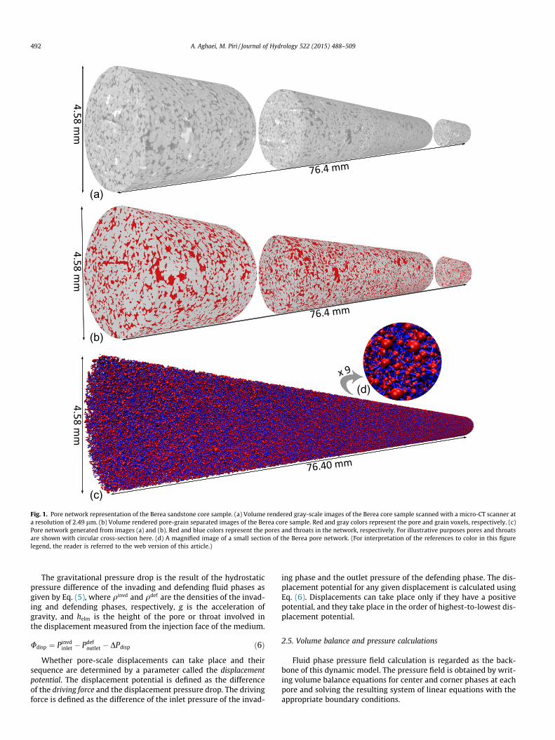
The dimensions and petrophysical properties of the Bentheimerand Berea networks are listed in Tables 3 and 4, respectively. Thepores and throats of our networks have rectangular, scalene trian-gular, and circular cross sections. Fig. 1(a) shows a volume ren-dered gray scale image of the Berea sandstone core sample. Thisgray scale image is segmented using the histogram thresholdingtechnique producing a pore-grain separated labeled image seenin Fig. 1(b), where red and gray colors represent the pore and grainvoxels, respectively. The gray-scale and pore-grain separatedimages are used to construct a pore network representative ofthe Berea core sample, as shown in Fig. 1(c). In the pore networkimage, pores and throats are shown with red spheres and blue cyl-inders, respectively. Fig. 1(d) shows a magnified image of a smallsection of the Berea pore network.
2.2. Model assumptions
In this model, fluids are assumed to be Newtonian, incompress-ible, and immiscible. Fluid–fluid interfaces are assumed to be sharpwith no diffusion taking place between two phases. Fluid flowinside pores and throats is described by Stokes or creeping flow.The clay inside the pore-space is assumed to be fully saturatedwith immobile water.
2.3. Pore-scale displacements
A series of pore-scale fluid displacements are carried out in thepore network to simulate two-phase flow displacements in porousmedia. Three fundamental types of pore-scale displacement mech-anisms included in this dynamic model are piston-like, pore-bodyfilling (cooperative filling), and snap-off.
The simulations start with fully water saturated pores andthroats where all possible displacements from the inlet have beenadded to the system. Displacements occur in the order of highest-to-lowest displacement potential (see Section 2.4) that takes intoaccount the effects of capillary, viscous, and gravitational pressuredrops. After each displacement, new displacements are added tothe system based on the access of fluid phases to each other.
Table 3Properties of the pore network representative of the Bentheimer sandstone coresample used in Experiment 1.
Item Throats Pores Total
Number 306,825 131,346 438,171Porosity excl. clay (%) 9.697 13.631 23.328Porosity incl. clay (%) 11.261 13.772 25.033Absolute Permeability (mD) 2716Length (mm) 12.977Diameter (mm) 4.972Minimum coordination number 0Maximum coordination number 150Average coordination number 4.622Minimum radius (lm) 0.28 0.30 0.28Maximum radius (lm) 101.00 148.48 148.48Average radius (lm) 13.71 25.96 17.38Average shape factor 0.042 0.046 0.044Triangular cross sections (%) 79.790 70.665 77.055Square cross sections (%) 19.590 28.959 22.399Circular cross sections (%) 0.620 0.376 0.546Connected to the inlet 3363 0 3363Connected to the outlet 3248 0 3248Isolated clusters 45Isolated 143 446 589
2.4. Displacement pressure drop and sequence
The multiphase flow behavior in porous media is determined bythe interlinked effects of capillary, viscous, and gravity forces.Therefore it is essential to include the effects of these three basicforces in the model. In this work, this is achieved by combiningthe capillary, viscous, and gravitational pressure drops of a dis-placement into a new parameter called the displacement pressuredrop as given by Eq. (1).
DPdisp ¼ DPcap þ DPvisc þ DPgrav ð1Þ
Nc ¼lmr
ð2Þ
Bo ¼ DqgL2
rð3Þ
The contribution of each term in the displacement pressuredrop to its total value depends on the capillary and Bond numbers(Eqs. (2) and (3)). In the cases where the capillary and Bond num-bers are both very low, capillary pressure dominates the flowbehavior in porous media. However by increasing the capillaryand Bond numbers the contributions of viscous and gravitationalpressure drops, respectively, become more significant.
For piston-like displacements we use the Mayer–Stowe–Prin-cen (MSP) method to calculate the capillary pressure drop of dis-placements (Mayer and Stowe, 1965; Princen, 1969a,b, 1970;Øren et al., 1998; Piri and Blunt, 2005a). In this method, an energybalance equation is written for the fluid configuration changesassociated with a pore-scale displacement. By assuming the equi-librium conditions at constant temperature and combining theresultant equation with the Young–Laplace equation, the capillarypressure drop during a fluid configuration change is obtained.
DPvisc ¼ ðPinvdinlet � Pinvd
elm Þ þ ðPdefelm � Pdef
outletÞ ð4Þ
The viscous pressure drop occurs due to the friction between lay-ers of fluid that move with different velocities. We calculate the vis-cous pressure drop for both the invading and defending fluid phases.For the invading fluid phase the viscous pressure drop is calculatedfrom the inlet of the pore network to the displacement location, andfor the defending fluid phase, it is calculated from the displacementlocation to the outlet of the pore network as written in Eq. (4).
DPgrav ¼ ðqinvd � qdefÞghelm ð5Þ
76.4 mm
76.4 mm
76.40 mm
x 9
(d)
(b)
(c)
(a)
4.58 mm
4.58 mm
4.58 mm
Fig. 1. Pore network representation of the Berea sandstone core sample. (a) Volume rendered gray-scale images of the Berea core sample scanned with a micro-CT scanner ata resolution of 2.49 lm. (b) Volume rendered pore-grain separated images of the Berea core sample. Red and gray colors represent the pore and grain voxels, respectively. (c)Pore network generated from images (a) and (b). Red and blue colors represent the pores and throats in the network, respectively. For illustrative purposes pores and throatsare shown with circular cross-section here. (d) A magnified image of a small section of the Berea pore network. (For interpretation of the references to color in this figurelegend, the reader is referred to the web version of this article.)
492 A. Aghaei, M. Piri / Journal of Hydrology 522 (2015) 488–509
The gravitational pressure drop is the result of the hydrostaticpressure difference of the invading and defending fluid phases asgiven by Eq. (5), where qinvd and qdef are the densities of the invad-ing and defending phases, respectively, g is the acceleration ofgravity, and helm is the height of the pore or throat involved inthe displacement measured from the injection face of the medium.
Udisp ¼ Pinvdinlet � Pdef
outlet � DPdisp ð6Þ
Whether pore-scale displacements can take place and theirsequence are determined by a parameter called the displacementpotential. The displacement potential is defined as the differenceof the driving force and the displacement pressure drop. The drivingforce is defined as the difference of the inlet pressure of the invad-
ing phase and the outlet pressure of the defending phase. The dis-placement potential for any given displacement is calculated usingEq. (6). Displacements can take place only if they have a positivepotential, and they take place in the order of highest-to-lowest dis-placement potential.
2.5. Volume balance and pressure calculations
Fluid phase pressure field calculation is regarded as the back-bone of this dynamic model. The pressure field is obtained by writ-ing volume balance equations for center and corner phases at eachpore and solving the resulting system of linear equations with theappropriate boundary conditions.

i, Water j, Water ij, Water
Config. 1
i, Oil j, Oil ij, Oil
Config. 4
i, Oil j, Oil ij, Water
Config. 6
i, Oil j, Water ij, Oil
Config. 3
i, Oil j, Water ij, Water
Config. 2
i, Water j, Water ij, Oil
Config. 5
Fig. 2. All possible fluid configurations in an assembly of two pores and a throat. Pores and throats are shown with circles and rectangles for illustrative purposes only. Theycan have angular cross-sections and contain a center as well as a corner phase. Only the center phases are illustrated here. The corners will contain water if the elements areangular. The dotted curvatures show the Main Terminal Menisci (MTM’s) present between the wetting and non-wetting phases.
A. Aghaei, M. Piri / Journal of Hydrology 522 (2015) 488–509 493
Xn
j¼1
qij ¼ 0 ð7Þ
Eq. (7) gives the volume balance for pore i where qij is the flow ratebetween pores i and j, and n is the coordination number of pore i.For a pore that contains the non-wetting phase at its center andthe wetting phase at its corners, this equation is written twice, oncefor the center phase and another time for the corner phase.
There are six possible configurations of two fluid phases in anassembly of two pores and a throat as shown in Fig. 2. Pores andthroats are shown by circles and cylinders for illustrative purposesonly. They can have angular cross sections and contain center andcorner phase locations. In configurations 1 and 4, no Main TerminalMeniscus (MTM) exists between pores i and j, therefore the singlephase flow equations are written for the center and corner phasesof these configurations.
qpij ¼ gp
ijðPpi � Pp
j Þ ð8Þ1gp
ij
¼ 1gp
pore;i
þ 1gp
throat;ij
þ 1gp
pore;j
ð9Þ
Eq. (8) gives the corner flow and single-phase center flow, where gpij
is the equivalent conductance of fluid phase p between pores i and j,and Pp
i and Ppj are pressures of fluid phase p in pores i and j, respec-
tively. gpij is calculated through Eq. (9).
Pconfig:2c ¼ Po
i �Pwj ð10Þ
Udraconfig:2¼ Pconfig:2
c �Pdrac;ij ð11Þ
Uimbconfig:2¼ Pimb
c;i �Pconfig:2c ð12Þ
qij¼gce
ij ðPnwi �Pw
j �Pdrac;ij Þ if Udra
config:2 >Uimbconfig:2 and Udra
config:2 >0
gceij ðP
nwi �Pw
j �Pimbc;i Þ if Uimb
config:2 >Udraconfig:2 and Uimb
config:2 >0
0 if Udraconfig:2 < 0 and Uimb
config:2 <0
8>><>>:
ð13Þ
In configurations where one or two MTM’s exist between twopores (see Fig. 2), two-phase flow equations are used to describethe center flow between the pores. The center flow equations forconfiguration 2 will be discussed here. In configuration 2, oneoil–water MTM is located at the entrance of throat ij. The MTMcan either move into throat ij and cause a drainage-type flow, orretreat into pore i and cause an imbibition-type flow dependingon the local capillary pressure and threshold capillary pressuresof pore i and throat ij. Local capillary pressure for configuration 2is written as the difference of oil pressure in pore i and water pres-sure in pore j (Eq. (10)). The potentials for two possible types of theMTM movement in configuration 2 are given by Eqs. (11) and (12),
where Pdrac;ij is the drainage threshold capillary pressure of throat ij
and Pimbc;i is the imbibition threshold capillary pressure of pore i.
As written in Eq. (13), if the drainage potential of the MTM is posi-tive and greater than its imbibition potential, then a drainage-typeflow will be considered for the MTM. However, if the imbibitionpotential is positive and greater than the drainage potential, thenan imbibition-type flow will be considered for the MTM. In caseswhere both potentials are negative there will be no two-phase flowtaking place between pores i and j.
1gce
ij
¼ 1gnw
pore;iþ 1
gwthroat;ij
þ 1gw
pore;jð14Þ
The equivalent center flow conductance, gceij , in configuration 2,
is calculated through Eq. (14). The center flow conductances arecalculated by using the equations proposed by Øren et al. (1998)and Patzek and Silin (2001), while the corner flow conductancesare calculated by equations proposed by Hui and Blunt (2000).
The resultant system of linear equations is solved by using theMUMPS package, which is a massively parallel sparse matrix solver(Amestoy et al., 2001, 2006).
2.6. Boundary conditions
In order to replicate the experimental conditions during simula-tions and to be able to study steady-state two-phase flow processes,wetting and non-wetting fluids are injected simultaneously at con-stant flow rates from the inlet of the medium. This is similar to thework by Hashemi et al. (1998, 1999b,a) in which both the wettingand non-wetting fluids act as the invader and the defender. In ourmodel, drainage and imbibition processes are simulated by chang-ing the inlet flow rates. The direction in which the inlet flow rateschange determines the type of two-phase flow process we simulate.
Xn
j¼1
qpij ¼ qp
inlet ð15Þ
Material balance is written for the inlet as shown in Eq. (15)where qp
inlet is the flow rate of phase p at the inlet. Pressures of wet-ting and non-wetting phases at the inlet are obtained by solvingthe material balance equations.
At the outlet of the medium, constant pressure boundary condi-tions are enforced. Since the local capillary pressure at the porescale cannot be zero, a non-zero capillary pressure is enforced atthe outlet. The outlet capillary pressure has the value below whichno network-spanning cluster of the non-wetting phase can exist inthe system. During drainage, when the non-wetting phase reachesthe outlet of the network, the pressures of the wetting and

494 A. Aghaei, M. Piri / Journal of Hydrology 522 (2015) 488–509
non-wetting fluids are averaged in a partition of the network adja-cent to the outlet, and capillary pressure is determined in that par-tition. This capillary pressure is set as the outlet capillary pressure.However, if the capillary number is high, the outlet capillary pres-sure can be overestimated using this method. Therefore, the capil-lary pressure set at the outlet is reduced gradually in smallincrements to find the value below which the connection of thenon-wetting phase to the outlet is lost completely. This criticalvalue is set as the outlet capillary pressure. This procedure is per-formed automatically by the model as soon as the breakthrough ofthe non-wetting phase occurs. The outlet capillary pressure is keptconstant during the simulations. One should note that the valuesset as the outlet capillary pressure are insignificant compared tothe macroscopic pressure drops along the network.
2.7. Corner interface handling
The location of Arc Menisci (AM’s) determine the area open tocorner and center flows and have a significant impact on pressurevalues and thereby relative permeabilities as well as other pre-dicted properties. This dynamic model allows the location ofAM’s to be updated based on the local capillary pressure and reced-ing and advancing contact angles. This is similar to the approachthat is often used in quasi-static network models in determiningthreshold capillary pressure for a snap-off displacement.
Pc ¼ rob1r1þ 1
r2
� �ð16Þ
When a new AM is formed in a pore element, its location isdetermined by calculating its distance from the apex of the cornerin which it is formed. The Young–Laplace equation (Eq. (16)) com-bined with a geometrical relationship is used to determine theapex-meniscus distance. After an AM is formed, the local capillarypressure might change due to changes in fluid phase pressure dis-tribution. The moving contact angle (hmov) is defined as the contactangle with which a fluid–fluid interface moves and it has a con-stant value during the interface movement. When the local capil-
movow
1r
2r
movow
1r
2r
advow
recow
hinow
hr
(a) (b)
Fig. 3. Corner interface adjustments based on changes in local capillary pressure.(a) The contact angle is equal to the receding contact angle. The corner interface, i.e.,AM moves towards the apex of the corner as the local capillary pressure increases.(b) The contact angle is greater than the receding contact angle. The corner interfacehinges as the local capillary pressure decreases.
lary pressure in a pore element changes, an AM in the poreelement will move only if its contact angle is equal to hmov, other-wise the AM will hinge and its contact angle will change by keep-ing a fixed apex-meniscus distance. As an example, as shown inFig. 3(a), if Pc increases and the contact angle is equal to the reced-ing contact angle, then the AM will move toward the corner apexwith a fixed contact angle. In Fig. 3(b), on the other hand, Pc
decreases, and the contact angle is lower than the advancing con-tact angle, therefore the AM will hinge away from the corner apexwith a fixed apex-meniscus distance.
2.8. Parallelization
The computational challenges in dynamic network modelshave limited the size of the mediums that were studied with pre-viously-developed models (see Tables 1 and 2). They have alsohindered studies of heterogeneous mediums at the pore scale.Calculating the fluid phase pressure field and updating thefluid–fluid interface locations and displacement potentials at eachtime step, and updating the continuity flags of neighboring fluidphase locations after each displacement are computationally themost demanding steps in this dynamic model. We take advantageof greater memory and computational resources available onmassive computer clusters. Data parallelism through three-dimensional domain decomposition was employed in designingthe parallel algorithms.
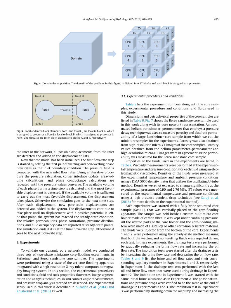
In Fig. 4, a domain decomposition scheme is illustrated, inwhich the domain of the problem is divided into, in this case,27 subdomains and each subdomain is assigned to one processor.In this work, the pore network is divided into multiple blocksbased on the availability of the computational resources, and eachblock is assigned to one processor. The pores and throats whosecenter coordinates lie inside the boundaries of a block are consid-ered as local elements to that block and their information isstored on the memory of the processor assigned to that block.The computations related to a pore or throat are done by the pro-cessor to which the element is local. Consider two neighboringblocks A and B as shown in Fig. 5. Pore i and throat ij are localto block A, which is assigned to processor a, and pore j is localto block B, which is assigned to processor b. Processor a is respon-sible for computations related to pore i and throat ij, and proces-sor b is responsible for computations related to pore j. However,during some computations, processors a and b might also needthe information related to pore j and throat ij, respectively. There-fore pore j and throat ij are considered as inter-block elements toblocks A and B, respectively, and part of their information needsto be stored in the memory of their respective processors as well.The information related to inter-block elements such as fluidphase occupancy and pressures needs to be communicated duringsimulations between neighboring processors. MPI (Message Pass-ing Interface) (Gabriel et al., 2004) libraries are used to carry outcommunications between processors in this model.
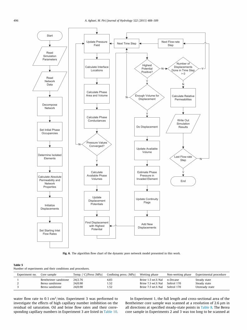
2.9. The model algorithm
The general outline of the model is explained in this section.Algorithm flow chart of the model is presented in Fig. 6. The firststep is reading the simulation parameters and the network dataand decomposing it among the available processors. Then, the ini-tial fluid phase is assigned to the pores and throats and the isolatedelements are detected in the pore network. A parallel clusteringalgorithm is developed for the cluster detection in a decomposeddomain. Next, the absolute permeability and porosity of the porenetwork are calculated. By examining the elements connected to
Domain
CPU 1
CPU 2
CPU 3
CPU 4
CPU 5
CPU 6
CPU 9
CPU 8
CPU 7
16 17 18 25 26 27
12
15
18
21
24
27
Fig. 4. Domain decomposition. The domain of the problem, in this figure, is divided into 27 blocks and each block is assigned to a processor.
Block A Block B
CPU a
Pore i Pore j Throat ij
CPU b
Fig. 5. Local and inter-block elements. Pore i and throat ij are local to block A, whichis assigned to processor a. Pore j is local to block B, which is assigned to processor b.Pore j and throat ij are inter-block elements to blocks A and B, respectively.
A. Aghaei, M. Piri / Journal of Hydrology 522 (2015) 488–509 495
the inlet of the network, all possible displacements from the inletare detected and added to the displacement lists.
Now that the model has been initialized, the first flow-rate stepis started by setting the first pair of wetting and non-wetting phaseflow rates as the inlet boundary condition. The pressure field iscomputed with the new inlet flow rates. Using an iterative proce-dure the pressure calculation, corner interface update, area-vol-ume calculations, and phase conductance calculations arerepeated until the pressure values converge. The available volumeof each phase during a time step is calculated and the most favor-able displacement is detected. If the available volume is sufficientto carry out the most favorable displacement, the displacementtakes place. Otherwise the simulation goes to the next time step.After each displacement, new pore-scale displacements aredetected and added to the system. The displacements continue totake place until no displacement with a positive potential is left.At that point, the system has reached the steady-state condition.The relative permeabilities, phase saturations, pressure distribu-tions, and fluid occupancy data are reported at steady-state points.The simulation ends if it is at the final flow-rate step. Otherwise itgoes to the next flow-rate step.
3. Experiments
To validate our dynamic pore network model, we conductedthree sets of two-phase miniature core-flooding experiments inBetheimer and Berea sandstone core samples. The experimentswere performed using a state-of-the-art core-flooding apparatusintegrated with a high-resolution X-ray micro-computed tomogra-phy imaging system. In this section, the experimental proceduresand conditions, fluid and rock properties, flow rates, image segmen-tation and analysis techniques, in situ contact angle measurements,and pressure drop analysis method are described. The experimentalsetup used in this work is described in Alizadeh et al. (2014) andKhishvand et al. (2015) as well.
3.1. Experimental procedures and conditions
Table 5 lists the experiment numbers along with the core sam-ples, experimental procedure and conditions, and fluids used inthis study.
Dimensions and petrophysical properties of the core samples arelisted in Table 6. Fig. 7 shows the Berea sandstone core sample usedin this work along with its pore network representation. An auto-mated helium porosimeter–permeameter that employs a pressuredecay technique was used to measure porosity and absolute perme-ability of a large Bentheimer core sample from which we cut theminiature samples for the experiments. Porosity was also obtainedfrom high-resolution micro-CT images of the core samples. Porosityvalues obtained from the helium porosimeter–permeameter andhigh-resolution micro-CT images were in agreement. Brine perme-ability was measured for the Berea sandstone core sample.
Properties of the fluids used in the experiments are listed inTable 7. Viscosity measurements were performed at the experimen-tal temperature and pressure conditions for each fluid using an elec-tromagnetic viscometer. Densities of the fluids were measured atthe experimental temperature and ambient pressure conditionsusing a DMA 5000 density meter that utilizes the oscillating U-tubemethod. Densities were not expected to change significantly at theexperimental pressures of 0.90 and 2.76 MPa. IFT values were mea-sured at the experimental temperature and pressure conditionsusing a high pressure pendent drop technique (see Saraji et al.(2013) for more details on the experimental method).
Each experiment was started with a fully brine saturated coresample (Sw = 1), that was vertically placed in the core-floodingapparatus. The sample was held inside a custom-built micro coreholder made of carbon fiber. It was kept under confining pressure.All the wetted parts of the core holder and the core-flooding sys-tem were made of Hastelloy or other corrosion resistant material.The fluids were injected from the bottom of the core. Experiments1 and 2 were performed using the steady-state method meaningthat both the wetting and non-wetting fluids were injected duringeach test. In these experiments, the drainage tests were performedby gradually reducing the brine flow rate and increasing the oilflow rate. The imbibition tests were started after the drainage testsby increasing the brine flow rate and decreasing the oil flow rate.Tables 8 and 9 list the brine and oil flow rates and their corre-sponding capillary numbers in Experiments 1 and 2, respectively.In Experiment 3, the drainage test was performed with the lastoil and brine flow rates that were used during drainage in Experi-ment 2. The imbibition test in Experiment 3 was started with thesame initial brine saturation as in Experiment 2. The phase satura-tions and pressure drops were verified to be the same at the end ofdrainage in Experiments 2 and 3. The imbibition test in Experiment3 was performed by shutting down the oil pump and increasing the
Start
Read Simulation Parameters
Read Network
Data
Decompose Network
Set Initial Phase Occupancies
Determine Isolated Elements
Calculate Absolute Permeability and
Network Properties
Initialize Displacements
Set Starting Inlet Flow Rates
Calculate Phase Conductances
Update Pressure Field
Calculate Interface Locations
Calculate Phase Area and Volume
Pressure Values Converged?
Calculate Available Phase
Volumes
Update Displacement
Potentials
Highest Potential Positive?
Find Displacement with Highest
Potential
Enough Volume for Displacement
Do Displacement
Update Available Volume
Estimate Phase Pressure in
Invaded Element
Update Continuity Flags
Add New Displacements
Calculate Relative Permeabilites
Write Out Simulation
Results
Last Flow-rate Step
End
Number of Displacements
Done in Time Step > 0
N
Y
Y
Next Time Step
Y
Y
Y
Next Flow-rate Step
N
N
N
N
Fig. 6. The algorithm flow chart of the dynamic pore network model presented in this work.
Table 5Number of experiments and their conditions and procedures.
Experiment no. Core sample Temp. (�C)/Press (MPa) Confining press. (MPa) Wetting phase Non-wetting phase Experimental procedure
1 Bentheimer sandstone 24/2.76 4.83 Brine 1.5 wt.% NaI n-Decane Steady state2 Berea sandstone 24/0.90 1.52 Brine 7.5 wt.% NaI Soltrol 170 Steady state3 Berea sandstone 24/0.90 1.52 Brine 7.5 wt.% NaI Soltrol 170 Unsteady state
496 A. Aghaei, M. Piri / Journal of Hydrology 522 (2015) 488–509
water flow rate to 0:1 cm3=min. Experiment 3 was performed toinvestigate the effects of high capillary number imbibition on theresidual oil saturation. Oil and brine flow rates and their corre-sponding capillary numbers in Experiment 3 are listed in Table 10.
In Experiment 1, the full length and cross-sectional area of theBentheimer core sample was scanned at a resolution of 2.6 lm inall directions at specified steady-state points in Table 8. The Bereacore sample in Experiments 2 and 3 was too long to be scanned at
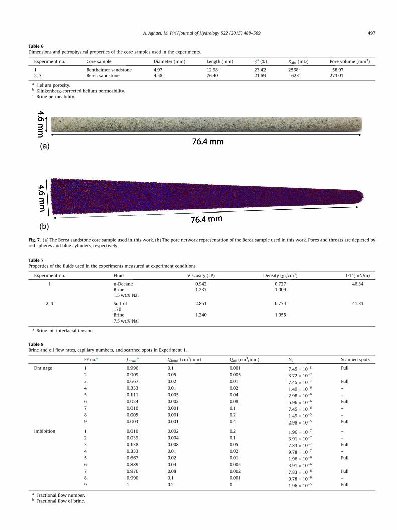
Table 6Dimensions and petrophysical properties of the core samples used in the experiments.
Experiment no. Core sample Diameter (mm) Length (mm) /a (%) Kabs (mD) Pore volume (mm3)
1 Bentheimer sandstone 4.97 12.98 23.42 2568b 58.972, 3 Berea sandstone 4.58 76.40 21.69 623c 273.01
a Helium porosity.b Klinkenberg-corrected helium permeability.c Brine permeability.
(a)
(b)Fig. 7. (a) The Berea sandstone core sample used in this work. (b) The pore network representation of the Berea sample used in this work. Pores and throats are depicted byred spheres and blue cylinders, respectively.
Table 7Properties of the fluids used in the experiments measured at experiment conditions.
Experiment no. Fluid Viscosity (cP) Density (gr/cm3) IFTa(mN/m)
1 n-Decane 0.942 0.727 46.34Brine1.5 wt.% NaI
1.237 1.009
2, 3 Soltrol 2.851 0.774 41.33170Brine7.5 wt.% NaI
1.240 1.055
a Brine–oil interfacial tension.
Table 8Brine and oil flow rates, capillary numbers, and scanned spots in Experiment 1.
FF no.a f brineb Qbrine (cm3/min) Qoil (cm3/min) Nc Scanned spots
Drainage 1 0.990 0.1 0.001 7:45� 10�8 Full
2 0.909 0.05 0.005 3:72� 10�7 –
3 0.667 0.02 0.01 7:45� 10�7 Full
4 0.333 0.01 0.02 1:49� 10�6 –
5 0.111 0.005 0.04 2:98� 10�6 –
6 0.024 0.002 0.08 5:96� 10�6 Full
7 0.010 0.001 0.1 7:45� 10�6 –
8 0.005 0.001 0.2 1:49� 10�5 –
9 0.003 0.001 0.4 2:98� 10�5 Full
Imbibition 1 0.010 0.002 0.2 1:96� 10�7 –
2 0.039 0.004 0.1 3:91� 10�7 –
3 0.138 0.008 0.05 7:83� 10�7 Full
4 0.333 0.01 0.02 9:78� 10�7 –
5 0.667 0.02 0.01 1:96� 10�6 Full
6 0.889 0.04 0.005 3:91� 10�6 –
7 0.976 0.08 0.002 7:83� 10�6 Full
8 0.990 0.1 0.001 9:78� 10�6 –
9 1 0.2 0 1:96� 10�5 Full
a Fractional flow number.b Fractional flow of brine.
A. Aghaei, M. Piri / Journal of Hydrology 522 (2015) 488–509 497

Table 9Brine and oil flow rates, capillary numbers, and scanned spots in Experiment 2.
FF no.a f brineb Qbrine (cm3/min) Qoil (cm3/min) Nc Scanned spots
Drainage 1 0.952 0.1 0.005 5:07� 10�7 1, 2, 3
2 0.833 0.05 0.01 1:01� 10�6 2
3 0.5 0.02 0.02 2:03� 10�6 2
4 0.167 0.01 0.05 5:07� 10�6 2
5 0.048 0.005 0.1 1:01� 10�5 2
6 0.007 0.001 0.15 1:52� 10�5 1, 2, 3
Imbibition 1 0.038 0.002 0.05 2:40� 10�7 2
2 0.167 0.004 0.02 4:80� 10�7 2
3 0.444 0.008 0.01 9:60� 10�7 1, 2, 3
4 0.667 0.01 0.005 1:20� 10�6 2
5 0.909 0.02 0.002 2:40� 10�6 2
6 1 0.05 0 6:00� 10�6 1, 2, 3
a Fractional flow number.b Fractional flow of brine.
Table 10Brine and oil flow rates, capillary numbers, and scanned spots in Experiment 3.
FF no.a Qbrine (cm3/min) Qoil (cm3/min) Nc Scanned spots
Drainage 1 0.001 0.15 1:52� 10�5 1, 2, 3
Imbibition 1 0.1 0 1:20� 10�5 1, 2, 3
2 0.15 0 1:80� 10�5 1, 2, 3
a Fractional flow number.
Table 11Scanned spots locations along the Berea core sample in Experiments 2 and 3.
Spot No. Middle of spot from inlet mm Spot length (mm)
1 11.07 4.412 35.90 4.413 67.55 4.41
498 A. Aghaei, M. Piri / Journal of Hydrology 522 (2015) 488–509
full length at every steady-state point. Therefore, certain locationsalong the Berea core were selected as scan spots. The location ofthese spots and their lengths and numbers are listed in Table 11.The Berea core in Experiments 2 and 3 was scanned at a resolutionof 2.49 lm, in all directions, at fractional flow steps and scan spotsspecified in Tables 9 and 10.
3.2. Steady-state criteria for experiments
During the experiments, after the brine and oil flow rates were setto their predetermined values, the pressure drop along the core sam-ple was monitored carefully. Four differential pressure transducerswith various ranges were used to measure the pressure drop alongthe cores. When the pressure drop reached a stable value, the lowerresolution scanning of the core sample was started. The core samplewas scanned repeatedly until the saturation difference between twoconsecutive scans was less than 1%. This would ensure the establish-ment of the steady-state condition. At that point, the core samplewas scanned with a higher resolution and the pressure drop datawere recorded for relative permeability calculations.
3.3. Micro-CT image segmentation and analysis
The micro-CT images of the core samples were analyzed usingthe Avizo� Fire software. A technique similar to the one used by
Alizadeh et al. (2014) and Khishvand et al. (2015) was used forthe analysis of the micro-CT images. The dry core samples werescanned to obtain reference images before the flow experimentswere started (see Fig. 8(a)). First, the non-local means filter wasapplied to the reference images to reduce the noise. The referenceimages were then segmented using histogram thresholding tech-nique as shown in Fig. 8 (b).
The analysis of the wet images obtained during the flow exper-iments (see Fig. 8(c)) was started, similar to dry images, by apply-ing the non-local means filter. Then, the wet images wereregistered with the dry images and were multiplied by the binarypore-grain separated images to separate the pore space and grains.The resulting images were then segmented for the separation ofthe oil and brine phases (see Fig. 8(d)). Arithmetic operations wereperformed on these labeled images to obtain average saturationsand saturation profiles along the core sample.
3.4. In-situ contact angle measurements
The micro-CT images obtained during the two-phase flowexperiments were used to measure the contact angles betweenthe wetting and non-wetting phases in the pore space. This is sim-ilar to the technique used by Andrew et al. (2014). First a corner ofa pore containing the brine and oil phases was selected. Then thepoint where the brine-oil interface line intersects the solid surfacewas detected. At that point, two lines one tangent to the solid sur-face and the other one tangent to the brine-oil interface weredrawn. The angle between these two lines through the brine phasegave the brine-oil contact angle at that corner. Fig. 9 shows in situcontact angle measurements in pore corners in the Berea sand-stone core during the experiments. Brine, oil, and grains aredepicted by colors blue, red, and gray, respectively. The green linesshow the tangents to the rock surface and the brine-oil interface atthe triple contact points.
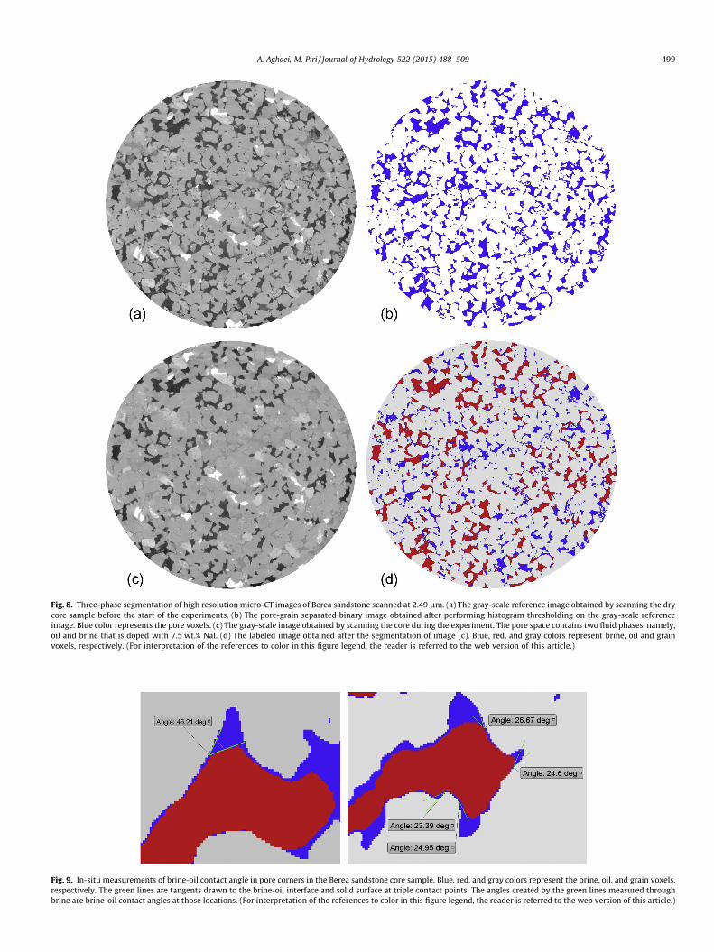
Fig. 8. Three-phase segmentation of high resolution micro-CT images of Berea sandstone scanned at 2.49 lm. (a) The gray-scale reference image obtained by scanning the drycore sample before the start of the experiments. (b) The pore-grain separated binary image obtained after performing histogram thresholding on the gray-scale referenceimage. Blue color represents the pore voxels. (c) The gray-scale image obtained by scanning the core during the experiment. The pore space contains two fluid phases, namely,oil and brine that is doped with 7.5 wt.% NaI. (d) The labeled image obtained after the segmentation of image (c). Blue, red, and gray colors represent brine, oil and grainvoxels, respectively. (For interpretation of the references to color in this figure legend, the reader is referred to the web version of this article.)
Fig. 9. In-situ measurements of brine-oil contact angle in pore corners in the Berea sandstone core sample. Blue, red, and gray colors represent the brine, oil, and grain voxels,respectively. The green lines are tangents drawn to the brine-oil interface and solid surface at triple contact points. The angles created by the green lines measured throughbrine are brine-oil contact angles at those locations. (For interpretation of the references to color in this figure legend, the reader is referred to the web version of this article.)
A. Aghaei, M. Piri / Journal of Hydrology 522 (2015) 488–509 499

Table 12In-situ brine-oil contact angles measured in the Bentheimer and Berea sandstone samples during experiments and used in simulations.
Core sample Exp/Sim no. Process/Type Average hAM Min hAM Max hAM
Bentheimer sandstone
Exp 1 Drainage 22.83 10.81 32.33Imbibition 28.22 19.83 42.11
Sim 1 Receding 22 12 32Advancing 45 35 55
Berea sandstone
Exp 2, 3 Drainage 15.51 6.37 26.57Imbibition 35.59 7.83 56.14
Sim 2, 3 Receding 16 6 26Advancing 50 40 60
500 A. Aghaei, M. Piri / Journal of Hydrology 522 (2015) 488–509
Table 12 lists the average, minimum, and maximum brine-oilcontact angles measured at multiple points in the Bentheimerand Berea sandstone core samples during drainage and imbibitionprocesses of Experiments 1, 2, and 3. These values were used inidentifying the receding and advancing brine-oil contact angle dis-tributions in the Bentheimer and Berea pore networks in the sim-ulations presented here. The average, minimum, and maximumvalues of brine-oil contact angle distributions in the Bentheimerand Berea pore networks are also listed in Table 12 for comparison.
3.5. Fluid phase potential difference
In the experiments, the core sample was placed vertically andthe fluids were injected from the bottom of the core. Therefore,the effect of gravity needed to be included in the potential differ-ence in the Darcy’s equation. For this purpose, when the core sam-ple was fully saturated with brine, the injection pumps were shutdown and the pressure transducers were reset to zero. As a result,the value shown by the pressure transducers was the potential dif-ference for the brine phase and it needed to be corrected for the oilphase relative permeability calculations.
DUo ¼ DUb þ ðqb � qoÞgL ð17Þ
Eq. (17) was used to convert the pressure difference value read fromtransducers to the oil phase potential difference. In this equation,DUo and DUb are potential differences of oil and brine phasesrespectively, qb and qo are brine and oil densities, respectively, gis the acceleration of gravity, and L is the length of the core sample.After obtaining the potential differences for each phase, the relativepermeabilities were calculated using the Darcy’s equation.
4. Validation
In this section, first simulation procedures and conditions,steady-state criteria for simulations, and contact angle distribu-tions used in simulations are described. This is followed by thecomparison of simulation and experimental results.
4.1. Simulation procedures and conditions
The dynamic model was used to perform simulations in porenetworks constructed from high-resolution micro-computedtomography images of the core samples in which the experimentswere performed. The properties of the pore networks representa-tive of the Bentheimer and Berea core samples used in the experi-ments are presented in Tables 3 and 4, respectively. The propertiesof the fluids that were measured during the experiments and pre-sented in Table 7 were used in the simulations. The simulationswere performed using the same brine and oil flow rates used dur-ing the experiments. These flow rates and their corresponding cap-illary numbers are presented in Tables 8–10. For each experimentlisted in Table 5, there is an equivalent simulation with the samenumber.
The simulations were started with fully brine saturated porenetworks. The vertical orientation of the core sample was simu-lated by using the appropriate coordinates of pore elements asthe height in gravity pressure drop calculations (see Eq. (5)).
4.2. Steady-state criteria for simulations
In the simulations, the pore-scale displacements were carriedout in the order of highest-to-lowest displacement potential (seeSection 2.4). The displacements were carried out until no displace-ment with a positive potential was left in the system. At that point,the system had reached the steady-state condition for one set ofinlet flow rates. The simulation and experimental results are com-pared against each other at steady-state points.
4.3. Contact angles used in simulations
In-situ measurements of the brine-oil contact angles during theexperiments provided us with realistic estimations of contact angledistributions in the real rock pore space (see Section 3.4). The aver-age, minimum, and maximum values of the random distributionsof the receding and advancing contact angles used in the Bereaand Bentheimer pore networks are listed in Table 12. One shouldnote that the contact angles measured during drainage are reced-ing. However, the contact angles measured during imbibition areeither hinging or advancing and accordingly their average valuesare between receding and advancing contact angles. Therefore,the advancing contact angle values used in the simulations are lar-ger than the contact angles measured during imbibition.
4.4. Comparison with experimental data
Simulations 1, 2, and 3 were performed as the equivalents ofExperiments 1, 2, and 3, respectively. Simulation 1 that was per-formed in the Bentheimer sandstone network took about 15 h tocomplete on 64 processors with 2000 MHz speed. While Simula-tions 2 and 3 that were performed in the Berea sandstone networktook about 2 weeks to complete on 200 processors with 2000 MHzspeed. The experimental and simulation data presented here relateto steady-state conditions that were established at each fractionalflow point. We compare each simulation with the correspondingexperiment through local saturation points, fractional flow curves,and relative permeabilities.
4.4.1. Simulation 1In Experiment 1, the full cross section and length of the Benthei-
mer core sample was scanned at selected fractional flow numberslisted in Table 8 after the steady-state condition was achieved. Thescanning resolution was 2.6 lm in all directions. After eliminatingthe micro-CT images close to the inlet and outlet of the core samplethat were corrupted due to geometric penumbra and high noise,4000 two-dimensional slices along the core sample were obtainedfor each fractional flow point. These slices were then processed andsegmented. For brine saturation profile measurements, these 4000
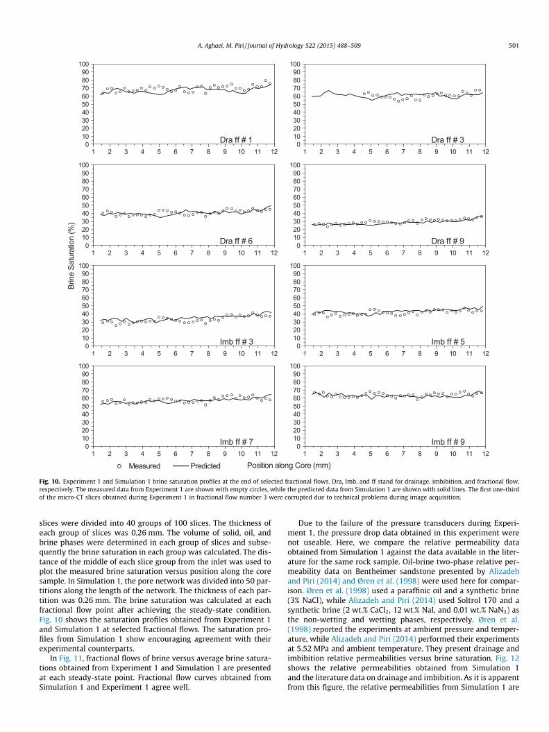
Fig. 10. Experiment 1 and Simulation 1 brine saturation profiles at the end of selected fractional flows. Dra, Imb, and ff stand for drainage, imbibition, and fractional flow,respectively. The measured data from Experiment 1 are shown with empty circles, while the predicted data from Simulation 1 are shown with solid lines. The first one-thirdof the micro-CT slices obtained during Experiment 1 in fractional flow number 3 were corrupted due to technical problems during image acquisition.
A. Aghaei, M. Piri / Journal of Hydrology 522 (2015) 488–509 501
slices were divided into 40 groups of 100 slices. The thickness ofeach group of slices was 0.26 mm. The volume of solid, oil, andbrine phases were determined in each group of slices and subse-quently the brine saturation in each group was calculated. The dis-tance of the middle of each slice group from the inlet was used toplot the measured brine saturation versus position along the coresample. In Simulation 1, the pore network was divided into 50 par-titions along the length of the network. The thickness of each par-tition was 0.26 mm. The brine saturation was calculated at eachfractional flow point after achieving the steady-state condition.Fig. 10 shows the saturation profiles obtained from Experiment 1and Simulation 1 at selected fractional flows. The saturation pro-files from Simulation 1 show encouraging agreement with theirexperimental counterparts.
In Fig. 11, fractional flows of brine versus average brine satura-tions obtained from Experiment 1 and Simulation 1 are presentedat each steady-state point. Fractional flow curves obtained fromSimulation 1 and Experiment 1 agree well.
Due to the failure of the pressure transducers during Experi-ment 1, the pressure drop data obtained in this experiment werenot useable. Here, we compare the relative permeability dataobtained from Simulation 1 against the data available in the liter-ature for the same rock sample. Oil-brine two-phase relative per-meability data on Bentheimer sandstone presented by Alizadehand Piri (2014) and Øren et al. (1998) were used here for compar-ison. Øren et al. (1998) used a paraffinic oil and a synthetic brine(3% NaCl), while Alizadeh and Piri (2014) used Soltrol 170 and asynthetic brine (2 wt.% CaCl2, 12 wt.% NaI, and 0.01 wt.% NaN3) asthe non-wetting and wetting phases, respectively. Øren et al.(1998) reported the experiments at ambient pressure and temper-ature, while Alizadeh and Piri (2014) performed their experimentsat 5.52 MPa and ambient temperature. They present drainage andimbibition relative permeabilities versus brine saturation. Fig. 12shows the relative permeabilities obtained from Simulation 1and the literature data on drainage and imbibition. As it is apparentfrom this figure, the relative permeabilities from Simulation 1 are
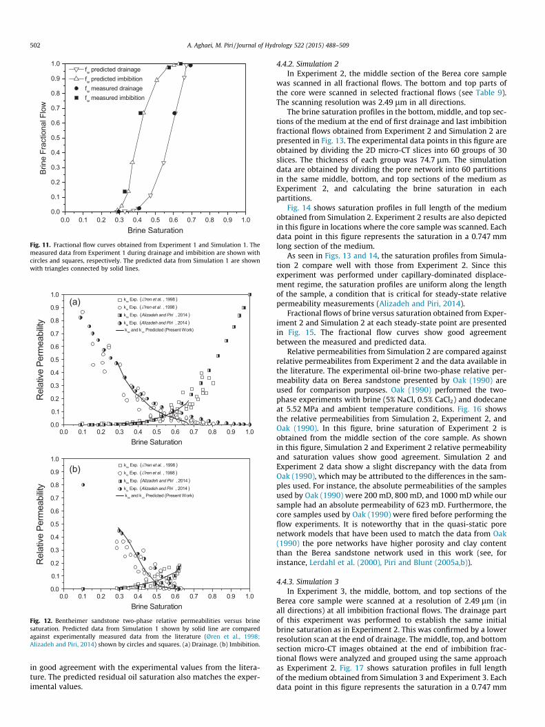
Fig. 11. Fractional flow curves obtained from Experiment 1 and Simulation 1. Themeasured data from Experiment 1 during drainage and imbibition are shown withcircles and squares, respectively. The predicted data from Simulation 1 are shownwith triangles connected by solid lines.
Fig. 12. Bentheimer sandstone two-phase relative permeabilities versus brinesaturation. Predicted data from Simulation 1 shown by solid line are comparedagainst experimentally measured data from the literature (Øren et al., 1998;Alizadeh and Piri, 2014) shown by circles and squares. (a) Drainage. (b) Imbibition.
502 A. Aghaei, M. Piri / Journal of Hydrology 522 (2015) 488–509
in good agreement with the experimental values from the litera-ture. The predicted residual oil saturation also matches the exper-imental values.
4.4.2. Simulation 2In Experiment 2, the middle section of the Berea core sample
was scanned in all fractional flows. The bottom and top parts ofthe core were scanned in selected fractional flows (see Table 9).The scanning resolution was 2.49 lm in all directions.
The brine saturation profiles in the bottom, middle, and top sec-tions of the medium at the end of first drainage and last imbibitionfractional flows obtained from Experiment 2 and Simulation 2 arepresented in Fig. 13. The experimental data points in this figure areobtained by dividing the 2D micro-CT slices into 60 groups of 30slices. The thickness of each group was 74.7 lm. The simulationdata are obtained by dividing the pore network into 60 partitionsin the same middle, bottom, and top sections of the medium asExperiment 2, and calculating the brine saturation in eachpartitions.
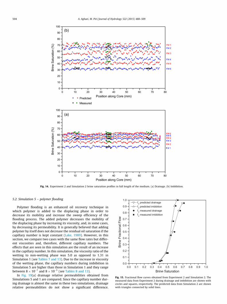
Fig. 14 shows saturation profiles in full length of the mediumobtained from Simulation 2. Experiment 2 results are also depictedin this figure in locations where the core sample was scanned. Eachdata point in this figure represents the saturation in a 0.747 mmlong section of the medium.
As seen in Figs. 13 and 14, the saturation profiles from Simula-tion 2 compare well with those from Experiment 2. Since thisexperiment was performed under capillary-dominated displace-ment regime, the saturation profiles are uniform along the lengthof the sample, a condition that is critical for steady-state relativepermeability measurements (Alizadeh and Piri, 2014).
Fractional flows of brine versus saturation obtained from Exper-iment 2 and Simulation 2 at each steady-state point are presentedin Fig. 15. The fractional flow curves show good agreementbetween the measured and predicted data.
Relative permeabilities from Simulation 2 are compared againstrelative permeabilites from Experiment 2 and the data available inthe literature. The experimental oil-brine two-phase relative per-meability data on Berea sandstone presented by Oak (1990) areused for comparison purposes. Oak (1990) performed the two-phase experiments with brine (5% NaCl, 0.5% CaCl2) and dodecaneat 5.52 MPa and ambient temperature conditions. Fig. 16 showsthe relative permeabilities from Simulation 2, Experiment 2, andOak (1990). In this figure, brine saturation of Experiment 2 isobtained from the middle section of the core sample. As shownin this figure, Simulation 2 and Experiment 2 relative permeabilityand saturation values show good agreement. Simulation 2 andExperiment 2 data show a slight discrepancy with the data fromOak (1990), which may be attributed to the differences in the sam-ples used. For instance, the absolute permeabilities of the samplesused by Oak (1990) were 200 mD, 800 mD, and 1000 mD while oursample had an absolute permeability of 623 mD. Furthermore, thecore samples used by Oak (1990) were fired before performing theflow experiments. It is noteworthy that in the quasi-static porenetwork models that have been used to match the data from Oak(1990) the pore networks have higher porosity and clay contentthan the Berea sandstone network used in this work (see, forinstance, Lerdahl et al. (2000), Piri and Blunt (2005a,b)).
4.4.3. Simulation 3In Experiment 3, the middle, bottom, and top sections of the
Berea core sample were scanned at a resolution of 2.49 lm (inall directions) at all imbibition fractional flows. The drainage partof this experiment was performed to establish the same initialbrine saturation as in Experiment 2. This was confirmed by a lowerresolution scan at the end of drainage. The middle, top, and bottomsection micro-CT images obtained at the end of imbibition frac-tional flows were analyzed and grouped using the same approachas Experiment 2. Fig. 17 shows saturation profiles in full lengthof the medium obtained from Simulation 3 and Experiment 3. Eachdata point in this figure represents the saturation in a 0.747 mm

Fig. 13. Experiment 2 and Simulation 2 brine saturation profiles in the bottom, middle, and top of the medium at the end of first drainage and last imbibition fractional flows.
A. Aghaei, M. Piri / Journal of Hydrology 522 (2015) 488–509 503
long section of the medium. Simulation 3 saturation profiles are ingood agreement with their experimental counterparts. Due to thedynamic effects caused by the higher capillary number duringimbibition (see Table 10), in Experiment 3 and Simulation 3, thereis a slight difference between brine saturation in the bottom, mid-dle, and top sections of the medium. The predicted residual oil sat-uration agrees closely with the experimental value.
5. Simulation of different processes
Having rigorously validated the dynamic model against theexperimental data, in this section, we use it to study other processes.Three simulations were conducted in the Bentheimer sandstonenetwork introduced earlier. All three simulations were performedwith the brine and oil flow rates used in Simulation 1 (see Table 8).However, different IFT and viscosity values were used in each simu-lation. Following the simulation numbering used in the previoussection, simulations in this section are numbered 4, 5, and 6. Proper-ties of the fluids and ranges of the capillary number in Simulations 4,5, and 6 are listed in Table 13. The contact angle distributions used inSimulation 1 (see Table 12) were used in Simulations 4, 5, and 6. Thesimulation results in this section are compared against the resultsfrom Simulation 1 with the purpose of investigating the effects oflow IFT and high viscosity of wetting phase on relative permeabili-ties, residual oil saturation, and fractional flow curves.
5.1. Simulation 4 – surfactant flooding
Surfactant flooding is an enhanced oil recovery technique that isused to increase recovery by reducing IFT between displacingphase and oil. By lowering IFT the capillary forces that are respon-
sible for trapping oil in the pore scale are reduced and the effect ofviscous forces becomes significant (Lake, 1989; Green and Willhite,1998). Simulation 4 was performed in order to investigate how alow IFT value might affect relative permeabilities and residual oilsaturation. The IFT value in this simulation was 1.0 mN/m asopposed to 46.34 mN/m in Simulation 1 (see Tables 7 and 13).Due to the reduced IFT value, the capillary numbers in Simulation4 are higher than those in Simulation 1 and they range between3� 10�6 and 1� 10�3 (see Tables 8 and 13).
As seen in Fig. 18, relative permeabilities of wetting and non-wetting phases in Simulation 4 are higher than those in Simulation1 for a given saturation. Furthermore, a wider range of saturation isobserved during drainage and imbibition in Simulation 4. Residualoil saturation in this simulation is 21.36%, which is 15.75% lowerthan that in Simulation 1 with a higher IFT.
In Simulation 4, due to the low IFT value used, the capillary pres-sure drop associated with pore-scale displacements becomes lowerand the viscous pressure drop becomes a more significant term in thedisplacement pressure drop (see Section 2.4). Therefore, pore-scaledisplacements take place in paths that result in lower viscous pres-sure drop. These flow paths can conduct the same flow rate withlower viscous pressure drop. In other words, there is less resistancein these flow paths. For this reason, higher relative permeabilities areobtained in Simulation 4 for a given saturation.
In this simulation, the rise in the capillary number makes the effectof viscous pressure drop more dominant. Therefore, the pore-scaledisplacements that are closer to the displacement front become morefavorable. Consequently, piston-like displacements close to the dis-placement front are favored over snap-off displacements ahead ofthe front. This change in the favored displacement type results in lesstrapping of the non-wetting phase. Therefore, in this simulation resid-ual oil saturation is lower than that in Simulation 1.
(b)
(a)
Fig. 14. Experiment 2 and Simulation 2 brine saturation profiles in full length of the medium. (a) Drainage. (b) Imbibition.
Fig. 15. Fractional flow curves obtained from Experiment 2 and Simulation 2. Themeasured data from Experiment 2 during drainage and imbibition are shown withcircles and squares, respectively. The predicted data from Simulation 2 are shownwith triangles connected by solid lines.
504 A. Aghaei, M. Piri / Journal of Hydrology 522 (2015) 488–509
5.2. Simulation 5 – polymer flooding
Polymer flooding is an enhanced oil recovery technique inwhich polymer is added to the displacing phase in order todecrease its mobility and increase the sweep efficiency of theflooding process. The added polymer decreases the mobility ofthe displacing phase by increasing its viscosity, and, in some cases,by decreasing its permeability. It is generally believed that addingpolymer by itself does not decrease the residual oil saturation if thecapillary number is kept constant (Lake, 1989). However, in thissection, we compare two cases with the same flow rates but differ-ent viscosities and, therefore, different capillary numbers. Theeffects that are seen in this simulation are the result of an increasein the capillary number. In this simulation, the viscosity ratio of thewetting to non-wetting phase was 5.0 as opposed to 1.31 inSimulation 1 (see Tables 7 and 13). Due to the increase in viscosityof the wetting phase, the capillary numbers during imbibition inSimulation 5 are higher than those in Simulation 1 and they rangebetween 8� 10�7 and 8� 10�5 (see Tables 8 and 13).
In Fig. 19(a) drainage relative permeabilities obtained fromSimulations 5 and 1 are compared. Since the capillary number dur-ing drainage is almost the same in these two simulations, drainagerelative permeabilities do not show a significant difference.

(a)
(b)
Fig. 16. Berea sandstone relative permeabilities versus brine saturation. Thepredicted data from Simulation 2 are compared against the measured data fromExperiment 2 and the experimental data by Oak (1990). (a) Drainage. (b) Imbibition.
A. Aghaei, M. Piri / Journal of Hydrology 522 (2015) 488–509 505
However, drainage steady-state points in Simulation 5 are estab-lished at lower wetting-phase saturations than those in Simulation1 for a given fractional flow. This can be attributed to the fact thatthe higher viscosity of the wetting phase in Simulation 5 increasesthe viscous pressure drop of the wetting phase and makes it moredifficult for oil to displace the wetting phase with the same flowrates as in Simulation 1.
As seen in Fig. 19(b), wetting-phase relative permeability doesnot show a big difference in Simulations 5 and 1. Oil relative
Fig. 17. Experiment 3 and Simulation 3 brine saturation profiles
permeability, however, is greater in Simulation 5 for a given satu-ration. Furthermore, the residual oil saturation in Simulation 5 is24.10%, which is 13.01% lower than residual oil saturation in Sim-ulation 1. Because of the higher wetting-phase-to-oil viscosityratio in Simulation 5, the flow pattern becomes more stable duringimbibition (Lenormand et al., 1988), meaning that the wetting-phase-to-oil displacements closer to the inlet are favored. There-fore, piston-like displacements closer to the inlet are favored oversnap-off displacements ahead of the displacement front. Thechange in the flow pattern results in less trapping of oil. Therefore,oil relative permeability is higher and residual oil saturation islower in Simulation 5.
5.3. Simulation 6 – surfactant-polymer flooding
Polymers are sometimes used in surfactant flooding in order toincrease the sweep efficiency of the process by lowering the mobil-ity of the displacing phase (Lake, 1989). Simulation 6 was per-formed to study the combined effect of low IFT and highviscosity of the wetting phase on relative permeabilities and resid-ual oil saturation. Due to the low IFT value and high viscosity of thewetting-phase, the capillary numbers in Simulation 6 are higherthan those in Simulations 1, 4, and 5 and they range between4� 10�6 and 4� 10�3 (see Tables 8 and 13).
As shown in Fig. 20(a), the dynamic effects observed duringdrainage in Simulation 4 are present and more significant in Sim-ulation 6. Saturation ranges in Simulations 4 and 6 are almost iden-tical during drainage. However, steady-state points are establishedat different saturations in these simulations for a given fractionalflow. Wetting-phase relative permeability is higher in Simulation6 for a given saturation. Oil relative permeability is higher in earlystages and then it becomes lower in late drainage.
Because in Simulation 6 viscosity ratio of wetting phase to oil is5.0, during drainage, oil has an unstable front (Lenormand et al.,1988). The low IFT value and the high viscosity of the wettingphase in this simulation makes the wetting-phase viscous pressuredrop the dominant force in displacements. Therefore, oil-to-wet-ting-phase displacements that are closer to the outlet are pre-ferred. In other words, displacements tend to take place in thepaths that cause the least wetting-phase viscous pressure drop.However, these displacement paths do not necessarily have theleast resistance to oil. Furthermore, there may be some un-sweptbanks of water that would cause more viscous pressure drop inoil flow. Additionally, the high viscosity of the wetting phaseincreases the wetting-phase pressure in the corners and keepsthe wetting layers thick in Simulation 6. Because of the above-mentioned reasons, drainage wetting-phase relative permeability
in full length of the medium in imbibition fractional flows.
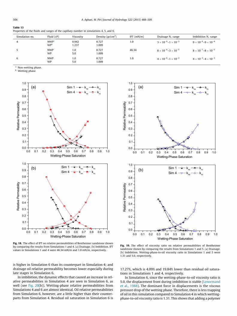
Table 13Properties of the fluids and ranges of the capillary number in simulations 4, 5, and 6.
Simulation no. Fluid (cP) Viscosity Density (gr/cm3) IFT (mN/m) Drainage Nc range Imbibition Nc range
4 NWPa 0.942 0.727 1.0 3� 10�6–1� 10�3 9� 10�6–9� 10�4
WPb 1.237 1.009
5 NWP 1.0 0.727 46.34 8� 10�8–3� 10�5 8� 10�7–8� 10�5
WP 5.0 1.009
6 NWP 1.0 0.727 1.0 4� 10�6–1� 10�3 4� 10�5–4� 10�3
WP 5.0 1.009
a Non-wetting phase.b Wetting phase.
(a)
(b)
Fig. 18. The effect of IFT on relative permeabilities of Bentheimer sandstone shownby comparing the results from Simulations 1 and 4. (a) Drainage. (b) Imbibition. IFTvalues in Simulations 1 and 4 were 46.34 mN/m and 1.0 mN/m, respectively.
(a)
(b)
Fig. 19. The effect of viscosity ratio on relative permeabilities of Bentheimersandstone shown by comparing the results from Simulations 1 and 5. (a) Drainage.(b) Imbibition. Wetting-phase-to-oil viscosity ratio in Simulations 1 and 5 were1.31 and 5.0, respectively.
506 A. Aghaei, M. Piri / Journal of Hydrology 522 (2015) 488–509
is higher in Simulation 6 than its counterpart in Simulation 4; anddrainage oil relative permeability becomes lower especially duringlate stages in Simulation 6.
In imbibition, the dynamic effects that caused an increase in rel-ative permeabilities in Simulation 4 are seen in Simulation 6, aswell (see Fig. 20(b)). Wetting-phase relative permeabilities fromSimulations 4 and 6 are almost identical. Oil relative permeabilitiesfrom Simulation 6, however, are a little higher than their counter-parts from Simulation 4. Residual oil saturation in Simulation 6 is
17.27%, which is 4.09% and 19.84% lower than residual oil satura-tions in Simulations 1 and 4, respectively.
In Simulation 6, since the wetting-phase-to-oil viscosity ratio is5.0, the displacement front during imbibition is stable (Lenormandet al., 1988). The dominant force in displacements is the viscouspressure drop of the wetting phase. Therefore, there is less trappingof oil in this simulation compared to Simulation 4 in which wetting-phase-to-oil viscosity ratio is 1.31. This shows that adding a polymer

(a)
(b)
Fig. 20. The combined effect of IFT and viscosity ratio on relative permeabilities ofBentheimer sandstone shown by comparing the results from Simulations 1, 4, and6. (a) Drainage. (b) Imbibition. IFT values and wetting-phase-to-oil viscosity ratiosin Simulations 1, 4, and 6 were 46.34 mN/m and 1.31, 1.0 mN/m and 1.31, and1.0 mN/m and 5.0, respectively.
(a)
(b)
Fig. 21. Wetting-phase fractional flow versus saturation obtained from Simulations1, 4, 5, and 6. (a) Drainage. (b) Imbibition. IFT values and wetting-phase-to-oilviscosity ratios in Simulations 1, 4, 5, and 6 were 46.34 mN/m and 1.31, 1.0 mN/mand 1.31, 46.34 mN/m and 5.0, and 1.0 mN/m and 5.0, respectively.
A. Aghaei, M. Piri / Journal of Hydrology 522 (2015) 488–509 507
to a surfactant solution can increase the oil recovery by reducing themobility of the displacing phase and consequently changing the flowpattern and inhibiting the snap-off displacements.
Fractional flow curves of wetting-phase obtained from Simula-tions 1, 4, 5, and 6 during drainage and imbibition are shown inFig. 21. As seen in Fig. 21(a), the lowest wetting-phase saturationduring drainage is obtained in Simulations 4 and 6, in which theIFT value is 1.0 mN/m. In imbibition, as seen in Fig. 21(b), the low-est residual saturation is obtained from Simulation 6, where the IFTvalue and wetting-phase-to-oil viscosity ratio are 1.0 mN/m and5.0, respectively. Following Simulation 6, Simulations 4 and 5 havethe second and third lowest residual oil saturations, respectively.
In order to evaluate the validity of the dynamic behaviorobserved in Simulations 4, 5, and 6, here, we briefly discuss theexperimental observations reported in the literature for high cap-illary number flows. du Prey (1973) conducted two-phase flowexperiments in artificial porous media in order to study the param-eters affecting relative permeabilities and residual saturations. Itwas shown that higher capillary numbers result in higher relativepermeabilities. Furthermore, the viscosity ratio was shown toaffect relative permeabilities and the displacement pattern.
Amaefule and Handy (1982) studied the effect of IFT on relativepermeabilities using core-flooding tests in Berea samples. Oil andwater relative permeabilities increased with decreasing IFT. Theresidual oil saturation was shown to decrease by lowering IFT athigh capillary numbers. Chatzis and Morrow (1984) conductedcore-flooding experiments in water-wet sandstones to investigatethe displacement of initially continuous and residual oil with theincrease in the capillary number. The decrease in residual satura-tion of initially continuous oil started at capillary numbers lowerthan 10�5. The rise in relative permeabilities and the decrease inresidual oil saturation by increasing the capillary number, thatare observed in Simulations 4, 5, and 6 of the present work, areconsistent with the experimental results reported in the above-mentioned studies. Lenormand et al. (1988) studied two-phaseflow in porous media in a wide range of capillary numbers and vis-cosity ratios using a dynamic pore network model and micromodeltests. Stable displacement, viscous fingering, and capillary finger-ing flow patterns were identified in the results from simulationsand experiments. The higher viscosity ratio of the displacing to dis-placed phase at high capillary numbers was shown to produce astable displacement front and reduce the trapping of non-wettingphase in imbibition. On the other hand, the lower viscosity ratio of
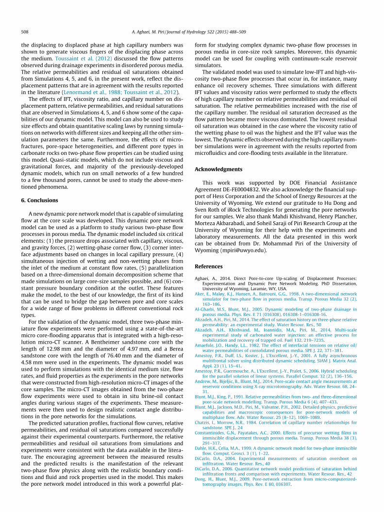
508 A. Aghaei, M. Piri / Journal of Hydrology 522 (2015) 488–509
the displacing to displaced phase at high capillary numbers wasshown to generate viscous fingers of the displacing phase acrossthe medium. Toussaint et al. (2012) discussed the flow patternsobserved during drainage experiments in disordered porous media.The relative permeabilities and residual oil saturations obtainedfrom Simulations 4, 5, and 6, in the present work, reflect the dis-placement patterns that are in agreement with the results reportedin the literature (Lenormand et al., 1988; Toussaint et al., 2012).
The effects of IFT, viscosity ratio, and capillary number on dis-placement pattern, relative permeabilities, and residual saturationsthat are observed in Simulations 4, 5, and 6 show some of the capa-bilities of our dynamic model. This model can also be used to studysize effects and obtain quantitative scaling laws by running simula-tions on networks with different sizes and keeping all the other sim-ulation parameters the same. Furthermore, the effects of micro-fractures, pore-space heterogeneities, and different pore types incarbonate rocks on two-phase flow properties can be studied usingthis model. Quasi-static models, which do not include viscous andgravitational forces, and majority of the previously-developeddynamic models, which run on small networks of a few hundredto a few thousand pores, cannot be used to study the above-men-tioned phenomena.
6. Conclusions
A new dynamic pore network model that is capable of simulatingflow at the core scale was developed. This dynamic pore networkmodel can be used as a platform to study various two-phase flowprocesses in porous media. The dynamic model included six criticalelements: (1) the pressure drops associated with capillary, viscous,and gravity forces, (2) wetting-phase corner flow, (3) corner inter-face adjustments based on changes in local capillary pressure, (4)simultaneous injection of wetting and non-wetting phases fromthe inlet of the medium at constant flow rates, (5) parallelizationbased on a three-dimensional domain decomposition scheme thatmade simulations on large core-size samples possible, and (6) con-stant pressure boundary condition at the outlet. These featuresmake the model, to the best of our knowledge, the first of its kindthat can be used to bridge the gap between pore and core scalesfor a wide range of flow problems in different conventional rocktypes.
For the validation of the dynamic model, three two-phase min-iature flow experiments were performed using a state-of-the-artmicro core-flooding apparatus that is integrated with a high-reso-lution micro-CT scanner. A Bentheimer sandstone core with thelength of 12.98 mm and the diameter of 4.97 mm, and a Bereasandstone core with the length of 76.40 mm and the diameter of4.58 mm were used in the experiments. The dynamic model wasused to perform simulations with the identical medium size, flowrates, and fluid properties as the experiments in the pore networksthat were constructed from high-resolution micro-CT images of thecore samples. The micro-CT images obtained from the two-phaseflow experiments were used to obtain in situ brine-oil contactangles during various stages of the experiments. These measure-ments were then used to design realistic contact angle distribu-tions in the pore networks for the simulations.
The predicted saturation profiles, fractional flow curves, relativepermeabilities, and residual oil saturations compared successfullyagainst their experimental counterparts. Furthermore, the relativepermeabilities and residual oil saturations from simulations andexperiments were consistent with the data available in the litera-ture. The encouraging agreement between the measured resultsand the predicted results is the manifestation of the relevanttwo-phase flow physics along with the realistic boundary condi-tions and fluid and rock properties used in the model. This makesthe pore network model introduced in this work a powerful plat-
form for studying complex dynamic two-phase flow processes inporous media in core-size rock samples. Moreover, this dynamicmodel can be used for coupling with continuum-scale reservoirsimulators.
The validated model was used to simulate low-IFT and high-vis-cosity two-phase flow processes that occur in, for instance, manyenhance oil recovery schemes. Three simulations with differentIFT values and viscosity ratios were performed to study the effectsof high capillary number on relative permeabilities and residual oilsaturation. The relative permeabilities increased with the rise ofthe capillary number. The residual oil saturation decreased as theflow pattern became more viscous dominated. The lowest residualoil saturation was obtained in the case where the viscosity ratio ofthe wetting phase to oil was the highest and the IFT value was thelowest. The dynamic effects observed during the high capillary num-ber simulations were in agreement with the results reported frommicrofluidics and core-flooding tests available in the literature.
Acknowledgments
This work was supported by DOE Financial AssistanceAgreement DE-FE0004832. We also acknowledge the financial sup-port of Hess Corporation and the School of Energy Resources at theUniversity of Wyoming. We extend our gratitude to Hu Dong andSven Roth of iRock Technologies for generating the pore networksfor our samples. We also thank Mahdi Khishvand, Henry Plancher,Morteza Akbarabadi, and Soheil Saraji of Piri Research Group at theUniversity of Wyoming for their help with the experiments andlaboratory measurements. All the data presented in this workcan be obtained from Dr. Mohammad Piri of the University ofWyoming ([email protected]).
References
Aghaei, A., 2014. Direct Pore-to-core Up-scaling of Displacement Processes:Experimentation and Dynamic Pore Network Modeling. PhD Dissertation,University of Wyoming, Laramie, WY, USA.
Aker, E., Maløy, K.J., Hansen, A., Batrouni, G.G., 1998. A two-dimensional networksimulator for two-phase flow in porous media. Transp. Porous Media 32 (2),163–186.
Al-Gharbi, M.S., Blunt, M.J., 2005. Dynamic modeling of two-phase drainage inporous media. Phys. Rev. E 71 (016308), 016308-1–016308-16.
Alizadeh, A.H., Piri, M., 2014. The effect of saturation history on three-phase relativepermeability: an experimental study. Water Resour. Res., 50
Alizadeh, A.H., Khishvand, M., Ioannidis, M.A., Piri, M., 2014. Multi-scaleexperimental study of carbonated water injection: an effective process formobilization and recovery of trapped oil. Fuel 132, 219–7235.
Amaefule, J.O., Handy, L.L., 1982. The effect of interfacial tensions on relative oil/water permeabilities of consolidated porous media. SPE J. 22, 371–381.
Amestoy, P.R., Duff, I.S., Koster, J., L’Excellent, J.-Y., 2001. A fully asynchronousmultifrontal solver using distributed dynamic scheduling. SIAM J. Matrix Anal.Appl. 23 (1), 15–41.
Amestoy, P.R., Guermouche, A., L’Excellent, J.-Y., Pralet, S., 2006. Hybrid schedulingfor the parallel solution of linear systems. Parallel Comput. 32 (2), 136–156.
Andrew, M., Bijeljic, B., Blunt, M.J., 2014. Pore-scale contact angle measurements atreservoir conditions using X-ray microtomography. Adv. Water Resour. 68, 24–31.
Blunt, M.J., King, P., 1991. Relative permeabilities from two- and three-dimensionalpore-scale network modelling. Transp. Porous Media 6 (4), 407–433.
Blunt, M.J., Jackson, M.D., Piri, M., Valvatne, P.H., 2002. Detailed physics, predictivecapabilities and macroscopic consequences for pore-network models ofmultiphase flow. Adv. Water Resour. 25 (8–12), 1069–1089.
Chatzis, I., Morrow, N.R., 1984. Correlation of capillary number relationships forsandstone. SPE J., 24
Constantinides, G.N., Payatakes, A.C., 2000. Effects of precursor wetting films inimmiscible displacement through porous media. Transp. Porous Media 38 (3),291–317.
Dahle, H.K., Celia, M.A., 1999. A dynamic network model for two-phase immiscibleflow. Comput. Geosci. 3 (1), 1–22.
DiCarlo, D.A., 2004. Experimental measurements of saturation overshoot oninfiltration. Water Resour. Res., 40
DiCarlo, D.A., 2006. Quantitative network model predictions of saturation behindinfiltration fronts and comparison with experiments. Water Resour. Res., 42
Dong, H., Blunt, M.J., 2009. Pore-network extraction from micro-computerized-tomography images. Phys. Rev. E 80, 036307.
A. Aghaei, M. Piri / Journal of Hydrology 522 (2015) 488–509 509
Dullien, F.A.L., 1992. Porous Media: Fluid Transport and Pore Structure, second ed.Academic Press, San Diego.
du Prey, E.J.L., 1973. Factors affecting liquid–liquid relative permeabilities of aconsolidated porous medium. SPE J. 13, 39–47.
Fatt, I., 1956a. The network model of porous media I. Capillary pressurecharacteristics. Trans. Am. Inst. Min., Metall., Petrol. Eng. 207, 144–159.
Fatt, I., 1956b. The network model of porous media II. Dynamic properties of asingle size tube network. Trans. Am. Inst. Min., Metall., Petrol. Eng. 207, 160–163.
Fatt, I., 1956c. The network model of porous media III. Dynamic properties ofnetworks with tube radius distribution. Trans. Am. Inst. Min., Metall., Petrol.Eng. 207, 164–181.
Fourie, W., Said, R., Young, P., Barnes, D., 2007. The simulation of pore scale fluidflow with real world geometries obtained from X-ray computed tomography.In: Proceedings of the COMSOL Conference, Boston.
Gabriel, E., Fagg, G.E., Bosilca, G., Angskun, T., Dongarra, J.J., Squyres, J.M., Sahay, V.,Kambadur, P., Barrett, B., Lumsdaine, A., Castain, R.H., Daniel, D.J., Graham, R.L.,Woodall, T.S., September 2004. Open MPI: goals, concept, and design of a nextgeneration MPI implementation. In: Proceedings, 11th European PVM/MPIUsers’ Group Meeting. Budapest, Hungary, pp. 97–104.
Gingold, R., Monaghan, J., 1997. Smoothed particle hydrodynamics: theory andapplication to non-spherical stars. Mon. Notices Roy. Astron. Soc. 181, 375–7389.
Green, D.W., Willhite, G.P., 1998. Enhanced Oil Recovery, first ed. SPE, Richardson,TX.
Hashemi, M., Sahimi, M., Dabir, B., 1998. Percolation with two invaders and twodefenders: volatile clusters, oscillations, and scaling. Phys. Rev. Lett. 80, 3248.
Hashemi, M., Dabir, B., Sahimi, M., 1999a. Dynamics of two-phase flow in porousmedia: simultaneous invasion of two fluids. AIChE J. 45, 1365.
Hashemi, M., Sahimi, M., Dabir, B., 1999b. Monte Carlo simulation of two-phaseflow in porous media: Invasion with two invaders and two defenders. Physica A267, 1.
Hassanizadeh, S.M., Gray, W.G., 1990. Mechanics and thermodynamics ofmultiphase flow in porous media including interphase boundaries. Adv.Water Resour. 13, 169–186.
Hughes, R.G., Blunt, M.J., 2000. Pore scale modeling of rate effects in imbibition.Transp. Porous Media 40 (3), 295–322.
Hui, M.H., Blunt, M.J., 2000. Effects of wettability on three-phase flow in porousmedia. J. Phys. Chem. B 104 (16), 3833–3845.
Inamuro, T., Ogata, T., Tajima, S., Konishi, N., 2004. A Lattice Boltzmann method forincompressible two-phase flows with large density differences. J. Comput. Phys.198, 628644.
Joekar-Niasar, V., Hassanizadeh, S.M., 2012. Analysis of fundamentals of two-phaseflow in porous media using dynamic pore-network models: a review. Crit. Rev.Environ. Sci. Technol. 42:18, 1895–1976.
Joekar-Niasar, V., Hassanizadeh, S.M., Dahle, H.K., 2010. Non-equilibrium effects incapillarity and interfacial area in two-phase flow: dynamic pore-networkmodelling. J. Fluid Mech., 655
Kamath, J., Xu, B., Lee, S., Yortsos, Y., 1996. Pore network modeling of laboratoryexperiments on heterogeneous carbonates. In: Paper SPE 36681, Proceedings ofthe SPE Annual Technical Conference and Exhibition, Denver, Colorado, 6–9October.
Karpyn, Z.T., Piri, M., 2007. Prediction of fluid occupancy in fractures using networkmodeling and X-ray microtomography. I: Data conditioning and modeldescription. Phys. Rev. E 76 (016315). http://dx.doi.org/10.1103/PhysRevE.76.016315.
Khishvand, M., Akbarabadi, M., Piri, M., 2015. A pore-scale experimentalinvestigation of dynamic effects and matrix dissolution in naturally-occurringporous media using X-ray microtomography. AIChE Journal. (submitted forpublication).
Knudsen, H.A., Hansen, A., 2002. Relation between pressure and fractional flow intwo-phase flow in porous media. Phys. Rev. E 65 (5).
Koplik, J., Lasseter, T., 1985. Two-phase flow in random network models of porousmedia. SPE J., 25
Koshizuka, S., Tamako, H., Oka, Y., 1995. A particle method for incompressibleviscous flow with fluid fragmentation. Comput. Fluid Dyn. J. 4 (1), 29–746.
Lake, L.W., 1989. Enhanced Oil Recovery, first ed. Prentice Hall, Englewood Cliffs,NJ.
Lee, S.H., Padmanabhan, L., Al-Sunaidi, H.A., 1995. Simulation of linear displacementexperiments on massively parallel computers. In: Paper SPE 30721, Proceedingsof the SPE Annual Technical Conference and Exhibition, Dallas, TX, 22–25October.
Lenormand, R., Touboul, E., Zarcone, C., 1988. Numerical models and experimentson immiscible displacements in porous media. J. Fluid Mech. 189 (April), 165–187.
Lerdahl, T.R., Øren, P.E., Bakke, S., 2000. A predictive network model for three-phaseflow in porous media. In: Paper SPE 59311, Proceedings of the SPE/DOESymposium in Improved Oil Recovery, Tulsa, Oklahoma, 3–5 April.
Li, H., Pan, C., Miller, C., 2005. Pore-scale investigation of viscous coupling effects fortwo-phase flow in porous media. Phys. Rev. E 72, 026705.
Løvoll, G., Méheust, Y., Måløy, K.J., Aker, E., Schmittbuhl, J., 2005. Competition ofgravity, capillary and viscous forces during drainage in a two-dimensionalporous medium, a pore scale study. Energy 30, 861–872.
Mayer, R.P., Stowe, R.A., 1965. Mercury porosimetry—breakthrough pressure forpenetration between packed spheres. J. Colloid Sci. 20, 893–911.
Mogensen, K., Stenby, E., 1998. A dynamic two-phase pore-scale model ofimbibition. Transp. Porous Media, 32.
Nguyen, V.H., Sheppard, A.P., Knackstedt, M.A., Pinczewski, W.V., 2006. The effect ofdisplacement rate on imbibition relative permeability and residual saturation. J.Petrol. Sci. Eng., 52
Nordhaug, H.F., Celia, M., Dahle, H.K., 2003. A pore network model for calculation ofinterfacial velocities. Adv. Water Resour. 26 (10), 1061–1074.
Oak, M.J., 1990. Three-phase relative permeability of water-wet Berea. In: Paper SPE20183, Proceedings of the SPE/DOE Seventh Symposium on Enhanced OilRecovery, Tulsa, Oklahoma, 22–25 April.
Øren, P.E., Bakke, S., 2003. Reconstruction of Berea sandstone and pore-scalemodelling of wettability effects. J. Petrol. Sci. Eng. 39, 177–199.
Øren, P.E., Bakke, S., Arntzen, O.J., 1998. Extending predictive capabilities to networkmodels. SPE J. 3 (4), 324–336.
Ovaysi, S., Piri, M., 2010. Direct pore-level modeling of incompressible fluid flow inporous media. J. Comput. Phys. 229, 7456–7476.
Ovaysi, S., Piri, M., 2011. Pore-scale modeling of dispersion in disordered porousmedia. J. Contam. Hydrol. 124, 68–81.
Patzek, T.W., 2001. Verification of a complete pore network simulator of drainageand imbibition. SPE J. 6 (2), 144–156.
Patzek, T.W., Silin, D.B., 2001. Shape factor and hydraulic conductance innoncircular capillaries. I. One-phase creeping flow. J. Colloid Interface Sci. 236(2), 295–304.
Piri, M., Blunt, M.J., 2005a. Three-dimensional mixed-wet random pore-scalenetwork modeling of two- and three-phase flow in porous media. I. Modeldescription. Phys. Rev. E 71 (026301). http://dx.doi.org/10.1103/PhysRevE.71.026301.
Piri, M., Blunt, M.J., 2005b. Three-dimensional mixed-wet random pore-scalenetwork modeling of two- and three-phase flow in porous media. II. Results.Phys. Rev. E 71 (026302). http://dx.doi.org/10.1103/PhysRevE.71.026302.
Piri, M., Karpyn, Z.T., 2007. Prediction of fluid occupancy in fractures using networkmodeling and X-ray microtomography. II: Results. Phys. Rev. E 76 (016316).http://dx.doi.org/10.1103/PhysRevE.76.016316.
Premoze, S., Tasdizen, T., Bigler, J., Lefohn, A., Whitaker, R., 2003. Particle-basedsimulation of fluids. Comput. Graph. Forum 22, 3.
Princen, H.M., 1969a. Capillary phenomena in assemblies of parallel cylinders I.Capillary rise between two cylinders. J. Colloid Interface Sci. 30 (1), 69–75.
Princen, H.M., 1969b. Capillary phenomena in assemblies of parallel cylinders II.Capillary rise in systems with more than two cylinders. J. Colloid Interface Sci.30 (3), 359–371.
Princen, H.M., 1970. Capillary phenomena in assemblies of parallel cylinders III.Liquid columns between horizontal parallel cylinders. J. Colloid Interface Sci. 34(2), 171–184.
Sahimi, M., 2010. Flow and Transport in Porous Media and Fractured Rock, seconded. Wiley-VCH, Los Angeles.
Saraji, S., Goual, L., Piri, M., 2013. Wettability of sc-CO2/water/Quartz systems:simultaneous measurement of contact angle and interfacial tension at reservoirconditions. Langmuir 29, 6856–6866.
Schaefer, C.E., DiCarlo, D.A., Blunt, M.J., 2000. Experimental measurement of air-water interfacial area during gravity drainage and secondary imbibition inporous media. Water Resour. Res. 36 (4), 885–890.
Sheng, Q., Thompson, K., 2013. Dynamic coupling of pore-scale and reservoir-scalemodels for multiphase flow. Water Resour. Res., 49
Singh, M., Mohanty, K.K., 2003. Dynamic modeling of drainage through three-dimensional porous material. Chem. Eng. Sci. 58, 1–18.
Stauffer, F., 1978. Time dependence of the relations between capillary pressure,water content and conductivity during drainage of porous media. In: IAHRSymposium on Scale Effects in Porous Media, Thessaloniki, Greece, pp. 3.35–3.52.
Tartakovsky, A., Meakin, P., 2005. A smoothed particle hydrodynamics for miscibleflow in three-dimensional fractures and two-dimensional Rayleigh–Taylorinstability. J. Comput. Phys. 207, 610–7624.
Thompson, K.E., 2002. Pore-scale modeling of fluid transport in disordered fibrousmaterials. AIChE J. 48 (7).
Tørå, G., Øren, P.-E., Hansen, A., 2012. A dynamic network model for two-phase flowin porous media. Transp. Porous Media 92, 145–164.
Toussaint, R., Måløy, K.J., Méheust, Y., Løvoll, G., Jankov, M., Schäfer, G., Schmittbuhl,J., 2012. Two-phase flow: structure, upscaling, and consequences formacroscopic transport properties. Vadose Zone J. 11 (3). http://dx.doi.org/10.2136/vzj2011.0123.
Valvatne, P.H., Blunt, M.J., 2004. Predictive pore-scale modeling of two-phase flowin mixed wet media. Water Resour. Res. 40, W07406.
van der Marck, S.C., Matsuura, T., Glas, J., 1997. Viscous and capillary pressuresduring drainage: network simulations and experiments. Phys. Rev. E 56 (5),5675–5687.
Xu, B., Kamath, J., Yortsos, Y., Lee, S., 1999. Use of pore-network models to simulatelaboratory corefloods in a heterogeneous carbonate sample. SPE J. 4 (3), 179–186.
Zhu, Y., Fox, P.J., Morris, J.P., 1999. A pore-scale numerical model for flow throughporous media. Int. J. Numer. Anal. Methods Geomech. 23, 881–7904.


![References [1] Mogensen, M., Sammes, N.M. & Tompsett, G.A. (2000) Solid State Ionics 129 , 63-94.](https://static.fdocuments.us/doc/165x107/568163f5550346895dd58247/references-1-mogensen-m-sammes-nm-tompsett-ga-2000-solid-state.jpg)