Journal of Fluids and Structures - Indian Institute of...

Contents lists available at ScienceDirect

Journal of Fluids and Structures

Journal of Fluids and Structures 66 (2016) 517–542

http://d0889-97

n CorrE-m

journal homepage: www.elsevier.com/locate/jfs

Flow patterns and efficiency-power characteristics of aself-propelled, heaving rigid flat plate

Nipun Arora a, Amit Gupta a,n, Sanjeev Sanghi b, Hikaru Aono c, Wei Shyy d

a Department of Mechanical Engineering, Indian Institute of Technology, Hauz Khas, New Delhi 110016, Indiab Department of Applied Mechanics, Indian Institute of Technology, Hauz Khas, New Delhi 110016, Indiac Department of Mechanical Engineering, Tokyo University of Science, Katsushika-Ku, Tokyo 125-8585, Japand Department of Mechanical and Aerospace Engineering, Hong Kong University of Science and Technology, Hong Kong

a r t i c l e i n f o

Article history:Received 27 May 2016Received in revised form21 July 2016Accepted 25 August 2016

Keywords:Reynolds numberAmplitudeDensity ratioWing–wake interactionVortex dipolePower and efficiency

x.doi.org/10.1016/j.jfluidstructs.2016.08.00546/& 2016 Elsevier Ltd. All rights reserved.

esponding author.ail address: [email protected] (A. Gupta

a b s t r a c t

The aim of the present study is to characterize the flow patterns, propulsion efficiency andpower requirements associated with a self-propelled-heaving thin flat plate in a quiescentmedium. In this regard, a numerical model using a shifting discontinuous-grid and basedupon multi-relaxation-time lattice Boltzmann method is developed to probe the resultingaerodynamics. The influence of kinematic parameters namely flapping Reynolds numberRef (20�100) and plunging amplitude β (0.2–1), and the density ratio ρ* (101�102) onforward flight is pursued. Depending on the kinematics, various periodic vortex sheddingcharacteristics of the plunging plate are observed that lead to modification of the angle ofattack as a result of wing-wake interaction and downward jet. The presence of strongvortex dipole at the trailing edge with an attached leading edge vortex are factors re-sponsible for maximum thrust generation. A wing-wake interaction which occurs at low βand high Ref due to weak vortex dissipation and presence of vortex dipole at the trailingedge acting in tandem can lead to achieving high propulsion efficiency. Through surrogatemodelling, a set of Pareto-optimal solutions that describe the tradeoff between efficiencyand input power for forward flight is presented and offers insight into the design anddevelopment of next generation flapping wing micro-air vehicles.

& 2016 Elsevier Ltd. All rights reserved.

1. Introduction

With a dimension span of 15 cm or smaller and flight speed of �10 m/s or lower, micro-air vehicles (MAVs) operate inlow Reynolds number (Reo104) regimes and experience aerodynamic conditions with low lift-to-drag ratios (Shyy et al.,2008, 2013, 2010). These are rapidly evolving as modern defense gadgets for performing surveillance and reconnaissanceoperations with prerequisites of high-maneuverability, stable hover, vertical take-off/landing capability, swiftness andnoiseless locomotion (Shyy et al., 2008, 2013, 2010; Tsai and Fu, 2009; Muller, 2001). While alternative MAV concepts basedon fixed wing, rotary wing and flapping wing have been explored, flapping flight has carved its superiority over otherdesigns with excellent maneuverability through space, navigation and control capabilities, stimulating researchers to de-velop and design this class of MAVs, including Nano-humming bird (Keennon et al., 2012), Microrobot (Fuller et al., 2014; Maet al., 2015) and Delfly (Croon et al., 2016).

).

www.sciencedirect.com/science/journal/08899746

www.elsevier.com/locate/jfs

http://dx.doi.org/10.1016/j.jfluidstructs.2016.08.005



http://crossmark.crossref.org/dialog/?doi=10.1016/j.jfluidstructs.2016.08.005&domain=pdf



mailto:[email protected]


N. Arora et al. / Journal of Fluids and Structures 66 (2016) 517–542518

Nevertheless, as discussed by Shyy et al. (2016) and Chin and Lentink (2016), significant milestones are yet to be achievedfor establishing comprehensive predictive capabilities of flapping flight concepts towards development of MAVs capable ofcovering the wide range of flight conditions encountered in practical operation. In addition, the flight of insects and birdswhich involves complex flapping motions do not follow the classical aerodynamics based quasi-steady mechanisms of liftgeneration without taking into account of the flow characteristics surrounding the flapping wing (Shyy et al., 2009; Trizilaet al., 2011; Shyy et al., 1999; Sane, 2003; Alexander, 2002; Dickinson et al., 1999; Arora et al., 2014). Developing a betterunderstanding of this process which addresses the issues of scaling and energy optimization (Kang et al., 2011; Kang andShyy, 2013, 2014; Lee et al., 2015; Quinn et al., 2013) is expected to assist in simplified MAV design.

The phenomenon of thrust generation in birds was first reported by Knoller (1909) and Betz (1912), and hence is knownas the Knoller–Betz effect. By considering a vertically heaving airfoil as a representation of bird wings, they stated that due tothe plunging motion of wing an effective angle of attack was created which provided a force component in the horizontaldirection and was responsible for thrust production, which was later experimentally proved by Katzmayr (1922). Manyexperimental and computational studies on rigid wing performing pure plunging motion (some studies also included activepitching) were conducted which supported the above argument (Freymuth, 1988, 1990; Triantafyllou et al., 1991; Lai andPlatzer, 2000; Jones et al., 1998; Anderson et al., 1998; Lewin and Haj-Hariri, 2003). In all these studies either the wingflapped at a fixed position with an oncoming flow or the wing cruised through the flow whose speed could be controlledindependently. Taking it further, the present study is conducted on a rigid self-propelled heaving airfoil (the forwardtranslation is produced only due to flapping motion and both of them are interdependent or coupled) to mimic the op-eration of a biological flyer.

Some of the key findings of previous studies on an auto-propelled wing (Vandenberghe et al., 2004; Vandenberghe et al.,2006; Alben and Shelley, 2005; Lu and Liao, 2006; Zhang et al., 2009; Benkherouf et al., 2011; Hu and Xiao, 2014) aresummarized here. Vandenberghe et al. (2004, 2006) experimentally revealed the presence of a stability limit beyond whicha pure oscillating rectangular plate mounted on an axle can rotate in the transverse direction, indicating the onset of thegeneration of thrust. Alben and Shelley (2005), using an elliptical wing, numerically investigated the earlier (Vandenbergheet al., 2004) experiment and showed that beyond a critical Reynolds number (based on flapping frequency), unidirectionallocomotion can be achieved for an initially non-locomoting body. Lu and Liao (2006) quantified the critical Reynoldsnumber by varying the amplitude of an elliptical membrane and studied the dynamical behavior of the foil with differentdensity ratios, and classified it as (a) steady, or (b) oscillatory movement. Zhang et al. (2009) studied the effect of varying thechord-thickness ratio (CR) for an elliptical and rectangular flapping foil between 1 and 100 on the symmetry breakingbifurcation. Hu and Xiao (2014) examined the propulsive performance of a three-dimensional plunging elliptical airfoil byvarying the density and aspect ratio (defined as the span to chord ratio) and showed that the translational velocity andthrust coefficient increase with an increase in the aspect ratio.

These earlier studies demarcate the zones of stability/instability and quantify the critical plunging frequency or flappingReynolds number beyond which pure plunging motion leads to thrust generation, as a function of amplitude, density andchord-thickness ratio. Furthermore, power requirements and efficiency for propulsion of a self-propelled airfoil due tointerplay of flapping Reynolds number Ref, plunging amplitude β and wing-fluid density ratio ρ* need to be addressed. Weaim to present a quantitative assessment of such issues for the zone in which propulsion is attained, develop their reduced-order models and highlight the relative impact of the governing parameters for a thin, rigid and plunging flat plate. Hence,the following are the key objectives of this work:

1. investigate the impact of flapping Reynolds number Ref, plunging amplitude β and density ratio ρ* on the propulsionvelocity and energy requirements of a rigid-flat plate,

2. highlight the dominant flow structures that capture and explain the dynamics of thrust generation in a self-propelledplunging plate, and

3. formulate reduced-order models through surrogate modelling to establish a relationship between performance (powerand efficiency) and system parameters (Ref, ρ* and β). Thereafter, identify the optimum operating conditions in forwardflight including any tradeoff between these two performance parameters.

To the best of our knowledge, impact assessment of the chosen variables on propulsive performance of a plunging wingwith the help of reduced-order models has not been pursued so far.

2. Problem description

2.1. Plunging kinematics and parameters

We consider an auto-propelled heaving rigid flat plate, unconstrained to translate in the horizontal direction, whereasplunging takes place in the vertical direction. The following parameters which are expected to play a vital role in propulsionare introduced to conduct a parametric study on the plunging airfoil. Chord C has been chosen as the length scale andflapping duration T (where γ=T 1/ and γ is the plunging frequency) as time scale for non-dimensionalizing them.

The dimensionless vertical displacement of the flat plate is given as

N. Arora et al. / Journal of Fluids and Structures 66 (2016) 517–542 519

β π( *) = − ( *) ( )y t tcos 2 1

where γ* =t t and β = A C/ is the dimensionless plunging amplitude.The flapping Reynolds number based on frequency is defined as

γυ

= ( )A C

Re 2f

where υ is the kinematic viscosity.Due to the fluid–airfoil interaction, a hydrodynamic force is exerted on the flat plate. The horizontal component of this

force will be responsible for the forward locomotion along the x-axis. The dimensionless horizontal position of the plate *xp

is updated by the following equation

π βρ δ

*

*= * ( )

d x

dtF

23

px

2

2

2 2

In Eq. (3), Fx is the thrust coefficient defined as

ρ=

¯

( )F

F

V C 4x

x

f12

2

where π γ=V A2 is the maximum plunging velocity, Fx is the instantaneous thrust calculated using momentum exchangemethod and is explained in Section IIIA.2.

ρ* is the density ratio defined as

ρρρ

* =( )5

s

f

where ρs and ρf are the densities of the plate and fluid, respectively. δ is the thickness to chord ratio which been fixed at 2%in this work and is very close to that of a real insect wing (Shyy et al., 2008, 2010). Zhang et al. (2009) in their study showedthat for δ ≤2%, rectangular foils propelled faster than elliptic ones. Hence, all analysis has been conducted assuming arectangular cross-sectional shape of the wing.

The dimensionless velocity component in the horizontal direction U, is updated by the following rule

πβ= =

** ( )

UuV

dx

dt1

2 6p

where u is the dimensional instantaneous translational velocity. The translational Reynolds number is defined as

υ=

¯( )

u CRe 7u

where u is the time-averaged translational velocity attained by the plate at cruising condition.Another important dimensionless number related to the flapping flight indicative of the vortex shedding is the Strouhal

number which is defined as

γ=

¯ ( )StAu 8

w

where Aw is the width of the wake and is taken as 2 A (twice the plunging amplitude) (Lu and Liao, 2006). Strouhal numbercan also be expressed as =St 2Re /Ref u

and it represents the ratio of plunging acceleration forces to the pressure or thrust/drag forces generated due to flapping. In terms of time scales, it is a comparison of the time taken to horizontally traversecharacteristic length (chord C in present study) with the plunging time period (Benkherouf et al., 2011).

Table 1 shows the parameter range, type of model and shape of wing considered in the earlier studies on self-propelledrigid plunging wing along with their key contributions. Although significant findings for identification of critical parametersgoverning propulsion were reported, none of these studies covered aspects related to flow patterns and the collectiveimpact of these parameters on efficiency and input power at cruising conditions. Moreover, these analyses have inherentlyemployed thick plates or elliptical membranes, and a density ratio that may not be compatible with the morphologicalparameters of biological flyers.

To obtain an exhaustive understanding of the dynamics associated with the parameters of interest, the selection of therange of design variables encompassing these earlier studies was deemed necessary. Hence, a range of parameters which isalso in agreement with that of smallest insect flight (such as Encarsia Formosa and Drosophila melanogaster) (Shyy et al.,2008, 2010) and as shown in Table 2 has been chosen. Moreover, it has earlier been shown that for low ρ*, high β and

≤Re 10f , an instability leading to translation does not result in a steady propulsive velocity (Alben and Shelley, 2005). Sincethe focus of this work is on efficiency and power quantification for steady flight (or cruising condition), thus, the lower limitfor Ref was chosen to be Ref¼20. It should also be noted that the wing or tail of flying and swimming animals has a density

Table 2The range of parameters (or design space) considered in this work for surrogate modelling.

Design Variable Minimum value Maximum value

ρ* 10 100Ref 20 100β 0.2 1

Table 1Highlights of earlier studies on self-propelled rigid plunging membrane.

Reference Model/Shape Parameter Range Merits

Alben and Shelley (2005) 2-D numerical, Elliptical membrane β ¼ 0.5 (a) First simulation of a rigid self-propelledwingδ ¼ 5–30.3%

(b) Determined critical Re as a function of ρ*ρ*¼1–100Ref ¼ 1–50

Vandenberghe et al. (2004),Vandenberghe et al. (2006)

Experimental Flat plate β ¼ 0.2–0.65 (a) Originated the novel idea of a self-pro-pelled wingδ ¼ 8.4�16.8%

ρ* ¼ 7.2Ref ¼ 1–1500

Lu and Liao (2006) 2-D numerical Elliptical membrane β ¼ 0.2–1 (a) Determined critical Re as a function of βδ ¼8.3%ρ*¼ 1–100Ref ¼ 1–100

Zhang et al. (2009) 2-D numerical Flat plate & Ellipticalmembrane

β ¼ 0.4 (a) First study to consider wing shape andthickness effectsδ ¼ 1–100%

ρ* ¼ 4 (b) Determined critical Re as a function of δRef ¼ 31.84

Hu and Xiao (2014) 3-D numerical Elliptical membrane β ¼ 0.5 (a) First study to consider three-dimen-sional effectsδ ¼ 10%

ρ* ¼ 4–32Ref ¼ 20�80


ratio ρ*~ −10 101 3 (Lu and Liao, 2006). In this work ρ* has been considered to lie within −10 101 2 in order to avoid issuesrelated to convergence of numerical solution in larger density ratio scenarios.

The cycle-averaged input power *Pi is given as

∫* = ( )+

PT

F v dt1

9it

t T

y

Here Fy is the instantaneous vertical force acting on the plunging wing and T is the time duration of one cycle. For thesake of comparison, the input power can be non-dimensionalized to obtain the power coefficient Pi as

ρ=

*

( )P

P

V C 10i

i

f12

3

In self-propelled studies, the net horizontal force is zero at the cruising condition (thrust balances the drag) and hence,the output power cannot be calculated in a fashion similar to the input power (Schultz and Webb, 2002). Instead of power,the averaged kinetic energy per cycle due to forward motion, which represents the output work, is calculated (Kern andKoumoutsakos, 2006) and is given by

∫= ( )+

ET

mu dt1 1

2 11t

t T2

The propulsive efficiency η is a measure of the performance of the forward locomotion obtained by the plunging plateand is calculated as

η = ( )E

W 12

where W is the input work per cycle given by


= * ( )W P T. 13i

3. Methodology

The present study encompasses two stages of numerical modelling: (a) Fluid solver, for deciphering the fluid flow aroundplunging wing and force calculation due to fluid-structure interaction, and (b) Surrogate modelling, for formulating a re-lationship between the objective functions (i.e. efficiency and power) and design parameters (i.e. Ref, ρ* and β). The de-scription of these approaches is given in the following sections.

3.1. Fluid solver

The lattice Boltzmann method (LBM) which involves the solution of discretized Boltzmann equation for the particledistribution function (Ladd, 1994; Succi, 2001; Chen and Doolen, 1998), has been used for performing the numerical si-mulations. The most popular amongst the LB methods is the Bhatnagar, Gross and Krook (BGK) or the single-relaxation-time(SRT) model. However, SRT exhibits numerical instability at high Re (low values of relaxation time) and displays spuriousoscillations in force measurement (Arora et al., 2016). Sighting these disadvantages which posed an impediment in solvingthe fluid flow, the authors moved on to the multi-relaxation-time (MRT) model that successfully overcame the problemsfaced and has thus been employed in the present study. A brief description of this method in given in the Appendix andcalculation of macroscopic variables (flow field around the wing, i.e. u, v and p) from the distribution functions is providedin our earlier publication (Arora et al., 2014). The moving boundary condition and force calculation are reiterated here.

3.1.1. Treatment of moving boundaryFor the case of a moving boundary, the solid surface is represented by a set of boundary nodes which lie at the mid points

of the links connecting the fluid and solid nodes. With reference to Fig. 5 in Arora et al. (2014), the distribution functionsreflected back from the solid into the fluid nodes can be written as

ρ( + ) = ( ) +( )α α α α¯ ¯f t f t w

cx x e u, 1 , 2

3.

14f s b2

The last term in Eq. (14) accounts for the momentum transfer between the fluid and moving solid boundary (Ladd, 1994).Here = −α α¯e e and ub is the velocity of the boundary node, assumed to be located exactly halfway along the link betweensolid and fluid nodes, and is given by

ω= + × + −( )α

⎛⎝⎜

⎞⎠⎟u U x e X

12 15b

where U is the translational velocity, ω is the angular velocity and X is the position vector of the center of mass of the solid.In this method, the lattice nodes on either side of the boundary surface are treated in an identical fashion, i.e., the fluid

fills the entire domain (Ladd, 1994). With this modification, at each boundary node the two incoming distributions ˜ ( )αf tx,and ˜ ( + )α α¯f tx e , from the fluid and the solid sides, respectively, corresponding to velocities αe and αe along the link con-necting x and + αx e , are updated according to,

ρ( + + ) = ˜ ( + ) +( )α α α α α α¯f t f t w

cx e x e e u, 1 , 2

3.

16b2

ρ( + ) = ˜ ( ) −( )α α α α¯f t f t w

cx x e u, 1 , 2

3.

17b2

This approach ensures that mass is conserved at the boundary nodes and also avoids the necessity of creating anddestroying fluid as the solid particle moves (covering/uncovering of the fluid/solid nodes).

3.1.2. Force calculationDue to the boundary node interactions, a force is exerted on the solid which is given by

ρ+ + = ˜ ( ) − ˜ ( + ) −( )α α α α α α α¯

⎛⎝⎜

⎞⎠⎟

⎡⎣⎢

⎤⎦⎥t f t f t w

cF x e x x e e u e

12

,12

2 , , 23

.18b2

The total force F on the solid object is obtained by summing F over all the nodes that constitute the boundary of theobject along the directions α which involve the exchange of distributions from fluid to solid nodes or vice-versa,

∑ ∑¯ + = + +( )α

α⎛⎝⎜

⎞⎠⎟

⎛⎝⎜

⎞⎠⎟t tF F x e

12

12

,12 19all xb

The overall force is calculated at the intermediate integer time step by taking the average of the total forces at half integer


time steps,

( )¯ = ¯ − + ¯ +( )

⎡⎣⎢

⎛⎝⎜

⎞⎠⎟

⎛⎝⎜

⎞⎠⎟⎤⎦⎥t t tF F F

12

12

12 20

Issues pertaining to the accuracy of force measurement can be resolved by improving the resolution of the moving bodyby refining the mesh near the surface of the solid to capture the minutest of details. However, refinement of the gridthroughout the domain (even in those regions where the flow is not expected to evolve rapidly) is computationally ex-pensive and inefficient. Thus, the present study employs a novel and an unconventional shifting discontinuous-grid-blockLBM where a fine block translates with the moving solid on a carpet of coarse block (Arora et al., 2016). In this method, thefine block shifts by Δm xf (where Δ Δ=m x x/c f is the grid refinement ratio and Δxf is the lattice spacing in fine block) alongthe X or Y direction as the solid (wing) traverses a unit lattice in coarse block i.e. Δxc. Hence, at the end of a unit time step incoarse grid, the distance propagated by the object in fine grid is examined. If it exceedsΔxc, a layer of fine grid is added(removed) along (against) the direction of translation.

3.1.3. Computational domainA pictorial representation of the computational domain is shown in Fig. 1. As shown, a dynamic multi-block (finer mesh) has

been considered around the structure in an overall domain of size 50C�20C in coarse lattice units. The leading edge of wing waspositioned 20C downstream of the inlet and 30C upstream of the outlet. No slip boundary condition (zero fluid velocity) wasapplied on the top and bottomwalls of the domain along with the inlet. At the outlet, fully developed boundary condition (zeronormal derivative of velocity i.e. ∂ ∂ =u x/ 0) was imposed. Similar to the fine-block, the entire computational domain shifted withthe movement of the wing. Therefore, as the wing translated a unit distance in the coarse block, a layer of fluid nodes wasremoved from outlet and added at the inlet. When adding new layers, the post collision distribution functions at the existinginlet boundary were replicated onto the newly added layer. This ensured that far upstream the pressure gradient was zero i.e.∂ ∂ =p x/ 0. Hence, with this technique a finite domain can be epitomized as an infinite region.

To benefit from the use of LBM, the code developed was parallelized using MPI (Message Passing Interface) in which thedomain along the x direction is sliced into n sub-zones, where n is the number of processors. Thus, each processor isassigned a sub-domain with (50/n)C x 20C physical size.

3.1.4. Convergence and validationTo test for the mesh independence and convergence of the numerical method, three cases with progressively improved

mesh resolutions were examined. In case 1, a uniform coarse grid without any local refinement was considered. Whereas in

Fig. 1. Layout of the computational domain with imposed boundary conditions segregated into different zones (by red lines) handled by multi-processors.A recently developed discontinuous-grid-block LBM is implemented where a fine block translates with the moving solid on a carpet of coarse block (Aroraet al., 2016).(For interpretation of the references to color in this figure,the reader is referred to the web version of this article.)

Table 3Mesh resolution for different cases shown in Fig. 3.

Description Grid Spacing

Uniform coarse grid Case 1 Δ =x C0.01

Uniform coarse grid with local refinement (moving fine block) Case 2 Δ Δ= =x C x C0.005 , 0.01f c

Case 3 Δ Δ= =x C x C0.0025 , 0.005f c


case 2 and case 3, a fine mesh was taken around the wing (with grid refinement ratio m¼2). The description of the gridspacing for these cases is given in Table 3. The dimensions of the dynamic fine mesh block which moved along with thewing was taken as 2C�3C to ensure that the plunging plate was well confined within the boundaries of the fine block. Theconvergence test for the size of moving mesh was also performed and it was observed that the horizontal velocity profilewith the current dimensions of moving fine mesh exhibited good agreement with the stationary fine mesh that spanned theentire horizontal length of the computational domain (i.e., 50C�3C).

Fig. 2 shows a schematic diagram of the orientation of the thrust and drag force associated with the vertical plungingmotion considered in this study. Since drag always opposes the imposed motion, it acts along the vertical direction and thethrust (analogous to lift) responsible for propulsion acts horizontally.

A comparison of the dimensionless thrust < >Fx and drag < >Fy with time between these cases is shown in Fig. 3. Asevident, there is not much deviation in the forces and the degree of quantitative agreement with case 3 improves from case1 to case 2. However, to strike a balance between accuracy associated with mesh resolution and computational expenses,grid parameters corresponding to case 2 were chosen for performing all numerical simulations.

A moving average method, that resulted in change in average force coefficients by o10�3%, has been used to reducefluctuations and smoothen the force history over the entire simulation period (Arora et al., 2014). One of the reasons thatdirectly contributes to these fluctuations was the fact that in halfway bounceback LBM, certain grid points undergo tran-sitions from non-fluid region to fluid region or vice versa due to movement of the solid. Thus, the number of fluid nodes isnot conserved and the volume occupied by the solid object varies which contributes to the noise. A few earlier studies havealso reported such oscillations in their force measurements pertaining to the moving boundary using LBM (Arora et al., 2016,Aono et al., 2010; Lallemand and Luo, 2003.).

In order to validate the solver, simulations for a symmetric elliptical airfoil at different flapping Reynolds numbers wereconducted and the corresponding translational Reynolds number Reu was compared against the numerical results of Alben

Fig. 2. A schematic representation of the plunging wing with direction of thrust and drag forces.

Fig. 3. A comparison in (a) thrust and (b) drag coefficients with different grid spacing at Ref ¼ 20, β ¼ 0.4 and ρ* ¼ 55. The description of mesh resolutionfor these cases is given in Table 3. The inset shows zoomed version of rectangular snapshot.

Fig. 4. A comparison of translational Reynolds number Reu as a function of flapping Reynolds number Ref between present study and Alben and Shelley(2005) for an elliptical airfoil with ρ* ¼ 32, β ¼ 0.5 and δ ¼ 0.1.


and Shelley (2005). The ratio of amplitude to chord β and mass density ratio ρ* was taken as 0.5 and 32, respectively as wasconsidered in their work (Alben and Shelley, 2005). The thickness to chord of the elliptical membrane, δ , was kept constantas 0.1. The translational Reynolds number Reu in the present study was calculated by time-averaging the horizontal velocityover 10 plunging cycles after forward flight was achieved. As is shown in Fig. 4, the results obtained show good qualitativeand quantitative agreement and were used to validate the numerical model.

3.2. Surrogate modelling

Surrogate modelling involves construction of a continuous function (or surrogate) of a set of independent ‘design’variables from a limited amount of data that could have been obtained from pre-computed high fidelity simulations orphysical measurements. It helps in systematically organizing data to ascertain the interplay between different variables. Thisreduced-order model also offers a global outlook and assists in determining the influence on the dependent variables whichotherwise may not be ascertainable by individually varying each design variable. The surrogates provide fast evaluations ofthe various modelling and design scenarios, thereby making sensitivity and optimization studies feasible (Quiepo et al.,2005; Goel et al., 2008; Shyy et al., 2001; Shyy et al., 2011).

3.2.1. Design spaceSurrogate modelling begins by identifying the range (minimum and maximum values) in which the ‘design’ or in-

dependent variables are to be studied. This process is known as setting up of the design space. Thereafter, a number oflocations in this design space are chosen systematically where numerical simulations or physical experiments will beconducted. The set of locations comprise what is known as the Design of Experiments (DOE). The two commonly usedprocedures for the creation of DOE are Face Centred Cubic Design (FCCD) and Latin Hypercubic Sampling (LHS). FCCDprovides a total of 2Nþ2Nþ1 sampling points in a normalized design space: 2N corner points, 2N face-centred points and1 body-centred point (Goel et al., 2008), where N is the number of design variables. LHS generates sampling points bymaximizing the minimum distance between them and is usually employed after FCCD to obtain additional test points or tofill in the remainder of design space.

3.2.2. Surrogate modelsOnce data is obtained at the selected ‘training’ points of DOE, it is used for framing the surrogate model and carrying out a

sensitivity analysis. Surrogate models can be categorized in two groups, namely parametric (e.g., Polynomial Response Surface(PRS), Kriging) and non-parametric (e.g., Neural Networks) (Quiepo et al., 2005). The surrogates constructed in this study arebased on the PRS and Kriging approach. In polynomial response surface, the function of interest g is approximated as a linearcombination of polynomial functions of design variables y (Quiepo et al., 2005; Goel et al., 2008; Shyy et al., 2001).

∑ ε( ) = ( ) +( )

g h ay y21i

i i

Here hi is estimated through a least-squares method so as to minimize the variance, ( )a yi are basis functions, i is the


number of terms which depend on the degree of PRS chosen and the errors ε have an expected value (i.e., ε ) equal to zero.The adjusted coefficient of multiple determination (Radj

2) computes the prediction capability of the polynomial responsesurface approximation (Shyy et al., 2011) which is defined as

σ= −

( − )∑ ( − ¯ ) ( )=

RN

y y1

1

22adj

a s

iN

i

22

12s

where Ns is the number of sample or training points, yi is the true or actual value of the objective function, σa is the RMSerror of the polynomial fit at the training points and y is the mean value of the objective function. A good polynomial fitshould have an Radj

2 value close to 1.Another parameter called as ‘Prediction Error Sum of Squares’ (PRESS) is very commonly used as a measure of the

accuracy of the constructed surrogate model and quantifying the error (Quiepo et al., 2005; Goel et al., 2008). The root meansquare PRESS is calculated as

∑= − ^( )=

(− )⎜ ⎟⎛⎝

⎞⎠PRESS

Ny y

1

23RMS

s i

N

i i

i

1

2s

where yi is the true value at sample point x(i) and ^(− )yi

iis the estimated value using a surrogate model constructed by

considering all the sample points except the source point (x(i),yi), also known as the ‘leave-one-out’ strategy.The Kriging model estimates the objective function g as a sum of two terms: (a) linear polynomial expression and

(b) systematic departure Z (Quiepo et al., 2005; Goel et al., 2008).

∑( ) = ( ) + ( )( )

g y h a y Z y24j

j j

Z(y) symbolizes frequency variations around the model which is correlated on the basis of distance between the samplingpoints. The most popular correlation methods for evaluation of Z(y) are Gaussian, linear, exponential, cubic and spline functions.

3.2.3. Sensitivity analysisUsing the constructed surrogate model, sensitivity analysis can be performed to examine the influence of design

parameters and can be useful in assessing their hierarchical order of importance on the overall objective function (Goelet al., 2008). It also helps in measuring the extent of cross-interaction and interlinked influence of the design variableson the objective function. In the present study, a method based on the contribution of the design variables to thevariance of the objective function has been implemented (Quiepo et al., 2005). There are two sensitivity indices,namely (a) main, and (b) total sensitivity. The former is a measure of the effect of individual parameters on the changein output, whereas the latter indicates the combined or collective impact of the design variables in the outputvariation.

4. Results and discussion

In this section, results obtained for various Ref, ρ* and β through numerical simulation of a plunging thin two-dimen-sional rectangular flat plate which can freely propel in a quiescent fluid will be presented and discussed. To induce in-stability, an initial momentum corresponding to 1% of the maximum plunging velocity (in the -X-direction) was imparted tothe flat plate for the first half plunging cycle in all cases. Here instability is defined as the state when a small perturbation (inour case, a small momentum) grows causing the plunging wing (unconstrained horizontally) to propel in the direction ofimparted momentum. However, the magnitude of the small momentumwas found to not affect the final velocity at cruisingcondition other than to ensure that the wing moved towards the domain inlet (or towards left).

4.1. Hovering

While the main focus of this work is on propulsion during forward flight, it is of interest to examine a hovering scenariowhen no propulsive force is generated. As shown in Fig. 5, we consider a case for Ref¼1, ρ*¼55 and β¼0.6 in which nopropulsion was obtained. The simulation was run till 50 plunging cycles were completed with no instability being regis-tered, i.e., no horizontal locomotion was achieved and the wing only heaved up and down about a fixed mean position. InFig. 5(a), the upstroke begins, vortices form at both the edges and grow till the midstroke (shown in Fig. 5(b)). As the wingreaches the upper extreme position and starts the downstroke, both leading and trailing edge vortices are dissipated andnew opposite pair of vortices are formed (Fig. 5(c)). The vortices experience relatively large viscous dissipation by the end ofthe stroke without being shed. As a result, there is no wing-wake interaction and consequently asymmetry which couldhave driven the wing into forward motion is not realized. A similar formation and dissipation of vortices occurred during thedownstroke with the initial perturbation in the form of a small momentum failed to grow even after the plate completed theaforementioned plunging strokes.

Fig. 5. The non-dimensionalized vorticity contours used to illustrate the flow field around a flat plate at cruising condition plunging at Ref¼1 with ρ*¼55and β¼0.6. Vorticity scale chosen for non-dimensionalization is ω πβγ= 2c . The corresponding right image shows the instantaneous positions and thetrajectory during one cycle. Red and blue colors indicate anti-clockwise (out of the plane of pater) and clockwise rotation (into the plane of paper),respectively. An animation depicting the vortex evolution is provided as supplementary material (Movie 1).(For interpretation of the references to color inthis figure,the reader is referred to the web version of this article.)


Supplementary material related to this article can be found online at http://dx.doi.org/10.1016/j.jfluidstructs.2016.08.005.

4.2. Forward flight

By examining the vorticity flow structures, we describe the dynamics that emanates from the plunging motion thatimparts a forward thrust and pushes the wing into cruising condition.

The temporal variation of the dimensionless horizontal velocity of the wing for Ref¼55, ρ*¼55 and β¼0.4 is shown inFig. 6. The points (i), (ii), (iii) and (iv) marked in this figure represent the time instants t/T ¼ 0.5, 5.5, 10 and 40.5, re-spectively, at which the vorticity contours around the plate are plotted in the inset. As is evident, instability is achieved withthe initial perturbation growing in the first few plunging cycles and the wing begins to propel towards the left. Subse-quently, the velocity magnitude increases until it reaches the cruising condition at around the 20th cycle. Examination of thevorticity structures around the flat plate reveals negligibly small horizontal velocity in the early stages (i.e., (i)) as thevortical flow structures around the plate are near symmetrical. At (ii), the wing is shown interacting with the previouslyshed vortices which induces flow asymmetry resulting in thrust generation and initiation of propulsion. At (iii), the vortexattached to the trailing edge is seen interacting with an oppositely rotating vortex shed during the previous downstrokefrom the leading edge. This formation of a vortex dipole diminishes the strength of suction that would have existed whenvortices of either rotation are present unaccompanied, like at the leading edge where low pressure is created due to anattached solo LEV. Consequently, these high and low pressure regions assist in imparting a force to the wing essential forpropulsion. This phenomenon of wing wake interaction is, therefore, responsible for the growth of the initial momentumperturbation. At (iv), the wing is shown to have attained a cruising velocity with two opposite rotation vortices being shedper cycle, one during the upstroke and other during the downstroke. Both the half strokes are identical and mirror images ofeach other.

Fig. 6. Dimensionless horizontal velocity of the plunging airfoil at Ref ¼ 20, ρ*¼55 and β¼0.4 as a function of number of cycles with =Re 89.5u . Vorticitycontours of fluid flow at (i) t/T¼0.5, (ii) t/T¼5.5, (iii) t/T¼10 and (iv) t/T¼40.5 are plotted in the inset. Red and blue colors indicate anti-clockwise (out ofthe plane of pater) and clockwise rotation (into the plane of paper), respectively. An animation illustrating the vortex evolution is provided as supple-mentary material (Movie 2).(For interpretation of the references to color in this figure,the reader is referred to the web version of this article.)

Supplementary material related to this article can be found online at http://dx.doi.org/10.1016/j.jfluidstructs.2016.08.005.For this representative case of Ref¼20, β¼0.4 and ρ*¼55, the transient thrust and drag coefficients (i.e, < >Fx and < >Fy ),

normalized vertical velocity and normalized vertical displacement along with flow structures at cruising condition areshown in Fig. 7. The pressure distribution at the leading and trailing edges of the wing at maximum and minimum thrust



Fig. 7. Drag coefficient oFy4 and non-dimensional vertical velocity (upper portion) and Thrust coefficient oFx4 and non-dimensional vertical dis-placement (lower portion) at cruising condition for Ref¼20, β¼0.4 and ρ*¼55. The wing is moving leftwards (-X direction). Flow structures around thewing are shown at different time instants and responsible for crests and troughs in thrust coefficient. The inset in upper right corner displays the pressureat leading and trailing edge at time instants (a) and (b). Situations (a) and (b) correspond to >P PLE TE and <P PLE TE , respectively.

Fig. 8. Cycle-averaged propulsive efficiency η and input power coefficient Pi for Ref ¼55 with ρ*¼55 and β¼0.4.


coefficient is also shown in the inset. As can be observed, the pressure difference across the wing chord (i.e., Δ = −P P PLE TE)changes from positive to negative as the wing undergoes upstroke (moving from lowermost (a) to mean position (b)). Atposition (a), a new LEV (red) is beginning to develop on the lower side of the plate and the LEV (blue) that formed on theupper side during downstroke is about to merge with the nascent TEV of same rotation. At position (b), the LEV on the lowerside has grown and remains attached creating a zone of low pressure and the vortex near the trailing edge slips away,leading to <P PLE TE. At the end of the upstroke, flow structures similar to (a) were found to exist on the lower side of theplate and were again responsible for >P PLE TE. This reversal in pressure difference manifests in the form of time varyingthrust that changes from positive (deceleration) to negative (acceleration) and prevails throughout the cruising conditionand is responsible for the undulations registered in the velocity profile.


Fig. 8 shows the trend of cycle-averaged efficiency η and power coefficient Pi for the same case. In all simulations, asimilar behavior is observable where the input power initially increases when there is a sudden loss in symmetry of the flowfield and extra power is needed by the plate to overcome high drag. In addition, a thrust that is higher than that duringcruising condition is required to move the plate and is also evident from the power curve. Within a few cycles after the onsetof forward motion, the efficiency increases and reaches a maximum when cruising velocity is attained. It should be notedthat the cruising condition efficiency oη4 and input power oPi4 were determined by averaging over a time periodTss >> T after steady propulsion was achieved.

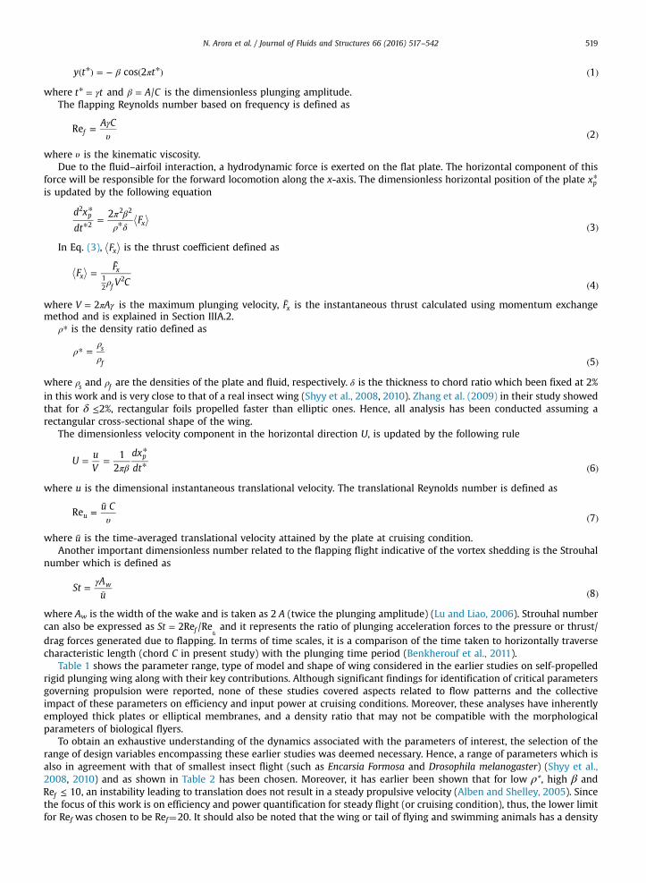
Fig. 10. Time variation of (a) drag and (b) thrust force coefficients for different Ref with β = 0.6 and ρ* = 55 at cruising conditions.

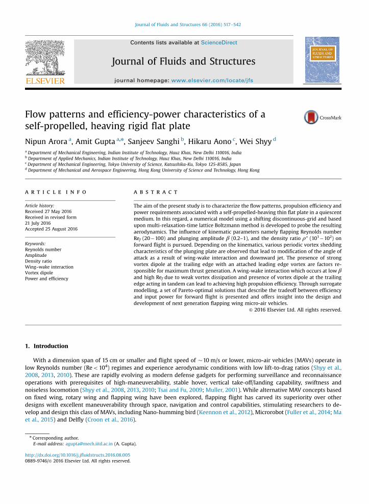
Fig. 9. Time variation of dimensionless propulsion velocity for the flat plate plunging for various Ref with ρ*¼55 and β¼0.6. The top and bottom horizontalaxis represent the time scales for Ref¼20 and 55 and Ref¼100, respectively.


4.3. Parametric analysis

We now discuss the role of plunging parameters, i.e., flapping Reynolds number Ref and plunging amplitude β, and theplate-fluid density ratio ρ* on the cruising condition and highlight their impact on power requirement oPi4 and pro-pulsion efficiency oη4 . Finally, their global implications are discussed through the developed 3rd degree polynomialresponse surfaces.

4.3.1. Effect of flapping Reynolds number (Ref)Fig. 9 shows the evolution of horizontal velocity profiles due to the action of the plunging motion for Ref¼20, 55 and 100

(with ρ*¼55 and β¼0.6). As shown in the figure, the magnitude of the non-dimensional cruising velocity at Ref¼100 ismore than double than that at Ref¼20. Due to the fact that a higher Reynolds number implies lower viscous dissipation(resulting in the likelihood of a stronger wing-wake interaction), the quantitative influence of wing-wake interaction, bothin terms of aiding or hindering, depends on the alignment of the plate with shed vortices (Arora et al., 2014) and will bediscussed shortly. More importantly, a greater number of cycles are shown to be needed to reach a cruising condition as Refincreases.

To illustrate the dependence of Ref on input power and efficiency, the time-dependent drag and thrust force coefficientsare shown in Fig. 10. From the figure it is clear that coefficients of drag and thrust for Ref¼20 show a behavior that is verydifferent from that observable for Ref¼55 and 100. In the case of the drag coefficient for Ref¼20, the variation during 38≤t/T≤38.5 (upstroke) does not mirror that during 38.5≤t/T≤39 (downstroke). As a result, the power required for driving the

Fig. 11. The time-evolution of power coefficient Pi and efficiency η for various Ref. The two parameters were calculated by averaging data at the end of eachplunging cycle. Long after the initial transient period, the two parameters can be observed to have reached stagnation values indicating attainment offorward cruising flight. Further, for plunging motion at different Ref, the input power and efficiency at cruising conditions are higher for situations withhigher Ref indicating the role of lower viscous dissipation on wing–wake interaction and reaching higher cruising velocities as shown in Fig. 9.

Fig. 12. Wake patterns at cruising condition for a flat plate plunging at Ref of (a) 20, (b) 55 and (c) 100 with ρ*¼55 and β¼0.6. The right-most columnshows the instantaneous positions during the upstroke. Red and blue colors indicate anti-clockwise (out of the plane of paper) and clockwise rotation (intothe plane of paper), respectively. (For interpretation of the references to color in this figure,the reader is referred to the web version of this article.)


heaving motion (as given by Eq. (9)) is lower for lower Ref. A similar difference in profiles is also observed for thrustcoefficient. The undulations in thrust coefficient decrease with increasing Ref which explains the decreasing fluctuations inthe horizontal velocity shown in Fig. 9. More importantly, the difference in thrust coefficient and interaction of plate withthe shed vortex renders in the form of lower efficiency for low Ref flows. To corroborate these arguments, the plunge cycle-averaged power coefficient and efficiency are plotted and shown in Fig. 11. This figure shows that long after the initialtransient period when the effects of the impulsively moving plate have passed, the two parameters approach stagnationvalues indicating attainment of forward cruising flight. Further, the input power and efficiency at cruising conditions arehigher for situations with higher Ref indicating the role of lower viscous dissipation on wing–wake interaction and reachinghigher cruising velocities as shown in Fig. 9.

A closer scrutiny of the flow patterns for the Ref considered in earlier figures is presented in Fig. 12. The vortex patternsshown are at the beginning and half-way into the upstroke. For Ref¼ 20, a wing-wake interaction is shown to occur duringthe upstroke at the trailing edge, wherein a deflected wake shed during the downstroke interacts with the plate leading to asuppression of pressure at the upper surface. This effect is found to be missing during the downstroke. For Ref¼55 and 100,the wing-wake interaction was observable during both upstroke and downstroke with a symmetric vortex shedding pattern.

The wake patterns at cruising condition can also be characterized by Strouhal number (St). For the three cases discussedso far, St¼0.51, 0.33 and 0.253 for Ref¼20, 55 and 100, respectively. It has earlier been found that (a) the thrust/pressureforce dominates the plunging acceleration force when Sto0.3, (b) all these forces have equal importance and none of themcan be ignored for 0.3oSto1.3, and (c) the acceleration force becomes primarily significant with the pressure force beingnegligible for St41.3 (Benkherouf et al., 2011). In addition, viscous force plays a crucial role in the behavior of wake patternwhich are determined by Ref.

The interesting phenomenon of wake being slightly deflected from the line of propulsion occurs for Ref¼20 (St¼0.51) asit lies in this transition zone. The transition zone demarcates the region of non-periodic and periodic propulsion velocity.This peculiar occurrence was probed further by examination of the net force exerted on the wing. It was found that the cycleaveraged drag coefficient was not zero (also depicted in Fig. 10(a)), i.e., the fluid exerted an upward force and a net drag wasgenerated. Since the plate was constrained to move in the vertical direction with a given kinematics, as a consequence thevortices were being shed at an upward angle with the horizontal. For Ref¼20, the viscous forces were still strong and thevortices shed downstream disappeared quickly.

For Ref¼100, on the other hand, a long trajectory of vortices is discernible in the wake. At this Reynolds number, theviscous forces are not strong enough which could shear the trailing edge vortex. Consequently the TEV remains attached tothe trailing edge and as the wing translates at maximum propulsion velocity, it grows into an elongated tail. In addition, anoppositely rotating vortex reminiscent to the TEV was also shed along with it which later was annihilated. For Ref¼100, ahigher propulsive velocity was achieved with the wake patterns attained to be symmetric and with two oppositely directedvortices shed per cycle, one during the upstroke and other during the downstroke. At the onset of upstroke, the attachedLEV above the plate (which was formed during the previous downstroke) was detached, advected downstream and

Fig. 13. Dimensionless propulsion velocity versus time for the flat plate plunging at β¼0.2, 0.6, 0.8 and 1 with Ref¼55 and ρ*¼55. The top and bottomhorizontal axis represent the time scales for β¼0.2 and β¼0.6, 0.8 and 1, respectively.


coalesced with the TEV (about to form) of the same rotation, thereby strengthening the TEV. On the commencement of thedownstroke, the TEV was shed and a similar shedding pattern was obtained.

4.3.2. Effect of plunging amplitude (β)The effect of plunging amplitude β on propulsive velocity and propulsion performance is presented in this section. Fig. 13

shows a comparison of dimensionless velocity profiles obtained with β¼0.2, 0.6, 0.8 and 1 at Ref¼55 and ρ*¼55. It can beobserved that the magnitude of the propulsion velocity is highest for the lowest β . On increasing β , the cruising velocitydecreased monotonically only for 0.2rβr0.6 beyond which a moderate increase until β¼0.8 was observed. The pro-pulsion velocity decreased again with further rise in β. Further, the number of strokes expended to attain a steady velocitywere 70 and 20 (approximately) for β¼0.2 and 1, respectively. Even though the thrust generated at commencement ofplunging is very high at β¼1, however, it fails in sustaining the momentum over time leading to a relatively lower velocity.This phenomenon is analogous to that observed in the flight of birds where larger plunging amplitudes are employed whentaking-off from a perched position possibly to minimize the number of strokes needed to attain a significant velocity (Shyyet al., 1999). Similarly, smaller amplitudes are likely employed to gain speed without the limitation of number of strokesrequired to attain cruising conditions (Alexander, 2002).

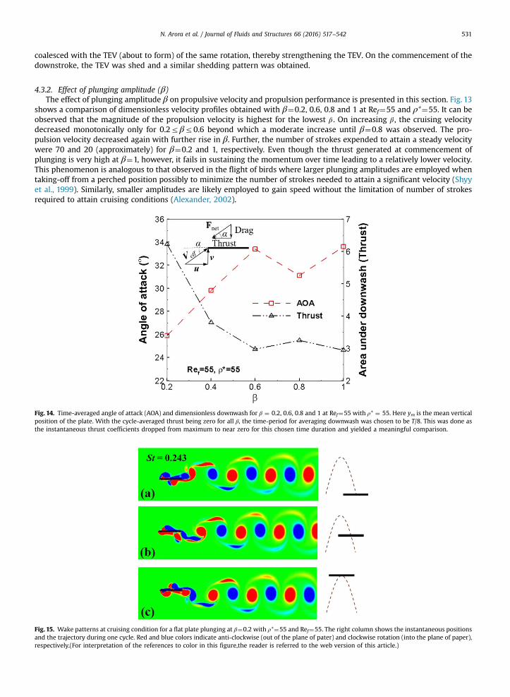
Fig. 14. Time-averaged angle of attack (AOA) and dimensionless downwash for β ¼ 0.2, 0.6, 0.8 and 1 at Ref¼55 with ρ* ¼ 55. Here ym is the mean verticalposition of the plate. With the cycle-averaged thrust being zero for all β, the time-period for averaging downwash was chosen to be T/8. This was done asthe instantaneous thrust coefficients dropped from maximum to near zero for this chosen time duration and yielded a meaningful comparison.

Fig. 15. Wake patterns at cruising condition for a flat plate plunging at β¼0.2 with ρ*¼55 and Ref¼55. The right column shows the instantaneous positionsand the trajectory during one cycle. Red and blue colors indicate anti-clockwise (out of the plane of pater) and clockwise rotation (into the plane of paper),respectively.(For interpretation of the references to color in this figure,the reader is referred to the web version of this article.)


To identify the reasons for non-monotonous behavior of propulsive velocity with increasing β, the angle of attack anddownwash for different β are compared in Fig. 14. The average angle of attack (AOA) for the self-propelled plate wascalculated as ( )∫α α¯ =

+d t T/

t

t T, where ( )α = − v utan /1 is the instantaneous angle of attack and =T T/2. Thus, a higher thrust

is expected to result in a higher cruising velocity leading to a smaller inclination with the flight direction. It is well knownthat jet formation behind a wing generates an opposite reaction force (Arora et al., 2014) and the downwash represents theamount of thrust generated (Freymuth, 1990; Lai and Platzer, 2000). As shown in Fig. 14, AOA and downwash increase anddecrease, respectively, when β≤ ≤0.2 0.6. However, AOA decreases (as downwash increases) at β = 0.8 due to constructivewing-wake interaction at the trailing edge resulting in an increase in the propulsion velocity at this amplitude. This peculiarbehavior of decrease in AOA and increase in thrust at β¼0.8 attributed to wing-wake interaction is explained further in thefollowing discussion.

The primary cause for high propulsion velocity and thrust at β¼0.2 can be understood by scrutiny of the flow patternsand force history. Fig. 15 shows the wake structures at cruising condition for β¼0.2 with Ref¼55 and ρ*¼55. As shown in

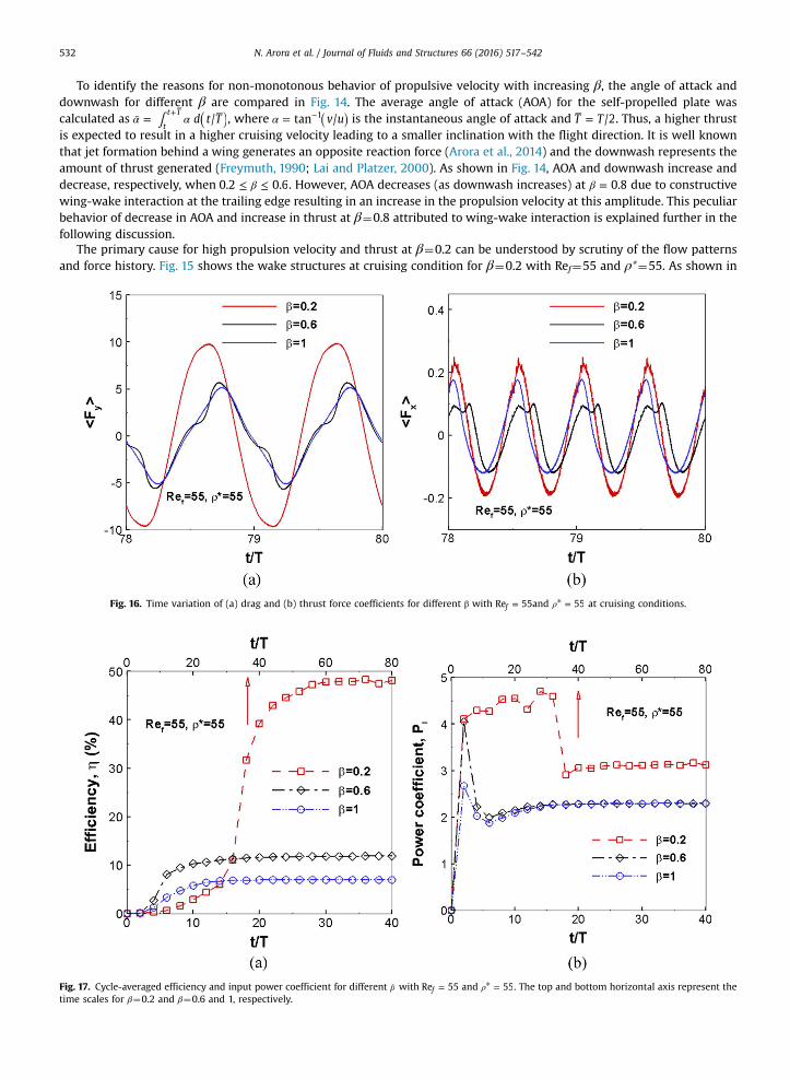
Fig. 16. Time variation of (a) drag and (b) thrust force coefficients for different β with =Re 55f and ρ* = 55 at cruising conditions.

Fig. 17. Cycle-averaged efficiency and input power coefficient for different β with =Re 55f and ρ* = 55. The top and bottom horizontal axis represent thetime scales for β¼0.2 and β¼0.6 and 1, respectively.


this figure, the vortex shedding behavior is very distinct from the patterns shown earlier for different Ref and with β¼0.6.With β¼0.2, the separation between the two opposite rotation vortices (one each during upstroke and downstroke) shedper stroke is a minimum. As can be observed from Fig. 15, stroke reversal occurs before the detached LEV could navigate tothe trailing edge or is swept away from the plate completely. At the beginning of upstroke the LEV was attached to the platewhich created a zone of low pressure at the leading edge. Simultaneously, a strong vortex dipole existed at the trailing edge.The presence of these opposite rotation vortices at the trailing edge assisted in creating a pressure imbalance across thechordwise direction. This pressure differential reflects in the form of a relatively larger thrust for β¼0.2, as is indicated inthe force coefficients shown in Fig. 16. Another important point to note from this figure is that the drag and thrust coef-ficients are the highest for β = 0.2. However, the drag coefficient decreases and becomes nearly similar for β = 0.6 and 1.On the other hand, the thrust coefficient decreases till β = 0.6 and increases thereafter.

This behavior of forces due to a high degree of wing–wake interaction echoes in the cycle-averaged efficiency and powercoefficients that are shown in Fig. 17. This figure highlights two aspects: (i) the cruising efficiency is highest for low β , and(ii) although a large change in power coefficient is observable when β changes from 0.2 to 0.6, no substantial change can benoticed when it increases from 0.6 to 1. Consequently, the behavior of input power is analogous to that of propulsionvelocity which was shown in Fig. 13.

Fig. 18. Flow field around the wing demonstrating induced downwash at t/T¼1/10 for (a) β ¼ 0.2, (b) β ¼ 0.6, (c) β ¼ 0.8 and (d) β ¼ 1.0 with Ref ¼ 55 andρ*¼55. The white arrows show the direction of movement of the plate.


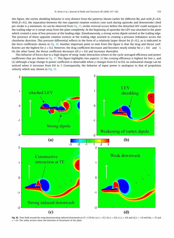
The increase in thrust between β¼0.6 to β¼0.8 was further investigated by examination of the vortex pattern aroundthe plate and the formation of vortex dipoles at the chosen amplitudes. As is shown in Fig. 18, for β¼0.6 it can be observedthat the shed LEV is sheared at the trailing edge by the ascending wing during stroke reversal. Due to this phenomenon,forward momentum is slightly hampered due to the weakening of vortex dipoles as the thrust coefficient and propulsionvelocity decrease. On the other hand, for β¼0.8 the shed LEV interacts with the wing exactly at the trailing edge. This shedLEV has enough time to completely advect downstream thereby inhibiting vortex shearing at the trailing edge, providing thedesired impetus to propel the plate faster and is indicative of greater area under downwash profile. On the other hand, forβ¼1 the LEV grows to such an extent that on shedding there is little interaction with the wing. As the amplitide is highest,the vortices with conflicting rotations are very distant from the trailing edge and the induced downwash due to thesedipoles is weak. Thus, the orientation and position of vortices during wing-wake interaction influences the generated thrust.Although reported in reference to ‘clap and fling’ (Arora et al., 2014), our assessment is that this is the only work in whichthe effect of wing-wake interaction with respect to induced downwash and strength of vortex dipole has been revealedwhich leads to increase or decrease in thrust.

Another important observation is that the separation between vortices increases with rise in β . Jones et al. (1998) statedthat the wavelength of vortex shedding is inversely proportional to reduced frequency k (where = =γ

β¯k Cu

St2). Since the

reduced frequency is inversely proportional to β , this justifies the increase in distance between oppositely directed vortices

Fig. 19. Comparison of (a) dimensionless instantaneous velocity and (b) non-dimensionalized trajectory for the flat plate plunging at ρ*¼10 and 100 withRef¼55 and β¼0.6 when starting from a state of rest. Also shown as dots are the distances reached at the end of specific strokes for the two density ratiosituations. By virtue of the plate's higher inertia, the undulations in the velocity are much lower at higher density ratio. Moreover, it takes much longer for ahigher inertia plate to reach cruising condition.


with increase in plunging amplitude. For the four cases shown in Fig. 18, the reduced frequencies are (a) k¼0.61, (b) k¼0.43,(c) k¼0.19 and (d) k¼0.16.

4.3.3. Effect of density ratio (ρ*)The effect of density ratio ρ*, with Ref and β held fixed, on the propulsion velocity and efficiency-power characteristics is

presented in this section. Fig. 19 shows a comparison of the time-evolution of velocity for ρ*¼10 and ρ*¼100 with Ref¼55and β¼0.6. Also shown are the trajectories of the plate for the two inertia cases. The results show that it takes more numberof strokes for the case of the higher inertia system to reach cruising condition. As shown in part (b) of this figure, a higherinertia body is slow to ‘react’ to the fluid forces and hence lags in the distance covered in the same number of strokes.However, the magnitude of velocity at cruising is nearly the same. Fig. 19 (b) also shows that the cruising velocity is attainedafter the plate has traversed distances of 68C and 147C for ρ*¼10 and 100, respectively. Finally, the undulations in thevelocity decrease with increase in density ratio by virtue of the plate's increasing inertia.

The role of plate inertia on aerodynamic force coefficients is depicted in Fig. 20. It can be observed that the magnitudesand evolvement of transverse forces with time are identical and indistinguishable. In addition, no difference in the flow fieldbehavior with change in ρ* was witnessed, which supported the above argument. These reasons affirm that the dragcoefficient is independent of ρ*; however, the thrust coefficient shows dependence only for lower values of this parameter.

Fig. 20. Time variation of (a) drag and (b) thrust force coefficients for different ρ* with =Re 55f and β = 0.6 at cruising conditions.

Fig. 21. Cycle-averaged efficiency and input power coefficient for different ρ*with =Re 55f and β = 0.6.


These results are unlike those for Ref and β that were shown earlier. As the drag coefficient and cruising velocity show weakdependence on density ratio, it can be expected that the power coefficient should also be independent of ρ*. This is cor-roborated in Fig. 21 which shows the cycle-averaged efficiency and power coefficients for various ρ*. On the other hand, thecycle-averaged efficiency can be observed to be increasing with increase in ρ*. Although not so apparent, the non-di-mensionalization method for efficiency and power coefficient used in this work can be shown to lead to two inferences tosupport this data as well; i.e., (a) the cycle-averaged power coefficient does not depend on ρ*, and (b) the efficiency isproportional to ρ*. However, this behavior is only valid when a cruising condition is attained. Prior to it, and as shown inFig. 22, a larger initial effort is required to propel a higher inertia body into locomotion. This figure shows that the areaunder the Pi�t/T curve i.e. measure of the total work done to reach cruising condition increases with ρ*. Lighter bodies areexpectedly more sensitive to fluid forces and hence respond to even small magnitude oscillations or disturbances, therebyreaching crusing conditions in a lesser number of strokes. On the other hand, higher inertia bodies are less susceptible toflow disturbances and variations and provide a relatively stable cruising velocity that is itself reached by expending greaterwork.

Fig. 22. Comparison of area under the instantaneous power curve (which represents dimensionless work) expended to reach the cruising conditionstarting from rest at ρ*¼10 (red) and ρ*¼100 (gray) with Ref¼55 and β¼0.6.(For interpretation of the references to color in this figure,the reader isreferred to the web version of this article.)

Fig. 23. Variation in cruising (a) propulsion efficiency oη4 and (b) input power coefficient oPi4 with change in Ref at β ¼ 0.2, 0.6 and 1 with ρ* ¼ 55.Inset in (a) shows the behavior of St versus Ref at same parameters.


4.4. Surrogate analysis

So far, an overview of the mechanism of propulsion of a rigid flat plate starting from a state of rest and plunging in aquiescent fluid along with the flow structures, pressure distribution around the plate and force histories had been pre-sented. The time-variation of efficiency and power was also highlighted. To understand the global response and determinethe global influence of kinematic parameters, we emphasize the surrogate modelling framework pursued in this work toassess their impact on input power and efficiency.

An initial DOE based upon the parameter range (refer Table 2) was built with 33 training points (15 using FCCD and 18using LHS). Using the formulated surrogates, however, the PRESSRMS for oη4 varied from 14% to 25% with Kriging and PRSreduced-order models. The PRESSRMS for oPi4 fared much worse with its range between 70–80%. A careful analysisshowed that the model fidelity was very poor for 10rρ*r25 and 0.6rβr1. Consequently, the DOE was further refined byincluding 22 new LHS sampling points such that sampling was significantly improved in the aforementioned range of ρ* andβ . With these 55 training points, the PRESSRMS with 3rd degree PRS for both oPi4 and oη4 reduced to 4.84% and 2.12%,respectively. The accuracy of the constructed surrogates was further tested by taking 5 random test points where thesurrogate predictions were compared to numerical model and the root mean square test errors were recorded to be 2.16%and 4.3% for oη4 and oPi4 , respectively. On an average, 40–50 h were required to run each simulation using parallelprogramming on a 24-core Intel Xeon Phi processor for the large domain size considered in this work. Since these cross-validation and test errors were less than 5%, the model was considered to have attained satisfactory fidelity. The formulatedsurrogates were frozen to conduct further analyses. The polynomial expression obtained through surrogate modelling foroη4 and oPi4 are given in Appendix which had the goodness of fit Radj

2 as 0.996 and 0.977, respectively.Similar to oη4 and oPi4 , a surrogate model for Strouhal number based on the second-order kriging spline corre-

lation with the same DOE and a PRESSRMS of 4.6% was also formulated. Since this study has been performed on a self-propelled wing, the forward translational velocity or Strouhal number is dependent on the plunging parameters and cannotbe varied independently (unlike studies in which the wing flapped at a fixed position where St could be varied by changingthe speed of oncoming flow). Therefore, this kriging model enabled us to examine the behavior of oη4 and oPi4 as afunction of St as is shown in Fig. 23. The inset shows the variation in St with Ref at ρ*¼55 and β¼0.2, 0.6 and 1. Althoughthere is a direct relationship between Strouhal number and flapping Reynolds number ( =St 2Re /Ref u), St decreased con-tinuously with increase in Ref. This is reflected in the continuous increase in efficiency with a decrease in St, with therelationship being nearly linear for higher values of β. Likewise, input power shows a rapid increase with decreasing St(except at β¼0.2, where a sharp change is obtained when St approaches 0.2). In addition, Taylor et al. (2003) stated thatflying animals are naturally calibrated to cruise at a Strouhal number lying between 0.2 and 0.4 for efficient flight. Analogousto this finding, 85% of the cases (from simulations and surrogate model) exhibited Strouhal numbers that fell in the efficientflight range (also evident in Fig. 23). The remaining cases where St was off-limit lied in the threshold region (high β, low ρ*and Ref �20) that represented the transition phase from unsteady to steady propulsion velocity (i.e. aperiodic to periodicvortex shedding). This transition zone was characterized by a deflective wake pattern and which has been discussed in anearlier section.

4.5. Sensitivity analysis

A sensitivity analysis was also performed using the formulated surrogate models. Fig. 24 shows the sensitivity indices ofthe kinematic parameters on efficiency and input power. The main sensitivity index quantifies the direct influence of

Fig. 24. Global sensitivity analysis of efficiency oη4 and power coefficient oPi4 showing main and total sensitivity indices.


individual parameters on the change in dependent variable, whereas the total index specifies the joint or collective impactof the input variables on the objective function. The deficit of these two indices is a measure of the cross interaction or theinterconnectivity of the parameters.

The sensitivity analysis of efficiency showed that β is the most influential parameter, with its main index being largestamongst all the three variables. Moreover, β and ρ* had a coupled effect as together they had a significant impact onefficiency. This is clearly noticeable in the total sensitivity indices of β and ρ* which are higher than their main counterpartsby about 12.5%, implying the extent of interaction of these two variables is quite significant (for Ref, there was only amarginal increase in total sensitivity of mere 3%). On the contrary, Ref does not influence efficiency as much as otherkinematic parameters.

As far as the input power coefficient is concerned, Ref had the maximum sensitivity index making it to be the mostdominant parameter. The sensitivity analysis also confirms the earlier argument of insignificant effect of density ratio.Nevertheless, ρ* could not be ignored as the sensitivity analysis of efficiency established it to be a crucial parameter as well.

4.6. Pareto front

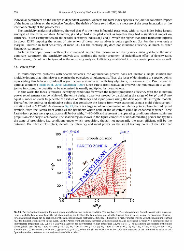
In multi-objective problems with several variables, the optimization process does not involve a single solution butmultiple designs that minimize or maximize the objectives simultaneously. Thus, the locus of dominating or superior pointsrepresenting this behavior (trade-off region between minima of conflicting objectives) is known as the Pareto-front oroptimal solutions (Trizila et al., 2011; Miettinen, 1999). Since Pareto-front evaluation involves the minimization of all ob-jective functions, the quantity to be maximized is usually multiplied by negative one.

In this work, the focus is towards identifying conditions for which the highest propulsion efficiency with the minimumpower requirements can be achieved. The entire design space was probed by partitioning the range of Ref, ρ* and β intoequal number of levels to generate the values of efficiency and input power using the developed PRS surrogate models.Thereafter, the optimal or dominating points that constitute the Pareto-front were extracted using a multi-objective opti-mization tool in MATLAB

s

. As shown in Fig. 25, there is a large set of non-dominated or inferior points (characterized by redsymbols) with the Pareto-front acting as the periphery where none of the objectives could be enhanced together. ThesePareto-front points were spread across all Ref but with ρ*�80–100 and represent the operating conditions where maximumpropulsion efficiency is achievable. The shaded region shown in the figure comprises of non-dominating points and typifiesthe zone of propulsion, i.e., conditions under which propulsion, though not necessarily the most efficient, will be theoutcome. The filled circles (black) denote the efficiency and input power for the set of training points of the DOE that

Fig. 25. Pareto-front optimization for input power and efficiency at cruising condition. The symbols (red) are data obtained from the constructed surrogatemodels with the Pareto-front being the set of dominating points. Thus, the Pareto-front provides the locus of flow scenarios where the maximum efficiencyfor a given input power can be realized. For the same input power coefficient, efficiency is higher for a higher inertia system, with the maximum reachednear the highest ρ*considered in this work. On the Pareto-front, efficiency increases with increasing Ref and decreasing β . ‘Zone A′ is defined for low tointermediate amplitudes (i.e., β≤ ≤0.2 0.6) while ‘Zone B′ for intermediate to high amplitudes (i.e, β≤ ≤0.6 1). The parametric coordinates of the filledcircles (black) are: (a) Ref ¼100, ρ*¼100, β¼0.2, (b) Ref ¼20, ρ*¼100, β¼0.2, (c) Ref ¼100, ρ*¼10, β¼0.2, (d) Ref ¼20, ρ*¼10, β¼0.2, (e) Ref ¼100,ρ*¼100, β¼1, (f) Ref ¼100, ρ*¼10, β¼1, (g) Ref ¼20, ρ*¼100, β¼1.0 and (h) Ref ¼20, ρ*¼10, β¼1.(For interpretation of the references to color in thisfigure,the reader is referred to the web version of this article.)


correspond to FCCD sampling. The maximum and minimum propulsion efficiency are obtained at a (Ref ¼100, ρ*¼100,β¼0.2) and h (Ref ¼20, ρ*¼10, β¼1), respectively, which lie at the diagonally opposite corners of the DOE.

As is shown in the figure, a key outcome from an analysis of the Pareto-front is that the set of optimal points could besplit into two zones, A & B. ‘Zone A’ corresponds to low to intermediate amplitudes, while ‘zone B′ is for intermediate to highamplitudes. Further, parametric analysis shows that high efficiency, though with requirement of large input power, isachievable in zone A while zone B can only yield scenarios corresponding to low input power and efficiency. This Pareto-front indicates that the best efficiency can be achieved only in high inertia systems by increasing both the flapping Reynoldsnumber and decreasing the amplitude ratio, though at the expense of greater input power. Clearly, wing-wake interactionwhich occurs due to weaker vortex dissipation at high Ref and presence of vortex dipole at the trailing edge at low am-plitudes acting in tandem can lead to achievement of high propulsion efficiency.

5. Conclusions

The present work was directed towards characterizing the fluid mechanics associated with a self-propelled-heaving rigidflat plate in a quiescent medium. In this regard, a shifting discontinuous-grid-block around a moving solid body based onthe multi-relaxation time lattice Boltzmann method was employed. A parametric study was performed to characterize theinfluence of Reynolds number Ref, plunging amplitude β and density ratio ρ* on the forward flight efficiency and powerrequirements for the flat plate at cruising conditions. In addition, the impact of these variables on propulsion velocity waselucidated with the help of flow structures and their interaction with the wing.

Simulations exhibited that attainment of cruising condition resulted in a periodically varying thrust coefficient that owedthis behavior to the pressure at leading and trailing edges alternating between maximum and minimum values. This wasshown to depend on the kinematics and occurred due to opposite-orientation vortices getting shed during upstroke anddownstroke. Various periodic vortex shedding characteristics of the plunging plate were observed that led to modification ofthe angle of attack as a result of wing-wake interaction and downward jet.

It was also revealed that with increase in flapping Reynolds number (Ref), the propulsion velocity (or Reu), cruisingefficiency and input power coefficient increased due to an increased degree of wing-wake interaction. At low Ref, vorticeswere shed at an angle (indicative of transition phase from unsteady to quasi-steady propulsion) which quickly dissipated,whereas at high values of Ref a long, equally spaced and oppositely directed symmetric trail was observed. At low β, a strongvortex dipole prevailed at the trailing edge along with an attached LEV that led to maximum thrust generation and highestcruising efficiency. For higher β, the position and orientation of vortices during stroke reversal dictated the productive ordestructive effect of wing-wake interaction leading to an increase or decrease in the angle of attack and downwash. For thedensity ratio (ρ*), the overall energy expended to attain a cruising condition starting from rest was much higher for higherinertia bodies as a larger number of plunging strokes was required to reach this stage. Lastly, cruising efficiency increasedwith increase in ρ* as it became directly proportional to wing inertia.

Surrogate modelling was employed to assess and identify the optimum conditions for forward flight. Based on theformulated surrogate models of efficiency and input power requirements for forward flight, a Pareto-optimal solution whichdescribed the tradeoff between these two competing objectives was obtained. The Pareto-front analysis highlighted that theset of optimal points could be split into two zones corresponding to low and high amplitude kinematics. This Pareto-frontindicated that wing-wake interaction which occurs at low β and high Ref due to weak vortex dissipation and presence ofvortex dipole at the trailing edge acting in tandem can lead to achieving high propulsion efficiency in high inertia systems.This Pareto-front provided guidance on the maximum efficiency that can be attained for a given input power, therebydefining the ideal operating range and is expected to be of significance for the design of next generation flapping wingMAVs.

Acknowledgement

N.A. and A.G. acknowledge the financial support received from the Aeronautics Research and Development Board (ARDB)under SIGMA project No. 1705. The authors also thank the IIT Delhi HPC facility for computational resources.

Appendix

Multi-Relaxation Time LBM

In this method, the distribution function f (as defined in the SRT model) in the discrete velocity space F is mapped ontothe moment space K by using a transformation matrix M (Arora et al., 2016), i.e.

^ = = ^ ( )−f Mf f M fand 251


where f is a column matrix consisting of moments of the velocity distribution function (each row vector) which representsthe following quantities in two-dimensional space:

ρ ε^ = ( )⎡⎣ ⎤⎦f e j q j q p p, , , , , , , , 26x x y y xx xy

T

where ρ is the density, e signifies the kinetic energy, ε epitomizes the square of kinetic energy, jx and jy are the x and ycomponents of the momentum flux, qx and qy are related to the x and y components of energy density, and pxx and pxy referto the diagonal and off-diagonal terms in viscous stress tensor.

The equilibrium values for the non-conserved moments can be obtained from the conserved moments ρ and j ( jx and jy)(Arora et al., 2016) as

( )ρρ

= − + +( )

e j j23

27eq

x y2 2

( )ε ρρ

= − +( )

j j3

28eq

x y2 2

= − = − ( )q j q j, 29xeq

x yeq

y

( )ρ= −

( )p j j

130xx

eqx y2 2

ρ=

( )p j j

131xy

eqx y

The transformation matrix for the D2Q9 model is given by Arora et al. (2016)

=

− − − − −− − − −

− − −− − −

− − −− − −− −

− − ( )

⎡

⎣

⎢⎢⎢⎢⎢⎢⎢⎢⎢⎢⎢

⎤

⎦

⎥⎥⎥⎥⎥⎥⎥⎥⎥⎥⎥

M

1 1 1 1 1 1 1 1 14 1 1 1 1 2 2 2 2

4 2 2 2 2 1 1 1 10 1 0 1 0 1 1 1 10 2 0 2 0 1 1 1 10 0 1 0 1 1 1 1 10 0 2 0 2 1 1 1 10 1 1 1 1 0 0 0 00 0 0 0 0 1 1 1 1 32

The collision process is performed in the K space which is as follows:

^* = ^ − ^ − ^

( )⎡⎣⎢

⎤⎦⎥f f S f f

33

eq

Table 4Third-degree polynomial coefficients obtained from surrogate modelling for oη4 and oPi4 .

Coefficient η Pi

a0 4.55 3.05a1 20.93 �0.50a2 49.24 �0.16a3 �33.98 �5.63a4 �19.84 0.71a5 56.72 1.13a6 �32.30 3.27a7 1.62 �0.23a8 �119.78 �0.19a9 74.62 9.27a10 3.82 �0.03a11 �16.63 �0.45a12 19.78 �1.52a13 1.99 �0.62a14 �37.78 �0.01a15 9.81 �1.30a16 �14.15 0.33a17 17.22 �0.14a18 72.52 0.47a19 �44.80 �5.07


where ^*f is the post collision operator, and S is the diagonal relaxation time matrix

= [ ] ( )S diag s s s s s s s s s, , , , , , , , 341 2 3 4 5 6 7 8 9

where s1¼s4¼s6 ¼ 0 (relaxation time for the conserved quantities).The moments f are transformed back and thus the advection step is carried out in the F space on the distribution

function f . Thus, Eq. (33) can be written as

˜ = ^ − ^ − ^( )

− − ⎡⎣⎢

⎤⎦⎥f M f M S f f

35

eq1 1

where f is the post collision distribution function in F space which are then streamed to the neighboring nodes in directionof the lattice velocities.

6.1. Surrogate model

The 3rd degree polynomial expression for oη4 and oPi4 is as follows

η ρ β ρ β ρ ρ β β ρ

β ρ ρ β β ρ ρ β ρ β β

= + + * + + + * + + * + * + + + *

+ + * + * + + * + * + * + ( )

P a a a a a a a a a a a a

a a a a a a a a

, Re Re Re Re Re Re

Re Re Re Re 36

i 0 1 f 2 3 4 f2

5 f 6 f 72

8 92

10 f3

11 f2

12 f2

13 f2

14 f 15 f2

163

172

182

193

The coefficients as obtained from the PRS surrogate model for normalized values of Ref, ρ* and β (range scaled between0 and 1) are given in Table 4.

References

Alben, S., Shelley, M., 2005. Coherent locomotion as an attracting state for a free flapping body. Proc. Natl. Acad. Sci. 102, 11163–11166.Alexander, D.E., 2002. In: Nature's FlyersThe John Hopkins University Press, Baltimore.Anderson, J.M., Streitlien, K., Barrett, D.S., Triantafyllou, M.S., 1998. Oscillating foils of high propulsive efficiency. J. Fluid Mech. 360, 41–72.Aono, H., Gupta, A., Qi, D., and Shyy, W., The Lattice Boltzmann Method for Flapping Wing Aerodynamics, In: Proceedings of the 40th AIAA Fluid Dynamics Conference

and Exhibit, June 2010, Chicago, Illinois, USA.Arora, N., Gupta, A., Shyy, W., 2016. A shifting discontinuous-grid-block lattice Boltzmann method for moving boundary simulations. Comput. Fluids 125, 59–70.Arora, N., Gupta, A., Sanghi, S., Aono, H., Shyy, W., 2014. Lift-drag and flow structures associated with the ‘clap and fling’ motion. Phys. Fluids 26, 071906.Benkherouf, T., Mekadem, M., Oualli, H., Hanchi, S., Keirsbulck, L., Labraga, L., 2011. Efficiency of an auto-propelled flapping airfoil. J. Fluids Struct. 27, 552–566.Betz, A., 1912. Ein Beitrag zur Erklarung des Segelfluges. Zeitsch. Flugtechnik Motorluftschiffahrt 3, 269–272.Chen, S., Doolen, G.D., 1998. Lattice Boltzmann method for fluid flows. Annu. Rev. Fluid Mech. 30, 329–364.Chin, D.D., Lentink, D., 2016. Flapping wing aerodynamics: from insects to vertebrates. J. Exp. Biol. 219, 920–932.Croon, De, G. C. H. E, Percin, M., Remes, B.D.W., Ruijsink, R., De Wagter, C., 2016. The DelFly: Design, Aerodynamics, and Artificial Intelligence of a Flapping Wing Robot.

Springer, London.Dickinson, M.H., Lehmann, F.-O., Sane, S.P., 1999. Wing rotation and the aerodynamic basis of insect flight. Science 284, 1954–1960.Freymuth, P., 1988. Propulsive vortical signature of plunging and pitching airfoils. AIAA J. 26, 881–883.Freymuth, P., 1990. Thrust generation by an airfoil in hover modes. Exp. Fluids 9, 17–24.Fuller, S.B., Karpelson, M., Censi, A., Ma, K.Y., Wood, R.J., 2014. Controlling free flight of a robotic fly using an onboard vision sensor inspired by insect Ocelli. J. R. Soc.

Interface 11, 0281.Goel, T., Dorney, D.J., Haftka, R.T., Shyy, W., 2008. Improving the hydrodynamic performance of diffuser vanes via shape optimization. Comput. Fluids 37, 705–723.Hu, J., Xiao, Q., 2014. Three-dimensional effects on the translational locomotion of a passive heaving wing. J. Fluids Struct. 46, 77–88.Jones, K.D., Dohring, C.M., Platzer, M.F., 1998. Experimental and computational investigation of the Knoller–Betz effect. AIAA J. 36, 1240–1246.Kang, C.K., Shyy, W., 2013. Scaling law and enhancement of lift generation of an insect-size hovering flexible wing. J. R. Soc. Interface 10, 0361.Kang, C.K., Shyy, W., 2014. Analytical model for instantaneous lift and shape deformation of an insect-scale flapping wing in hover. J. R. Soc. Interface 11, 0933.Kang, C.K., Aono, H., Cesnik, C.E.S., Shyy, W., 2011. Effects of flexibility on the aerodynamic performance of flapping wings. J. Fluid Mech. 689, 32–74.Katzmayr, R., Effect of Periodic Changes of Angle of Attack on Behavior of Airfoils, (translated From Zeitschrift fur Flugtechnik und Motorluftschiffahrt, March 31, 1922,

pp. 80–82, and April 13, 1922, pp. 95–101.Keennon, M., Klingebiel, K., Won, H., and Andriukov, A., Development of the Nano hummingbird: A tailless flapping wing micro air vehicle. In: Proceedings of the 50th

AIAA Aerospace Sciences Meeting, Reston, Virginia, USA: January 2012.Kern, S., Koumoutsakos, P., 2006. Simulations of optimized anguilliform swimming. J. Exp. Biol. 209, 4841–4857.Knoller, R., 1909. Die Gesetze des Liftwiderstandes. Flug- und Motortechnik (Wiener) 3 (21), 1–7.Ladd, A.J.C., 1994. Numerical simulations of particulate suspensions via a discretized boltzmann equation. Part 1. Theoretical Foundation. J. Fluid Mech. 271, 285–309.Lai, J.C.S., Platzer, M.F., 2000. Characteristics of a plunging airfoil at zero freestream velocity. AIAA J. 39, 531–534.Lallemand, P., Luo, L.-S., 2003. Lattice Boltzmann method for moving boundaries. J. Comput. Phys. 184, 406–421.Lee, J., Choi, H., Kim, H.-Y., 2015. A scaling law for the lift of hovering insects. J. Fluid Mech. 782, 479–490.Lewin, G.C., Haj-Hariri, H., 2003. Modelling thrust generation of a two-dimensional heaving airfoil in a viscous flow. J. Fluid Mech. 492, 339–362.Lu, X.-Y., Liao, Q., 2006. Dynamic responses of a two-dimensional flapping foil motion. Phys. Fluids 18, 098104.Ma, K. Y., Chirarattananon, P., and Wood, R.J., Design and Fabrication of an Insect-scale Flying Robot for Control Autonomy. In: Proceedings of the IEEE/RSJ Inter-

national Conference on Intelligent Robots and Systems (IROS), Hamburg, Germany: 2015.Miettinen, K.M., 1999. Nonlinear Multiobjective Optimization, BostonKluwer Academic.Muller, T.J., 2001. Fixed and flapping wing aerodynamics for micro air vehicle applications. AIAA Prog. Astronaut. Aeronaut, 195.Quiepo, N.V., Haftka, R.T., Shyy, W., Goel, T., Vaidyanathan, R., Tucker, P.K., 2005. Surrogate-based analysis and optimization. Prog. Aerosp. Sci. 41, 1–28.Quinn, D.B., Lauder, G.V., Smits, A.J., 2013. Scaling the propulsive performance of heaving flexible panels. J. Fluid Mech. 738, 250–267.Sane, S.P., 2003. The aerodynamics of insect flight. J. Exp. Biol. 206, 4191–4208.Schultz, W.W., Webb, P.W., 2002. Power requirements of swimming: do new methods resolve old questions? Integr. Comp. Biol. 42, 1018–1025.Shyy, W., Berg, M., Ljungqvist, D., 1999. Flapping and flexible wings for biological and micro air vehicles. Prog. Aerosp. Sci. 35, 155–205.Shyy, W., Papila, N., Vaidyanathan, R., Tucker, K., 2001. Global design optimization for aerodynamics and rocket propulsion components. Prog. Aerosp. Sci. 37, 59–118.Shyy, W., Trizila, P., Kang, C., Aono, H., 2009. Can Tip vortices enhance lift of a flapping wing? AIAA J. 47, 289–293.Shyy, W., Aono, H., Kang, C.-K., Liu, H., 2013. In: An Introduction to Flapping Wing AerodynamicsCambridge University Press, New York.

http://refhub.elsevier.com/S0889-9746(16)30304-8/sbref1





































































Shyy, W., Lian, Y., Tang, J., Viieru, D., Liu, H., 2008. In: Aerodynamics of Low Reynolds Number FlyersCambridge University Press, New York.Shyy, W., Kang, C.-k, Chirarattananon, P., Ravi, S., Liu, H., 2016. Aerodynamics, sensing and control of insect-scale flapping wing-flight. Proc. R. Soc. A 472, 20150712.Shyy, W., Cho, Y.-C., Du, W., Gupta, A., Tseng, C.-C., Sastry, A.M., 2011. Surrogate-based modeling and dimension reduction techniques for multi-scale mechanics

problems. Acta Mech. Sin. 27, 845–865.Shyy, W., Aono, H., Chimakurthi, S.K., Trizila, P., Kang, C.K., Cesnik, C.E.S., Liu, H., 2010. Recent progress in flapping wing aerodynamics and aeroelasticity. Prog. Aerosp.

Sci. 46, 284–327.Succi, S., 2001. In: The Lattice Boltzmann Equation for Fluid Dynamics and BeyondOxford University Press, New York.Taylor, G.K., Nudds, R.L., Thomas, A.L.R., 2003. Flying and swimming animals cruise at a strouhal number tuned for high power efficiency. Nature 425, 707–711.Triantafyllou, M.S., Triantafyllou, G.S., Gopalkrishnan, R., 1991. Wake mechanics for thrust generation in oscillating airfoils. Phys. Fluids 3 (12), 1989–1993.Trizila, P., Kang, C.-K., Aono, H., Visbal, M., Shyy, W., 2011. Low Reynolds number aerodynamics of a flapping rigid flat plate. AIAA J. 49, 806–823.Tsai, B.-J., Fu, Y.-C., 2009. Design and aerodynamic analysis of a flapping-wing micro aerial vehicle. Aerosp. Sci. Technol. 13, 383–392.Vandenberghe, N., Zhang, J., Childress, S., 2004. Symmetry breaking leads to forward flapping flight. J. Fluid Mech. 506, 147–155.Vandenberghe, N., Childress, S., Zhang, J., 2006. On unidirectional flight of a free flapping wing. Phys. Fluids 18, 014102.Zhang, X., Ni, S., Wang, S., He, G., 2009. Effects of geometric shape on the hydrodynamics of a self-propelled flapping foil. Phys. Fluids 21, 103302.






















Journal of Fluids and Structures - Indian Institute of...

Documents

Transcript of Journal of Fluids and Structures - Indian Institute of...