ARTICLE IN PRESS

JID: FINEC [m3Gdc; December 14, 2018;13:23 ]

Journal of Financial Economics xxx (xxxx) xxx

Contents lists available at ScienceDirect

Journal of Financial Economics

journal homepage: www.elsevier.com/locate/jfec

Indexing and stock market serial dependence around the

world

�

Guido Baltussen

a , ∗, Sjoerd van Bekkum

a , Zhi Da

b

a Erasmus University, Finance Group/Erasmus School of Economics, Burgemeester Oudlaan 50, Rotterdam 2518HD, Netherlands b University of Notre Dame, 239 Mendoza College of Business, Notre Dame, IN 46556, USA

a r t i c l e i n f o

Article history:

Received 22 December 2016

Revised 19 June 2017

Accepted 2 July 2017

Available online xxx

JEL classification:

G12

G14

G15

Keywords:

Return autocorrelation

Stock market indexing

Exchange-traded funds (ETFs)

Arbitrage

a b s t r a c t

We show a striking change in index return serial dependence across 20 major market

indexes covering 15 countries in North America, Europe, and Asia. While many studies

find serial dependence to be positive until the 1990s, it switches to negative since the

20 0 0s. This change happens in most stock markets around the world and is both statisti-

cally significant and economically meaningful. Further tests reveal that the decline in serial

dependence links to the increasing popularity of index products (e.g., futures, exchange-

traded funds, and index mutual funds). The link between serial dependence and indexing

is not driven by a time trend, holds up in the cross section of stock indexes, is confirmed

by tests exploiting Nikkei 225 index weights and Standard & Poor’s 500 membership,

and in part reflects the arbitrage mechanism between index products and the underlying

stocks.

© 2018 Elsevier B.V. All rights reserved.

1. Introduction

Since the 1980s, many studies have examined the mar-

tingale property of asset prices and shown positive serial

dependence in stock index returns. Several explanations for

this phenomenon have been posited such as market mi-

crostructure noise (stale prices) and slow information dif-

fusion (the partial adjustment model). In this paper, we

provide systematic and novel evidence that serial depen-

dence in index returns has turned significantly negative

more recently across a broad sample of 20 major market

indexes covering 15 countries in North America, Europe,

� We thank Nishad Matawlie and Bart van der Grient for excel-

lent research assistance, and thank Zahi Ben-David, Heiko Jacobs, Jef-

frey Wurgler, and seminar participants at Erasmus University, Maastricht

University, and the Luxembourg Asset Management Summit for useful

comments. Any remaining errors are our own. ∗ Corresponding author.

E-mail address: baltussen@ese.eur.nl (G. Baltussen).

https://doi.org/10.1016/j.jfineco.2018.07.016

0304-405X/© 2018 Elsevier B.V. All rights reserved.

Please cite this article as: G. Baltussen, S. van Bekkum and Z. Da

world, Journal of Financial Economics, https://doi.org/10.1016/j.jfi

and the Asia-Pacific. Negative serial dependence implies

larger and more frequent index return reversals that can-

not be directly accounted for by traditional explanations.

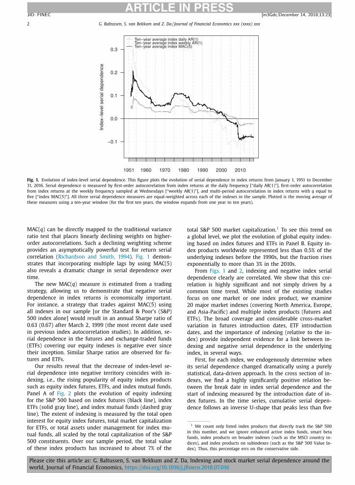
Our key result is illustrated in Fig. 1 , which plots

several measures for serial dependence in stock market

returns averaged over a ten-year rolling window. While

first-order autocorrelation [AR(1)] coefficients from daily

returns have traditionally been positive, fluctuating around

0.05 from 1951, they have been steadily declining ever

since the 1980s and switched sign during the 20 0 0s. They

have remained negative ever since.

This change is not limited to first-order daily autocor-

relations. For instance, AR(1) coefficients in weekly returns

evolved similarly and switched sign even before 20 0 0. Be-

cause we do not know a priori which lag structure com-

prehensively measures serial dependence, we examine a

novel measure for serial dependence, multi-period auto-

correlation [MAC( q )], that incorporates serial dependence

at multiple (that is, q ) lags. For instance, MAC(5) incor-

porates daily serial dependence at lags one through four.

, Indexing and stock market serial dependence around the

neco.2018.07.016

2 G. Baltussen, S. van Bekkum and Z. Da / Journal of Financial Economics xxx (xxxx) xxx

ARTICLE IN PRESS

JID: FINEC [m3Gdc; December 14, 2018;13:23 ]

Fig. 1. Evolution of index-level serial dependence. This figure plots the evolution of serial dependence in index returns from January 1, 1951 to December

31, 2016. Serial dependence is measured by first-order autocorrelation from index returns at the daily frequency [“daily AR(1)”], first-order autocorrelation

from index returns at the weekly frequency sampled at Wednesdays [“weekly AR(1)”], and multi-period autocorrelation in index returns with q equal to

five [“index MAC(5)”]. All three serial dependence measures are equal-weighted across each of the indexes in the sample. Plotted is the moving average of

these measures using a ten-year window (for the first ten years, the window expands from one year to ten years).

1 We count only listed index products that directly track the S&P 500

in this number, and we ignore enhanced active index funds, smart beta

funds, index products on broader indexes (such as the MSCI country in-

dices), and index products on subindexes (such as the S&P 500 Value In-

dex). Thus, this percentage errs on the conservative side.

MAC( q ) can be directly mapped to the traditional variance

ratio test that places linearly declining weights on higher-

order autocorrelations. Such a declining weighting scheme

provides an asymptotically powerful test for return serial

correlation ( Richardson and Smith, 1994 ). Fig. 1 demon-

strates that incorporating multiple lags by using MAC(5)

also reveals a dramatic change in serial dependence over

time.

The new MAC( q ) measure is estimated from a trading

strategy, allowing us to demonstrate that negative serial

dependence in index returns is economically important.

For instance, a strategy that trades against MAC(5) using

all indexes in our sample [or the Standard & Poor’s (S&P)

500 index alone] would result in an annual Sharpe ratio of

0.63 (0.67) after March 2, 1999 (the most recent date used

in previous index autocorrelation studies). In addition, se-

rial dependence in the futures and exchange-traded funds

(ETFs) covering our equity indexes is negative ever since

their inception. Similar Sharpe ratios are observed for fu-

tures and ETFs.

Our results reveal that the decrease of index-level se-

rial dependence into negative territory coincides with in-

dexing, i.e., the rising popularity of equity index products

such as equity index futures, ETFs, and index mutual funds.

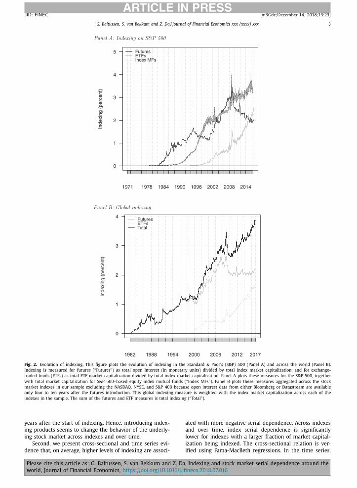
Panel A of Fig. 2 plots the evolution of equity indexing

for the S&P 500 based on index futures (black line), index

ETFs (solid gray line), and index mutual funds (dashed gray

line). The extent of indexing is measured by the total open

interest for equity index futures, total market capitalization

for ETFs, or total assets under management for index mu-

tual funds, all scaled by the total capitalization of the S&P

500 constituents. Over our sample period, the total value

of these index products has increased to about 7% of the

Please cite this article as: G. Baltussen, S. van Bekkum and Z. Da

world, Journal of Financial Economics, https://doi.org/10.1016/j.jfi

total S&P 500 market capitalization. 1 To see this trend on

a global level, we plot the evolution of global equity index-

ing based on index futures and ETFs in Panel B. Equity in-

dex products worldwide represented less than 0.5% of the

underlying indexes before the 1990s, but the fraction rises

exponentially to more than 3% in the 2010s.

From Figs. 1 and 2 , indexing and negative index serial

dependence clearly are correlated. We show that this cor-

relation is highly significant and not simply driven by a

common time trend. While most of the existing studies

focus on one market or one index product, we examine

20 major market indexes (covering North America, Europe,

and Asia-Pacific) and multiple index products (futures and

ETFs). The broad coverage and considerable cross-market

variation in futures introduction dates, ETF introduction

dates, and the importance of indexing (relative to the in-

dex) provide independent evidence for a link between in-

dexing and negative serial dependence in the underlying

index, in several ways.

First, for each index, we endogenously determine when

its serial dependence changed dramatically using a purely

statistical, data-driven approach. In the cross section of in-

dexes, we find a highly significantly positive relation be-

tween the break date in index serial dependence and the

start of indexing measured by the introduction date of in-

dex futures. In the time series, cumulative serial depen-

dence follows an inverse U-shape that peaks less than five

, Indexing and stock market serial dependence around the

neco.2018.07.016

G. Baltussen, S. van Bekkum and Z. Da / Journal of Financial Economics xxx (xxxx) xxx 3

ARTICLE IN PRESS

JID: FINEC [m3Gdc; December 14, 2018;13:23 ]

Fig. 2. Evolution of indexing. This figure plots the evolution of indexing in the Standard & Poor’s (S&P) 500 (Panel A) and across the world (Panel B).

Indexing is measured for futures (“Futures”) as total open interest (in monetary units) divided by total index market capitalization, and for exchange-

traded funds (ETFs) as total ETF market capitalization divided by total index market capitalization. Panel A plots these measures for the S&P 500, together

with total market capitalization for S&P 500–based equity index mutual funds (“Index MFs”). Panel B plots these measures aggregated across the stock

market indexes in our sample excluding the NASDAQ, NYSE, and S&P 400 because open interest data from either Bloomberg or Datastream are available

only four to ten years after the futures introduction. This global indexing measure is weighted with the index market capitalization across each of the

indexes in the sample. The sum of the futures and ETF measures is total indexing (“Total”).

years after the start of indexing. Hence, introducing index-

ing products seems to change the behavior of the underly-

ing stock market across indexes and over time.

Second, we present cross-sectional and time series evi-

dence that, on average, higher levels of indexing are associ-

Please cite this article as: G. Baltussen, S. van Bekkum and Z. Da

world, Journal of Financial Economics, https://doi.org/10.1016/j.jfi

ated with more negative serial dependence. Across indexes

and over time, index serial dependence is significantly

lower for indexes with a larger fraction of market capital-

ization being indexed. The cross-sectional relation is ver-

ified using Fama-MacBeth regressions. In the time series,

, Indexing and stock market serial dependence around the

neco.2018.07.016

4 G. Baltussen, S. van Bekkum and Z. Da / Journal of Financial Economics xxx (xxxx) xxx

ARTICLE IN PRESS

JID: FINEC [m3Gdc; December 14, 2018;13:23 ]

2 This mechanism is underpinned by theory in Leippold et al. (2015) .

Bhattacharya and O’Hara (2015) demonstrate theoretically that similar

shock propagation can occur due to imperfect learning about informed

trades in the index product. For further intuition on the arbitrage mecha-

nism, see Ben-David et al. (2018) Fig. 1 , and Greenwood (2005) .

the significantly negative relation survives when we re-

move the time trend, regress quarterly changes in MAC(5)

on quarterly changes in indexing, or add index fixed ef-

fects. Thus, increases in indexing are associated with de-

creases in serial dependence that go beyond sharing a

common time trend, and the link cannot be explained by

differences between stock markets.

The link between indexing and index-level negative se-

rial dependence could be spurious. For instance, higher de-

mand for trading the market portfolio results in correlated

price pressure on all stocks, which could also make index

serial dependence turn negative. In other words, index se-

rial dependence could have changed due to market-wide

developments, regardless of whether index products have

been introduced or not. One could even argue that the fu-

tures introduction date is endogenous and futures trading

is introduced with the purpose of catering to market-level

order flow. In this paper, we identify the impact of index-

ing on the index by comparing otherwise similar stocks

with very different indexing exposure that arise purely

from the specific design of the index. We do this in two

ways.

First, we exploit the relative weighting differences of

Japanese stocks between the Nikkei 225 index and the

Tokyo Stock Price Index (TOPIX). Because the Nikkei 225

is price weighted and the TOPIX is value weighted, some

small stocks are overweighted in the Nikkei 225 when

compared with their market capitalization-based weight

in the TOPIX. Greenwood (2008) finds that overweighted

stocks receive proportionally more price pressure and uses

overweighting as an instrument for non-fundamental index

demand that is uncorrelated with information that gets re-

flected into prices. We employ the Greenwood (2008) ap-

proach and find that overweighted Nikkei 225 stocks (rel-

ative to their underweighted counterparts) experience a

larger decrease in serial dependence as the Nikkei 225

futures is introduced, and the wedge between the two

groups widens with the relative extent of indexing be-

tween the Nikkei 225 and TOPIX.

In an additional test, we construct an index based on

the 250 smallest S&P 500 stocks and compare it with a

matching portfolio based on the 250 largest non–S&P 500

stocks. The non–S&P stocks are larger, better traded, and

suffer less from microstructure noise and slow informa-

tion diffusion, yet they are unaffected by S&P 500 index

demand. We find that before any indexing, serial depen-

dence is less positive in large non-S&P stocks, as we ex-

pect for larger and better traded stocks. However, as in-

dexing rises, serial dependence in the small and lesser

traded S&P stocks decreases more than serial dependence

in the (larger and better traded) non-S&P stocks and turns

negative. This evidence suggests that index membership

by itself leads to an additional decrease in serial depen-

dence.

Negative index serial dependence suggests the exis-

tence of non-fundamental shocks such as price pressure at

the index level. The fact that serial dependence is negative

for both the index product and the index suggests that

arbitrage is taking place between the two markets. As

discussed in Ben-David et al. (2018) , such arbitrage can

propagate price pressure from the index product to the

Please cite this article as: G. Baltussen, S. van Bekkum and Z. Da

world, Journal of Financial Economics, https://doi.org/10.1016/j.jfi

underlying index. 2 It could also operate in the other direc-

tion by propagating price pressure from the index to index

product. We confirm the important role of index arbitrage

by demonstrating that index serial dependence tracks

index product serial dependence very closely, and more

so when indexing is higher. In other words, as indexing

products become more popular, index arbitrage exposes

the underlying index more to price pressure, potentially

contributing to its negative serial dependence.

Our study relates to a long literature on market-level

serial dependence in stock returns, including ( Hawawini,

1980; Conrad and Kaul, 1988; 1989; 1998; Lo and MacKin-

lay, 1988; 1990a ). This literature offers several explanations

for positive serial dependence including time-variation in

expected returns ( Conrad and Kaul, 1988; Conrad et al.,

1991 ), market microstructure biases such as stale prices

and infrequent trading ( Fisher, 1966; Scholes and Williams,

1977; Atchison et al., 1987; Lo and MacKinlay, 1990a;

Boudoukh et al., 1994 ) and lead-lag effects as some stocks

respond more sluggishly to economy-wide information

than others ( Brennan et al., 1993; Badrinath et al., 1995;

Chordia and Swaminathan, 20 0 0; McQueen et al., 1996 ).

We determine that serial dependence has since turned

negative as index products became popular, a finding that

cannot be explained by these theories but could be ex-

plained by the index-level price pressure arising from the

index arbitrage that index products enable. Empirically, our

story is in line with Duffie (2010) , who presents exam-

ples from various markets of negative serial dependence

due to supply and demand shocks. Furthermore, a related

literature exists on short-term return reversal phenomena

at the stock level ( Avramov et al., 2006; Lehmann, 1990;

Hou, 2007; Nagel, 2012; Jylhä et al., 2014 ). Our study ap-

pears related to studies documenting that individual stock

returns are negatively autocorrelated, but focuses on se-

rial dependence at the index level. The key distinction is

that stock-specific shocks can drive stock-level short-term

return reversal, but contribute only marginally to portfolio-

level serial dependence for any well diversified stock index

or portfolio.

Our paper also relates to existing work that links

indexing to side effects such as the amplification of fun-

damental shocks ( Hong et al., 2012 ), non-fundamental

price changes ( Chen et al., 2004 ), excessive co-movement

( Barberis et al., 20 05; Greenwood, 20 05; 20 08; Da and

Shive, 2017 ), a deterioration of the firm’s information en-

vironment ( Israeli et al., 2014 ), increased non-fundamental

volatility in individual stocks ( Ben-David et al., 2018 ), and

reduced welfare of retail investors ( Bond and García, 2017 ).

Our results indicate a balanced perspective on the effects

of index products. On the one hand, they point to positive

features of index products, which are generally easier to

trade than the underlying stocks. Also, because futures

traders have higher incentives to collect market-wide

information ( Chan, 1990; 1992 ), indexing allows for faster

, Indexing and stock market serial dependence around the

neco.2018.07.016

G. Baltussen, S. van Bekkum and Z. Da / Journal of Financial Economics xxx (xxxx) xxx 5

ARTICLE IN PRESS

JID: FINEC [m3Gdc; December 14, 2018;13:23 ]

incorporation of common information and, therefore,

reduces the positive index serial dependence. On the other

hand, significantly negative index serial dependence can be

explained only by short-term deviations from fundamental

value and subsequent reversal, and it reflects the existence

of non-fundamental shocks even at the index level. This

result is consistent with the view in Wurgler (2011) that

too much indexing can have unintended consequences

by affecting the general properties of markets and even

triggering downward price spirals in an extreme case (e.g.,

Tosini, 1988 ).

This paper proceeds by describing the data in Section 2 .

In Section 3 , we use several measures for serial depen-

dence to show that index-level serial dependence has

changed over time from positive to negative. In Section 4 ,

we show that this decrease in serial dependence is as-

sociated with increased popularity of index products. In

Section 5 , we argue that negative serial dependence arises

because of indexing, and that index arbitrage spreads neg-

ative serial dependence between index products and the

underlying index. We conclude in Section 6 .

2. Data

To examine serial dependence in index returns and the

effect of indexing, we collect data for the world’s largest,

best traded, and most important stock indexes in devel-

oped markets around the world, as well as for their cor-

responding futures and ETFs. To avoid double counting, we

exclude indexes such as the Dow Jones Industrial Average

whose constituents are completely subsumed by the con-

stituents of the S&P 500. We also verify, in the Online Ap-

pendix, that our results are similar when we consider only

one index per country. The sample period runs from each

equity index’s start date (or January 1, 1951, whichever

comes later) up to December 31, 2016 or when all futures

on the index have stopped trading (this happens for the

NYSE futures on September 15, 2011). We thus can exam-

ine a cross section of major indexes that vary considerably

in index, futures, and ETF characteristics.

We use Bloomberg data to obtain market information

on equity indexes (index prices, total returns, local market

capitalizations, daily traded volume, dividend yields, and

local risk free rates), equity futures (futures prices, volume,

open interest, and contract size to aggregate different fu-

tures series on one index), and ETFs (ETF prices, market

capitalization, volume, and weighting factors for leveraged

or inverse ETFs, or both). Because an ETF for a given in-

dex typically trades at many different stock markets, we

obtain a list of existing equity index ETFs across the world

based on ETFs on offer from two major broker-dealers. Be-

cause we focus on index products that closely track the un-

derlying index, we do not include ETFs on a subset of in-

dex constituents, active ETFs, or enhanced ETFs (e.g., smart

beta, alternative, factor-based, etc.). Finally, for the analy-

sis in Section 5 , we obtain information on Nikkei 225 and

S&P 500 index membership from Compustat Global’s Index

Constituents File and the Center for Research in Security

Prices (CRSP) Daily S&P 500 Constituents file, respectively.

Appendix A describes the indexes, as well as the construc-

tion of data and variables, in detail.

Please cite this article as: G. Baltussen, S. van Bekkum and Z. Da

world, Journal of Financial Economics, https://doi.org/10.1016/j.jfi

Below, Table 1 reports on the 20 major market indexes

in our sample covering countries across North America, Eu-

rope, and the Asia-Pacific region. Column 2 shows that, in

our sample, index series start as early as 1951 and as late

as 1993. Means and standard deviations of index returns in

Columns 3 and 4 show no major outliers.

3. Serial dependence in index returns

In this Section, we show that index-level serial de-

pendence has changed from positive to negative in re-

cent years. Section 3.1 does so using AR(1) coefficients to

proxy for serial dependence, in line with the existing liter-

ature. In Section 3.2 , we suggest multiperiod autocorrela-

tion (with linearly or exponentially declining weights) as a

more comprehensive way to measure serial dependence.

3.1. International evidence on serial dependence: past and

present

Short-term serial dependence in daily returns on in-

dex portfolios is a classic feature of stock markets that

has always been positive (see, among others, Fama, 1965;

Fisher, 1966; Schwartz and Whitcomb, 1977; Scholes and

Williams, 1977; Hawawini, 1980; Atchison et al., 1987; Lo

and MacKinlay, 1988; Lo and MacKinlay, 1990b ). To our

knowledge, we are the first to show systematically that

serial dependence around the world has recently turned

negative. However, decreasing serial dependence has pre-

viously appeared in bits and pieces throughout the litera-

ture. For instance, index-level serial dependence seems to

decrease over time in Lo and MacKinlay (1988) , Boudoukh

et al. (1994) (1994, Table 2 ), and Hou (2007, Table 2 ). Ahn

et al. (2002) ( Table 2 ) find that serial dependence is close

to zero more recently for a range of indexes with futures

contracts and liquid, actively traded stocks. Chordia et al.

(20 08) (20 08, Table 7 .B) find that daily first-order autocor-

relations of the portfolio of small NYSE stocks have de-

creased from significantly positive during the 1/8th tick

size regime (from 1993 to mid-1997) to statistically in-

distinguishable from zero during the 0.01 tick size regime

(from mid-2001 until the end of their sample period). Fi-

nally, Chordia et al. (2005) ( Table 1 ) find that autocorrela-

tions are smaller in more recent subperiods.

To provide systematic evidence that serial dependence

has decreased over time, a natural point of departure is

extending the sample period of earlier work. We split the

sample into two subperiods, with the first period (before)

running until the end of the most recent paper examining

autocorrelations in both domestic and international stock

markets, Ahn et al. (2002) . The second period (after) begins

on March 3, 1999, one day after their sample period ends.

For each index, Ahn et al. (2002) collect data only from

when the corresponding futures contract becomes avail-

able. We collect data for each index that goes back as far as

possible to analyze serial dependence both before and after

futures were introduced. While the results in Table 1 are

therefore not directly comparable to Ahn et al. (2002) , we

verify that AR(1) coefficients are very similar when esti-

mated over the same sample period.

, Indexing and stock market serial dependence around the

neco.2018.07.016

6

G. B

altu

ssen, S.

van B

ekk

um a

nd Z

. D

a / Jo

urn

al o

f Fin

an

cial E

con

om

ics xxx

(xxxx) xxx

AR

TIC

LE

IN P

RE

SS

JID: F

INEC

[m3G

dc; D

ecember 1

4, 2

018;1

3:2

3 ]

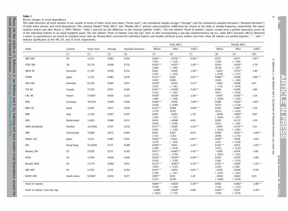
Table 1

Recent changes in serial dependence.

This table describes all stock markets in our sample in terms of index series start dates (“Series start”), the annualized sample average (“Average”) and the annualized standard deviation (“Standard deviation”)

of daily index returns, and serial dependence. The columns labeled “Daily AR(1)” and “Weekly AR(1)” present autocorrelation coefficients for returns at the daily or weekly frequency, respectively. We report

statistics before and after March 3, 1999 (“Before,” “After”) and test for the difference in the columns labeled “t (diff.).” The row labeled “Panel of indexes” reports results from a pooled regression across all

of the individual indexes in an equal-weighted panel. The row labeled “Panel of indexes (one-day lag)” does so after incorporating a one-day implementation lag [i.e., daily AR(1) becomes AR(2)]. Reported

t -values (in parentheses) are based on standard errors that are Newey-West corrected for individual indexes and double-clustered across indexes and time when all indexes are pooled together. ∗ , ∗∗ , and ∗∗∗

indicate significance at the 10%, 5%, and 1% level, respectively.

Daily AR(1) Weekly AR(1)

Index Country Series Start Average Standard deviation Before After t (diff.) Before After t (diff.)

(1) (2) (3) (4) (5) (6) (7) (8) (9) (10)

S&P 500 US 1/1/51 0.082 0.154 0.103 ∗∗∗ −0.076 ∗∗∗ −6.64 ∗∗∗ 0.037 −0.077 -2.07 ∗∗(7.45) ( −3.29) (1.28) ( −1.64)

FTSE 100 UK 2/1/78 0.048 0.176 0.053 ∗∗∗ −0.037 ∗∗ −3.43 ∗∗∗ 0.034 −0.102 ∗∗ -1.70 ∗(2.86) ( −1.99) (0.54) ( −2.07)

DJESI 50 Eurozone 1/1/87 0.050 0.214 0.041 −0.029 −2.26 ∗∗ −0.013 −0.155 ∗∗ -1.40

(1.62) ( −1.63) ( −0.14) ( −3.25)

TOPIX Japan 1/1/51 0.083 0.170 0.121 ∗∗∗ 0.016 −4.41 ∗∗∗ 0.068 ∗∗∗ −0.058 -2.86 ∗∗∗(8.10) (0.89) (2.69) ( −1.60)

ASX 200 Australia 6/1/92 0.065 0.153 0.070 ∗∗ −0.025 −2.51 ∗∗ −0.067 −0.038 0.37

(2.10) ( −1.41) ( −1.12) ( −0.78)

TSE 60 Canada 2/1/82 0.051 0.166 0.167 ∗∗∗ −0.038 ∗ −5.42 ∗∗∗ 0.046 −0.028 -1.06

(5.32) ( −1.81) (0.91) ( −0.58)

CAC 40 France 7/10/87 0.056 0.223 0.043 ∗ −0.030 ∗ −2.45 ∗∗ −0.047 −0.166 ∗∗∗ -1.34

(1.80) ( −1.68) ( −0.64) ( −3.29)

DAX Germany 10/2/59 0.049 0.196 0.066 ∗∗∗ −0.016 −3.49 ∗∗∗ 0.008 −0.102 ∗∗ -1.96 ∗∗(4.28) ( −0.90) (0.25) ( −2.24)

IBEX 35 Spain 1/6/87 0.077 0.224 0.153 ∗∗∗ 0.004 −4.64 ∗∗∗ 0.019 −0.097 ∗∗∗ -1.38

(5.79) (0.19) (0.25) ( −2.63)

MIB Italy 1/1/93 0.067 0.247 0.043 −0.023 −1.76 ∗ −0.036 −0.083 ∗∗ -0.67

(1.28) ( −1.37) ( −0.64) ( −1.97)

AEX Netherlands 1/4/83 0.088 0.212 0.014 −0.008 −0.62 0.030 −0.115 ∗ -1.29

(0.50) ( −0.36) (0.31) ( −1.90)

OMX Stockholm Sweden 12/19/86 0.118 0.232 0.117 ∗∗∗ −0.029 −4.54 ∗∗∗ −0.015 −0.135 ∗∗∗ -1.51

(4.47) ( −1.56) ( −0.23) ( −2.85)

SMI Switzerland 7/4/88 0.073 0.184 0.047 0.027 −0.55 0.050 −0.141 ∗∗∗ −2.64 ∗∗∗(1.52) (1.36) (0.98) ( −2.76)

Nikkei 225 Japan 1/2/51 0.087 0.192 0.042 ∗∗∗ −0.031 -3.03 ∗∗∗ 0.047 ∗∗ −0.018 −1.64 ∗(2.79) ( −1.65) (1.91) ( −0.58)

HSI Hong Kong 11/24/69 0.171 0.286 0.059 ∗∗∗ −0.012 −2.31 ∗∗ 0.142 ∗∗∗ −0.012 −2.65 ∗∗∗(2.80) ( −0.54) (3.03) ( −0.35)

Nasdaq 100 US 2/5/85 0.115 0.265 0.071 ∗∗ −0.065 ∗∗∗ −3.45 ∗∗∗ −0.001 −0.074 −1.06

(2.23) ( −2.79) ( −0.02) ( −1.63)

NYSE US 1/3/66 0.036 0.160 0.145 ∗∗∗ −0.059 ∗∗ −6.96 ∗∗∗ 0.039 −0.079 −1.86 ∗(8.39) ( −2.50) (1.06) ( −1.52)

Russell 20 0 0 US 1/1/79 0.066 0.191 0.273 ∗∗∗ −0.062 ∗∗ −6.33 ∗∗∗ 0.192 ∗∗∗ −0.065 −3.25 ∗∗∗(5.83) ( −2.52) (2.92) (-1.48)

S&P 400 US 1/1/91 0.110 0.194 0.147 ∗∗∗ −0.033 −5.01 ∗∗∗ −0.001 −0.064 −0.78

(5.38) ( −1.41) ( −0.01) ( −1.25)

KOSPI 200 South Korea 9/10/87 0.034 0.277 0.057 ∗∗ 0.011 −1.47 −0.042 −0.024 0.25

(2.32) (0.58) ( −0.68) ( −0.59)

Panel of indexes 0.094 ∗∗∗ −0.026 ∗ −5.30 ∗∗∗ 0.042 −0.082 ∗∗ −2.86 ∗∗∗(5.58) ( −1.94) (1.54) ( −2.32)

Panel of indexes (one-day lag) −0.009 −0.029 ∗ −0.88 0.065 ∗∗∗ −0.021 −2.43 ∗∗( −0.62) ( −1.78) (3.06) ( −0.74)

Ple

ase

cite th

is a

rticle a

s: G

. B

altu

ssen

, S

. v

an B

ek

ku

m a

nd Z

. D

a, In

de

xin

g a

nd sto

ck m

ark

et se

rial d

ep

en

de

nce

aro

un

d th

e

wo

rld, Jo

urn

al o

f F

ina

ncia

l E

con

om

ics, h

ttps://d

oi.o

rg/1

0.1

01

6/j.jfi

ne

co.2

01

8.0

7.01

6

G. Baltussen, S. van Bekkum and Z. Da / Journal of Financial Economics xxx (xxxx) xxx 7

ARTICLE IN PRESS

JID: FINEC [m3Gdc; December 14, 2018;13:23 ]

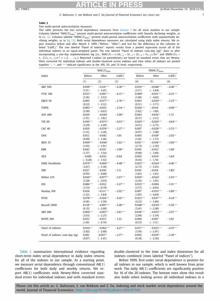
Table 2

Two multi-period autocorrelation measures.

This table presents the two serial dependence measures from Section 3 for all stock markets in our sample.

Columns labeled “MAC(5) index ” present multi-period autocorrelation coefficients with linearly declining weights, as

in Eq. (2) . Columns labeled “EMAC(5) index ” present multi-period autocorrelation coefficients with exponentially de-

clining weights, as in Eq. (3) . Both serial dependence measures are calculated using daily index returns. We re-

port statistics before and after March 3, 1999 (“Before,” “After”) and test for the difference in the columns la-

beled “t (diff.).” The row labeled “Panel of indexes” reports results from a pooled regression across all of the

individual indexes in an equal-weighted panel. The row labeled “Panel of indexes (one-day lag)” does so after

incorporating a one-day implementation lag [i.e., MAC (5) = r t (4 r t−2 + 3 r t−3 + 2 r t−4 + 1 r t−5 ) / 5 σ 2 and EMAC (5) t =

r t · f (λ5 , r t−τ ) /σ 2 , τ = 2 , . . . , ∞ , ]. Reported t -values (in parentheses) are based on standard errors that are Newey-

West corrected for individual indexes and double-clustered across indexes and time when all indexes are pooled

together. ∗ , ∗∗ , and ∗∗∗ indicate significance at the 10%, 5%, and 1% level, respectively.

MAC(5) index EMAC(5) index

Index Before After t (diff.) Before After t (diff.)

(1) (2) (3) (4) (5) (6)

S&P 500 0.050 ∗∗∗ −0.141 ∗∗∗ −4.30 ∗∗∗ 0.014 ∗∗∗ −0.048 ∗∗∗ −4.46 ∗∗∗

(3.11) ( −3.41) (3.17) ( −3.64)

FTSE 100 0.031 ∗∗ −0.091 ∗∗∗ −4.13 ∗∗∗ 0.009 ∗ −0.031 ∗∗∗ −4.25 ∗∗∗

(2.18) ( −3.52) (1.68) ( −4.02)

DJESI 50 0.003 −0.077 ∗∗∗ −2.76 ∗∗∗ 0.003 −0.029 ∗∗∗ −3.25 ∗∗∗

(0.22) ( −3.12) (0.51) ( −3.71)

TOPIX 0.082 ∗∗∗ −0.025 −2.54 ∗∗∗ 0.026 ∗∗∗ −0.014 −4.90 ∗∗∗

(5.99) ( −0.63) (5.82) ( −1.09)

ASX 200 0.029 −0.044 ∗ −2.09 ∗∗ 0.003 −0.016 ∗∗ −1.72

(1.15) ( −1.82) (0.37) ( −2.13)

TSE 60 0.100 ∗∗∗ −0.075 ∗∗ −4.93 ∗∗∗ 0.029 ∗∗∗ −0.029 ∗∗∗ −4.64 ∗∗∗

(5.29) ( −2.49) (4.51) ( −2.72)

CAC 40 0.020 −0.074 ∗∗∗ −3.27 ∗∗∗ 0.007 −0.028 ∗∗∗ −3.53 ∗∗∗

(1.13) ( −3.26) (0.97) ( −3.98)

DAX 0.012 −0.042 −1.65 0.005 −0.018 ∗ −2.02 ∗∗

(0.99) ( −1.38) (1.10) ( −1.73)

IBEX 35 0.099 ∗∗∗ −0.044 ∗ −3.62 ∗∗∗ 0.031 ∗∗∗ −0.018 ∗∗∗ −3.66 ∗∗∗

(3.10) ( −1.91) (2.75) ( −2.50)

MIB 0.043 −0.031 −1.98 ∗∗ 0.010 −0.012 ∗ −1.68 ∗

(1.37) ( −1.54) (0.90) ( −1.68)

AEX −0.005 −0.033 −0.94 0.003 −0.014 ∗ −1.64 ∗

( −0.28) ( −1.32) (0.43) ( −1.74)

OMX Stockholm 0.079 ∗∗∗ −0.066 ∗∗∗ −4.48 ∗∗∗ 0.025 ∗∗∗ −0.024 ∗∗∗ −4.46 ∗∗∗

(3.07) ( −3.36) (2.73) ( −3.93)

SMI 0.027 −0.016 −1.11 0.010 −0.014 −1.89 ∗

(0.95) ( −0.60) (1.05) ( −1.65)

Nikkei 225 0.030 ∗∗ −0.077 ∗∗ −2.67 ∗∗∗ 0.010 ∗∗ −0.024 ∗ −2.63 ∗∗∗

(2.28) ( −2.03) (2.43) ( −1.95)

HSI 0.086 ∗∗∗ −0.012 −3.27 ∗∗∗ 0.033 ∗∗∗ −0.004 −3.51 ∗∗∗

(3.33) ( −0.78) (3.57) ( −0.83)

Nasdaq 100 0.026 −0.111 ∗∗∗ −3.92 ∗∗∗ 0.007 −0.035 ∗∗∗ −3.80 ∗∗∗

(1.32) ( −3.84) (1.05) ( −4.04)

NYSE 0.078 ∗∗∗ −0.104 ∗∗∗ −4.10 ∗∗∗ 0.022 ∗∗∗ −0.037 ∗∗∗ −4.24 ∗∗∗

(4.18) ( −2.59) (4.22) ( −2.89)

Russell 20 0 0 0.138 ∗∗∗ −0.097 ∗∗∗ −5.46 ∗∗∗ 0.048 ∗∗∗ −0.034 ∗∗∗ −5.56 ∗∗∗

(6.35) ( −2.60) (5.41) ( −2.90)

S&P 400 0.066 ∗∗∗ −0.067 ∗∗ −3.81 ∗∗∗ 0.018 ∗∗∗ −0.025 ∗∗∗ −3.67 ∗∗∗

(3.63) ( −2.25) (2.84) ( −2.54)

KOSPI 200 0.033 −0.013 −1.32 0.006 −0.007 −1.02

(1.10) ( −0.74) (0.55) ( −1.11)

Panel of indexes 0.054 ∗∗∗ −0.062 ∗∗∗ −4.27 ∗∗∗ 0.017 ∗∗∗ −0.023 ∗∗∗ −4.35 ∗∗∗

(3.82) ( −2.68) (3.56) ( −2.91)

Panel of indexes (one-day lag) 0.001 -0.057 ∗∗ −2.17 ∗∗ 0.002 −0.019 ∗∗ −2.39 ∗∗

(0.07) ( −2.41) (0.38) ( −2.50)

Table 1 summarizes international evidence regarding

short-term index serial dependence in daily index returns

for all of the indexes in our sample. As a starting point,

we measure serial dependence through conventional AR(1)

coefficients for both daily and weekly returns. We re-

port AR(1) coefficients with Newey-West corrected stan-

dard errors for individual indexes and with standard errors

Please cite this article as: G. Baltussen, S. van Bekkum and Z. Da

world, Journal of Financial Economics, https://doi.org/10.1016/j.jfi

double-clustered in the time and index dimension for all

indexes combined (rows labeled “Panel of indices”).

Before 1999, first-order serial dependence is positive for

all indexes in our sample, which is well known from prior

work. The daily AR(1) coefficients are significantly positive

for 16 of the 20 indexes. The bottom rows show this result

also holds when looking across all individual indexes in a

, Indexing and stock market serial dependence around the

neco.2018.07.016

8 G. Baltussen, S. van Bekkum and Z. Da / Journal of Financial Economics xxx (xxxx) xxx

ARTICLE IN PRESS

JID: FINEC [m3Gdc; December 14, 2018;13:23 ]

3 Variance differences and variance ratios are central statistics in the

literature on serial dependence. See Campbell et al. (1997) (1997; Chapter

3) for an introduction of the key concepts, and O’Hara and Ye (2011) and

Ben-David et al. (2018) for recent use.

panel setup. Serial dependence becomes indistinguishable

from zero when using a one-day implementation lag, to

mitigate the impact of nonsynchronous trading and other

microstructure biases ( Jegadeesh, 1990 ).

In stark contrast, first-order daily autocorrelation turns

negative for 16 out of 20 indexes in the post-1999 sub-

sample. The coefficients are significantly negative for seven

of 20 indexes and for the panel of indexes both with and

without the one-day implementation lag. Column 3 labeled

“t (diff.)” shows that the decline in AR(1) coefficients be-

tween the two subsamples is significant in 17 of the 20

indexes and across the cross section of indexes (without

implementation lag).

The decline in serial dependence is not limited to daily,

or first-order, autocorrelations. We observe a similarly de-

clining trend in serial dependence at the weekly frequency,

with weekly AR(1) coefficients in Table 1 turning negative

for all 20 indexes in the post-1999 subsample. Moreover,

weekly AR(1) coefficients decline between the two sub-

samples for 18 of the 20 indexes and nine such declines

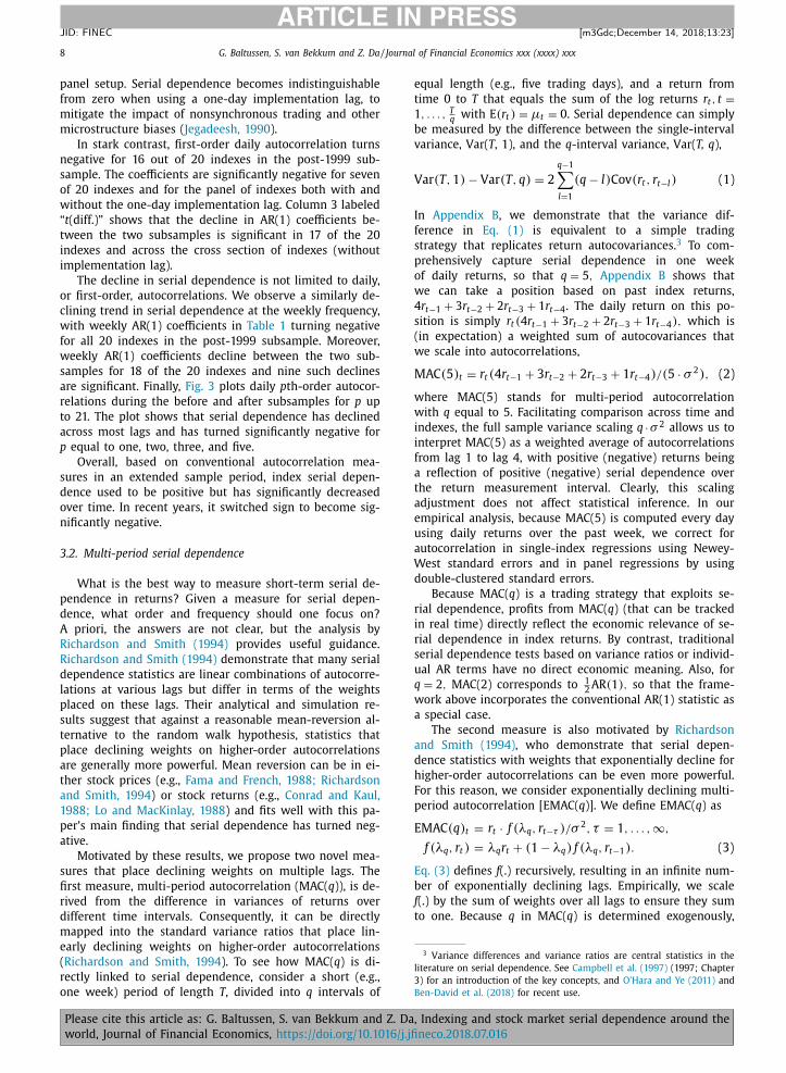
are significant. Finally, Fig. 3 plots daily p th-order autocor-

relations during the before and after subsamples for p up

to 21. The plot shows that serial dependence has declined

across most lags and has turned significantly negative for

p equal to one, two, three, and five.

Overall, based on conventional autocorrelation mea-

sures in an extended sample period, index serial depen-

dence used to be positive but has significantly decreased

over time. In recent years, it switched sign to become sig-

nificantly negative.

3.2. Multi-period serial dependence

What is the best way to measure short-term serial de-

pendence in returns? Given a measure for serial depen-

dence, what order and frequency should one focus on?

A priori, the answers are not clear, but the analysis by

Richardson and Smith (1994) provides useful guidance.

Richardson and Smith (1994) demonstrate that many serial

dependence statistics are linear combinations of autocorre-

lations at various lags but differ in terms of the weights

placed on these lags. Their analytical and simulation re-

sults suggest that against a reasonable mean-reversion al-

ternative to the random walk hypothesis, statistics that

place declining weights on higher-order autocorrelations

are generally more powerful. Mean reversion can be in ei-

ther stock prices (e.g., Fama and French, 1988; Richardson

and Smith, 1994 ) or stock returns (e.g., Conrad and Kaul,

1988; Lo and MacKinlay, 1988 ) and fits well with this pa-

per’s main finding that serial dependence has turned neg-

ative.

Motivated by these results, we propose two novel mea-

sures that place declining weights on multiple lags. The

first measure, multi-period autocorrelation (MAC( q )), is de-

rived from the difference in variances of returns over

different time intervals. Consequently, it can be directly

mapped into the standard variance ratios that place lin-

early declining weights on higher-order autocorrelations

( Richardson and Smith, 1994 ). To see how MAC( q ) is di-

rectly linked to serial dependence, consider a short (e.g.,

one week) period of length T , divided into q intervals of

Please cite this article as: G. Baltussen, S. van Bekkum and Z. Da

world, Journal of Financial Economics, https://doi.org/10.1016/j.jfi

equal length (e.g., five trading days), and a return from

time 0 to T that equals the sum of the log returns r t , t =1 , . . . , T q with E(r t ) = μt = 0 . Serial dependence can simply

be measured by the difference between the single-interval

variance, Var( T , 1), and the q -interval variance, Var( T, q ),

Var (T , 1) − Var (T , q ) = 2

q −1 ∑

l=1

(q − l) Cov (r t , r t−l ) (1)

In Appendix B , we demonstrate that the variance dif-

ference in Eq. (1) is equivalent to a simple trading

strategy that replicates return autocovariances. 3 To com-

prehensively capture serial dependence in one week

of daily returns, so that q = 5 , Appendix B shows that

we can take a position based on past index returns,

4 r t−1 + 3 r t−2 + 2 r t−3 + 1 r t−4 . The daily return on this po-

sition is simply r t (4 r t−1 + 3 r t−2 + 2 r t−3 + 1 r t−4 ) , which is

(in expectation) a weighted sum of autocovariances that

we scale into autocorrelations,

MAC (5) t = r t (4 r t−1 + 3 r t−2 + 2 r t−3 + 1 r t−4 ) / (5 · σ 2 ) , (2)

where MAC(5) stands for multi-period autocorrelation

with q equal to 5. Facilitating comparison across time and

indexes, the full sample variance scaling q ·σ 2 allows us to

interpret MAC(5) as a weighted average of autocorrelations

from lag 1 to lag 4, with positive (negative) returns being

a reflection of positive (negative) serial dependence over

the return measurement interval. Clearly, this scaling

adjustment does not affect statistical inference. In our

empirical analysis, because MAC(5) is computed every day

using daily returns over the past week, we correct for

autocorrelation in single-index regressions using Newey-

West standard errors and in panel regressions by using

double-clustered standard errors.

Because MAC( q ) is a trading strategy that exploits se-

rial dependence, profits from MAC( q ) (that can be tracked

in real time) directly reflect the economic relevance of se-

rial dependence in index returns. By contrast, traditional

serial dependence tests based on variance ratios or individ-

ual AR terms have no direct economic meaning. Also, for

q = 2 , MAC(2) corresponds to 1 2 AR (1) , so that the frame-

work above incorporates the conventional AR(1) statistic as

a special case.

The second measure is also motivated by Richardson

and Smith (1994) , who demonstrate that serial depen-

dence statistics with weights that exponentially decline for

higher-order autocorrelations can be even more powerful.

For this reason, we consider exponentially declining multi-

period autocorrelation [EMAC( q )]. We define EMAC( q ) as

EMAC (q ) t = r t · f (λq , r t−τ ) /σ 2 , τ = 1 , . . . , ∞ ,

f (λq , r t ) = λq r t + (1 − λq ) f (λq , r t−1 ) . (3)

Eq. (3) defines f (.) recursively, resulting in an infinite num-

ber of exponentially declining lags. Empirically, we scale

f (.) by the sum of weights over all lags to ensure they sum

to one. Because q in MAC( q ) is determined exogenously,

, Indexing and stock market serial dependence around the

neco.2018.07.016

G. Baltussen, S. van Bekkum and Z. Da / Journal of Financial Economics xxx (xxxx) xxx 9

ARTICLE IN PRESS

JID: FINEC [m3Gdc; December 14, 2018;13:23 ]

Fig. 3. Recent changes in serial dependence for different lag orders. This figure plots autocorrelation coefficients for our panel of stock market indexes

across the world, for different lag orders ( p ) before and after March 3, 1999. We repeat the analysis in the penultimate row of Table 1 at the daily frequency,

and calculate daily autocorrelations separately for lag order 1 (i.e., 1 day) to 21 (i.e., 1 month). The ranges centered around each AR( p ) coefficient represent

its corresponding 90% confidence interval.

we compare the MAC( q ) and EMAC( q ) measures using the

parameter λq , which is chosen such that the half-life of

EMAC( q ) (the period over which 50% of all weights are dis-

tributed) is equal to the half-life of MAC( q ).

Table 2 confirms the dramatic decline in serial depen-

dence using both MAC(5) and EMAC(5). Average MAC(5)

before 1999 is positive for 19 out of the 20 indexes and

significantly so for 11 of them. By contrast, MAC(5) after

1999 is negative for all indexes and significantly so for 13

Please cite this article as: G. Baltussen, S. van Bekkum and Z. Da

world, Journal of Financial Economics, https://doi.org/10.1016/j.jfi

of the 20 indexes. The change in MAC(5) is significant in

16 of the 20 indexes.

We find virtually identical results when comparing

EMAC(5) with MAC(5), indicating that the assigned weights

in MAC(5) are very close to the optimal weights in

EMAC(5) and that MAC(5) efficiently combines autocorre-

lations at multiple lags. Hence, we focus on MAC(5) when

presenting results in the remainder of the paper, given that

it maps into the familiar variance ratio tests and also has

, Indexing and stock market serial dependence around the

neco.2018.07.016

10 G. Baltussen, S. van Bekkum and Z. Da / Journal of Financial Economics xxx (xxxx) xxx

ARTICLE IN PRESS

JID: FINEC [m3Gdc; December 14, 2018;13:23 ]

a convenient trading strategy interpretation. In the Online

Appendix, we further demonstrate the similarity of our re-

sults when using either MAC( q ) or EMAC( q ) definitions and

for lag orders varying from one day up to one month of re-

turns (i.e., q = 2 up to q = 22 ).

4. Serial dependence and indexing

In this section, we use MAC(5) to further analyze how

serial dependence in index returns varies over time and

in the cross section. We present evidence that the large

negative changes in index serial dependence are associ-

ated with the increased popularity of index products. In-

dex MAC(5) is positive up to the introduction of the fu-

tures and becomes significantly negative thereafter. This

pattern can be found in nearly all indexes in our sample

even though their futures are introduced over a time span

of almost two decades. MAC(5) is also significantly nega-

tive in futures returns and ETFs returns since the introduc-

tion of futures and ETFs, respectively. We use the percent-

age of assets allocated to index products as a measure for

the extent of indexing and find a significantly negative re-

lation with serial dependence in both the time series and

the cross section.

4.1. Serial dependence and futures introductions

Figs. 1 and 2 show that index serial dependence be-

came negative as index products increased in popularity

around the world. However, the correlation between index-

ing and negative serial dependence could simply reflect a

common time trend. An important advantage of our study

is its broad coverage of 20 major market indexes. Consider-

able cross-market variation exists in the starting date of in-

dexing. The cross-sectional dimension helps to isolate the

link between indexing and index serial dependence.

We first determine the break date at which each index’s

serial dependence changes the most using a purely statisti-

cal, data-driven approach. For each index, we run cumula-

tive sum (CUSUM) break tests and retrieve the break date

from the data as the date at which the cumulative sum of

standardized deviations from average MAC(5) is the largest.

We ignore any breaks in October 1987 and September

2008, which are characterized by extreme market turmoil,

and report results in the first column of Table 3 . Remov-

ing these two extreme episodes from other parts of our

empirical tests does not alter our results in any significant

way. The asterisks indicate that the change in MAC(5) Index

around the break date is significant for 15 out of the 20

indexes. A large variation exists in the break dates across

the 20 indexes.

We next examine whether the variation in break dates

can be explained by the variation in the starting date of

indexing. Although the first index fund has been around

since December 31, 1975, a long time passed before index

funds became popular. 4 Thus, we regard the introduction

4 For instance, John C. Bogle, founder of Vanguard, recounts that the

road to success was long and winding for the company: “[I]n the early

days, the idea that managers of passive equity funds could out-pace the

returns earned by active equity managers as a group was derogated and

Please cite this article as: G. Baltussen, S. van Bekkum and Z. Da

world, Journal of Financial Economics, https://doi.org/10.1016/j.jfi

of futures contracts as the start of indexing and report the

futures introduction dates in the second column of Table 3 .

Comparing the break dates with futures introduction dates,

a structural break in serial dependence generally happens

just a few years after index futures are introduced. Break

dates that occur before or many years after the futures in-

troduction tend to indicate insignificant breaks. A regres-

sion of break dates on futures introduction dates produces

a positive and highly significant slope coefficient ( t -value =

3.17) and an R-squared of 0.36. We present this regression

including the raw data in Panel A of Fig. 4 .

Panel B presents additional evidence by plotting cumu-

lative MAC(5) (i.e., cumulative serial dependence trading

profits) across all equity indexes, futures, and ETFs over

our sample period. The horizontal axis is in event time and

plots the years between the calendar date and the futures

introduction date [for index MAC(5) and futures MAC(5)]

or the ETF introduction date [for ETF MAC(5)]. Cumulative

serial dependence in index returns clearly has an inverse

U-shape that centers around the various futures introduc-

tions. Cumulative index MAC(5) is increasing in the years

prior to the 20 futures introductions, indicating positive se-

rial dependence. After the introduction, cumulative index

MAC(5) decreases, indicating negative serial dependence.

The tipping point across all indexes lies within five years

after the futures introductions.

In Columns 3 and 4 of Table 3 , we directly estimate

the impact of futures introductions on serial dependence

by regressing index MAC(5) on a dummy variable, D intro ,

that is equal to one if at least one equity futures contract

is introduced on the respective index and zero otherwise,

MAC (5) Index,t = b 1 + b 2 · D intro,t + ε t , (4)

for each of the 20 indexes. When examining individual in-

dexes, Eq. (4) is a time series regression with Newey-West–

corrected standard errors. When examining the pooled

sample of indexes, Eq. (4) is a panel regression with

standard errors double-clustered (across indexes and over

time).

Table 3 reports these results along with simple averages

for MAC(5) futures and MAC(5) ETF (for which D intro is always

equal to one). The intercept term b 1 is positive for 17 in-

dexes and significant for 11 of them, suggesting positive

serial dependence before the futures introduction consis-

tent with the papers that examine periods up to the 1990s.

The dummy coefficient b 2 measures the change in serial

dependence after the futures introduction, which is neg-

ative for all 20 indexes with 15 of them significant. The

sum of both coefficients ( b 1 + b 2 ) measures index MAC(5)

after the futures introduction, which is negative for 17 out

of the 20 indexes and significant for nine. Because futures

introductions occur between 1982 and 20 0 0, these find-

ings are unlikely to be driven by a single event. In addi-

tion, index products experience negative serial dependence

right away, from the moment they are introduced. Average

MAC(5) futures is negative for each of the 20 indexes and sig-

nificant for 12 of them. Similarly, MAC(5) ETF is negative for

ridiculed. (The index fund was referred to as Bogle’ s Folly.)” ( Bogle, 2014

p. 46).

, Indexing and stock market serial dependence around the

neco.2018.07.016

G. Baltussen, S. van Bekkum and Z. Da / Journal of Financial Economics xxx (xxxx) xxx 11

ARTICLE IN PRESS

JID: FINEC [m3Gdc; December 14, 2018;13:23 ]

Table 3

Breaks in serial dependence.

This table presents results on structural breaks in serial dependence for all stock markets in our sample. Endogenously determined structural

break dates in index MAC(5) (“MAC(5) Index break date”) are based on the maximum cumulative sum (CUSUM) of deviations from each index’s

average MAC(5) after excluding October 1987 and the 2008 financial crisis. Asterisks in this column indicate significance of a test against the

null hypothesis that the break around the break date results from a Brownian motion. We also report the date at which the first corresponding

index futures started trading (“Futures start date”). The columns labeled “MAC (5) Index = b 1 + b 2 · D intro ” show the results of regressing daily returns

on index MAC(5) against the intercept and a futures introduction dummy that equals one after the futures introduction date and zero otherwise

(coefficients b 1 and b 2 are reported in percentages). Average futures MAC(5) (“MAC(5) futures ”) and average Exchange Traded Fund (ETF) MAC(5)

(“MAC(5) ETF ”; with corresponding ETF introduction dates) are calculated since the futures or ETF introduction date, respectively. The row labeled

“Panel of indexes” reports results from a pooled regression across all of the individual indexes in an equal-weighted panel. The last row [“Panel of

indexes (1-day lag)”] applies a one-day implementation lag between current and past returns [i.e., MAC (5) = r t (4 r t−2 + 3 r t−3 + 2 r t−4 + 1 r t−5 ) / 5 σ 2 ].

Reported t -values (in parentheses) are based on standard errors that are Newey-West corrected for individual indexes and double-clustered across

indexes and time when all indexes are pooled together. ∗ , ∗∗ , and ∗∗∗ indicate significance at the 10%, 5%, and 1% level, respectively.

MAC(5) index Futures MAC(5 ) Index = b 1 + b 2 · D intro MAC(5) futures MAC(5) ETF

break date start date b 1 b 2 Average Start date Average

(1) (2) (3) (4) (5) (6) (7)

S&P 500 8/14/87 ∗∗∗ 4/22/82 0.085 ∗∗∗ −0.165 ∗∗∗ −0.091 ∗∗ 01-29-93 −0.087 ∗∗∗

(7.12) ( −5.25) ( −2.49) ( −3.49)

FTSE 100 9/2/98 ∗∗∗ 5/3/84 −0.008 −0.021 −0.043 ∗∗∗ 04-28-00 −0.109 ∗∗∗

( −1.35) ( −1.17) ( −2.67) ( −3.18)

DJESI 50 1/7/00 6/22/98 −0.001 −0.070 ∗∗ −0.070 ∗∗∗ 03 −21-01 −0.065 ∗∗∗

( −0.08) ( −2.51) ( −3.67) ( −3.30)

TOPIX 11/30/93 ∗∗∗ 9/5/88 0.090 ∗∗∗ −0.086 ∗∗∗ −0.049 ∗∗∗ 07-13 −01 -0.032

(6.38) ( −2.67) ( −2.61) ( −1.25)

ASX 200 10/29/97 5/3/00 0.017 −0.061 ∗ −0.036 08-27 −01 -0.055 ∗∗

(0.76) ( −1.78) ( −1.54) ( −2.26)

TSE 60 4/17/00 ∗∗∗ 9/7/99 0.098 ∗∗∗ -0.177 ∗∗∗ −0.061 ∗∗∗ 10-04-99 -0.047 ∗∗

(5.33) ( −4.92) ( −2.84) ( −2.06)

CAC 40 3/07/00 ∗ 12/8/88 0.071 −0.113 −0.049 ∗∗∗ 01-22 −01 −0.062 ∗∗∗

(0.77) ( −1.21) ( −3.23) ( −2.81)

DAX 1/29/87 11/23/90 0.022 −0.058 ∗∗ −0.021 01-03-01 −0.020

(1.58) ( −2.20) ( −1.18) ( −0.90)

IBEX 35 9/2/98 ∗∗∗ 4/20/92 0.151 ∗∗ −0.167 ∗∗ -0.036 ∗∗ 10-03-06 −0.034

(2.38) ( −2.52) ( −2.10) ( −1.31)

MIB 9/24/01 11/28/94 0.110 ∗ −0.133 ∗∗ −0.017 11-12-03 −0.014

(1.94) ( −2.24) ( −1.00) ( −0.60)

AEX 5/26/86 10/26/88 −0.012 −0.009 −0.028 11-21-05 −0.036

( −0.33) ( −0.24) ( −1.59) ( −1.36)

OMX Stockholm 4/6/00 ∗∗∗ 1/2/90 0.073 −0.090 ∗ −0.059 ∗∗∗ 04-24-01 −0.079 ∗∗∗

(1.56) ( −1.80) ( −3.82) ( −3.15)

SMI 3/24/03 11/9/90 0.008 −0.009 −0.012 03-15-01 −0.036

(0.12) ( −0.13) ( −0.62) ( −1.46)

Nikkei 225 10/2/90 ∗∗∗ 9/5/88 0.058 ∗∗∗ −0.132 ∗∗∗ −0.055 ∗∗∗ 07-13-01 −0.050 ∗

(4.30) ( −4.31) ( −2.88) ( −1.92)

HSI 12/25/87 ∗∗ 5/6/86 0.137 ∗∗∗ −0.135 ∗∗∗ −0.015 11-12-99 −0.039 ∗

(3.56) ( −3.25) ( −0.52) ( −1.88)

Nasdaq 100 9/1/98 ∗∗ 4/11/96 0.043 ∗∗ −0.143 ∗∗∗ −0.073 ∗∗∗ 03-10-99 −0.077 ∗∗∗

(2.09) ( −4.36) ( −3.28) ( −3.29)

NYSE 8/14/87 ∗∗∗ 5/6/82 0.138 ∗∗∗ −0.182 ∗∗∗ −0.100 04-02-04 −0.069 ∗

(7.77) ( −5.77) ( −2.43) ( −1.91)

Russell 20 0 0 4/17/00 ∗∗∗ 2/4/93 0.155 ∗∗∗ −0.202 ∗∗∗ −0.049 ∗∗ 05-26-00 −0.064 ∗∗∗

(5.53) ( −5.02) ( −2.22) ( −2.77)

S&P 400 1/15/99 ∗∗ 2/14/92 0.141 ∗∗∗ −0.173 ∗∗∗ −0.048 ∗∗ 05-26-00 −0.041

(2.79) ( −3.15) ( −2.01) ( −1.63)

KOSPI 200 11/17/99 5/3/96 0.007 −0.002 −0.018 10-14-02 −0.024

(0.34) ( −0.08) ( −0.96) ( −1.00)

Panel of indexes 0.072 ∗∗∗ −0.108 ∗∗∗ −0.047 ∗∗∗ −0.054 ∗∗∗

(4.55) ( −5.01) ( −3.16) ( −2.94)

Panel of indexes (one-day lag) 0.018 -0.065 ∗∗∗ −0.044 ∗∗∗ −0.046 ∗∗

(1.41) ( −3.41) ( −2.87) ( −2.42)

all indexes and significantly so for 12 of them, with values

slightly more negative than for MAC(5) futures .

In the bottom rows of Table 3 , we run a panel re-

gression across all markets of either the MAC(5) Index ,

MAC(5) futures , or MAC(5) ETF series, with standard errors

clustered at the time and index level as in Table 3 . Global

MAC(5) is significantly positive prior to the futures in-

Index

Please cite this article as: G. Baltussen, S. van Bekkum and Z. Da

world, Journal of Financial Economics, https://doi.org/10.1016/j.jfi

troduction (0.072 with t -value = 4.55) and reduces sub-

stantially and significantly after the introduction ( −0.108

with t -value = −5.01) to a significantly negative −0.036 ( t -

value = −2.11). Similarly, the coefficients on MAC(5) futures

and MAC(5) ETF are significantly negative when pooled to-

gether across indexes. In unreported results, we re-run

Eq. (4) after creating separate dummy variables for fu-

, Indexing and stock market serial dependence around the

neco.2018.07.016

12 G. Baltussen, S. van Bekkum and Z. Da / Journal of Financial Economics xxx (xxxx) xxx

ARTICLE IN PRESS

JID: FINEC [m3Gdc; December 14, 2018;13:23 ]

Fig. 4. Serial dependence and the start of indexing. This figure plots serial dependence dynamics against the start of indexing in calendar time (Panel A)

and in event time (Panel B). For each index, indexing starts on the day that the first corresponding equity index futures contract was introduced. Panel

A plots endogenously determined break points in serial dependence against the start of indexing. The fitted line is based on a linear regression of the

MAC(5) break date on the indexing start date. Panel B plots cumulative index MAC(5) (normalized to start at one) around the start of indexing for all

indexes combined. The horizontal axis reflects event time, with t = 0 reflecting the indexing start date. The black line plots (equally weighted) cumulative

index MAC(5), and the gray solid line and gray dashed line plot cumulative futures MAC(5) and exchange-traded fund (ETF) MAC(5), respectively.

tures introductions and ETF introductions. Coefficients on

these variables are −0.060 and −0.080 ( t -value = −3.86

and −2.91), respectively. 5

5 Also, Etula et al. (2015) argue that month-end liquidity needs of in-

vestors can lead to structural and correlated buying and selling pressures

of investors around month-ends, thereby causing short-term reversals in

equity indexes. We verify that the above results are robust to these pat-

terns. When we include separate dummy variables for the three periods

Please cite this article as: G. Baltussen, S. van Bekkum and Z. Da

world, Journal of Financial Economics, https://doi.org/10.1016/j.jfi

The MAC( q ) measure is estimated from a trading strat-

egy that can be executed in real time. The trading

strategy allows us to demonstrate that negative serial

around month-ends most likely subject to buying and selling pressures

(i.e., t -8 to t -4, t -3 to t , and t +1 to t +3) and their interaction with the

futures introduction dates of each market, we find coefficients of 0.071

( t -value = 4.29) on the intercept and -0.107 ( t -value = -4.87) on the fu-

tures introduction dummy.

, Indexing and stock market serial dependence around the

neco.2018.07.016

G. Baltussen, S. van Bekkum and Z. Da / Journal of Financial Economics xxx (xxxx) xxx 13

ARTICLE IN PRESS

JID: FINEC [m3Gdc; December 14, 2018;13:23 ]

6 To examine indexing in the broadest sense, we also consider index-

ing by index mutual funds that seek to fully replicate the S&P 500 using

the CRSP Survivorship-Bias-Free US Mutual Funds Database (which cov-

ers only the US). To focus strictly on index funds, we ignore all funds

that track substantially more or less stocks than all five hundred index

constituents. The coefficient on total indexing continues to be significant

when we measure indexing by the combined assets in futures, ETFs, and

index mutual funds.

dependence in index returns is economically important.

For instance, a strategy that trades against the negative

MAC(5) using all indexes (the S&P 500 alone) in our sam-

ple would result in an annualized Sharpe ratio of 0.63

(0.67) after March 2, 1999. Similar Sharpe ratios are ob-

served for the indexes and ETFs. These Sharpe ratios com-

pare favorably against the average Sharpe ratio across the

stock markets in our sample of 0.36 and highlight the

economic importance of negative index serial dependence.

At the same time, trading against negative serial depen-

dence requires frequent rebalancing. As a result, the strat-

egy might not be exploitable to many investors after ac-

counting for transaction costs.

In sum, the introduction of indexing correlates nega-

tively with index serial dependence. We observe positive

serial dependence up to the introduction of index prod-

ucts, but economically strong and significantly negative se-

rial dependence in index and index product returns there-

after.

4.2. Serial dependence and the extent of indexing

Thus far, we have used cross-market variation in the in-

troduction of the futures contracts, which is measured by

a dummy variable. Next, we examine the relation between

serial dependence and several continuous measures of in-

dexing based on the assets allocated to index products as a

percentage of the underlying index’s market capitalization.

To measure indexing in futures, we multiply the futures

open interest (in contracts) with contract size and underly-

ing index price. To mitigate the impact of spikes in futures

open interest around roll dates, we average this measure

using a three-month moving window that corresponds to

the maturity cycle of most futures contracts. To measure

ETF indexing, we take the size of the ETF market listed on

an index (market capitalization). Both the futures measure

and the ETF measure are scaled by daily market capital-

ization of the underlying index. To measure total indexing,

we take the sum of both measures. We exclude the Russell

20 0 0, S&P 40 0, and NASDAQ indexes because open inter-

est data on the futures from either Bloomberg or Datas-

tream are available only four to ten years after the futures

introduction (this does not affect our results). Panel B of

Fig. 2 shows that the past 30 years have seen a substan-

tial rise in indexing globally, which coincides with declin-

ing serial dependence in the index.

More formally, we regress each index i ’s MAC(5) on the

extent of indexing,

MAC (5) index,it = b 1 + b 2 · Indexing it−1 + θ ′ X it−1 + ε it , (5)

where the vector X it contains the TED spread and each in-

dex’s market volatility, past market returns, and detrended

market volume as control variables in the spirit of Nagel

(2012) , Hameed et al. (2010) , and Campbell et al. (1993) ,

respectively. More details on these variables’ definitions

can be found in Appendix A . We measure indexing over

the previous day, but results are practically identical when

indexing is measured at time t or t − 5 . Table 4 presents

results of a panel regression indicating a significantly neg-

ative relation between index serial dependence and index-

ing. The coefficient of −3.131 with a t -value of −2.90 im-

Please cite this article as: G. Baltussen, S. van Bekkum and Z. Da

world, Journal of Financial Economics, https://doi.org/10.1016/j.jfi

plies that every 1% increase in indexing decreases serial

dependence by about 0.031. In fact, the point at which se-

rial dependence equals zero can be computed for the re-

gressions MAC (5) index = b 1 + b 2 · Indexing + ε as the level

of indexing at which the regression line crosses the ver-

tical axis [i.e., MAC (5) index = 0 ]. Globally, this point lies at

1.4% of index capitalization as shown in the the row la-

beled “Zero serial dependence point.”

The effect is similar when we include index fixed ef-

fects to control for unobserved differences in indexing be-

tween stock markets. The coefficient on indexing remains

of very similar size and significance at the 5% level once

we include the controls. Coefficients on detrended volume

and last month’s index volatility are unreported, but they

are in line with those in Campbell et al. (1993) and Nagel

(2012) . When separating futures indexing from ETF in-

dexing, the coefficient on futures indexing becomes larger

( −3.617) and remains significant at the 5% level, and the

coefficient on ETF indexing becomes larger ( −5.283) but

with a smaller t -value of −1.76. 6

To remove any index-specific time trend, we reestimate

Eq. (5) in differenced form,

�MAC (5) index,it = b 1 + b 2 · �Indexing it−1 + θ ′ �X it−1 + ε it ,

(6)

where differences are calculated over a three-month inter-

val to correspond with the futures rolling cycle. Columns

6–8 of Table 4 indicate that the relation between changes

in indexing and changes in index MAC(5) becomes more

significant, both economically and statistically. Thus, our

results do not seem to reflect latent variables (potentially

index-specific) that share a time trend. Because the aver-

age change in MAC(5) possibly varies across indexes, which

could affect coefficient estimates, we demean the differ-

ences from Eq. (6) by adding index fixed effects to the re-

gression. Adding index fixed effects hardly affects any of

the coefficients, which reassures us that the increase in in-

dexing has a significantly negative impact on index serial

dependence.

Finally, to further address concerns about a common

time trend between serial dependence and indexing, we

examine this relation cross-sectionally. We focus on the

post-1990 period, because before 1990, more than half of

the indexes in our sample did not have exposure to in-

dex products. Fig. 5 demonstrates that, when we plot av-

erage MAC(5) against the average indexing measure across

the indexes in our sample, a significantly negative relation

emerges ( t -value = −2.00). In other words, a higher level

of indexing exposure is associated with more negative se-

rial dependence across different markets.

We also run Fama-MacBeth cross-sectional regressions

of MAC(5) on the total indexing measure, as reported in

, Indexing and stock market serial dependence around the

neco.2018.07.016

14 G. Baltussen, S. van Bekkum and Z. Da / Journal of Financial Economics xxx (xxxx) xxx

ARTICLE IN PRESS

JID: FINEC [m3Gdc; December 14, 2018;13:23 ]

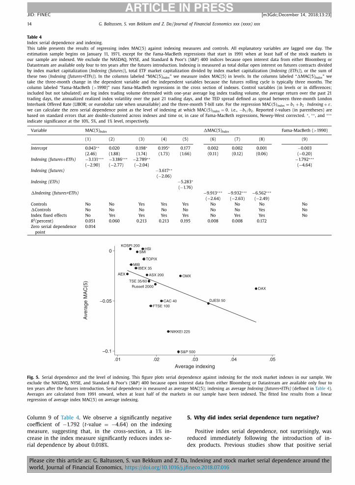
Table 4

Index serial dependence and indexing.

This table presents the results of regressing index MAC(5) against indexing measures and controls. All explanatory variables are lagged one day. The

estimation sample begins on January 11, 1971, except for the Fama-MacBeth regressions that start in 1991 when at least half of the stock markets in

our sample are indexed. We exclude the NASDAQ, NYSE, and Standard & Poor’s (S&P) 400 indices because open interest data from either Bloomberg or

Datastream are available only four to ten years after the futures introduction. Indexing is measured as total dollar open interest on futures contracts divided

by index market capitalization ( Indexing (futures) ), total ETF market capitalization divided by index market capitalization ( Indexing (ETFs) ), or the sum of

these two ( Indexing (futures+ETFs) ). In the columns labeled “MAC(5) index ” we measure index MAC(5) in levels. In the columns labeled “�MAC(5) index ” we

take the three-month change in the dependent variable and the independent variables because the futures rolling cycle is typically three months . The

column labeled “Fama-MacBeth ( > 1990)” runs Fama-MacBeth regressions in the cross section of indexes. Control variables (in levels or in differences;

included but not tabulated) are log index trading volume detrended with one-year average log index trading volume, the average return over the past 21

trading days, the annualized realized index volatility over the past 21 trading days, and the TED spread defined as spread between three-month London

Interbank Offered Rate (LIBOR; or eurodollar rate when unavailable) and the three-month T-bill rate. For the regression MAC (5) index = b 1 + b 2 · Indexing + ε,

we can calculate the zero serial dependence point as the level of indexing at which MAC (5) index = 0 , i.e., −b 1 /b 2 . Reported t -values (in parentheses) are

based on standard errors that are double-clustered across indexes and time or, in case of Fama-MacBeth regressions, Newey-West corrected. ∗ , ∗∗ , and ∗∗∗

indicate significance at the 10%, 5%, and 1% level, respectively.

Variable MAC(5) Index �MAC(5) Index Fama-MacBeth ( > 1990)

(1) (2) (3) (4) (5) (6) (7) (8) (9)

Intercept 0.043 ∗∗ 0.020 0.198 ∗ 0.195 ∗ 0.177 0.002 0.002 0.001 −0.003

(2.46) (1.88) (1.74) (1.73) (1.66) (0.11) (0.12) (0.06) ( −0.20)

Indexing (futures + ETFs) −3.131 ∗∗∗ −3.186 ∗∗∗ −2.789 ∗∗ −1.792 ∗∗∗

( −2.90) ( −2.77) ( −2.04) ( −4.64)

Indexing (futures) −3.617 ∗∗

( −2.06)

Indexing (ETFs) −5.283 ∗

( −1.76)

�Indexing (futures+ETFs) −9.913 ∗∗∗ −9.932 ∗∗∗ −6.562 ∗∗∗

( −2.64) ( −2.63) ( −2.49)

Controls No No Yes Yes Yes No No No No

�Controls No No No No No No No Yes No

Index fixed effects No Yes Yes Yes Yes No Yes Yes No

R 2 (percent) 0.051 0.060 0.213 0.213 0.195 0.008 0.008 0.172

Zero serial dependence

point

0.014

Fig. 5. Serial dependence and the level of indexing. This figure plots serial dependence against indexing for the stock market indexes in our sample. We

exclude the NASDAQ, NYSE, and Standard & Poor’s (S&P) 400 because open interest data from either Bloomberg or Datastream are available only four to

ten years after the futures introduction. Serial dependence is measured as average MAC(5); indexing as average Indexing (futures+ETFs) (defined in Table 4 ).

Averages are calculated from 1991 onward, when at least half of the markets in our sample have been indexed. The fitted line results from a linear

regression of average index MAC(5) on average indexing.

Column 9 of Table 4 . We observe a significantly negative

coefficient of −1.792 ( t -value = −4.64) on the indexing

measure, suggesting that, in the cross-section, a 1% in-

crease in the index measure significantly reduces index se-

rial dependence by about 0.018%.

Please cite this article as: G. Baltussen, S. van Bekkum and Z. Da

world, Journal of Financial Economics, https://doi.org/10.1016/j.jfi

5. Why did index serial dependence turn negative?

Positive index serial dependence, not surprisingly, was

reduced immediately following the introduction of in-

dex products. Previous studies show that positive serial

, Indexing and stock market serial dependence around the

neco.2018.07.016

G. Baltussen, S. van Bekkum and Z. Da / Journal of Financial Economics xxx (xxxx) xxx 15

ARTICLE IN PRESS

JID: FINEC [m3Gdc; December 14, 2018;13:23 ]

dependence results from market microstructure biases

such as price staleness and infrequent trading ( Fisher,

1966; Scholes and Williams, 1977; Atchison et al., 1987;

Lo and MacKinlay, 1990a; Boudoukh et al., 1994 , and ref-

erences cited therein) or lead-lag effects due to a response

to economy-wide information that is more sluggish for

some stocks than for others ( Brennan et al., 1993; Badri-

nath et al., 1995; Chordia and Swaminathan, 20 0 0; Mc-

Queen et al., 1996 ). 7

Equity index futures were the first instruments in many

countries that offered investors the opportunity to invest

in the index easily, cheaply, and continuously during trad-

ing hours. This could have improved the functioning of the

underlying stock markets in two ways. First, increased re-

sponsiveness to market-wide shocks and market makers

hedging their inventory position increase trading in the

smaller, less liquid index members, which attenuates mar-

ket microstructure biases such as price staleness. 8 Second,

trading in index futures speeds up the incorporation of

market-wide information for all stocks in the index so that

the lead-lag effect diminishes. These findings imply that

index serial dependence decreases to zero after the start of

indexing. Returns of index products themselves also should

have zero serial dependence because they are traded heav-

ily and continuously throughout the day and unlikely suf-

fer from information asymmetry ( Subrahmanyam, 1991;

Madhavan and Sobczyk, 2016 ).

In this paper, we find index serial dependence to not

just drop to zero but also turn significantly negative. In

addition, serial dependence in index product returns is

negative, from the moment these products are traded.

Negative index serial dependence suggests the existence

of non-fundamental shocks [e.g., price pressure as a com-

pensation for liquidity provision ( Campbell et al., 1993;

Nagel, 2012 )] even at the aggregate level. However, one

could argue that aggregate price pressure can come from

other factors such as increasing investor demand to trade

the market portfolio over time, which affects order flow

irrespective of the existence of index products. One could

even argue that the futures introduction date is completely

endogenous and that futures trading is introduced with

the purpose of catering to market-level order flow. To

address these concerns, in Section 5.1 , we perform a test

that directly links the decrease in serial dependence to

7 Other explanations are time-varying expected returns ( Conrad and

Kaul, 1988; Conrad et al., 1991 ), and contemporaneous correlations be-

tween, for example, large caps and small caps and own-portfolio autocor-

relations ( Hameed, 1997 ). However, follow-up studies suggest that these

explanations do not fully account for positive serial dependence. 8 So far, we have controlled for market microstructure biases to some

extent using the one-day “implementation” lag between the current re-

turns and the weighted sum of past returns in Eq. (2) (i.e., between the

formation and holding period). MAC(5) falls into negative territories with

and without the implementation lag in both index and the (large and very

liquid) futures and ETF markets. Also, MAC(5) is less susceptible to serial

dependence coming from stale prices than measures such as AR(1). Fur-

thermore, microstructure biases are unlikely to have a significant impact

on serial dependence for any well diversified index ( Lo and MacKinlay,

1990a ). Finally, when we decompose index-level serial dependence as in

Lo and MacKinlay (1990b) , both index constituents’ serial dependence and

their lead-lag effects turn negative. Hence, attenuated microstructure bi-

ases are unlikely to explain our key finding.

Please cite this article as: G. Baltussen, S. van Bekkum and Z. Da

world, Journal of Financial Economics, https://doi.org/10.1016/j.jfi

differential price pressures arising exogenously from the

index design. Following Greenwood (2008) , we examine

how indexing products change serial dependence for

small, overweighted Nikkei 225 members relative to large,

underweighted Nikkei 225 members.

One could also argue that index-level price pressure has

been constantly present over time but used to be over-

shadowed by stale prices, slow information diffusion, or

other factors causing positive serial dependence. Because

the introduction of index products eliminates these factors,

index serial dependence could have become discernibly

negative afterward without actually decreasing. To address

this concern, in Section 5.2 , we compare how indexing

products change serial dependence for an index based on

small S&P 500 stocks, relative to a control index of large

stocks that are at least as accurately priced and absorb in-

formation at least as quickly but are not a member of the

S&P 500.

Finally, in Section 5.3 , we investigate the important role

of index arbitrage in linking serial dependence in index

futures or ETFs to serial dependence in the index. In the

presence of index arbitrage, the popularity of index prod-

ucts opens up the underlying index to price pressure from

these products, and vice versa, thus contributing to the

spreading of serial dependence characteristics across mar-

kets.

5.1. The Nikkei 225 index versus the TOPIX

The value-weighted TOPIX and the price-weighted

Nikkei 225 index are two major equity indexes in Japan

that are equally important to investors but differ in their

constituent weighting scheme. While the TOPIX is value

weighted, the Nikkei 225 index is weighted using the share

price of Nikkei 225 member stocks and their par value at

the time of offering.

The par value of a common stock (i.e., the monetary

amount at which a share is issued or can be redeemed)

can be seen as a base for shares and is stated in the corpo-

rate charter. Shares cannot be sold below par at an initial

public offering (IPO), so that par values indicate the most

favorable issue price around an IPO. While this used to be

a valuable signal, par value lost its relevance to investors

once stock issuance prices were required to be published

publicly. Nowadays, in most countries, the par value of

stock serves only legal purposes.

In the Nikkei 225, par value for most stocks is 50 yen

per share but can also take values of 50 0, 5,0 0 0, or 50,0 0 0

yen per share. As a consequence, some of the smaller

(larger) stocks receive a relatively large (small) Nikkei

225 weight, which makes them overweighted (under-

weighted) in comparison with their market capitalization-

based weight in the TOPIX. Greenwood (2008) shows

that overweighted stocks receive proportionally more price

pressure and uses overweighting as an instrument for in-

dex demand. Thus, the Japanese market provides an attrac-

tive experimental setting to study the effect of indexing on

index serial dependence.

To calculate Nikkei 225 index weights, we collect the

history of TOPIX and Nikkei 225 index membership from

Compustat Global’s Index Constituents file. We obtain the

, Indexing and stock market serial dependence around the

neco.2018.07.016

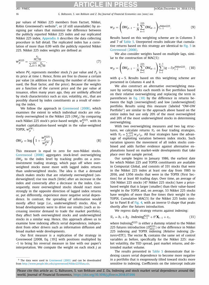
16 G. Baltussen, S. van Bekkum and Z. Da / Journal of Financial Economics xxx (xxxx) xxx

ARTICLE IN PRESS

JID: FINEC [m3Gdc; December 14, 2018;13:23 ]

par values of Nikkei 225 members from Factset, Nikkei,

Robin Greenwood’s website 9 , or (if still unavailable) by as-

signing par values that minimize the difference between

the publicly reported Nikkei 225 index and our replicated

Nikkei 225 index. Appendix A describes the data collecting

procedure in full detail. The replicated index has a corre-

lation of more than 0.99 with the publicly reported Nikkei

225. Nikkei 225 index weights are defined as

w

N225 jt =

P jt PV j / 50 ∑ 225

k =1 P kt

PV k / 50

, (7)

where PV j represents member stock j ’s par value and P jt is

its price at time t . Hence, firms are free to choose a certain

par value (in addition to choosing the number of shares is-

sued, the float factor, and the price). Because the weights

are a function of the current price and the par value at

issuance, often many years ago, they are unlikely affected

by stock characteristics such as size, volatility, etc., that are

possibly shared by index constituents as a result of enter-

ing the index.

We follow the approach in Greenwood (2008) , which

examines the extent to which individual stocks are rela-

tively overweighted in the Nikkei 225 ( OW jt ) by comparing

each Nikkei 225 stock’s price-based weight, w

N225 jt

, with its

market capitalization-based weight in the value-weighted

TOPIX, w

V W

jt :

OW jt = log

(1 +

w

N225 jt

w

V W

jt

). (8)

This measure is equal to zero for non-Nikkei stocks.

Greenwood (2008) aggregates stock-level overweighting

OW jt to the index level by tracking profits on a zero-

investment trading strategy, which pays off when over-

weighted stocks move more with lagged index returns

than underweighted stocks. The idea is that a demand

shock makes stocks that are relatively overweighted (un-

derweighted) rise too much (little) after an increase in the

index and conversely after a decrease in the index. Con-

sequently, more overweighted stocks should react more

strongly in the opposite direction of lagged index returns

or, put differently, experience more negative serial depen-

dence. In contrast, the spreading of information would

mostly affect lar ge (i.e., underweighted) stocks. Also, if

broad developments were to drive our results (such as in-

creasing investor demand to trade the market portfolio),

they affect both overweighted stocks and underweighted

stocks in a similar way. Hence, this approach allows us to

examine how indexing affects serial dependence, indepen-

dent from other drivers such as information diffusion and

broad market-wide developments.

Our first measure is a replication of the strategy in

Greenwood [2008, Eq. (19)] with positions multiplied by

-1 to bring his reversal measure in line with our paper’s

interpretation. We compute the weight on each stock j as

9 The data were used in Greenwood (2005) and can be downloaded

from http://www.people.hbs.edu/rgreenwood/Nikkei225Data.xls .

Please cite this article as: G. Baltussen, S. van Bekkum and Z. Da

world, Journal of Financial Economics, https://doi.org/10.1016/j.jfi

w jt =

(

OW jt−1 −1

N

225 ∑

n =1

OW nt−1

)

r Nikkei 225 t−1 . (9)

Results based on this weighting scheme are in Columns 3

and 7 of Table 5 . Unreported results indicate that cumula-

tive returns based on this strategy are identical to Fig. 5 in

Greenwood (2008) .

We also consider weights based on multiple lags, simi-

lar to the construction of MAC(5):

w jt =

(

OW jt−1 −1

N

225 ∑

n =1

OW nt−1

)

q −1 ∑

l=1

(q − l) r Nikkei 225 t−l , (10)

with q = 5 . Results based on this weighting scheme are

presented in Columns 4 and 8.

We also construct an alternative overweighting mea-

sure by sorting stocks each month in five portfolios based

on their relative overweighting and replacing the term in

parentheses in Eq. (10) by the difference in returns be-

tween the high (overweighted) and low (underweighted)

portfolio. Results using this measure (labeled “OW-UW

Portfolio”) are similar to the approach above based on the

entire index but use only 20% of the most overweighted

and 20% of the most underweighted stocks in determining

overweighting.

With two overweighting measures and two lag struc-

tures, we calculate returns R t on four trading strategies,

with R t ≡∑ 225

j=1 w jt r jt . All four strategies have the advan-

tage of exploiting variation between index stocks. Such

variation ignores the movement of all index stocks com-

bined and adds further evidence against alternative ex-

planations based on market-wide developments that take

place over the sample period.

Our sample begins in January 1986, the earliest date

for which Nikkei 225 and TOPIX constituents are available

in Compustat Global, and consists of 331 stocks that were

in the Nikkei 225 index at least one day from 1985 to

2016, and 1,956 stocks that were in the TOPIX (First Sec-

tion) for at least 60 trading days. Over time, an average of

156 Nikkei 225 stocks (47 Nikkei 225 stocks) have a price-

based weight that is larger (smaller) than their value-based

weight in the TOPIX and, on average, 53 Nikkei 225 stocks

have weights of more than five times their weight in the

TOPIX. Cumulative MAC(5) for the Nikkei 225 looks simi-

lar to Panel B of Fig. 4 , with an inverse U-shape that peaks

shortly after the futures introduction.

We regress daily strategy returns against indexing:

R t = b 1 + b 2 · Indexing N225 t−1 + θ ′ X t−1 + ε t , (11)

where Indexing N225 t is either a dummy related to the Nikkei

225 futures introduction ( D

N225 intro

) or the difference in Nikkei

225 indexing and TOPIX indexing ( Relative indexing (fu-

tures+ETF) ). The vector X t contains the same set of control

variables as before, specifically for the Nikkei 225: mar-

ket volatility, the TED spread, past market returns, and de-

trended market volume.

The results presented in Table 5 demonstrate that in-

dexing causes serial dependence to become more negative

in a portfolio that is exogenously tilted toward stocks more

sensitive to indexing. Coefficients on the intercept indicate

, Indexing and stock market serial dependence around the

neco.2018.07.016

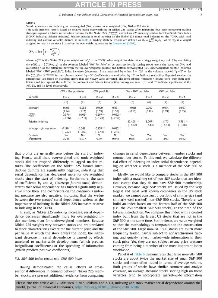
G. Baltussen, S. van Bekkum and Z. Da / Journal of Financial Economics xxx (xxxx) xxx 17

ARTICLE IN PRESS

JID: FINEC [m3Gdc; December 14, 2018;13:23 ]

Table 5

Serial dependence and indexing in overweighted (OW) versus underweighted (UW) Nikkei 225 stocks.

This table presents results based on relative index overweighting in Nikkei 225 stocks after regressing four zero-investment trading

strategies against a futures introduction dummy for the Nikkei 225 (“D N225 intro

”) and Nikkei 225 indexing relative to Tokyo Stock Price Index

(TOPIX) indexing ( Relative indexing ). Relative indexing is total indexing on the Nikkei 225 minus total indexing on the TOPIX, with total

indexing and control variables defined as in Table 4 . Trading strategy returns are defined as R t ≡∑ 225

j=1 w jt r jt , where w jt is a weight

assigned to return r on stock j based on the overweighting measure in Greenwood (2008) ,

OW jt = log

(1 +

w

N225 jt

w

VW jt

),

where w

N225 jt

is the Nikkei 225 price weight and w

VW jt

is the TOPIX value weight. We determine strategy weight w jt = A · B by calculating

A ≡(OW it−1 − 1

N

∑

OW jt−1

)in the columns labeled “OW Portfolio” or by cross-sectionally sorting stocks every day based on OW jt and

calculating A as the difference between the top overweighted quintile and bottom overweighted (i.e., underweighted) quintile (columns

labeled “OW - UW portfolio”). Index increases (decreases) B are measured by either B ≡ r N225 t−1 in the columns labeled “q = 2 ” or by

B ≡ ∑ 4 l=1 (5 − l) r Nikkei 225

t−l in the columns labeled “q = 5 .” Coefficients are multiplied by 10 4 to facilitate readability. Reported t -values (in

parentheses) are based on standard errors that are Newey-West corrected. The rows labeled “Intercept + futures intro ” sum both coef-

ficients and test against the null that the intercept and futures introduction dummy are zero. ∗ , ∗∗ , and ∗∗∗ indicate significance at the

10%, 5%, and 1% level, respectively.

OW - UW portfolio OW portfolio OW - UW portfolio OW portfolio

Variable q = 2 q = 5 q = 2 q = 5 q = 2 q = 5 q = 2 q = 5

(1) (2) (3) (4) (5) (6) (7) (8)

Intercept 0.195 0.055 0.099 0.031 −0.018 0.062 0.074 0.067

(1.24) (1.17) (1.59) (1.50) (-0.15) (0.72) (1.09) (1.65)

D N225 intro

−0.374 ∗∗ -0.102 ∗∗ −0.207 ∗∗∗ −0.052 ∗∗

( −2.36) ( −2.11) ( −3.20) ( −2.35)

Relative indexing −12.408 ∗∗∗ −3.767 ∗∗ −11.170 ∗∗∗ −3.591 ∗∗∗

( −4.12) ( −2.44) ( −4.93) ( −3.18)

Intercept + futures intro −0.180 ∗∗∗ −0.048 ∗∗∗ −0.108 ∗∗∗ −0.022 ∗∗

( −7.72) ( −3.60) ( −6.40) ( −2.45)

Controls No No No No Yes Yes Yes Yes

R 2 (percent) 0.235 0.077 0.174 0.048 0.851 0.549 1.063 0.562

that profits are generally zero before the start of index-

ing. Hence, until then, overweighted and underweighted

stocks did not respond differently to lagged market re-

turns. The coefficients on the Nikkei 225 futures intro-

duction dummy are significantly negative, indicating that

serial dependence has decreased more for overweighted

stocks since the start of indexing. Furthermore, the sum

of coefficients b 1 and b 2 ( Intercept+futures intro ) demon-

strates that serial dependence has turned significantly neg-

ative since then. The coefficients on the continuous index-

ing measure are also negative, indicating that the wedge

between the two groups’ serial dependence widens as the

importance of indexing in the Nikkei 225 increases relative

to indexing in the TOPIX.

In sum, as Nikkei 225 indexing increases, serial depen-

dence decreases significantly more for overweighted in-

dex members than for underweighted members. Because

Nikkei 225 weights vary between stocks and are unrelated

to stock characteristics except for the current price and the

par value at which the stock enters the index, the signif-

icant decrease in serial dependence is caused by effects

unrelated to market-wide developments (which predicts

insignificant coefficients) or the spreading of information

(which predicts positive coefficients).

5.2. S&P 500 index versus non–S&P 500 index

Having demonstrated the causal effects of cross-

sectional differences in demand between Nikkei 225 mem-

ber stocks, we present additional evidence from comparing

Please cite this article as: G. Baltussen, S. van Bekkum and Z. Da

world, Journal of Financial Economics, https://doi.org/10.1016/j.jfi

changes in serial dependence between member stocks and

nonmember stocks. To this end, we calculate the differen-

tial effect of indexing on index serial dependence, depend-

ing on whether a stock is a member of the S&P 500 or

not.

Ideally, we would like to compare stocks in the S&P 500

index with a matching set of non-S&P stocks that are iden-

tical except that they do not have S&P 500 membership.

However, because large S&P stocks are issued by the very

largest and most well known companies in the US stock

market, we cannot construct a portfolio of similar-size (and

similarly well tracked) non–S&P 500 stocks. Therefore, we

build an index based on the bottom half of the S&P 500

(i.e., the 250 smallest S&P 500 stocks) at the time of the

futures introduction. We compare this index with a control

index built from the largest US stocks that are not in the

S&P 500 at the same time. Both indexes are value weighted

so that the methodology is comparable to the construction

of the S&P 500. Large non–S&P 500 stocks are much more

frequently traded, hardly subject to nonsynchronous trad-

ing, and quickly reflect market-wide information in their

stock price. Yet, they are not subject to any price pressure

coming from being a member of the most important index

worldwide.

Panel A of Table 6 demonstrates that large non–S&P 500

stocks are about twice the market size of small S&P 500

stocks and more often traded in terms of average volume.

Both groups of stocks have similar turnover and analyst

coverage, on average. Because stocks scoring high on these

variables tend to incorporate market-wide information

, Indexing and stock market serial dependence around the

neco.2018.07.016

18 G. Baltussen, S. van Bekkum and Z. Da / Journal of Financial Economics xxx (xxxx) xxx

ARTICLE IN PRESS

JID: FINEC [m3Gdc; December 14, 2018;13:23 ]

Table 6

Serial dependence and indexing in Standard & Poor’s (S&P) 500 stocks versus large non-S&P 500 stocks.

This table compares subindex MAC(5) between a portfolio of the 250 stocks in the bottom half of the

S&P 500 and a portfolio of the 250 largest stocks that are not in the S&P 500. Panel A summarizes

market capitalization, volume, turnover, analyst coverage, and institutional ownership for the stocks

underlying each of the two subindexes. In Panel B, we regress subindex MAC(5) on an indicator vari-

able equal to one for observations based on the small S&P 500 member stocks and zero otherwise ( In

S&P ), indexing measures specifically for the S&P 500, control variables, and interactions between the In

S&P variable and each indexing measure. All explanatory variables are as defined in Table 4 and spe-

cific to the S&P 500. Reported t -values (in parentheses) are based on standard errors that are clustered

in the time dimension. ∗ , ∗∗ , and ∗∗∗ indicate significance at the 10%, 5%, and 1% level, respectively.

Panel A: Characteristics of member and non-member stocks

Variable Smallest 250 stocks in S&P Largest 250 stocks not in S&P

Average Standard deviation Average Standard deviation

(1) (2) (3) (4)

Market cap (billion of dollars) 2.561 3.384 5.194 11.100

Volume (billion) 0.825 3.227 1.228 7.794

Turnover 5.026 9.580 5.682 24.247

Analyst coverage 14.612 6.825 12.730 7.128

Inst. ownership 0.314 0.344 0.200 0.284

Panel B: Importance of S&P membership for decrease in serial dependence

Variable Subindex MAC(5)

(1) (2) (3) (4)

Intercept 0.174 ∗∗∗ 0.343 0.360 0.294

(9.39) (1.38) (1.39) (1.28)

In S&P 0.044 ∗∗∗

(2.71)

D S&P500 intro

−0.113 ∗∗∗

(-2.87)

In S&P ×D S&P500 intro

−0.156 ∗∗∗

( −3.66)

Indexing S&P500 −5.875 ∗

( −1.94)

In S&P × Indexing S&P500 −8.462 ∗∗∗

( −2.57)

Indexing S&P500 (futures) −9.586 ∗

( −1.79)

In S&P × Indexing S&P500 (futures) −14.24 ∗∗

( −2.46)

Indexing S&P500 (ETFs) −9.154 ∗∗

( −2.12)

In S&P × Indexing S&P500 (ETFs) −12.36 ∗∗∗

( −2.63)

Controls No Yes Yes Yes

Number of observations 23,200 23,200 23,200 23,200

R 2 (percent) 0.054 0.246 0.254 0.207

faster ( Lo and MacKinlay, 1990b; Chordia and Swami-

nathan, 20 0 0; Brennan et al., 1993 ), the large non-S&P

stocks can be expected to incorporate information at least

as fast as the small S&P 500 stocks, be easier to trade, and

be less subject to microstructure noise. Thus, serial depen-

dence should be similar or lower in the large non–S&P 500

subset if it were not for indexing. At the same time, the

small S&P 500 stocks have higher institutional ownership,

suggesting stronger institutional demand for index stocks.

In Panel B of Table 6 , we regress MAC(5) on an In S&P

dummy equal to one for the small S&P 500 index and zero

for the large non-S&P 500 index, interacted with one of

our measures for indexing,

MAC (5) it = b 1 + b 2 Indexing S& P500 t−1 + b 3 In S& P i + b 4 In S& P i

× Indexing S& P500 t−1 + θ ′ X t−1 + ε it , (12)

Please cite this article as: G. Baltussen, S. van Bekkum and Z. Da

world, Journal of Financial Economics, https://doi.org/10.1016/j.jfi

where MAC(5) captures the return on the two subindexes

i and Indexing S& P500 t is a dummy equal to one after the in-

troduction of indexing and zero otherwise ( D

S& P500 intro

, as in

Table 3 for the S&P 500) or one of the continuous indexing

variables from Table 4 [i.e., Indexing, Indexing (futures) and

Indexing (ETFs) for the S&P 500] . The vector X t contains the

same set of control variables as before, for the S&P 500:

market volatility, the TED spread, past market returns, and

detrended market volume. With only two subindexes, stan-

dard errors are clustered in the time dimension, but results

are similar or better with Newey-West or index-clustered

errors.

In Column 1 of Table 6 , Panel B, b 1 is significantly

positive, indicating that serial dependence is positive for

non–S&P 500 firms before the futures introduction. Coeffi-

cient b 3 is also significantly positive, indicating that, prior

, Indexing and stock market serial dependence around the

neco.2018.07.016

G. Baltussen, S. van Bekkum and Z. Da / Journal of Financial Economics xxx (xxxx) xxx 19

ARTICLE IN PRESS

JID: FINEC [m3Gdc; December 14, 2018;13:23 ]

to indexing, portfolio-level serial dependence is higher for

the small S&P 500 stocks than for the large non–S&P 500

stocks. This suggests that information diffuses faster across

the large, well-traded non–S&P 500 stocks up to the fu-

tures introduction. 10 The coefficient on the futures intro-

duction dummy ( b 2 ) indicates that serial dependence for

the large non–S&P 500 stocks decreases significantly af-

terward, from 0.174 to 0.061. However, the coefficient on

In S&P ×D

S&P500 intro

( b 4 ) shows that this decrease is signifi-

cantly more negative for the small S&P 500 members. In

fact, the sum of D

S&P500 intro

and In S&P ×D

S&P500 intro

coefficients

( b 2 + b 4 = −0 . 269 ) indicates that serial dependence steeply

decreases for these stocks into negative territory, from b 1 +b 3 = 0 . 218 (higher than for very large nonmember stocks)

to b 1 + b 2 + b 3 + b 4 = −0 . 051 (negative and lower than for

very large nonmember stocks). This result provides direct

evidence against a narrative that demand effects have al-

ways led to negative serial dependence in the past but be-

come discernible only once they are no longer offset by

factors that lead to positive serial dependence (such as

stale prices and slow information diffusion).

Results in Table 6 are similar when we add control vari-

ables and use the continuous indexing measures Indexing,

Indexing (futures) , and Indexing (ETFs) from Table 4 . Coeffi-

cients on the level of indexing are negative, indicative of

a downward trend in serial dependence as indexing in-

creases. Most importantly, the significantly negative inter-

action coefficients demonstrate that serial dependence de-

creases significantly more for the index based on small S&P

500 stocks. Thus, all columns in Table 6 point toward a sig-

nificant effect of index membership on serial dependence

that goes beyond explanations based on faster information

diffusion and reduced microstructure noise. 11

5.3. The index arbitrage mechanism

The fact that serial dependence is negative for both

the index and the index product is consistent with the

presence of arbitrage between the two. In this section, we

examine such index arbitrage in greater detail. Index arbi-

trage can propagate price pressure from the index product

to the underlying index, or vice versa. For instance,

Ben-David et al. (2018) argue that for continuously traded

index products such as ETFs, index arbitrage channels

serial dependence in index products into the underlying

index as liquidity providers hedge their exposure to the

index products by taking an offsetting position in the

10 This coefficient is significant at the 15% level with Newey-West stan-

dard errors. 11 To get some sense of the relative importance of these explanations,

we decompose the S&P 500 autocovariance terms from Eq. (2) into the

autocovariance of its constituents (i.e., reversals) and cross-autocovariance

across constituents (i.e., lead-lag effects) as in Lo and MacKinlay (1990b) .

We find that, prior to the futures introduction, both the lead-lag ef-

fect and the constituent-level reversal effect are significant. The futures

introduction has a negative effect on both components that is similar

in terms of their relative contributions to total autocovariance. This is

also true when we decompose S&P 500 autocovariance into the (cross-

)autocovariance of both constituents and sub-portfolios based on size, in-

dustry, volume, analyst coverage, or institutional ownership and when we

decompose the Nikkei 225 autocovariance into the (cross-)autocovariance

of constituents and size or industry sub-portfolios.

Please cite this article as: G. Baltussen, S. van Bekkum and Z. Da

world, Journal of Financial Economics, https://doi.org/10.1016/j.jfi

underlying index. This adds price pressure to the index

stocks in the same direction as for the index product.

After the price pressure disappears, the subsequent price

reversal generates negative serial dependence in both the

index and the index product.

Arbitrage per se says little about the underlying cause

of initial price pressure. Yet, as index futures and ETFs

become more popular and can be traded continuously

throughout the day, price pressure is likely to exist in in-

dex product markets and can spread through arbitrage.

Consequently, while stock markets used to be exposed to

price pressure only from individual stocks before the start

of indexing, now they are also exposed to price pressure

originating from index products such as futures and ETFs

through the arbitrage channel.

If index arbitrage spreads price pressures between the

index and the index product, we would expect index

MAC(5) to be closely related to index product MAC(5) [i.e.,

index MAC(5) = φ · index product MAC(5) with φ > 0]. Fur-

thermore, φ should be larger when more arbitrage activity

between the index products and the index takes place. To

examine the importance of arbitrage, we estimate φ and

see how it interacts with arbitrage activity. Arbitrage activ-

ity is likely to be higher in a market when index products

take a larger share of the market. Therefore, we use Index-

ing (Futures) or Indexing (ETFs) (measures from Section 5.2 )

to proxy for arbitrage activity.

We regress weekly index MAC(5) on weekly index prod-

uct MAC(5) to capture φ and its interaction with index-

ing:

MAC ( 5 ) index , it = b 1 + φ1 MAC ( 5 ) j, it + φ2 MAC ( 5 ) j, it

· Inde xin g j, it −5 + θ Inde xin g j, it −5 + ε it . (13)

with j = ET F or Futures . Indexing is measured at the start

of the weekly period over which we measure index MAC(5)

to avoid overlapping periods. To limit the impact of asyn-

chronous trading times between the futures and the index,

we compound daily (index product and index) MAC(5) re-

turns into weekly (Wednesday–Wednesday) returns. As be-

fore, different standard error adjustment methods lead to

similar standard error estimates. We include level versions

of all of the interacted variables and index fixed effects

(both unreported).

The stand-alone regression coefficients on futures

MAC(5) and ETF MAC(5), presented in Columns 1 and 3 of

Table 7 , are all positive and highly significant. Thus, index

MAC(5) significantly moves together with futures MAC(5)

and ETF MAC(5), suggesting the presence of index arbi-

trage. In Columns 2 and 4, we present results after inter-

acting this variable with Indexing . Coefficients on the in-

teraction terms are highly significant and positive for both

futures indexing and ETF indexing, indicating that more

arbitrage activity brings index MAC(5) significantly closer

to futures MAC(5). Therefore, as indexing products grow

in relative importance, index arbitrage becomes stronger

and negative serial dependence in the index becomes more

closely connected to serial dependence in the indexing

products.

, Indexing and stock market serial dependence around the

neco.2018.07.016

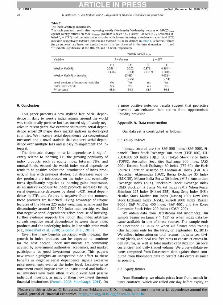
20 G. Baltussen, S. van Bekkum and Z. Da / Journal of Financial Economics xxx (xxxx) xxx

ARTICLE IN PRESS

JID: FINEC [m3Gdc; December 14, 2018;13:23 ]

Table 7

The index arbitrage mechanism.

This table presents results after regressing weekly (Wednesday-Wednesday) returns on MAC(5) index

against weekly returns on MAC(5) futures (columns labeled “ j = F utures ”) or MAC(5) ETF (columns la-

beled “ j = ET F ”), and the interaction variables with futures indexing or exchange traded fund (ETF)

indexing, respectively. Indexing (futures) and Indexing (ETFs) are defined in Table 4 . Reported t -values

(in parentheses) are based on standard errors that are clustered in the time dimension. ∗ , ∗∗ , and ∗∗∗ indicate significance at the 10%, 5%, and 1% level, respectively.

Weekly MAC(5) index

Variable j = F utures j = ET F

(1) (2) (3) (4)

Weekly MAC(5) j 0.558 ∗∗∗ 0.202 0.879 ∗∗∗ 0.861 ∗∗∗

(3.06) (0.83) (16.87) (11.04)

Weekly MAC(5) j × Indexing j 23.417 ∗∗∗ 8.052 ∗∗∗

(2.75) (2.53)

Level versions of interacted variables Yes Yes Yes Yes

Index fixed effects Yes Yes Yes Yes

R 2 (percent) 48.9 64.3 81.7 86.4

6. Conclusion

This paper presents a new stylized fact: Serial depen-

dence in daily to weekly index returns around the world

was traditionally positive but has turned significantly neg-

ative in recent years. We examine short-term serial depen-

dence across 20 major stock market indexes in developed

countries. We measure serial dependence via conventional

measures and a novel statistic that captures serial depen-

dence over multiple lags and is easy to implement and in-

terpret.

The dramatic change in serial dependence is signifi-

cantly related to indexing, i.e., the growing popularity of

index products such as equity index futures, ETFs, and

mutual funds. Around the world, index serial dependence

tends to be positive before the introduction of index prod-

ucts, in line with previous studies, but decreases once in-

dex products are introduced on the index and eventually

turns significantly negative as indexing gains importance.

As an index’s exposure to index products increases by 1%,

serial dependence decreases by about -0.031. Serial depen-

dence in ETFs and futures is negative from the moment

these products are launched. Taking advantage of unique

features of the Nikkei 225 index weighting scheme and the

discontinuity around S&P 500 index membership, we find

that negative serial dependence arises because of indexing.

Further evidence supports the notion that index arbitrage

spreads negative serial dependence between these index

products and the underlying index, in line with prior work

(e.g., Ben-David et al., 2018 ; Leippold et al., 2015 ).

Given the many benefits associated with indexing, the

growth in index products can be expected to continue

for the next decade. Index investments are commonly

advised by government authorities, academics, and market

participants as good investment practice. This paper’s

new result highlights an unexpected side effect to these

benefits as negative serial dependence signals excessive

price movements even at the index level. Excessive price

movement could impose costs on institutional and individ-

ual investors who trade often. It could even hurt passive

individual investors, as many of them now invest through

financial institutions ( French, 2008; Stambaugh, 2014 ). On

Please cite this article as: G. Baltussen, S. van Bekkum and Z. Da

world, Journal of Financial Economics, https://doi.org/10.1016/j.jfi

a more positive note, our results suggest that pro-active

investors can enhance their return from opportunistic

liquidity provision.

Appendix A. Data construction

Our data set is constructed as follows.

A.1. Equity indexes

Indexes covered are the S&P 500 index (S&P 500), Fi-

nancial Times Stock Exchange 100 index (FTSE 100), EU-

ROSTOXX 50 Index (DJESI 50), Tokyo Stock Price Index

(TOPIX), Australian Securities Exchange 200 Index (ASX

200), Toronto Stock Exchange 60 Index (TSE 60), the Paris

Bourse’s Cotation Assistée en Continu 40 Index (CAC 40),

Deutscher Aktienindex (DAX), Iberia Exchange 35 Index

(IBEX 35), Milano Italia Borsa 30 Index (MIB), Amsterdam

Exchange Index (AEX), Stockholm Stock Exchange Index

(OMX Stockholm), Swiss Market Index (SMI), Nihon Keizai

Shimbun 225 Index (Nikkei 225), Hang Seng Index (HSI),

Nasdaq Stock Market 100 Index (Nasdaq 100), New York

Stock Exchange Index (NYSE), Russell 20 0 0 Index (Russell

20 0 0), S&P MidCap 40 0 Index (S&P 400), and the Korea

Composite Stock Price 200 Index (KOSPI 200).

We obtain data from Datastream and Bloomberg. Our

sample begins on January 1, 1951 or when index data be-

came available in one of these sources. The sample ends

on December 31, 2016 or when all futures stop trading

(this happens only for the NYSE, on September 15, 2011).

We collect information on total returns, index prices, divi-

dend yields, and local risk free rates to construct excess in-

dex returns, as well as total market capitalization (in local

currencies) and daily traded volume. We cross-validate re-

turns computed from Datastream data against those com-

puted from Bloomberg data to correct data errors as much

as possible.

A.2. Equity futures

From Bloomberg, we obtain prices from front month fu-

tures contracts, which are rolled one day before expiry, to

, Indexing and stock market serial dependence around the

neco.2018.07.016

G. Baltussen, S. van Bekkum and Z. Da / Journal of Financial Economics xxx (xxxx) xxx 21

ARTICLE IN PRESS

JID: FINEC [m3Gdc; December 14, 2018;13:23 ]

construct futures returns. These contracts are the most liq-

uid futures, generally accounting for over 80% of the trad-

ing volume and open interest across all listed contracts on

an index. We collect information on futures prices from

Datastream to cross-check the Bloomberg futures data, and

to backfill Bloomberg’s futures returns when not covered

by Bloomberg. For the Nikkei 225, we focus on the futures

listed in the main market, Osaka. However, results are sim-

ilar when using contract prices from the Singapore Inter-

national Money Exchange (SIMEX) and Chicago Mercantile

Exchange (CME) listings. In addition, for the SMI, we use

futures data from Datastream prior to 1997, as Bloomberg

contains many stale quotes and misprints for this index be-

fore this date.

We also collect data on futures contract size (in listed

currencies per index point), volume, and open interest on

the futures and, in the case of the introduction of a mini-

futures or multiple listings on an index, we combine these

with data on the original listing. As several indexes have

multiple futures contracts written on them that vary in

terms of maturities and contract specifications (e.g., mini

versus regular futures), we obtain all futures series that

are written on our indexes. We aggregate these to reflect

total volume and open interest, in either local currencies

or number of contracts, with the number of contracts pro-

portional to the size of the contract that traded first (e.g.,

we assign a weight of 1/5 to the S&P 500 mini contract

because it trades for $100 per index point and the reg-

ular S&P 500 future has a size of $500 per index point).

Changes in contract size are retrieved from Datastream,

or publicly available online sources, or they are assumed

when prices increase or decrease with a factor two or

more.

A.3. Futures introductions

For futures introductions, we start with the earliest

date that futures data become available in Datastream

or Bloomberg. To determine whether we have the oldest

existing futures series, we cross-check this earliest date

with three sources: Ahn et al. (2002) , Gulen and Mayhew

(20 0 0) , and the website of the Commodity Research Bu-

reau (CRB), http://www.crbtrader.com/datacenter.asp .

A.4. ETFs

Several instances of a single ETF can be traded across

different countries or exchanges. To retrieve the set of

existing equity index ETFs, we obtain a list of all eq-

uity index ETFs on offer from a major broker-dealer

and cross-check with a list of all ETFs on offer by

another major broker-dealer. We include vanilla ETFs,

long and short index ETFs, levered ETFs or vanilla ETFs

on a levered index, ETFs with a currency hedge, and

all ETFs that are cross-listed. We collect information

from Bloomberg on ETF prices, market capitalization,

and volume. For each index, we add up the total

volume of contracts traded. We also calculate market

capitalization across all ETFs on a given index but subtract

inverse ETFs that offer short positions in the index and

multiply market capitalization for leveraged ETFs with the

Please cite this article as: G. Baltussen, S. van Bekkum and Z. Da

world, Journal of Financial Economics, https://doi.org/10.1016/j.jfi

leverage factor (typically one and a half, two, or three

times the index return). To prevent the impact of data

entry mistakes on our results, we set ETF observations to

missing for dates that report zero market cap or have a

market cap of less then 10% of the previous day’s market

cap. We then interpolate these observations from the last

trading day immediately before to the first day immedi-

ately after this date. We also experiment with removing

observations with open interest or an ETF market cap

more than five studentized residuals from its centered

one-year moving average, but this has a very limited

impact on the results.

A.5. S&P 500 constituents and other US stock data

For the S&P 500 constituents, we obtain the list of in-

dex constituents, as well as stock returns, shares outstand-

ing and turnover data, from CRSP, calculate analyst cov-

erage from Institutional Brokers’ Estimate System (I/B/E/S)

data, and retrieve data on institutional ownership from the

Thomson Financial 13f database. We replicate the S&P 500

index and the weights of each member using stock market

capitalizations. We use these data from July 1962 onward

as CRSP reports fewer than five hundred of the S&P’s index

members before this date. Further, we collect similar data

of all US stocks not included in the S&P 500 from the same

sources.

A.6. Nikkei 225 and TOPIX constituents

We collect the list of Nikkei 225 and TOPIX members

from Compustat Global, which begins in 1985. As some

constituents are merged or acquired and Compustat keeps

only the most recent company identifier, we use Factset to

cross-check the constituents in Compustat, identify stocks

with this problem, and collect identifying information on

such stocks before the takeover. Our sample of index con-

stituents represent 99.4% of TOPIX capitalization and in-

cludes all Nikkei 225 stocks. The remaining 0.6% comes

from very small stocks and we distribute them evenly

across all available stocks.

A.7. Nikkei 225 par values

As Nikkei does not provide information on par value

prior to 1998, we use the available information as starting

point. We obtain information on par values from a re-

cent constituent list on the exchange website ( https://

indexes.nikkei.co.jp/nkave/archives/file/nikkei _ stock _

average _ weight _ en.pdf ), a weightings list from Novem-

ber 1, 2011 available in Datastream, the raw data used

in Greenwood (2005) on Greenwood’s website, and the

weights on April 1, 1998, which is the earliest available

date for data provided by Nikkei. By combining Factset

with Compustat Global, we can determine the par values

of all index constituents from 20 0 0 onward (as this is

available in Factset), which we supplement with con-

stituents data for 1998 provided by Nikkei. For stocks that

are a member of the Nikkei 225 in 1986 or later but exit

the Nikkei 225 before 1998, we infer par values by mini-

mizing the difference between the Nikkei 225 index and

, Indexing and stock market serial dependence around the

neco.2018.07.016

22 G. Baltussen, S. van Bekkum and Z. Da / Journal of Financial Economics xxx (xxxx) xxx

ARTICLE IN PRESS

JID: FINEC [m3Gdc; December 14, 2018;13:23 ]

the aggregated price-weighted value of its constituents.

We set the par value to 50 (as most stocks have a par

value of 50) and change the par values to 50 0, 5,0 0 0, or

50,0 0 0 to minimize the daily tracking error between our

reconstructed index and the actual index.

A.8. Control variables

For market volatility, we use realized (annualized)

volatility over the last 21 days because it is available for

all indexes (as implied volatility indexes are not available

for many of them for a sufficiently long time). We use the

difference between the three-month US LIBOR (as of 1984)

or the eurodollar rate (between 1971 and 1984) and the

three-month US T-bill interest rate (obtained from the Fed-

eral Reserve Board St. Louis and Bloomberg) to calculate

the TED spread. We compute past market returns as the

past month (i.e., 21 trading days) market return as Hameed

et al. (2010) find that such a measure predicts serial de-

pendence profits. Finally, for market volume, we use the

log of index trading volume detrended by calculating the

five-day average relative to a one-year backward moving

average in the spirit of Campbell et al. (1993) .

Appendix B. Serial dependence as a variance difference

Autocovariance over a certain time period can be

replicated by the difference of two realized return vari-

ances that are evaluated over that same period T but

differ in the frequency over which they are calculated,

akin to variance difference statistics (see, for example,

Campbell et al. (1997) ). To see this, consider a short

(e.g., one week) period of length T , divided into q inter-

vals of equal length (e.g., five trading days), and a re-

turn from time 0 to T that equals the sum of the log

returns r t , t = 1 , . . . , T q with E(r t ) = μt = 0 . The variance

over the period T calculated over q intervals is Var (T , q ) =

Var (r 1 ) + Var (r 2 ) + · · · + Var (r q ) , or

Var (T , q ) =

q ∑

t=1

E(r 2 t ) =

q ∑

t=1

Var (r t ) . (14)

However, when we calculate the return over the same pe-

riod T , but over one instead of q intervals, the variance is

Var (T , 1) = E

⎡

⎣

(

q ∑

t=1

r t

) 2 ⎤

⎦

=

q ∑

t=1

Var (r t ) +

q −1 ∑

l=1

2(q − l) Cov (r t , r t−l ) . (15)

In Eq. (15) , Cov (r t , r t−l ) is the autocovariance in re-

turns between the current time unit t =

T q and its lag

t − l assuming that, over short intervals, Cov (r t , r t−l ) =

Cov (r k , r k −l ) ∀ t � = k (i.e., stationarity). Any serial correlation

causes Eq. (14) to deviate from Eq. (15) because the auto-

covariance terms are nonzero and the difference between

Eqs. (15) and (14) is simply a weighted sum of autocovari-

ance terms from lag 1 up to lag q − 1 .

The autocovariance term can be isolated as the differ-

ence in returns between two investment strategies over

Please cite this article as: G. Baltussen, S. van Bekkum and Z. Da

world, Journal of Financial Economics, https://doi.org/10.1016/j.jfi

period T (i.e., one that rebalances every interval q and one

that buys and holds over the period T ). First, after each of

the q intervals, a rebalancing strategy adjusts its position

to the initial position. As the price of the asset P changes

over time, profits after interval t amount to P t /P t−1 − 1 =

exp (r t ) − 1 and accumulate over period T to

q ∑

t=1

( exp (r t ) − 1 ) . (16)

Approximating exp ( r t ) with a second-order Taylor expan-

sion around zero, exp (x ) ≈ 1 + x +

1 2 x

2 , we can rewrite the

realized profits on the rebalancing strategy as

q ∑

t=1

(r t +

1

2

r 2 t

)=

q ∑

t=1

r t +

1

2

Var (T , q ) , (17)

where, over short periods, ∑ q

t=1 r 2 t ≈ Var (T , q ) .

By similar arguments, the realized profit on a second,

buy-and-hold strategy is

exp

(

q ∑

t=1

r t

)

− 1 =

q ∑

t=1

r t +

1

2

(

q ∑

t=1

r t

) 2

=

q ∑

t=1

r t +

1

2

Var (T , 1) (18)

The difference between the buy-and-hold strategy and the

rebalancing strategy then equals

1

2

Var (T , 1) − 1

2

Var (T , q ) =

q −1 ∑

l=1

(q − l) Cov (r t , r t−l ) . (19)

Thus, the variance difference in Eq. (1) , an often used

statistic to measure serial dependence, is equivalent to a

simple trading strategy that replicates the return autoco-

variances above by taking q − 1 positions as r t ∑ q −1

l= l (q −l) r t−l , l = 1 , . . . , q − 1 . For instance, to measure the serial

dependence in one week of daily returns, q = 5 (a common

horizon), one can take a position 4 r t−1 + 3 r t−2 + 2 r t−3 +1 r t−4 . Then, the daily return on our strategy is simply

r t (4 r t−1 + 3 r t−2 + 2 r t−3 + 1 r t−4 ) , which we scale into auto-

correlations as

MAC (5) = r t (4 r t−1 + 3 r t−2 + 2 r t−3 + 1 r t−4 ) / (5 · σ 2 ) . (20)

MAC(5) is equivalent to the (scaled) dollar difference be-

tween the buy-and-hold strategy and the rebalancing strat-

egy, as ∑ q −1

l=1 (q − l) E

[r t , r t−k

]=

∑ q −1

l=1 (q − l) Cov (r t , r t−k ) .

References

Ahn, D.-H. , Boudoukh, J. , Richardson, M. , Whitelaw, R.F. , 2002. Partial ad-

justment or stale prices? Implications from stock index and futures return autocorrelations. Rev. Financ. Stud. 15 (2), 655–689 .

Atchison, M.D. , Butler, K.C. , Simonds, R.R. , 1987. Nonsynchronous security trading and market index autocorrelation. J. Finance 42 (1), 111–118 .

Avramov, D. , Chordia, T. , Goyal, A. , 2006. Liquidity and autocorrelations in

individual stock returns. J. Finance 61 (5), 2365–2394 . Badrinath, S.G. , Kale, J.R. , Noe, T.H. , 1995. Of shepherds, sheep, and

the cross-autocorrelations in equity returns. Rev. Financ. Stud. 8 (2), 401–430 .

Barberis, N. , Shleifer, A. , Wurgler, J. , 2005. Comovement. J. Financ. Econ.75 (2), 283–317 .

, Indexing and stock market serial dependence around the

neco.2018.07.016

G. Baltussen, S. van Bekkum and Z. Da / Journal of Financial Economics xxx (xxxx) xxx 23

ARTICLE IN PRESS

JID: FINEC [m3Gdc; December 14, 2018;13:23 ]

Ben-David, I., Franzoni, F., Moussawi, R., 2018. Do ETFs increase volatility?J. Finance . https://doi.org/10.1111/jofi.12727 . Forthcoming.

Bhattacharya, A. , O’Hara, M. , 2015. Can ETFs increase market fragility? Ef-fect of information linkages in ETF markets . Unpublished working pa-

per, Cornell University, Ithaca, NY. Bogle, J.C. , 2014. Lightning strikes: the creation of Vanguard, the first in-

dex mutual fund, and the revolution it spawned. J. Portf. Manag. 40

(5), 42–59 . Bond, P. , García, D. , 2017. The equilibrium consequences of indexing . Un-

published working paper, University of Washington and University ofColorado Boulder, Seattle, WA, and Boulder, CO.

Boudoukh, J. , Richardson, M.P. , Whitelaw, R. , 1994. A tale of three schools:insights on autocorrelations of short-horizon stock returns. Rev. Fi-

nanc. Stud. 7 (3), 539–573 . Brennan, M.J. , Jegadeesh, N. , Swaminathan, B. , 1993. Investment analysis

and the adjustment of stock prices to common information. Rev. Fi-

nanc. Stud. 6 (4), 799–824 . Campbell, J.Y. , Grossman, S.J. , Wang, J. , 1993. Trading volume and serial

correlation in stock returns. Q. J. Econ. 108 (4), 905–939 . Campbell, J.Y. , Lo, A.W. , MacKinlay, A.C. , 1997. The Econometrics of Finan-

cial Markets. Princeton University Press, Princeton, NJ . Chan, K. , 1990. Information in the cash market and stock index futures

market. Ohio State University, Columbus, OH PhD dissertation .

Chan, K. , 1992. A further analysis of the lead-lag relationship between thecash market and stock index futures market. Rev. Financ. Stud. 5 (1),

123–152 . Chen, H. , Noronha, G. , Singal, V. , 2004. The price response to S&P 500

index additions and deletions: evidence of asymmetry and a new ex-planation. J. Finance 59 (4), 1901–1930 .

Chordia, T. , Roll, R. , Subrahmanyam, A. , 2005. Evidence on the speed of

convergence to market efficiency. J. Financ. Econ. 76 (2), 271–292 . Chordia, T. , Roll, R. , Subrahmanyam, A. , 2008. Liquidity and market effi-

ciency. J. Financ. Econ. 87 (2), 24 9–26 8 . Chordia, T. , Swaminathan, B. , 20 0 0. Trading volume and cross-autocorre-

lations in stock returns. J. Finance 55 (2), 913–935 . Conrad, J. , Kaul, G. , 1988. Time-variation in expected returns. J. Bus. 61

(4), 409–425 .

Conrad, J. , Kaul, G. , 1989. Mean reversion in short-horizon expected re-turns. Rev. Financ. Stud. 2 (2), 225–240 .

Conrad, J. , Kaul, G. , 1998. An anatomy of trading strategies. Rev. Financ.Stud. 11 (3), 489–519 .

Conrad, J. , Kaul, G. , Nimalendran, M. , 1991. Components of short-horizonindividual security returns. J. Financ. Econ. 29 (2), 365–384 .

Da, Z. , Shive, S. , 2017. Exchange traded funds and asset return correlations.

Eur. Financ. Manag. 24 (1), 136–168 . Duffie, D. , 2010. Presidential address: asset price dynamics with slow–

moving capital. J. Finance 65 (4), 1237–1267 . Etula, E. , Rinne, K. , Suominen, M. , Vaittinen, L. , 2015. Dash for cash: mon-

th-end liquidity needs and the predictability of stock returns . Un-published working paper, New York University and Aalto University

School of Business, New York, NY and Greater Helsinki, Finland.

Fama, E.F. , 1965. The behavior of stock market prices. J. Bus. 38 (1),34–105 .

Fama, E.F. , French, K.R. , 1988. Permanent and temporary components ofstock prices. J. Polit. Econ. 96 (2), 246–273 .

Fisher, L. , 1966. Some new stock market indexes. J. Bus. 39 (1), 191–225 . French, K.R. , 2008. Presidential address: the cost of active investing. J. Fi-

nance 63 (4), 1537–1573 . Greenwood, R. , 2005. Short- and long-term demand curves for stocks:

theory and evidence on the dynamics of arbitrage. J. Financ. Econ. 75

(3), 607–649 .

Please cite this article as: G. Baltussen, S. van Bekkum and Z. Da

world, Journal of Financial Economics, https://doi.org/10.1016/j.jfi

Greenwood, R. , 2008. Excess comovement of stock returns: evidence fromcross-sectional variation in Nikkei 225 weights. Rev. Financ. Stud. 21

(3), 1153–1186 . Gulen, H. , Mayhew, S. , 20 0 0. Stock index futures trading and volatility in

international equity markets. J. Futures Mark. 20 (7), 661–685 . Hameed, A. , 1997. Time-varying factors and cross-autocorrelations in

short-horizon stock returns. J. Financ. Res. 20 (4), 435–458 .

Hameed, A. , Kang, W. , Viswanathan, S. , 2010. Stock market declines andliquidity. J. Finance 65 (1), 257–293 .

Hawawini, G.A. , 1980. Intertemporal cross-dependence in securities dailyreturns and the short-run intervaling effect on systematic risk. J. Fi-

nanc. Quant. Anal. 15 (01), 139–149 . Hong, H. , Kubik, J.D. , Fishman, T. , 2012. Do arbitrageurs amplify economic

shocks? J. Financ. Econ. 103 (3), 454–470 . Hou, K. , 2007. Industry information diffusion and the lead-lag effect in

stock returns. Rev. Financ. Stud. 20 (4), 1113–1138 .

Israeli, D. , Lee, C.M. , Sridharan, S. , 2014. Is there a dark side to exchange–traded funds (ETFs)? An information perspective . Unpublished work-

ing paper, Stanford University, Stanford, CA. Jegadeesh, N. , 1990. Evidence of predictable behavior of security returns.

J. Finance 45 (3), 881–898 . Jylhä, P. , Rinne, K. , Suominen, M. , 2014. Do hedge funds supply or demand

liquidity? Rev. Finance 18 (4), 1259–1298 .

Lehmann, B.N. , 1990. Fads, martingales, and market efficiency. Q. J. Econ.105 (1), 1–28 .

Leippold, M. , Su, L. , Ziegler, A. , 2015. Do index futures and ETFs affectstock return correlations? . Unpublished working paper, University of

Zurich, Zurich, Switzerland. Lo, A.W. , MacKinlay, A.C. , 1988. Stock market prices do not follow random

walks: evidence from a simple specification test. Rev. Financ. Stud. 1

(1), 41–66 . Lo, A.W. , MacKinlay, A.C. , 1990a. An econometric analysis of nonsyn-

chronous trading. J. Econom. 45 (1), 181–211 . Lo, A.W. , MacKinlay, A.C. , 1990b. When are contrarian profits due to stock

market overreaction? Rev. Financ. Stud. 3 (2), 175–205 . Madhavan, A. , Sobczyk, A. , 2016. Price dynamics and liquidity of ex-

change-traded funds. J. Invest. Manag. 14 (2), 1–17 .

McQueen, G. , Pinegar, M. , Thorley, S. , 1996. Delayed reaction to good newsand the cross-autocorrelation of portfolio returns. J. Finance 51 (3),

889–919 . Nagel, S. , 2012. Evaporating liquidity. Rev. Financ. Stud. 25 (7), 2005–2039 .

O’Hara, M. , Ye, M. , 2011. Is market fragmentation harming market quality?J. Financ. Econ. 100 (3), 459–474 .

Richardson, M. , Smith, T. , 1994. A unified approach to testing for serial

correlation in stock returns. J. Bus. 67 (3), 371–399 . Scholes, M. , Williams, J. , 1977. Estimating betas from nonsynchronous

data. J. Financ. Econ. 5 (3), 309–327 . Schwartz, R.A. , Whitcomb, D.K. , 1977. The time-variance relationship: evi-

dence on autocorrelation in common stock returns. J. Finance 32 (1),41–55 .

Stambaugh, R.F. , 2014. Presidential address: investment noise and trends.

J. Finance 69 (4), 1415–1453 . Subrahmanyam, A. , 1991. A theory of trading in stock index futures. Rev.

Financ. Stud. 4 (1), 17–51 . Tosini, P.A. , 1988. Stock index futures and stock market activity in October

1987. Financ. Anal. J. 44 (1), 28–37 . Wurgler, J. , 2011. On the economic consequences of index-linked invest-

ing. In: Allen, W.T., Khurana, R., Rosenfeld, G. (Eds.), Challenges toBusiness in the Twenty-First Century: The Way Forward. American

Academy of Arts and Sciences, Cambridge, MA .

, Indexing and stock market serial dependence around the

neco.2018.07.016