Journal of Banking Finance - Columbia Universityvhd1/banking.pdf · Journal of Banking & Finance...
15
Journal of Banking & Finance xxx (2010) xxx-xxx Contents lists available at ScienceDirect Journal of Banking & Finance journal homepage: www.elsevier.com/locatelibf International diversification: A copula approach Loran Chollete a,*, Victor de la Pena b, Ching-Chih Lu c 'University of Stavanger, Stavanger N·4036, Norway b Columbia University, New York, NY 10027, USA C National Chengchi University, 64 Sec. 2, 2M-Nan Road, Taipei 116, Taiwan ARTICLE INFO ABSTRACT Article history: The viability of international diversification involves balancing benefits and costs. This balance hinges on Received 29 June 2009 the degree of asset dependence. In light of theoretical research linking diversification and dependence. Accepted 18 August 2010 we examine international diversification using two measures of dependence: correlations and copulas. Available online xxxx We document several findings. First. dependence has increased over time. Second, we find evidence of asymmetric dependence or downside risk in latin America. but less in the GS. The results indicate very JEL classification: little downside risk in East Asia. Third, East Asian and latin American returns exhibit some correlation (14 complexity, Interestingly. the regions with maximal dependence or worst diversification do not com- F30 G1S mand large returns. Our results suggest international limits to diversification, Tbey are also consistent with a possible tradeoff between intemational diversification and systemic risk. Keywords: Diversification Copula Correlation complexity Downside risk Systemic risk 1. Introduction The net benefit of international diversification is of great impor- tance in today's economic climate. In general. tbe tradeoff between diversification's benefits and costs binges on the degree of depen- dence across securities. as observed by Samuelson (1967). Ibragi- mov et al, (2009b). Shin (2009). Veldkamp and Van Nieuwerburgh (2010), and Bai and Green (2010). among others, Economists and investors often assess diversification benefits using a measure of dependence, such as correlation.! It is therefore vital to have accu- rate measures of dependence, There are several measures available in finance, including the traditional correlation and copulas. While each approach has advantages and disadvantages, researchers have rarely compared them in the same empirical study.2 Such reliance * Corresponding author. TeL: +47 51831500: fax: +47 51831550, E-mail addresses:[email protected] (L. Chollete), [email protected] (V. de la Penal. [email protected],tw (C-C Lu), 1 See Solnik (1974). Ingersoll (1987, Chapter 4); Carrieri et at. (2008): You and Daigler (2010), Moreover, asset prices. which reflect their diversification benefits in equilibrium. are assessed using dependence or covariance. See research on (APM and stochastic discount methods, such as Sharpe (1964). Lintner (1965), Lucas (1978). and Hansen and Singleton (1982), 2 Throughout, we use the word dependence as an umbrella to cover any situation where two or more variables move together. We adopt this practice because there are numerous words in use (e,g, correlation, concordant'e, co-dependency, comovement), and we wish to use a general term. We do not assume that any dependence measure is ideal. and throughout we indicate advantages and disadvantages as the case may be. 'D 2010 Elsevier B.V, All rights reserved, on one dependence measure prevents easy assessment of the degree of international diversification opportunities. and how they differ over time or across regions. The main goal of this paper is to assess diversification opportuni- ties available in international stock markets. using both correlations and copulas. The recent history of international markets is interest- ing in itself. due to the large number of financial crises, increasingly globalized markets, and financial contagion. 3 We also examine some basic implications for international asset pricing. In particular, we investigate whether the diversification measures are related to inter- national stock returns. This research is valuable because consider- ations of diversification and dependence should affect risk premia. A secondary focus of our paper is the relation between diversi- fication and systemic risk. We motivate this aspect by theoretical research such as Brumelle (1974), Ibragimov et al. (2009b). and Shin (2009), and it concerns two separate. distributional proper- ties: heavy tails and tail dependence. The term 'heavy tail' refers to the tail mass of the marginal, univariate distributions. while 'tail dependence' refers to the connection between marginal distribu- tions at extreme quantiles. 4 While no general theoretical results link , See Dungey and Tambakis (2005), Reinhart (2008), Reinhart and Rogoff (2009), Markwat et al, (2009), and Dungey et al, (2010). 4 We formally define tail dependence and tail indices in Eqs. (5) and (9), Further, we estimate both heavy tails and dependence in Tables 8 and 9, and Table II. respectively, 0378-4266/$ - see front matter © 2010 Elsevier B.V. All rights reserved, doi: I0, 1016/j.jbankfin.201 0.08.020
Transcript of Journal of Banking Finance - Columbia Universityvhd1/banking.pdf · Journal of Banking & Finance...

Journal of Banking amp Finance xxx (2010) xxx-xxx
Contents lists available at ScienceDirect
Journal of Banking amp Finance
journal homepage wwwelseviercomlocatelibf
International diversification A copula approach
Loran Chollete a Victor de la Pena b Ching-Chih Lu c
University of Stavanger Stavanger Nmiddot4036 Norway b Columbia University New York NY 10027 USA C National Chengchi University 64 Sec 2 2M-Nan Road Taipei 116 Taiwan
ARTICLE INFO ABSTRACT
Article history The viability of international diversification involves balancing benefits and costs This balance hinges on Received 29 June 2009 the degree of asset dependence In light of theoretical research linking diversification and dependence Accepted 18 August 2010 we examine international diversification using two measures of dependence correlations and copulas Available online xxxx We document several findings First dependence has increased over time Second we find evidence of
asymmetric dependence or downside risk in latin America but less in the GS The results indicate very JEL classification little downside risk in East Asia Third East Asian and latin American returns exhibit some correlation (14
complexity Interestingly the regions with maximal dependence or worst diversification do not comshyF30 G1S mand large returns Our results suggest international limits to diversification Tbey are also consistent
with a possible tradeoff between intemational diversification and systemic risk Keywords Diversification Copula Correlation complexity Downside risk Systemic risk
1 Introduction
The net benefit of international diversification is of great imporshytance in todays economic climate In general tbe tradeoff between diversifications benefits and costs binges on the degree of depenshydence across securities as observed by Samuelson (1967) Ibragishymov et al (2009b) Shin (2009) Veldkamp and Van Nieuwerburgh (2010) and Bai and Green (2010) among others Economists and investors often assess diversification benefits using a measure of dependence such as correlation It is therefore vital to have accushyrate measures of dependence There are several measures available in finance including the traditional correlation and copulas While each approach has advantages and disadvantages researchers have rarely compared them in the same empirical study2 Such reliance
Corresponding author TeL +47 51831500 fax +47 51831550
E-mail addressesiorangcholleteuisno (L Chollete) vpstatcolumbiaedll (V de la Penal cclunccuedutw (C-C Lu)
1 See Solnik (1974) Ingersoll (1987 Chapter 4) Carrieri et at (2008) You and Daigler (2010) Moreover asset prices which reflect their diversification benefits in equilibrium are assessed using dependence or covariance See research on (APM and stochastic discount methods such as Sharpe (1964) Lintner (1965) Lucas (1978) and Hansen and Singleton (1982)
2 Throughout we use the word dependence as an umbrella to cover any situation where two or more variables move together We adopt this practice because there are numerous words in use (eg correlation concordante co-dependency comovement) and we wish to use ageneral term We do not assume that any dependence measure is ideal and throughout we indicate advantages and disadvantages as the case may be
D 2010 Elsevier BV All rights reserved
on one dependence measure prevents easy assessment of the degree of international diversification opportunities and how they differ over time or across regions
The main goal of this paper is to assess diversification opportunishyties available in international stock markets using both correlations and copulas The recent history of international markets is interestshying in itself due to the large number of financial crises increasingly globalized markets and financial contagion3 We also examine some basic implications for international asset pricing In particular we investigate whether the diversification measures are related to intershynational stock returns This research is valuable because considershyations of diversification and dependence should affect risk premia
A secondary focus of our paper is the relation between diversi shyfication and systemic risk We motivate this aspect by theoretical research such as Brumelle (1974) Ibragimov et al (2009b) and Shin (2009) and it concerns two separate distributional propershyties heavy tails and tail dependence The term heavy tail refers to the tail mass of the marginal univariate distributions while tail dependence refers to the connection between marginal distribushytions at extreme quantiles4 While no general theoretical results link
See Dungey and Tambakis (2005) Reinhart (2008) Reinhart and Rogoff (2009) Markwat et al (2009) and Dungey et al (2010)
4 We formally define tail dependence and tail indices in Eqs (5) and (9) Further we estimate both heavy tails and dependence in Tables 8 and 9 and Table II respectively
0378-4266$ - see front matter copy 2010 Elsevier BV All rights reserved doi I0 1016jjbankfin201 008020
2 L (holere et atJournal of Banking amp finance xxx (201O) xxx-xxx
tail dependence and diversification dependence at extremes is conshysidered important from a risk management policy and broad ecoshynomic perspective This is particularly true in light of the ongoing financial recessions Consequently tail dependence forms the basis for many measures of systemic risks Regarding heavy tails researchers have established results that relate heavy tails diversifishycation and systemic risk These results show that when portfolio disshytributions are heavy-tailed not only do they represent limited diversification they may also suggest existence of a wedge between individual risk and systemic risk Thus there are aggregate ecoshynomic ramifications for heavy-tailed assets Specifically in a heashyvy-tailed portfolio environment diversification may yield both individual benefits and aggregate systemic costs If systemic costs are too severe the economy may require a coordinating agency to improve resource allocations Such policy considerations are absent from previous empirical research on heavy tails in international markets and provide a further motivation for our paper
The remaining structure of the paper is as follows In Section 2 we review theoretical and empirical literature on diversification and dependence In Section 3 we compare and contrast diversificashytion measures used in empirical finance Section 4 discusses our data and main results Section 5 illustrates some financial implicashytions and Section 6 concludes
2 Diversification dependence and systemic risk
The notion that diversification improves portfolio performance pervades economics and appears in asset pricing insurance and international finance A central precept is that based on the law of large numbers the return variance on a portfolio of a group of securities is lower than that of any single security9 An important caveat noted as early as Samuelson (1967) concerns the depenshydence structure of security returns as we discuss below This theoshyretical importance of dependence structure motivates our use of copulas in the empirical analysis
Diversification depends on both the dependence and marginal properties Since our initial focus is on dependence we will discuss its implications for diversification Jor a given set ofmarginals unless otherwise noted 10 Therefore when we describe a set of assets with lower dependence as having higher diversification benefits it is alshyways with the caveat that we are considering the marginals to be fixed
21 Theoretical background
When portfolios are heavy-tailed diversification may not be optimaL I I In an early important paper Samuelson (1967) examines
5 Economic examples of dependence at extreme periods may include the liquidity trap of Keynes (1936) and the nonlinear Phillips curve of Phelps (1968)
6 For measures of systemic risk derived from tail dependence see Hartmann et aJ (2003) Cherubini et aJ (2004 p 43) and Adrian and Brunnermeier (2008) For a discussion related to tail dependence and portfolio riskiness see Kortschak and Albrecher (2009)
7 For evidence on limited diverSification see Embrechts et aJ (2002) and Ibragimov and Walden (2007) For evidence on a wedge between individual risk and systemic risk see Ibragimov et at (2009~) and lbragimov et at (2009b)
8 For related work see Ibragimov et at (2009a) Chollete (2008) and Shin (2009) 9 The following authors formalize aspects of this precept Markowitz (1952)
Sharpe (1964) lintner (1965) Mossin (1966) and Samuelson (1967) 10 In this paper we transform all marginals to uniform by first ranking the data
Evidently if we were performing a dynamic study the marginals would vary and we would have a further reason to consider both marginals and dependence when discussing diversification
11 See Embrechts el at (2005) and Ibragimov (2009)
the restrictive conditions needed to ensure that diversification is optimal 12 He underscores the need for a general definition of negshyative dependence framed in terms of the distribution function of security returns In a significant development Brumelle (1974) proves that negative correlation is neither necessary nor sufficient for diversification except in special cases such as normal distribushytions or quadratic preferences Brumelle uses a form of dependence as a sufficient condition for diversification that involves the shape of the entire distribution Thus shortly after the inception of modshyern portfolio theory both Brumelle (1974) and Samuelson (1967) realize and discuss the need for restrictions on the joint distribushytion in order to obtain diversification However that discussion has a gap it stops short of examining multivariate (n gt 2) asset reshyturns and the practical difficulty of imposing dependence restricshytions on empirical data The use of copulas may be one way to fill this gap13 The research of Embrechts et al (2002) introduces copshyulas into risk management The authors first show that standard Pearson correlations can go dangerously wrong as a risk measure They then suggest the copula function as a flexible alternative to correlation which can capture dependence throughout the entire distribution of asset returns A copula C is by definition a joint disshytribution with uniform marginals In the bivariate case that means
C(u v) Pr[U u V ~ vJ (1 )
where U and Vare uniformly distributed on [01 J14 The intuition behind copulas is that they couple or join marshy
ginals into a joint distribution Copulas often have convenient parametric forms and summarize the dependence structure beshytween variables1s Specifically for any joint distribution Fxrlx y) with marginals Fxx) and FriY) we can write the distribution as
Fxr(xY) C(Fx(x) Fy(y)) (2)
for some copula C The usefulness of(2) is that we can simplify analshyysis of dependence in a return distribution Fxrlx y) by studying inshystead a copula C Since copulas represent dependence of arbitrary distributions in principle they allow us to examine diversification effects for heavy-tailed joint distributions following the logic of Brumelle (1974) and Samuelson (1967)
The above approaches analyze investor decisions and say litshytle about systemic risk Evidently investors decisions in aggreshygate may have an externality effect on financial and economic markets The existence of externalities related to excessive diversification has been emphasized by several recent papers We discuss the following three articles since their results focus on distributional properties16 lbragimov et aJ (2009b) develop a
Samuelson (1967) discusses several approaches to obtain equal investment in all assets as well as positive diversification in at least one asset The distributional assumptions on security returns involve ijd and strict independence of at least one security Although both utility functions and distributional assumptions are relevant Samuelson focuses on distributional concerns A special case of dependence when diversification may be optimal is that of perfeer negative correlation However if a portfolio consists of more than two assets some of which are negatively correlated then at least two must be positively correlated This could still result in suboptimality of diversification for at leaSI one asset when there are short sale constraints See Ibragimov (2009) and Samuelson (1967 p 7) 13 Another approach involves extreme value theory which we explore elsewhere See de la Pena et al (2006 Definition 31) It is typical to express the copula in
terms of the marginal distributions Fx(x) and Fy) In general the transformations from X and Y to their distributions fx and Fy are known as probability integral transforms and Fx and Fy can be shown to be uniformly distributed See Cherubini er al (2004 p 52) and Embrechts (2009)
15 This result holds for multivariate (n gt 2) quantities It is due to Sklar (l959) who proves that copulas uniquely characterize continuous distributions For non-continshyuous distributions the copula will not necessarily be unique In such situations the empirical copula approach of Deheuvels (1979) helps narrow down admissible copulas
16 Other papers include Krishnamurthy (2009) Shin (2009) Danielsson el al (2009) and Beine et al (2010)
3 L (holete et alfJoumal ofBanking amp Finance xxx (2010) xxx-xxx
model of catastrophic risks They characterize the existence of nonshydiversification traps situations where insurance providers may not insure catastrophic risks nor participate in reinsurance even though there is a large enough market for complete risk-sharing Conditions for this market failure to occur comprise limited liabilshyity and heavy left-tailedness of risk distributions Economically speaking if assets have infinite second moments this represents potentially unbounded downside risk and upside gain In the face of this insurers prefer to ration insurance rather than decide covshyerage unilaterally17 The authors go onto say that if the number of insurance providers is large but finite then non-diversification traps can arise only with distributions that have heavy left tails In a related paper Ibragimov and Walden (2007) examine distribushytional considerations that limit the optimality of diversification The authors show that non-diversification may be optimal when the number of assets is small relative to their distributional supshyport They suggest that such considerations can explain market failures in markets for assets with possibly large negative outshycomes They also identifY theoretical non-diversification regions where risk-sharing will be difficult to create and risk premia may appear anomalously large The authors show that this result holds for many dependent risks as well in particular convolutions of dependent risks with joint truncated ex-symmetric distribushytions 18 Since these convolutions exhibit heavy-tailedness and dependence copula models are potentially useful in empirical applications of this result by extracting the dependence structure of portfolio risks In a recent working paper Ibragimov et al (2009a) discuss the importance of characterizing the potential for externalities transmitted from individual bank risks to the distribushytion of systemic risk Their model highlights the phenomenon of diversification disasters for some distributions there is a wedge beshytween the optimal level of diversification for individual agents and for society This wedge depends crucially on the degree of heavyshytailedness for very small or very large heavy-tailed ness individual rationality and social optimality agree and the wedge is small The wedge is potentially largest for moderately heavy-tailed risks19 This result continues to hold for risky returns with uncertain dependence or correlation complexity2o Economically speaking when risk distributions are moderately heavy tailed this represhysents potentially unbounded downside risk and upside gain In such a situation some investors might wish to invest in several asshyset classes even though this contributes to an increased fragility of the entire financial system Thus individual and social incentives are not aligned A similar situation exists when the structure of asshyset correlations is complex and uncertain21 The authors provide a calibration illustrating a diversification disaster where society preshyfers concentration while individuals prefer diversification As in Ibragimov et al (2009b) they explain that their results hold for general distributions including the Student-to logistic and symshymetric stable distributions all of which generally exhibit dependence
17 This parallels the credit rationing literature of Jaffee and Russell (1976) and Stiglitz and Weiss (1981)
lS This class contains spherical distributions including multinormal multivariate t and multivariate spherically symmetric ~-stable distributions
19 The authors define a distribution F(x) to be moderately heavy-tailed if it satisfies the following relation for 1 lt ex lim Fi ~x) 1) I(x) Here [ and are positive constants and I(x) is a slowly varying function at infinity The parameter is the tail index and characterizes the heavy-tailed ness of F We calibrate xin Tables 8 and 9 For more details see de Haan and Ferreira (2006) and Embrechts et al (1997)
20 Other research documents the biases arising from complex assets see Skreta and Veldkamp (2009) and Tarashev (2010)
21 Individuals have an incentive to diversify because they do not bear all the costs in the event of systemic crises That is the aggregate risk is an externality as examined by Shin (2009)
22 Relation of theoretical results to heavy tails and copulas
The research above emphasizes on theoretical grounds the importance of isolating both heavy tails in the marginals and dependence in the joint distribution of asset returns Regarding dependence most economic measures of systemic risk involve tail dependence22 At the same time the theoretical link between tail dependence and diversification is still developing In light of the reshysearch of Samuelson (1967) Brumelle (1974) and Shin (2009) it apshypears that some type of negative dependence across assets in general enhances diversification while asymmetric dependence limits divershysification These conditions can be examined empirically using copshyulas since as shown in (2) copulas characterize dependence23 This motivates our estimation of dependence in Section 4 It should be noted however that these results are phrased in terms of the distrishybutions not copulas directly Therefore copulas can at best help an empirical study by showing that the dependence in the data satisfies a necessary condition For example if the estimated copulas exhibit tail dependence then it is possible for limited diversification divershysification traps and diversification disasters to occur Regarding heashyvy tails their link to diversification is well established although of secondary importance in this paper The research of Ibragimov and Walden (2007) and Ibragimov et al (2009b) establishes that heavy tails are a precondition for the results on limited diversification and systemic risk Thus in Section 44 we will also estimate whether there are heavy tails in international security returns Finally in light of results by Ibragimov et al (2009a) we also examine correlation complexity as evidenced by disagreement in our estimated depenshydence measuresz4 Such disagreement may be consistent with a wedge between diversification and systemic risk
23 Related empirical research
Previous research on dependence generally falls into either corshyrelation or copula frameworksz5 The literature in each area applied to international finance is vast and growing so we summarize only some key contributions26 With regard to correlation a major finding of Longin and Solnik (1995) and Ang and Bekaert (2002) is that intershynational stock correlations tend to increase over time Moreover Cappiello et al (2006) document that international stock and bond correlations increase in response to negative returns although part of this apparent increase may be due to an inherent volatility-inshyduced bias27 You and Daigler (2010) examine international diversishy
22 See Hartmann et al (2003) Cherubini et at (2004) and Adrian and Brunnermeier (2008)
23 It is possible to estimate the full joint distributions directly but this leads to a problem of misspecification in both the marginals and dependence Using copulas with standardized empirical marginals removes the problem of misspecification in the marginals Therefore the only misspedfication relates to dependence which can be ameliorated with goodness of fit tests for copulas of different shapes For further background on issues related to choosing copulas see Chen and Fan (2006) Chembini et al (2004) Embreehts (2009) Joe (1997) Mikosch (2006) and Nelsen (1998)
24 See Skreta and Veldkamp (2009) for related reseuroarch on the impact of complexity in financial decision making
2S There is also a related literature that examins dependence using extreme value theory as well as threshold correlations or dynamic skewness These papers all find evidence that dependence is nonlinear increuroasing more during market dnwnturns for many countries and for bank assets as well as stock returns For approaches that build on extreme value techniques see Longin and Solnik (2001) Hartmann et al (2003) Poon et al (2004) and Beine et al (2010) For threshold correlations see Ang and Chen (2002) For dynamic skewness see Harvey and Siddique (1999) 26 For summaries of copula literature see Cherubini et al (2004) Embrechts et at
(2005) Jondeau et al (2007) and Patton (2009) For more general information on dependence in finance see Embrechts et al (1997) and Cherubini et a (2004)
27 See forbes and Rigobon (2002)
4 L Chollet~ et alJournol of Banking amp Finance xxx (2010) xxx-xxx
fication and document that the assumption of constant correlation overstates the true amount of diversification The main sources of bias are existence of time-varying correlations and data non-normalshyities Regarding copula-based studies of dependence an early paper by Mashal and Zeevi (2002) shows that equity returns currencies and commodities exhibit tail dependence Patton (2004) uses a conshyditional form of the copula relation (2) to examine dependence beshytween small and large-cap US stocks He finds evidence of asymmetric dependence in the stock returns Patton (2004) also docshyuments that knowledge of this asymmetry leads to significant gains for investors who do not face short sales constraints Patton (2006) uses a conditional copula to assess the structure of dependence in foreign exchange Using a sample of Deutschemark and Yen series Patton (2006) finds strong evidence of asymmetric dependence in exchange rates Jondeau and Rockinger (2006) successfully utilize a model of returns that incorporates skewed-t GARCH for the marginshyals along with a dynamic Gaussian and Student-t copula for the dependence structure Rosenberg and Schuermann (2006) analyze the distribution of bank losses using copulas to represent very effecshytively the aggregate expected loss from combining market risk credit risk and operational risk Rodriguez (2007) constructs a copshyula-based model for Latin American and East Asian countries His model allows for regime switches and yields enhanced predictive power for international financial contagion Okimoto (2008) also uses a copula model with regime switching focusing on the US and UK Okimoto (2008) finds evidence of asymmetric dependence between stock indices from these countries Harvey and de Rossi (2009) construct a model of time-varying quantiles which allow them to focus on the expectation of different parts of the distribushytion This model is also general enough to accommodate irregularly spaced data Harvey and Busetti (2009) devise tests for constancy of copulas They apply these tests to Korean and Thai stock returns and document that the dependence structure may vary over time Ning (2008) examines the dependence of stock returns from North Amershyica and East Asia She finds asymmetric dynamic tail dependence in many countries Ning (2008) also documents that dependence is higher intra-continent relative to across continents Ning (2010) analyzes the dependence between stock markets and foreign exshychange and discovers significant upper and lower tail dependence between these two asset classes Chollete et al (2009) use general canonical vines in order to model relatively large portfolios of intershynational stock returns from the G5 and Latin America They find that the model outperforms dynamic Gaussian and Student-t copulas and also does well at modifying the Value-at-Risk (VaR) for these international stock returns28 These papers all contribute to the mounting evidence on significant asymmetric dependence in joint asset returns
24 Contribution of our paper
OUf paper has similarities and differences with the previous literature The main similarity is that with the aim of gleaning inshysight on market returns and diversification we estimate depenshydence of international financial markets There are several main differences First we assess diversification using both correlation and copula techniques and we are agnostic ex ante about which technique is appropriate To the best of our knowledge ours is
28 Value-aI-Risk or VaR is a measure of diversification related to portfolio losses L let the distribution of losses be F(middot) Then VaR represents the smallest nllmber I such that the probability of losses larger than l is less than (1 ) That is for a given confidence level (0 I)
VaR(Cl) inflI RPrILgtrltl-t)~infI R FdII j
For more derails see Embrechts et al [2005 Chapter 2)
the first paper to analyze international dependence using both rnethods29 Second with the exception of Hartmann et al (2003) who analyze foreign exchange our work uses a broader range of countries than most previous studies comprising both developed and emerging markets Third we undertake a preliminary analysis to explore the link between diversification and regional returns
Finally our paper builds on specific economic theories of divershysification and dependence Previous empirical research focuses very justifiably on establishing the existence of asymmetric depenshydence dynamic dependence and heavy tails Understandably these empirical studies are generally motivated by implications for individual market participants and risk management benchshymarks such as VaR By contrast our work relies on theoretical diversification research and discusses both individual and sysshytemic implications of asset distributions Most empirical research assessing market dependence assumes that larger dependence leads to poorer diversification in practice However as discussed above the link between dependence and diversification is still unshyclear What is arguably more important from an economic point of view is that there are aggregate ramifications for elevated asset dependence and uncertain asset dependence Therefore we presshyent the average dependence across regions and over time and also evidence on disagreement ofdependence measures In this way we intend to obtain empirical insight on the possibility of a wedge beshytween individual and social desiderata Such considerations are abshysent from most previous empirical copula research
3 Measuring diversification
Diversification is assessed with various dependence measures If two assets have relatively lower dependence for a given set of marginals they offer better diversification opportunities than otherwise In light of the above discussion we estimate depenshydence in two ways using correlations and copulas3o The extent of discrepancy between the two can suggest correlation complexity It can also be informative if we wish to obtain a sense of possible mistakes from using correlations alone We now define the depenshydence measures Throughout we consider X and Y to be two random variables with a joint distribution FxY(xy) and marginals Fx(x) and Fy(y) respectively
31 Correlations
Correlations are the most familiar measures of dependence in finance If properly specified correlations tell us about average diversification opportunities over the entire distribution The Pearshyson correlation coefficient p is the covariance divided by the prodshyuct of the standard deviations
Cov(X Y)P - Jii==i~=F=iT (3)
- JVar(X) Var(Y)
The main advantage of correlation is its tractability There are however a number of theoretical shortcomings especially in fishynance settings31 First a major shortcoming is that correlation is not invariant to monotonic transformations Thus the correlation of two return series may differ from the correlation of the squared returns or log returns Second there is mixed evidence of infinite
29 We assume time-invariant dependence in this study While a natural next step is time-varying conditional dependence we start at the unconditional case since there has been little or no comparative research even at this leveL Furthermore we do analyze whether dependence changes in different parts of the sample
30 Readers already familiar with dependence and copula concepts may proceed to Section 4
31 Disadvantages of correlation are discussed by Embrechts et al (2002) r-----~~~=---~~==~~~--------~~------~~~-
5 L ChoIere er alJaurnal of Banking amp Finance xxx (2010) xxxxxx
variance in financial data32 From Eq (3) if either X or Y has infinite variance the estimated correlation may give little information on dependence since it will be undefined or close to zero A related isshysue is that many financial series have infinite fourth moments as documented by Gabaix et aL (2003) For such data it has been shown that auto-correlation estimates are not well-behaved3 A third drawback concerns estimation bias by definition the conditional correlation is biased and spuriously increases during volatile perishyods34 Fourth correlation is a symmetric measure and therefore may overlook important asymmetric dependence It does not distinshyguish for example between dependence during up and down marshykets35 Finally correlation is a linear measure of dependence and may not capture important nonlinearities Whether these shortshycomings matter in practice is an empirical question that we apshyproach in this paper
A related nonlinear measure is the rank (or Spearman) correlashytion Ps This is more robust than the traditional correlation ps measures dependence of the ranks and can be expressed as Ps
-i~~~~~36 The rank correlation is especially useful when
data with a number of extreme observations since it is independent of the levels of the variables and therefore robust to outliers Another nonlinear correlation measure is one we term downside risk37 d(u) This function measures the conditional probshyability of an extreme event beyond some threshold u For simplicity normalize variables to the unit interval [0 1] Hence
d(u) Pr(Fx(X) uiFY(Y) u) (4)
A final nonlinear correlation measure is left tail dependence (u) which is the limit of downside risk as losses become extreme
u) (5)
Tail dependence is important because it measures the asympshytotic likelihood that two variables go down or up at the same time Such a quantity is evidently important in economics and risk manshyagement38 Consequently tail dependence is the basis for many measures of systemic risk39
32 Copulas
If we knew the entire joint distribution of international returns we could summarize all relevant dependence and therefore all diversification opportunities In a portfolio of two assets with reshyturns X and Y all dependence is contained in the joint density IxY(xY) This infonnation is often not available especially for large portfolios because there might be no simple parametric joint density that characterizes the relationship across all variables Moreover there is a great deal of estimation and misspecification error in attempting to find the density parametrically
32 See Mandebrot (1963) Fama (1965) and Rachev (2003) for evidence on infinite variance See Gabaix et al (2003) for evidence on finite variance in financial series
See Davis and Mikosch (1998) and Mikosch and Starica (2000) 34 See Forbes and Rigobon (2002) After adjusting for such bias Forbes and Rigobon
(2002) document that prior findings of international dependence (contagion) are reversed
35 Such asymmetry may be substantial as illustrated by Ang and Chen (2002) in the domestic context These rearchers document Significant asymmetry in downside and upside correlations of US stock returns
36 See Cherubini et al (2004 p 100) 17 The concept of downside risk appears in a number of settings without being
explicitly named It is the basis for many measures of systemic risk see Cherubini et al (2004 p 43) Hartmann et al (2003) and Adrian and Brunnenneier (2008)
Economic examples of extreme dependence may include the liquidity trap of Keynes (1936) and the nonlinear Phillips curve of Phelps (1968)
19 See Cherubmi et al (2004 p 43) Hartmann et al (2003) and Adrian and Ilrunnermeier (2008)
----------~--~----~--~
in press as
We may measure diversification in this setting with the copula function qu v) From expression (1) a copula is a joint distribushytion with uniform marginals U and V qu v) PrlUO u VO vJ As shown in (2) any joint distribution FxY(xy with continuous marshyginals is characterized by a unique copula function C such that Fxy(xy) qFx(x) Fy(yraquo In the absolutely continuous case it is ofshyten convenient to differentiate Eq (2) and use a corresponding canonical density version
f(xY) c(Fx(x) Fy(y) 1x(x) Jy(y) (6)
where f(x y) and c(Fx Fy) are the joint and copula densities respecshytively4o Eq (6) is interesting because it empowers us to separate out the joint distribution from the marginals For example if we are interested in why extreme events increase risk in a US-UK portfolio this could come from either the fact that the marginals are heavyshytailed or they exhibit tail dependence or both This distinction is relshyevant whenever we are interested in the downside risk of the entire portfolio more than the heavy-tailedness of each security in the portfolio We estimate (6) in Section 5 for different copula specifications
Researchers use a number of parametric copula specifications We focus on three types the normal the Student-t and the Gumshybel copulas for several reasons41 The normal specification is a natshyural benchmark as the most common distributional assumption in finance with zero tail dependence42 The Student-t is useful since it has symmetric but nonzero tail dependence and nests the norshymal copula The Gumbel copula is useful because it has nonlinear dependence and asymmetric tail dependence the mass in its right tail greatly exceeds the mass in its left taiL Moreover the Gumbel is a member of two important families Archimedean copshyulas and extreme value copulas43 Practically these copulas represhysent the most important shapes for finance and are a subset of those frequently used in recent empirical papers44 Table 1 provides functional forms of the copulas We estimate the copulas by maxishymum likelihood
We note several main advantages of using copulas in finance First they are a convenient choice for modeling potentially nonlinshyear portfolio dependence such as correlated defaults This aspect of copulas is especially attractive since they nest some important forms of dependence as described in Section 33 A second advanshytage is that copulas can aggregate portfolio risk from disparate sources such as credit and operational risk This is possible even for risk distributions that are subjective and objective as in Rosenshyberg and Schuermann (2006) In a related sense copulas permit one to model joint dependence in a portfolio without specifying the distribution of individual assets in the portfolio45 A third advantage is invariance Since the copula is based on ranks it is invariant under strictly increasing transforms That is the copula
40 Specifically f(xy) and similarly c(Fx(x)Fy(y)) ~CW~~fYll The terms fxx) and fy) are the densities 4J Since we wish to invesrigate Ift dependence or downside risk w also utilize the
survivor function of the Gumbel copula denoted Rotated Gumbel 42 Tail dependence refers to dependence at the extreme quantiles as in expression
(5) See de Haan and Ferreira (2006) 43 Archimedem copulas represent a convenient bridge to Gaussian copulas since the
fonner have dependence parameters that can be defined through a correlation measure Kendalls tau Extreme value copulas are important since they can be used to model jOint behavior of the distributions extremes 44 See for example Embrechts et al (2002) Palton (2004) md Rosenberg and
Schuermann (2006) 45 This is usually expressed by saying that copulas do not constrain the choice of
individual or marginal asset distributions For example if we model asset returns of the us and UK as bivariate normal this automatically restricts both the individual (marginal) US and UK returns to be univariate normal Our semi-parametric approach avoids restricting the marginals by using empirical marginal distributions based on ranks of the data Specifically first the data for each marginal are ranked to form empirical distributions These distributions are then used in estimating the parametshyric copula
------------------------------------------------------------
6 L (hollete et aljoumal of Banking amp finance xxx (2010) xxx-xxx
Table 1 Distribution of various copulas
Distribution Parameter
Normal (N(Il v 1) ~ P( lt1gt-(u) lt1gt-( v)) pE(-11) I ~ 1 or 1 1=0
Student-t (U v Id) = td I(td1 (Il) fa 1IVraquo) I (-11) p=1or-1 I 0
Gumbel Cc(u v i) ~ exp( -It -In (u))~ + (-In( vraquoJ) lE(OI) =0 fJ=1
RG CRC( u vlt) ~ U+ v-I + Cd 1 u1 - v 0) 0 E (0 1) gt-0 0=1
Clayton (du v OJ = max laquo u + v ItO) 0 (-loo) [OJ (i~x 0 0
RC Cdu v 11)= u + v 1 + Cell u1 - vO) OE[ 100) (OJ n
RG and RC denote the Rotated Gumbel and Rotated Clayton copulas respectively The symbols lt1gt(xy) and tp(xy) denote the standard bivariate normal and Student-
cumulative distributions respectively ltigtIXY) = JY~ rrexp -~(XylEl(Xy)dxdy and tl(xY) = f~x + (st)l [st) dsdt The correlation
matrix is given by 1 = ( I)
extracts the way in which x and y comove regardless of the scale used to measure them46 Fourth since copulas are rank-based and can incorporate asymmetry they are also natural dependence meashysures from a theoretical perspective The reason is that a growing body of research recognizes that investors care a great deal about the ranks and downside performance of their investment returns47
There are two drawbacks to using copulas First existing financial models of asset prices are typically expressed in terms of Pearson correlation Therefore if a study uses copulas that do not have correshylation as a parameter it is potentially difficult to relate the results to those in existing financial models This is not an issue for our study since our model selection chooses a t copula which contains a corshyrelation parameter Second from a statistical perspective it is not easy to say which parametric copula best fits the data since some copulas may fit better near the center and others near the tails This issue is not strongly relevant to our paper since the theoretical backshyground research from Section 2 focuses on asymmetry and tail dependence Thus the emphasis is on the shape of copulas rather than on a specific copula Further we use several specification checks namely AIC BIC a mixture model and the econometric test of Chen and Fan (2006)
33 Relationship oJ diversification measures
We briefly outline the relationship of the diversification meashysures48 If the true joint distribution is bivariate normal then the copula and traditional correlation give the same information Once we move far away from normality there is no clear relation between correlation and the other measures However as we show below the other dependence properties that we discussed can all be related to copulas We describe relationships for rank correlation Ps downside risk d( u) and tail dependence ( u) in turn The relation between copshyulas and rank correlation is given by
Ps 12 C(u v)dC(u v) 3 (7)
This means that if we know the correct copula we can recover the rank correlation Therefore rank correlation is a pure copula property Regarding downside risk it can be shown that d(u) satisfies
Pr(Fx(X) u Fy(Y) u) C(u u)diu) == Pr(Fx(X) - Pr(Fy(Y) u) u
(8)
4 See Schweizer and Wolff (1981) For more details on copula properties see Nelsen ( 1998 Chapter 2)
47 See lolkovnichenko (2005) and Barberis et ai (2001) 48 for background and proofs on the relations between dependence measures see
Cherubini et at (2004 Chapter 3) Embrechs et al (2005) and Jondeau et at (2007)
where the third line uses definition (1) and the fact since F-Y) is uniform Pr[F-Y) uJ = u Thus downside risk is also a pure copula property and does not depend on the marginals at aiL Since tail dependence is the limit of downside risk it follows from (5) and (8) that (u) = limu)o C(~IU) To summarize the nonlinear measures are directly related to the copula and p and the normal copula give the same information when the data are jointly normal While the above discussion describes how to link the various concepts in theshyory there is little empirical work comparing the different diversifishycation measures This provides a rationale for our empirical study
4 Data and results
We use security market data from fourteen national stock marshyket indices for a sample period of January 11 1990 to May 31 2006 The countries are from the G5 East Asia and Latin America The G5 countries are France (FR) Germany (DE) Japan OP) the UK and the US The East Asian countries are Hong Kong (HK) South Korea (KR) Singapore (SI) Taiwan (TW) and Thailand (TH) The Lashytin American countries include Argentina (AR) Brazil (BR) Chile (CH) and Mexico (ME) The data comprise return indices from MSCI These indices are tradeable therefore the returns represent what an investor couJd realize by holding these in a pOltfolio All non-US returns are denominated in US dollars and therefore are comparable to the realized returns of a US investor who invested abroad These countries are chosen because they all have daily data available for a relatively long sample period49 We aggregate the data to a weekly frequency (Wednesday-Wednesday returns) in orshyder to avoid time zone differences Therefore the total number of observations is 831 for the full sample5o We briefly overview sumshymary statistics then discuss the correlation and copula estimates
Table 2 summarizes our data From an investment perspective the most striking point is US dominance since it has the lowest volatility in each sample The US also has one of the largest mean returns in the full sample and during the 19905 dominating all other G5 and East Asian countries This suggests that recent stock market history is markedly different from previous times such as those examined by Lewis (1999) when US investment overseas had clearer diversification benefits For the full sample across all countries mean returns are between 3 and 16 The smallest and largest returns are for Thailand (-37) and Brazil (1524) respectively Generally standard deviations are high at least twice
49 Moreover many of them are considered integrated with the world market by Bekaert and Harvey (1995)
50 We also split the sample in two from 1991 to 2001 and from 2001 to 2006 This division of the sample was chosen so that at least one part of the sample the first part covers a complete business cycle in the US as described by the National Bureau of Economic Research
7 L Chollere et af)ouma of Banking amp Finance xxx (2010) xxx-xxx
Table 2 Average returns for international indices
1990-2006 1990middot2001 2001-2006
FR 710 831 464 (2038) (1899) (2299)
DE 549 685 269 (2197) (1992) (2569)
JP 009 -252 543 (2258) (2330) (2104)
UK 596 690 405 (1638) (1581 ) (1752)
US 810 1203 009 (1549) (1469) (1700)
HK 776 1061 193 (2464) (2703) (1885)
KR 468 -449 2341 (3660) (3938) (3003)
51 348 278 491 (2519) (2775) (11195)
lW 116 098 153 (3262) (3490) (2745)
TH -370 -1488 1916 (3785) (4224) (2651)
AR 1295 1470 935 (4053) (4138) (3881)
BR 1524 1537 1498 (4432) (4859) (3407)
CH 1116 1033 1286 (2261) (2428) (1879)
ME 1361 1218 1654 (3180) (3514) (2358)
The average country portfolio returns are annualized and in percentage points Standard d viations are in parentheses Source MSCI
the magnitude of the mean and often much larger In the first part of the sample 1990-2001 average returns are roughly the same as for the entire sample As in the full sample the smallest and largest returns are for Thailand (-1488) and Brazil (1537) respectively In the latter sample 2001-2006 average returns are similar in magnitude to the first sample However there is some evidence of a shift upwards the smallest return is now positive for the US (009) and the maximal return for Thailand (1916) is larger than the preceding period Notably the US shifted dramatically from having the largest G5 returns in the 19905 to having the lowest of all countries after 2001 Another indication of a dramatic shift in international returns is that Thailand went from having the lowshyest returns in the 19905 to having the second-largest returns after the turn of the century
41 Correlatiorl estimates of dependence
Table 3 presents correlation and rank correlation estimates As explained in Section 2 when we discuss implications for diversifishycation in this context it is with the assumption of fixed marginals We first consider G5 countries Panel A shows results for the entire sample where the average correlation is 0545 Panel B shows reshysults for the first part of the sample which features a slightly lower correlation of 0487 Panel C displays results from the latter part of the sample where average correlations are much larger at 0637 In all sample periods the maximum and minimum correlations are for the same countries France-Germany and Japan-US respectively Similar patterns are detected by the rank correlation Thus for the G5 average dependence has increased (diversification has fallen) for every country pair over time the countries affording
maximal and minimal diversification benefits are stable over time and the dependence measures agree on which countries offer the best and worst diversification
Now we consider the East Asian economies For the entire samshyple in Panel A the average Pearson correlation of 0406 is considshyerably lower than for the G5 economies Panel B shows results for the first sample Here average correlation is slightly lower than for the full sample at 0379 The maximum and minimum are also smaller than for the full sample Panel C shows the latter sample where correlation has increased substantially to 0511 Throughshyout the country pair with maximal correlation is that of Hong Kong-Singapore However the minimal correlation pair switches from Korea-Taiwan in the first half to Hong Kong-Thailand in the latter half and is Taiwan-Thailand for the entire sample Therefore the best countries for diversification differ depending on investors holding periods Moreover the dependence measures disagree in the latter sample with regard to the lowest depenshydence p picks Hong Kong-Thailand whereas ps chooses TaiwanshyThailand Thus for East Asian economies average dependence has increased over time the two-country portfolios affording best diversification are not stable and the dependence measures disshyagree for the more recent periods
Finally we consider the Latin American economies Panel A shows the full sample estimates which feature an average correlashytion of 0414 Panel B presents the first sample with an average correlation of0416 Panel C shows the latter sample with a similar correlation of 0423 The two dependence measures do not agree with regard to which countries have maximal and minimal depenshydence in the early sample They also do not agree on maximal dependence in the full sample Further there is a switch in the countries offering best dependence for the early sample it is Argentina-Brazil according to p which switches to ArgentinashyChile for the later sample Thus for Latin American countries dependence increases only slightly the countries with best divershysification are not stable over time and dependence measures disshyagree in the early and full sample
In terms of general comparison the lowest average dependence for the full sample and early period are for East Asia and for Latin America in the latter period The specific countries with the very minimum dependence are ambiguous for the full sample using p it is in the G5 while Ps selects East Asia In the early and late perishyods the countries with minimal dependence are in East Asia and Latin America respectively In purely economic terms an investor who invests solely in East Asia or Latin America has enhanced diversification benefits relative to an investor who invests solely in the G5 However given that the dependence measures someshytimes disagree in Latin America and East Asia this suggests correshylation complexity which may mitigate the apparent benefits51
42 Copula results
We now present results from our copula estimation We conshysider six copulas the normal Student-t Gumbel Rotated Gumbel Clayton and Rotated C1ayton52 We first discuss evidence on heavyshytailedness based on the shape of the best fitting copulas and then
S1 We assume an investor holds stock market indices A separae approach involves holding industry portfolios to diversify sectorally see Berben and Jansen (2005) and Flavin (2004)
52 As we mentioned above there are many other copulas available We choose these copulas because they have aU been used in a number of recent finance studies and because they represent four important portfolio shapes for finance symmetric thin tails symmetric heavy tails heavy upper tails and heavy lower tails The Student- and mixture model have heavy tails on both the upside and downside The Gumbel and Rotated Gumbel feature only heavy right tail and only heavy left tail respectively The Clayton and Rotated Clayton copula have heavy left tail and heavy right tail respectively The normal copula is the only one with thin tails
8 L Chollere et olJournal of Banking amp Finance xxx (2010) xxx-xxx
Table 3 Correlation estimates of international dependence
G5 East Asia latin America
Max Min Max Min Max Min
Panel A 1990-2006
() 0545 0822 0303 0406 0588 0315 0414 03550506 (FR-DE) OP-US) (HK-SI) (1W-TH) (BR-ME) (AR-CH)
()s 0523 0772 0304 0373 0539 0271 0376 0447 0299 (FR--DE) UP-US) (HK-SI) (1W-TH) (AR-ME) (AR-CH)
Panel B 1990-2001 () 0487 0762 0281 0379 0577 0237 0416 0493 0359
(FR-DE) UP-US) (HK-SI) (KR-1W) (BR-ME) (AR-BR)
lis 0471 0709 0267 0322 0511 0176 0366 0480 0307 (FR-DE) UP-US) (HK-SI) (KR-1W) (AR-ME) (BR-CH)
Panel C 2001-2006
P 0637 0901 0355 0511 0639 0353 0423 0561 0310 (FR-DE) OP-US) (HK-SJ) (HK-TH) (BR-ME) (AR-CH)
is 0624 0887 0389 0512 0641 0376 0405 0520 0266 (FR-DE) OP-US) (HK-SI) (1W-TH) (BR-ME) (AR-CH)
p and 15 denote the Pearson and rank correlations defined in Section 3 of the text Avg Max and Min denote the average maximum and minimum dependence for each region Further details on individual countries are available from the authors upon request
Table 4 Table 5 Cnmparing dependence structures using infonnation criteria Comparing dependence structures using mixture weights
Models AIC SIC G5 East Asia Latin America
Panel A G5 WCumbel 0097 0145 0099 Gumbel 26917 -26444 (0085) (0102) (0084) Rotated Gumbel -31237 -30764
WR Gumbel 0517 0384 0787 Clayton -27546 -27073 (0170) (0147) (0160)Rotated Clayton -20626 -20153 Normal -30282 -29810 WNormd 0386 0471 0114
5tudenH -31620 30675 (0177) (0196) (0151)
Mixed Copula -31818 -29457 Wi denotes the average weight on copula i in each region where i =Gumbel
Panel B East Asia Rotated Gumbel (R Gumbel) and normal The average standard deviation of Gumbel - 11125 -10653 weights for each region is in parentheses Rotated Gumbel --13943 -13471 Clayton -12270 -11798 Rotated Clayton -8731 -8259
an average Ale of -31818 across countries closely followed by Normal -13238 -12766 Student-t -13847 -12902 the Student-t For the East Asian economies the lowest Ale of Mixed Copula -13898 - 11536 -13943 corresponds to the Rotated Gumbel followed closely by Panel C Latin America the mixed copula and Student-to Finally for Latin American counshyGumbel -12123 -11651 tries the lowest AIC of -18397 is for the Rotated Gumbel model Rotated Gumbel -18397 -17925 followed by the mixed copula We now discuss the BIC resultsClayton 17126 -16654 For the G5 countries the best model on average is the Rotated Rotated Clayton -8650 -8178 Normal - 15302 -14830 Gumbel with an average BIC of -30764 closely followed by the Student-t -16756 -15812 Student-t copula Similarly for both the East Asian and Latin AmershyMixed Copula -17922 --15561 ican countries the best model on average is again the Rotated
AIC and BIC are the average Akaike and Bayes Information Crimiddot Gumbel closely followed by the Student-to Thus according to AIC teria for countries in each region and BIC the best fitting copulas all exhibit tail dependence
The copulas above mainly assume a single dependence strucshyture In order to address this assumption we examine more closely
estimate dependence parameters The diagnostic methods we conshy the mixed copula which has nonnal Gumbel and Rotated Gumbel sider for copula shape are Ale BlC a mixture model and the econoshy components The results are presented in Table 554 Since the metric test of Chen and Fan (2006)53 weights on each copula in the mixture reflect the proportion of
the data consistent with that copula shape a large weight on the Gumbel indicates large upside dependence (systemic booms) 421 Evidence on asymmetric dependence while a large weight on the Rotated Gumbel copula suggests large Table 4 presents evidence on asymmetric dependence using reshy
sults from AIC and BIC We first discuss the Ale results For G5 countries the best model (lowest Ale) is the mixed copula with
54 The mixed copula is also useful since the weights can inform us on another aspect of diversification namely downSide risk as mentioned In the previous section The
53 AI( and mc denote the Akaike and Bayes Information Criteria respectively Ale mixed copula is estimated by iterative maximum likelihood as is standard in mixture and BIC are not formal statistical tests although it is customary to use them to give a model research Another paper that uses mixed copulas is that of Hu (2006) although rough sense of goodness of lit We therefore include these two information criteria she uses this framework descriptively not for model selection or regional compar since they are employed In this literature by many researchers such as Dias and isons of downside risk For details on mixture model estimation see Mclachlan and Embrechts (2004) and Frees and Valdez (1997) Peel (2000)
9 L Cholete et 01Journal oJ Banking amp Finance xxx (2010) xxx-xxx
Table 6 Comparing dependence structures using likelihood methods
FR-DE FR-UK FR-US DE-UK DE-US UK-US
Panel A G5 Countries Normal vs Clayton -105 014 -272 -279 116 -071 -233 034 middotmiddot057 -243 Normal vs R Clayton -649 -436 -625 -430 -490 middotmiddotmiddot701 -521 -421 -225 -491 Normal vs Gumbel -175 -319 -300 -250 -310 -337 -349 -239 -061 -300 Normal vs R Gumbel 189 073 -002 -066 12S 118 -052 071 027 -065 Normal vs t Normal VS Mixed
000 334
044 116
019 185
088 132
013 152
005 244
025 119
011 146
019 116
062 082
t vs Clayton -001 -024 -098 -294 007 middot009 -244 -007 -029 -268 t vs R Clayton -001 -368 middot196 -450 middotmiddot090 -037 -512 -057 -057 -501 t VS Gumbel -175 -319 -300 -250 -310 -337 -349 -239 -061 -300 t vs R Gumbel 000 022 018 - 086 014 000 middot057 000 -012 -082 t VS Mixed 000 043 007 106 014 003 117 004 002 050
HK-KR HK-Sl HK-lW HK-TH KR-SI KR-lW KR-TH SI-TW SI-TH 1W-TH
Panel B Asian Countries Normal VS Clayton -139 012 -046 -025 -132 -093 -199 -028 -136 -002 Normal VS R Clayton -355 -507 -350 342 -331 -284 -288 -330 -346 -283 Normal lIS Gumbel Normal VS R Gumbel
-271 -025
-250 175
-262 053
-209 098
-246 028
200 017
-211 -061
-200 043
-177 049
-263 051
Normal VS t 055 002 069 009 063 089 065 077 007 066 Normal VS Mixed 094 261 158 19 065 114 045 110 190 098 t vs Clayton -160 -002 -081 -011 -153 - 129 -218 -055 -016 -031 t vs R Clayton -376 -008 -368 039 -342 -309 -307 ~378 -030 -304 t vs Gumbel -271 -250 -262 -209 -246 -200 -211 -200 -177 -263 t vs R Gumbel -038 000 025 001 039 -005 -073 018 -003 036 t vs Mixed 078 001 111 006 036 079 013 073 002 081
AR-BR AR~CB AR~ME BR-CH BR~ME CH~ME
Panel C Latin American Countries Normal vs Clayton 153 144 -045 068
210
178
Normal vs R Clayton -435 -453 -421 384 603 -461 Normal vs Gumbel Normal VS R Gumbel
-241 191
~334
128 -267
104 -258
149 ~489
238 ~354
185
Normal VS t
Normal VS Mixed 001 227
013 132
008 197
003 197
008 253
004 200
t vs Clayton 000 015 -011 -002 014 002 t vs R Clayton -004 middotmiddotmiddot105 -046 -013 -066 -017 t VS Gumbel 241 -334 -267 258 -489 middotmiddot354 t vs R Gumbel 00] 020 003 001 018 004 t VS Mixed 001 020 007 0Q2 019 004
Test statistics are generated using the pseudo~likelihood ratio test of Chen and fan (2006) R Gumbel and R Clayton represent the Rotated Gumbel and Rotated Clayton copulas respectively bull Significance at the 10 level Significance at the 5 level
downside dependence (systemic downturns) First consider the G5 Clayton Rotated Clayton and Student-t the alternative models are estimates The largest average weight of 0517 is on the Rotated insignificant for all countries and the normal benchmark is preshyGumbel copula with relatively little weight on the Gumbel copula ferred However in comparison to the Rotated Gumbel there is This suggests that there is generally asymmetric dependence in the slightly weaker performance of the norma with significance of G5 with substantial downside risk Now consider the East Asian the Rotated Gumbel in 2 of the 10 cases Finally the mixed model models Here the weights are closer than for the G5 The largest is significant in six of the country pairs Therefore there is some evishyaverage weight of 0471 is on the normal copula closely followed dence against the normal in favor of a potentially asymmetric modshyby the Rotated Gumbel Finally for Latin American countries the el We now consider the set of comparisons with the Student-t as Rotated Gumbel copula is again dominant with an average weight benchmark In all cases the alternative models are insignificant of 0787 Thus according to the mixed copula results there is evishy Thus the evidence is in favor of a copula with tail dependence for dence of asymmetric dependence particularly in the G5 and Latin the G5 economies Panel B displays the results for East Asian econoshyAmerica The greatest downside risk is in Latin America which has mies For the normal benchmark the Clayton Rotated Clayton Gum~ nearly eighty percent of the average weight on the Rotated bel and Student-t copulas are always insignificant and the Rotated Gumbel Gumbel is only significant for one country pair The mixed model
Table 6 presents formal statistical tests of copula fit using the however is significant in four cases When we turn to the t benchshyapproach of Chen and Fan (2006) Goodness of fit is assessed by mark the other copulas are always insignificant Therefore for East a pseudo-likelihood ratio test where each model is compared to Asia there is evidence of symmetric tail dependence This evidence is two benchmarks namely the normal and Student-c copulas55 Pashy not overwhelming however because the normal model generally nel A presents results for G5 countries We first discuss the normal fares very well Panel C contains the Latin American results For benchmark results For the comparison of normal versus Gumbel the normal benchmark the Rotated Clayton Gumbel and Student-t
copulas are always insignificant while the Clayton copula is signifishycant in four of six cases The Rotated Gumbel is significant in five
55 For conformity with previous literature we consider a p-value of 01 or less to be cases and the mixed model is always significant For the Student-t significant as in Chen and Fan (2006) benchmark as in the G5 and East Asia the alternative copulas are
--~~--~~~~--~--~
10 L CllOlIete el aLJournal of Banking amp finance xxx (2010) xxx-xxx
Table 7 Copula estimates of international dependence
Parameters 199(-2oo1 2001-2006
Max Min Max Min Max Min
Panel A G5 R Gumbel (J 0655 0444
(FR-DE) 0813 UP-US)
0701 0516 (FR-DE)
0831 OP-US)
0561 0299 (FR-DE)
0756 OP-US)
Student-to p 0525 0773 (FR-DE)
0309 OP-US)
0469 0703 (FR-DE)
0270 UP-US)
0641 0902 (FR-DE)
0408 UP-US)
Panel B East Asia R Gumbel (J 0760 0637
(HK-SI) 0827 (TW-TH)
0798 0648 (HK-Sl)
0896 (KR-TW)
0661 0583 (KR-TW)
0746 (HK-TH)
Student-to p 0385 0546 (HK-SI)
0284 (TW-TH)
0324 0519 (HK-SI)
0175 (KR-TW)
0530 0628 (HK-SI)
0402 (Wlt-TH)
Panel c Latin AmeriRGumbel (J
ca 0727 0686
(BR-ME) 0774 (AR-CH)
0736 0665 (AR-ME)
0780 (BR-CH)
0705 0611 (BR-ME)
0800 (AR-CH)
Student-I p 0414 0477 (AR-ME)
0349 (AR-CH)
0398 0514 (AR-ME)
0336 (BR-CH)
0447 0560 (BR-ME)
0308 (AR-CH)
The table presents statistics on dependence parameters for Rotated Gumbel (R Gumbel) and I copulas Avg Max and Min denote the average maximum and minimum dependence for each region As in Section 3 minimum dependence corresponds to best diversification and vice versa As mentioned in the text and seen in Table 1 dependence for the Rotated increases as the parameter Cf goes from 1 to o Therefore the greatest dependence (Max) for rx entails smaller numbers than does the lowest dependence (Min) Further details on individual countries are available from the authors upon request
all dominated by the t Therefore the Latin American countries tend to exhibit asymmetric dependence
To summarize our diagnostic methods the main similarity is that in all regions the symmetric Student-t copula dominates other copulas that have tail dependence While this is suggestive evidence in favor of symmetric dependence (joint booms and crashes) the Student-t does not perfonn well against the normal in any region We therefore pay close attention to regional differshyences in comparing the normal to other copulas In this regard there are interesting regional differences For G5 countries the norshymal copula is not the best description of the data because the mixed copula does well Moreover for the G5 we find only small evidence of asymmetric dependence In Latin American economies normality is decisively rejected and we find evidence of asymmetshyric dependence For the East Asian economies we document little evidence of asymmetric dependence and the normal copula does better than in other regions This latter finding on East Asian limshyited downside risk is previously undocumented In economic terms Latin America is most prone to situations where investors are unable to diversify during bad times
422 Copula estimates of dependence We now estimate dependence using our best-perfonning single
copula models from above the Rotated Gumbel and Student-t models Table 7 presents parameter estimates56 We focus on the dependence parameter Pr for the t copula as it is related to the familiar correlation p Panel 1 displays the G5 estimates For the full sample average dependence is 0525 For the first sample depenshydence is 0469 increasing dramatically to 0641 in the second period In all sample periods both dependence measures agree on the maxshyimum and minimum dependence countries France-Germany and Japan-USA Panel 2 shows the East Asian results For the full sample
S6 The Rotated Gumbel dependence parameter 1 ranges from 0 to 1 with 1 reflecting independence and 0 reflecting maximal dependence Thus for the Rotated Gumbel dependence increases as falls In addition to I the t copula also has another parameter the degree of freedom (DOF) which increases with the thinness of the tails We do not report this since We are only interested in dependence Estimates of DOF as well as individual country pairs are available from the authors upon request
average dependence is much smaller than in the GS at 0385 For the first sample the average dependence is 0324 which rises substanshytially to 0530 in the second sample [n East Asia the two dependence measures agree except in the latter period on which countries have the highest dependence Panel 3 reports the Latin American results For the full sample the average is 0414 In the first sample the avershyage is 0398 increasing to 0447 in the late sample The two depenshydence measures agree on which countries afford lowest and worst dependence except for the highest dependence in the full sample Further in the second sample there is a switch in countries with minimal dependence from Brazil-Chile to Argentina-Chile
To summarize Table 7 over time average dependence has inshycreased for each region East Asian economies have the lowest average dependence for the full sample and early periods while Latin America dominates for the later period Similarly East Asia possesses the lowest dependence pair for the full and early samshyples while Latin America does so for the later sample These results hold regardless of whether we measure dependence with symmetshyric or asymmetric copulas In both East Asia and Latin America there is some disagreement on which countries have largest dependence and in Latin America there is a switch in the countries with the highest and lowest dependence Economically speaking our copula results suggest that in recent history an international investor has had difficulty ascertaining which developing markets are the worst diversifiers but also had more clarity about the best opportunities in East Asia and Latin America The switch in Latin America and disagreement of dependence measures provide some evidence on correlation complexity which could reduce the aforeshymentioned diversification opportunities57
43 Comparing correlation and copula results
We summarize the results from correlations in Section 41 and copulas in Section 422 Although it is tempting to discuss the reshysults in terms of diversification in general diversification relates to both dependence and marginal properties Therefore as mentioned
57 This latin American shift may reflect changing economic policies in the aftermath of recent political and economic crises
11 L Chollere et alJournal of Banking amp Finance xxx (2010) xxx-xxx
in the beginning of Section 2 all our statements about diversificashytion are with the caveat that marginals are fixed Both correlation and copula results agree that dependence has increased over time in each region They also agree that the lowest average dependence for the full sample and early period are for East Asia and for Latin America in the latter period The correlation approach gives ambigshyuous results for the full sample but copulas definitely select East Asia as the best diversification region Both approaches agree that in the early and late periods the countries with minimal depenshydence are in East Asia and Latin America respectively However both copulas and correlations show dependence uncertainty given that the dependence measures sometimes disagree in Latin Amershyica and East Asia This suggests as in our Section 2 discussion that these countries are prone to systemic risk because of correlation complexity Although both dependence approaches capture the switch in Latin America correlations are again ambiguous on the specific countries while copula-based estimates agree
More broadly our results show that correlation signals agree for G5 but not for markets in East Asia and Latin America This empirshyical evidence bolsters the theoretical reasons of Embrechts et al (2002) for using more robust dependence measures in risk manshyagement Comparatively speaking East Asia and G5 each have only one channel for diversification problems correlation complexity and downside risk respectively By contrast Latin America is susshyceptible to through two channels correlation complexity and downside risk
44 Further perspectives on heavy tails and dependence
We have focused thus far on copulas and correlations Another complementary perspective concerns direct estimates of tail indishyces and tail dependence Regarding tail indices these parameters measure the thickness of individual tails As discussed in Section 2 heavy tails have been theoretically linked to failure of diversifishycation and systemic risk58 As we discussed in Section 3 tail depenshydence measures the likelihood of joint down moves during extreme periods which is evidently a useful quantity for risk managers and policymakers to estimate
Both heavy tails and tail indices relate to an important regularshyity in economics the concept of power laws Consider two variables of interest X and C Then as presented by Gabaix (2009) a power law is a relation of the form C = hX for some unimportant conshystant h The quantity fI is called the power law exponent and conshytrols extreme behavior of the particular distribution For example income research has documented that the proportion of individu~ als with wealth X above a certain threshold x satisfies the following relationship Pr(X x) ~ f where iX 1 Power laws are ubiquishytous in economics and a source of important new theoretical and empirical research
441 Heavy tails Evidence of heavy-tailed marginals lends further support to the
importance of using copulas to separate the analysis of marginals from their dependence Estimation of heavy-tailed ness is conshyducted using the concept of tail index which is the same as the power law exponent above59 Assume that returns rt are serially independent with a common distribution function F(x) Consider a sample of size Tgt 0 and denote the sample order statistics as
58 See Embrechts et al (2005) Ibragimov and Walden (2007) Ibragimov et at (2009b) and Ibragimov et al (2009a)
59 The material on tail indices follows the exposition ofTsay (2002) and Gabaix and Ibragimov (2010)
Then the asymptotic distribution of the smallest returns r(1)o
written as Fl(x) can be shown to satisfy
Fdx) I - exp[(l + kx)i] if k06 0 (9)
= I - expx] if k = O
The parameter k governs the tail behavior of the distribution It is often more useful to examine the tail indexlXdefined as iX = - 1k The distribution will have at most i moments for i IX For examshyple if iXis estimated to be 15 the data will only have well-defined means but not variances Thus the smaller the tail index the heashyvier the tails of the particular asset returns We consider two methshyods to estimate the tail index The first due to Hill (1975) is denoted (XH and estimated as
(10)
where q is a positive integer as in Chapter 7 ofTsay (2002) The Hill estimator is asymptotically normal and consistent if q is chosen appropriately60
A more recent estimator is due to Gabaix and lbragimov (2010) and derived in the following manner First arrange the variables in decreasing order as
Then Gabaix and Ibragimov (2010) show that an optimal estishymate of the tail index (X is obtained from the bs in the regression below
In (Rank -~) a + b In(Size) (11)
where Rank denotes the order of observation t and Size denotes z(t)
The authors demonstrate the optimality of their estimator using both parametric and simulation methods They also construct asymptotic standard errors
We now discuss our estimates of tail indices using the two methods outlined above First Table 8 shows Hill estimates These results include right and left tail indices corresponding to the 5 75 and 10 most extreme observations in the distribution Since the results are broadly similar at all the percentiles we focus on the 5 estimates The main finding is that all the estimates are beshytween 22 and 40 Given the relatively small standard errors the data all appear to have first moments However the evidence on moments of the second order or greater is mixed For example Jashypan has a left tail index (4) that is statistically larger than two at conventional significance levels By contrast Brazils tail index of 226 is not statistically larger than two Table 9 displays tail index estimates using the log-log rank approach of Gabaix and Ibragishymov (2010) Qualitatively these results tend to agree with those of Table 8 In particular at the 5 cutoff both right and left tail indices are between 27 and 52 and significant at conventional levshyels Consequently according to this latter methodology all the data appear to have both first and second moments The finding that tail indices are generally between 2 and 4 accords with previous empirical research on heavy-tailed security return distributions in other markets such as in the research of Loretan and Phillips (1994) and Gabaix et al (2003) To summarize our results when we estimate the tail index using both methods the data all appear to have first moments with mixed evidence on second moments Therefore these results indicate that lise of copulas to estimate the dependence structure is potentially valuable
60 For more details see Tsay (2002) Emlgtrechts et ~L (2005) and de Haan and Ferreira (2006)
12 L [holete et allJoumal of Banking amp Finance xxx (2010) xxx-xxx
Table 8 Table 9 Tail index measured by the Hill estimator Tail index measured by 015 log-log rank-size regression
Left tail Right tail Left tail tail
5 75 10 5 75 10 5 75 10 5 75 10
FR 278 230 245 309 329 317 FR 348 300 277 321 321 320
(043) (029) (027) (048) (042) (035) (076) (054) (043) (070) (058) (050)
DE 276 233 215 336 318 312 DE 361 314 278 363 349 339 (043) (030) (024) (052) (040) (034) (079) (056) (043) (079) (063) (053)
JP 400 314 280 316 272 244 JP 511 432 371 367 344 310 (062) (040) (031) (049) (034) (027) (112) (078) (058) (080) (062) (048)
UK 309 322 276 364 304 315 UK 384 351 330 328 333 329 (048) (041) (030) (056) (039) (035) (084) (063) (051) (072) (060) (051 )
US 331 305 225 348 300 237 US 379 351 312 389 357 315 (051) (039) (025) (054) (038) (026) (083) (063) (048) (085) (064) (049)
HK 242 217 207 382 314 339 UK 326 274 252 444 405 376 (037) (028) (023) (059) (040) (037) (071) (049) (039) (097) (073) (058)
KR 286 260 249 279 253 258 KR 278 274 271 377 314 294 (044) (033) (027) (043) (032) (028) (061) (049) (042) (082) (056) (046)
SI 279 211 221 371 297 262 SI 313 278 252 371 364 334 (043) (027) (024) (057) (038) (029) (068) (050) (039) (081) (065) (052)
TW 267 280 259 262 262 243 TW 317 302 288 333 306 289 (041 ) (036) (028) (0040) (033) (027) (069) (054) (045) (073) (055) (045)
Tli 344 269 208 314 316 237 TH 433 357 301 334 328 305 (053) (034) (023) (048) (040) (026) (094) (064) (047) (073) (059) (047)
AR 351 292 255 318 252 208 AR 373 340 321 350 318 280 (054) (037) (028) (049) (032) (023) (081) (061) (050) (076) (057) (043)
BR 226 236 195 300 260 279 BR 288 260 246 401 328 306 (035) (030) (021) (046) (033) (031) (063) (0047) (038) (087) (059) (047)
CH 292 274 265 323 299 241 CH 323 306 298 375 349 319 (045) (035) (029) (050) (038) (026) (071) (055) (046) (082) (063) (049)
ME 262 250 226 294 270 241 ME 283 270 259 349 321 294 (040) (032) (025) (045) (034) (026) (062) (049) (040) (076) (058) (046)
The table presents estimates of right and left tail indices for each series corre- The table presents estimates of right and left tail indices for each series correshysponding to the 5 75 and 10 most extreme observations in the distribution sponding to the 5 75 and 10 most extreme observations in the distribution The tail index is estimated using the non-parametric estimator of Hill (1975) The tail index is estimated using the log-log rank-size estimator of Gabaix and Standard errors in parentheses are calculated using the asymptotic variance of the Ibragimov (2010) Standard deviations are in parentheses Hill estimator and obtained by the Delta method
Table to 442 Tail dependence and Kendalls lt Tail dltgtpendence and Kendalls r for various copulas
In Section 3 we discussed that tail dependence measures comshyleft tlil Kendalls
ovement of assets at the extremes We can estimate tail depenshyGaussian 0 0 ~arcsinpdence lIsing analytical relations with copulas These relations are
useful since they present a theoretical benchmark for our previous Student-t 2td+l (-Jd+1)(1-e) 2td_l~f)
estimates Moreover a useful dependence concept is Kendalls lt Gumbel 2which measures the difference between positive and negative 0 2
2 _ 22R Gumbel 0dependence T(X Y) P[(X X)(Y )) gt 0] P[(X - X)(Y - YJ lt 0] where the tildes denote independent copies of the relevant Clayton 0 r random variable Although Kendalls T is not widely applied in ecoshy R Clayton 2-t 0 nomics it is nevertheless useful since unlike correlations it is always defined even if variances are infinite51 Table 10 shows The table presents analytical formulas for tail dependence and KendallS r Further
the analytical relations between copulas tail dependence and lt Furshy information may be obtained from Chapter 5 of Embrechts et at (2005) R Clayton and R Gumbel denote the Rotated Clayton and Rotated Gumbel copulas ther Table 11 presents the corresponding empirical calibrations of a and 0 denote dependence parameters of the Gumbel and Clayton copulas and d
tail dependence and T These results are broadly similar to our denotes the degrees of freedom of the Student-t copula correlation and copula estimates from above62 Regarding tail dependence there is some evidence of disagreement For example in East Asia the minimal left tail dependence occurs for Taiwanshy for Latin America the Rotated Gumbel and Clayton copulas deliver Thailand according to both the Rotated Gumbel and Clayton copulas Brazil-Mexico as the maximally dependent while the other calibrashyHowever the Student-t copula chooses Korea-Thailand as the minshy tions indicate Argentina-Mexico This disagreement of dependence imum Regarding Kendalls lt the G5 and East Asian estimates agree measures supports our previous results on correlation complexity on maximal and minimal dependence for all calibrations However
5 Implications for international finance
61 For more details on Kendalls T see Embrechts et al (2005 Chapters 3 and 5) We noted in Section 3 that higher dependence corresponds to 62 See Tables 3 and 7 reduced ability to avoid downside risk for a given set of marginals
-==----- shy
13 L Chollete et atJournal of Banking amp Finance xxx (2010) xxx-xxx
Table 11 Tail dependence Kendalls r from different copula models
Model Left tail Right tail dependence Kendalls r
Ave Max Min Ave Max Min Ave Max Min
Panel A G5 Gumbel 00000 004016 05177 02344 03279 05329 01798
(FR-DE) UP-US) (FR-DE) OP-US)
R Gumbel 04200 06398 02434 00000 03447 05562 01872
(FR-DE) OP-US) (FR-DE) UP-US)
Clayton 04238 06949 01680 00000 03000 004878 01627
(FR-DE) UP-US) (FR-DE) UP-US)
R Clayton 00000 03579 06383 01359 02625 04357 01479 (FR-DE) OP-US) (FR-DE) UP-US)
Normal 00000 00000 03534 05491 01949 (FR-DE) OP-US)
Student-t 01276 04658 00036 01276 04658 00036 03591 05625 02000 (FR-DE) (DE-US) (FR-DE) (DE-US) (FR-DE) UP-US)
Panel B East Asia Gumbel 00000 02868 04147 02031 02242 03353 01545
(HK-SI) (IW-TH) (HK-SI) (TW-TH)
R Gumbel 03058 04449 02261 00000 02403 03630 01731 (HK-SI) (TW-TH) (HK-SJ) (TW-TH)
Clayton 02681 04773 01581 00000 02103 03191 01582 (HK-51) (TW-TH) (HK-SI) (TW-TH)
R Clayton 00000 02681 04773 01581 01804 02603 01248 (HK-SI) (TW-TH) (11K-51) (TW-TH)
Normal 00000 00000 02499 03577 01836 (HK-51) (TW-TH)
Student-t 00557 02246 00031 00557 02246 00031 02523 03678 01835 (HK-SI) (KR-TH) (HK-SI) (KR-TH) (11K-51) (TW-TH)
Pallel C Latin America Gumbel 00000 03075 03515 02552 02411 02877 01978
(AR-ME) (AR~CH) (AR-ME) (AR-CH)
RGumbel 03447 03912 02897 00000 02733 03140 02258 (BR-ME) (AR-CH) (BR-ME) (AR-CH)
Clayton 03525 04330 02769 00000 02503 02928 02125 (BR-ME) (AR-CH) (BR-ME) (AR-CH)
R Clayton 00000 02144 03080 01418 01839 02274 01507 (AR-ME) (AR-CIl) (AR-ME) (AR-CH)
Normal 00000 00000 02719 03123 02331 (ARME) (AR-CH)
Student~t 01207 01527 00617 01207 01527 00617 02723 03167 02267 (AR-BR) (AR-CH) (ARBR) (AR-CH) (AR-ME) (AR-eH)
Other things being equal investors should therefore demand highshy dependence by both measures it never has the highest returns Inshyer returns to compensate for increased dependence63 deed the G5 have the very lowest returns in the latter sample
Regarding return patterns the Latin American region always has the very largest returns sometimes double the return of other reshy
51 Relationship between returns and dependence gions Nevertheless its dependence is never highest indeed it is the lowest in the latter period However the East Asian link to reshy
If investors require higher returns for higher dependence it is turns is clearer it is the lowest dependence region for the early and natural to explore which of our dependence measures more closely full sample and earns lowest returns When it switches to median relates to returns over our sample period Table 12 displays the dependence in the late sample this is matched by a concommitant relation between average returns and average dependence meashy switch to median returns sures in each region For simplicity each variable is ranked from To summarize the results indicate no monotonic relationship low (L) to high (H) Panel A shows the results for the full sample between any dependence measure and returns Indeed from Regarding dependence even though the GS always has the highest 2001 to 2006 latin America exhibits both highest returns and
the lowest dependence while the G5 have the lowest returns 63 A classic example in finance is the (APM which under some condilions says that and highest dependence This finding is inconsistent with the noshy
for any slOck i its return R depends on its dependence (covariance) with the market tion that investors are averse to downside risk exposure Such an return Rm
outcome might arise in the framework of Ibragimov and Walden (12) (2007) where anomalously large returns accompany heavy-tailed
where J =Cov (Rmbull R)Var (Rm) Therefore the greater its dependence with the mar- data The fact that the region with light tails is the only one with ket the higher an assets own return agreement in ranks for dependence and returns is also consistent
~~--~~--~----~~~~~--~~--~~
14 L Chollee et alIJoumal of Banking amp Finance xxx (2010) xxx-xxx
Table 12 Regional returns and international dependence --~-------------------
Return World beta
Panel A Full Sample East Asia 268 (Ll 0416 (l) OA06 (L) 0385 (Ll G5 535 (M) 0739 (H) 0545 (H) 0525 (H) Latin 1324 (H) OA26 (M) OA14 (M) OA14 (Ml
Panel B 1990-2001 East Asia -100 (ll 0358 (Ll 0379 (Ll 0324 (t) GS 631 (M) 0701 (H) OA87 (H) 0469 (H)
Latin 1315 (H) 0370 (M) OA16 (M) 0398 (M)
Panel C 2001-2006 East Asia 1019 (M) 0537 (Ll 0511 (M) 0530 (M) G5 338 (L) 0812 (H) 0637 (H) 0641 (H) Latin 13A3 (H) 0544 (M) 0423 (L) 0447 (t)
The table presents average returns and average dependence for different regions The world beta is computed on filtered returns in similar fashion to Eq (12) L M and H denote the lowest middle and highest returns or dependence compared across regions p and p denote the Pearson correlation and the dependence parameter for the Student-t copula respectively
with this view Our findings while suggestive and related to theoshyretical work on investor behavior during exuberant or costly-inforshymation times are evidently preliminary54 These considerations may merit further study in a conditional setting with a wider group of countries
6 Conclusions
Diversification carries benefits and costs as noted by a growing body of theoretical literature Although diversification is measured by dependence when marginals are fixed few studies compare asshyset dependence using robust dependence measures Moreover when assets have heavy tails diversification may not be optimal and individually optimal diversification may differ from social optimality since investors undervalue systemic risk These obsershyvations motivate our empirical study We examine diversification opportunities in international markets using two different depenshydence measures correlations and copulas
Empirically we document several findings First although corshyrelations and copulas often agree they deliver different risk manshyagement signals for countries with maximal risk of being undiversified Further our analysis indicates some evidence of heashyvy tails in the data and stronger evidence of infinite fourth moshyments These results bolster extant theoretical reasons for using robust dependence measures in risk management Second both measures agree that dependence has increased over time for all reshygions Third in our distributional tests we document asymmetric dependence for Latin American countries which has the interpreshytation of downside risk for investors There is less downside risk in the G5 and very little evidence of downside risk in East Asia a finding that to the best of our knowledge is previously undocushymented Fourth over our sample period Latin America experiences a switch between the best and worst dependence countries Finalshyly the dependence measures disagree on which countries have largest and smallest diversification benefits which provides evishydence of correlation complexity in East Asia and Latin America In economic terms an investor enjoys the largest diversification benefits in East Asian and Latin America but has difficulty identishyfying the most risky country pairs therein
More broadly the fact that return distributions exhibit heavy tails with correlation complexity implies that they not only represhysent limited diversification they are also consistent with the posshy
64 For related theoretical work see Abreu and Brunnermeier (2003) Pavlov and Wachter (2006) and Veldkamp (2006)
sibility of a wedge between investor diversification and international systemic risk Such aggregate implications are largely absent from previous empirical research on diversification and dependence in international markets In a simple application we find no link between largest dependence and regional stock reshyturns although the low-dependence region of East Asia always shows matching returns This latter finding relates to theoretical literature on investor behavior during extreme information-conshystrained periods and suggests that international investors are not compensated for exposure to downside risk
Acknowledgements
de la Pena and Chollete acknowledge support of NSf Grant DMS-02-05791 de la Pena PI Chollete acknowledges support from Finansmarkedsfondet Grant 185339 For helpful comments we thank the editor Ike Mathur an anonymous referee Bruno Gerard Philipp Hartmann Chris Heyde Robert Hodrick Thomas Mikosch Oyvind Norli Bemt-Arne Odegaard Elvira Sojli Assaf Zeevi and participants at ColumbiaS Risk Seminar Federal Reserve Bank of Boston International Conference on finance MIT and Norwegian School of Management
References
Abreu Dbull Brunnermeier M 2003 Bubbles and crashes Econometrica 71 (1) 173shy204
Adrian T Brunnermeier M 2008 Covar A Systemic Risk Contribution Measure Tech Rep Princeton University
Ang A Bekaert G 2002 International asset allocation with regime shifts Review of Financial Studies 15 (4) 1137 - 1187
Ang Abull Chen J 2002 Asymmetric correlations of equity portfolios Journal of Financial Economics 63 (3) 443-494
Bai Y Green C 2010 International diversification strategies revisited from the risk perspective Journal of Banking and Finance 34 236-245
Barberis N Huang M Santos T 2001 Prospect theory and asstgt prices Quarterly Journal of Economics CXVI (I) 1-53
Beine M Cosma A Vermeulen R bull 2illO The dark side of global integration increasing tail dependence Journal of Banking and Finance 34 184-192
Bekaert G Harvey CR 1995 Time-varying world market integration Journal of Finance 50 (2) 403-444
Berben R jansen W 2005 Comovement in international equity markets a sectoral view Journal of International Mnney and Finance 24 (5) 832-857
Brumelle 5 bull 1974 When does diversification between two investments pay Journal of Financial and Quantitative Analysis IX (3) 473-483
Cappiello L Engle KF Sheppard K 2006 Asymmetric dynamics in the correlations of global equity and bond returns Journal of Financial Econometrics 4 (4) 537-572
Carrieri F Errunza Vbull Sarkissian S 2008 Economic Integration Industrial Structure and International Portfolio Diversification Tech Rep McGill University
Chen X bull Fan Y 2006 Estimation and model selection of semiparametric copulamiddot based multivariate dynamic models under copula misspecifiration Journal of Econometrics 135 125-154
Cherubini U luciano E Verchiato W 2004 Copula Methods in Finance Wiley West Sussex UK
Chollete L 2008 The Propagation of Financial Extremes Tech Rep Norwegian School of Economics and Business Administration
Chollete L Heinen A Valdesogo A 2009 Modeling international financial returns with a multivariate regime-switching copula Journal of Financial Econometrics 7 (4) 437-480
Danielsson] Shin H Zigrand J 2009 Risk Appetite and Endogenous Risk Tech Rep Princeton University
Davis R Mikosch T 1998 The sample autocorrelations of heavy-tailed processes with applications to arch Annals of Statistics 26 2049-2080
de Haan L Ferreira A 2006 Extreme Value Theory An Introduction Springer New York
de la Pena V Ibragimov R Shdfakhmetov 5 2006 Characterizations of joint distributions copulas information dependence and decoupling with applications to time series In Rajo J (Ed) 2nd Erich Lehmann Symposium -Optimality IMS lecture Notes Monograph Series 49 Institute of Mathematical Statistics Beachwood OH pp 183~209
Deheuvels G 1979 La functIOn de dependance empirique et ses proprietes un test non paramerriquen dmiddotindependlnce Academie Royale de Belgique Bulletin de la (Iasse des Sciences 65 (5) 274-292
Dias A Embrechts P 2004 Dynamic Copula Models for Mullivariate Highshyfrequency Data in Finance Tech Rep HZ
15 L Challete et alJDumal of Banking amp Finance xxx (2010) xxx-xxx
Dungey M Milunovich G Thorp S 2010 UnobselVable shocks as carriers of contagion Journal of Banking and Finance 34 1008-1021
Dungey M Tambakis D 2005 Identifying International Financial Contagion Progress and Challenges Oxford Press Oxford UK
Embrechts P 2009 Copulas a personal view Journal of Risk and Insurance 76 639-650
Embrechts p Kluppelberg e Mikosch T 1997 Modelling Extremal Events for Insurance and Finance Springer Berlin
Embrechts P McNeil A Frey R 2005 Quantitative Risk Management Concepts Techniques and Tools Princeton Series in Finance Princeton University Press New jersey
Embrechts P McNeil A Straumann D 2002 Correlation and dependence in risk managament properties and pitfalls In Dempster M (Ed) Risk Management Value at Risk and Beyond Cambridge University Press Cambridge UK pp 176shy223
Fama E 1965 The behavior of stock market prices Journal of Business 38 34-105 Flavin T 2004 The effect of the ellro on country versus industry portfolio
diversification Journal of International Money and Finance 23 (7-8) 1137shy1158
Forbes K Rigobon R 2002 No contagion only interdependence measuring stock market comovements Journal of Finance 57 (5) 2223-2261
Frees EW Valdez EA 1997 Understanding relationships using copulas In 32nd Actuarial Research Conference University of Calgary (algary Alberta Canada ppI-25
Gabaix X 2009 Power laws in economics and finance_ Annual Review of Economics I 255-293
Gabaix x Gopikrishnan P Plerou V Stanley H 2003 A theory of power-law distributions in financial market fluctuations Nature 423 267-270
Gabaix X Ibragimov R 2010 Rank-112 a simple way to improve the 015 estimation of tail exponents journal of Business and Economic Statistics forthcoming
Hansen LP Singleton KJ 1982 Generalized instrumental variables estimation of nonlinear rational models Econometrica 50 (5)1269-1286
Hartmann P Straetmans $ de Vries C 2003 A global perspective on extreme currency linkages In Hunter We Kaufman GG Pomerleano M (Eds) Asset Price Bubbles Implications for Monetary Regulatory and International Policies MIT Press Cambridge MA pp 361-382
HalVey A Busetti F 2009 When is a Copula (onstant A Test for Changing Relationships Tech Rep Cambridge University
Harvey A de Rossi G 2009 Quantiles expectiles and splines Journal of Econometrics 152 (2) 179-185
HalVey eR Siddique A 1999 Autoregressive conditional skewness journal of Financial and Quantitative Analysis 34 (4) 465-AS7
Hill B 1975 A simple general approach to inference about the tail of a distribution The Annals of Statistics 3 (5) 1163-1174
Hu L 2006 Dependence patterns across financial markets a mixed copula approach Applied Financial Economics 16 (10) 717-729
Ibragimov R 2009 Heavy-tailed densities In Durlauf S Blume L (Eds) The New Palgrave Dictionary of Economics Online Palgrave Macmillan New York
Ibragimov R Jaffee D Walden j 2009a Diversification Disasters Tech Rep University of California at Berkeley
Ibragimov R jaffee D Walden J 2009b Non-diversification traps in catastrophe insurance markets Review of Financial Studies 22 (3) 959-993
Ibragimov R Walden J 2007 The limits of diversification when losses may be large Journal of Banking and Finance 31 2551-2569
Ingersoll j 1987 Theory of Financial Decision Making Rowman and littlefield Publishers New York
Jaffee D Russell T 1976 Imperfect information uncertainty and credit rationing Quarterly Journal of Economics XC (4) 651-666
Joe H 1997 Multivariate Models and Dependence Concepts Chapman and Halll (RC New York
jondeau E Poon S Rockinger M 2007 Financial Modeling under Non-Gaussian Distributions Springer london
Jondeau E Rockingr M 2005 The copula-garch model of conditional dependencies an international stock market application Journal of International Money and Finance 25 827-853
Keynes 1936 The General Theory of Employment Interest and Money Harcourt Brace and Company New York
Kortschak D Albrecher H 2009 Asymptotic results for the sum of dependent non-identically distributed random variables Methodology and Computing in Applied Probability 11 (3)279-306
Krishnamurthy A 2009 Amplification Mechanisms in liquidity Crises Tech Rep Northwestern University
Lewis KK 1999 Trying to explain home bias in equities aod consumption Journal of Economic literature 37 (2) 571-608
lintner J 1965 Security prices risk and maximal gains from diversification Journal of Finance 20587-615
Longin F Solnik B 1995 Is the correlation in international equity returns constant 1960-19907 Journal of International Money and Finance 14 (J) 3shy26
Longin F Solnik 8 2001 Extreme correlation of international equity markets journal of Finance 56 (2) 649-676
Loretan M Phillips PCB 1994 Testing the covariance stationarity of heavy-tailed time series journal of Empirical Finance 1211-248
Lucas R 1978 Asset prices in an exchange economy Econometrica 46 (6)1429shy1445
Mandelbrot B 1963 The variation of certain speculative prices Journa I of Business 36394-419
Markowitz H bull 1952 Portfolio selection Journal of Finance 7 (1) 77-91 Markwat T Kale E van Dijk 0 2009 Contagion as a domino effect in global stock
markets journal of Banking and Finance 331996-2012 Mashal R Zeevi A 2002 Beyond Correlation Extreme Co-movements between
Financial Assets Tech Rep Columbia University Mclachlan G] Peel 0 2000 Finite Mixture Models Wiley Series in Probability
and Statistics John Wiley amp Sons New York Mikosch T 2006 Copulas tales and facts Extremes 9 3-20 Mikosch T 5tarica e 2000 limit theory for the sample autocorrelations and
extremes of a garch(l 1) process Annals of Statistics 28 1427-1451 Mossin j 1966 Equilibrium in a capital asset market Econometrica 34 261-276 Nelsen RB 1998 An Introduction to Copulas Lecture Notes in Statistics Springershy
Verlag New York Ning e 2008 Extme Dependence of International Stock Market Tech Rep
Ryerson University Ning e 2010 Dependence structure between the equity market and the foreign
exchange market - a copula approach Journal of International Money and Finance forthcoming
Okimoto T_ 2008 New evidence on asymmetric dependence structures in international equity markets Journal of Financial and Quantitative Analysis 43 (3) 787-815
Patton A 2004 On the out-of-sample importance of skewness and asymmetric dependence for asset allocation Journal of Financial Econometrics 2 (1) 130shy168
Patton A 2006 Modelling asymmetric exchange rate dependence loternational Economic Review 47 (2) 527-556
Patton A 2009 Copula-based models for financial time series In Andersen T Davies R Kreiss J Mikosch T (Eds) Handbook of Financial Time Series Springer New York pp 767-785
Pavlov A WachterS 2006 The inevitability of marketwide underpricing of mortgage default risk Real Estate Economics 34 (4) 479-496
Phelps E 1968 Money-wage dynamics and labor market eqUIlibrium Journal of Political Economy 76 678-711
Polkovnichenko V 2005 Household portfolio diversification a case for rankshydependent preferences Review of Financial Studies 18 (4)1467-1501
Poon S Rockinger M Tawn j 2004 Extreme value dependence in financial markets diagnostics models and financial implications Review of Financial Studies 17 (2)581-610
Rachev S 2003 Handbook of Heavy Tailed Distributions in Finance North Holland Amsterdam
Reinhart C 2008 800 years of Financial Folly Tech Rep University of Maryland Reinhart c Rogoff K 2009 The aftermath of finmcial crises American Economic
Review 99 (2) 466-472 Rodriguez J 2007 Measuring financial contagion a copula approach Journal of
Empirical Finance 14401-423 Rosenberg ] Schuermann T 2006 A general approach to integrated risk
management with skewed fat-tailed risks Journal of Financial Economics 79 569-614
Samuelson p 1967 General proof that diversification pays Journal of Financial and Quantitative AnalYSis March 1-13
Schweizer B Wolff EF 1981 On nonparametric measures of dependence for random variables The Annals ofSWistics 9 (4) 879middot-885
Sharpe W 1964 (apital asset prices a theory of market equilibrium under conditions of risk journal of Finance 19425-442
Shin H 2009 Securitisation and system stability Economic Journal 119309-322 Sklar A 1959 Fonetiolls de repartition a n dimensions et leurs marges Publications
de IInstitut de Statistique de LUniversite de Paris 8 229-231 Skreta S Veldkamp L 2009 Ratings shopping and asset complexity a theory of
ratings innation Journal of Monetary Economics 56 (5)678-695 Solnik B 1974 Why not diversify internationally rather than domestically
Financial Analysts Journal 30 (4) 48-54 Stiglitzj Weiss A 1981 Credit rationing in markets with imperfect information
American Economic Review 7 J (3) 393-410 Tarashev N 2010 Measuring portfolio credit risk correctly why parameter
uncertainty matters Journal of Banking and Finance 34 2066-2076 Tsay R 2002 Analysis of Financial Time Series John Wiley amp Sons New York Veldkamp L 2006 Information markets and the comovement of asset prices
Review of Economic Studies 73 823-845 Veldkamp L Van Nieuwerburgh S 2010 Information acquisition and undershy
diversification Review of Economic Studies 77 (2) 779-805 You L Daigler K 201 O Is international diversification rmlly beneficial Journal of
Banking and Finance 34 163-173
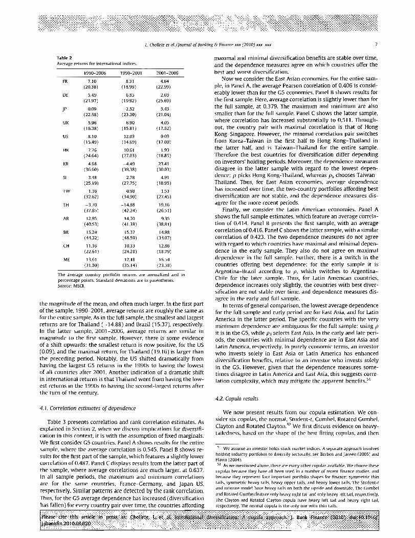
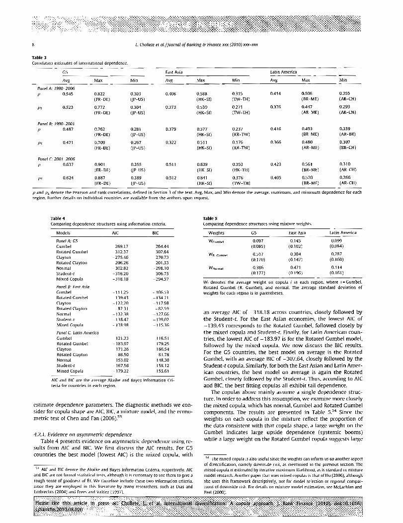
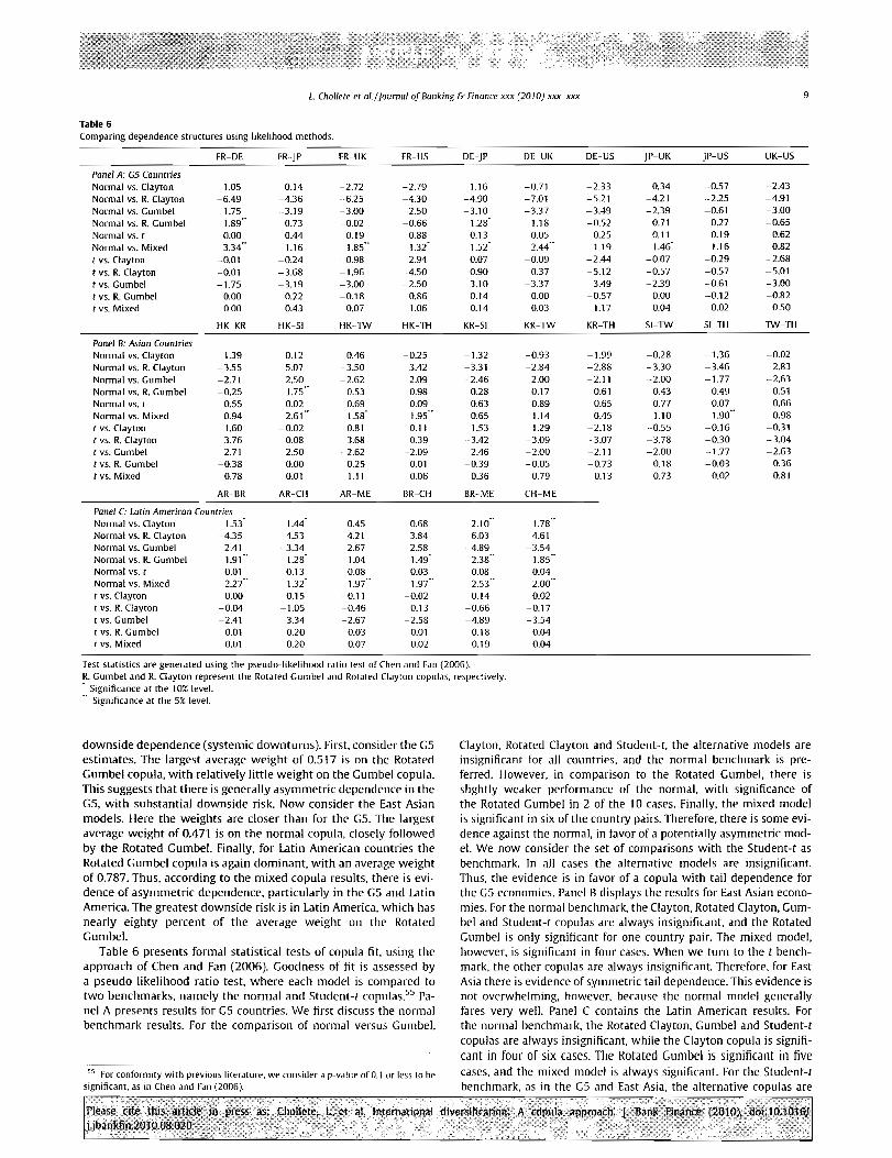
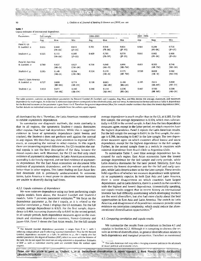
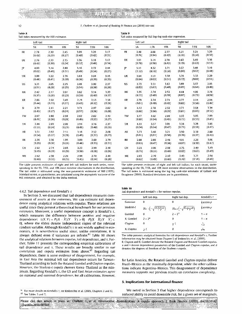
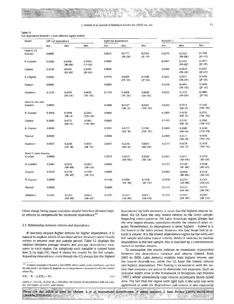
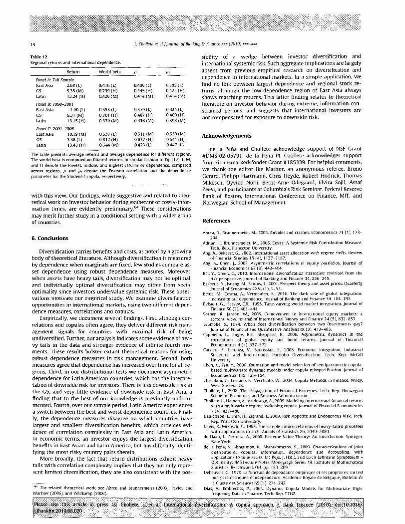
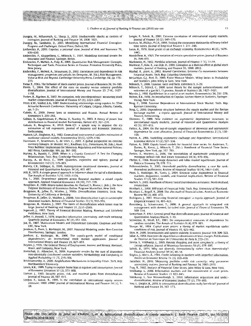


![JOURNAL OF IEEE XXX XXX, VOL. XX, NO. XX, …1103.1439v3 [cs.IT] 10 Sep 2013 JOURNAL OF IEEE XXX XXX, VOL. XX, NO. XX, AUGUST 2010 1 Generating Functional Analysis for Iterative CDMA](https://static.fdocuments.us/doc/165x107/5af78a247f8b9a9e5990dd4a/journal-of-ieee-xxx-xxx-vol-xx-no-xx-11031439v3-csit-10-sep-2013-journal.jpg)