Spatial anisotropy analyses of subcutaneous tissuelayer: potential insights into its biomechanicalcharacteristicsAndrew C. Ahn1,2 and Ted J. Kaptchuk1,2

1Martinos Center for Biomedical Imaging, Massachusetts General Hospital, Charlestown, MA, USA2Division of General Medicine and Primary Care, Beth Israel Deaconess Medical Center, Boston, MA, USA

Abstract

As the intermediate layer between the muscle and skin, the subcutaneous tissue frequently experiences shear

and lateral stresses whenever the body is in motion. However, quantifying such stresses in vivo is difficult. The

lack of such measures is partly responsible for our poor understanding of the biomechanical behaviors of subcu-

taneous tissue. In this study, we employ both ultrasound imaging and a novel spatial anisotropy measure –

incorporating Moran’s I spatial autocorrelation calculations – to investigate the structuromechanical features of

subcutaneous tissues within the extremities of 16 healthy volunteers. This approach is based on the understand-

ing that spatial anisotropy can be an effective surrogate for the summative, tensile forces experienced by bio-

logical tissue. We found that spatial anisotropy in the arm, thigh and calf was attributed to the echogenic

bands spanning the width of the ultrasound images. In both univariable and multivariable analyses, the calf

was significantly associated with greater anisotropy compared with the thigh and arm. Spatial anisotropy was

inversely related to subcutaneous thickness, and was significantly increased with longitudinally oriented probe

images compared with transversely orientated images. Maximum peaks in spatial anisotropy were frequently

observed when the longitudinally oriented ultrasound probe was swept across the extremity, suggesting that

longitudinal channels with greater tension exist in the subcutaneous layer. These results suggest that subcuta-

neous biomechanical tension is mediated by collagenous ⁄ echogenic bands, greater in the calf compared with

the thigh and arm, increased in thinner individuals, and maximal along longitudinal trajectories parallel to the

underlying muscle. Spatial anisotropy analysis of ultrasound images has yielded meaningful patterns and may

be an effective means to understand the biomechanical strain patterns within the subcutaneous tissue of the

extremities.

Key words: autocorrelation; biomechanic; mechanical; spatial anisotropy; subcutaneous tissue; ultrasound.

Introduction

Subcutaneous tissue is the adipose-rich layer under the skin

associated with a number of well-described functional roles.

It provides insulation to conserve internal body heat, acts as

a cushion to protect deeper tissue and organs, serves as an

energy and fluid reserve, and provides structural and circu-

latory support to the overlying dermis and epidermis. These

myriad functions are embodied by the complex assembly of

cells and tissues that constitute the subcutaneous layer: the

pliable and energy-rich adipocytes, the rich vascular and

neural network that support and innervate the skin, the

extensive connective tissue matrix that maintain structural

integrity, the hair follicles and sweat ducts.

A relatively unrecognized aspect of subcutaneous tissue is

its biomechanical properties. As the intermediate layer

between the muscle and skin, the subcutaneous tissue fre-

quently experiences shear and lateral stresses whenever the

body is in motion (Hermanns-Le et al. 2004). Even during

simple movements such as respiration and hand motion,

muscles and bones move laterally with respect to the skin

(Guimberteau et al. 2005). As a consequence, the subcuta-

neous tissue must be sufficiently malleable to permit uncon-

strained movement while being rigorous enough to avoid

complete untethering of the two layers. Moreover, it must

provide adequate tensile resistance to preserve the struc-

tural integrity of the nerves and vessels that traverse it.

These biomechanical characteristics are arguably integral

for the proper functioning of subcutaneous tissue yet

Correspondence

Andrew C. Ahn, MD MPH, MGH Martinos Center for Biomedical

Imaging, 149 Thirteenth Street, Room 2328, Charlestown, MA 02129,

USA. T: 617-643-6748; E: aahn1@partners.org

Accepted for publication 24 May 2011

Article published online 4 July 2011

ªª 2011 The AuthorsJournal of Anatomy ªª 2011 Anatomical Society of Great Britain and Ireland

J. Anat. (2011) 219, pp515–524 doi: 10.1111/j.1469-7580.2011.01407.x

Journal of Anatomy

remain difficult to evaluate particularly within the in vivo

setting (Gibson et al. 2006).

According to past studies, biological tissues are structur-

ally dynamic and adaptive – responding and accommodat-

ing to mechanical forces. For instance, cells such as

fibroblasts and vascular smooth muscles orient in the direc-

tion of principal strain (Kanda & Matsuda, 1994; Bischofs &

Schwarz, 2003). Collagenous networks similarly align along

the axis of tensile strain and form macroscopic asymmetries

(Girton et al. 2002; Vader et al. 2009). This structural

response to mechanical stimuli ensures that the tissue is

equipped for future, comparable forces and exemplifies the

notion that ‘structure’ follows ‘function’. For this reason,

structural properties, such as spatial anisotropy, may be an

effective surrogate for the summative, tensile forces experi-

enced by biological tissue and thereby serve as a useful

means to investigate the biomechanical behavior of sub-

cutaneous tissue (Markenscoff & Yannas, 1979). Spatial aniso-

tropy is a method to quantify the amount of preferential

orientation or alignment present in a substance or image.

In this study, we employ both ultrasound imaging and a

novel spatial anisotropy measure – incorporating Moran’s I

spatial autocorrelation calculations – to investigate the

structuromechanical features of subcutaneous tissues within

the extremities of healthy volunteers. By obtaining multiple

ultrasound images at three separate sites (arm, thigh and

calf), we investigate whether spatial anisotropies and thus

indirectly tensile strains are associated with any meaningful

anatomical patterns in vivo: do anisotropies increase with

spatial scale?; are spatial anisotropies increased at specific

extremity sites and are they related to subcutaneous layer

thickness?; and are spatial anisotropies greater in the longi-

tudinal or transverse directions (parallel or perpendicular to

the long axis of the bone, respectively)? This study seeks to

answer these questions and, in the process, obtain an

improved understanding of the biomechanical strain

patterns within the subcutaneous tissue of the extremities.

Materials and methods

Subjects and settings

Healthy participants were recruited via flyers placed throughout

Boston campus areas near Beth Israel Deaconess Medical Center

(BIDMC) and via postings in Craigslist (http://www.craigslist.org).

Subjects were excluded if they were under 18 years old, preg-

nant, had a chronic skin condition (such as eczema, psoriasis),

had a collagen disorder (scleroderma, mixed connective tissue

disorder, Marfan’s), or had a chronic medical condition requir-

ing regular medication intake. To avoid circumstances where

the complete subcutaneous layer was too thick for visualization

by the ultrasound (4 cm depth window), a body mass index

(BMI) < 30 was also required. Sixteen healthy participants were

recruited for this study. There were 11 females and five males,

with a demographic representation of 14 non-Hispanic Whites

and two Asians. Participant’s age was 29 ± 7.2 (mean ± SD)

years. Each subject was compensated for participation. The test-

ing was performed in the BIDMC General Clinical Research

Center and approved by the BIDMC Institutional Review Board.

Ultrasound image

Three specific locations were evaluated – the lateral aspect of

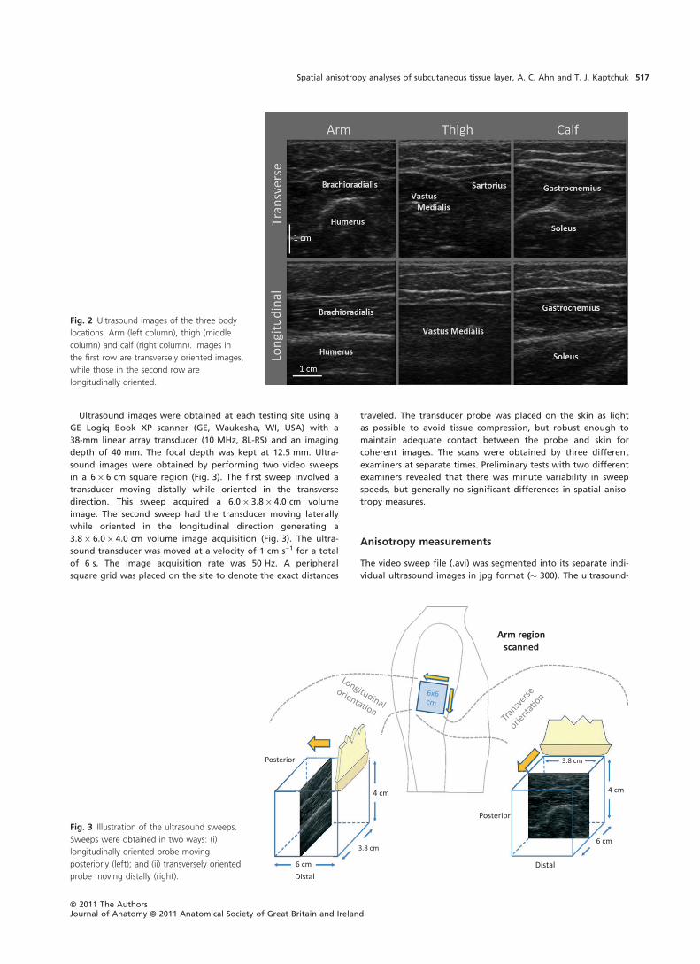
the arm, the inner aspect of the thigh and posterior calf (Fig. 1).

These sites were chosen because they were previously evaluated

in a study involving electrical impedance of subcutaneous tissue

and represented three separate segments of the extremities that

had subcutaneous layers sufficiently thick for image analyses.

The arm site was centered on the anterolateral aspect of the

upper arm between the brachioradialis and triceps at � 8 cm

above the lateral end of the cubital crease (Fig. 2, left images).

Participants laid supine on a hospital recliner in a relaxed state

with the head elevated at 30 �. The arm was kept abducted at

the shoulder � 30 �, the elbow flexed at 80 �, and the arm supi-

nated such that the palm rested flat on the lower abdominal

wall.

The site for ultrasound imaging for the thigh was centered

between the vastus medialis and sartorius muscle � 10 cm

above the medial end of the popliteal crease (Fig. 2, middle

images). During imaging of the thigh, participants laid supine

on a hospital recliner in a relaxed state. The head was elevated

at � 30 � with the arm rested to the side. To obtain optimal

imaging of the inner thigh, the hips were gently flexed during

90 � flexion of the knee and leg extroversion for maximal

comfort.

The calf site was centered on the posterior aspect of the

lower leg between the two heads of the gastrocnemius � 11 cm

below the popliteal crease (Fig. 2, right images). The participant

laid prone with the legs extended and feet plantar-flexed on

the hospital bed while the arm held a pillow at the level of the

head. The order of testing for the three sites was randomized.

Fig. 1 Body sites evaluated for this study. Lateral aspect of the arm

(upper left), medial aspect of the thigh (upper right) and posterior

aspect of the calf (bottom).

ªª 2011 The AuthorsJournal of Anatomy ªª 2011 Anatomical Society of Great Britain and Ireland

Spatial anisotropy analyses of subcutaneous tissue layer, A. C. Ahn and T. J. Kaptchuk516

Ultrasound images were obtained at each testing site using a

GE Logiq Book XP scanner (GE, Waukesha, WI, USA) with a

38-mm linear array transducer (10 MHz, 8L-RS) and an imaging

depth of 40 mm. The focal depth was kept at 12.5 mm. Ultra-

sound images were obtained by performing two video sweeps

in a 6 · 6 cm square region (Fig. 3). The first sweep involved a

transducer moving distally while oriented in the transverse

direction. This sweep acquired a 6.0 · 3.8 · 4.0 cm volume

image. The second sweep had the transducer moving laterally

while oriented in the longitudinal direction generating a

3.8 · 6.0 · 4.0 cm volume image acquisition (Fig. 3). The ultra-

sound transducer was moved at a velocity of 1 cm s)1 for a total

of 6 s. The image acquisition rate was 50 Hz. A peripheral

square grid was placed on the site to denote the exact distances

traveled. The transducer probe was placed on the skin as light

as possible to avoid tissue compression, but robust enough to

maintain adequate contact between the probe and skin for

coherent images. The scans were obtained by three different

examiners at separate times. Preliminary tests with two different

examiners revealed that there was minute variability in sweep

speeds, but generally no significant differences in spatial aniso-

tropy measures.

Anisotropy measurements

The video sweep file (.avi) was segmented into its separate indi-

vidual ultrasound images in jpg format (� 300). The ultrasound-

Fig. 3 Illustration of the ultrasound sweeps.

Sweeps were obtained in two ways: (i)

longitudinally oriented probe moving

posteriorly (left); and (ii) transversely oriented

probe moving distally (right).

Fig. 2 Ultrasound images of the three body

locations. Arm (left column), thigh (middle

column) and calf (right column). Images in

the first row are transversely oriented images,

while those in the second row are

longitudinally oriented.

ªª 2011 The AuthorsJournal of Anatomy ªª 2011 Anatomical Society of Great Britain and Ireland

Spatial anisotropy analyses of subcutaneous tissue layer, A. C. Ahn and T. J. Kaptchuk 517

generated images are calibrated in equal dimensions across

width and depth – approximately 103 pixels cm)1. The bottom

portion of each image was cropped to the level of 20 pixels

deeper than the deepest point of the epimysium in the video

sweep. The images were subsequently normalized by pixel

intensity and processed using a Moran’s I spatial autocorrelation

calculation (Moran, 1950). Moran’s I first calculates the correla-

tion between each pixel and its neighbors, and then averages

across the whole image. The calculations are represented by the

following formula:

I ¼

Pi

Pj

Wij

N

Pi

Pj

Wij zi � �zð Þ zj � �z� �

Pi

zi � �zð Þ2

where zi represents the pixel intensity of a specific locus, zj is

the intensity of its neighboring pixel, and �zrepresents the aver-

age pixel intensity of the whole image. N is the total number

of pixels within the image, while Wij is the weight matrix. The

weight matrix specifies which neighboring pixels are to be

used in the correlational analyses, and thus confers the analysis

with significant flexibility in determining the effects of

directionality and spatial separation on spatial autocorrelation

(Luna et al. 2005). For example, the horizontal spatial autocorre-

lation between neighbors distanced 5 pixels apart and within a

30 � angular window is represented by the following weight

matrix:

0 0 0 0 0 0 0 0 0 0 00 0 0 0 0 0 0 0 0 0 00 0 0 0 0 0 0 0 0 0 00 0 0 0 0 0 0 0 0 0 00 1 0 0 0 0 0 0 0 1 01 1 0 0 0 0 0 0 0 1 10 1 0 0 0 0 0 0 0 1 00 0 0 0 0 0 0 0 0 0 00 0 0 0 0 0 0 0 0 0 00 0 0 0 0 0 0 0 0 0 00 0 0 0 0 0 0 0 0 0 0

266666666666666664

377777777777777775

In nearly all ultrasound images and across all spatial scales,

the greatest spatial autocorrelation was found along the hori-

zontal (lateral) axis, while the smallest was along the vertical

axis. To derive spatial anisotropy, this study focused on the hori-

zontal and vertical axes at spatial scales (distance separation) of

1–10 pixels. Moreover, we limited our anisotropic analyses to

these cardinal axes because we were primarily interested in the

lateral stress of the subcutaneous tissue. The horizontal and

vertical spatial autocorrelations were used to derive spatial

anisotropy using the following formula:

Anisotropy ¼ eIHORIZ � eIVert

eIHORIZ þ eIVert

Maximal horizontal anisotropy had a value of +1, and

maximal vertical anisotropy had a value of )1. A value of zero

indicated the absence of any anisotropy. The global anisotropy

was obtained by calculating the anisotropy for each pixel then

averaging across the image. These calculations were performed

at separation distances of 1–10 pixels (approximately equivalent

to 0.1–1.0 mm) to investigate the effect of spatial scale on

anisotropy. The validity of the global anisotropy method was

confirmed in a set of images of varying anisotropies – including

pictures with varying numbers of horizontal and vertical lines,

with sine waves of varying wavelengths and amplitudes, and

with ultrasound images with qualitatively different amounts of

anisotropy (high vs. medium vs. low). The separation distance of

up to 1.0 mm did well in distinguishing these features, and

larger separation distances (particularly > 2.0 mm) in fact led to

more incongruent results due to prevalence of images with thin

subcutaneous layer (< 5.0 mm) and to inconsistencies in the

vertical autocorrelations. Larger spatial scales led the vertical

autocorrelation matrix to correlate structures that were not

structurally related, i.e. a collagenous band and vessel. The

1-mm cutoff was ultimately determined to be the optimal level

at which the lateral and vertical contributions to the anisotropy

were appropriately balanced given the amount of subcutaneous

tissue thicknesses. The type of image format (raw vs. jpg) had

little impact on the overall anisotropy results. Anisotropy

remained robust within levels of 0.04 for differing depths as

large as 50 pixels.

Global anisotropy was calculated for all images contained

within both the transverse and longitudinal video sweeps.

Images with imaging artifacts (e.g. shadows from air bubbles

within the gels) or blood vessels with diameters > 0.5 cm width

(thus potentially contributing to greater global anisotropy) were

excluded from analyses. These measurements were automated

with Matlab 2009b (Mathworks, Natick, MA, USA). The base

program for Moran’s I spatial autocorrelation was obtained

from Matlab Central (Hebeler, 2008) and substantially modified

for this study.

Statistical analysis

Spatial anisotropy was determined at each body site and for

spatial scales 0.2, 0.4, 0.6, 0.8 and 1.0 mm by: first taking the

average of the spatial anisotropy across each video sweep

(‘mean spatial anisotropy’); and second identifying the greatest

spatial anisotropy within each sweep (‘maximum spatial aniso-

tropy’). To determine whether spatial anisotropy was signifi-

cantly different between longitudinal and transverse

orientations at each body site and within-subject, we performed

a Wilcoxon signed-rank test for both mean and maximum

spatial anisotropy measures.

To identify factors associated with spatial anisotropy, a mixed

effects model was used to account for across-subject and

within-subject factors. The mean and maximum spatial aniso-

tropy at the spatial scale of 10 was designated as dependent

variables, while location, subcutaneous thickness and probe

orientation were entered as independent variables.

Subcutaneous thickness was obtained by averaging the dis-

tances between the lower border of the dermis and the upper

border of the epimysium images in five images equally distrib-

uted across the video sweep. The mixed effects model was con-

sidered ideal for the clustered, hierarchical data, i.e. within each

individual, there are three evaluated body sites (arm, thigh and

calf) and within each body site there are two orientations

(transverse vs. longitudinal). SAS version 9.2 software (SAS Insti-

tute, Cary, NC, USA) was used for statistical calculations.

Results

Figure 4 shows a topographic representation of anisotropy

in a sample subcutaneous layer. With increasing spatial

ªª 2011 The AuthorsJournal of Anatomy ªª 2011 Anatomical Society of Great Britain and Ireland

Spatial anisotropy analyses of subcutaneous tissue layer, A. C. Ahn and T. J. Kaptchuk518

scales, greater spatial anisotropy is seen where the echo-

genic bands are visualized in the ultrasound image. This

heightened anisotropy was particularly evident for those

bands spanning the whole width of the ultrasound image.

Global anisotropy of the subcutaneous layer generally

increased in value with greater spatial scale – maximizing at

either 0.8 or 1.0 mm depending on the body site or probe

orientation. Global anisotropy values for several sample

images are shown in Fig. 5.

As shown in Table 1a and b, the mean spatial anisotropy

(the average anisotropy across the video sweep) ranged

from 0.05 to 0.24, while the maximum spatial anisotropy

(the maximum anisotropy within the sweep) ranged from

0.06 to 0.28. No image was associated with a negative

global anisotropy, i.e. a vertical or shallow-to-deep oriented

anisotropy. In general, greater spatial scales were associated

with greater mean and maximum anisotropy; the calf

region was associated with greater anisotropies compared

with the thigh and arm; and the longitudinally oriented

images were associated with greater anisotropies compared

with transverse images. This latter observation was con-

firmed by the Wilcoxon Ranked Sum test, which showed

statistically significant differences between the longitudinal

and transverse images particularly at larger spatial scales.

These differences between the two probe orientations were

accentuated further when the maximal anisotropy values

were considered.

Multivariable statistical analyses for anisotropy at spatial

scale of 1.0 mm showed that subcutaneous thickness, body

site and probe orientation were all significantly associated

with spatial anisotropy (Table 2). Greater subcutaneous

thickness is associated with reduced mean and maximum

spatial anisotropy. After accounting for subcutaneous thick-

ness and probe orientation, the calf was associated with

greater anisotropy whereas the arm was associated with

lower anisotropy by both measures. Longitudinal probe ori-

entation is associated with greater anisotropy, particularly

for maximum spatial anisotropy.

Figure 6 demonstrates sample variances of anisotropy

across longitudinally and transversely oriented sweeps by

body site. In general, the longitudinally oriented, posteri-

orly moving sweeps generated greater variance in spatial

anisotropy than the transversely oriented, distally moving

sweeps. This variability was particularly evident at larger

spatial scales and was not limited to a single body site. In

many cases, a single peak could be seen in the longitudi-

nally oriented sweeps and frequently correlated with the

subcutaneous tissue overlying intermuscular spaces. The

peaks were defined as areas where both the 1.0 mm spatial

anisotropy and the linear slope estimates for the four larg-

est anisotropy measures (i.e. slope for the anisotropy vs.

spatial scale plot – which projects the anisotropy at even

greater scales) were at least one standard deviation above

the mean values for the full sweep. Out of 16 samples, nine

arm, seven thigh and 13 calf regional sweeps had aniso-

tropy peaks located within 2.5 mm of the intermuscular

region. The intermuscular region was defined as the loca-

tion where the intermuscular space and subcutaneous tissue

conjoined. Figure 7A–C illustrates the correlation between

images with maximal anisotropy and intermuscular fascia.

Based on a binomial distribution analysis, the probability of

having these or any greater amounts of correlations with

intermuscular fascia (� 5.0 mm thickness) within 2.5 mm of

the peak region (� 5.0 mm in thickness) in a 60-mm sweep

region is 0.05, 0.25 and < 0.001 at the arm, thigh and calf,

respectively.

Fig. 4 Topographic representation of spatial

anisotropy in a sample subcutaneous layer.

Spatial anisotropy was calculated for spatial

scales 1–10 (� 0.1 to � 1.0 mm). Only even

scales are depicted here.

ªª 2011 The AuthorsJournal of Anatomy ªª 2011 Anatomical Society of Great Britain and Ireland

Spatial anisotropy analyses of subcutaneous tissue layer, A. C. Ahn and T. J. Kaptchuk 519

Discussion

The structuromechanical properties of the subcutaneous

layer are poorly understood and have not been extensively

studied. This may partly be due to the general lack of

appreciation for subcutaneous tissue’s mechanical behavior

during physical activity and for its role in protecting its tra-

versing structures (e.g. nerve and blood vessels) from shear

and tensile forces. The lack of understanding may also be

due to the overall unavailability of techniques that can

effectively extract mechanical information about the subcu-

taneous layer, particularly within the in vivo setting.

Few animal studies, however, have provided some rele-

vant insights into subcutaneous tissue. Based on ex vivo rat

subcutaneous tissue samples under uniaxial tension, the

instantaneous elastic response of subcutaneous tissue was

found to be highly linear up to 50% strain (Iatridis et al.

2003). This is unlike other specialized connective tissues,

such as cartilage or tendons, where the elastic response is

decidedly non-linear (e.g. ever intensifying tension with

increasing strain) due to the increasing recruitment of

fibers as tensile forces rise. The linear elastic response of

subcutaneous tissue suggests that nearly most of the

structural components within the tissue are already

recruited – sensing the tensile forces within the tissue –

even at low strain levels and thus theoretically exhausted

of any extra reserve to resist additional strain. In addition,

the elastic modulus of subcutaneous tissue was � 2.75 kPa,

several orders of magnitude lower than many other solid

tissues in the body – indicating that as biological tissues go,

subcutaneous tissue is not especially stiff (Iatridis et al. 2003).

Moreover, the relatively short viscoelastic relaxation time

seen in the study revealed that subcutaneous tissue quickly

Table 1 (a) Mean spatial anisotropy and (b) maximal spatial anisotropy – role of location, orientation and spatial scale.

Location 0.2 mm 0.4 mm 0.6 mm 0.8 mm 1.0 mm

(a)

Arm

Transverse 0.053 ± 0.007 0.128 ± 0.018 0.158 ± 0.024 0.179 ± 0.028 0.180 ± 0.028

Longitudinal 0.056 ± 0.008 0.133 ± 0.022 0.165 ± 0.030 0.188 ± 0.036 0.192 ± 0.037

P-value 0.05 0.03 0.02 0.02 0.02

Thigh

Transverse 0.051 ± 0.007 0.123 ± 0.018 0.153 ± 0.024 0.176 ± 0.028 0.179 ± 0.028

Longitudinal 0.054 ± 0.009 0.129 ± 0.023 0.160 ± 0.031 0.183 ± 0.037 0.186 ± 0.038

P-value 0.004 0.005 0.02 0.03 0.04

Calf

Transverse 0.062 ± 0.008 0.153 ± 0.017 0.194 ± 0.019 0.223 ± 0.020 0.226 ± 0.020

Longitudinal 0.063 ± 0.008 0.156 ± 0.019 0.198 ± 0.022 0.231 ± 0.024 0.236 ± 0.023

P-value 0.25 0.16 0.08 0.04 0.003

(b)

Arm

Transverse 0.063 ± 0.008 0.149 ± 0.020 0.184 ± 0.028 0.208 ± 0.032 0.212 ± 0.032

Longitudinal 0.068 ± 0.010 0.164 ± 0.028 0.204 ± 0.038 0.235 ± 0.047 0.240 ± 0.046

P-value 0.004 0.005 0.006 0.006 0.008

Thigh

Transverse 0.060 ± 0.010 0.142 ± 0.025 0.177 ± 0.034 0.204 ± 0.041 0.208 ± 0.043

Longitudinal 0.065 ± 0.010 0.156 ± 0.025 0.194 ± 0.034 0.223 ± 0.042 0.228 ± 0.045

P-value 0.009 0.002 0.003 0.001 < 0.001

Calf

Transverse 0.072 ± 0.010 0.176 ± 0.022 0.221 ± 0.025 0.256 ± 0.026 0.260 ± 0.023

Longitudinal 0.075 ± 0.010 0.185 ± 0.021 0.236 ± 0.025 0.276 ± 0.029 0.284 ± 0.029

P-value 0.03 0.02 0.003 < 0.001 < 0.001

Bold text indicate variables with statistical significance (P < 0.05).

Fig. 5 Spatial anisotropy vs. spatial scale in representative samples.

ªª 2011 The AuthorsJournal of Anatomy ªª 2011 Anatomical Society of Great Britain and Ireland

Spatial anisotropy analyses of subcutaneous tissue layer, A. C. Ahn and T. J. Kaptchuk520

accommodated to each additional strain by reducing its resis-

tive tension.

Based on these findings, one would understandably con-

clude that subcutaneous tissue is simply ill-equipped to resist

any tensile ⁄ shear forces and thus mechanically incapable of

protecting the internal nerves ⁄ vessels during physical activity

or trauma. However, the rat subcutaneous tissue used in the

study is notably different from the human subcutaneous

layers analyzed in this study in one important respect: the

subcutaneous muscle of the rat ventral ⁄ lateral wall was

removed prior to the biomechanical tests. Although subcuta-

neous muscles do not typically exist in humans (except for

areas in the head, neck and hand – e.g. platysma), in our

samples, the echogenic bands within the subcutaneous layer

may act to resist tensile forces much in the way that the

subcutaneous muscle and its adjacent connective tissue

would have probably done in the rat subcutaneous sample.

Indeed, the echogenic bands were the structures highly

correlated with increased spatial anisotropy across multiple

scales, whereas areas of high adipose (and low band) content

showed no consistent change in anisotropy. Furthermore,

the spatial anisotropy at band locations frequently increased

with greater spatial scales, suggesting that the echogenic

bands operate at a macroscopic level – likely beyond the

1-mm range evaluated in this study – to resist tensile force

along the span of an extremity.

The functional significance of these echogenic bands is

presently unclear. Histologically, these bands are composed

of collagenous fibers surrounded by mucinous proteogly-

cans and glycosaminoglycans. Considering collagen’s role in

tensile resistance and the evident association between

echogenic bands and spatial anisotropy, these bands likely

Fig. 6 (a–c) Spatial anisotropy in ultrasound

sweeps. Spatial anisotropy across a 6-cm

sweep is graphed here for spatial scales 1–10

for transverse (left) and longitudinal (right)

orientations. A representative sample from

the arm (a), thigh (b) and calf (c) is shown.

ªª 2011 The AuthorsJournal of Anatomy ªª 2011 Anatomical Society of Great Britain and Ireland

Spatial anisotropy analyses of subcutaneous tissue layer, A. C. Ahn and T. J. Kaptchuk 521

provide the tensile protection to the internal structures that

is inadequately provided by the adipose tissue alone

(Knight et al. 1990). The mucinous, gel-like properties of

the neighboring glycosaminoglycan may also facilitate

sliding between collagen fibers and thereby provide the

shear plane needed for the skin to slide over muscle during

movement. Interestingly, the subcutaneous collagen of

rodents has been observed to assume this shearing role

with elastin serving the important role of maintaining

elasticity (Kawamata et al. 2003).

If indeed spatial anisotropy is correlated with the direction

and intensity of mechanical stress as we posit, this study pro-

vides some revealing insights into the mechanical behaviors

of the extremity and its subcutaneous tissue. The statistically

significant increase in longitudinal anisotropy as compared

with transverse anisotropy indicates that the subcutaneous

layer is not isolated from the mechanical stress induced by

muscle activity. At all three investigated sites, the subcutane-

ous tissue overlay muscles that effectively ran parallel to the

longitudinal axis of the extremity and thus plausibly experi-

enced greater tensile force in the longitudinal direction dur-

ing muscle contraction. Based on the ultrasound images of

the subcutaneous layer, the echogenic bands form sheets

spanning the length and circumference of the extremities.

The consistent identification of greater spatial anisotropy in

one direction was not naturally anticipated and speaks to

both the nature in which these collagenous bands are orga-

nized (much like a tablecloth crimped when two points are

tugged) and the sensitivity of our anisotropic measure.

In both our univariable and multivariable analyses, the

subcutaneous layers of the calf were significantly associated

with greater anisotropy compared with those at the thigh

and arm, whereas the subcutaneous tissue of the thigh had

greater anisotropy compared with the arm after accounting

for subcutaneous thickness and probe orientation. Based

on these results, gastrocnemius muscles may generate

greater subcutaneous stresses compared with the sartorius

and vastus medialis, while these latter muscles may gener-

ate greater biomechanical stresses compared with the bra-

chioradialis and biceps brachii. Although these anisotropy

measures do not directly assess actual, immediate muscular

stress, they may conceivably represent the composite forces

generated by the muscle over the span of the day or of

even greater periods of time. Considering the importance

of leg muscles in ambulation (a daily activity), the study’s

results are logical and consistent with this hypothesis. Nev-

ertheless, studies that directly measure muscle stress are

needed to confirm our supposition.

The inverse relationship between spatial anisotropy and

subcutaneous thickness also indicates that mechanical stress

is distributed across the subcutaneous tissue. Thicker subcuta-

neous tissues are more likely to disperse the mechanical

forces and thus are associated with reduced spatial anisot-

ropy. Thinner subcutaneous tissues, on the other hand, are

subjected to similar forces but over a smaller area. As a conse-

quence, thinner subcutaneous layers are generally associated

with greater echogenic band densities and thus spatial

anisotropy. These results may carry implications for plastic

surgeons interested in optimizing the amount of collagenous

bands in the subcutaneous tissue to reduce development of

Fig. 7 (A–C) Three-dimensional reconstructed ultrasound images of

the arm (A), thigh (B) and calf (C). Slices with maximal anisotropy are

made opaque and delineated by the gray arrows. Performed through

IMAGEJ software (version 1.44k, National Institutes of Health, Bethesda,

MD, USA).

ªª 2011 The AuthorsJournal of Anatomy ªª 2011 Anatomical Society of Great Britain and Ireland

Spatial anisotropy analyses of subcutaneous tissue layer, A. C. Ahn and T. J. Kaptchuk522

‘cellulite’ (Gasperoni & Salgarello, 1995) or for massage ther-

apists seeking to understand how manual interventions can

affect subcutaneous tissue composition in various individu-

als. Indeed, deep mechanical massage has been shown to

increase the amount of subcutaneous collagen bands in a

porcine model (Adcock et al. 2001). This corroborates the

assertion that collagenous bands are derivatives of mechani-

cal stress but must also be understood within the context that

subcutaneous thickness may significantly modify the distri-

bution of mechanical stresses and therefore greatly moder-

ate the response in band production and formation.

Based on our data, the ultrasound sweeps with longitudi-

nally oriented images were associated with greater variance

in spatial anisotropy compared with the corresponding

sweeps with transversely oriented images. Not only did maxi-

mal anisotropy measures generate greater statistical differ-

ences between the two directions when compared with the

statistical calculations using mean anisotropy, but the longi-

tudinally oriented sweeps generally revealed a visible peak in

the spatial anisotropy vs. sweep distance map. The concept

of longitudinal channels with greater mechanical stresses is

not new and has been previously proposed by manual thera-

pists. Variations on terms referring to this concept include

‘Anatomy Trains’ (Myers, 2009) or ‘Myofascial Sequences’

(Stecco, 2004), and are based on the notion that connective

tissue structures serve as an ‘ectoskeleton’ helping to mediate

force transmissions across muscles and joints (Huijing,

1999a,b, 2009; Benjamin, 2009). The fact these peaks were

significantly correlated with intermuscular spaces at the arm

and calf intimates that these fascial planes help integrate

mechanical stresses between muscles and transmit forces into

more superficial layers such as the subcutaneous tissue. The

lack of statistical significance at the thigh may be attributed

to the somewhat oblique path of the sartorius muscle and

our determination of spatial anisotropy solely along the

longitudinal axis of the extremity. This is in contrast with the

calf where the intermuscular fascia between the gastrocne-

mius muscles aligned well with the longitudinal axis of the

leg. Conceivably, calculating spatial anisotropy parallel to

the sartorius muscle would generate a more distinct correla-

tion with the intermuscular plane.

This study relied on images directly acquired from the

ultrasound device to calculate spatial anisotropy in the

subcutaneous layer. As a result, only the spatial anisotropies

in the transverse or longitudinal direction were calculated.

For future studies, computational manipulation of video

sweeps may be performed to reconfigure the images and

generate anisotropies along different axes. This study had

additional limitations. Ultrasonography inherently produces

anisotropic images because it relies on impedance of acous-

tic waves traveling from skin to deeper layers. Vertical struc-

tures (spanning from superficial to deep) poorly reflect

acoustic waves traveling in a vertical trajectory and thus are

not well characterized on ultrasound images. Spatial aniso-

tropy will nearly uniformly yield lateral anisotropies in ultra-

sonography and thus must be interpreted with this

limitation in mind. Moreover, the lateral resolution of our

ultrasound was � 0.5–1.0 mm – within the spatial range

where the autocorrelations were performed. Although this

spatial range was preliminarily tested and determined to

have construct validity, our analyses clearly depend on the

effectiveness of image processing program in interpolating

data (adding pixels in the lateral direction). Furthermore,

although no significant differences between two examiners

were identified in this study, intra- and inter-examiner

differences in ultrasound imaging acquisition must be con-

sidered as variations in ultrasound probe pressure can theo-

retically affect spatial anisotropy measures. In addition, this

study is limited by the small sample size, limited number of

body sites and its focus on the relaxed state. Future studies

should consider not only increasing the number of subjects

and body sites, but also diversifying the number of physical

positions and states assessed (e.g. tensed muscle during

flexion) to better grasp the generalizability of our findings.

Finally, as stated previously, spatial anisotropy is merely a

marker of structural tension and not a direct measure of

biomechanical force.

Despite these limitations, the spatial anisotropy tech-

nique used in this study has a number of advantages: it

is capable of determining the spatial anisotropy in any

desired direction and spatial scale given the flexibility of

the Weight matrix in the Moran’s I spatial autocorrela-

tion; it is apparently sensitive enough to detect relative

differences between images with different probe orienta-

tions and from different body sites; it is easily applied to

a widely available, non-invasive imaging technique (ultra-

sonography); and it may reflect the composite, summative

tensile behavior of the tissue considering that structures

do not likely conform to transient and infrequent forces.

As an imaging analytical technique, spatial anisotropy

has yielded some meaningful patterns, and may be a use-

ful and efficient way for evaluating the biomechanical

properties of subcutaneous layer and possibly other

tissues.

Table 2 Factors associated with mean and maximal spatial anisotropy.

Mean anisotropy Maximal anisotropy

Odds ratio P-value Odds ratio P-value

Location

Thigh (Ref) – < 0.0001 – < 0.0001

Arm 0.94 0.94

Calf 1.03 1.02

Subcutaneous

thickness (cm)

0.90 < 0.0001 0.88 < 0.0001

Orientation

Transverse (Ref) – 0.03 – 0.0002

Longitudinal 1.02 1.06

ªª 2011 The AuthorsJournal of Anatomy ªª 2011 Anatomical Society of Great Britain and Ireland

Spatial anisotropy analyses of subcutaneous tissue layer, A. C. Ahn and T. J. Kaptchuk 523

Conclusion

The application of spatial anisotropy measures to in vivo

ultrasound images has revealed various morphological

patterns within the subcutaneous tissue layer of the extrem-

ities. These patterns may provide important insights into

the biomechanical properties of the subcutaneous layer.

Although, at present, the mechanical functions of subcuta-

neous tissue remain largely unknown, this study suggests

that subcutaneous tissue is not structured in a random man-

ner and that newer techniques such as spatial anisotropy

will be important in elaborating its biomechanical role.

Acknowledgements

This research was supported by grant numbers K23-AT003238,

P30AT005895 and K24-AT004095 of the National Center for

Complementary Alternative Medicine (NCCAM), and supported

in part by a gift from The Bernard Osher Foundation. The pro-

ject described was supported by Clinical Translational Science

Award UL1RR025758 to Harvard University and Beth Israel Dea-

coness Medical Center from the National Center for Research

Resources. The content is solely the responsibility of the authors

and does not necessarily represent the official views of the

National Center for Complementary Alternative Medicine or the

National Center for Research Resources or the National Insti-

tutes of Health. The funders had no role in study design, data

collection and analysis, decision to publish, or preparation of

the manuscript.

References

Adcock D, Paulsen S, Jabour K, et al. (2001) Analysis of the

effects of deep mechanical massage in the porcine model.

Plast Reconstr Surg 108, 233–240.

Benjamin M (2009) The fascia of the limbs and back – a review.

J Anat 214, 1–18.

Bischofs IB, Schwarz US (2003) Cell organization in soft media

due to active mechanosensing. Proc Natl Acad Sci USA 100,

9274–9279.

Gasperoni C, Salgarello M (1995) Rationale of subdermal super-

ficial liposuction related to the anatomy of subcutaneous fat

and the superficial fascial system. Aesthetic Plast Surg 19,

13–20.

Gibson T, Barbanel JC, Evans JH (2006) Biomechanical concepts

and effects. J Tissue Viability 16, 24–26.

Girton TS, Barocas VH, Tranquillo RT (2002) Confined

compression of a tissue-equivalent: collagen fibril and cell

alignment in response to anisotropic strain. J Biomech Eng

124, 568–575.

Guimberteau JC, Sentucq-Rigall J, Panconi B, et al. (2005)

[Introduction to the knowledge of subcutaneous sliding

system in humans]. Ann Chir Plast Esthet 50, 19–34.

Hebeler F (2008) Moran’s I. Matlab Central.

Hermanns-Le T, Uhoda I, Smitz S, et al. (2004) Skin tensile

properties revisited during ageing. Where now, where next? J

Cosmet Dermatol 3, 35–40.

Huijing P (1999a) Muscular force transmission: a unified, dual or

multiple system? A review and some explorative experimental

results Arch Physiol Biochem 107, 292–311.

Huijing PA (1999b) Muscle as a collagen fiber reinforced

composite: a review of force transmission in muscle and

whole limb. J Biomech 32, 329–345.

Huijing PA (2009) Epimuscular myofascial force transmission: a

historical review and implications for new research.

International Society of Biomechanics Muybridge Award

Lecture, Taipei, 2007. J Biomech 42, 9–21.

Iatridis JC, Wu J, Yandow JA, et al. (2003) Subcutaneous tissue

mechanical behavior is linear and viscoelastic under uniaxial

tension. Connect Tissue Res 44, 208–217.

Kanda K, Matsuda T (1994) Mechanical stress-induced

orientation and ultrastructural change of smooth muscle cells

cultured in three-dimensional collagen lattices. Cell Transplant

3, 481–492.

Kawamata S, Ozawa J, Hashimoto M, et al. (2003) Structure of

the rat subcutaneous connective tissue in relation to its sliding

mechanism. Arch Histol Cytol 66, 273–279.

Knight KR, McCann JJ, Vanderkolk CA, et al. (1990) The

redistribution of collagen in expanded pig skin. Br J Plast Surg

43, 565–570.

Luna R, Epperson BK, Oyama K (2005) Spatial genetic structure

of two sympatric neotropical palms with contrasting life

histories. Heredity 95, 298–305.

Markenscoff X, Yannas IV (1979) On the stress-strain relation

for skin. J Biomech 12, 127–129.

Moran P (1950) Notes on continuous stochastic phenomena.

Biometrika 37, 17–23.

Myers T (2009) Anatomy Trains: Myofascial Meridians for

Manual and Movement Therapists. Philadelphia: Churchill

Livingstone.

Stecco L (2004) Fascial Manipulation for Musculoskeletal Pain.

Padova, Italy: PICCIN.

Vader D, Kabla A, Weitz D, et al. (2009) Strain-induced

alignment in collagen gels. PLoS ONE 4, e5902.

ªª 2011 The AuthorsJournal of Anatomy ªª 2011 Anatomical Society of Great Britain and Ireland

Spatial anisotropy analyses of subcutaneous tissue layer, A. C. Ahn and T. J. Kaptchuk524