Canonical quantum gravity

• Lecture 1: Introduction: The earlybeginnings (1984-1992)

• Lecture 2: Formal developments (1992-4)

• Lecture 3: Physics (1994-present)

Jorge PullinCenter for Gravitational Physics and Geometry

Penn State

Pirenopolis, Brasil, August 2000

Today’s lecture

• Spin networks: how to generate independentWilson loops

• Well defined operators: areas and volumes.

• Functional integration.

• Entropy of black holes.

In yesterday’s lecture we reviewed how a new canonical formulationof general relativity appeared to offer attractive possibilities, in particular

• The phase space was identical to that of an SO(3) Yang-Mills theory.• One could solve the Gauss law using Wilson loops.• One can introduce a representation (the loop representation) wherethe diffeomorphism constraint can be naturally handled through knotinvariants.• Promising results appeared when analyzing formal versions of thequantum Hamiltonian constraint.

We however found several aspects that need sharpening:

The calculations involving the Hamiltonian were only formal,unregulated ones. We need more experience regulating operatorsin this formalism.

The Wilson loops were an over-complete basis of functions and thatmeant that wavefunctions in the loop representations were bound bycomplicated identities.

The variables that made the Hamiltonian constraint simple were complex variables requiring us to enforce additional reality conditions to make sure we were obtaining real general relativity.

We will see how developments that happened early in the 90s helped significantly with these issues.

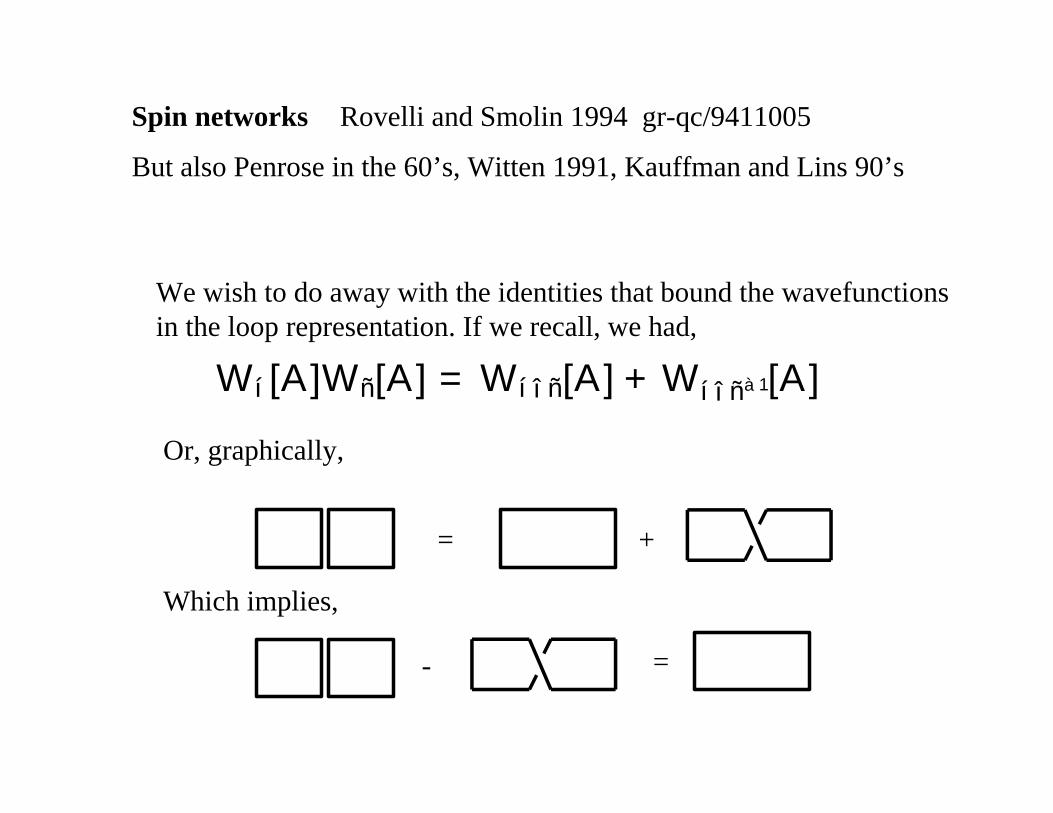
Spin networks

We wish to do away with the identities that bound the wavefunctionsin the loop representation. If we recall, we had,

Wí[A]Wñ[A] = Wíîñ[A] +Wíîñà1[A]

Or, graphically,

=

Which implies,

=

+

-

Rovelli and Smolin 1994 gr-qc/9411005

But also Penrose in the 60’s, Witten 1991, Kauffman and Lins 90’s

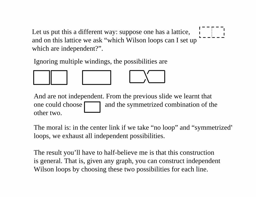
Let us put this a different way: suppose one has a lattice, and on this lattice we ask “which Wilson loops can I set upwhich are independent?”.

Ignoring multiple windings, the possibilities are

And are not independent. From the previous slide we learnt thatone could choose and the symmetrized combination of theother two.

The moral is: in the center link if we take “no loop” and “symmetrized”loops, we exhaust all independent possibilities.

The result you’ll have to half-believe me is that this construction is general. That is, given any graph, you can construct independent Wilson loops by choosing these two possibilities for each line.

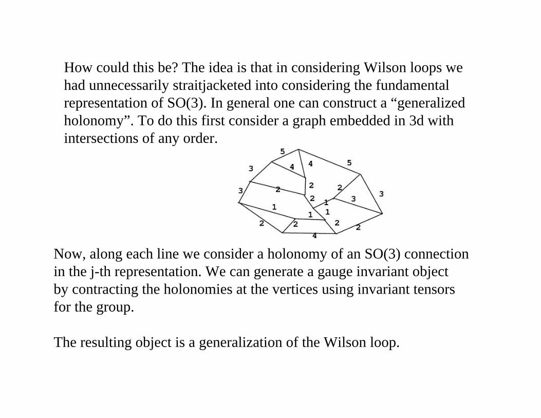
How could this be? The idea is that in considering Wilson loops wehad unnecessarily straitjacketed into considering the fundamentalrepresentation of SO(3). In general one can construct a “generalizedholonomy”. To do this first consider a graph embedded in 3d withintersections of any order.

Now, along each line we consider a holonomy of an SO(3) connectionin the j-th representation. We can generate a gauge invariant objectby contracting the holonomies at the vertices using invariant tensorsfor the group.

The resulting object is a generalization of the Wilson loop.

Considering higher order representation is tantamount to the“symmetrization” of the lines we discussed in the simple example.

Why are these objects independent? |Basically because the Mandelstamidentities come from identities of the group matrices in a given representation. They appear as a result of considering holonomiesconstrained in one representation. Therefore when one composed themone had to ensure that the resulting quantity staid in the representation.This is not the case for the objects we have, which involve lines inall possible representations.

Are spin networks different from Wilson loops? They are not. Theyare linear combinations of Wilson loops. They can simply be seen as an efficient graphical device for keeping track of which combinationsare independent. They are also very natural to work with.

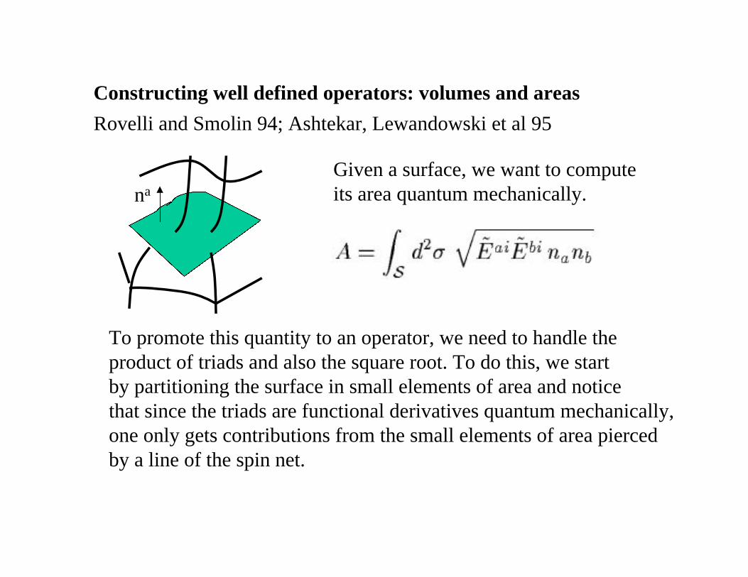
Constructing well defined operators: volumes and areas

Rovelli and Smolin 94; Ashtekar, Lewandowski et al 95

Given a surface, we want to computeits area quantum mechanically.na

To promote this quantity to an operator, we need to handle theproduct of triads and also the square root. To do this, we startby partitioning the surface in small elements of area and noticethat since the triads are functional derivatives quantum mechanically,one only gets contributions from the small elements of area piercedby a line of the spin net.

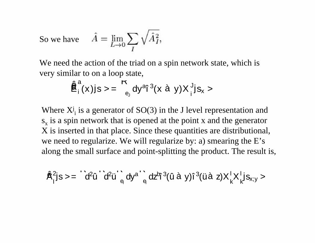
So we have

We need the action of the triad on a spin network state, which isvery similar to on a loop state,

Eàêa

i (x)js >=ReJdyaî3(x à y)XJ

ijsx >

Where Xji is a generator of SO(3) in the J level representation and

sx is a spin network that is opened at the point x and the generatorX is inserted in that place. Since these quantities are distributional,we need to regularize. We will regularize by: a) smearing the E’salong the small surface and point-splitting the product. The result is,

Aê 2

Ijs >=

Rd2ûRd2üReIdyaReIdzbî3(ûày)î3(üàz)XI

kXI

kjsx;y >

Notice that we have six one dimensional integrals and two threedimensional Dirac deltas. All these “cancel each other” and we areleft with a simple expression given by the square of the SO(3) generator in the J-th spin representation. From angular momentumtheory, we know that the value of such square is j(j+1), so theend result for the area operator is,

Aê js >=PL jL(jL+ 1)q

`2Pjs >

So we see that the area has a well defined action, and although weused background structures to regularize, the final result is topologicaland background independent. The spectrum of the operator is discrete, and admits a simple interpretation in which the spin of the lines of a spin network can be viewed as “quanta of area”.

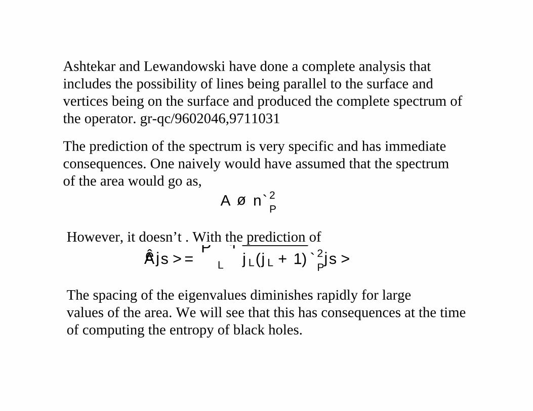
Ashtekar and Lewandowski have done a complete analysis that includes the possibility of lines being parallel to the surface and vertices being on the surface and produced the complete spectrum ofthe operator. gr-qc/9602046,9711031

The prediction of the spectrum is very specific and has immediateconsequences. One naively would have assumed that the spectrumof the area would go as,

A ø n`2P

However, it doesn’t . With the prediction of

Aê js >=PL jL(jL+ 1)q

`2Pjs >

The spacing of the eigenvalues diminishes rapidly for large values of the area. We will see that this has consequences at the timeof computing the entropy of black holes.

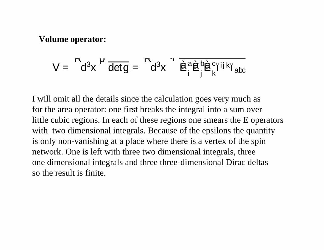
V =Rd3x detgp

=Rd3x Eà a

iEà bjEà ckïijkïabc

q

I will omit all the details since the calculation goes very much as for the area operator: one first breaks the integral into a sum overlittle cubic regions. In each of these regions one smears the E operatorswith two dimensional integrals. Because of the epsilons the quantityis only non-vanishing at a place where there is a vertex of the spinnetwork. One is left with three two dimensional integrals, threeone dimensional integrals and three three-dimensional Dirac deltasso the result is finite.

Volume operator:

The group factor is a bit more difficult to compute than before, butcorresponds to three traced generators contracted with epsilon. It can be computed. The end result is that the volume is finite, hasa discrete spectrum, and the non-vanishing contributions come from four-valent intersections or higher. The eigenvalue dependson the value of the valences that enter the intersections.

So a picture of quantum geometry emerges in which the lines offlux are associated with “quanta of area” and the intersections oflines with quanta of volume.

A measure for integration:

A key ingredient for discussing quantum physics is to have at handan inner product to compute expectation values. It is not easy to develop functional measures in infinite dimensional non-linear spaces like the space of connections modulo gauge transformations.Measures have been introduced for connections in cases like 1+1Yang-Mills, or Chern-Simons theories, but in these cases one is dealing with finite dimensional spaces.

As part of the development of the techniques for dealing with quantumgravity, mathematically rigorous measures were introduced in thesekinds of spaces, in some cases for the first time ever.

This is work due to Ashtekar, Lewandowski, Marolf, Mourao, Thiemann. Due to its heavy mathematical nature, we will only give a brief sketch here to highlight the main concepts.

(Easy to follow presentation: Ashtekar, Marolf, Mourao, Lanczos Proceedings, also in gr-qc

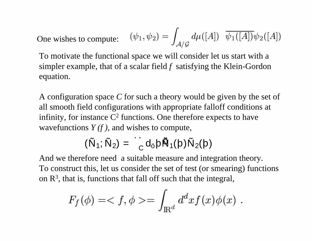
One wishes to compute:

To motivate the functional space we will consider let us start with asimpler example, that of a scalar field φ satisfying the Klein-Gordonequation.

A configuration space C for such a theory would be given by the set ofall smooth field configurations with appropriate falloff conditions atinfinity, for instance C2 functions. One therefore expects to havewavefunctions Ψ(φ), and wishes to compute,

(Ñ1;Ñ2) =RCdöþÑö 1(þ)Ñ2(þ)

And we therefore need a suitable measure and integration theory.To construct this, let us consider the set of test (or smearing) functionson R3, that is, functions that fall off such that the integral,

The functions f are called “Schwarz space” and define the simplestlinear functionals on C.

A set of functions on C one can introduce are the “cylindrical”functions. Consider a finite dimensional subspace of the Schwarzspace Vn, with a basis (e1,….,en). We can define the projections,

A cylindrical function on C is a function that depends on C onlythrough these projections,

For any function F:Rn->C

This representation is not unique. In particular any function cylindricalwith respect to Vn is cylindrical with respecto to any Vm that containsVn.

A cylindrical measure is a measure that allows to integrate cylindricalfunctions. Any measure in Rn would allow us to integrate cylindricalfunctions, but the tricky part is that there has to be consistency of thesemeasures for different choices of Vn’s.

Suppose one has Vn and Vm which have non-vanishing intersection,and with m>n, and,

Then for every cylindrical function f with respect to Vn defined by afunction F on Rn one can make it cylindrical with respect to Vm via,

And therefore one has to have that,

Any set of measures one finite dimensional spaces satisfying these conditions for any cylindrical function F, defines a cylindrical measure via,

And conversely, a cylindrical measure defines consistent sets ofmeasures in finite dimensional settings.

A particularly simple example of this construction is to consider thenormalized Gaussian measures in Rn. The resulting measure on Cis the one used in textbooks when quantizing the scalar field. TheFock space is obtained by completion of the sets of cylindricalmeasures with a certain weight.

The situation is strikingly similar to ordinary quantum mechanics,where the Hilbert space of physical states is obtained by suitablecompletions of square integrable functions on the configuration space.In field theory the situation is more involved. Not every physicalstate is a function on just the configuration space, but distributions on the time=constant hypersurface are also generically involved.

How does one generalize this to non-Abelian connections?

We introduce the notion of “hoops” (holonomic loops), that is,loops that yield the same holonomy for any connection. Suchquantities form a group (Gambini 1980’s) under composition ata given basepoint x0.

~

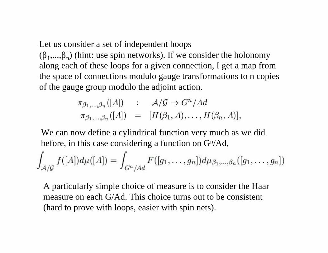
Let us consider a set of independent hoops(β1,...,βn) (hint: use spin networks). If we consider the holonomyalong each of these loops for a given connection, I get a map fromthe space of connections modulo gauge transformations to n copiesof the gauge group modulo the adjoint action.

We can now define a cylindrical function very much as we did before, in this case considering a function on Gn/Ad,

A particularly simple choice of measure is to consider the Haarmeasure on each G/Ad. This choice turns out to be consistent(hard to prove with loops, easier with spin nets).

Since the measure was defined without reference to any backgroundstructure it is naturally diffeomorphism invariant!

The construction looks intimidating but the end result is amazinglysimple, especially if one casts it in terms of spin nets. It simply statesthat

< s1js2 >=RDö[A]Ws1[A]Ws2[A] = îs1;s2

Which means that the inner product of two spin network states vanishes if the two spin network states are different. More precisely,if no representative of the diffeo-equivalence class of spin networkss1 is present in the class s2.

That is, not only have we made sense precisely of the infinite dimensional integral present in the inner product, but the result is remarkably simple at the time of doing calculations.

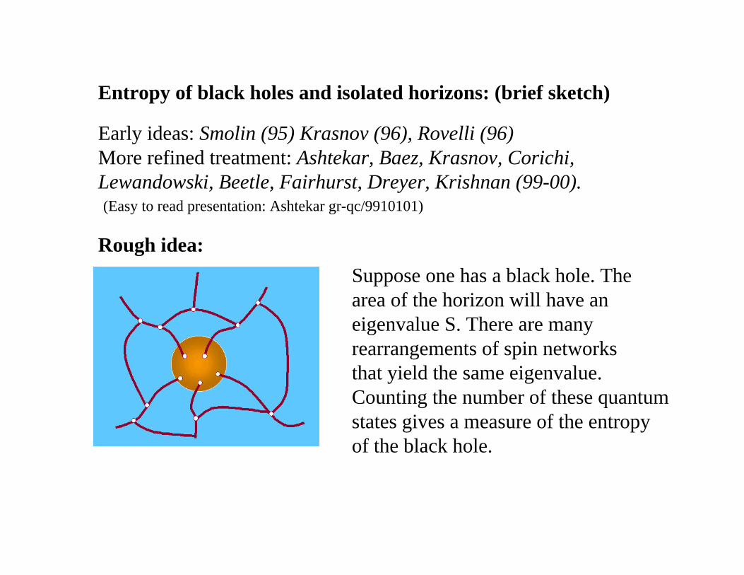
Entropy of black holes and isolated horizons: (brief sketch)

Early ideas: Smolin (95) Krasnov (96), Rovelli (96)More refined treatment: Ashtekar, Baez, Krasnov, Corichi,Lewandowski, Beetle, Fairhurst, Dreyer, Krishnan (99-00).

Rough idea:

Suppose one has a black hole. Thearea of the horizon will have aneigenvalue S. There are many rearrangements of spin networksthat yield the same eigenvalue.Counting the number of these quantumstates gives a measure of the entropyof the black hole.

(Easy to read presentation: Ashtekar gr-qc/9910101)

There are obvious problems with this proposal.

First of all, this reasoning seems to work for any area, not just thehorizon of a black hole. This might not be bad, since people speakabout a “Bekenstein bound” implying that any area would have a notion of entropy associated with our ignorance of what is inside it,the black hole case maximizing this bound.

The entropy of a black hole should be an observable. Yet, areas in general are not observables. Neither is the area of the horizon (since matter may fall in and the area grow).

How do we actually do the counting?

How does the specific dynamics of general relativity enter the calculation (it should).

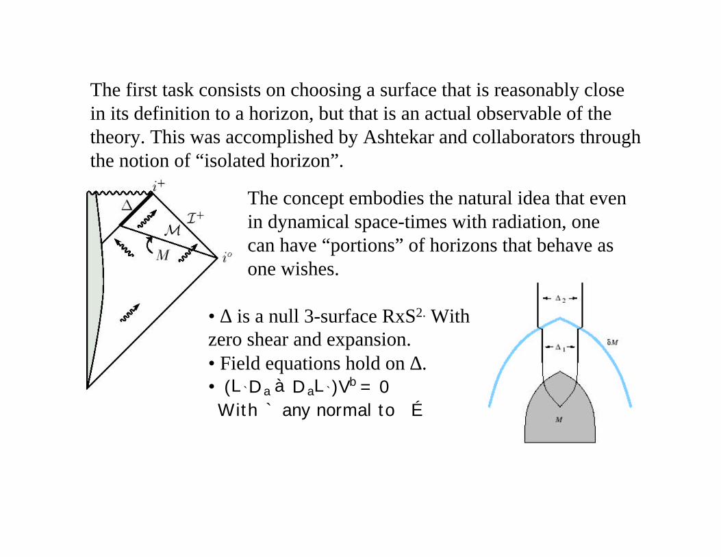
The first task consists on choosing a surface that is reasonably closein its definition to a horizon, but that is an actual observable of thetheory. This was accomplished by Ashtekar and collaborators throughthe notion of “isolated horizon”.

The concept embodies the natural idea that evenin dynamical space-times with radiation, one can have “portions” of horizons that behave asone wishes.

• ∆ is a null 3-surface RxS2. Withzero shear and expansion.• Field equations hold on ∆.• (L`Da àDaL`)Vb = 0

With ` any normal to É

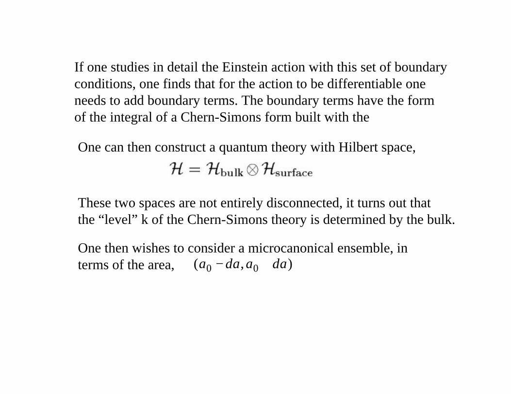
If one studies in detail the Einstein action with this set of boundaryconditions, one finds that for the action to be differentiable one needs to add boundary terms. The boundary terms have the formof the integral of a Chern-Simons form built with the

One can then construct a quantum theory with Hilbert space,

These two spaces are not entirely disconnected, it turns out thatthe “level” k of the Chern-Simons theory is determined by the bulk.

One then wishes to consider a microcanonical ensemble, interms of the area, ),( 00 aaaa δδ +−

The quantum boundary conditions dictate that for a given state in thebulk that punctures P times the surface, the Chern-Simons state hasits curvature concentrated at the punctures, one therefore has,

Each puncture adds an element of area

)1(8 +ii jjπβ and introduces a deficit

angle of value kmi /2π

Where m is in the interval [- ji ,+ji] and kis the “level” of the Chern-Simons theory.

The picture of the quantum geometry of the horizon that appears isthat it is flat except at punctures where the lines of gravitational flux“pull” the surface up and introduce curvature.

The counting of degrees of freedom on the surface is quite delicate and uses in great detail results of Chern-Simons theory that would betoo lengthy to go into detail here. The final result is:

It is good that the result (log) is proportional to the area (without the tight boundary conditions one gets results proportional to squareroot of area, for instance). The result depends on a free parameter,the Immirzi parameter (we called it β in other lectures, in the entropy literature it is usually called γ).

Considering black holes coupled to matter one notices that one getsthe correct result for the same value of the Immirzi parameter.

Similarities and differences with the stringy calculation:

• Not worked out in d>4(perhaps works in d=3)

• Bulk states end on isolatedhorizon, determine gaugefields on surface.

• Works for non-extremalholes right away.

• Has undetermined parameter

• Works in usual geometricterms

• Only partially workedout in d=4.

• Strings end on D-brane,determines gauge fields on it.

• Getting away fromextremality is hard.

• Result precisely correct.

• Uses features of string theoryto turn the calculation into amuch simpler system.

Quantum Geometry Strings

Summary:

• Significant problem in major technicalissues that plagued the formalism (andrelated ones) from the beginning.

• Spin networks provide an elegant andpowerful calculational tool

• Discreteness of areas and volumes.

• Black hole entropy: very detailedcalculation.