SIMULATIO OF THERMAL CODITIOS I TUELS AD PLATFORMS FOR

A UDERGROUD TRASPORTATIO SYSTEM 1

Jorge AMAYA, Takeshi ASAHI, Roberto ROMÁN, José A. SÁNCHEZ

Center for Mathematical Modelling (CMM), Universidad de Chile

Abstract

This document contains the thermal balance model in a metro system, by describing the basic assumptions and corresponding equations. The goal of this article is to provide the basis for the implementation of the software, which is intended to simulate a general metro line system. Based on this approach, the software can be used to study the behaviour of energy and heat exchanges inside the tunnels during operation. Some numerical simulations to illustrate the use of the tool are also included.

1 This work has been done as a part of project MODURBAN, FP6 Project: IP 516380 EC

Contract n°: TIP4-CT-2005-516380 (subproject MODENERGY, WP 16)

COTETS

1. ITRODUCTIO ......................................................................................................................... 3

2. TECHICAL DESCRIPTIO OF THE MODEL .................................................................... 5

2.1 Heat generated inside the line ................................................................................................................. 5

2.2 Heat dissipated by the trains ........................................................................................................................... 6

2.3 Heat release in the stations ............................................................................................................................. 9

2.4 Heat absorbed by the air ............................................................................................................................... 10

2.5 Heat flow absorbed by the ground ................................................................................................................ 11

2.6 Thermal balance ........................................................................................................................................... 13

2.7 Energy usage ................................................................................................................................................ 14

3. SOFTWARE DESCRIPTIO .................................................................................................... 16

3.1 Basic concepts .............................................................................................................................................. 16

3.2 Overview of the system architecture ............................................................................................................ 16

3.3 Software features .......................................................................................................................................... 16

3.4 Advantages of the system ............................................................................................................................. 16

3.5 Output interfaces........................................................................................................................................... 17

4. CASE STUDY .............................................................................................................................. 18

4.1 Weight reduction .......................................................................................................................................... 18

4.2 Improvement of the brake system RECOV .................................................................................................. 18

4.3 HVAC ........................................................................................................................................................... 18

5. COCLUSIOS .......................................................................................................................... 19

6. REFERECES ............................................................................................................................ 20

7. APPEDIX................................................................................................................................... 21

7.1 Train kinematics ........................................................................................................................................... 21

7.2 Train power calculations............................................................................................................................... 21

7.3 Inertial forces ................................................................................................................................................ 22

7.4 Rolling friction force .................................................................................................................................... 22

7.5 Aerodynamic drag ........................................................................................................................................ 22

7.6 Force due to track curve ............................................................................................................................... 23

7.7 Force due to track slope ................................................................................................................................ 23

7.8 Air flow model ............................................................................................................................................. 23

7.9 Air flow calculations .................................................................................................................................... 23

7.10 Air flow diagrams ......................................................................................................................................... 24

7.11 HVAC model ................................................................................................................................................ 25

7.12 Model inputs ................................................................................................................................................. 25

7.13 Methodology ................................................................................................................................................. 27

7.14 Simulation procedures and assumptions ....................................................................................................... 29

1. Introduction

The objective of this work is to offer a practical and affordable study tool to decrease the energy consumption of urban railways systems. The idea was to develop a working model that will predict thermal environment in:

• railway or subway cars, • trains and tunnels and • stations

This task produced the development and implementation of new software called ModEnergy, which considers Metro lines as a dynamic system. Trains move between stations and producing certain energy inputs and outputs. Therefore, we have the tunnel system that interacts with the energy exchanges that rise from the train system. Train Model:

The train was modelled as a dynamic system that moves along rails. Considering the train having a certain mass (tare weight, load and rolling inertial mass), the first step consists of defining a certain speed curve. Forces that act on the train are: inertia, rolling friction, air drag, curve and slope. From the basic equations one can calculate the required force for the train to accelerate and thus the input power as well as the energy losses.

Speed/Distance Track:

From basic kinematics, we use the speed versus distance profile for the model. A one meter interval is used, to have good enough approximations. One can input and change parameters such as: Train technology (HVAC, RECOV), mass (empty, passengers and inertia), the speed versus distance profile, operational variables (frequency, dwell time, passengers, people in stations), the power dissipated by auxiliaries, etc.

Results:

Together with the acceleration versus distance profile, one also obtains the force necessary to accelerate the train and also the different heat losses, where braking losses are included. These are presented both as Watts as well as Joules per meter. From these results it is evident that, except during braking, one important loss to the tunnel is due to Inertia. As the train moves along the track, there is power dissipated as heat being calculated as energy dissipated per track meter when a train passes. The basic idea of this approach was to have a good breakdown of the different forces that act upon the train, comparing these results with real cases of study.

The whole system of a Subway Line can be modelled as series of nodes interconnected by tracks. Each node is a station and the tracks link these stations. From a thermal and mass transfer point of view, all nodes are linked. Usually, air enters through stations, flows along corridors, platforms and tunnels, to be evacuated at draught shafts inside the tunnel. Air gains heat and moisture, from waste heat in the system and moisture released by passengers and other water sources. The goal is to measure the energy released by the trains and to estimate how this energy is related to operation procedures, ambient conditions, trains technology, track profiles, etc.

The Energy Balance Model was constructed to evaluate the “Heat Transfer” inside the tunnel, taking place between the surrounding soil, inside air and inner loads. Assuming average peak loads and normal train running conditions, the line divided in several control volumes where the following loads are considered: Train: is a thermal energy source. This energy comes from rolling and air friction, braking losses, auxiliary power dissipated into the tunnel and passenger thermal load. The train movement also contributes to the total tunnel air flow by its piston effect. Air in tunnel: it heats up in response to the thermal energy dissipated by successive trains. It is also a heat sink as it is evacuated from the tunnel. Earth around the tunnel and stations: this is a thermal sink, since it can absorb energy from the air.

Figure: Energy balance model through the line

For the developed model, heat loads of the train, air inside the tunnel, earth around the tunnel stations, passengers and other machinery, such as HEVACs, were interrelated by means of heat transfer equations. Different time-dependent equations were aggregated and discretised in order to establish the thermal equilibrium for each hour along a day. Based on the developed model, the software called ModEnergy was developed in order to make the corresponding calculations.

2. Technical description of the model

In each control volume, the following balance takes place:

GAL Q+Q=Q &&& (1)

Q̇L = Heat flow generated inside the line, in [W] Q̇A = Heat flow absorbed by the air, in [W] Q̇G = Heat flow absorbed by the ground, in [W] S i = Start station, for a train running from a Left to Right parameterization

1+iS = Next station for a train running from a Left to Right parameterization After some standard calculations, we can achieve the differential equation which governs the temperature evolution inside each control volume.

( ) ( ) ( ) ( )[ ]iiWE,i

i

i

i

iiL zt,Tzt,Tzt,H+

z

TCpm+

t

TCpm=zt,

t

Q−

∂

∂

∂

∂

∂

∂& (2)

Where:

Q̇L = ( )iL zt,

t

Q

∂∂

Q̇A = z

TCpm+

t

TCpm i

ii

i ∂∂

∂∂

&

Q̇G = ( ) ( ) ( )[ ]iiWE,i zt,Tzt,Tzt,H −

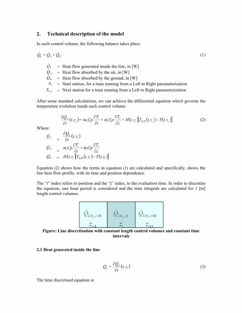
Equation (2) shows how the terms in equation (1) are calculated and specifically, shows the line heat flow profile, with its time and position dependence. The “i” index refers to position and the “j” index, to the evaluation time. In order to discretise the equation, one hour period is considered and the time integrals are calculated for 1 [m] length control volumes.

Figure: Line discretisation with constant length control volumes and constant time

intervals

2.1 Heat generated inside the line

( )iL

L zt,t

Q=Q

∂∂

& (3)

The time discretised equation is:

( ) ( ) ( )jiL,

j

jiL,jiL,

j

iL

j

t∆Q∆t

=tQtQ∆t

=dtzt,t

Q

∆t

1)()(

111−−

∂∂∫ (4)

( )izt,t

Q

∂∂

= Line heat time partial derivate, a function of time and position through the z-axis, in [W]

( )ji t∆Q = Heat release in each control volume through the evaluation period, in [J]

As the time intervals are constant and also the control volumes lengths, the only parameter needed is the total thermal amount dissipated in each control volume during this period, to obtain the mean heat flow. This depends on how many trains pass during the given time interval, the type of train, its speed, the number of transported passengers, stations technology, etc. The heat profile release inside the line will be:

iS,iT,iL, Q+Q=Q (5)

QT , i = Heat dissipated by the trains in each control volume, in [J] Q S ,i = Heat carried to, and generated in stations in each control volume, in [J]

2.2 Heat dissipated by the trains

A train along a track section has a distinct speed versus distance profile, depending on the trajectory of the train, which is defined by the system operator. This input and the track profile are the base, from where the kinematics and the energy consumption of the train are calculated2. To calculate the heat release by the trains during this hour, mean operation values are used3, in order to have, for each travelling direction, a single heat profile over a line section (

iT,Q ).

With this consideration, the total heat amount, release by the trains, will be this value multiplied by the train’s frequency, as shown below.

RL

iT,RL

LR

iT,LRiT, Qf+Qf=Q ⋅⋅ (6)

f LR = Train frequency for the Left-Right direction, in trains/hour. LR

iT,Q = Heat dissipated by the trains running in the Left-Right direction in the “i” control volume during the evaluation period, in [J]

f RL = Train frequency for the Right-Left direction, in trains/hour. RL

iT,Q = Heat dissipated by the trains running in the Right-Left direction in the “i” control volume during the evaluation period, in [J]

The heat generated by a train can be split in four terms, according to its acceleration rate, the use of brakes, friction losses and constant heat values related with the passenger load and the use of auxiliaries.

2 See Appendix 3 Average number of passengers inside the train

Equation (7) shows the train different heat sources.

D

iT,

B

iT,

AP,

iT,

F

iT,iT, Q+Q+Q+Q=Q (7)

F

iT,Q = Train friction losses, in [J] AP,

iT,Q = Heat flow release by the train because of passengers and auxiliary equipment, in [J]

B

iT,Q = Train braking losses, in [J] D

iT,Q = Train drive losses, in [J]

Friction losses

This term considers friction from wheels to rails or train to air. The amount of energy dissipated on friction is calculated as the power wasted due to Aerodynamic Drag Forces and Curve Forces, plus the Rolling Friction Force work4.

( ) ( )[ ] iiiR,iC,iD,

F

iT, tzVF+F+F=Q δ⋅ (8)

F D ,i = Aerodynamic drag force, in [N] F C , i = Curve force, in [N] F R ,i = Rolling friction force, in [N] ( )izV = Train speed at the zi segment, in [m/s]

itδ = Time used by the train to go through the control volume, in [s]

Passenger & auxiliary losses

The second term considers the heat generated by electrical auxiliaries (lights, ventilators, cooling systems, etc.) and passengers. The trains are modelled as a car array system, since each car has its own technology, passenger capacity, surface, etc. Properties that are evaluated when it comes to calculate the cars heat to tunnel flow. In the Appendix the HVAC model is described, basically in order to calculate the cooling power needed to maintain the selected comfort temperature and evaluate all the heat sources in the car. These loads are: the Passenger Load, the Air Load (heat exchange with the outside air by air renovation and HVAC system) and the Conduction Load. The heat flow release by each car, and thus a train with “n” cars, will be:

i

n

=k

HVAC

kCar,

Aux

kCar,

Cond

kCar,

Pass

kCar,

AP,

iT, tQCOP

+Q+Q+Q=Q δ⋅

∑1

1&&&& (9)

Pass

kCar,Q& = Car k, passenger sensible and latent heat flow, in [W] Cond

kCar,Q& = Car k, conduction load, in [W] Aux

kCar,Q& = Car k, auxiliary power, in [W]

4 See Appendix

HVAC

kCar,Q& = Car k, cooling power needed to maintain comfort conditions, in [W]

COP = HVAC’s coefficient of performance.

Passenger sensible and latent heat

A constant value is used when it comes to evaluate the latent and sensible heat dissipated by the passengers in each car.

kCar,s

Pass

kCar, PassH=Q ⋅& (10)

kcar,Pass = Number of passengers in the “k” car

sH = Human sensible and latent heat standing, set as 110 [W]

Conduction load

Heat exchange with the outside, through the car’s surface.

[ ]ComforttunnelkCar,kCar,

Cond

kcar, TTAk=Q −~& (11)

kCar,k = Overall car conduction heat transfer coefficient, in [W/(m2K)]

ACar , k = Car surface area, in [m2]

tunnelT~

= Tunnel air mean temperature, in [ºC]

ComfortT = Train inner comfort temperature, in [ºC]

Auxiliary power

According with the car technology their auxiliaries are considered as an input and could be split into: pneumatic systems, lightning systems, security systems, etc. Cooling power

The necessary Cooling power to maintain comfort conditions inside each car is calculated from the HVAC model.

Braking losses

As the train brakes one part of the energy needed to decrease its speed is re-injected to the lines and the other part is dissipated as heat. Heat dissipated in the breaking phase can be calculated as:

| | ( )[ ]( )RECOVQ∆E+∆E=Q F

iT,iP,ik,

B

iT, −− 1 (12)

ik,∆E = Train kinetic energy difference through the control volume, in [J]

iP,∆E = Train potential energy difference through the control volume, in [J]

RECOV = Braking recovery rate, 0,750 ≤≤ RECOV

Drive losses

Electric and mechanical inefficiencies are taking into account as the train increases its acceleration. D

iT,Q is the energy loss related with the differences between the drive electrical

power consumption and the mechanical power necessary for motion5.

δtPPη

=QMech

iT,

Mech

iT,

D

iT, ⋅

−

1 (13)

Mech

iT,P = Train mechanical power needed to overcome all the forces against its motion at speed ( )izV , in [W]

η = Train traction chain efficiency, 10 ≤≤ η

2.3 Heat release in the stations

In each station, besides the heat release by the trains at the departure and at the arriving of them, other heat sources are present. Sources like the heat carried by the air from outside, the amount of people circulating in the station and the auxiliaries required for them. Therefore, the heat release in the stations ( SQ ) can be written as:

[ ] dwell

Sj

People

S

Air

S

Aux

SS Q+∆tQ+Q+Q=Q ⋅&&& (14)

Aux

SP = Station auxiliary power, in [W] Air

SQ& = Station fresh air heat flow, in [W] People

SQ& = Sensible and latent loads release by the people in the station, in [W] dwell

SQ = Heat release by the trains during its station dwell time, in [J]

Station auxiliary power

It is assumed that the station total electrical auxiliary input is release as heat. The Station Auxiliary power is modelled as a function of the average amount of people inside of it and, minimum and maximum power capabilities.

( ) ( ) ( )( ) )exp1( / τPAux

S

Aux

S

Aux

S

Aux

SSminPmaxP+minP=Q

−−−& (15)

Aux

SP = Station electrical auxiliary power, in [W]

( )maxP Aux

S = Station maximum electrical auxiliary power, in [W]

( )minPAux

S = Station minimum electrical auxiliary power, in [W]

SP = Average number of people in the station

τ = Number of people needed to used a 63% of the station maximal electrical power

5 See Appendix

Station fresh air heat flow

The outside air conditions are fundamental in the stations inner energy balance, because it’s from this point where they influence the whole line. But not only fresh air is brought to the station, also air from the previous section leaks in to the Station. As the air flow rate must keep constant (not mass gaining are allowed), an arbitrary parameter is introduce to measure how much new air came to the station and how much air came from the previous section. The air load is:

[ ]( )SoutAp,S

Air

S TTCmγ=Q~

−&& (16)

Ap,C = Air specific heat, in [J/(kgK)]

Sm& = Station air mass flow, in [kg/s]

outT = Outside air ambient temperature, in [ºC]

ST~

= Station air mean temperature, in [ºC]

Sensible and latent loads release by the people in the station

The heat dissipated by the people in the stations is hard to evaluate, mostly because of the people’s flow inaccuracy and their chaotic behaviour. However, a simple approach has been taken, with the average amount of people in the station, for our given time interval.

Sw

People

S PH=Q ⋅& (17)

SP = Average number of people in the station

wH = Human load walking, in [W]

Heat release by the trains during its station dwell time

The trains have a particular dwell time according to the station and their direction. ( )AP,

RLT,

Dwell

RLRL

AP,

LRT,

Dwell

LRLR

dwell

S Qtf+Qtf=Q ⋅⋅⋅⋅ (18)

dwell

LRt = Trains dwell time at the station LR direction platform, in [s] dwell

RLt = Trains dwell time at the station RL direction platform, in [s]

2.4 Heat absorbed by the air

z

TCpm+

t

TCpm=Q i

ii

iA ∂∂

∂∂

&& (19)

Mean heat values are obtained when equation (19) is integrated through the operational period. The first part of the equation refers to the energy stored in the control volume air mass:

( ) ( ) ( ) ( ) ( )[ ]1

~~~11−−≈

∂

∂∫ jijiji

j

ii

i

j

tTtTCptm∆t

dtzt,t

TCptm

∆t (20)

( )ji tm~ = Mean mass of the control volume bulk air, for the t j operational

period, in [kg/s]

( )ji tT

~ = Control volume bulk air mean temperature, for the actual operational

period, in [ºC]

( )1

~−ji tT = Control volume bulk air mean temperature, for the previous operational

period, in [ºC] The second part is related with the heat carried by the air flow. Two distinct air flows are modelled ( )iRL,iLR, m+m && . Each one of them takes into account the influence of relative air

movement6.

( ) ( )( ) ( ) ( ) ( )

∆

−+

∆

−≈

∂

∂ +−

∫i

jiji

iRL

i

jiji

iLRi

i

i

j z

tTtTm

z

tTtTmCpdtzt,

z

TCptm

∆t

1,

1,

~~~~1

&&& (21)

iLR,m& = Air mass flow through the “i” control volume, in the LR direction, in [kg/s]

iRL,m& = Air mass flow through the “i” control volume, in the RL direction, in [kg/s]

( )ji tT 1

~− = Previous control volume mean bulk air temperature, for the actual

operational period, in [ºC]

( )j+i tT 1

~ = Next control volume mean bulk air temperature, for the actual

operational period, in [ºC] Finally, as the control volumes have constant length [ ]i∆z equal to one meter, equation (21)

can be written as:

( ) ( ) ( ) ( )( ) ( ) ( )( )[ ]j+ijiiRL,jijiiLR,ii

i

j

tTtTm+tTtTmCpdtzt,z

TCptm

∆t11

~~~~1−−≈

∂∂

−∫ &&& (22)

2.5 Heat flow absorbed by the ground

( ) ( ) ( )[ ]iWE,iiG zt,Tzt,Tzt,H=Q −& (23)

( )izt,H = Global heat transfer coefficient between the air and the wall, in (zi) the segment and in the (t) instant , in [W/K]

( )iWE, zt,T = Wall temperature in the (zi) segment and in the (t) instant, in [ºC]

( )izt,T = Control volume bulk air temperature in the (zi) segment and in the (t) instant, in [ºC]

Earth temperature at the wall of the tunnel depends firstly on the heat transfer from earth surface to deeper layers. Secondly, the air in the tunnel itself influences the earth temperature at the tunnel wall.

6 The air flow model is included in the Appendix

The calculations are based on approximations for the earth temperature which varies with the season of the year and depth under surface. Heat transfer coefficients for the heat flow between air, tunnel wall and earth are estimated from material coefficients, flow properties and geometric parameters. This part is modelled like an earth heat exchanger with the following assumptions:

• Homogeneous earth is situated above and around the tunnel • Ground properties are constant

To calculate the heat exchange in the tunnel, the total length of the tunnel is divided into segments which are treated step by step. Each segment is supposed to carry air of constant temperature so that heat exchange in the segment leads to a jump in temperature at the border between two segments. The heat exchange for each segment is:

( )WE,iLiG TTU∆z=Q −& (24)

i∆z = Length of the segment, = 1[m]

LU = Heat transfer factor per length of wall between bulk air and wall, in [W/(m2K)]

WE,T = Earth temperature at the wall of the tunnel, in [ºC]

iT = Air bulk temperature, in [ºC]

It is necessary to introduce a correction factor to represent the influence of the tunnel on the earth temperature. Then, comparing the heat flow from the earth surface to the tunnel with the heat flow through the tunnel wall the corrected earth temperature at the wall of the tunnel is:

1*

,0*

+U

T+TU=T

iE

WE, (25)

Where U* is the conductance ratio of heat transfer from earth surface to tunnel and from airflow to tunnel wall. This parameter U* is defined to take into account thermal conductivity of the earth, heat transfer coefficient between the airflow and the earth at the tunnel wall as well as the geometric configuration:

( )

−1//ln

122

0000

*

RS+RSU

πλ=U

L

(26)

λ = ground thermal conductivity, in [W/(mK)]

0S = depth of tunnel centre under surface, in [m]

0R = hydraulic radius of tunnel, in [m]

The heat transfer coefficient per length of wall of tunnel (UL) depends only on (hi), the heat transfer coefficient at the inner surface of the tunnel, in the form:

iL hπR=U 02 (27) The heat transfer coefficient at the inner surface of the tunnel (hi) depends on flow properties, dimensions of the tunnel and material properties of the air in the tunnel:

02R

4uλ=h TA,

i (28)

TA,λ = Air thermal conductivity, in [W/(mK)]

The Nusselt number (Nu) of air in a tunnel depends on Reynolds number (Re) and thus on flow rate. For turbulent airflow Gnielinski proposes the following approximation:

( ) 0.40.8 1000.0214 reu PR=4 − (29)

u4 = Prandtl number

eR = Reynold number

The earth temperature at the wall of the tunnel not influenced by the tunnel (TE,0) is calculated from the ambient air temperature with its mean value (Tm) and its maximum value (Tmax), assuming a sinusoidal temperature variation throughout the year.

( ) ( )ξAeTTT=T s

ξ

mmaxmE −−− − cos,0 (30)

A parameter ξ describes the “thermal depth” of the tunnel. Heat flows from air to earth surface without resistance.

λt

πρS=ξ c

00 (31)

SA = Season constant (=0 for summer and =0.5 for winter).

0t = Duration of year, in [s] (1 year=31,5 106[s])

cρ = Volumetric heat capacity of ground, in [J/(m3K)]

Finally the time discrete equation, and thus the heat absorbed by the surrounding ground, is:

( ) ( ) ( )[ ] ( ) ( )[ ]jEjiL

iiWE,i

j

tTtT+U

UU=dtzt,Tzt,Tzt,H

∆t,0*

* ~

1

1−−∫ (32)

2.6 Thermal balance

The energy balance model shows how all the energy inputs are calculated, from that point, we create a homogenize heat flow balance, just dividing by the operational period duration, which in this case is 3600 seconds.

( ) ( ) ( ) ( )[ ]

( )1,0*

*

11*

*

~

1

~~~

1

−

−−

ji

j

EL

j

L

j+iiRL,jiiLR,ji

j

LRLLR

tT∆t

mCp+T

+U

UU+

∆t

Q=

tTm+tTmCptT∆t

mCp+

+U

UU+Cpm+m &&&&

(33)

Equation (34) is the matrix view of the problem, where the x vector represents the tunnel temperature profile.

Q=T & H (34) Equation (33) could also be simplified and written as:

[ ] )(~

)(~

)(~

)(~

)(~

)(~

1,,,1,1, −+− ++=⋅+⋅−⋅ jiAjiGjiLjiiRLjiiLRji

total

i tQtQtQtTHtTHtTH&&&

(35)

total

iH =

iprevTiwalliRLiLR HHHH ,,,, +++ is the Total heat transfer ratio, in [W/K]

iLRH , = iLR,mCp & , Total heat transfer ratio from Left to Right, in [W/K]

iRLH , = iRL,mCp & , Total heat transfer ratio from Right to Left, in [W/K]

iwallH , =

1*

*

+U

UU L , Heat transfer due to wall heat flow absorbed in the “i” control

volume, in [W]

iprevTH , =

j∆t

mCp, Previous average bulk air heat flow release in the “i” control volume,

in [W]

)(~

, jiL tQ& = Actual average line heat flow release in the “i” control volume, in [W]

)(~

, jiG tQ&

= ,0EwallTH actual average wall heat flow absorbed in the “i” control volume, in

[W]

)(~

1, −jiA tQ&

= ( )1

~−jiprevT tTH Previous average bulk air heat flow release in the “i” control

volume, in [W] This equation shows the real effect of each of the variables involved in the energy balance. From here we observe that the tunnel lining and surrounding ground have a large thermal mass and are strongly coupled to the air within the system. From equation (33) the air bulk temperature is calculated.

2.7 Energy usage

If we consider the traction chain efficiency η , as a constant, the power needed by the drive

system Drive

iT,P is only a function of the mechanical power and thus, function of the forces

against its motion.

Mech

iT,

Drive

iT, Pη

=P1

(36)

The total energy usage will came from the motion power and the one used in auxiliaries, but with the caution, of taking into account the energy recovered in the braking phase ER.

[ ] ii

Aux

iT,

Drive

iT,iT, ERδtP+P=E − (37)

iT,E = Train energy usage, in [J] Drive

iT,P = Drive power required by the train, in [W] Aux

iT,P = Auxiliary power required by the train, in [W]

iER = Energy recovered in the breaking phase, in [J]

In order to have a better view of which forces contribute in a mayor way or have more relative weight, in the train drive power needed to achieve the desired speed, an energy breakdown equation display is generated.

ERE+E+E+E+E+E=E Aux

iT,

S

iT,

C

iT,

D

iT,

R

iT,

I

iT,iT, − (38)

I

iT,E = Drive needed energy to overcome the inertial force, in [J] R

iT,E = Drive needed energy to overcome the rolling friction force, in [J] D

iT,E = Drive needed energy to overcome the air drag force, in [J] C

iT,E = Drive needed energy to overcome the curve force, in [J] S

iT,E = Drive Needed energy to overcome the slope force, in [J] Aux

iT,E = Auxiliary energy consumption, in [J]

3. Software description

3.1 Basic concepts

ModEnergy is powerful and easyand was conceived to be used in “what A fundamental difference between this that the simulators are normally calculating on the base of time steps, mostly also in constant time-steps of 1second. This tool is

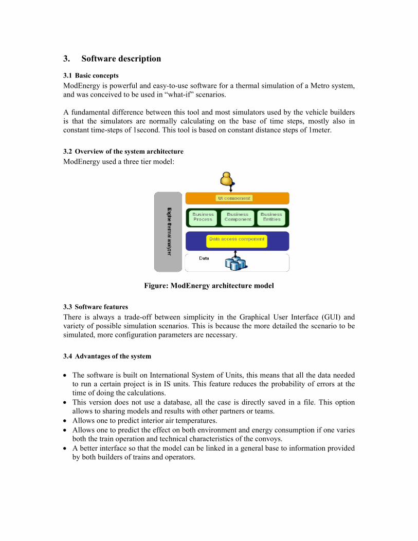
3.2 Overview of the system architecture

ModEnergy used a three tier model:

Figure: ModEnergy architecture model

3.3 Software features

There is always a trade-off between simplicity in the Graphical User Interface (GUI) and variety of possible simulation scenarios. This is because the more detailed the scenario to be simulated, more configuration parameters are necessary.

3.4 Advantages of the system

• The software is built on International System of Units, this means th

to run a certain project is in IS units. This time of doing the calculations.

• This version does not use a database, all the allows to sharing models and resu

• Allows one to predict interior air temperatures.• Allows one to predict the effect on both environment and energy con

both the train operation and technical characteristics of the convoys.• A better interface so that the model can be linked in a general base to information provided

by both builders of trains and operators.

ModEnergy is powerful and easy-to-use software for a thermal simulation of a Metro system, and was conceived to be used in “what-if” scenarios.

A fundamental difference between this tool and most simulators used by the vehicle builders is that the simulators are normally calculating on the base of time steps, mostly also in

This tool is based on constant distance steps of 1m

rchitecture

ModEnergy used a three tier model:

Figure: ModEnergy architecture model

off between simplicity in the Graphical User Interface (GUI) and possible simulation scenarios. This is because the more detailed the scenario to be

simulated, more configuration parameters are necessary.

The software is built on International System of Units, this means that all the data neecertain project is in IS units. This feature reduces the probability of errors at the

time of doing the calculations. This version does not use a database, all the case is directly saved in a file. This option allows to sharing models and results with other partners or teams. Allows one to predict interior air temperatures. Allows one to predict the effect on both environment and energy consumption if one varies

train operation and technical characteristics of the convoys. erface so that the model can be linked in a general base to information provided

by both builders of trains and operators.

use software for a thermal simulation of a Metro system,

simulators used by the vehicle builders is that the simulators are normally calculating on the base of time steps, mostly also in

distance steps of 1meter.

off between simplicity in the Graphical User Interface (GUI) and possible simulation scenarios. This is because the more detailed the scenario to be

at all the data needed reduces the probability of errors at the

directly saved in a file. This option

sumption if one varies

erface so that the model can be linked in a general base to information provided

3.5 Output interfaces

The first and most valuable result is the calculation matrix generated for a single train moving between two certain stations forward or backward, according with the operational period. As we use control volumes we have all the data for each meter. The calculation matrix results are: • time (s) • Speed (km/h) • distance (m) • acceleration (acc) (m/s2) • Kinetic Energy (J) • Potential Energy (J) • Energy (J) • Inertial Force (N) • Rolling Friction Force (N) • Aerodynamic Drag Force (N) • Curve Force (N) • Slope Force (N) • Mechanical Power (W) • Curve Losses (J) • Drag Losses (J) • Rolling Friction Thermal Losses (J) • Friction Losses Thermal (J) • Passenger & Aux Losses Thermal (J) • Braking Thermal Losses (J) • Electric Motors Thermal Losses (J) • Heat dissipated by the train or Train heat(J) • Inertial Force Contribution in the Electric Energy Consumption (J) • Rolling Friction Contribution in the Electric Energy Consumption (J) • Aerodynamic Drag Force Contribution in the Electric Energy Consumption (J)) • Curve Force Contribution in the Electric Energy Consumption (J) • Slope Force Contribution in the Electric Energy Consumption (J) • RECOV Contribution in the Electric Energy Consumption (J) • Amount of Electric Energy used by the Train Motors or Energy Drive (J) • Aux Contribution in the Electric Energy Consumption (J) • Total amount of Electric Energy used by the Train or Energy Usage (J) • Tractive Effort (kN) • Brake Effort (kN) • Energy Drive (kWh) • Moving Resistance (kN) Once it is calculated the software offers the possibility of plotting the different results against distance or time. Two main tabs may be accessed, one involving the energy usage in each train, and the other concerning the temperature evolution of the different sections.

4. Case study

Factors influencing the consumption of operation energy of trains include the performance of train traction and braking, weight of the train, HVAC set point, and the operational parameters. The operation energy for trains can be saved by making alteration to the relevant conditions. We focus on the influence of the previous conditions on the energy conservation of two Metro systems using case design and the software simulation. Two real lines were studied. For this exercise, each line segment was constructed with 3 stations. Concerning ambient conditions, all the simulations were performed on an average summer day.

4.1 Weight reduction

How the train tare mass affects its energy consumption and the heat released by it.

4.2 Improvement of the brake system RECOV7

Electrical re-injection of braking energy into the system in practice signifies an energy savings of not around 25%.

4.3 HVAC

Two parameters were separately contrasted. The car’s inner comfort temperature8 and the HVAC coefficient of performance (COP). Each new characteristic was evaluated through a whole operational day. The HVAC’s set point temperature was increased from 19 to 31 ºC. In our model a COP equal to 1 means that no HVAC system is present, therefore the lowest COP value was set as 1.001 for an inefficient HVAC system.

7 Braking Energy Recovery Rate 8 As ssuggested in the European Standard Norms NF EN 14750-1

5. Conclusions

� RECOV is only recommended when wayside energy storage is available.

� The HVAC’s set point temperature is important only at places where not extreme environment conditions are present. Under these conditions the set point temperature must be as high as possible in warm seasons and as low as possible during cold seasons. HVAC’s Cop must be as high as possible.

� On cooling mode, currently there are not many technological solutions to be applied in

order to have a clear energy factor advantage. Better efficiency and COPs values could be obtained with steeples control capacity systems, as frequency variation systems, but this will imply a big economical impact on the HVAC system, with no reduction effect on the other train systems.

� On heating mode, the application of Heat Pump technology will be an effective solution to

reduce maximum and average power absorption values at HVAC system. Metro Tunnel environmental conditions are the optimal ones for Heat Pump operation, since no low ambient temperatures will be present and COP values from 2,5 to 4,0 could be obtained. At lower values, COP is similar to conventional electrical heating systems.

6. References

1. F. Ampofo, G. Maidment, J. Missenden; “Underground railway environment in the UK

Part 2: Investigation of heat load”; Applied Thermal Engineering, vol. 24 (2004), pp. 633-645.

2. P. Walker; “Lotsa fun in the Hot Tubes tonight”; The Rail Engineer, vol. 6 (2006), pp. 38-39.

3. F. Ampofo, G. Maidment, J. Missenden; “Underground railway environment in the UK

Part 1: Review of thermal comfort”; Applied Thermal Engineering, vol. 24 (2004), pp. 633-645.

4. W. M. Rohsenow and J.P. Hartnett; “Handbook of Heat Transfer”; McGraw-Hill Boock Compaby, New York, 1973.

5. St. Benkert, F.D. Heidt, D. Schöler; “Calculation tool for earth heat exchangers

GAEA”; Department of Physics, University of Siegen, D-57068 Siegen, Germany. 6. K.J. Albers; “Untersuchungen zur Auslegung von Erdwármeaustauschern für die

Konditionierung der Zuluft f¨ur Wohngebäude”; Ph. D. Thesis, Universitát Dortmund, Dortmund, 1991.

7. H. L. von Cube; “Die Projektierung von erdverlegten Rohrschlangen für

Heizwärmepumpen (Erdreich-Wärmequelle)”; Klima + Kälte-Ingenieur, 1977. 8. V. Gnielinski; “4eue Gleichungen für den Wärmeund den Stoffübergang in turbulent

durchströmten Rohren und Kanälen”; Forschung im Ingenieur-Wesen, 41, 1975. 9. Dan B. Marghitu; “Mechanical Engineer’s Handbook”; ACADEMIC PRESS, 2001. 10. Edward H. Smith; “Mechanical Engineer s Reference Book, Buttenvorth-Heinemann”;

Twelfth edition, 2000. 11. John H. Lienhard IV and John H. Lienhard; “Mechanical A Heat Transfer TextBook”;

Phlogiston Press, Third edition, 2000.

7. Appendix

7.1 Train kinematics

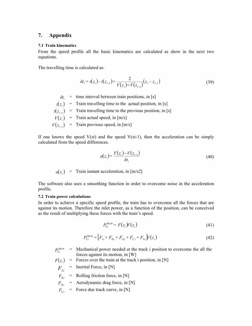
From the speed profile all the basic kinematics are calculated as show in the next two equations. The travelling time is calculated as:

( ) ( )( ) ( )

( )11

1

2−

−− −− ii

ii

iii zzzV+zV

=ztzt=δt (39)

iδt = time interval between train positions, in [s]

( )izt = Train travelling time to the actual position, in [s]

( )1−izt = Train travelling time to the previous position, in [s]

( )izV = Train actual speed, in [m/s]

( )1−izV = Train previous speed, in [m/s]

If one knows the speed V(zi) and the speed V(zi-1), then the acceleration can be simply calculated from the speed differences.

( ) ( ) ( )i

iii

δt

zVzV=za 1−−

(40)

( )iza = Train instant acceleration, in [m/s2]

The software also uses a smoothing function in order to overcome noise in the acceleration profile.

7.2 Train power calculations

In order to achieve a specific speed profile, the train has to overcome all the forces that are against its motion. Therefore the inlet power, as a function of the position, can be conceived as the result of multiplying these forces with the train’s speed.

( ) ( )ii

Mech

iT, zVzF=P (41)

[ ] ( )iiS,iC,iD,iR,iI,

Mech

iT, zVF+F+F+F+F=P (42)

Mech

iT,P = Mechanical power needed at the track i position to overcome the all the forces against its motion, in [W]

( )izF = Forces over the train at the track i position, in [N]

iI,F = Inertial Force, in [N]

iR,F = Rolling friction force, in [N]

iD,F = Aerodynamic drag force, in [N]

iC,F = Force due track curve, in [N]

iS,F = Force due track slope, in [N]

( )izV = Train speed at the track i position , in [m/s]

The force needed to accelerate the train can be broken down into the following components:

7.3 Inertial forces

To move forward, the train must provide enough energy to overcome the train’s inertia, which is directly related to its weight.

( ) ( )iITiI, zaM+M=F (43)

TM = Train total weight, in [kg]

IM = Train inertial mass, in [kg]

7.4 Rolling friction force

It is conceived, as force necessarily to move the wheels forward and is directly proportional to the weight of the load supported by the wheels. The magnitude of the friction force: Davis formula term for Rolling Friction:

( )( )i

'

TiR, zVB+AM=F ⋅ (44)

'

TM = Train total weight, in [ton]

A = Davis formula A empirical parameter for the train. B = Davis formula B empirical parameter for the train.

7.5 Aerodynamic drag

The force exerted on a train moving inside a tunnel, depends in a complex way upon the velocity of the train relative to the air, the viscosity and density of air, the shape of the train, the roughness of its surface and the tunnel cross-sectional area.

( )2iiD, zVDC=F ⋅⋅ (45)

C = Davis formula C empirical parameter for the tunnel. D = Davis formula D empirical parameter for the train.

For small values of the Reynolds number (called laminar flow since the flow is non-turbulent) the drag coefficient is inversely proportional to the velocity. This means that the drag force is only proportional to the train velocity. When the flow is turbulent the Reynolds number is large, and the drag coefficient D is approximately constant. This is the quadratic model of fluid resistance, in that the drag force is dependent on the square of the velocity.

7.6 Force due to track curve

This force is a result of the change in the accelerating vector.

r

EgM=F TC ⋅ (46)

E = Davis formula E empirical parameter for the train. g = Gravity acceleration, in [m/s2] r = Track segment curve radius, in [m]

7.7 Force due to track slope

Not always this force plays against motion. It depends on the direction in which the train is moving, down or up stream.

dl

dhgM=F TS

(47)

dh = track height difference with equal slope and curve radius, in dl = track length with equal slope and curve radius, in

7.8 Air flow model

Modelling the air flow inside the tunnel is quite a difficult problem. It has to take into account the air extractor system, the train’s piston effect, the chimney effect due to different air densities between the tunnel and ambient air, and also the different station relative height. Moreover, pressure differences are generated by stations passageways and ventilation shafts designs. For a more precise model, the fluid dynamic problem has to be taken into account, which is beyond from the scope of this work. A simplified model has been developed, which use mean air flow values and directions during each operational period.

7.9 Air flow calculations

atural Convection Air Flow:

In the non operational periods or so called “out service”, a natural convective air flow work as a heat carrier.

CSAV=v 4

air

4

air ⋅~

& (48)

4

airv& = Natural convection air flow, in [m3/s]

4

airV~

= Natural convection mean air speed, in [m/s]

CSA = Line segment cross section area, in [m2]

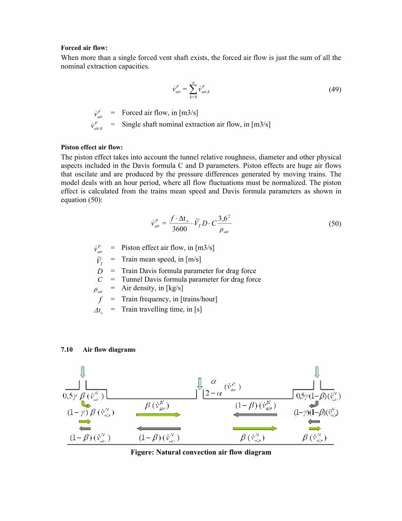
Forced air flow:

When more than a single forced vent shaft exists, the forced air flow is just the sum of all the nominal extraction capacities.

∑n

=k

F

kair,

F

air v=v0

&& (49)

F

airv& = Forced air flow, in [m3/s] F

kair,v& = Single shaft nominal extraction air flow, in [m3/s]

Piston effect air flow:

The piston effect takes into account the tunnel relative roughness, diameter and other physical aspects included in the Davis formula C and D parameters. Piston effects are huge air flows that oscilate and are produced by the pressure differences generated by moving trains. The model deals with an hour period, where all flow fluctuations must be normalized. The piston effect is calculated from the trains mean speed and Davis formula parameters as shown in equation (50):

air

T

P

airρ

CDVf

=v2

v 3,6~

3600

t⋅⋅

∆⋅& (50)

P

airv& = Piston effect air flow, in [m3/s]

TV~

= Train mean speed, in [m/s]

D = Train Davis formula parameter for drag force C = Tunnel Davis formula parameter for drag force

airρ = Air density, in [kg/s]

f = Train frequency, in [trains/hour]

v∆t = Train travelling time, in [s]

7.10 Air flow diagrams

Figure: atural convection air flow diagram

Figure: Forced air flow diagram

Figure: Piston effect air flow diagram

Figure: Tunnel air flow model diagram

7.11 HVAC model

The HVAC power consumption, as well as the heat rejected by the car to the tunnel, is a function of the amount of people on the car, the car inner comfort temperature, ambient conditions and the car technology. The influence of relative humidity is also considered.

7.12 Model inputs

Outside conditions:

Ambient temperature, outT

Ambient relative humidity, RH

Inside conditions:

Mean tunnel air temperature, tunnelT~

Figure: Forced air flow diagram

Figure: Piston effect air flow diagram

Figure: Tunnel air flow model diagram

The HVAC power consumption, as well as the heat rejected by the car to the tunnel, is a of the amount of people on the car, the car inner comfort temperature, ambient

conditions and the car technology. The influence of relative humidity is also considered.

[ºC]

outRH [%]

tunnel [ºC]

The HVAC power consumption, as well as the heat rejected by the car to the tunnel, is a of the amount of people on the car, the car inner comfort temperature, ambient

conditions and the car technology. The influence of relative humidity is also considered.

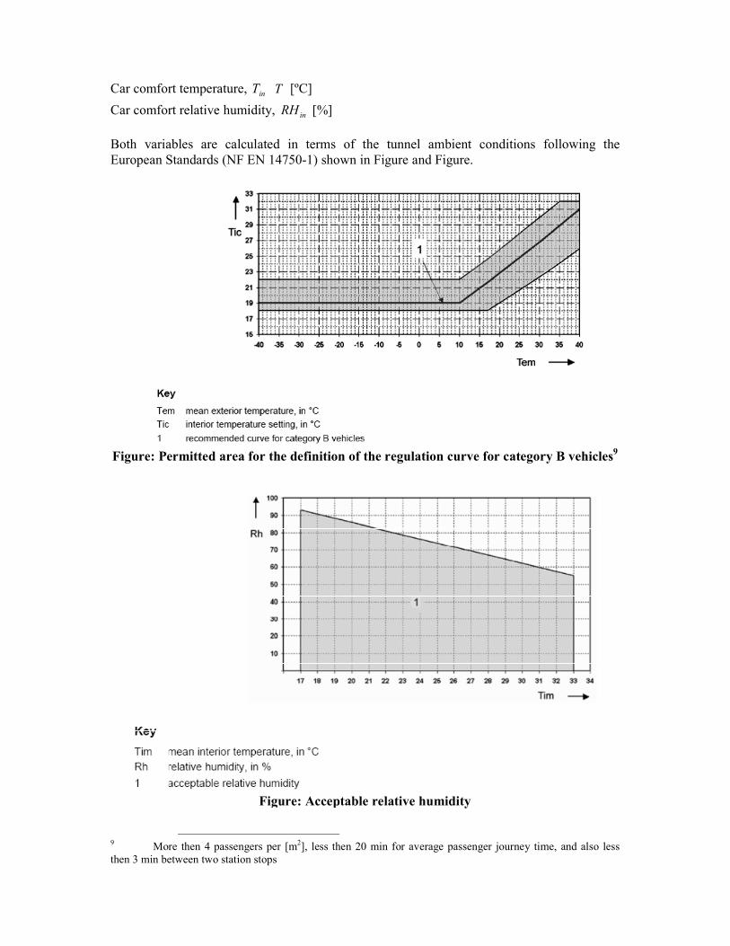
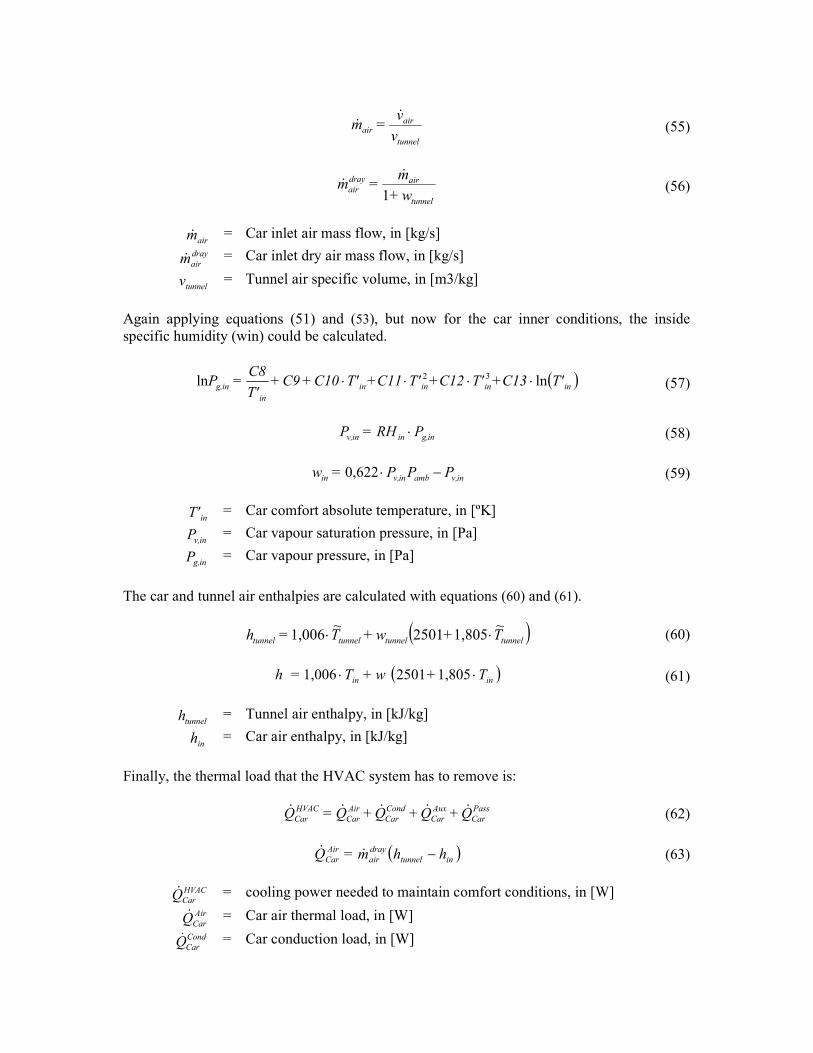
Car comfort temperature, inT T

Car comfort relative humidity, RH

Both variables are calculated in terms of the tunnel ambient conditions following the European Standards (NF EN 14750

Figure: Permitted area for the definition of the regulation curve for category B vehicles

Figure: Acceptable

9 More then 4 passengers per [mthen 3 min between two station stops

[ºC]

inRH [%]

Both variables are calculated in terms of the tunnel ambient conditions following the European Standards (NF EN 14750-1) shown in Figure and Figure.

itted area for the definition of the regulation curve for category B vehicles

Figure: Acceptable relative humidity

More then 4 passengers per [m2], less then 20 min for average passenger journey time, and also less

Both variables are calculated in terms of the tunnel ambient conditions following the

itted area for the definition of the regulation curve for category B vehicles

9

less then 20 min for average passenger journey time, and also less

Other Parameters Car air renovation, airv& [m3/s]

Heat exchange with the outside, trough the car’s surface, Cond

CarQ& [kW]

Car auxiliary power without HVAC system, Aux

CarQ& [ºkW]

Car passenger Sensible and Latent Heat, Pass

CarQ& [kW]

HVAC coefficient of performance, COP

7.13 Methodology

The car inlet air comes with a specific humidity and temperature which are calculated from the ambient conditions. The model neglects the station influences over the relative humidity. To get the ambient specific humidity ( ) ( )[ ]( )

airvapourout kgkgw / we use the following set of

equations:

( ) ( )outoutoutout

out

outg, T'+C13T'+C12T'+C11T'C10+C9+T'

C8=P lnln 32 ⋅⋅⋅⋅ (51)

outg,outoutv, PRH=P ⋅ (52)

outv,amb

outv,

tunneloutPP

P=w=w

−

⋅0,622 (53)

outT' = Ambient absolute temperature, in [ºK]

outv,P = Ambient vapor saturation pressure, in [Pa]

outg,P = Ambient vapor pressure, [Pa]

ambP = Ambient pressure, in [Pa]

Equation (51) coefficients are in Table: Coefficients for the vapor pressure equation shown:

Table: Coefficients for the vapor pressure equation

C8 -5800,2206 C9 1,3914993

C10 -0,04864024 C11 4,1765E-05 C12 -1,4452E-08 C13 6,5459673

The car inlet air mass flow depends on the tunnels air specific volume and it’s calculated as presented in equations (54), (55) and (56):

( ) ( )310

1,60781273~

0,2871

⋅⋅⋅⋅

amb

tunneltunneltunnel

P

w++T=v (54)

tunnel

airair

v

v=m

&& (55)

tunnel

airdray

airw+

m=m

1

&& (56)

airm& = Car inlet air mass flow, in [kg/s] dray

airm& = Car inlet dry air mass flow, in [kg/s]

tunnelv = Tunnel air specific volume, in [m3/kg]

Again applying equations (51) and (53), but now for the car inner conditions, the inside specific humidity (win) could be calculated.

( )inininin

in

ing, T'+C13T'+C12T'+C11T'C10+C9+T'

C8=P lnln 32 ⋅⋅⋅⋅ (57)

ing,ininv, PRH=P ⋅ (58)

(59)

inT' = Car comfort absolute temperature, in [ºK]

inv,P = Car vapour saturation pressure, in [Pa]

ing,P = Car vapour pressure, in [Pa]

The car and tunnel air enthalpies are calculated with equations (60) and (61).

( )tunneltunneltunneltunnel T+w+T=h~

1,8052501~

1,006 ⋅⋅ (60)

( )inin T+w+T=h ⋅⋅ 1,80525011,006 (61)

tunnelh = Tunnel air enthalpy, in [kJ/kg]

inh = Car air enthalpy, in [kJ/kg]

Finally, the thermal load that the HVAC system has to remove is:

Pass

Car

Aux

Car

Cond

Car

Air

Car

HVAC

Car Q+Q+Q+Q=Q &&&&& (62)

( )intunnel

dray

air

Air

Car hhm=Q −&& (63)

HVAC

CarQ& = cooling power needed to maintain comfort conditions, in [W] Air

CarQ& = Car air thermal load, in [W] Cond

CarQ& = Car conduction load, in [W]

inv,ambinv,in PPP=w −⋅0,622

Aux

CarQ& = Car auxiliary power, in [W] Pass

CarQ& = Car passenger sensible and latent heat flow, in [W]

7.14 Simulation procedures and assumptions

• To perform the simulations, the system (the subway line) is divided in discrete segments ∆z of length 1 [m], where the speed and the air temperature are assumed constant. In what concerns the calculation core, the model evaluates separately each track segment applying to it the energy balance model described previously.

• There are two main systems that the software evaluates: “The Single Train System” and “The Line System”. The first system, measures the performance of a single train running in a specific way. As each travelling way has its own speed profile, they are treated at each iteration separately. Also we recognize two travelling ways: LR (from left to right) and RL (from right to left). The second system evaluated, is in charge of the line energy balance and thus, temperature predictions.

• A train running in a specific way generates a Heat Profile over the track. This Heat profile is added with the heat rejected in each station in order to generate a unique heat profile a cross the whole line, for a specific time interval.

• Each track section (the tunnel that interconnect two stations) is isolated from the rest of the tunnels, in the sense that stations work as boundary conditions at the beginning of each iteration for temperature predictions, and this generic situation is extended to the general system.

• As stations also have specific properties (length, surface area, auxiliary power, people coming in and out, etc.) and, moreover, they are affected by the track sections that are in both sides of it, a line will be considered as a non-homogeneous tunnel. This means that stations will linked the track sections in order to create a unique tunnel, but with different geometrical properties. The non homogeneous tunnel has been conceived as a semi infinite solid with variable surface temperature, as boundary condition. The ground that surrounds the tunnel acts as a sink and can store energy from ambient conditions along the year, keeping ground temperature almost constant depending on the season.

• Two separately air flows are defined: From Left to Right and From Right to Left. • The air flow sources are: Forced, Natural and Piston effect induce air flows. • Fresh air comes through the stations and flows through the tunnels, but, also air from

the previous section leaks into the Station. As the air flow rate must keep constant (not mass gaining are allowed), an arbitrary parameter (γ ) is introduce to measure how much new air came to the station and how much air came from the previous section. An (γ ) equal to 1, means that all the air comes from the outside.

• A chimney effect parameter ( β ) is defined, which measures the influence of one

station over the other. If ( β ) equals to 1, it means that the natural forced air flows only from station A to station B.