
JONI TURUNEN - CERN · CERN-THESIS-2011-174 //2011 JONI TURUNEN Parametric study of the cost...
84
CERN-THESIS-2011-174 //2011 JONI TURUNEN Parametric study of the cost estimate for ultra precision RF components Master of Science Thesis Prof. Saku Mäkinen has been appointed as the examiner at the Council Meeting of the Faculty of Business and Technology Management on October 5th, 2011.
Transcript of JONI TURUNEN - CERN · CERN-THESIS-2011-174 //2011 JONI TURUNEN Parametric study of the cost...
CER
N-T
HES
IS-2
011-
174
//20
11
JONI TURUNEN
Parametric study of the cost estimate for ultra precision RF components
Master of Science Thesis
Prof. Saku Mäkinen has been appointed as the examiner at
the Council Meeting of the Faculty of Business and
Technology Management on October 5th, 2011.
i
ABSTRACT
TAMPERE UNIVERSITY OF TECHNOLOGY
Master’s Degree Programme in Industrial Engineering and Management
TURUNEN, JONI: Parametric study of the cost estimate for ultra precision RF
components
Master of Science Thesis, 68 pages, 4 appendices (4 pages)
December 2011
Major: Industrial Management
Examiner: Professor Saku Mäkinen
Keywords: Ultra precision machining, shape accuracy, surface roughness, cost estimate,
diamond machining, OFE copper
The purpose of this thesis was to find out how the shape accuracy and surface roughness
of an RF disk affect the machining time of a disk and the cost of the accelerating
structures. The disks in question are part of a future Compact Linear Collider (CLIC)
project. This thesis was made because the price of a single disk is a major cost driver of
the CLIC project. The cost of a disk is composed mainly of the time consuming ultra
precise machining with expensive diamond tools. The surface roughness Ra 25 nm and
shape accuracy 5 µm requirements are the reason for the need of ultra precision. The
total number of disks to be produced for CLIC at 3 TeV center-of-mass energy is
roughly 4.1 million, thus the project is a typical example of mass production where
learning curves can be applied.
Based on the theoretical calculations, changing the surface roughness Ra from 25 nm to
100 nm decreases the total ultra precise machining from 644 minutes to 311 minutes
with current tooling and machining parameters. The effect of shape accuracy to the cost
proved to be hard to estimate. Going from shape accuracy 5 µm to 20 µm will cause
cost savings in tooling and machinery. However, because the connection between shape
accuracy and surface roughness is not exactly known at micro- and nanometre scale and
the wear of the replacement for a single crystal controlled waviness diamond tool is not
exactly known in series production, the cost effect of shape accuracy relaxation could
not be estimated. Changing the ultra precise machines to cheaper precise machines will
only have a marginal effect on the cost of the accelerating structure.
In conclusion, it can be said that after applying the learning curves, the ultra precise
machining times drop to a level at which the project is viable. Regardless of the learning
percent used, the change of surface roughness Ra from 25 nm 100 nm cuts the ultra
precise machining time roughly to half. This means that the total cost of the accelerating
structures reduces 6–16 percent depending on the number of production lines and the
applied learning percentages, which will probably be in the order of 90 to 95 percent.
To verify the results of this thesis, machining tests with similar tools and machining
parameters should be done.
ii
TIIVISTELMÄ
TAMPEREEN TEKNILLINEN YLIOPISTO
Tuotantotalouden koulutusohjelma
TURUNEN, JONI: Parametrinen tutkimus suurta koneistustarkkuutta vaativien RF
komponenttien kustannusarviosta
Diplomityö, 68 sivua, 4 liitettä (4 sivua)
Joulukuu 2011
Pääaine: Teollisuustalous
Tarkastaja: professori Saku Mäkinen
Avainsanat: Muototarkkuus, pinnankarheus, kustannusarvio, timanttityöstö, OFE kupari
Tämän työn tarkoituksena oli selvittää miten RF-kiekon pinnankarheus ja
muototarkkuus vaikuttavat valmistettavan kiekon koneistusaikaan ja
kiihdytinrakenteiden kustannuksiin. Tutkitut kiekot ovat osa tulevaa Compact Linear
Collider (CLIC) projektia. Tutkimus suoritettiin, koska yksittäisen kiekon hinta on
merkittävä kustannustekijä koko projektissa. Kiekkojen kustannukset muodostuvat
pääasiassa aikaa vievästä timanttityöstöstä ja kalliista timanttityökaluista. Kiekkoille
asetetut pinnankarheus Ra 25 nm ja muototarkkuus 5 µm vaatimukset ovat syynä
timanttityöstön tarpeeseen. Kun pidetään mielessä, että CLIC suunnitellulla 3 TeV
energialla tarvitsee noin 4.1 miljoonaa kiekkoa, voidaan puhua massatuotannon
tyyppiesimerkistä, johon voidaan soveltaa oppimiskäyriä.
Suoritettujen teoreettisten laskelmien perusteella havaittiin, että pienentämällä kiekon
pinnankarheusvaatimusta Ra 25 nanometristä 100 nanometriin, kiekon timanttityöstöön
käytetty kokonaiskoneistusaika putoaa 644 minuutista 311 minuuttiin tällä hetkellä
käytetyillä työkaluilla ja koneistusparametreilla. Muototarkkuusvaatimuksen
pienentäminen 5 mikrometristä 20 mikrometriin aiheuttaa säästöjä sekä kone- että
työkalukustannuksissa. Korvaamalla yksikiteiset muotokontrolloidut timanttityökalut
halvemmilla työkaluilla, saavutettaisiin kustannussäästöjä. Koska korvaavien työkalujen
kulumista tarkkuustyöstössä ei tunneta, ei kustannusvaikutusta pystytty arvioimaan.
Ultratarkkuusluokan jyrsintä- ja sorvauskoneiden vaihto halvempiin ei aiheuta
merkittäviä kustannussäästöjä
Yhteenvetona voidaan todeta, että oppimiskäyrien soveltamisen jälkeen kiekkojen
timanttityöstöajat putoavat tasolle, jolla projektin toteuttaminen on mahdollista.
Riippumatta käytetyistä oppimiskertoimista pinnankarheusvaatimuksen pudottaminen
Ra 25 nanometristä 100 nanometriin pudottaa käytetyn timanttityöstöajan noin puoleen.
Tämä tarkoittaa kiihdytinrakenteiden kokonaisvalmistuskustannusten alenemista 6–16
prosentilla riippuen tuotantolinjojen määrästä ja käytetystä oppimiskertoimesta, joka
asettunee välille 90–95 prosenttia. Tämän työn tulosten vahvistamiseksi tulisi suorittaa
koneistustestejä käyttäen vastaavia työkaluja ja koneistusparametreja.
iii
PREFACE
This thesis has been a long process during which there has been setbacks and
difficulties. However, all of them have been overcome and the project has successfully
come to an end. Working at CERN has been an experience that I will never forget. For
this I am grateful for CERN and Helsinki Institute of Physics for providing me an
opportunity to work and do my thesis at CERN. The one and half years I have spent at
CERN have taught me a lot. The international environment and working with the
cutting edge technologies have been eye-opening and inspiring.
I would like thank my supervisors Kenneth Österberg at Helsinki Institute of Physics
and Germana Riddone at CERN as well as my examiner Saku Mäkinen at Tampere
University of Technology for the valuable guidance and comments. In addition, I would
like thank all the members of CLIC team, who helped me with this thesis. Especially, I
would like to thank Said Atieh for helping me in the technical part of the machining. I
am also grateful to Tero Halme for the mathematical consultation that he provided in his
spare time. Last but not least I like would like express my deepest gratitude to my
friends and family who have supported me during the thesis process.
Geneva, Switzerland. 18th of November 2011.
Joni Turunen
iv
TABLE OF CONTENTS
ABSTRACT ......................................................................................... i
TIIVISTELMÄ ..................................................................................... ii
PREFACE .......................................................................................... iii
TABLE OF CONTENTS .................................................................... iv
NOTATION ........................................................................................ vi
ABBREVIATIONS ............................................................................ vii
LIST OF FIGURES .......................................................................... viii
LIST OF TABLES .............................................................................. x
1. INTRODUCTION .......................................................................... 1
1.1. Background .......................................................................................... 1
1.2. Research problem, objectives and limitations ....................................... 2
1.3. Research methodology and the structure of the thesis ......................... 3
2. RESEARCH ENVIRONMENT ..................................................... 4
2.1. CERN ................................................................................................... 4
2.2. CLIC Study ........................................................................................... 5
2.2.1. CLIC two-beam acceleration and two-beam module ................ 7
2.2.2. CLIC accelerating structures .................................................... 8
2.2.3. CLIC disks .............................................................................. 10
2.2.4. Error sources in accelerating structures ................................. 12
3. MANUFACTURING AN ACCELERATING STRUCTURE AND
A DISK .............................................................................................. 14
3.1. Manufacturing an accelerating structure ............................................. 14
3.2. Manufacturing a disk ........................................................................... 15
3.2.1. Material ................................................................................... 16
3.2.2. Machining techniques ............................................................. 17
3.2.3. Need of ultra precision machining .......................................... 18
3.2.4. Heat treatments ...................................................................... 28
3.2.5. Main challenges in machining a disk ...................................... 28
4. GEOMETRICAL MEASUREMENTS ......................................... 30
4.1. Measurement techniques ................................................................... 30
4.1.1. Contact measurement ............................................................ 30
4.1.2. Non-contact measurement ..................................................... 31
4.2. Measured parameters ......................................................................... 32
4.2.1. Surface roughness ................................................................. 32
v
4.2.2. Shape accuracy ...................................................................... 35
4.2.3. Flatness .................................................................................. 35
4.3. Metrology at factory and at CERN ...................................................... 36
5. THEORETICAL MODEL FOR MACHINING OF DISKS ........... 38
5.1. Introduction to machining models ....................................................... 40
5.2. Theoretical machining parameters...................................................... 40
5.2.1. Milling ..................................................................................... 40
5.2.2. Turning ................................................................................... 41
5.3. Theoretical machining times ............................................................... 42
5.3.1. Milling ..................................................................................... 42
5.3.2. Turning ................................................................................... 43
5.4. Theoretical machining times for a test disk ......................................... 44
5.4.1. Milling ..................................................................................... 44
5.4.2. Turning ................................................................................... 46
5.4.3. Overall times........................................................................... 48
5.5. Error considerations ............................................................................ 48
6. COST ESTIMATE METHOD AND PARAMETERS .................. 50
6.1. Cost method ....................................................................................... 50
6.2. Learning curves .................................................................................. 50
6.3. Evaluated parameters ......................................................................... 53
6.3.1. Surface roughness ................................................................. 53
6.3.2. Shape accuracy ...................................................................... 54
6.4. Parametric cost estimate .................................................................... 55
7. DISCUSSION ............................................................................. 57
8. CONCLUSIONS ......................................................................... 60
BIBLIOGRAPHY .............................................................................. 62
APPENDICES (4 pieces)................................................................. 68
vi
NOTATION
a Learning percentage
A Area
Ae Radial depth of cut (In milling)
Ap Axial depth of cut
c(1) In general, a cost of a prototype; in this thesis, a time to
produce a prototype
C(n) Cumulative cost of n units
ϵx Horizontal emittance
ϵy Vertical emittance
hc Minimum chip thickness
f Tool feed (In turning, comparable to Ae)
l Flat top of a toroidal cutting tool
L Length
n The number of units to be produced per production line
r Radius of cutting tool
R Tooltip radius
Ra Arithmetic average of surface roughness (ISO-4287)
Rz Maximum height of profile (ISO-4287)
V Spindle speed (rpm)
Vf Feed rate
z(x) Surface profile height (ISO-4287)

vii
ABBREVIATIONS
AS Accelerating Structure
CERN European Organization for Nuclear Research
CLIC Compact LInear Collider
CDR Conceptual Design Report
CMM Coordinate measuring machine
CMF Choke mode flange
CTF CLIC test facility
CVD Chemical vapour deposition
DB Drive beam
eV Electronvolt
HOM High-order mode
HSS High speed steel
ILC International Linear Collider
LEP Large Electron-Positron collider
LHC Large Hadron Collider
Linac Linear particle accelerator
MB Main beam
OFE Oxygen-free electrolytic (In context of copper)
PCD Polycrystalline diamond
PETS Power extraction and transfer structure
RF Radio frequency
SEM Scanning electron microscope
SPDT Singe point diamond turning
UNS The Unified Numbering System
WFM Wakefield monitor
viii
LIST OF FIGURES
Figure 1.1. CLIC accelerating structure prototype (Picture courtesy of CERN). ............ 1
Figure 1.2. A disk under microscope for inspection (Picture courtesy of CERN). .......... 2
Figure 2.1. Current project plan for CLIC (Stapnes 2011). ............................................ 5
Figure 2.2. Overall layout of CLIC at 3 TeV. ................................................................ 6
Figure 2.3. The CLIC two-beam scheme, with the main beam accelerated by energy
provided from the lower-energy, high-current drive beam (Braun et al. 2008b). . 7
Figure 2.4. Two-beam module (Model by A. Samoshkin, courtesy of CERN). .............. 8
Figure 2.5. Accelerating structure - TD24 R0.5 (Model by A. Solodko, courtesy of
CERN). ............................................................................................................. 9
Figure 2.6. Accelerating structure - TD26 CC SiC (Model by A. Solodko, courtesy of
CERN). ........................................................................................................... 10
Figure 2.7. TD24 R0.5 disk drawing (Drawing by A. Solodko, courtesy of CERN). .... 11
Figure 2.8. TD26 CC SiC disk drawing (Drawing by A. Solodko, courtesy of CERN). 12
Figure 2.9. “Bookshelfing” phenomena i.e. a systematic tilt of the disks (Zennaro
2008a). ............................................................................................................ 13
Figure 2.10. The misalignment of the iris aperture with respect to the axis of the cell and
damping waveguides (Samoshkin 2011). ......................................................... 13
Figure 3.1. Manufacturing procedure for a TD24 R0.5 AS (Solodko et al. 2010). ........ 14
Figure 3.2. A typical flow for machining of a disk (Machining flow by S. Atieh). ....... 16
Figure 3.3. Milling (CustomPartNet 2007). ................................................................. 17
Figure 3.4. Turning (CustomPartNet 2007). ................................................................ 18
Figure 3.5. Different machining precisions (S. Atieh). ................................................. 19
Figure 3.6. Taniguchi equivalent for cutting processes updated by Corbett et al. and
Byrne et al. (Taniguchi 1983; Corbett et al. 2000; Byrne et al. 2003). .............. 20
Figure 3.7. Iris area of a disk with both ultra precise turning and milling visible (Picture
by A. Olyunin, courtesy of CERN). ................................................................. 21
Figure 3.8. Backside of a turned disk (Picture by D. Glaude, courtesy of CERN). ....... 22
Figure 3.9. Surfaces machined by a diamond tool on the left and by a WC tool on the
right (SEM micrographs by G. Arnau, courtesy of CERN). .............................. 24
Figure 3.10. WC (left) and PCD (right) tools after 9-10 minutes of turning ultra-fine
grained OFE copper (Morehead et al. 2007)..................................................... 24
Figure 3.11. An SEM micrograph of a diamond end mill (Yan et al. 2010). ................ 25
Figure 3.12. A) A diamond tool with controlled waviness. B) A diamond tool with non-
controlled waviness. (Vavrille 2003) ............................................................... 26
Figure 3.13. On the left single crystal diamond controlled waviness tool, on the right
CVD ball end mill (Technodiamant 2011). ...................................................... 27
ix
Figure 3.14. SEM micrograph of a copper disk with both milling and turning marks
visible (Micrograph by M. Aicheler, courtesy of CERN). ................................ 29
Figure 4.1. A basic contact measurement system (Grzesik 2008). ................................ 31
Figure 4.2. Variance of scattering angle on different surface roughnesses. a) Very
smooth surface; variance very small. b) Very rough surface; variance very large.
c) Intermediate surface; variance of intermediate value. (Jolic et al. 1994) ....... 31
Figure 4.3. A 2D surface profile represents the combined effects of roughness, waviness
and form (Adapted from Grzesik 2008). .......................................................... 33
Figure 4.4. Surface roughness measurement (Measurement by D. Glaude, courtesy of
CERN). ........................................................................................................... 34
Figure 4.5. Shape accuracy measurement (magnified 100 times). The solid line is the
target profile, the two dotted lines are the tolerances (± 2.5 µm) and the solid line
with dots is the measurement (Measurement by VDL Enabling Technologies
Group). ............................................................................................................ 35
Figure 4.6. Flatness measurement (Measurement by D. Glaude). ................................ 36
Figure 5.1. Plane surface approximated by spherical cuts. ........................................... 38
Figure 5.2. Circular motion approximated by linear motion in x-y-plane (Adapted from
Yoshioka & Shinno 2011). .............................................................................. 39
Figure 5.3. Factors affecting surface roughness (Benardos & Vosniakos 2003). .......... 40
Figure 5.4. An ideal surface profile generated by a toroidal end mill. .......................... 42
Figure 5.5. An ideal surface profile generated by turning with a round tooltip tool. ..... 43
Figure 5.6. Theoretical finishing milling times for a toroidal end mill with different
corner radiuses (r). The flat part of the tool is 0.10 mm, the offset is 0.05 mm
and the inclination angle is 0°. ......................................................................... 45
Figure 5.7. Iris area of a disk showing different amounts of passes in turning (Picture
courtesy of CERN). ......................................................................................... 46
Figure 5.8. Theoretical time used for ultra precision turning of TD24R0.5 with different
feed rates. Crosses mark the 4 and 6 mm/min feed rates................................... 46
Figure 6.1. Learning curves with three different learning percent. ............................... 52
Figure 6.2. Learning curves with three different learning percent and saturation at 100
units. ............................................................................................................... 52
Figure 8.1. Micromachining relative to other machining processes (Byrne et al. 2003).
........................................................................................................................ 61
x
LIST OF TABLES
Table 3.1. Typical machine requirements. ................................................................... 23
Table 3.2. Typical requirements for tools. ................................................................... 27
Table 4.1. Surface profile parameter definitions (ISO-4287). ...................................... 34
Table 5.1. Typical process parameters for ultra precision milling of OFE-copper with a
diamond tool (Reinecke & Müller 2008). ......................................................... 41
Table 5.2. Typical process parameters for ultra precision turning of OFE-copper with a
diamond tool (Reinecke & Müller 2008). ......................................................... 41
Table 5.3. Typical process parameters for ultra precision turning of OFE-copper with a
diamond tool (Hwang et al. 2008). ................................................................... 41
Table 5.4. Typical feed rates (mm/min) of toroidal end mill with different corner
radiuses. .......................................................................................................... 44
Table 5.5. Theoretical values for single point diamond turning. ................................... 47
Table 5.6. Total ultra precision machining times for a prototype disk. ......................... 48
Table 6.1. Learning percentages of selected reference industries (Fessia et al. 2007). .. 51
Table 6.2. Production per the number of production lines. ........................................... 53
Table 6.3. Average ultra precision machining times after implementing learning curves,
times in minutes. ............................................................................................. 53
Table 6.4. Average ultra precision machining times after implementing learning curves
and saturation after 20000 units are produced, times in minutes. ...................... 54
Table 6.5. The absolute change in ultra precision machining time in minutes for the
change of surface roughness Ra from 25 to 100 nm. ........................................ 54
Table 6.6. The increase of the average ultra precision machining time due to applying
saturation of learning after 20000 units are produced. ...................................... 54
Table 6.7. Relative cost of manufacturing the AS for a 3 TeV CLIC with different
surface roughnesses, in two, three or four separate production lines and with
85%, 90% and 95% learning percent................................................................ 55
Table 6.8. Relative cost of manufacturing the AS for a 3 TeV CLIC with different
surface roughnesses, in two, three or four separate production lines and with
85%, 90% and 95% learning percent and saturation after 20000 units are
produced.......................................................................................................... 55
Table 6.9. The effect of applying saturation on the learning to the total cost estimate for
the AS for a 3 TeV CLIC. ................................................................................ 56
Table 7.1. The average machining times as a percentage of the prototype machining
time after applying learning curves. ................................................................. 57

xi
Table 7.2. The average machining times as a percentage of the prototype machining
time after applying saturation to learning curves after 20000 disks are produced.
........................................................................................................................ 57
Table 7.3. The total cost saving of reducing surface roughness Ra from 25 nm to 100
nm for the AS for a 3 TeV CLIC. .................................................................... 58
Table 7.4. The total cost saving of reducing surface roughness Ra from 25 nm to 100
nm for the AS for a 3 TeV CLIC when saturation of learning after 20000 units is
assumed. .......................................................................................................... 59
1
1. INTRODUCTION
1.1. Background
In 2009, a comprehensive industrialization study for the cost estimate of radio
frequency (RF) accelerating structures was started at CERN, European Organization for
Nuclear Research. The study was part of the Compact LInear Collider (CLIC) study,
which aims to build a nearly 50-kilometre linear collider. CLIC is planned to collide
electrons and positrons at a centre-of-mass energy that is currently designed to be up to
3 TeV. Currently the CLIC study is approaching the end of the conceptual design phase,
where the feasibility of CLIC has been demonstrated. The conceptual design report
(CDR) will contain a consistent set of parameters and a first idea of technical
implementation of the project. The detailed technical design will follow.
The RF Structure Development activity, in which the author is also a member, studies
the design and manufacturing of the RF structures. An industrialization study (Uusimäki
& Saifoulina 2010) ordered by the RF Structure production team is the base, which this
thesis relies on. In the study, three companies conducted each on their own an estimate
for the price for manufacturing RF components for the CLIC accelerating structures
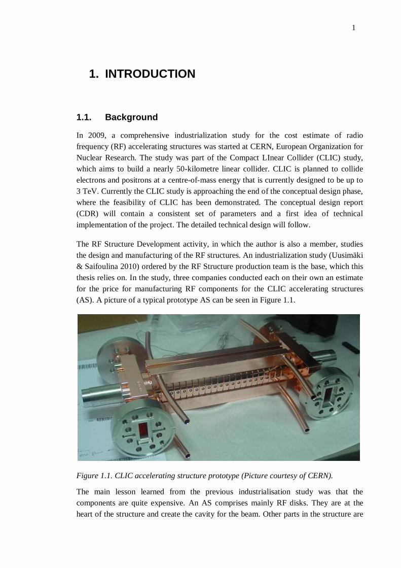
(AS). A picture of a typical prototype AS can be seen in Figure 1.1.
Figure 1.1. CLIC accelerating structure prototype (Picture courtesy of CERN).
The main lesson learned from the previous industrialisation study was that the
components are quite expensive. An AS comprises mainly RF disks. They are at the
heart of the structure and create the cavity for the beam. Other parts in the structure are
2
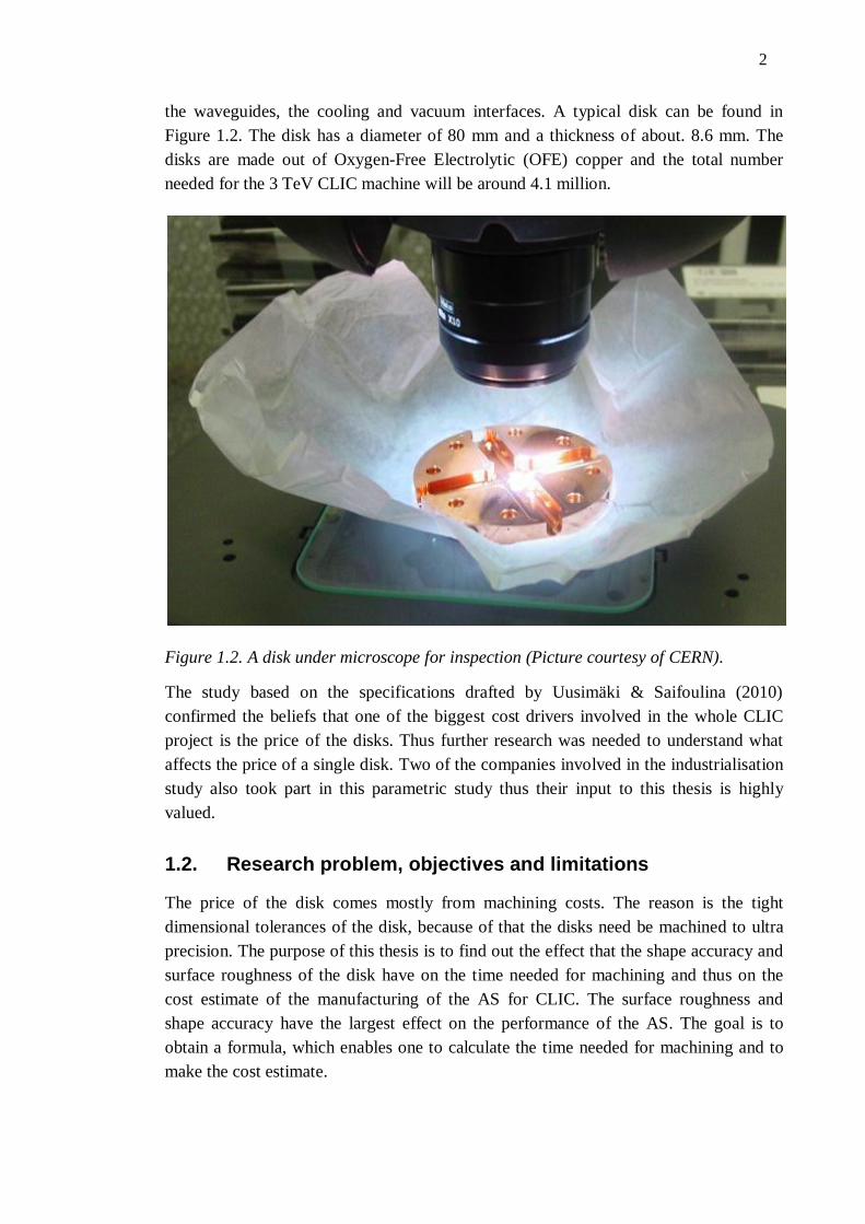
the waveguides, the cooling and vacuum interfaces. A typical disk can be found in
Figure 1.2. The disk has a diameter of 80 mm and a thickness of about. 8.6 mm. The
disks are made out of Oxygen-Free Electrolytic (OFE) copper and the total number
needed for the 3 TeV CLIC machine will be around 4.1 million.
Figure 1.2. A disk under microscope for inspection (Picture courtesy of CERN).
The study based on the specifications drafted by Uusimäki & Saifoulina (2010)
confirmed the beliefs that one of the biggest cost drivers involved in the whole CLIC
project is the price of the disks. Thus further research was needed to understand what
affects the price of a single disk. Two of the companies involved in the industrialisation
study also took part in this parametric study thus their input to this thesis is highly
valued.
1.2. Research problem, objectives and limitations
The price of the disk comes mostly from machining costs. The reason is the tight
dimensional tolerances of the disk, because of that the disks need be machined to ultra
precision. The purpose of this thesis is to find out the effect that the shape accuracy and
surface roughness of the disk have on the time needed for machining and thus on the
cost estimate of the manufacturing of the AS for CLIC. The surface roughness and
shape accuracy have the largest effect on the performance of the AS. The goal is to
obtain a formula, which enables one to calculate the time needed for machining and to
make the cost estimate.
3
The research question can be formulated as follows: How will the machining time and
thus the price change if we relax the initial tolerances of the disks?
The current requirements for the shape accuracy and surface roughness, 5 µm and Ra 25
nm respectively, are due to the requirements for beam dynamics and RF. A question has
been raised what would happen if the requirements would be relaxed. Would the time
needed for machining decrease dramatically? Would the cost estimate decrease
dramatically? Is the relationship linear or nonlinear? These questions will be studied in
this thesis.
The experience and knowledge learned from the machining of ultra precision
components can be used also in case the design of the disk changes as the shape and
tolerances will still be similar.
1.3. Research methodology and the structure of the thesis
This thesis covers theoretical study. Theoretical part includes the relevant theory of
machining and the special features of ultra precise machining. Because the required
dimensional tolerances are tight, a brief description of how to verify them is done in the
form of metrology. The calculated values are analysed and then parameterised and
finally a parameterised cost estimate is presented.
The machining process considered in this thesis is one of several that have been tested
and the resulting disks are known to meet the requirements. It is thus a validated method
for machining a disk meeting the specifications although certainly not the only one.
The structure of the thesis is as follows. The research environment at CERN and in
CLIC is introduced in chapter 2. The manufacturing flow and one part of it, machining
flow, are introduced in chapters 3 and 4. The quality control is presented in chapter 5 in
the form of metrology. The theoretical method for machining is introduced in chapter 6,
whereas chapter 7 describes the cost parameterisation method. The thesis will end with
discussion and conclusion.
4
2. RESEARCH ENVIRONMENT
This chapter introduces CERN and CLIC as a research environment. The role of the RF
structures in the accelerator is described and the operation principle of CLIC is showed
briefly. The term “ultra precision” will be used throughout this thesis (see chapter
3.2.3). A short explanation is that when talking about ultra precision the shape accuracy
of a piece is in the region of one µm or less.
2.1. CERN
CERN, European Organization for Nuclear Research, is one of the world’s largest
centres for scientific research. CERN is studying the structure of matter and how it
interacts. The research done at CERN includes fundamental physics. To learn about
these fundamentals and the constituents of the matter, the physicists try to create the
same conditions which were prevailing at the birth of the universe. These conditions can
be created by colliding particles. The main instruments used at CERN are particle
accelerators. Particles are accelerated to high energies and then let to collide with each
other. At the point of collision, a very precise detector records the collision and allows
physicists to study what has happened. (CERN 2011)
CERN will provide particle accelerators and infrastructure required for high-energy
physics experiments. Particularly, as the home of the world-wide web, CERN also has a
quite extensive computing centre and both the needed capacity to save all data from the
experiments and the network to transfer the data to physicists all around the world. At
the moment, CERN has 20 member states, who contribute to the capital and operation
costs of the programmes of CERN. Currently nearly 2400 people are employed by
CERN and every year CERN has around 10000 visiting scientists. CERN’s main
laboratory is located in Geneva near the border between Switzerland and France.
(CERN 2011)
The biggest ongoing project at CERN at the moment is the Large Hadron Collider
(LHC). The LHC is the world’s largest particle accelerator after Large Electron-Positron
Collider (LEP). As the LHC still remains to be the most complex machine ever being
built, there are already new projects going on at CERN which will one day take LHC’s
place as the most complex machine in the world. While LHC is still up and running
giving the long waited answers to the fundamentals of physics, the post-LHC era is
being planned. The new project aims to complete the results from the LHC. The new
project is called CLIC and it stands for Compact LInear Collider. The CLIC project
5
aims at building even bigger and more complex machine that complements the results
of the LHC. (CERN 2011)
2.2. CLIC Study
The CLIC is a study for a future electron-positron collider, which would be unique with
its capabilities of high energy (0.5-3 TeV), high luminosity (6 x 1034
cm-2
s-1
) and very
high precision (colliding beam bunches at a size of about 1 x 40 nm). CLIC would make
possible to explore a new energy region above the capabilities of existing particle
accelerators. It would provide fundamental physics information complementarily to the
LHC and lower-energy electron-positron colliders, as a result of its unique combination
of high energy and experimental precision. (Braun et al. 2008a)
The CLIC is currently a feasibility study to prove that the concepts will work in reality.
The next step for the study is at the end of 2011 when the conceptual design report for
CLIC will be ready. The conceptual design report (CDR) is supposed to cover
descriptions of the physics, the accelerator and the detectors, the site facilities, report on
research and development activities on critical issues, the results of feasibility studies,
cost issues and drivers as well as a proposal for the objectives and work plan for the
post-CDR phase. The project implementation would start at the earliest in 2017.
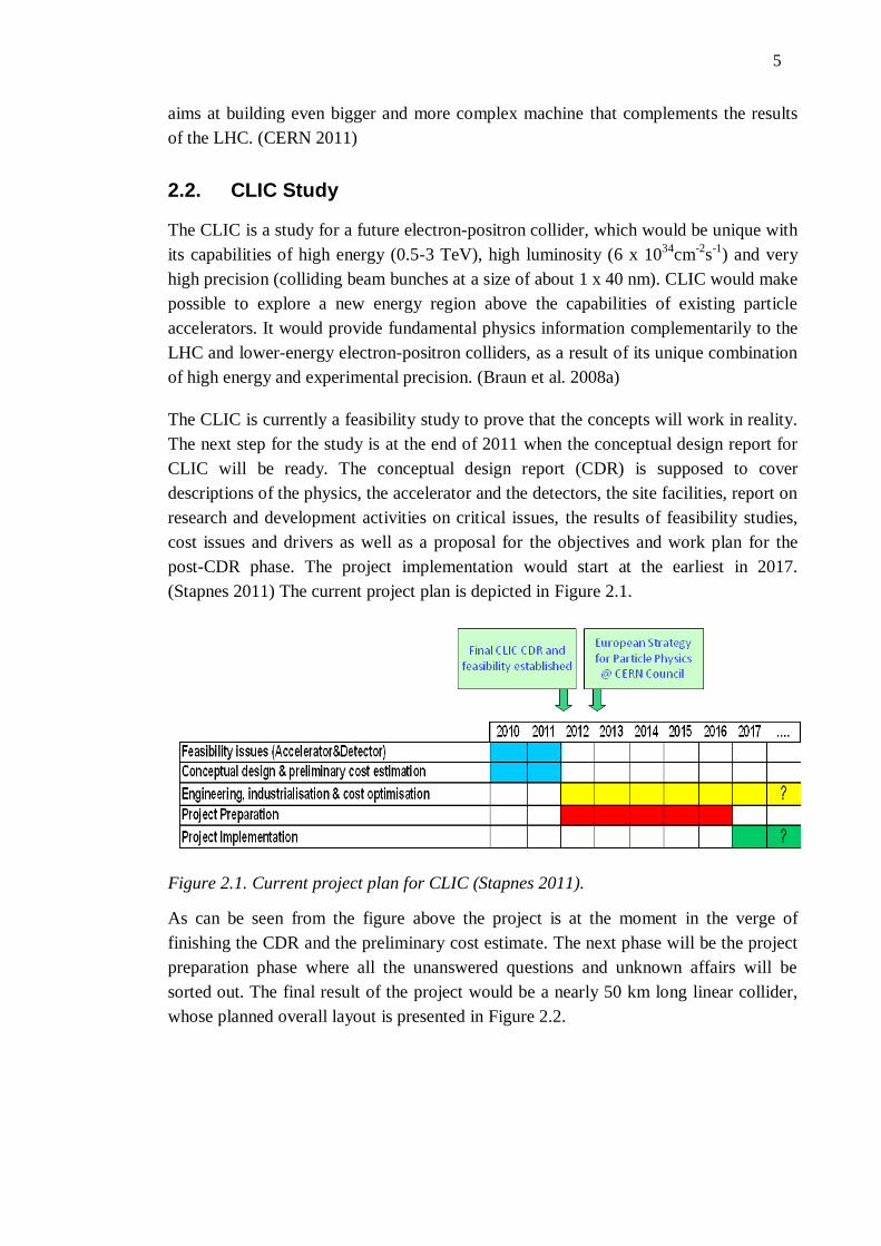
(Stapnes 2011) The current project plan is depicted in Figure 2.1.
Figure 2.1. Current project plan for CLIC (Stapnes 2011).
As can be seen from the figure above the project is at the moment in the verge of
finishing the CDR and the preliminary cost estimate. The next phase will be the project
preparation phase where all the unanswered questions and unknown affairs will be
sorted out. The final result of the project would be a nearly 50 km long linear collider,
whose planned overall layout is presented in Figure 2.2.
6
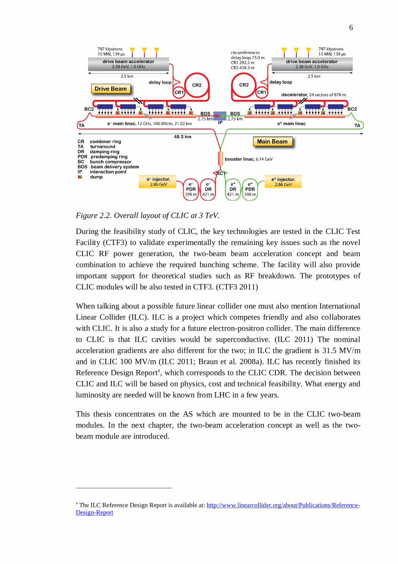
Figure 2.2. Overall layout of CLIC at 3 TeV.
During the feasibility study of CLIC, the key technologies are tested in the CLIC Test
Facility (CTF3) to validate experimentally the remaining key issues such as the novel
CLIC RF power generation, the two-beam beam acceleration concept and beam
combination to achieve the required bunching scheme. The facility will also provide
important support for theoretical studies such as RF breakdown. The prototypes of
CLIC modules will be also tested in CTF3. (CTF3 2011)
When talking about a possible future linear collider one must also mention International
Linear Collider (ILC). ILC is a project which competes friendly and also collaborates
with CLIC. It is also a study for a future electron-positron collider. The main difference
to CLIC is that ILC cavities would be superconductive. (ILC 2011) The nominal
acceleration gradients are also different for the two; in ILC the gradient is 31.5 MV/m
and in CLIC 100 MV/m (ILC 2011; Braun et al. 2008a). ILC has recently finished its
Reference Design Reporta, which corresponds to the CLIC CDR. The decision between
CLIC and ILC will be based on physics, cost and technical feasibility. What energy and
luminosity are needed will be known from LHC in a few years.
This thesis concentrates on the AS which are mounted to be in the CLIC two-beam
modules. In the next chapter, the two-beam acceleration concept as well as the two-
beam module are introduced.
a The ILC Reference Design Report is available at: http://www.linearcollider.org/about/Publications/Reference-
Design-Report
7
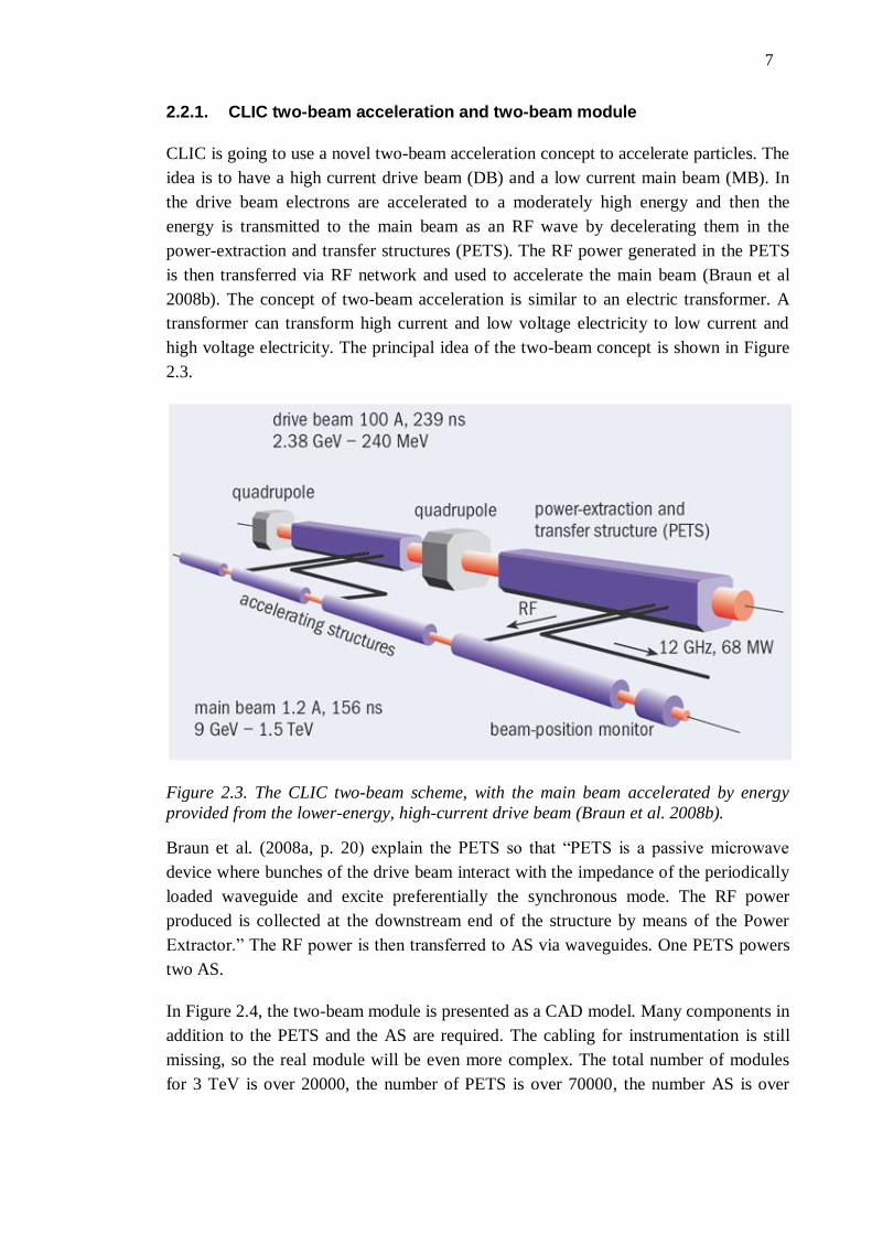
2.2.1. CLIC two-beam acceleration and two-beam module
CLIC is going to use a novel two-beam acceleration concept to accelerate particles. The
idea is to have a high current drive beam (DB) and a low current main beam (MB). In
the drive beam electrons are accelerated to a moderately high energy and then the
energy is transmitted to the main beam as an RF wave by decelerating them in the
power-extraction and transfer structures (PETS). The RF power generated in the PETS
is then transferred via RF network and used to accelerate the main beam (Braun et al
2008b). The concept of two-beam acceleration is similar to an electric transformer. A
transformer can transform high current and low voltage electricity to low current and
high voltage electricity. The principal idea of the two-beam concept is shown in Figure
2.3.
Figure 2.3. The CLIC two-beam scheme, with the main beam accelerated by energy
provided from the lower-energy, high-current drive beam (Braun et al. 2008b).
Braun et al. (2008a, p. 20) explain the PETS so that “PETS is a passive microwave
device where bunches of the drive beam interact with the impedance of the periodically
loaded waveguide and excite preferentially the synchronous mode. The RF power
produced is collected at the downstream end of the structure by means of the Power
Extractor.” The RF power is then transferred to AS via waveguides. One PETS powers
two AS.
In Figure 2.4, the two-beam module is presented as a CAD model. Many components in
addition to the PETS and the AS are required. The cabling for instrumentation is still
missing, so the real module will be even more complex. The total number of modules
for 3 TeV is over 20000, the number of PETS is over 70000, the number AS is over
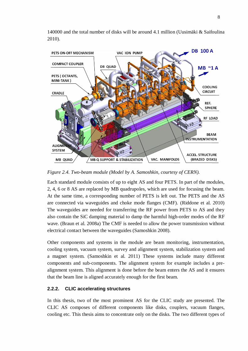
8
140000 and the total number of disks will be around 4.1 million (Uusimäki & Saifoulina
2010).
Figure 2.4. Two-beam module (Model by A. Samoshkin, courtesy of CERN).
Each standard module consists of up to eight AS and four PETS. In part of the modules,
2, 4, 6 or 8 AS are replaced by MB quadrupoles, which are used for focusing the beam.
At the same time, a corresponding number of PETS is left out. The PETS and the AS
are connected via waveguides and choke mode flanges (CMF). (Riddone et al. 2010)
The waveguides are needed for transferring the RF power from PETS to AS and they
also contain the SiC damping material to damp the harmful high-order modes of the RF
wave. (Braun et al. 2008a) The CMF is needed to allow the power transmission without
electrical contact between the waveguides (Samoshkin 2008).
Other components and systems in the module are beam monitoring, instrumentation,
cooling system, vacuum system, survey and alignment system, stabilization system and
a magnet system. (Samoshkin et al. 2011) These systems include many different
components and sub-components. The alignment system for example includes a pre-
alignment system. This alignment is done before the beam enters the AS and it ensures
that the beam line is aligned accurately enough for the first beam.
2.2.2. CLIC accelerating structures
In this thesis, two of the most prominent AS for the CLIC study are presented. The
CLIC AS composes of different components like disks, couplers, vacuum flanges,
cooling etc. This thesis aims to concentrate only on the disks. The two different types of
9
AS are presented in their own sub-chapters 2.2.2.1 and 2.2.2.2. The two different types
of AS are presented because the structure, and the disks in the structure, studied in this
thesis is a test structure and cannot be directly used in CLIC. Thus the second structure
is presented and it is closer to the structure that could be used in CLIC. One AS consists
of multiple disks, usually around 26, which all have different geometry. The disks are
different when a test structure and a fully equipped structure are compared. The two
different types of disks are presented in sub-chapters 2.2.3.1 and 2.2.3.2.
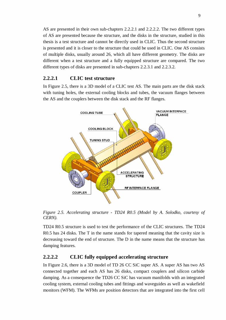
2.2.2.1 CLIC test structure
In Figure 2.5, there is a 3D model of a CLIC test AS. The main parts are the disk stack
with tuning holes, the external cooling blocks and tubes, the vacuum flanges between
the AS and the couplers between the disk stack and the RF flanges.
Figure 2.5. Accelerating structure - TD24 R0.5 (Model by A. Solodko, courtesy of
CERN).
TD24 R0.5 structure is used to test the performance of the CLIC structures. The TD24
R0.5 has 24 disks. The T in the name stands for tapered meaning that the cavity size is
decreasing toward the end of structure. The D in the name means that the structure has
damping features.
2.2.2.2 CLIC fully equipped accelerating structure
In Figure 2.6, there is a 3D model of TD 26 CC SiC super AS. A super AS has two AS
connected together and each AS has 26 disks, compact couplers and silicon carbide
damping. As a consequence the TD26 CC SiC has vacuum manifolds with an integrated
cooling system, external cooling tubes and fittings and waveguides as well as wakefield
monitors (WFM). The WFMs are position detectors that are integrated into the first cell
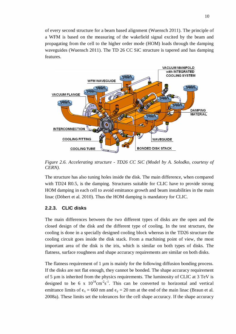
10
of every second structure for a beam based alignment (Wuensch 2011). The principle of
a WFM is based on the measuring of the wakefield signal excited by the beam and
propagating from the cell to the higher order mode (HOM) loads through the damping
waveguides (Wuensch 2011). The TD 26 CC SiC structure is tapered and has damping
features.
Figure 2.6. Accelerating structure - TD26 CC SiC (Model by A. Solodko, courtesy of
CERN).
The structure has also tuning holes inside the disk. The main difference, when compared
with TD24 R0.5, is the damping. Structures suitable for CLIC have to provide strong
HOM damping in each cell to avoid emittance growth and beam instabilities in the main
linac (Döbert et al. 2010). Thus the HOM damping is mandatory for CLIC.
2.2.3. CLIC disks
The main differences between the two different types of disks are the open and the
closed design of the disk and the different type of cooling. In the test structure, the
cooling is done in a specially designed cooling block whereas in the TD26 structure the
cooling circuit goes inside the disk stack. From a machining point of view, the most
important area of the disk is the iris, which is similar on both types of disks. The
flatness, surface roughness and shape accuracy requirements are similar on both disks.
The flatness requirement of 1 µm is mainly for the following diffusion bonding process.
If the disks are not flat enough, they cannot be bonded. The shape accuracy requirement
of 5 µm is inherited from the physics requirements. The luminosity of CLIC at 3 TeV is
designed to be 6 x 1034
cm-2
s-1
. This can be converted to horizontal and vertical
emittance limits of ϵx = 660 nm and ϵy = 20 nm at the end of the main linac (Braun et al.
2008a). These limits set the tolerances for the cell shape accuracy. If the shape accuracy
11
is not under 5 µm, this will cause dephasing (Zennaro 2008b). Dephasing means that the
timing of the accelerating wave is not correct with regard to the particle bunch. This will
have a negative effect on the luminosity. The surface roughness Ra 25 nm requirement
is due to the RF requirements. During the operation of the AS, the structure is subject to
high magnetic and electric fields. The surface roughness has an effect on the arc
generation (Atieh et al. 2011). The smoother the surface is the less breakdowns and arcs
the AS is to experience. The tolerances of the disks are defined in their respective CAD
drawings. In Appendix 1, there is a complete CAD drawing for one of the disks. The
notation in the drawings is according to ISO 1101.
The tuning holes are used to tune the structure to nominal frequency. The tuning of a
structure is done by deforming the inner wall of the disk. The walls can be either pushed
in or pulled out by a few µm. The tuning process is very time consuming because at the
moment it is done manually and each disk has four tuning holes which can be used. For
the AS, which will be installed in CLIC, tuning is not considered due to the very large
number of AS and the huge amount of work it would require, but for testing in the early
phases of manufacturing, it is suitable. The biggest difference is in the machining of the
shapes near the outer walls of the disk because the TD26 disk has an open slot there (see
Figure 2.8) and the TD24 test disk has closed wall (see Figure 2.7).
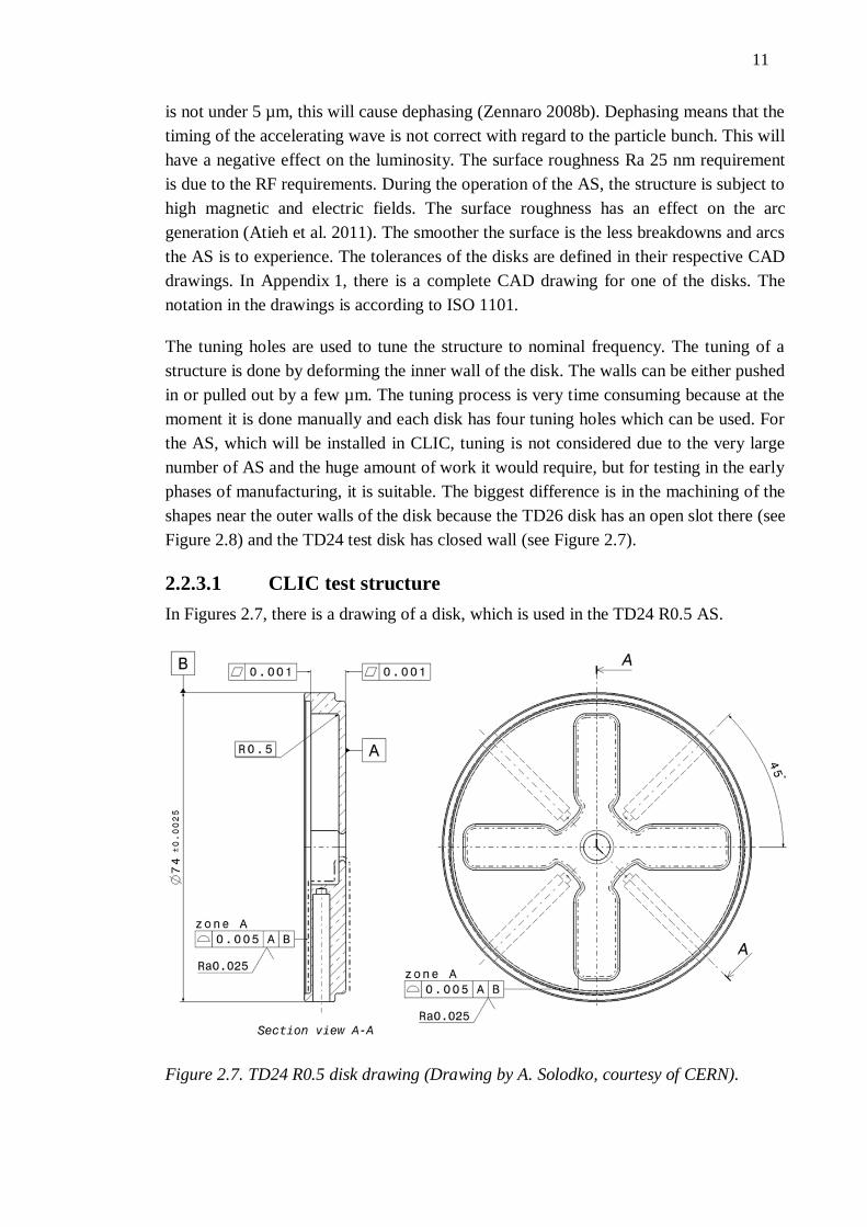
2.2.3.1 CLIC test structure
In Figures 2.7, there is a drawing of a disk, which is used in the TD24 R0.5 AS.
Figure 2.7. TD24 R0.5 disk drawing (Drawing by A. Solodko, courtesy of CERN).
12
R0.5 in the name means that the edge radius of the disk cavity wall is 0.5 mm, otherwise
the cutting tool would need to be changed to one with a smaller radius during milling.
This also reduces pulse surface heating (Wuensch 2011). The disk has tuning holes.
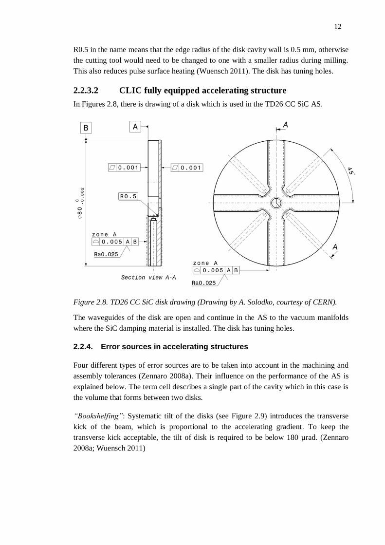
2.2.3.2 CLIC fully equipped accelerating structure
In Figures 2.8, there is drawing of a disk which is used in the TD26 CC SiC AS.
Figure 2.8. TD26 CC SiC disk drawing (Drawing by A. Solodko, courtesy of CERN).
The waveguides of the disk are open and continue in the AS to the vacuum manifolds
where the SiC damping material is installed. The disk has tuning holes.
2.2.4. Error sources in accelerating structures
Four different types of error sources are to be taken into account in the machining and
assembly tolerances (Zennaro 2008a). Their influence on the performance of the AS is
explained below. The term cell describes a single part of the cavity which in this case is
the volume that forms between two disks.
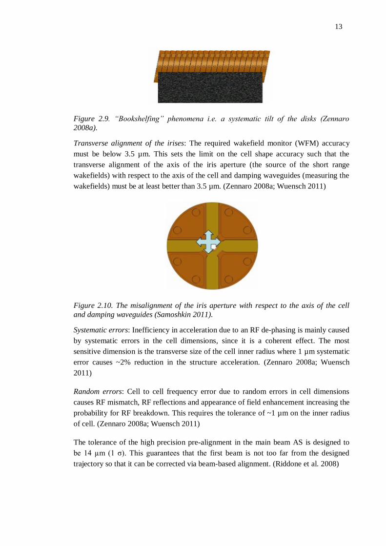
“Bookshelfing”: Systematic tilt of the disks (see Figure 2.9) introduces the transverse
kick of the beam, which is proportional to the accelerating gradient. To keep the
transverse kick acceptable, the tilt of disk is required to be below 180 µrad. (Zennaro
2008a; Wuensch 2011)
13
Figure 2.9. “Bookshelfing” phenomena i.e. a systematic tilt of the disks (Zennaro
2008a).
Transverse alignment of the irises: The required wakefield monitor (WFM) accuracy
must be below 3.5 µm. This sets the limit on the cell shape accuracy such that the
transverse alignment of the axis of the iris aperture (the source of the short range
wakefields) with respect to the axis of the cell and damping waveguides (measuring the
wakefields) must be at least better than 3.5 µm. (Zennaro 2008a; Wuensch 2011)
Figure 2.10. The misalignment of the iris aperture with respect to the axis of the cell
and damping waveguides (Samoshkin 2011).
Systematic errors: Inefficiency in acceleration due to an RF de-phasing is mainly caused
by systematic errors in the cell dimensions, since it is a coherent effect. The most
sensitive dimension is the transverse size of the cell inner radius where 1 µm systematic
error causes ~2% reduction in the structure acceleration. (Zennaro 2008a; Wuensch
2011)
Random errors: Cell to cell frequency error due to random errors in cell dimensions
causes RF mismatch, RF reflections and appearance of field enhancement increasing the
probability for RF breakdown. This requires the tolerance of ~1 µm on the inner radius
of cell. (Zennaro 2008a; Wuensch 2011)
The tolerance of the high precision pre-alignment in the main beam AS is designed to
be 14 µm (1 σ). This guarantees that the first beam is not too far from the designed
trajectory so that it can be corrected via beam-based alignment. (Riddone et al. 2008)
14
3. MANUFACTURING AN ACCELERATING
STRUCTURE AND A DISK
This chapter gives a brief overview on how the AS used in the two-beam modules are
manufactured. A particular emphasis is given to the disks and more specifically to a
single manufacturing step of ultra high precision machining. The term manufacturing
refers to the process of making an AS or a disk from raw materials or parts. Machining
on the other hand refers to a process of doing mechanical work to shape a workpiece,
for example a disk, to match the drawing. Thus machining is one part of the
manufacturing process. The scope of this thesis is limited to a single manufacturing step
of an AS, namely the ultra precision machining of a disk. The manufacturing of an AS
is only taken into account in the cost considerations in chapter 6. The manufacturing
costs other than ultra precision machining are taken from the previous studies.
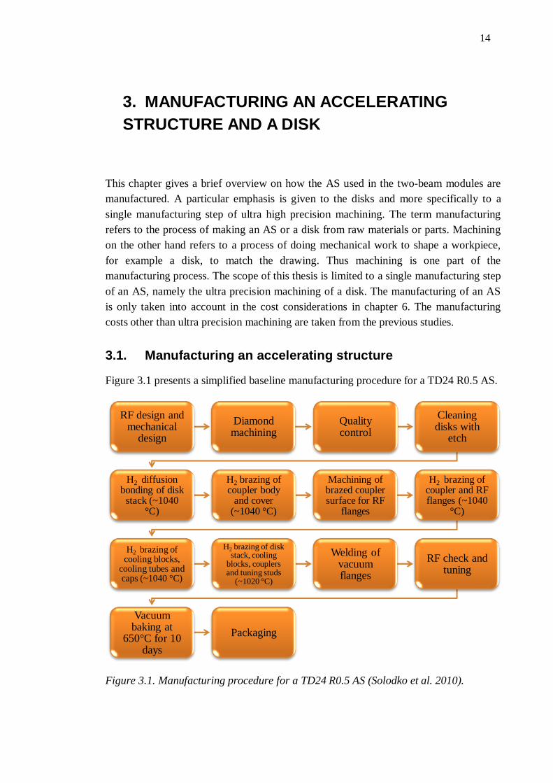
3.1. Manufacturing an accelerating structure
Figure 3.1 presents a simplified baseline manufacturing procedure for a TD24 R0.5 AS.
Figure 3.1. Manufacturing procedure for a TD24 R0.5 AS (Solodko et al. 2010).
RF design and mechanical
design
Diamond machining
Quality control
Cleaning disks with
etch
H2 diffusion bonding of disk
stack (~1040 °C)
H2 brazing of coupler body
and cover (~1040 °C)
Machining of brazed coupler surface for RF
flanges
H2 brazing of coupler and RF flanges (~1040
°C)
H2 brazing of cooling blocks,
cooling tubes and caps (~1040 °C)
H2 brazing of disk stack, cooling
blocks, couplers and tuning studs
(~1020 °C)
Welding of vacuum flanges
RF check and tuning
Vacuum baking at
650°C for 10 days
Packaging
15
All of the steps in the manufacturing procedure are carefully defined and tested.
Furthermore, new methods are continuously being explored. The manufacturing
procedure starts with an RF design. The desired physics properties of the AS are defined
at this stage. Based on the physics requirements, a 3D model of the AS is designed in
CAD software. In this phase, the mechanical structure of the AS as well as the
interfaces between the AS and other systems will be designed. After the model is
designed then the appropriate 2D drawings for different parts and components are
produced. Some parts are standard so they can be purchased for the assembly; others
need to be manufactured according to the drawings.
The first step after design is the diamond machining of the disks. The disks are then
taken through quality control. The quality control involves an inlet inspection,
dimensional control, possibly scanning electron microscope (SEM) micrographs and a
preliminary RF check to evaluate the scattering parameters and the possibility of tuning.
The disks are then etched and bonded to a disk stack. All bonding and brazing steps take
place under H2 atmosphere.
First brazing step is the brazing of a coupler body and cover together. The coupler
surface is then machined before brazing RF flanges to the coupler. A cooling block,
tubes and caps are brazed together. The disk stack, the cooling blocks, couplers, beam
pipes and tuning studs are then brazed together followed by the welding of vacuum
flanges to the AS. After that an RF check and tuning are done to the structure. Finally
the AS is baked for 10 days in a vacuum at 650 °C to remove the hydrogen in the AS.
The baseline manufacturing procedure presented in Figure 3.1 is a simplified version of
the total process. Depending on the AS design the manufacturing flow can have more or
less steps than presented in Figure 3.1.
3.2. Manufacturing a disk
In chapter 3.2, a brief overview of the methods used for manufacturing a disk is given.
The manufacturing steps include phases such as machining and heat treatments. The
machining methods include turning and milling while the measurement methods include
contact and non-contact methods. The measured parameters are presented in chapter 4
Geometrical measurements.
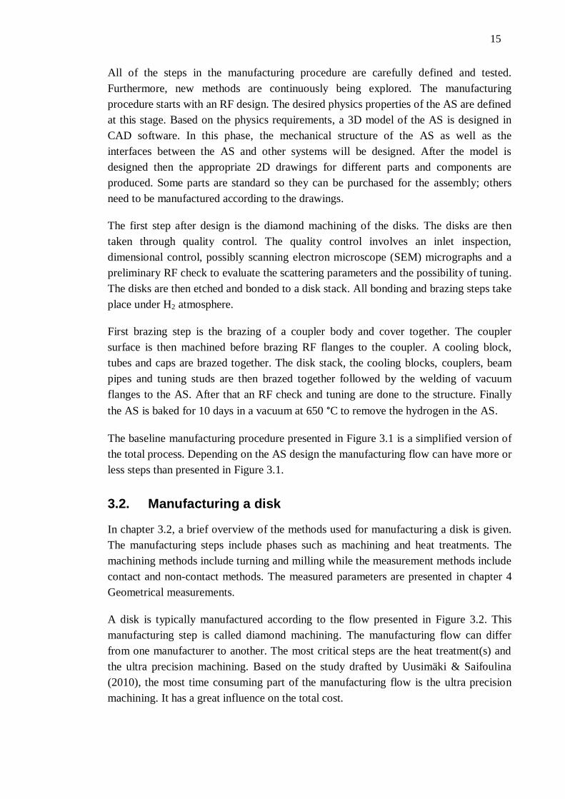
A disk is typically manufactured according to the flow presented in Figure 3.2. This
manufacturing step is called diamond machining. The manufacturing flow can differ
from one manufacturer to another. The most critical steps are the heat treatment(s) and
the ultra precision machining. Based on the study drafted by Uusimäki & Saifoulina
(2010), the most time consuming part of the manufacturing flow is the ultra precision
machining. It has a great influence on the total cost.
16
Figure 3.2. A typical flow for machining of a disk (Machining flow by S. Atieh).
At first the copper is inspected and then cut to disks. The disks are then pre-machined to
a shape leaving roughly 100 µm of extra material on the disks. A heat treatment is done
after the pre-machining in order to reduce the stress in material. This is followed by
precise machining leaving around 10 µm of extra material on the disks. The second
stress relief is done after precise machining. The ultra precision milling and turning will
follow. Multiple machining steps are needed to keep the depth of cut small enough. In
the end, the disks are degreased and taken through quality control. An example of a
more specific and validated machining flow of a disk can be found in Appendix 2.
3.2.1. Material
The material used for the disks is copper. The alloy is oxygen-free electrolytic (OFE)
copper. The copper is multidirectional forged and contains at least 99.99% copper. The
other chemical elements allowed in the alloy are oxygen (max. 0.0005%) and 16 other
named elements. OFE copper is the alloy C10100 according to the Unified Numbering
System (UNS). The grain size is fine (max. 90 µm) and homogenous. (Atieh et al. 2011,
CDA 2011) The OFE copper has a conductivity of at least 101% with respect to the
International Annealed Copper Standard (IACS). The standard was adopted in 1913 so
Inspection of material
Cutting raw material to
disks Stress relief Pre-machining
Stress relief Precise
machining Stress relief
Ultra precision machining
Degreasing Quality control
17
some of the today’s commercial pure copper products have values above 100%. (CDA
2011)
Machinability is defined as the relative ease or difficult whereby given metal can be
machined (Grzesik 2008). Usually, machinability is tested with respect to tool life or
wear, surface finish, cutting force, power consumption or cutting temperature. Among
different types of copper and copper alloys, OFE copper is in the group of difficult-to-
machine alloys. The alloys in this group are the hardest to machine among copper
alloys. Those copper alloys in the group of difficult-to-machine alloys that contain more
oxygen are easier to machine than OFE due to the fact that the cuprous oxide facilitates
chip breakage. The coppers containing oxygen are better in machinability, type of chip,
and surface finish than oxygen-free copper. (ASM International Handbook Committee
1989) For OFE copper the machining process needs to be well defined and known.
3.2.2. Machining techniques
The disks are machined by milling and turning. The machining phases include all steps
from pre-machining to ultra precise finishing.
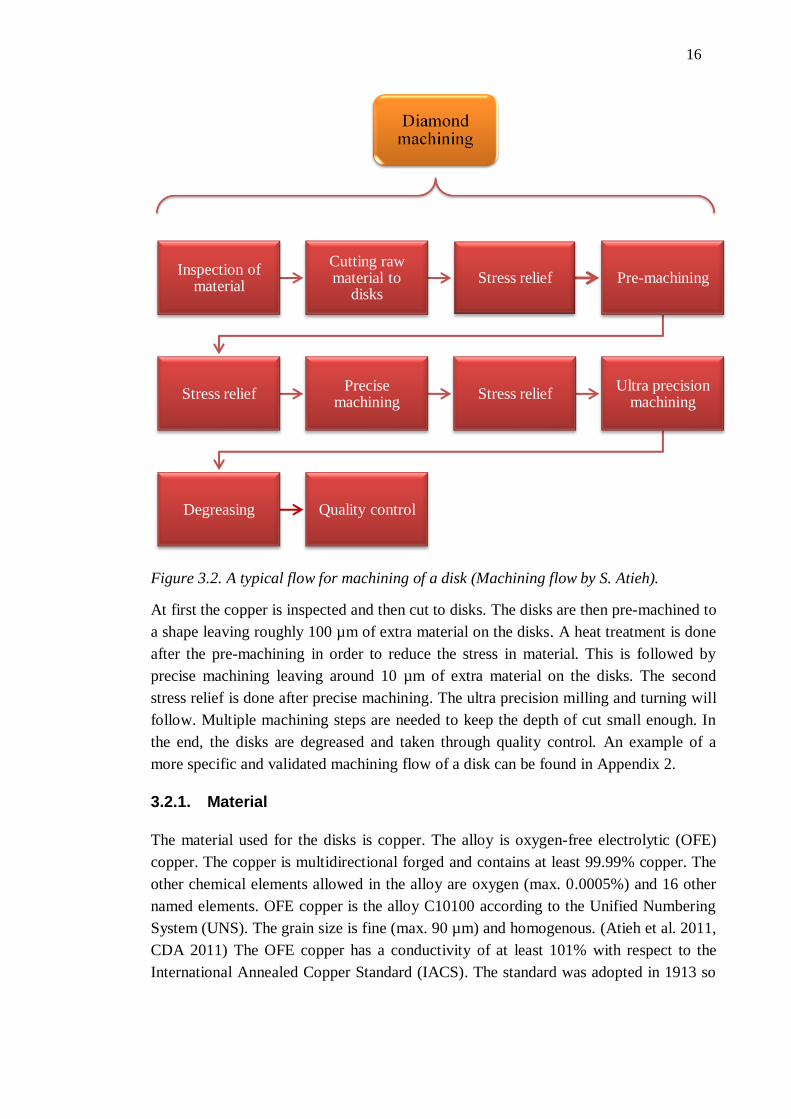
3.2.2.1 Conventional milling
Milling is a machine process that enables the machining of more complex forms than
turning. A milling tool often has more than one cutting teeth (Black et al. 1996). In
milling, the tool usually rotates around its axis and at the same time the tool is feed into
a stationary workpiece (or a workpiece is feed into a tool) (Black et al. 1996). A typical
milling setup is represented in Figure 3.3.
Figure 3.3. Milling (CustomPartNet 2007).
18
A milling machine can house many different types of milling tools depending on the
milling method and the desired form.
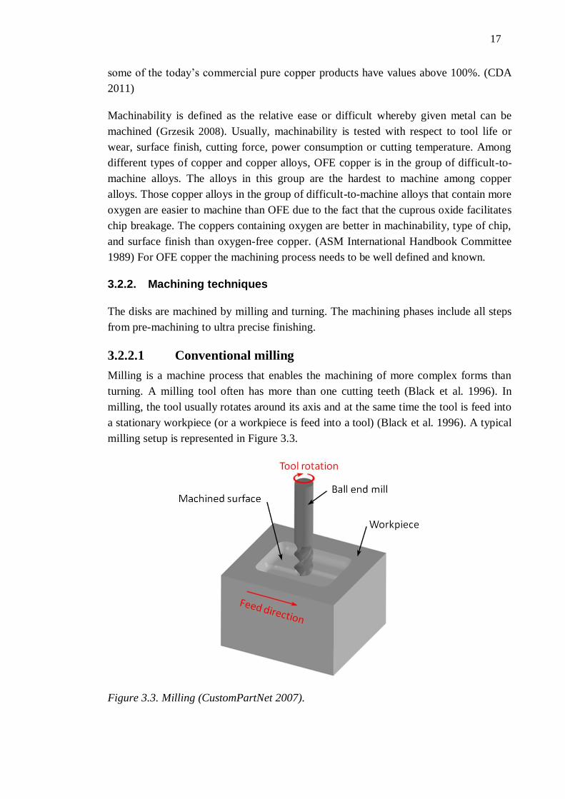
3.2.2.2 Conventional turning
Turning is one of the basic mechanisms for machining metals and other solid materials.
It generates cylindrical forms with a single point tool and the tool is usually stationary
while the workpiece is rotating (Black et al. 1996). A typical turning setup is shown in
Figure 3.4.
Figure 3.4. Turning (CustomPartNet 2007).
The feed movement of a turning tool can be along the axis of the workpiece or
alternatively the tool can be feed in the radial direction of the workpiece (Black et al.
1996).
3.2.3. Need of ultra precision machining
The term nanotechnology was coined by Norio Taguchi in 1974 to term precision
machining with a tolerance of a micron or less. The term nanotechnology means that the
structure of the material has come down to a few atoms. One nanometre can house
between 4 and 20 atoms depending on the size of the atom. Thus ultra precise
machining means removing material to achieve structures, which are in a precision of
only few hundreds of atoms. To distinguish ultra precise machining from precise and
fine machining a categorisation like the one in Figure 3.5 can be used.
19
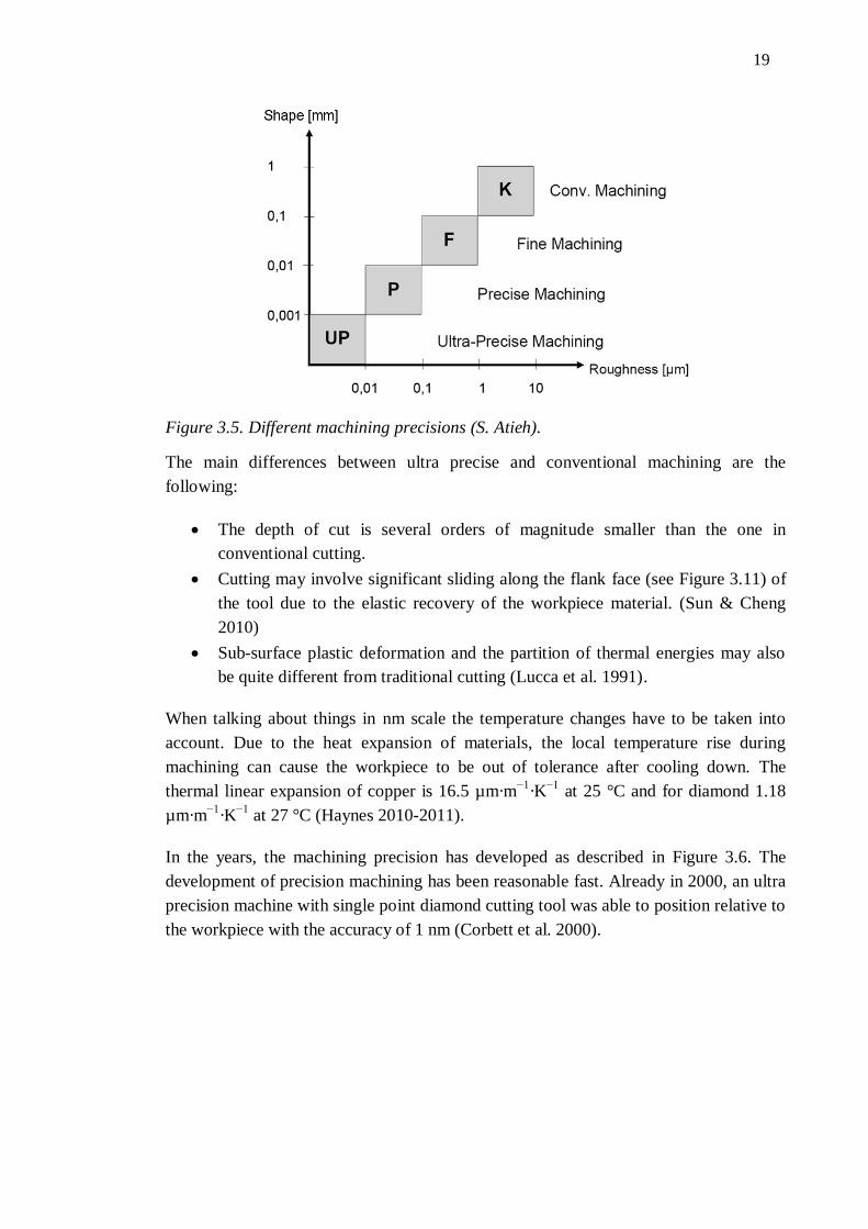
Figure 3.5. Different machining precisions (S. Atieh).
The main differences between ultra precise and conventional machining are the
following:
The depth of cut is several orders of magnitude smaller than the one in
conventional cutting.
Cutting may involve significant sliding along the flank face (see Figure 3.11) of
the tool due to the elastic recovery of the workpiece material. (Sun & Cheng
2010)
Sub-surface plastic deformation and the partition of thermal energies may also
be quite different from traditional cutting (Lucca et al. 1991).
When talking about things in nm scale the temperature changes have to be taken into
account. Due to the heat expansion of materials, the local temperature rise during
machining can cause the workpiece to be out of tolerance after cooling down. The
thermal linear expansion of copper is 16.5 µm·m−1
·K−1
at 25 °C and for diamond 1.18
µm·m−1
·K−1
at 27 °C (Haynes 2010-2011).
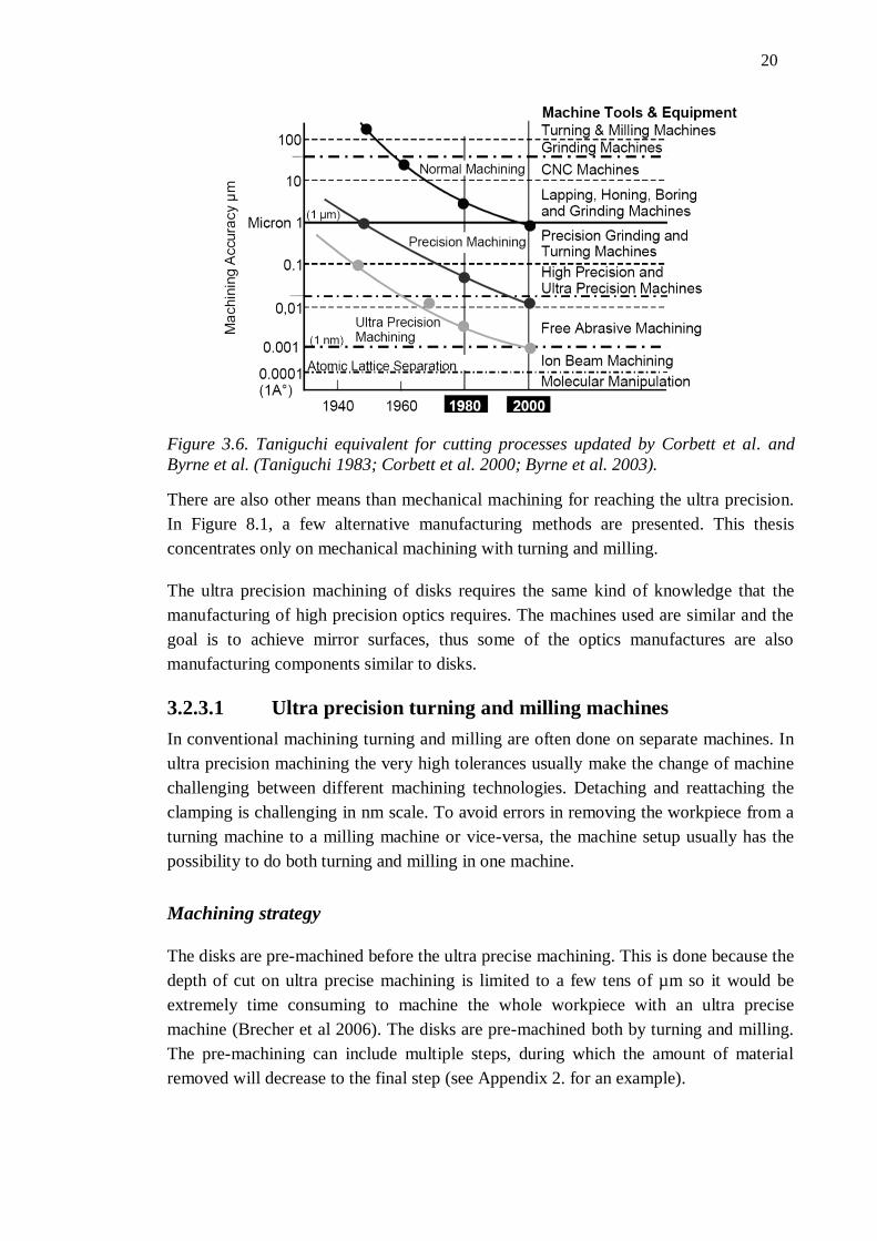
In the years, the machining precision has developed as described in Figure 3.6. The
development of precision machining has been reasonable fast. Already in 2000, an ultra
precision machine with single point diamond cutting tool was able to position relative to
the workpiece with the accuracy of 1 nm (Corbett et al. 2000).
20
Figure 3.6. Taniguchi equivalent for cutting processes updated by Corbett et al. and
Byrne et al. (Taniguchi 1983; Corbett et al. 2000; Byrne et al. 2003).
There are also other means than mechanical machining for reaching the ultra precision.
In Figure 8.1, a few alternative manufacturing methods are presented. This thesis
concentrates only on mechanical machining with turning and milling.
The ultra precision machining of disks requires the same kind of knowledge that the
manufacturing of high precision optics requires. The machines used are similar and the
goal is to achieve mirror surfaces, thus some of the optics manufactures are also
manufacturing components similar to disks.
3.2.3.1 Ultra precision turning and milling machines
In conventional machining turning and milling are often done on separate machines. In
ultra precision machining the very high tolerances usually make the change of machine
challenging between different machining technologies. Detaching and reattaching the
clamping is challenging in nm scale. To avoid errors in removing the workpiece from a
turning machine to a milling machine or vice-versa, the machine setup usually has the
possibility to do both turning and milling in one machine.
Machining strategy
The disks are pre-machined before the ultra precise machining. This is done because the
depth of cut on ultra precise machining is limited to a few tens of µm so it would be
extremely time consuming to machine the whole workpiece with an ultra precise
machine (Brecher et al 2006). The disks are pre-machined both by turning and milling.
The pre-machining can include multiple steps, during which the amount of material
removed will decrease to the final step (see Appendix 2. for an example).
21
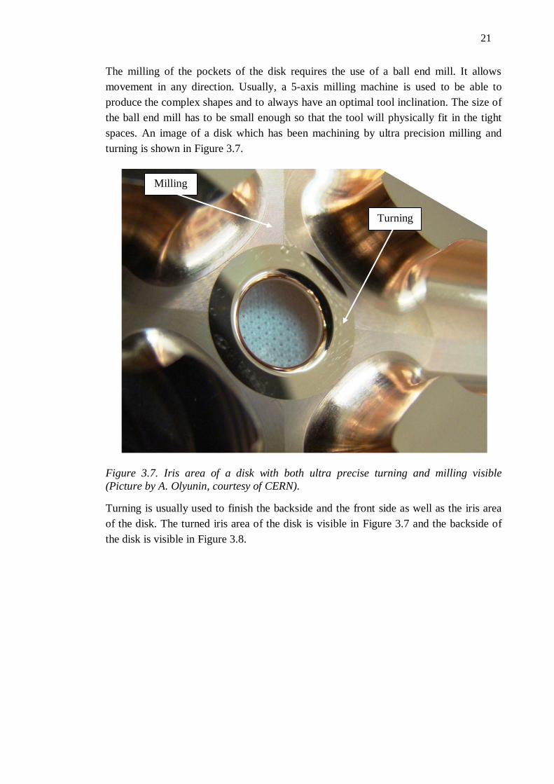
The milling of the pockets of the disk requires the use of a ball end mill. It allows
movement in any direction. Usually, a 5-axis milling machine is used to be able to
produce the complex shapes and to always have an optimal tool inclination. The size of
the ball end mill has to be small enough so that the tool will physically fit in the tight
spaces. An image of a disk which has been machining by ultra precision milling and
turning is shown in Figure 3.7.
Figure 3.7. Iris area of a disk with both ultra precise turning and milling visible
(Picture by A. Olyunin, courtesy of CERN).
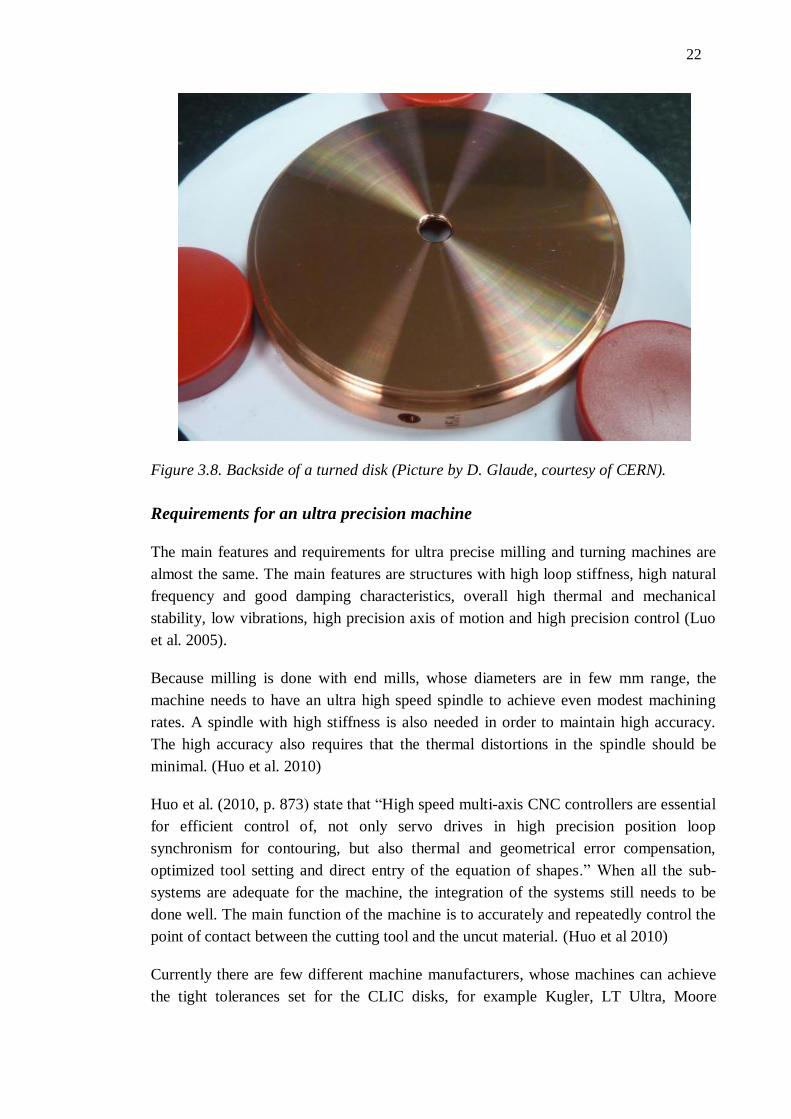
Turning is usually used to finish the backside and the front side as well as the iris area
of the disk. The turned iris area of the disk is visible in Figure 3.7 and the backside of
the disk is visible in Figure 3.8.
Turning
Milling
22
Figure 3.8. Backside of a turned disk (Picture by D. Glaude, courtesy of CERN).
Requirements for an ultra precision machine
The main features and requirements for ultra precise milling and turning machines are
almost the same. The main features are structures with high loop stiffness, high natural
frequency and good damping characteristics, overall high thermal and mechanical
stability, low vibrations, high precision axis of motion and high precision control (Luo
et al. 2005).
Because milling is done with end mills, whose diameters are in few mm range, the
machine needs to have an ultra high speed spindle to achieve even modest machining
rates. A spindle with high stiffness is also needed in order to maintain high accuracy.
The high accuracy also requires that the thermal distortions in the spindle should be
minimal. (Huo et al. 2010)
Huo et al. (2010, p. 873) state that “High speed multi-axis CNC controllers are essential
for efficient control of, not only servo drives in high precision position loop
synchronism for contouring, but also thermal and geometrical error compensation,
optimized tool setting and direct entry of the equation of shapes.” When all the sub-
systems are adequate for the machine, the integration of the systems still needs to be
done well. The main function of the machine is to accurately and repeatedly control the
point of contact between the cutting tool and the uncut material. (Huo et al 2010)
Currently there are few different machine manufacturers, whose machines can achieve
the tight tolerances set for the CLIC disks, for example Kugler, LT Ultra, Moore
23
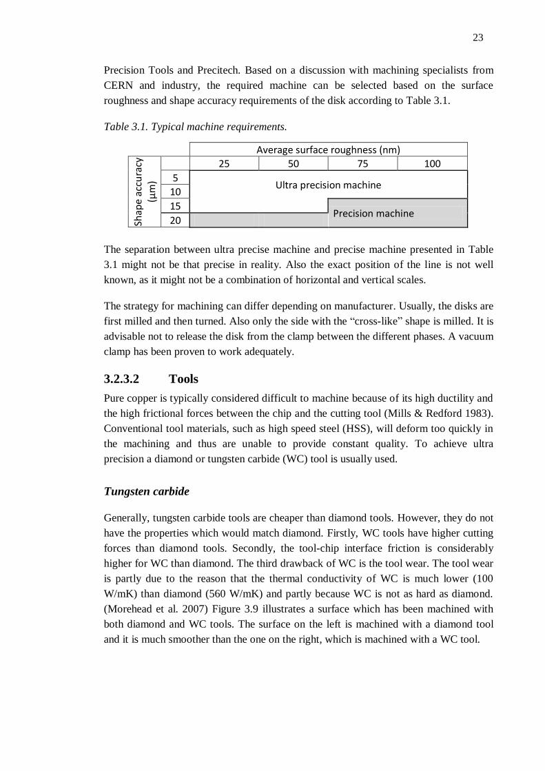
Precision Tools and Precitech. Based on a discussion with machining specialists from
CERN and industry, the required machine can be selected based on the surface
roughness and shape accuracy requirements of the disk according to Table 3.1.
Table 3.1. Typical machine requirements.
Average surface roughness (nm)
Shap
e ac
cura
cy
(µm
) 25 50 75 100
5 Ultra precision machine
10
15 Precision machine
20
The separation between ultra precise machine and precise machine presented in Table
3.1 might not be that precise in reality. Also the exact position of the line is not well
known, as it might not be a combination of horizontal and vertical scales.
The strategy for machining can differ depending on manufacturer. Usually, the disks are
first milled and then turned. Also only the side with the “cross-like” shape is milled. It is
advisable not to release the disk from the clamp between the different phases. A vacuum
clamp has been proven to work adequately.
3.2.3.2 Tools
Pure copper is typically considered difficult to machine because of its high ductility and
the high frictional forces between the chip and the cutting tool (Mills & Redford 1983).
Conventional tool materials, such as high speed steel (HSS), will deform too quickly in
the machining and thus are unable to provide constant quality. To achieve ultra
precision a diamond or tungsten carbide (WC) tool is usually used.
Tungsten carbide
Generally, tungsten carbide tools are cheaper than diamond tools. However, they do not
have the properties which would match diamond. Firstly, WC tools have higher cutting
forces than diamond tools. Secondly, the tool-chip interface friction is considerably
higher for WC than diamond. The third drawback of WC is the tool wear. The tool wear
is partly due to the reason that the thermal conductivity of WC is much lower (100
W/mK) than diamond (560 W/mK) and partly because WC is not as hard as diamond.
(Morehead et al. 2007) Figure 3.9 illustrates a surface which has been machined with
both diamond and WC tools. The surface on the left is machined with a diamond tool
and it is much smoother than the one on the right, which is machined with a WC tool.
24
Figure 3.9. Surfaces machined by a diamond tool on the left and by a WC tool on the
right (SEM micrographs by G. Arnau, courtesy of CERN).
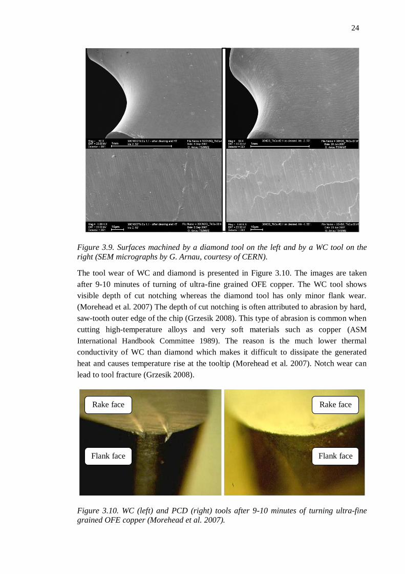
The tool wear of WC and diamond is presented in Figure 3.10. The images are taken
after 9-10 minutes of turning of ultra-fine grained OFE copper. The WC tool shows
visible depth of cut notching whereas the diamond tool has only minor flank wear.
(Morehead et al. 2007) The depth of cut notching is often attributed to abrasion by hard,
saw-tooth outer edge of the chip (Grzesik 2008). This type of abrasion is common when
cutting high-temperature alloys and very soft materials such as copper (ASM
International Handbook Committee 1989). The reason is the much lower thermal
conductivity of WC than diamond which makes it difficult to dissipate the generated
heat and causes temperature rise at the tooltip (Morehead et al. 2007). Notch wear can
lead to tool fracture (Grzesik 2008).
Figure 3.10. WC (left) and PCD (right) tools after 9-10 minutes of turning ultra-fine
grained OFE copper (Morehead et al. 2007).
Flank face Flank face
Rake face Rake face
25
Filiz et al. (2007) conducted wide milling tests with OFE copper and tungsten carbide
tools. They found out that the best average surface roughness Ra they could achieve was
just under 100 nm. They also noticed that the achieved values differ quite much from
the theoretical ones. (Filiz et al. 2007) This value agrees with the one presented in Table
3.2. It is still unknown if a lower average surface roughness Ra than 100 nm can be
achieved in milling with WC tools. Huo and Cheng achieved (2010) surface roughness
Ra of 24 nm while slot milling OFE copper with two-fluted WC micro end mill.
However, they only generated straight slots in their test and measured the surface
roughness Ra along the milling direction at the bottom of slot. In similar conditions,
similarly sized one-fluted CVD and natural diamond end mills produced 13 and 11 nm
surface roughness Ra (Huo & Cheng 2010). Turning OFE copper with polycrystalline
diamond (PCD) tool yielded half the surface roughness compared with a WC tool
(Morehead et al. 2007).
Diamond
Diamond is used for tools because of its good properties regarding metal machining. It
has a low coefficient of friction and thermal expansion, high strength and resistance to
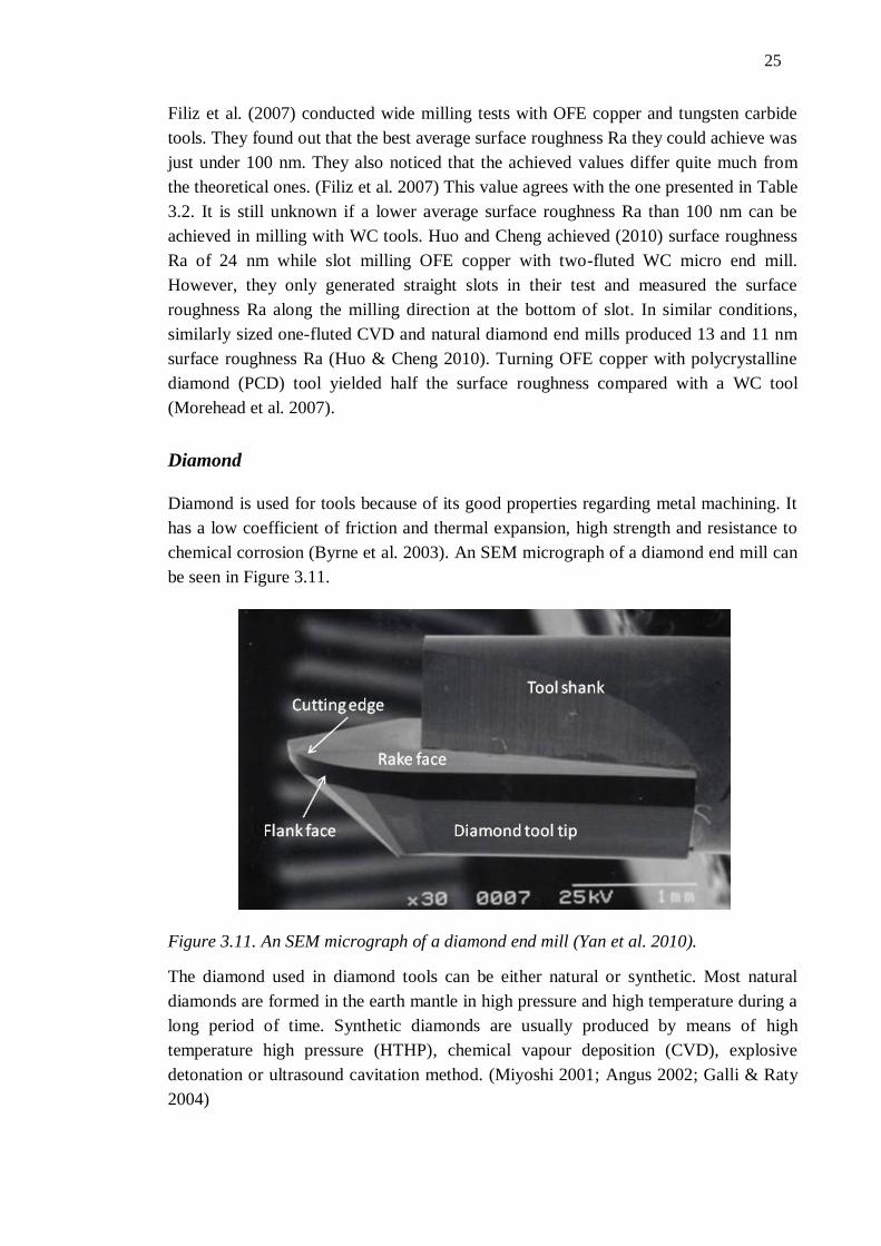
chemical corrosion (Byrne et al. 2003). An SEM micrograph of a diamond end mill can
be seen in Figure 3.11.
Figure 3.11. An SEM micrograph of a diamond end mill (Yan et al. 2010).
The diamond used in diamond tools can be either natural or synthetic. Most natural
diamonds are formed in the earth mantle in high pressure and high temperature during a
long period of time. Synthetic diamonds are usually produced by means of high
temperature high pressure (HTHP), chemical vapour deposition (CVD), explosive
detonation or ultrasound cavitation method. (Miyoshi 2001; Angus 2002; Galli & Raty
2004)
26
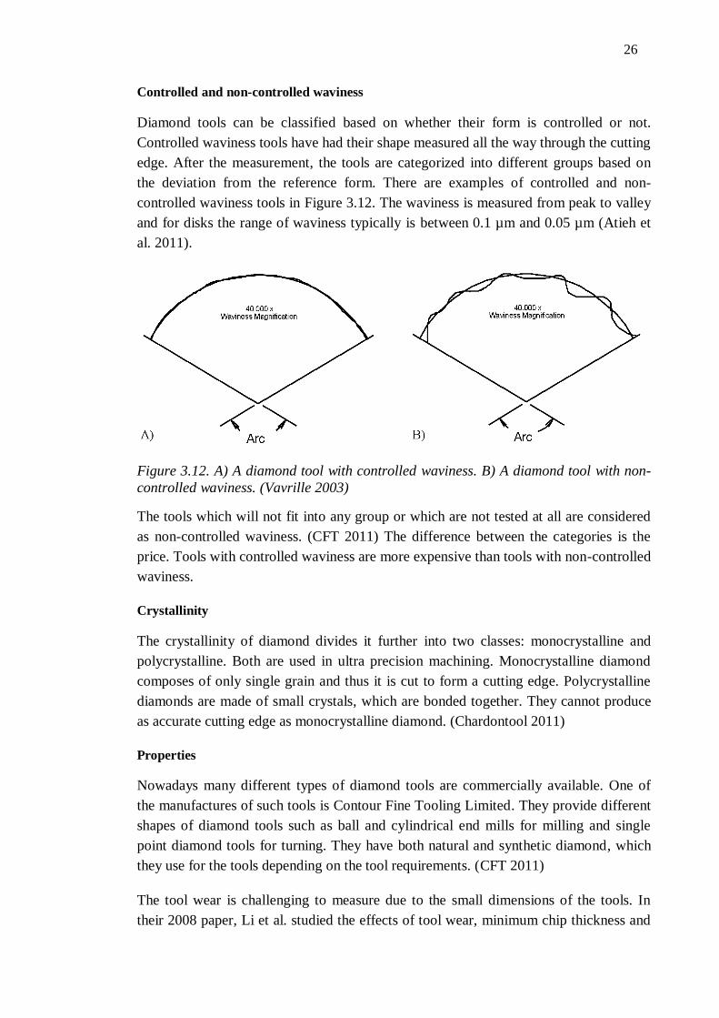
Controlled and non-controlled waviness
Diamond tools can be classified based on whether their form is controlled or not.
Controlled waviness tools have had their shape measured all the way through the cutting
edge. After the measurement, the tools are categorized into different groups based on
the deviation from the reference form. There are examples of controlled and non-
controlled waviness tools in Figure 3.12. The waviness is measured from peak to valley
and for disks the range of waviness typically is between 0.1 µm and 0.05 µm (Atieh et
al. 2011).
Figure 3.12. A) A diamond tool with controlled waviness. B) A diamond tool with non-
controlled waviness. (Vavrille 2003)
The tools which will not fit into any group or which are not tested at all are considered
as non-controlled waviness. (CFT 2011) The difference between the categories is the
price. Tools with controlled waviness are more expensive than tools with non-controlled
waviness.
Crystallinity
The crystallinity of diamond divides it further into two classes: monocrystalline and
polycrystalline. Both are used in ultra precision machining. Monocrystalline diamond
composes of only single grain and thus it is cut to form a cutting edge. Polycrystalline
diamonds are made of small crystals, which are bonded together. They cannot produce
as accurate cutting edge as monocrystalline diamond. (Chardontool 2011)
Properties
Nowadays many different types of diamond tools are commercially available. One of
the manufactures of such tools is Contour Fine Tooling Limited. They provide different
shapes of diamond tools such as ball and cylindrical end mills for milling and single
point diamond tools for turning. They have both natural and synthetic diamond, which
they use for the tools depending on the tool requirements. (CFT 2011)
The tool wear is challenging to measure due to the small dimensions of the tools. In
their 2008 paper, Li et al. studied the effects of tool wear, minimum chip thickness and
27
tool geometry on the surface roughness. They used oxygen free high conducting copper
in their tests. Their remarks are that the cutting velocity and material removal volume
have great influence on tool wear. The higher speed causes faster tool wear, which in
turn increases the surface roughness. The depth of cut and feed per tooth have very little
effect on tool wear. (Li et al. 2008) Many studies have showed that cutting velocity has
great influence on the tool wear (Medicus et al. 2007; Jawaid et al. 2000, Teitenberg et
al. 1992). A diamond tool can be used to cut nonferrous metals such as aluminium and
copper for a distance up to a few hundreds of kilometres (Hamada 1985 cited by Yan et
al. 2003). According to Yan et al. (2010) the tool wear is insignificant when machining
OFE copper with a single-crystalline diamond ball end mill.
Based on a discussion with the ultra precision machining specialists from CERN and
industry, Table 3.2 was drafted to describe the different types of tools required with
different surface roughness and shape accuracy requirements.
Table 3.2. Typical requirements for tools.
Average surface roughness (nm)
Shap
e ac
cura
cy
(µm
)
25 50 75 100
5
Monocrystalline diamond Monocrystalline diamond
10
15 Non-controlled diamond
Polycrystalline diamond/carbide 20
Table 3.2 exhibits the same reasoning for the borders as did Table 3.1. Technology
advances fast in this field of science, so the borders also evolve in time.
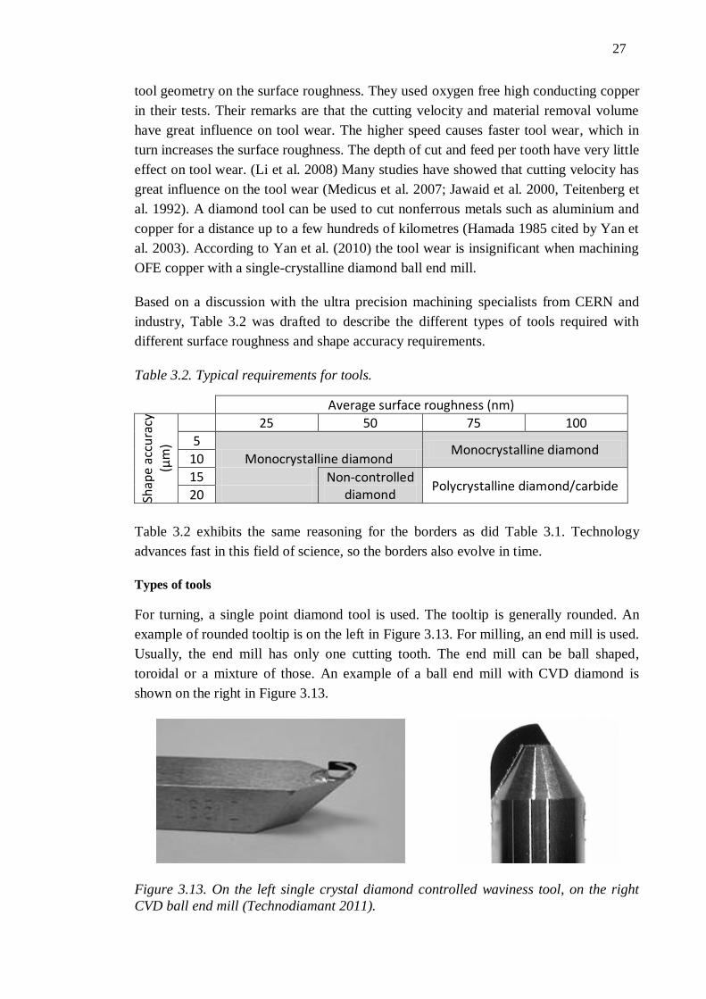
Types of tools
For turning, a single point diamond tool is used. The tooltip is generally rounded. An
example of rounded tooltip is on the left in Figure 3.13. For milling, an end mill is used.
Usually, the end mill has only one cutting tooth. The end mill can be ball shaped,
toroidal or a mixture of those. An example of a ball end mill with CVD diamond is
shown on the right in Figure 3.13.
Figure 3.13. On the left single crystal diamond controlled waviness tool, on the right
CVD ball end mill (Technodiamant 2011).
28
A CAD drawing of a single crystal diamond end mill can be seen in Appendix 3.
3.2.4. Heat treatments
Heat treatment is a process during which the temperature of the material is raised above
the normal temperature. This is done in order to homogenize the material, release the
internal stress of the material and to improve the machinability of the material. Heat
treatment can be divided into two processes: annealing and stress relief. (Chandler
1996; ASM International Handbook Committee 1991) Sometimes the term annealing
can be used to represent all heat treatment methods. In this thesis, the stress relief and
the annealing are considered as different processes.
During the processing or fabrication of copper the plastic strain is increased. Because
plastic strain is accompanied by elastic strain, residual stresses remain in the workpiece
and this can result in unwanted cracking or in unpredictable distortions. The cracking
and distortions can occur during cutting or machining as well as during brazing, welding
and bonding. The heat treatments for stress relief are carried out to reduce this stress. A
typical temperature for OFE copper is around 180 °C. A relatively small surface
residual stress value can be achieved by stress relief between pre-machining and ultra
precision diamond machining. (Geng 2004; Zhang & Zhang 1994; ASM International
Handbook Committee 1991) In the disks, the plastic strain is caused by the forging of
copper and the pre-machining. The ultra precision machining itself has so low forces
that is does not induce stress, which would need to be released, to the material.
Annealing means a process of heating metal to a temperature at which grain
restructuring takes place, holding the temperature there for a period of time and then
cooling down under controlled conditions. Annealing is primarily used to soften and to
increase the ductility and/or toughness of metallic materials and simultaneously to
produce desired changes in other properties or in the microstructure. The purpose of
such changes might be the improvement of the machinability, the facilitation of cold
work, the improvement of the mechanical or electrical properties or the increase in the
stability of dimensions. The improvement in the machinability is explained by the
formation of a fine grain structure as a result of a phase recrystallisation. The
temperatures used for annealing OFE copper are higher than those used for the pure
stress relief. The temperature varies between 250 °C and 675 °C. By doing a cold
deformation and recrystallisation annealing better surface roughness can be achieved.
(Tomsic 2000; Black et al. 1996; Geng 2004)
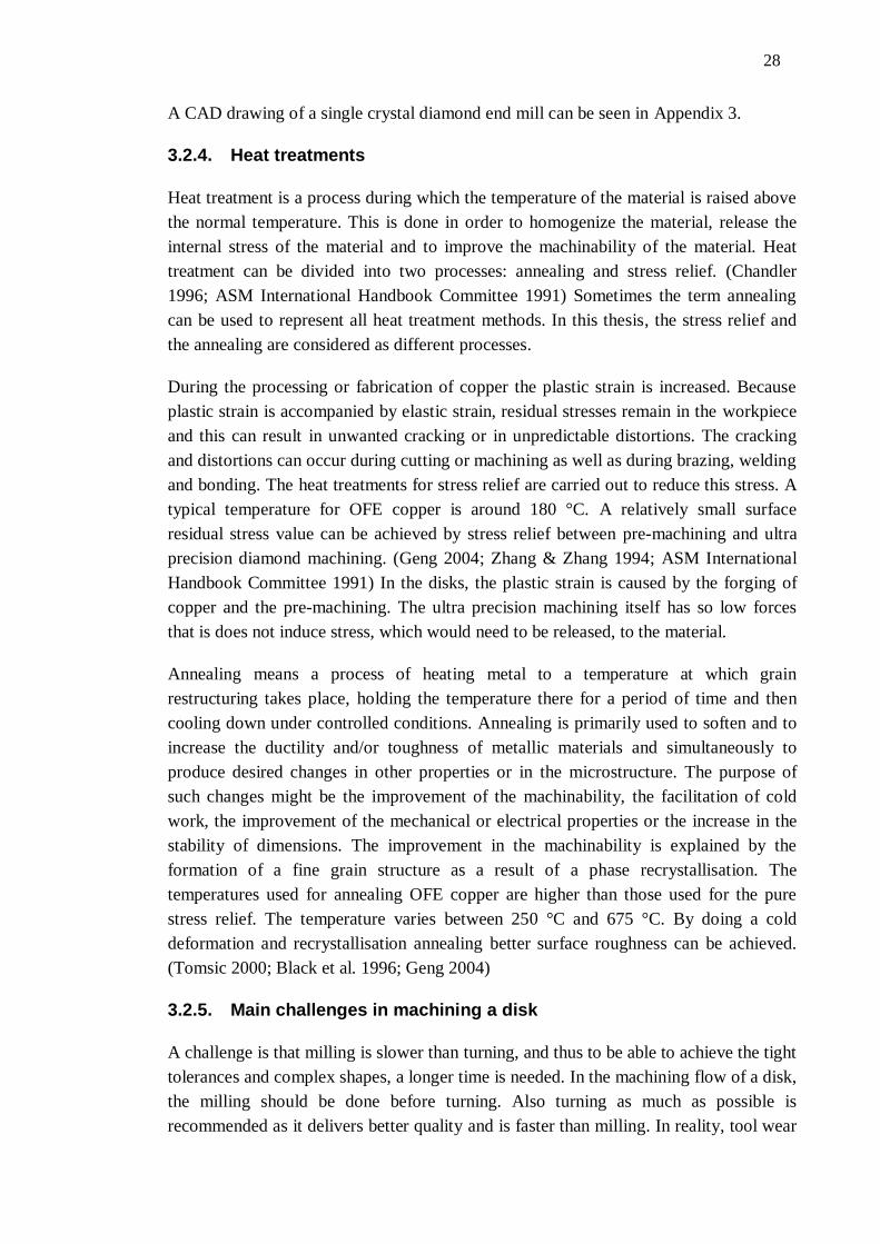
3.2.5. Main challenges in machining a disk
A challenge is that milling is slower than turning, and thus to be able to achieve the tight
tolerances and complex shapes, a longer time is needed. In the machining flow of a disk,
the milling should be done before turning. Also turning as much as possible is
recommended as it delivers better quality and is faster than milling. In reality, tool wear
29
and minor changes in atmosphere temperature and humidity can cause dramatic changes
in the quality. That is why a controlled environment is needed.
Changing from turning to milling can cause problems in some setups. If the machine
does not include both turning and milling in the same setup, the workpiece has to be
detached and attached between working phases. This can cause visible clamping
damage as well as geometrical errors. In Figure 3.14, there is a visible step between
turning and milling caused by the loss of the reference point while unclamping and
reclamping the workpiece. This is a result of milling the workpiece first and then trying
to attach the workpiece again in the correct place in the turning setup. As a result, the
reference point of the turning setup is not the same as it was with the milling setup.
Figure 3.14. SEM micrograph of a copper disk with both milling and turning marks
visible (Micrograph by M. Aicheler, courtesy of CERN).
In the disk drawings (e.g. Figure 2.7), the corners inside the pockets have a radius of 0.5
mm. This is due to the fact that the pockets are to be milled with a ball end mill, which
has a certain radius. So the radius of the corner has to be greater or equal to the radius of
the ball end mill used for ultra precision milling. Going to smaller radius i.e. closer to
right angle, a smaller cutting tool would be needed and the smaller radius of the cutting
tool would increase the machining time and add unnecessary setup time due to the tool
change.
Milling
Turning
30
4. GEOMETRICAL MEASUREMENTS
Geometrical measurements are done in order verify the given tolerances. Measurements
are done in a purpose build laboratory and with either contact or non-contact
measurement devices. The measured parameters of the disk are the surface roughness,
shape accuracy and flatness. All of these are measured in various parts of the disk.
4.1. Measurement techniques
Two basic types of measurement machines exist: contact and non-contact. A contact
measurement system can be used to measure geometrical quantities of a workpiece
(Weckenmann et al. 2004). Optical non-contact measurement machines are usually used
to measure surface roughness and it is expected that they could be used also as high
precision coordinate measuring machines (CMM) in the future (Thomas 1999; Elepano
2010).
It is also good to distinguish two types of measurement systems that are used. First type
of system is for coordinate metrology and the second type for profile metrology. The
machines have developed so that both types usually have a reference axis and a data
processing computer. Therefore both can be called a coordinate measuring machine.
(Takamasu et al. 1996)
4.1.1. Contact measurement
A basic contact measurement system is based on a stylus, whose movements are
amplified. In contact measurement, a workpiece is set in the range of a probing system,
and then the probe is brought in contact with the workpiece. After that the probe is slid
on the surface of the workpiece and the output of the system is measured. If a drive and
a position measurement system are added to the existing system, a CMM system is
achieved. (Weckenmann et al. 2004) Otherwise the system just measures the surface
profile. Figure 4.1 describes the basic principle of a contact measurement system for the
calculation of surface roughness.
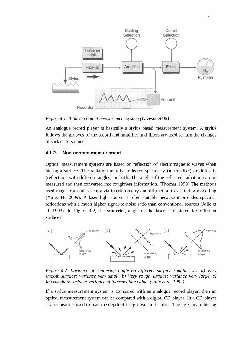
31
Figure 4.1. A basic contact measurement system (Grzesik 2008).
An analogue record player is basically a stylus based measurement system. A stylus
follows the grooves of the record and amplifier and filters are used to turn the changes
of surface to sounds.
4.1.2. Non-contact measurement
Optical measurement systems are based on reflection of electromagnetic waves when
hitting a surface. The radiation may be reflected specularly (mirror-like) or diffusely
(reflections with different angles) or both. The angle of the reflected radiation can be
measured and then converted into roughness information. (Thomas 1999) The methods
used range from microscopy via interferometry and diffraction to scattering modelling
(Xu & Hu 2009). A laser light source is often suitable because it provides specular
reflections with a much higher signal-to-noise ratio than conventional sources (Jolic et
al. 1993). In Figure 4.2, the scattering angle of the laser is depicted for different
surfaces.
Figure 4.2. Variance of scattering angle on different surface roughnesses. a) Very
smooth surface; variance very small. b) Very rough surface; variance very large. c)
Intermediate surface; variance of intermediate value. (Jolic et al. 1994)
If a stylus measurement system is compared with an analogue record player, then an
optical measurement system can be compared with a digital CD-player. In a CD-player
a laser beam is used to read the depth of the grooves in the disc. The laser beam hitting
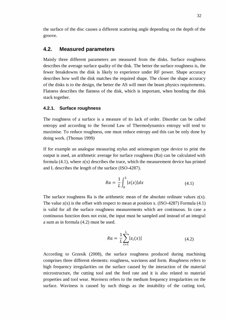
32
the surface of the disc causes a different scattering angle depending on the depth of the
groove.
4.2. Measured parameters
Mainly three different parameters are measured from the disks. Surface roughness
describes the average surface quality of the disk. The better the surface roughness is, the
fewer breakdowns the disk is likely to experience under RF power. Shape accuracy
describes how well the disk matches the required shape. The closer the shape accuracy
of the disks is to the design, the better the AS will meet the beam physics requirements.
Flatness describes the flatness of the disk, which is important, when bonding the disk
stack together.
4.2.1. Surface roughness
The roughness of a surface is a measure of its lack of order. Disorder can be called
entropy and according to the Second Law of Thermodynamics entropy will tend to
maximise. To reduce roughness, one must reduce entropy and this can be only done by
doing work. (Thomas 1999)
If for example an analogue measuring stylus and seismogram type device to print the
output is used, an arithmetic average for surface roughness (Ra) can be calculated with
formula (4.1), where z(x) describes the trace, which the measurement device has printed
and L describes the length of the surface (ISO-4287).
(4.1)
The surface roughness Ra is the arithmetic mean of the absolute ordinate values z(x).
The value z(x) is the offset with respect to mean at position x. (ISO-4287) Formula (4.1)
is valid for all the surface roughness measurements which are continuous. In case a
continuous function does not exist, the input must be sampled and instead of an integral
a sum as in formula (4.2) must be used.
(4.2)
According to Grzesik (2008), the surface roughness produced during machining
comprises three different elements: roughness, waviness and form. Roughness refers to
high frequency irregularities on the surface caused by the interaction of the material
microstructure, the cutting tool and the feed rate and it is also related to material
properties and tool wear. Waviness refers to the medium frequency irregularities on the
surface. Waviness is caused by such things as the instability of the cutting tool,
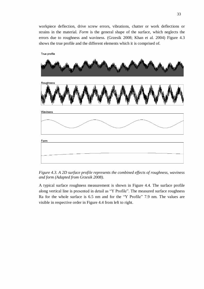
33
workpiece deflection, drive screw errors, vibrations, chatter or work deflections or
strains in the material. Form is the general shape of the surface, which neglects the
errors due to roughness and waviness. (Grzesik 2008; Khan et al. 2004) Figure 4.3
shows the true profile and the different elements which it is comprised of.
Figure 4.3. A 2D surface profile represents the combined effects of roughness, waviness
and form (Adapted from Grzesik 2008).
A typical surface roughness measurement is shown in Figure 4.4. The surface profile
along vertical line is presented in detail as “Y Profile”. The measured surface roughness
Ra for the whole surface is 6.5 nm and for the “Y Profile” 7.9 nm. The values are
visible in respective order in Figure 4.4 from left to right.
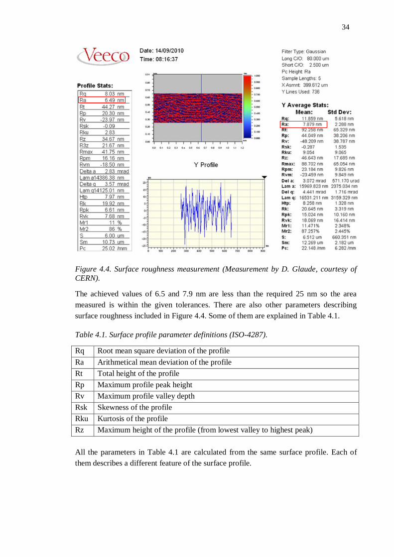
34
Figure 4.4. Surface roughness measurement (Measurement by D. Glaude, courtesy of
CERN).
The achieved values of 6.5 and 7.9 nm are less than the required 25 nm so the area
measured is within the given tolerances. There are also other parameters describing
surface roughness included in Figure 4.4. Some of them are explained in Table 4.1.
Table 4.1. Surface profile parameter definitions (ISO-4287).
Rq Root mean square deviation of the profile
Ra Arithmetical mean deviation of the profile
Rt Total height of the profile
Rp Maximum profile peak height
Rv Maximum profile valley depth
Rsk Skewness of the profile
Rku Kurtosis of the profile
Rz Maximum height of the profile (from lowest valley to highest peak)
All the parameters in Table 4.1 are calculated from the same surface profile. Each of
them describes a different feature of the surface profile.
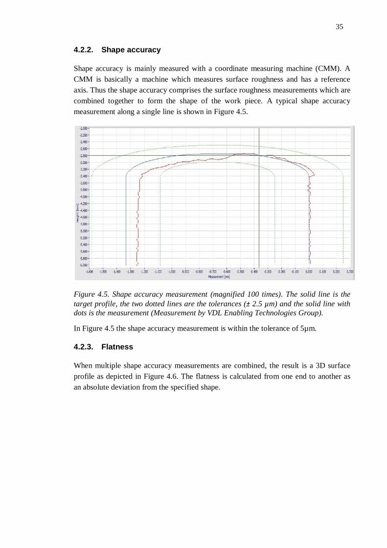
35
4.2.2. Shape accuracy
Shape accuracy is mainly measured with a coordinate measuring machine (CMM). A
CMM is basically a machine which measures surface roughness and has a reference
axis. Thus the shape accuracy comprises the surface roughness measurements which are
combined together to form the shape of the work piece. A typical shape accuracy
measurement along a single line is shown in Figure 4.5.
Figure 4.5. Shape accuracy measurement (magnified 100 times). The solid line is the
target profile, the two dotted lines are the tolerances (± 2.5 µm) and the solid line with
dots is the measurement (Measurement by VDL Enabling Technologies Group).
In Figure 4.5 the shape accuracy measurement is within the tolerance of 5µm.
4.2.3. Flatness
When multiple shape accuracy measurements are combined, the result is a 3D surface
profile as depicted in Figure 4.6. The flatness is calculated from one end to another as
an absolute deviation from the specified shape.
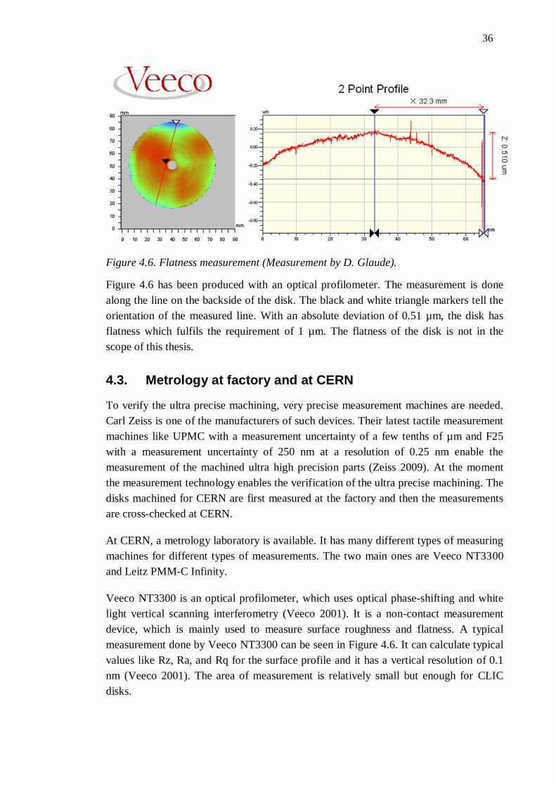
36
Figure 4.6. Flatness measurement (Measurement by D. Glaude).
Figure 4.6 has been produced with an optical profilometer. The measurement is done
along the line on the backside of the disk. The black and white triangle markers tell the
orientation of the measured line. With an absolute deviation of 0.51 µm, the disk has
flatness which fulfils the requirement of 1 µm. The flatness of the disk is not in the
scope of this thesis.
4.3. Metrology at factory and at CERN
To verify the ultra precise machining, very precise measurement machines are needed.
Carl Zeiss is one of the manufacturers of such devices. Their latest tactile measurement
machines like UPMC with a measurement uncertainty of a few tenths of µm and F25
with a measurement uncertainty of 250 nm at a resolution of 0.25 nm enable the
measurement of the machined ultra high precision parts (Zeiss 2009). At the moment
the measurement technology enables the verification of the ultra precise machining. The
disks machined for CERN are first measured at the factory and then the measurements
are cross-checked at CERN.
At CERN, a metrology laboratory is available. It has many different types of measuring
machines for different types of measurements. The two main ones are Veeco NT3300
and Leitz PMM-C Infinity.
Veeco NT3300 is an optical profilometer, which uses optical phase-shifting and white
light vertical scanning interferometry (Veeco 2001). It is a non-contact measurement
device, which is mainly used to measure surface roughness and flatness. A typical
measurement done by Veeco NT3300 can be seen in Figure 4.6. It can calculate typical
values like Rz, Ra, and Rq for the surface profile and it has a vertical resolution of 0.1
nm (Veeco 2001). The area of measurement is relatively small but enough for CLIC
disks.

37
Leitz Infinity is a contact measurement device which uses a probe head to probe the
measured workpiece. It is mainly used to measure shape accuracy. Leitz Infinity
weights 7.5 tons and it sits on three vibration dampers (CERN Bulletin 2011). The
maximum measurement area for Leitz is 1200 x 1000 x 700 mm, so it can be used to
measure large pieces. It has an accuracy of ±0.3 μm over 1 meter length (Leitz 2011).
The standard probing force is between 0.02-0.16 N, which can cause some visible
damage on soft surfaces like copper. A modified probing head with lower probing force
(0.005-0.10 N) prevents this from happening. When the probing head comes in touch
with the surface, it sends the precise coordinates of its point of contact via optical rulers
(CERN Bulletin 2011). Leitz Infinity is located in its own room inside a bigger room in
a stable environment. The reference temperature is 20 °C and the allowed gradients for
the room are: 0.2 °C / hour, 0.4 °C / day and 0.1 °C / meter. The temperature control is
required to keep the whole workpiece and the measurement device under monitored
conditions. (Cherif 2011)
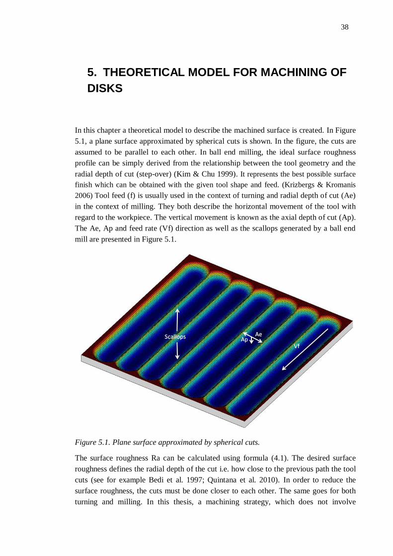
38
5. THEORETICAL MODEL FOR MACHINING OF
DISKS
In this chapter a theoretical model to describe the machined surface is created. In Figure
5.1, a plane surface approximated by spherical cuts is shown. In the figure, the cuts are
assumed to be parallel to each other. In ball end milling, the ideal surface roughness
profile can be simply derived from the relationship between the tool geometry and the
radial depth of cut (step-over) (Kim & Chu 1999). It represents the best possible surface
finish which can be obtained with the given tool shape and feed. (Krizbergs & Kromanis
2006) Tool feed (f) is usually used in the context of turning and radial depth of cut (Ae)
in the context of milling. They both describe the horizontal movement of the tool with
regard to the workpiece. The vertical movement is known as the axial depth of cut (Ap).
The Ae, Ap and feed rate (Vf) direction as well as the scallops generated by a ball end
mill are presented in Figure 5.1.
Figure 5.1. Plane surface approximated by spherical cuts.
The surface roughness Ra can be calculated using formula (4.1). The desired surface
roughness defines the radial depth of the cut i.e. how close to the previous path the tool
cuts (see for example Bedi et al. 1997; Quintana et al. 2010). In order to reduce the
surface roughness, the cuts must be done closer to each other. The same goes for both
turning and milling. In this thesis, a machining strategy, which does not involve
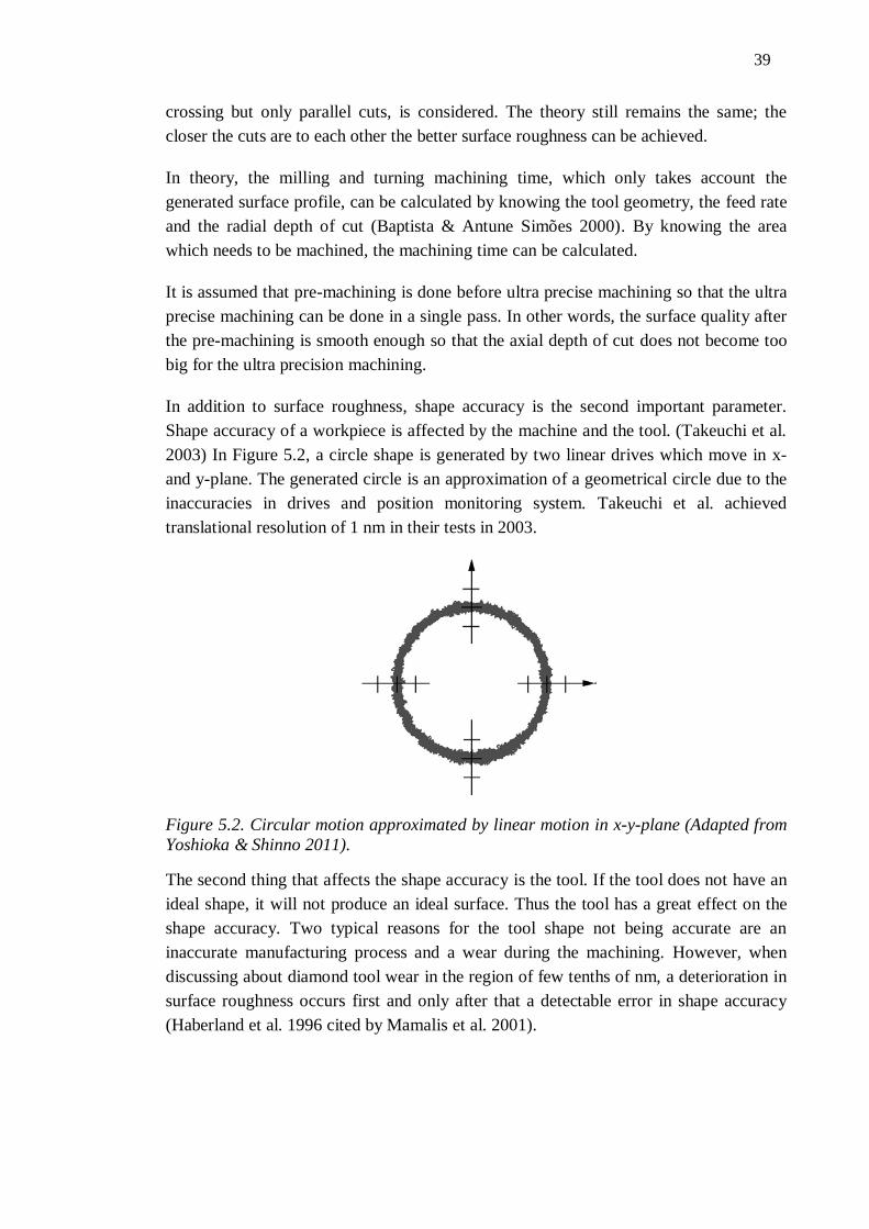
39
crossing but only parallel cuts, is considered. The theory still remains the same; the
closer the cuts are to each other the better surface roughness can be achieved.
In theory, the milling and turning machining time, which only takes account the
generated surface profile, can be calculated by knowing the tool geometry, the feed rate
and the radial depth of cut (Baptista & Antune Simões 2000). By knowing the area
which needs to be machined, the machining time can be calculated.
It is assumed that pre-machining is done before ultra precise machining so that the ultra
precise machining can be done in a single pass. In other words, the surface quality after
the pre-machining is smooth enough so that the axial depth of cut does not become too
big for the ultra precision machining.
In addition to surface roughness, shape accuracy is the second important parameter.
Shape accuracy of a workpiece is affected by the machine and the tool. (Takeuchi et al.
2003) In Figure 5.2, a circle shape is generated by two linear drives which move in x-
and y-plane. The generated circle is an approximation of a geometrical circle due to the
inaccuracies in drives and position monitoring system. Takeuchi et al. achieved
translational resolution of 1 nm in their tests in 2003.
Figure 5.2. Circular motion approximated by linear motion in x-y-plane (Adapted from
Yoshioka & Shinno 2011).
The second thing that affects the shape accuracy is the tool. If the tool does not have an
ideal shape, it will not produce an ideal surface. Thus the tool has a great effect on the
shape accuracy. Two typical reasons for the tool shape not being accurate are an
inaccurate manufacturing process and a wear during the machining. However, when
discussing about diamond tool wear in the region of few tenths of nm, a deterioration in
surface roughness occurs first and only after that a detectable error in shape accuracy
(Haberland et al. 1996 cited by Mamalis et al. 2001).
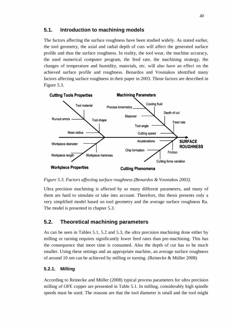
40
5.1. Introduction to machining models
The factors affecting the surface roughness have been studied widely. As stated earlier,
the tool geometry, the axial and radial depth of cuts will affect the generated surface
profile and thus the surface roughness. In reality, the tool wear, the machine accuracy,
the used numerical computer program, the feed rate, the machining strategy, the
changes of temperature and humidity, materials, etc. will also have an effect on the
achieved surface profile and roughness. Benardos and Vosniakos identified many
factors affecting surface roughness in their paper in 2003. Those factors are described in
Figure 5.3.
Figure 5.3. Factors affecting surface roughness (Benardos & Vosniakos 2003).
Ultra precision machining is affected by so many different parameters, and many of
them are hard to simulate or take into account. Therefore, this thesis presents only a
very simplified model based on tool geometry and the average surface roughness Ra.
The model is presented in chapter 5.3.
5.2. Theoretical machining parameters
As can be seen in Tables 5.1, 5.2 and 5.3, the ultra precision machining done either by
milling or turning requires significantly lower feed rates than pre-machining. This has
the consequence that more time is consumed. Also the depth of cut has to be much
smaller. Using these settings and an appropriate machine, an average surface roughness
of around 10 nm can be achieved by milling or turning. (Reinecke & Müller 2008)
5.2.1. Milling
According to Reinecke and Müller (2008) typical process parameters for ultra precision
milling of OFE copper are presented in Table 5.1. In milling, considerably high spindle
speeds must be used. The reasons are that the tool diameter is small and the tool might
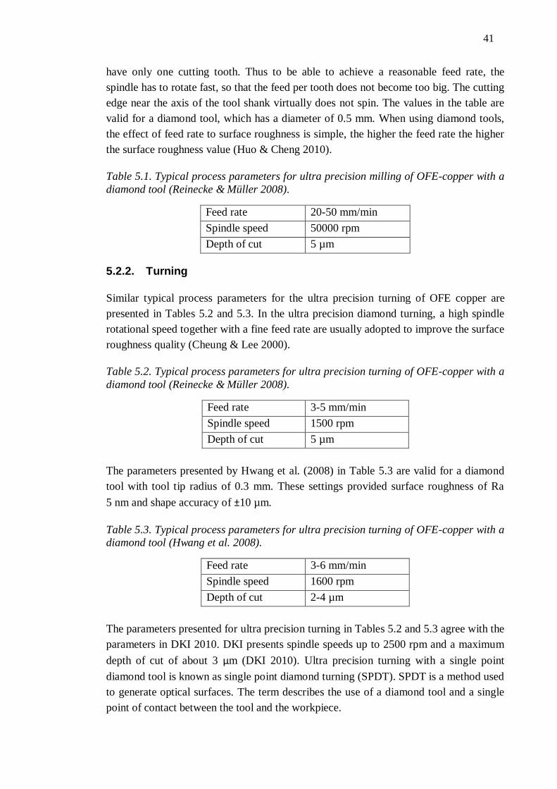
41
have only one cutting tooth. Thus to be able to achieve a reasonable feed rate, the
spindle has to rotate fast, so that the feed per tooth does not become too big. The cutting
edge near the axis of the tool shank virtually does not spin. The values in the table are
valid for a diamond tool, which has a diameter of 0.5 mm. When using diamond tools,
the effect of feed rate to surface roughness is simple, the higher the feed rate the higher
the surface roughness value (Huo & Cheng 2010).
Table 5.1. Typical process parameters for ultra precision milling of OFE-copper with a
diamond tool (Reinecke & Müller 2008).
Feed rate 20-50 mm/min
Spindle speed 50000 rpm
Depth of cut 5 µm
5.2.2. Turning
Similar typical process parameters for the ultra precision turning of OFE copper are
presented in Tables 5.2 and 5.3. In the ultra precision diamond turning, a high spindle
rotational speed together with a fine feed rate are usually adopted to improve the surface
roughness quality (Cheung & Lee 2000).
Table 5.2. Typical process parameters for ultra precision turning of OFE-copper with a
diamond tool (Reinecke & Müller 2008).
Feed rate 3-5 mm/min
Spindle speed 1500 rpm
Depth of cut 5 µm
The parameters presented by Hwang et al. (2008) in Table 5.3 are valid for a diamond
tool with tool tip radius of 0.3 mm. These settings provided surface roughness of Ra
5 nm and shape accuracy of ±10 µm.
Table 5.3. Typical process parameters for ultra precision turning of OFE-copper with a
diamond tool (Hwang et al. 2008).
Feed rate 3-6 mm/min
Spindle speed 1600 rpm
Depth of cut 2-4 µm
The parameters presented for ultra precision turning in Tables 5.2 and 5.3 agree with the
parameters in DKI 2010. DKI presents spindle speeds up to 2500 rpm and a maximum
depth of cut of about 3 µm (DKI 2010). Ultra precision turning with a single point
diamond tool is known as single point diamond turning (SPDT). SPDT is a method used
to generate optical surfaces. The term describes the use of a diamond tool and a single
point of contact between the tool and the workpiece.
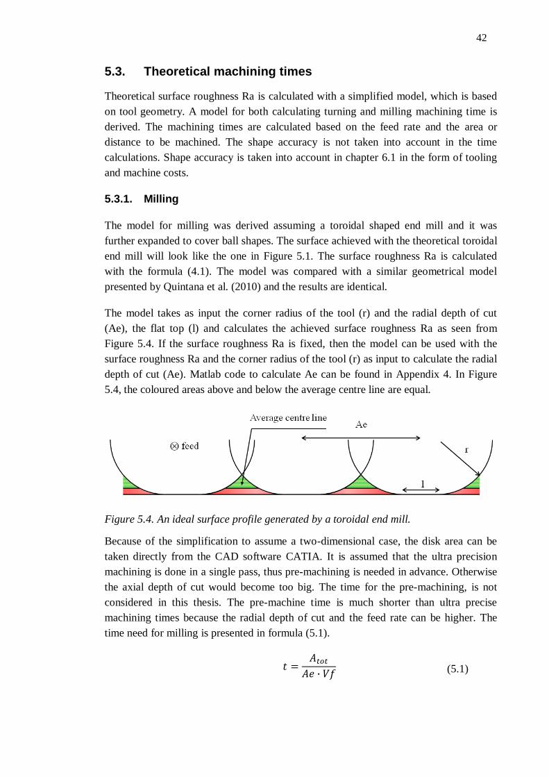
42
5.3. Theoretical machining times
Theoretical surface roughness Ra is calculated with a simplified model, which is based
on tool geometry. A model for both calculating turning and milling machining time is
derived. The machining times are calculated based on the feed rate and the area or
distance to be machined. The shape accuracy is not taken into account in the time
calculations. Shape accuracy is taken into account in chapter 6.1 in the form of tooling
and machine costs.
5.3.1. Milling
The model for milling was derived assuming a toroidal shaped end mill and it was
further expanded to cover ball shapes. The surface achieved with the theoretical toroidal
end mill will look like the one in Figure 5.1. The surface roughness Ra is calculated
with the formula (4.1). The model was compared with a similar geometrical model
presented by Quintana et al. (2010) and the results are identical.
The model takes as input the corner radius of the tool (r) and the radial depth of cut
(Ae), the flat top (l) and calculates the achieved surface roughness Ra as seen from
Figure 5.4. If the surface roughness Ra is fixed, then the model can be used with the
surface roughness Ra and the corner radius of the tool (r) as input to calculate the radial
depth of cut (Ae). Matlab code to calculate Ae can be found in Appendix 4. In Figure
5.4, the coloured areas above and below the average centre line are equal.
Figure 5.4. An ideal surface profile generated by a toroidal end mill.
Because of the simplification to assume a two-dimensional case, the disk area can be
taken directly from the CAD software CATIA. It is assumed that the ultra precision
machining is done in a single pass, thus pre-machining is needed in advance. Otherwise
the axial depth of cut would become too big. The time for the pre-machining, is not
considered in this thesis. The pre-machine time is much shorter than ultra precise
machining times because the radial depth of cut and the feed rate can be higher. The
time need for milling is presented in formula (5.1).
(5.1)
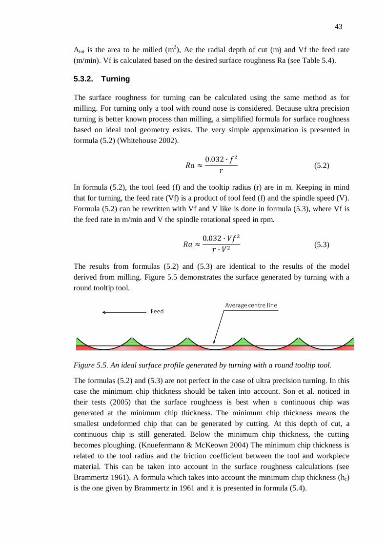
43
Atot is the area to be milled (m2), Ae the radial depth of cut (m) and Vf the feed rate
(m/min). Vf is calculated based on the desired surface roughness Ra (see Table 5.4).
5.3.2. Turning
The surface roughness for turning can be calculated using the same method as for
milling. For turning only a tool with round nose is considered. Because ultra precision
turning is better known process than milling, a simplified formula for surface roughness
based on ideal tool geometry exists. The very simple approximation is presented in
formula (5.2) (Whitehouse 2002).
(5.2)
In formula (5.2), the tool feed (f) and the tooltip radius (r) are in m. Keeping in mind
that for turning, the feed rate (Vf) is a product of tool feed (f) and the spindle speed (V).
Formula (5.2) can be rewritten with Vf and V like is done in formula (5.3), where Vf is
the feed rate in m/min and V the spindle rotational speed in rpm.
(5.3)
The results from formulas (5.2) and (5.3) are identical to the results of the model
derived from milling. Figure 5.5 demonstrates the surface generated by turning with a
round tooltip tool.
Figure 5.5. An ideal surface profile generated by turning with a round tooltip tool.
The formulas (5.2) and (5.3) are not perfect in the case of ultra precision turning. In this
case the minimum chip thickness should be taken into account. Son et al. noticed in
their tests (2005) that the surface roughness is best when a continuous chip was
generated at the minimum chip thickness. The minimum chip thickness means the
smallest undeformed chip that can be generated by cutting. At this depth of cut, a
continuous chip is still generated. Below the minimum chip thickness, the cutting
becomes ploughing. (Knuefermann & McKeown 2004) The minimum chip thickness is
related to the tool radius and the friction coefficient between the tool and workpiece
material. This can be taken into account in the surface roughness calculations (see
Brammertz 1961). A formula which takes into account the minimum chip thickness (hc)
is the one given by Brammertz in 1961 and it is presented in formula (5.4).
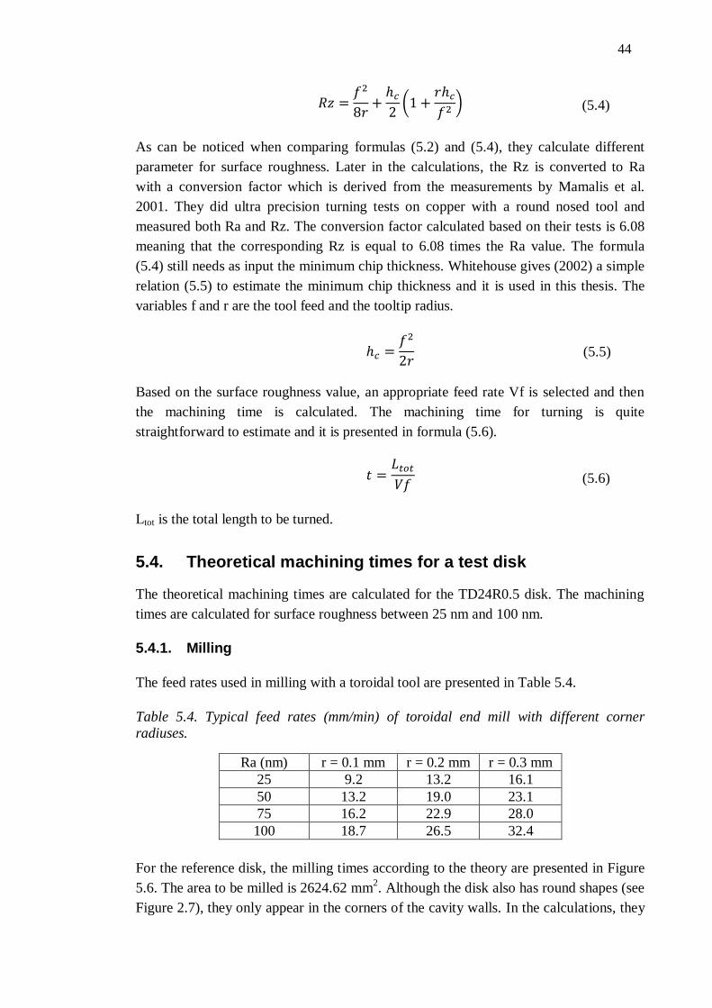
44
(5.4)
As can be noticed when comparing formulas (5.2) and (5.4), they calculate different
parameter for surface roughness. Later in the calculations, the Rz is converted to Ra
with a conversion factor which is derived from the measurements by Mamalis et al.
2001. They did ultra precision turning tests on copper with a round nosed tool and
measured both Ra and Rz. The conversion factor calculated based on their tests is 6.08
meaning that the corresponding Rz is equal to 6.08 times the Ra value. The formula
(5.4) still needs as input the minimum chip thickness. Whitehouse gives (2002) a simple
relation (5.5) to estimate the minimum chip thickness and it is used in this thesis. The
variables f and r are the tool feed and the tooltip radius.
(5.5)
Based on the surface roughness value, an appropriate feed rate Vf is selected and then
the machining time is calculated. The machining time for turning is quite
straightforward to estimate and it is presented in formula (5.6).
(5.6)
Ltot is the total length to be turned.
5.4. Theoretical machining times for a test disk
The theoretical machining times are calculated for the TD24R0.5 disk. The machining
times are calculated for surface roughness between 25 nm and 100 nm.
5.4.1. Milling
The feed rates used in milling with a toroidal tool are presented in Table 5.4.
Table 5.4. Typical feed rates (mm/min) of toroidal end mill with different corner
radiuses.
Ra (nm) r = 0.1 mm r = 0.2 mm r = 0.3 mm
25 9.2 13.2 16.1
50 13.2 19.0 23.1
75 16.2 22.9 28.0
100 18.7 26.5 32.4
For the reference disk, the milling times according to the theory are presented in Figure
5.6. The area to be milled is 2624.62 mm2. Although the disk also has round shapes (see
Figure 2.7), they only appear in the corners of the cavity walls. In the calculations, they
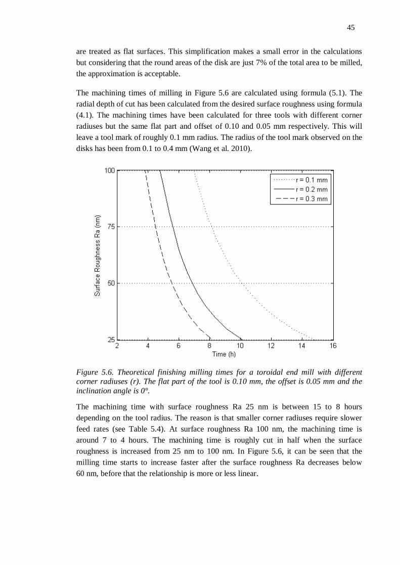
45
are treated as flat surfaces. This simplification makes a small error in the calculations
but considering that the round areas of the disk are just 7% of the total area to be milled,
the approximation is acceptable.
The machining times of milling in Figure 5.6 are calculated using formula (5.1). The
radial depth of cut has been calculated from the desired surface roughness using formula
(4.1). The machining times have been calculated for three tools with different corner
radiuses but the same flat part and offset of 0.10 and 0.05 mm respectively. This will
leave a tool mark of roughly 0.1 mm radius. The radius of the tool mark observed on the
disks has been from 0.1 to 0.4 mm (Wang et al. 2010).
Figure 5.6. Theoretical finishing milling times for a toroidal end mill with different
corner radiuses (r). The flat part of the tool is 0.10 mm, the offset is 0.05 mm and the
inclination angle is 0°.
The machining time with surface roughness Ra 25 nm is between 15 to 8 hours
depending on the tool radius. The reason is that smaller corner radiuses require slower
feed rates (see Table 5.4). At surface roughness Ra 100 nm, the machining time is
around 7 to 4 hours. The machining time is roughly cut in half when the surface
roughness is increased from 25 nm to 100 nm. In Figure 5.6, it can be seen that the
milling time starts to increase faster after the surface roughness Ra decreases below
60 nm, before that the relationship is more or less linear.
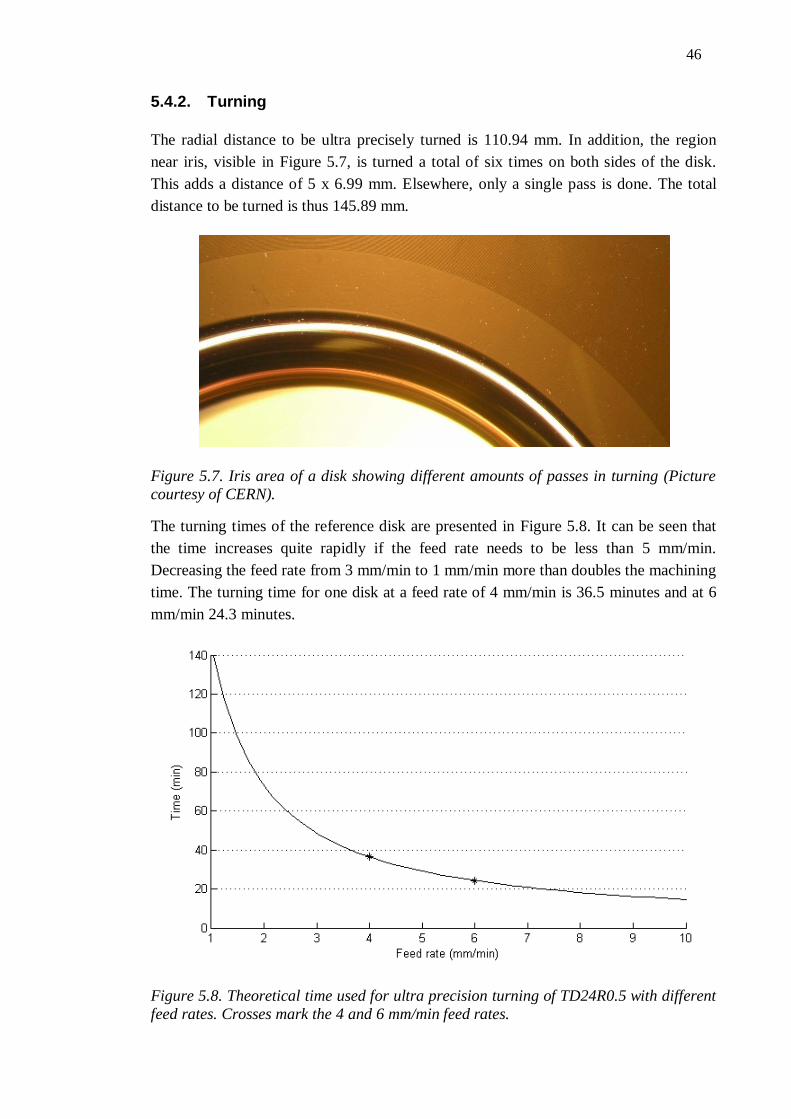
46
5.4.2. Turning
The radial distance to be ultra precisely turned is 110.94 mm. In addition, the region
near iris, visible in Figure 5.7, is turned a total of six times on both sides of the disk.
This adds a distance of 5 x 6.99 mm. Elsewhere, only a single pass is done. The total
distance to be turned is thus 145.89 mm.
Figure 5.7. Iris area of a disk showing different amounts of passes in turning (Picture
courtesy of CERN).
The turning times of the reference disk are presented in Figure 5.8. It can be seen that
the time increases quite rapidly if the feed rate needs to be less than 5 mm/min.
Decreasing the feed rate from 3 mm/min to 1 mm/min more than doubles the machining
time. The turning time for one disk at a feed rate of 4 mm/min is 36.5 minutes and at 6
mm/min 24.3 minutes.
Figure 5.8. Theoretical time used for ultra precision turning of TD24R0.5 with different
feed rates. Crosses mark the 4 and 6 mm/min feed rates.
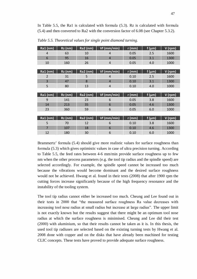
47
In Table 5.5, the Ra1 is calculated with formula (5.3). Rz is calculated with formula
(5.4) and then converted to Ra2 with the conversion factor of 6.08 (see Chapter 5.3.2).
Table 5.5. Theoretical values for single point diamond turning.
Ra1 (nm) Rz (nm) Ra2 (nm) Vf (mm/min) r (mm) f (µm) V (rpm)
4 63 10 4 0.05 2.5 1600
6 95 16 4 0.05 3.1 1300
10 160 26 4 0.05 4.0 1000
Ra1 (nm) Rz (nm) Ra2 (nm) Vf (mm/min) r (mm) f (µm) V (rpm)
2 31 5 4 0.10 2.5 1600
3 47 8 4 0.10 3.1 1300
5 80 13 4 0.10 4.0 1000
Ra1 (nm) Rz (nm) Ra2 (nm) Vf (mm/min) r (mm) f (µm) V (rpm)
9 141 23 6 0.05 3.8 1600
14 213 35 6 0.05 4.6 1300
23 360 59 6 0.05 6.0 1000
Ra1 (nm) Rz (nm) Ra2 (nm) Vf (mm/min) r (mm) f (µm) V (rpm)
5 70 12 6 0.10 3.8 1600
7 107 18 6 0.10 4.6 1300
12 180 30 6 0.10 6.0 1000
Brammertz’ formula (5.4) should give more realistic values for surface roughness than
formula (5.3) which gives optimistic values in case of ultra precision turning. According
to Table 5.5, the feed rates between 4-6 mm/min provide surface roughness up to few
nm when the other process parameters (e.g. the tool tip radius and the spindle speed) are
selected accordingly. For example, the spindle speed cannot be increased too much
because the vibrations would become dominant and the desired surface roughness
would not be achieved. Hwang et al. found in their tests (2008) that after 1900 rpm the
cutting forces increase significantly because of the high frequency resonance and the
instability of the tooling system.
The tool tip radius cannot either be increased too much. Cheung and Lee found out in
their tests in 2000 that “the measured surface roughness Ra value decreases with
increasing tool nose radius at small radius but increase at large radius”. The upper limit
is not exactly known but the results suggest that there might be an optimum tool nose
radius at which the surface roughness is minimised. Cheung and Lee did their test
(2000) with aluminium, so that their results cannot be taken as it is. In this thesis, the
used tool tip radiuses are selected based on the existing turning tests by Hwang et al.
2008 done with copper and on the disks that have already been machined for testing
CLIC concepts. These tests have proved to provide adequate surface roughness.
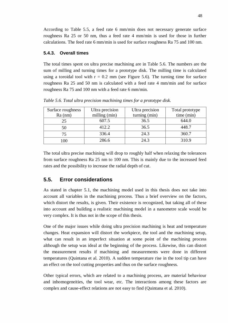
48
According to Table 5.5, a feed rate 6 mm/min does not necessary generate surface
roughness Ra 25 or 50 nm, thus a feed rate 4 mm/min is used for those in further
calculations. The feed rate 6 mm/min is used for surface roughness Ra 75 and 100 nm.
5.4.3. Overall times
The total times spent on ultra precise machining are in Table 5.6. The numbers are the
sum of milling and turning times for a prototype disk. The milling time is calculated
using a toroidal tool with r = 0.2 mm (see Figure 5.6). The turning time for surface
roughness Ra 25 and 50 nm is calculated with a feed rate 4 mm/min and for surface
roughness Ra 75 and 100 nm with a feed rate 6 mm/min.
Table 5.6. Total ultra precision machining times for a prototype disk.
Surface roughness
Ra (nm)
Ultra precision
milling (min)
Ultra precision
turning (min)
Total prototype
time (min)
25 607.5 36.5 644.0
50 412.2 36.5 448.7
75 336.4 24.3 360.7
100 286.6 24.3 310.9
The total ultra precise machining will drop to roughly half when relaxing the tolerances
from surface roughness Ra 25 nm to 100 nm. This is mainly due to the increased feed
rates and the possibility to increase the radial depth of cut.
5.5. Error considerations
As stated in chapter 5.1, the machining model used in this thesis does not take into
account all variables in the machining process. Thus a brief overview on the factors,
which distort the results, is given. Their existence is recognized, but taking all of these
into account and building a realistic machining model in a nanometre scale would be
very complex. It is thus not in the scope of this thesis.
One of the major issues while doing ultra precision machining is heat and temperature
changes. Heat expansion will distort the workpiece, the tool and the machining setup,
what can result in an imperfect situation at some point of the machining process
although the setup was ideal at the beginning of the process. Likewise, this can distort
the measurement results if machining and measurements were done in different
temperatures (Quintana et al. 2010). A sudden temperature rise in the tool tip can have
an effect on the tool cutting properties and thus on the surface roughness.
Other typical errors, which are related to a machining process, are material behaviour
and inhomogeneities, the tool wear, etc. The interactions among these factors are
complex and cause-effect relations are not easy to find (Quintana et al. 2010).
49
Especially in milling, it has to be taken into account that the tool has to cut also other
than perpendicular surfaces. This is why a 5-axis milling machine is needed. Increasing
the number of axes increases the number of error sources. The shapes generated by
milling are usually more complex than the ones generated by turning, which makes it
more challenging to the machine and the process and thus more prone to errors.
The model based on an ideal surface roughness profile is not perfect as Cheung & Lee
(2000) state. For turning, the arithmetic roughness values determined from the ideal
surface roughness profile make a quite good prediction under low spindle speed and
large feed rate conditions. However, the discrepancy between the two increases with
increasing the spindle rotational speed and decreasing the feed rate. (Cheung & Lee
2000)
One error source, which is not taken into account but can affect the results, is the tool
vibration. While cutting, the tool vibrates mostly up and down altering the depth of cut.
This vibration can be calculated by knowing the frequency whereby system is vibrating
(Cheung & Lee 2000). The surface profile can be simulated with the known frequency
and other process parameters (Cheung & Lee 2000). The problem is that if the
machinist aims to cut at the minimum chip thickness, the vibrations might alter the
intended depth of cut. If the depth of cut changes uncontrollably during the cutting
process, it might go below or above the minimum chip thickness, which causes a fast
deterioration of the surface roughness.
50
6. COST ESTIMATE METHOD AND
PARAMETERS
The cost estimate for the production of CLIC AS is otherwise similar than in the
previous study (Uusimäki & Saifoulina 2010) except now the machining time of a disk
is based on the previous chapter and so-called learning curves. A noticeable thing in this
study, and also in the one prepared by Uusimäki & Saifoulina (2010), is that the cost
estimate is calculated assuming multiple separate production lines.
6.1. Cost method
The cost estimate method in this thesis is explained in this chapter. The end result will
be the cost estimate of the AS made out of disks for CLIC at 3 TeV. In this study, the
needed number of machines and operators will be derived from the time needed for
machining. When both the surface roughness Ra and shape accuracy tolerances are
relaxed, also the tooling and machinery costs are assumed to decrease. Some costs are
not dependent on surface roughness or shape accuracy. For these costs, the same values
as in the previous study drafted by Uusimäki & Saifoulina (2010) will be used.
The cost function takes as input the machining times for different phases of machining,
e.g. pre-machining, precise machining and ultra precise machining. Although in this
thesis, the pre-machining and precise machining times are constant. The model in Excel
is used to calculate the needed number of machines and workers. Five shifts are
considered. Some additional parts like cooling circuits, vacuum manifolds and damping
materials are also considered. Their price is constant. Buildings, electricity, clean room
and interest costs are all taken into account. The cost function includes all the
machining steps as well as the entire assembly procedure to fabricate an AS. A failure
rate was not considered in the calculations for this thesis. The costs were calculated
assuming that the production is divided between two, three or four production lines.
This is done to reduce the risk of having only a single supplier and also to create
competition among the suppliers. The number of production lines will have an effect on
the learning curves and on the fixed costs.
6.2. Learning curves
The concept of learning curves was first presented by Wright in 1936. The hypothesis is
that in repetitive production the time will decrease a constant percentage each time the
production quantity is doubled. Thus the average cost of a product can be calculated if
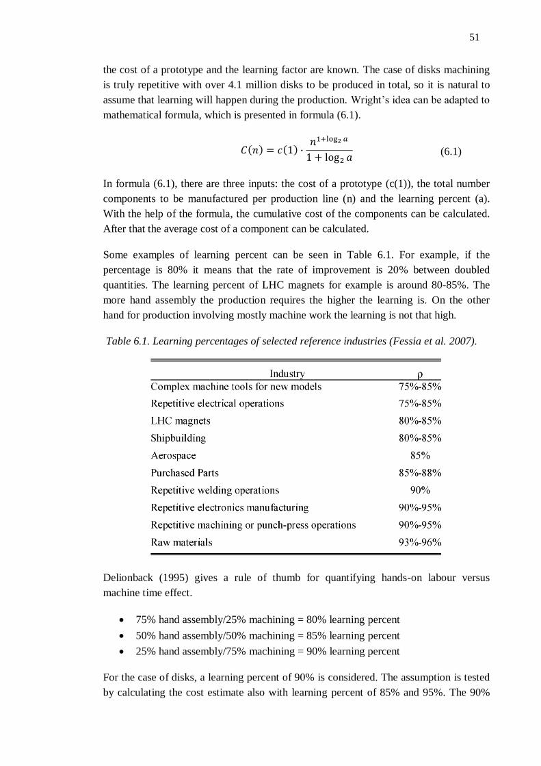
51
the cost of a prototype and the learning factor are known. The case of disks machining
is truly repetitive with over 4.1 million disks to be produced in total, so it is natural to
assume that learning will happen during the production. Wright’s idea can be adapted to
mathematical formula, which is presented in formula (6.1).
(6.1)
In formula (6.1), there are three inputs: the cost of a prototype (c(1)), the total number
components to be manufactured per production line (n) and the learning percent (a).
With the help of the formula, the cumulative cost of the components can be calculated.
After that the average cost of a component can be calculated.
Some examples of learning percent can be seen in Table 6.1. For example, if the
percentage is 80% it means that the rate of improvement is 20% between doubled
quantities. The learning percent of LHC magnets for example is around 80-85%. The
more hand assembly the production requires the higher the learning is. On the other
hand for production involving mostly machine work the learning is not that high.
Table 6.1. Learning percentages of selected reference industries (Fessia et al. 2007).
Delionback (1995) gives a rule of thumb for quantifying hands-on labour versus
machine time effect.
75% hand assembly/25% machining = 80% learning percent
50% hand assembly/50% machining = 85% learning percent
25% hand assembly/75% machining = 90% learning percent
For the case of disks, a learning percent of 90% is considered. The assumption is tested
by calculating the cost estimate also with learning percent of 85% and 95%. The 90%
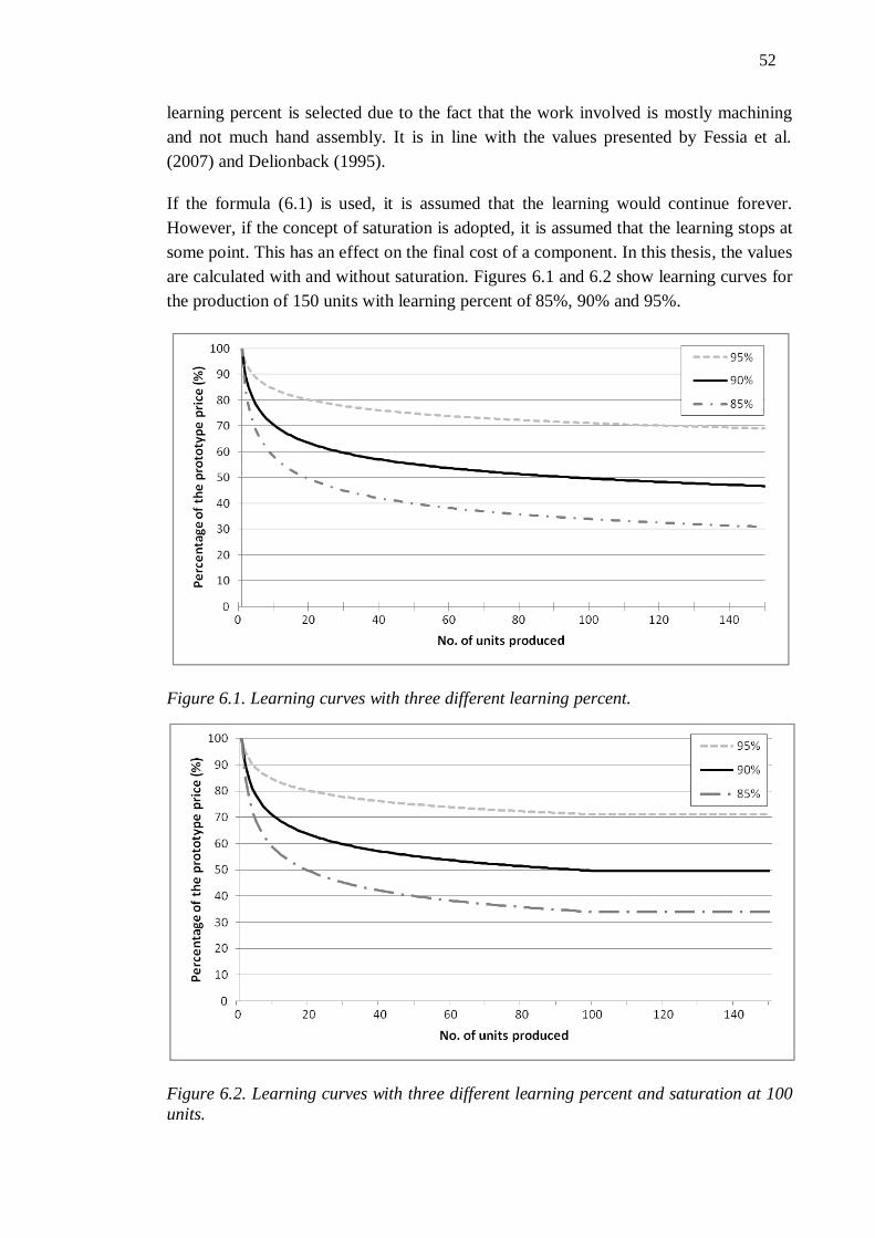
52
learning percent is selected due to the fact that the work involved is mostly machining
and not much hand assembly. It is in line with the values presented by Fessia et al.
(2007) and Delionback (1995).
If the formula (6.1) is used, it is assumed that the learning would continue forever.
However, if the concept of saturation is adopted, it is assumed that the learning stops at
some point. This has an effect on the final cost of a component. In this thesis, the values
are calculated with and without saturation. Figures 6.1 and 6.2 show learning curves for
the production of 150 units with learning percent of 85%, 90% and 95%.
Figure 6.1. Learning curves with three different learning percent.
Figure 6.2. Learning curves with three different learning percent and saturation at 100
units.
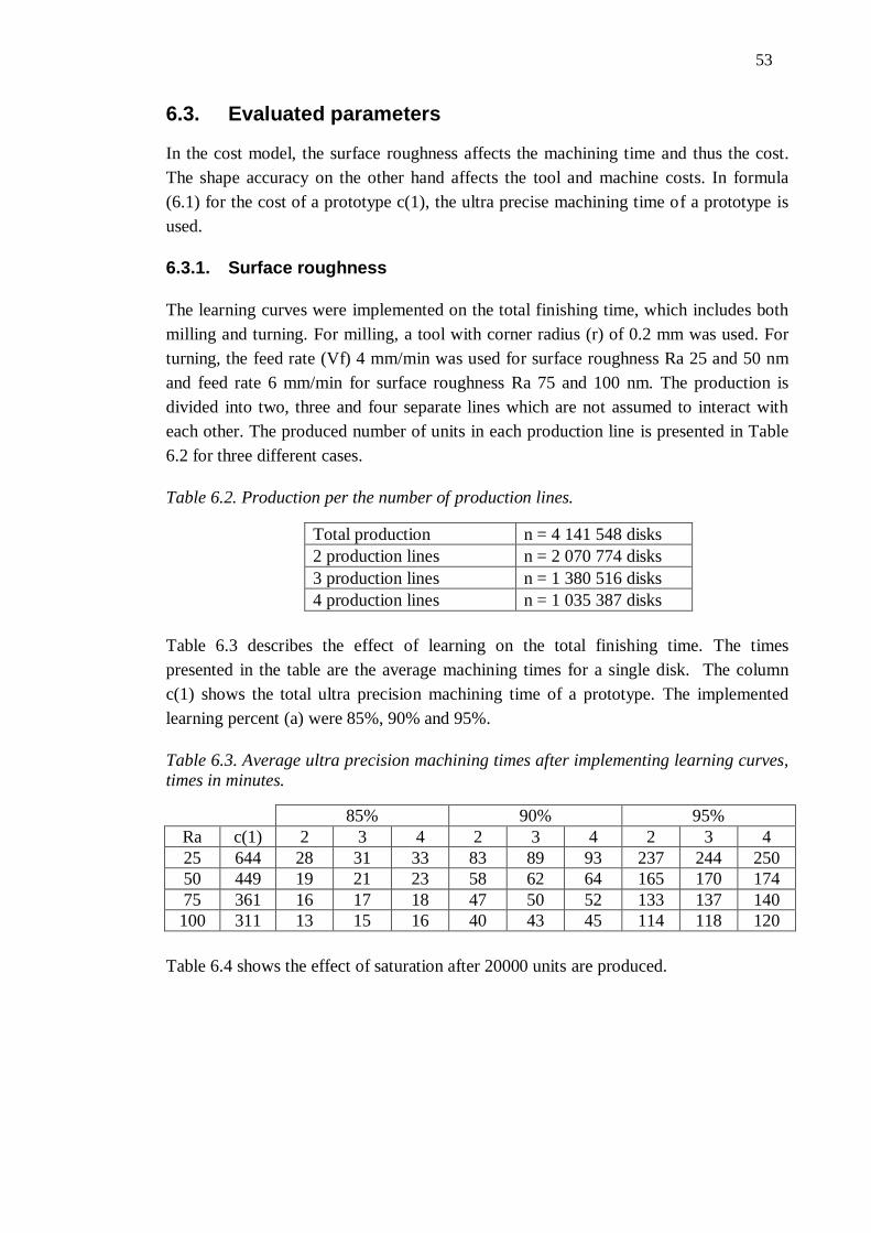
53
6.3. Evaluated parameters
In the cost model, the surface roughness affects the machining time and thus the cost.
The shape accuracy on the other hand affects the tool and machine costs. In formula
(6.1) for the cost of a prototype c(1), the ultra precise machining time of a prototype is
used.
6.3.1. Surface roughness
The learning curves were implemented on the total finishing time, which includes both
milling and turning. For milling, a tool with corner radius (r) of 0.2 mm was used. For
turning, the feed rate (Vf) 4 mm/min was used for surface roughness Ra 25 and 50 nm
and feed rate 6 mm/min for surface roughness Ra 75 and 100 nm. The production is
divided into two, three and four separate lines which are not assumed to interact with
each other. The produced number of units in each production line is presented in Table
6.2 for three different cases.
Table 6.2. Production per the number of production lines.
Total production n = 4 141 548 disks
2 production lines n = 2 070 774 disks
3 production lines n = 1 380 516 disks
4 production lines n = 1 035 387 disks
Table 6.3 describes the effect of learning on the total finishing time. The times
presented in the table are the average machining times for a single disk. The column
c(1) shows the total ultra precision machining time of a prototype. The implemented
learning percent (a) were 85%, 90% and 95%.
Table 6.3. Average ultra precision machining times after implementing learning curves,
times in minutes.
85% 90% 95%
Ra c(1) 2 3 4 2 3 4 2 3 4
25 644 28 31 33 83 89 93 237 244 250
50 449 19 21 23 58 62 64 165 170 174
75 361 16 17 18 47 50 52 133 137 140
100 311 13 15 16 40 43 45 114 118 120
Table 6.4 shows the effect of saturation after 20000 units are produced.
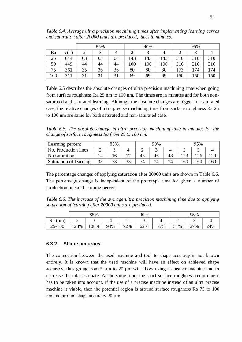
54
Table 6.4. Average ultra precision machining times after implementing learning curves
and saturation after 20000 units are produced, times in minutes.
85% 90% 95%
Ra c(1) 2 3 4 2 3 4 2 3 4
25 644 63 63 64 143 143 143 310 310 310
50 449 44 44 44 100 100 100 216 216 216
75 361 35 36 36 80 80 80 173 174 174
100 311 31 31 31 69 69 69 150 150 150
Table 6.5 describes the absolute changes of ultra precision machining time when going
from surface roughness Ra 25 nm to 100 nm. The times are in minutes and for both non-
saturated and saturated learning. Although the absolute changes are bigger for saturated
case, the relative changes of ultra precise machining time from surface roughness Ra 25
to 100 nm are same for both saturated and non-saturated case.
Table 6.5. The absolute change in ultra precision machining time in minutes for the
change of surface roughness Ra from 25 to 100 nm.
Learning percent 85% 90% 95%
No. Production lines 2 3 4 2 3 4 2 3 4
No saturation 14 16 17 43 46 48 123 126 129
Saturation of learning 33 33 33 74 74 74 160 160 160
The percentage changes of applying saturation after 20000 units are shown in Table 6.6.
The percentage change is independent of the prototype time for given a number of
production line and learning percent.
Table 6.6. The increase of the average ultra precision machining time due to applying
saturation of learning after 20000 units are produced.
85% 90% 95%
Ra (nm) 2 3 4 2 3 4 2 3 4
25-100 128% 108% 94% 72% 62% 55% 31% 27% 24%
6.3.2. Shape accuracy
The connection between the used machine and tool to shape accuracy is not known
entirely. It is known that the used machine will have an effect on achieved shape
accuracy, thus going from 5 µm to 20 µm will allow using a cheaper machine and to
decrease the total estimate. At the same time, the strict surface roughness requirement
has to be taken into account. If the use of a precise machine instead of an ultra precise
machine is viable, then the potential region is around surface roughness Ra 75 to 100
nm and around shape accuracy 20 µm.
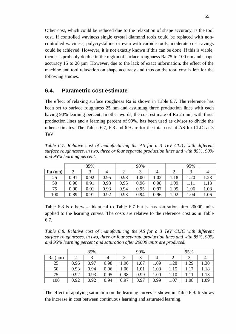
55
Other cost, which could be reduced due to the relaxation of shape accuracy, is the tool
cost. If controlled waviness single crystal diamond tools could be replaced with non-
controlled waviness, polycrystalline or even with carbide tools, moderate cost savings
could be achieved. However, it is not exactly known if this can be done. If this is viable,
then it is probably doable in the region of surface roughness Ra 75 to 100 nm and shape
accuracy 15 to 20 µm. However, due to the lack of exact information, the effect of the
machine and tool relaxation on shape accuracy and thus on the total cost is left for the
following studies.
6.4. Parametric cost estimate
The effect of relaxing surface roughness Ra is shown in Table 6.7. The reference has
been set to surface roughness 25 nm and assuming three production lines with each
having 90% learning percent. In other words, the cost estimate of Ra 25 nm, with three
production lines and a learning percent of 90%, has been used as divisor to divide the
other estimates. The Tables 6.7, 6.8 and 6.9 are for the total cost of AS for CLIC at 3
TeV.
Table 6.7. Relative cost of manufacturing the AS for a 3 TeV CLIC with different
surface roughnesses, in two, three or four separate production lines and with 85%, 90%
and 95% learning percent.
85% 90% 95%
Ra (nm) 2 3 4 2 3 4 2 3 4
25 0.91 0.92 0.95 0.98 1.00 1.02 1.18 1.20 1.23
50 0.90 0.91 0.93 0.95 0.96 0.98 1.09 1.11 1.13
75 0.90 0.91 0.93 0.94 0.95 0.97 1.05 1.06 1.08
100 0.89 0.91 0.92 0.93 0.94 0.96 1.02 1.04 1.06
Table 6.8 is otherwise identical to Table 6.7 but is has saturation after 20000 units
applied to the learning curves. The costs are relative to the reference cost as in Table
6.7.
Table 6.8. Relative cost of manufacturing the AS for a 3 TeV CLIC with different
surface roughnesses, in two, three or four separate production lines and with 85%, 90%
and 95% learning percent and saturation after 20000 units are produced.
85% 90% 95%
Ra (nm) 2 3 4 2 3 4 2 3 4
25 0.96 0.97 0.98 1.06 1.07 1.09 1.28 1.29 1.30
50 0.93 0.94 0.96 1.00 1.01 1.03 1.15 1.17 1.18
75 0.92 0.93 0.95 0.98 0.99 1.00 1.10 1.11 1.13
100 0.92 0.92 0.94 0.97 0.97 0.99 1.07 1.08 1.09
The effect of applying saturation on the learning curves is shown in Table 6.9. It shows
the increase in cost between continuous learning and saturated learning.

56
Table 6.9. The effect of applying saturation of learning to the total cost estimate for the
AS for a 3 TeV CLIC.
85% 90% 95%
Ra (nm) 2 3 4 2 3 4 2 3 4
25 5% 4% 4% 8% 7% 7% 8% 7% 6%
50 4% 3% 3% 6% 5% 5% 6% 5% 5%
75 3% 3% 2% 5% 4% 4% 5% 4% 4%
100 2% 2% 2% 4% 3% 4% 5% 4% 3%
It can be seen in Table 6.9 that decreasing the number of production lines increases the
total cost due to saturation. The smaller the learning percent is the less of an impact the
saturation has.
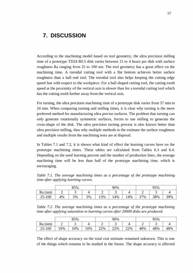
57
7. DISCUSSION
According to the machining model based on tool geometry, the ultra precision milling
time of a prototype TD24 R0.5 disk varies between 15 to 4 hours per disk with surface
roughness Ra ranging from 25 to 100 nm. The tool geometry has a great effect on the
machining time. A toroidal cutting tool with a flat bottom achieves better surface
roughness than a ball end tool. The toroidal tool also helps keeping the cutting edge
speed fast with respect to the workpiece. For a ball shaped cutting tool, the cutting tooth
speed at the proximity of the vertical axis is slower than for a toroidal cutting tool which
has the cutting tooth further away from the vertical axis.
For turning, the ultra precision machining time of a prototype disk varies from 37 min to
24 min. When comparing turning and milling times, it is clear why turning is the more
preferred method for manufacturing ultra precise surfaces. The problem that turning can
only generate rotationally symmetric surfaces, forces to use milling to generate the
cross-shape of the disk. The ultra precision turning process is also known better than
ultra precision milling, thus why multiple methods to the estimate the surface roughness
and multiple results from the machining tests are at disposal.
In Tables 7.1 and 7.2, it is shown what kind of effect the learning curves have on the
prototype machining times. These tables are calculated from Tables 6.3 and 6.4.
Depending on the used learning percent and the number of production lines, the average
machining time will be less than half of the prototype machining time, which is
encouraging.
Table 7.1. The average machining times as a percentage of the prototype machining
time after applying learning curves.
85% 90% 95%
Ra (nm) 2 3 4 2 3 4 2 3 4
25-100 4% 5% 5% 13% 14% 14% 37% 38% 39%
Table 7.2. The average machining times as a percentage of the prototype machining
time after applying saturation to learning curves after 20000 disks are produced.
85% 90% 95%
Ra (nm) 2 3 4 2 3 4 2 3 4
25-100 10% 10% 10% 22% 22% 22% 48% 48% 48%
The effect of shape accuracy on the total cost estimate remained unknown. This is one
of the things which remains to be studied in the future. The shape accuracy is affected
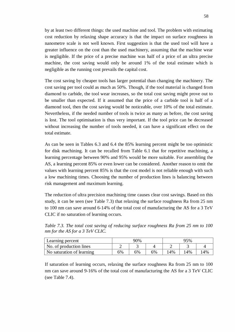
58
by at least two different things: the used machine and tool. The problem with estimating
cost reduction by relaxing shape accuracy is that the impact on surface roughness in
nanometre scale is not well known. First suggestion is that the used tool will have a
greater influence on the cost than the used machinery, assuming that the machine wear
is negligible. If the price of a precise machine was half of a price of an ultra precise
machine, the cost saving would only be around 1% of the total estimate which is
negligible as the running cost prevails the capital cost.
The cost saving by cheaper tools has larger potential than changing the machinery. The
cost saving per tool could as much as 50%. Though, if the tool material is changed from
diamond to carbide, the tool wear increases, so the total cost saving might prove out to
be smaller than expected. If it assumed that the price of a carbide tool is half of a
diamond tool, then the cost saving would be noticeable, over 10% of the total estimate.
Nevertheless, if the needed number of tools is twice as many as before, the cost saving
is lost. The tool optimisation is thus very important. If the tool price can be decreased
without increasing the number of tools needed, it can have a significant effect on the
total estimate.
As can be seen in Tables 6.3 and 6.4 the 85% learning percent might be too optimistic
for disk machining. It can be recalled from Table 6.1 that for repetitive machining, a
learning percentage between 90% and 95% would be more suitable. For assembling the
AS, a learning percent 85% or even lower can be considered. Another reason to omit the
values with learning percent 85% is that the cost model is not reliable enough with such
a low machining times. Choosing the number of production lines is balancing between
risk management and maximum learning.
The reduction of ultra precision machining time causes clear cost savings. Based on this
study, it can be seen (see Table 7.3) that relaxing the surface roughness Ra from 25 nm
to 100 nm can save around 6-14% of the total cost of manufacturing the AS for a 3 TeV
CLIC if no saturation of learning occurs.
Table 7.3. The total cost saving of reducing surface roughness Ra from 25 nm to 100
nm for the AS for a 3 TeV CLIC.
Learning percent 90% 95%
No. of production lines 2 3 4 2 3 4
No saturation of learning 6% 6% 6% 14% 14% 14%
If saturation of learning occurs, relaxing the surface roughness Ra from 25 nm to 100
nm can save around 9-16% of the total cost of manufacturing the AS for a 3 TeV CLIC
(see Table 7.4).
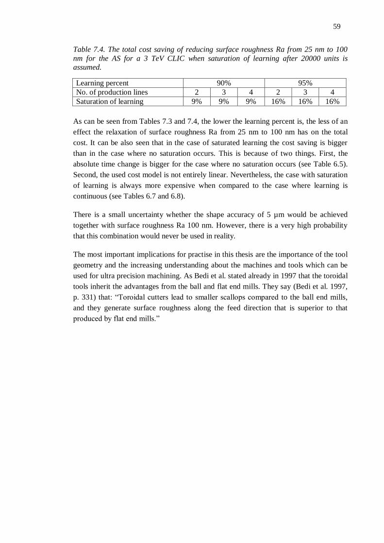
59
Table 7.4. The total cost saving of reducing surface roughness Ra from 25 nm to 100
nm for the AS for a 3 TeV CLIC when saturation of learning after 20000 units is
assumed.
Learning percent 90% 95%
No. of production lines 2 3 4 2 3 4
Saturation of learning 9% 9% 9% 16% 16% 16%
As can be seen from Tables 7.3 and 7.4, the lower the learning percent is, the less of an
effect the relaxation of surface roughness Ra from 25 nm to 100 nm has on the total
cost. It can be also seen that in the case of saturated learning the cost saving is bigger
than in the case where no saturation occurs. This is because of two things. First, the
absolute time change is bigger for the case where no saturation occurs (see Table 6.5).
Second, the used cost model is not entirely linear. Nevertheless, the case with saturation
of learning is always more expensive when compared to the case where learning is
continuous (see Tables 6.7 and 6.8).
There is a small uncertainty whether the shape accuracy of 5 µm would be achieved
together with surface roughness Ra 100 nm. However, there is a very high probability
that this combination would never be used in reality.
The most important implications for practise in this thesis are the importance of the tool
geometry and the increasing understanding about the machines and tools which can be
used for ultra precision machining. As Bedi et al. stated already in 1997 that the toroidal
tools inherit the advantages from the ball and flat end mills. They say (Bedi et al. 1997,
p. 331) that: “Toroidal cutters lead to smaller scallops compared to the ball end mills,
and they generate surface roughness along the feed direction that is superior to that
produced by flat end mills.”
60
8. CONCLUSIONS
The disks used in CLIC two-beam AS are made out of copper by turning and milling.
The strict nominal tolerance requirements for surface roughness Ra, 25 nm, and shape
accuracy, 5 µm, are the reasons for the need of ultra precision machining. The
machining is done in many passes starting from pre-machining and ending with ultra
precise machining in order to achieve the specifications. The facts that at the moment
the ultra precision machining is taking around 10 hours per disk with the presented
parameters, and that in CLIC at 3 TeV, 4.1 million disks will be needed, are the reasons
why machining time is an important cost driver also in the scale of the whole CLIC
project.
The huge number of disks to be machined suggests that inevitably innovations and
streamlining of processes will occur during the project. In the cost calculations, this is
taken into account in the form of Wright’s (1936) learning curves. A learning percent of
90%, which is typical for repetitive machining, was applied. Although the total
production is divided into separate production lines and no collective innovation is
expected, the average times for ultra precision machining are nevertheless promising.
The fact that the disks should be machined to a precision of a few µm or even less will
demand adequate machines to verify the measurements. Those machines nowadays
exist but the problem is that verifying every disk by a contact measurement machine
takes time, thus why only some statistical samples would be verified in the production
of CLIC.
The average ultra precise machining times after applying learning curves with no
saturation and learning percent of 90% and 95% were between 83 and 250 minutes for
surface roughness Ra 25 nm. For surface roughness Ra 100 nm, the similar values were
from 40 to 120 minutes. Assuming a saturation of learning after 20000 disks are
produced, the total times are from 143 to 310 minutes for surface roughness Ra 25 nm.
For surface roughness Ra 100 nm, the times are from 69 to 150 minutes. Total cost
saving in the two-bean accelerating structures when relaxing the surface roughness Ra
from 25 nm to 100 nm is between 6% and 16% whereas the effect of relaxing shape
accuracy remained unclear.
In the future, also other methods than mechanical machining have to be considered for
manufacturing the disks. There are already a few known methods which could be used
instead of mechanical machining. Figure 8.1 shows different types of methods in
addition to mechanical machining. For the moment, none of those methods is ready to
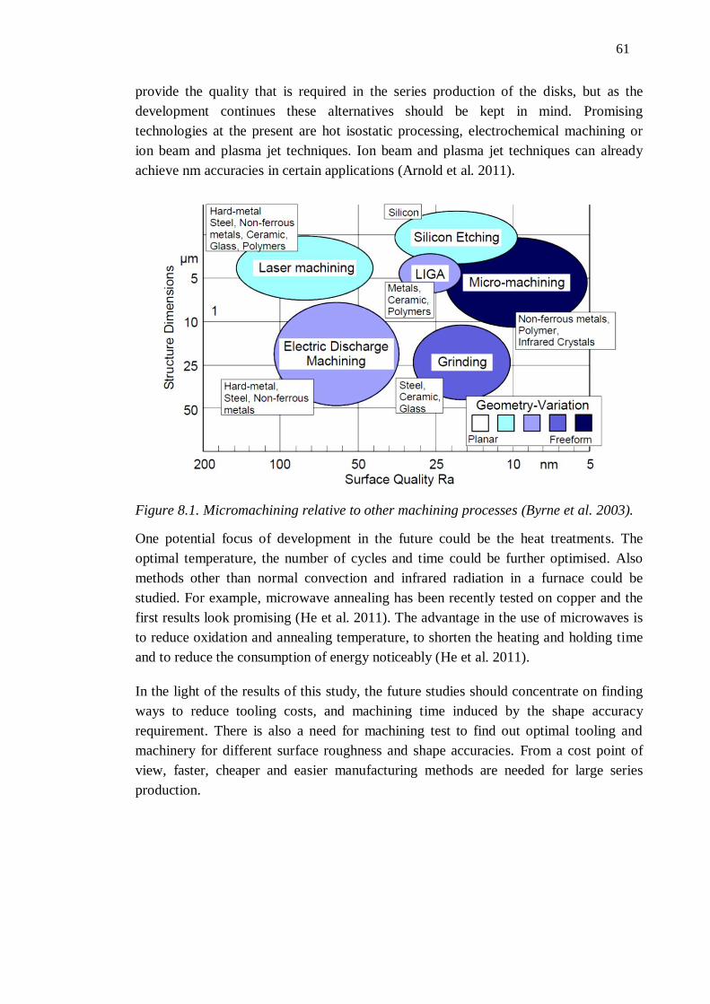
61
provide the quality that is required in the series production of the disks, but as the
development continues these alternatives should be kept in mind. Promising
technologies at the present are hot isostatic processing, electrochemical machining or
ion beam and plasma jet techniques. Ion beam and plasma jet techniques can already
achieve nm accuracies in certain applications (Arnold et al. 2011).
Figure 8.1. Micromachining relative to other machining processes (Byrne et al. 2003).
One potential focus of development in the future could be the heat treatments. The
optimal temperature, the number of cycles and time could be further optimised. Also
methods other than normal convection and infrared radiation in a furnace could be
studied. For example, microwave annealing has been recently tested on copper and the
first results look promising (He et al. 2011). The advantage in the use of microwaves is
to reduce oxidation and annealing temperature, to shorten the heating and holding time
and to reduce the consumption of energy noticeably (He et al. 2011).
In the light of the results of this study, the future studies should concentrate on finding
ways to reduce tooling costs, and machining time induced by the shape accuracy
requirement. There is also a need for machining test to find out optimal tooling and
machinery for different surface roughness and shape accuracies. From a cost point of
view, faster, cheaper and easier manufacturing methods are needed for large series
production.
62
BIBLIOGRAPHY
Angus, J. C. 2002. A short history of diamond synthesis. In: Diamond films handbook.
Editors: Asmussen, J. & Reinhard, D. K. Marcel Dekker.
Arnold, T., Böhm, G., Fechner, R., Meister, J., Nickel, A., Frost, F., Hänsel, T. & Schindler,
A. 2010. Ultra-Precision Surface Finishing by Ion Beam and Plasma Jet
techniques—status and Outlook. Nuclear Instruments and Methods in Physics
Research Section A: Accelerators, Spectrometers, Detectors and Associated
Equipment. Vol. 616(2-3), pp. 147-156.
ASM International Handbook Committee 1991. ASM handbook, volume 4 - heat treating.
ASM International. 1012 p.
ASM International Handbook Committee 1989. ASM handbook, volume 16 - machining.
ASM International. 944 p.
Atieh, S., Aicheler, M., Arnau-Izquierdo, G., Cherif, A., Deparis, L., Glaude, D., Remandet,
L., Riddone, G., Scheubel, G., Gudkov, D., Samoshkin, A. & Solodko, A. 2011.
Machining and Characterizing x-Band RF-Structures for CLIC. Proceedings of the
2nd International Particle Accelerator Conference. San Sebastian, Spain, 4-9
September 2011.
Baptista, R. & Antune Simões, J. F. 2000. Three and Five Axes Milling of Sculptured
Surfaces. Journal of Materials Processing Technology. Vol. 103(3), pp. 398-403.
Bedi, S., Ismail, F., Mahjoob, M. J. & Chen, Y. 1997. Toroidal Versus Ball Nose and Flat
Bottom End Mills. The International Journal of Advanced Manufacturing
Technology. Vol. 13(5), pp. 326-332.
Benardos, P. G. & Vosniakos, G.-C. 2003. Predicting Surface Roughness in Machining: A
Review. International Journal of Machine Tools and Manufacture. Vol. 43(8), pp.
833-844.
Black, S. C., Chiles, V., Lissaman, A. J. & Martill, S. J. 1996. Principles of engineering
manufacture. 3rd ed. Oxford: Butterworth-Heinemann. 656 p.
Brammertz, P. H. 1961. Die Entstehung Der Oberflächenrauheit Beim Feindrehen.
Industrie-Anzeiger. Vol. 83(2), pp. 25-32.
Braun, H., Corsini, R., Delahaye, J., de Roeck, A., Döbert, S., Ferrari, A., Geschonke, G.,
Grudiev, A., Hauviller, C., Jeanneret, B., Jensen, E., Lefèvre, T., Papaphilippou, Y.,
Riddone, G., Rinolfi, L., Schlatter, W. D., Schmickler, H., Schulte, D., Syratchev,
I., Taborelli, M., Tecker, F., Tomás, R., Weisz, S. & Wuensch, W. 2008a. CLIC
2008 Parameters.
Braun, H., Delahaye, J., De Roeck, A. & Geschonke, G. 2008b. CLIC here for the Future.
CERN Courier. Vol. September, pp. 15-18.
Brecher, C., Lange, S., Merz, M., Niehaus, F. & Winterschladen, M. 2006. Off-axis
machining of NURBS freeform surfaces by fast tool servo systems. In: 4M 2006 -
63
second international conference on multi-material micro manufacture. Editors:
Wolfgang Menz, Stefan Dimov & Bertrand Fillon. Elsevier, Oxford. pp. 59-62.
Byrne, G., Dornfeld, D. & Denkena, B. 2003. Advancing Cutting Technology. CIRP Annals
- Manufacturing Technology. Vol. 52(2), pp. 483-507.
CDA 2011. Copper Development Association. Website. Available: www.copper.org.
Referred: 9.5.2011.
CERN 2011. CERN – the European Organization for Nuclear Research. Website.
Available: www.cern.ch. Referred: 4.4.2011.
CERN Bulletin 2011. Measuring past a micron. Available:
http://cdsweb.cern.ch/journal/CERNBulletin/2011/31/News Articles/1364613/.
CFT 2011. Countour Fine Tooling Limited. Website. Available: www.contour-
diamonds.com. Referred: 13.5.2011.
Chandler, H. 1996. Heat treater's guide - practices and procedures for nonferrous alloys.
ASM International. 669 p.
Chardontool, 2011. About diamond – What is polycrystalline diamond? Webpage.
Available: www.chardontool.com. Referred: 11.7.2011.
Cherif, A. 2011. Dimensional control. Presentation on CLIC MeChanICs project meeting.
22.3.2011.
Cheung, C. F. & Lee, W. B. 2000. A Theoretical and Experimental Investigation of Surface
Roughness Formation in Ultra-Precision Diamond Turning. International Journal of
Machine Tools and Manufacture. Vol. 40(7), pp. 979-1002.
Corbett, J., McKeown, P. A., Peggs, G. N. & Whatmore, R. 2000. Nanotechnology:
International Developments and Emerging Products. CIRP Annals-Manufacturing
Technology. Vol. 49(2), pp. 523-545.
CTF3 2011. CLIC Test Facility 3. Website. Available: http://ctf3.home.cern.ch/. Referred:
4.4.2011.
CustomPartNet 2011. Website. Available: www.custompartnet.com. Referred: 14.6.2011.
Delionback, L. M. 1995. Learning curves and progress functions. In: Cost estimator's
reference manual. Editors: Stewart, R. D., Wyskida, R. M. & Johannes, J. D. 2nd
ed. John Wiley & Sons, Inc., New York, NY. pp. 169-192.
DKI 2010. Recommended machining parameters for copper and copper alloys. Monograph
i.18. German Copper Institute, Düsseldorf, Germany. 64 p.
Döbert, S., Grudiev, A., Riddone, G., Wuensch, W., Zennaro, R., Higo, T., Matsumoto, S.,
Yokoyama, K., Adolphsen, C., Wang, F.& Wang, J. 2010. First High Power Tests
of Clic Prototype Accelerating Structures with Hom Waveguide Damping. Geneva:
CERN. CERN-ATS-2010-204.
Elepano, J. 2010. Optical CMMs: The future of CMMs? Quality Digest Magazine.
Fessia, P., Regis, F. & Rossi, L. 2007. Industrial Learning Curves: Series Production of
the LHC Main Superconducting Dipoles. Applied Superconductivity, IEEE
Transactions on. Vol. 17(2), pp. 1101-1104.
Filiz, S., Conley, C. M., Wasserman, M. B. & Ozdoganlar, O. B. 2007. An Experimental
Investigation of Micro-Machinability of Copper 101 using Tungsten Carbide
Micro-Endmills. International Journal of Machine Tools and Manufacture. Vol.
47(7-8), pp. 1088-1100.
64
Galli, G. & Raty, J. 2004. Nanodiamonds. In: Dekker encyclopedia of nanoscience and
nanotechnology - six volume set (print version). Editors: Schwarz, J. A. &
Contescu, C. I. Marcel Dekker Inc.
Geng, H. 2004. Manufacturing engineering handbook. McGraw-Hill. 1176 p.
Grzesik, W. 2008. Advanced machining processes of metallic materials - theory, modelling
and applications. Amsterdam; Boston; London: Elsevier. 472 p.
Haberland, R., Böffgen, M. & Klein, W. 1996. Neue Verschleißerscheinungen an
Monokristallinen Diamantwerkzeugen. Industrie Diamanten Rundschau. Vol. 30(2),
pp. 72-73.
Hamada, H. 1985. Diamond Tools for Ultra-Precision Machining. Journal of the Japan
Society of Precision Engineering. Vol. 51(9), pp. 1669-1673.
Haynes, W. M. 2010-2011. Properties of solids. in CRC Handbook of Chemistry and
Physic. 91st ed. Boca Raton, FL: CRC Press/Taylor and Francis.
He, W., Ai, Y. L., Ding, J. Y., Liu, L. & He, F. 2011. Microwave Annealing of Cold
Compression Deformation Red Copper. Advanced Materials Research. Vol. 199-
200, pp. 1840-1844.
Huo, D. & Cheng, K. 2010. Experimental Investigation on Micromilling of Oxygen-Free,
High-Conductivity Copper using Tungsten Carbide, Chemistry Vapour Deposition,
and Single-Crystal Diamond Micro Tools. Proceedings of the Institution of
Mechanical Engineers, Part B: Journal of Engineering Manufacture. Vol. 224(6),
pp. 995-1003.
Huo, D., Cheng, K. & Wardle, F. 2010. Design of a Five-Axis Ultra-Precision Micro-
Milling machine—UltraMill. Part 1: Holistic Design Approach, Design
Considerations and Specifications. The International Journal of Advanced
Manufacturing Technology. Vol. 47(9), pp. 867-877.
Hwang, J., Kim, K., Won, J. & Chung, E. 2008. Ultraprecision Cavity Fabrication of High-
Power Klystron Amplifier Tube for PLS Linear Accelerator. Proceedings of
Nano/Micro Engineered and Molecular Systems, 2008. NEMS 2008. 3rd IEEE
International Conference on. pp. 1053-1058.
ILC 2011. International Linear Collider. Website. Available: www.linearcollider.org/.
Referred 27.4.2011.
ISO 1101:2004(E) 2004. Geometrical Product Specifications (GPS) - Geometrical
tolerancing - Tolerances of form, orientation, location and run-out. Internal
Organization for Standardization. 54 p.
ISO 4287:1997(E) 1997. Geometrical Product Specifications (GPS) – Surface texture:
Profile method - Terms, definitions, and surface texture parameters. Internal
Organization for Standardization. 25 p.
Jawaid, A., Sharif, S. & Koksal, S. 2000. Evaluation of Wear Mechanisms of Coated
Carbide Tools when Face Milling Titanium Alloy. Journal of Materials Processing
Technology. Vol. 99(1-3), pp. 266-274.
Jolic, K. I., Nagarajah, C. R. & Thompson, W. 1994. Non-Contact, Optically Based
Measurement of Surface Roughness of Ceramics. Measurement Science and
Technology. Vol. 5(6), pp. 671-684.
Khan, G. S., Sarepaka, R. G. V., Chattopadhyay, K. D., Jain, P. K. & Bajpai, R. P. 2004.
Characterization of Nanoscale Roughness in Single Point Diamond Turned Optical
65
Surfaces using Power Spectral Density Analysis. Indian Journal of Engineering and
Materials Science. Vol. 11(1), pp. 25-30.
Kim, B. H. & Chu, C. N. 1999. Texture Prediction of Milled Surfaces using Texture
Superposition Method. Computer-Aided Design. Vol. 31(8), pp. 485-494.
Knuefermann, M. M. W. & McKeown, P. A. 2004. A Model for Surface Roughness in
Ultraprecision Hard Turning. CIRP Annals - Manufacturing Technology. Vol.
53(1), pp. 99-102.
Krizbergs, J. & Kromanis, A. Methods for Prediction of the Surface Roughness 3D
Parameters According to Technological Parameters. Proceedings of 5th
International DAAAM Baltic Conference. Tallinn, Estonia, 20 - 22 April 2006.
Leitz 2011. Leitz PMM-C Infinity. Webpage. Available: www.leitz-
metrology.com/541.htm. Referred: 29.3.2011.
Li, H., Lai, X., Li, C., Feng, J. & Ni, J. 2008. Modelling and Experimental Analysis of the
Effects of Tool Wear, Minimum Chip Thickness and Micro Tool Geometry on the
Surface Roughness in Micro-End-Milling. Journal of Micromechanics and
Microengineering. Vol. 18(2), pp. 1-12.
Lucca, D. A., Rhorer, R. L. & Komanduri, R. 1991. Energy Dissipation in the
Ultraprecision Machining of Copper. CIRP Annals - Manufacturing Technology.
Vol. 40(1), pp. 69-72.
Luo, X., Cheng, K., Webb, D. & Wardle, F. 2005. Design of Ultraprecision Machine Tools
with Applications to Manufacture of Miniature and Micro Components. Journal of
Materials Processing Technology. Vol. 167(2-3), pp. 515-528.
Mamalis, A. G., Grabchenko, A. I., Horváth, M., Mészáros, I. & Paulmier, D. 2001.
Ultraprecision Metal Removal Processing of Mirror-Surfaces. Journal of Materials
Processing Technology. Vol. 108(3), pp. 269-277.
Medicus, K. M., Davies, M. A., Dutterer, B. S., Evans, C. J. & Fielder, R. S. 2001. Tool
Wear and Surface Finish in High Speed Milling of Aluminum Bronze. Machining
Science and Technology: An International Journal. Vol. 5(2), pp. 255-268.
Mills, B. & Redford, A. H. 1983. Machinability of engineering materials. London: Applied
Science Publishers. 174 p.
Miyoshi, K. 2001. Structures and mechanical properties of natural and synthetic diamond.
In: Solid lubrication fundamentals and applications. Editor: Miyoshi, K. 1st ed.
Marcel Dekker Inc, New York, USA. 21 p.
Morehead, M., Huang, Y. & Ted Hartwig, K. 2007. Machinability of Ultrafine-Grained
Copper using Tungsten Carbide and Polycrystalline Diamond Tools. International
Journal of Machine Tools and Manufacture. Vol. 47(2), pp. 286-293.
Quintana, G., Ciurana, J. d. & Ribatallada, J. 2010. Surface Roughness Generation and
Material Removal Rate in Ball End Milling Operations. Materials and
Manufacturing Processes. Vol. 25(6), pp. 386-398.
Reinecke, H. & Müller, C. 2008. Micromachining. In: Comprehensive microsystems.
Editors: Gianchandani, Y., Tabata, O. & Zappe, H. Elsevier, Oxford. pp. 379-402.
Riddone, G., Mainaud-Durand, H., Nousiainen, R., Samoshkin, A., Schulte, D., Syratchev,
I., Wuensch, W. & Zennaro, R. 2008. Technical Specification for the CLIC Two-
66
Beam Module. Proceedings of EPAC08. Genoa, Italy, 23-27 June 2008. pp. 607-
609.
Riddone, G. 2010. Engineering aspects and technical systems of CLIC RF structures.
Presentation in the International Workshop on Linear Colliders 2010. Geneva,
Switzerland, 18-22 October 2010.
Riddone, G., Samoshkin, A. & Gudkov, D. 2010. CLIC Two-Beam Module Design and
Integration. Proceedings of the 25th International Linear Accelerator Conference.
Tsukuba, Japan, 12-17 September 2010.
Samoshkin, A. 2008. CLIC Module Integration. Presentation in Mini-Workshop on Girder,
Components Supports and Alignment Concept, 4.12.2008. Paul Scherrer Institute.
Samoshkin, A. 2011. Technical requirements and engineering design of the RF structures.
Presentation in MeChaniCs project meeting. 22.3.2011.
Samoshkin, A., Gudkov, D., Solodko, A. & Riddone, G. 2011. CLIC Two-Beam Module
for the CLIC Conceptual Design and Related Experimental Program. Proceedings
of the 2nd International Particle Accelerator Conference. San Sebastian, Spain, 4-9
September 2011.
Solodko, A., Samoshkin, A., Gudkov, D., Riddone, G., Grudiev, A. & Atieh, S. 2010.
Engineering design and fabrication of x-band accelerating structures TD24 R05 and
TD24 R05 SiC. Poster presentation in the International Workshop on Linear
Colliders 2010. Geneva, Switzerland, 18-22 October 2010.
Stapnes, S. 2011. CLIC status and plans. Presentation in the International Workshop on
Future Linear Colliders 2011. Granada, Spain, 26-30 September 2011.
Son, S. M., Lim, H. S. & Ahn, J. H. 2005. Effects of the Friction Coefficient on the
Minimum Cutting Thickness in Micro Cutting. International Journal of Machine
Tools and Manufacture. Vol. 45(4-5), pp. 529-535.
Sun, X. & Cheng, K. 2010. Chapter 2 - micro-/Nano-machining through mechanical
cutting. In: Micromanufacturing engineering and technology. Editor: Qin, Y.
William Andrew Publishing, Boston. pp. 24-38.
Takamasu, K., Ozawa, S., Asano, T., Suzuki, A., Furutani, R. & Ozono, S. 1996. Basic
Concept of Nano-CMM. Proceedings of Proc. of the Japan-China Bilateral
Symposium on Advanced Manufacturing Engineering. pp. 155-158.
Takeuchi, Y., Yonekura, H. & Sawada, K. 2003. Creation of 3-D Tiny Statue by 5-Axis
Control Ultraprecision Machining. Computer-Aided Design. Vol. 35(4), pp. 403-
409.
Taniguchi, N. 1983. Current Status in, and Future Trends of, Ultraprecision Machining and
Ultrafine Materials Processing. CIRP Annals-Manufacturing Technology. Vol.
32(2), pp. 573-582.
Technodiamant. 2011. Products. Webpage. Available:
www.technodiamant.com/products.htm. Referred: 3.11.2011.
Teitenberg, T. M., Bayoumi, A. E. & Yucesan, G. 1992. Tool Wear Modeling through an
Analytic Mechanistic Model of Milling Processes. Wear. Vol. 154(2), pp. 287-304.
Thomas, T. R. 1999. Rough surfaces. 2nd ed. Singapore: Imperial College. 296 p.
Tomsic, J. L. 2000. Dictionary of materials and testing.2nd ed. Society of Automotive
Engineers, Inc. 442 p.
Uusimäki, T. & Saifoulina, M. 2010. RF structure requirements for industrialization and
mass production cost study. CERN - BE Department. CLIC.
67
Vavrille, J.-L. 2003. Usinage d’ultraprécision. Mecasem Bourgogne.
Veeco 2001. Wyko NT3300 Optical 3D Profiling System – Technical Specifications. Veeco
Metrology Group.
Wang, J., Lewandowski, J., Van Pelt, J., Yoneda, C., Gudkov, D., Riddone, G., Higo, T. &
Takatomi, T. 2010. Fabrication Technologies of the High Gradient Accelerator
Structures at 100MV/m Range. Proceedings of the 1st International Particle
Accelerator Conference. Kyoto, Japan, 23 - 28 May 2010.
Weckenmann, A., Estler, T., Peggs, G. & McMurtry, D. 2004. Probing Systems in
Dimensional Metrology. CIRP Annals - Manufacturing Technology. Vol. 53(2), pp.
657-684.
Whitehouse, D. J. 2002. Handbook of surface and nanometrology. Taylor & Francis. 1150
p.
Wright, T. P. 1936. Factors Affecting the Cost of Airplanes. Journal of the Aeronautical
Sciences. Vol. 3(4), pp. 122-128.
Wuensch, W. 2011. Main linac accelerating system. CLIC Conseptual Design Report.
Forthcoming.
Xu, X. & Hu, H. 2009. Development of Non-Contact Surface Roughness Measurement in
Last Decades. Proceedings of International Conference on Measuring Technology
and Mechatronics Automation, 2009. ICMTMA '09. Zhangjiajie, Hunan, 11-12
April 2009. pp. 210-213.
Yan, J., Syoji, K. & Tamaki, J. 2003. Some Observations on the Wear of Diamond Tools in
Ultra-Precision Cutting of Single-Crystal Silicon. Wear. Vol. 255(7-12), pp. 1380-
1387.
Yan, J., Zhang, Z., Kuriyagawa, T. & Gonda, H. 2010. Fabricating Micro-Structured
Surface by using Single-Crystalline Diamond Endmill. The International Journal
of Advanced Manufacturing Technology. Vol. 51(9), pp. 957-964.
Yoshioka, H. & Shinno, H. 2011. Structural Design of a Newly Developed Ultraprecision
Machine Tool “ANGEL”. Proceedings of International Symposium on
Ultraprecision Engineering and Nanotechnology (ISUPEN). Toyo, Japan, 14-16
March 2011.
Zeiss 2009. State-of-the-art Equipment: Reference Lab for the Nanometer Range. Press
Release from Carl Zeiss. 14.4.2009. PI No.: 0072-2009-ENG. 5 p.
Zennaro, R. 2008a. Study of the Machining and Assembly Tolerances for the CLIC
Accelerating Structure. EUROTeV-Report-2008-081. 10 p.
Zennaro, R. 2008b. Tolerances: Origins, Requirements, Status and Feasibility. Presentation
in the 2nd CLIC Advisory Committee. 17.1.2008.
Zhang, H. & Zhang, X. 1994. Factors Affecting Surface Quality in Diamond Turning of
Oxygen-Free High-Conductance Copper. Applied Optics. Vol. 33(10), pp. 2039-
2042.

68
APPENDICES (4 pieces)
1. CLIAAS110188 CAD drawing.
2. A validated manufacturing flow for ultra precision machining of a disk.
3. A CAD drawing of a toroidal diamond end mill.
4. Matlab code for calculating surface roughness Ra with a given radial depth of cut
Ae and vice-versa.
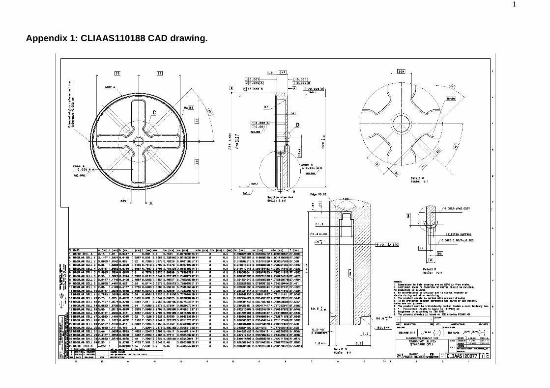
1
Appendix 1: CLIAAS110188 CAD drawing.
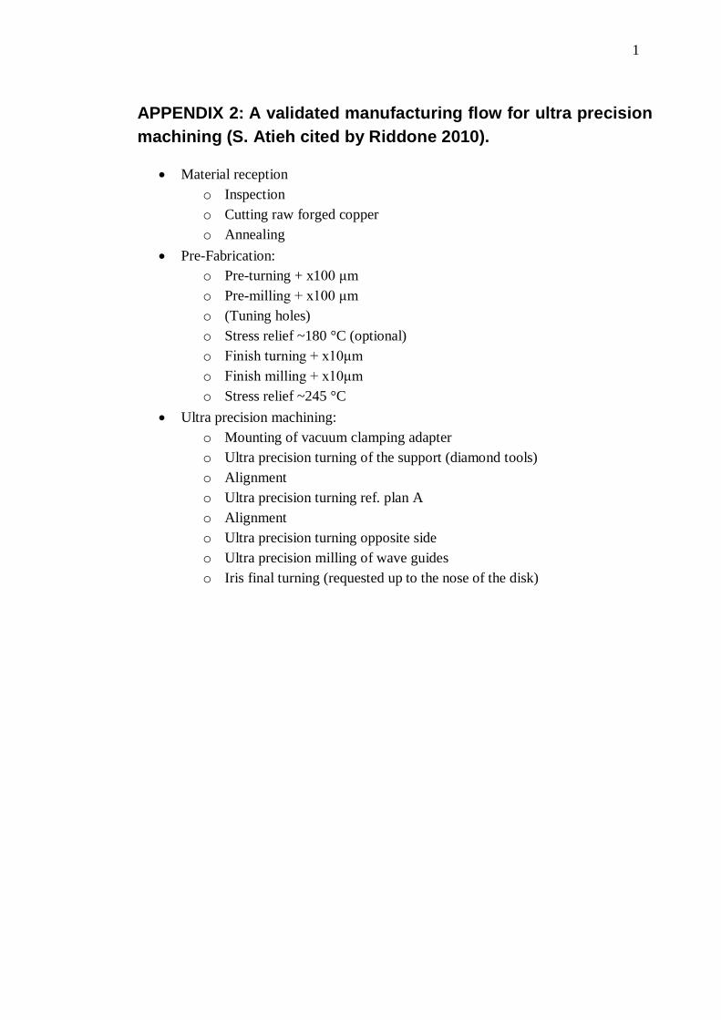
1
APPENDIX 2: A validated manufacturing flow for ultra precision
machining (S. Atieh cited by Riddone 2010).
Material reception
o Inspection
o Cutting raw forged copper
o Annealing
Pre-Fabrication:
o Pre-turning + x100 μm
o Pre-milling + x100 μm
o (Tuning holes)
o Stress relief ~180 °C (optional)
o Finish turning + x10μm
o Finish milling + x10μm
o Stress relief ~245 °C
Ultra precision machining:
o Mounting of vacuum clamping adapter
o Ultra precision turning of the support (diamond tools)
o Alignment
o Ultra precision turning ref. plan A
o Alignment
o Ultra precision turning opposite side
o Ultra precision milling of wave guides
o Iris final turning (requested up to the nose of the disk)
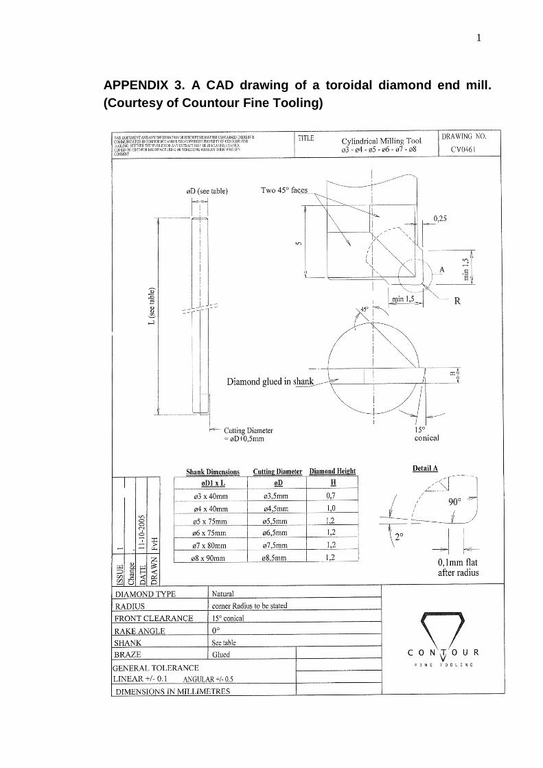
1
APPENDIX 3. A CAD drawing of a toroidal diamond end mill.
(Courtesy of Countour Fine Tooling)
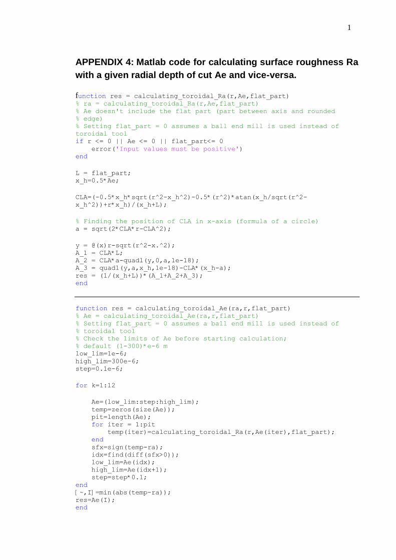
1
APPENDIX 4: Matlab code for calculating surface roughness Ra
with a given radial depth of cut Ae and vice-versa.
function res = calculating_toroidal_Ra(r,Ae,flat_part) % ra = calculating_toroidal_Ra(r,Ae,flat_part) % Ae doesn't include the flat part (part between axis and rounded
% edge)
% Setting flat_part = 0 assumes a ball end mill is used instead of
toroidal tool if r <= 0 || Ae <= 0 || flat_part<= 0 error('Input values must be positive') end
L = flat_part; x_h=0.5*Ae;
CLA=(-0.5*x_h*sqrt(r^2-x_h^2)-0.5*(r^2)*atan(x_h/sqrt(r^2-
x_h^2))+r*x_h)/(x_h+L);
% Finding the position of CLA in x-axis (formula of a circle) a = sqrt(2*CLA*r-CLA^2);
y = @(x)r-sqrt(r^2-x.^2); A_1 = CLA*L; A_2 = CLA*a-quadl(y,0,a,1e-18); A_3 = quadl(y,a,x_h,1e-18)-CLA*(x_h-a); res = (1/(x_h+L))*(A_1+A_2+A_3); end
function res = calculating_toroidal_Ae(ra,r,flat_part) % Ae = calculating_toroidal_Ae(ra,r,flat_part) % Setting flat_part = 0 assumes a ball end mill is used instead of
% toroidal tool
% Check the limits of Ae before starting calculation;
% default (1-300)*e-6 m low_lim=1e-6; high_lim=300e-6; step=0.1e-6;
for k=1:12
Ae=(low_lim:step:high_lim); temp=zeros(size(Ae)); pit=length(Ae); for iter = 1:pit temp(iter)=calculating_toroidal_Ra(r,Ae(iter),flat_part); end sfx=sign(temp-ra); idx=find(diff(sfx>0)); low_lim=Ae(idx); high_lim=Ae(idx+1); step=step*0.1; end [~,I]=min(abs(temp-ra)); res=Ae(I); end