
Jonathan Marchini - Oxford Statisticsmarchini/teaching/L5/L5.slides.pdf · Lecture 5 : The Poisson...
32
Lecture 5 : The Poisson Distribution Jonathan Marchini
Transcript of Jonathan Marchini - Oxford Statisticsmarchini/teaching/L5/L5.slides.pdf · Lecture 5 : The Poisson...

Lecture 5 : The Poisson Distribution
Jonathan Marchini
Random events in time and space
Many experimental situations occur in which we ob-serve the counts of events within a set unit of time,area, volume, length etc. For example,
• The number of cases of a disease in different towns
• The number of mutations in set sized regions of achromosome
In such situations we are often interested in whetherthe events occur randomly in time or space or not.
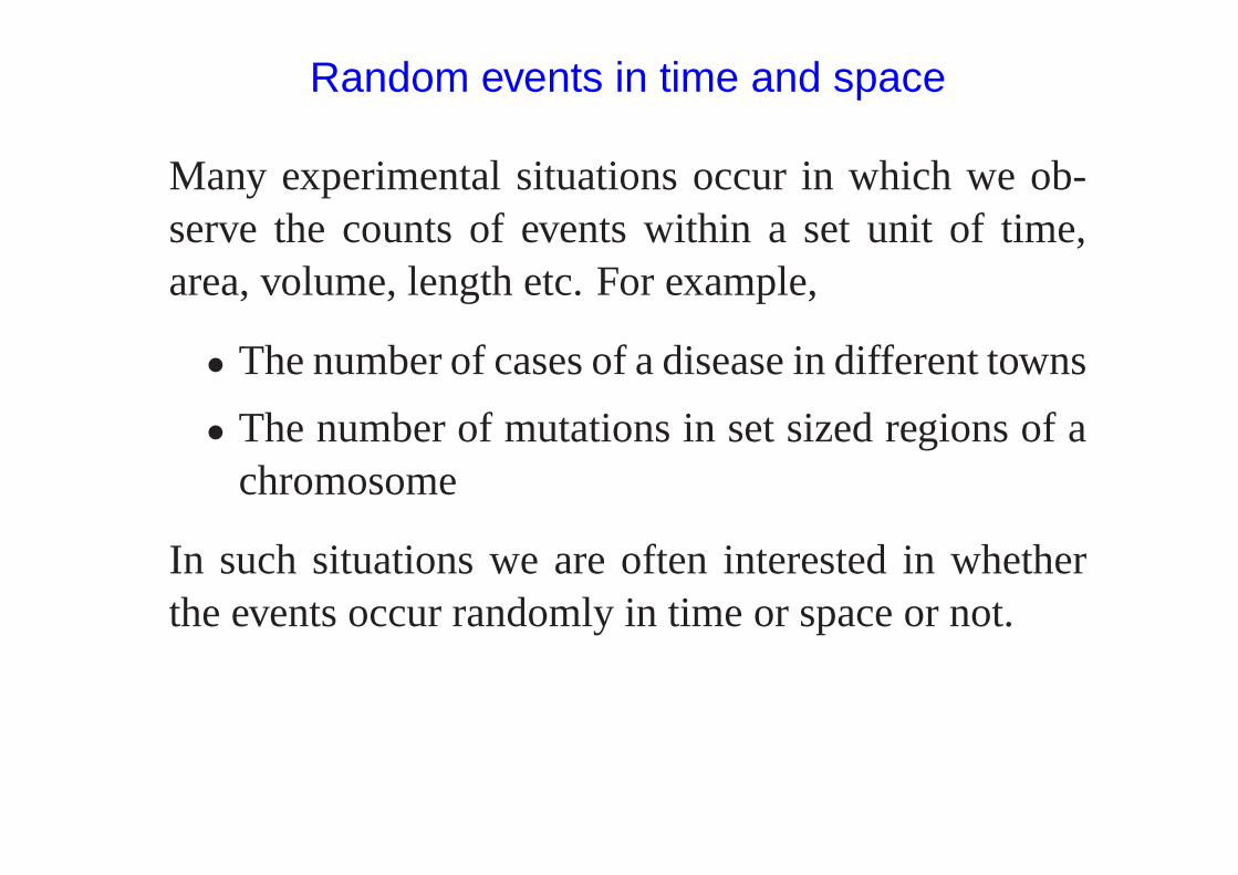
Consider the birth times from the Babyboom datasetwe saw in Lecture 2.
Birth Time (minutes since midnight)0 200 400 600 800 1000 1200 1440
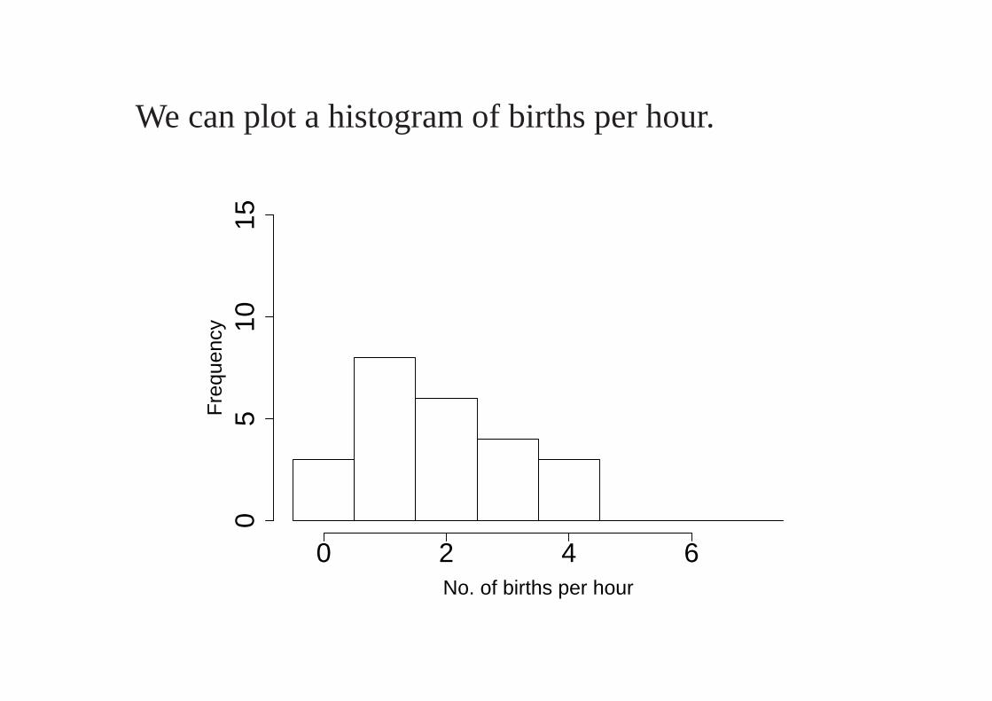
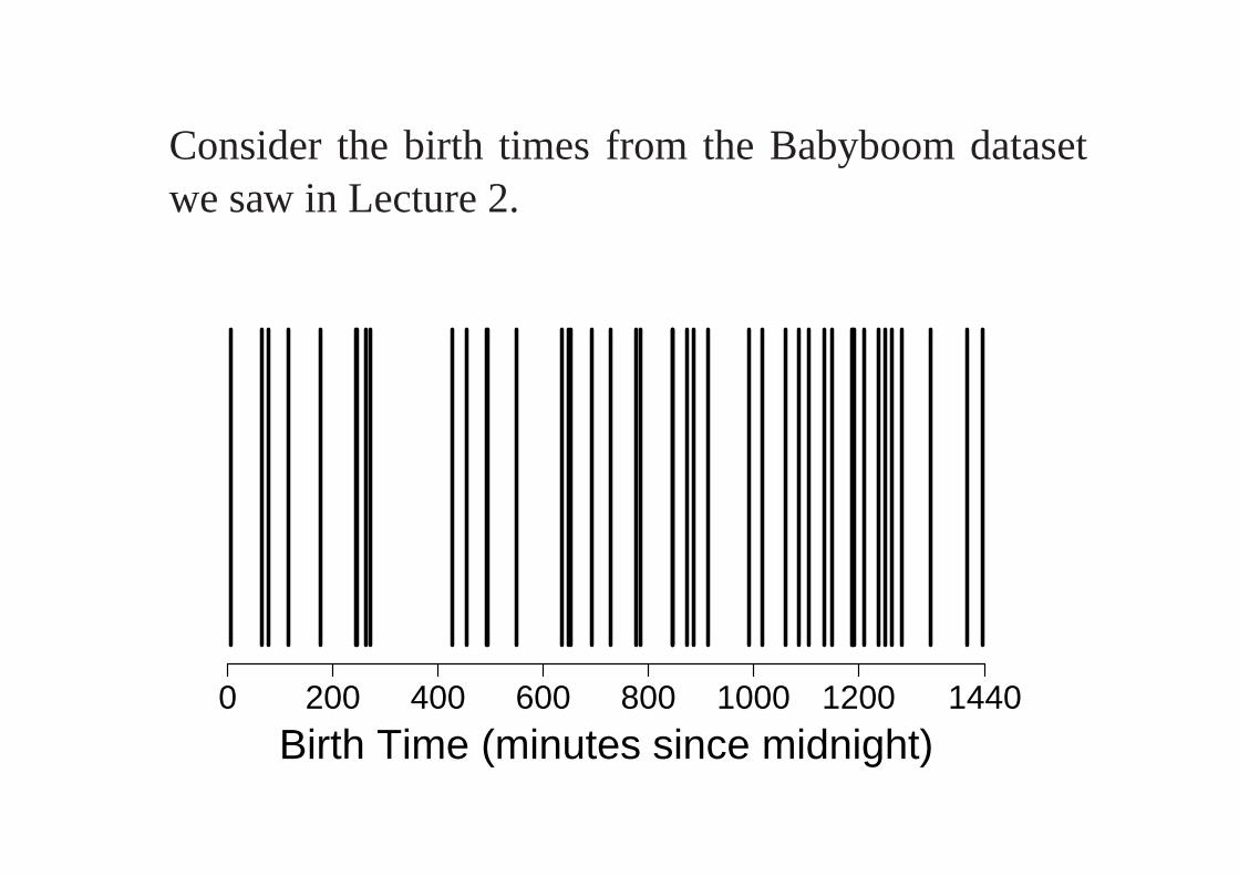
We can plot a histogram of births per hour.
No. of births per hour
Fre
quen
cy
0 2 4 6
05
1015
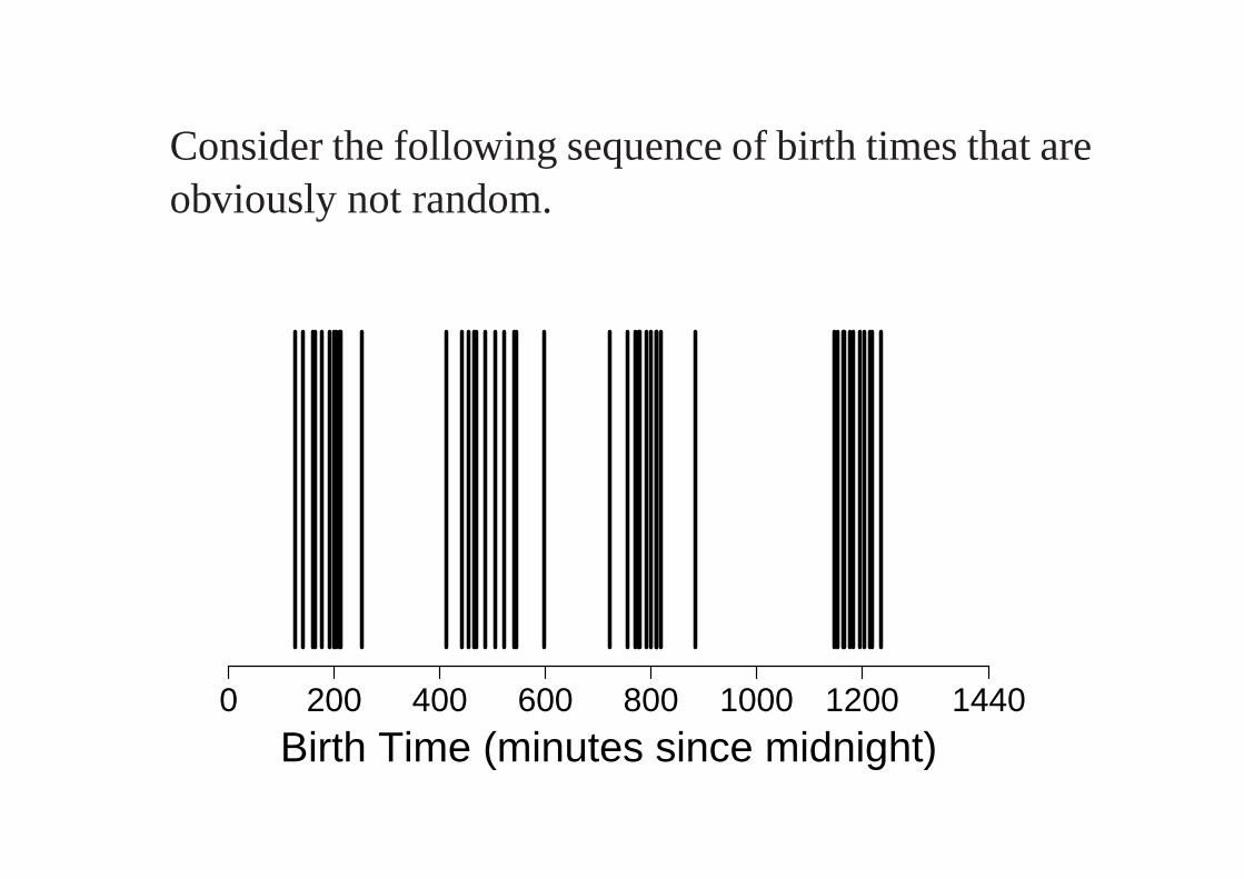
Consider the following sequence of birth times that areobviously not random.
Birth Time (minutes since midnight)0 200 400 600 800 1000 1200 1440
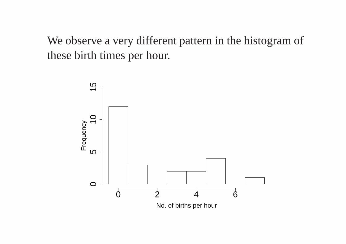
We observe a very different pattern in the histogram ofthese birth times per hour.
No. of births per hour
Fre
quen
cy
0 2 4 6
05
1015

This example illustrates that the distribution of countsis useful in uncovering whether the events might occurrandomly or non-randomly in time (or space).
Simply looking at the histogram isn’t sufficient if wewant to ask the question whether the events occurrandomly or not.
To answer this question we need a probability modelfor the distribution of counts of random events thatdictates the type of distributions we should expect tosee.
The Poisson Distribution
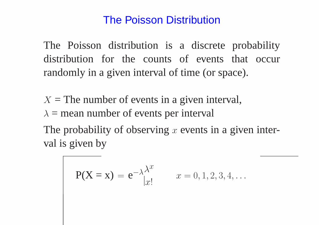
The Poisson distribution is a discrete probabilitydistribution for the counts of events that occurrandomly in a given interval of time (or space).
X = The number of events in a given interval,λ = mean number of events per interval
The probability of observingx events in a given inter-val is given by
P(X = x) = e−λλx
x!x = 0, 1, 2, 3, 4, . . .

Note e is a mathematical constant. e≈ 2.718282.There should be a button on your calculatorex thatcalculates powers of e.
If the probabilities of X are distributed in this way, wewrite
X∼Po(λ)
λ is the parameter of the distribution. Wesay Xfollows a Poisson distribution with parameterλ
Note A Poisson random variable can take on anypositive integer value. In contrast, the Binomialdistribution always has a finite upper limit.
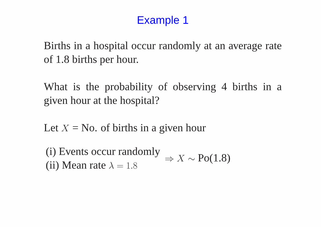
Example 1
Births in a hospital occur randomly at an average rateof 1.8 births per hour.
What is the probability of observing 4 births in agiven hour at the hospital?
Let X = No. of births in a given hour
(i) Events occur randomly(ii) Mean rateλ = 1.8
⇒ X ∼ Po(1.8)
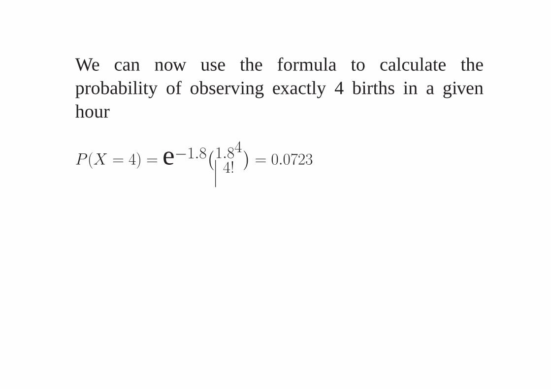
We can now use the formula to calculate theprobability of observing exactly 4 births in a givenhour
P (X = 4) = e−1.8(1.84
4!
)
= 0.0723
Example 2
What about the probability of observing more than orequal to 2 births in a given hour at the hospital?
We wantP (X ≥ 2) = P (X = 2) + P (X = 3) + . . .
i.e. an infinite number of probabilities to calculate
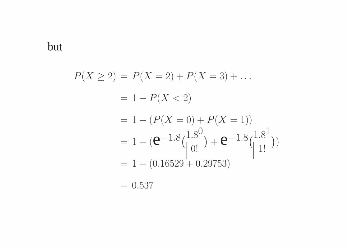
but
P (X ≥ 2) = P (X = 2) + P (X = 3) + . . .
= 1 − P (X < 2)
= 1 − (P (X = 0) + P (X = 1))
= 1 − (e−1.8(1.80
0!
)
+ e−1.8(1.81
1!
)
)
= 1 − (0.16529 + 0.29753)
= 0.537

Example 3
Jinkinson and Slater (1981) observed the nature ofqueues at a London Underground station. Theycounted the number of women present in queues oflength ten. The data for 100 such queues are presentedbelow:
No. women0 1 2 3 4 5 6 7 8 9 10Frequency 1 3 4 23 25 19 18 5 1 1 0
Which is model is appropriate for this data(a) Binomial, or (b) Poisson?
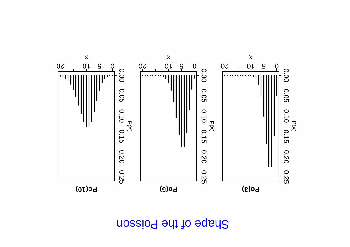
ShapeofthePoisson
051020
0.000.05
0.100.15
0.200.25
Po(3)
X
P(X
)
051020
0.000.05
0.100.15
0.200.25
Po(5)
X
P(X
)
051020
0.000.05
0.100.15
0.200.25
Po(10)
X
P(X
)

Poisson distributions are
(i) unimodal
(ii) exhibit positive skew (that decreases asλ in-creases)
(iii) centered roughly onλ
(iii) the variance (spread) increases asλ increases
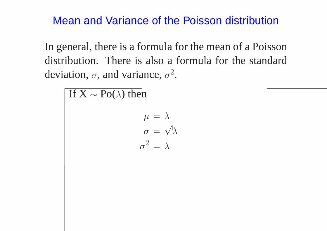
Mean and Variance of the Poisson distribution
In general, there is a formula for the mean of a Poissondistribution. There is also a formula for the standarddeviation,σ, and variance,σ2.
If X ∼ Po(λ) then
µ = λ
σ =√
λ
σ2 = λ
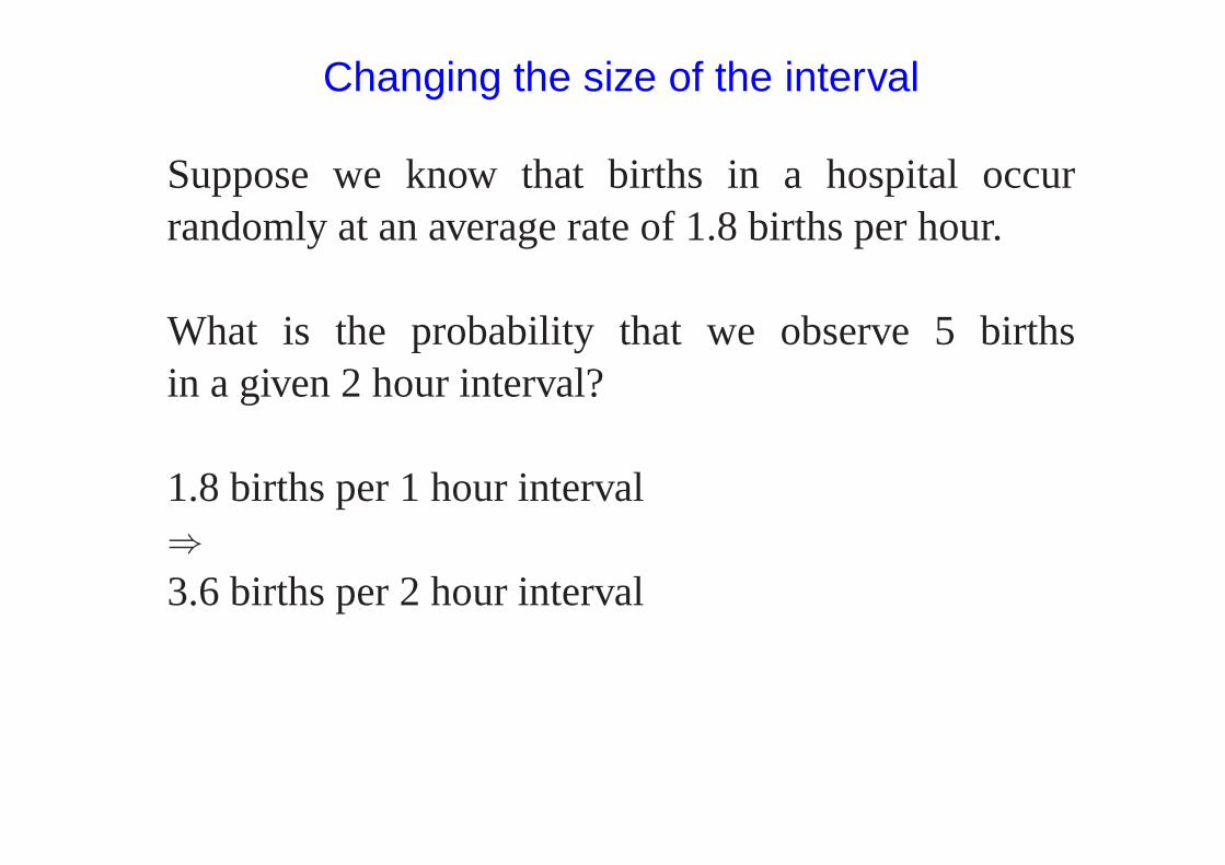
Changing the size of the interval
Suppose we know that births in a hospital occurrandomly at an average rate of 1.8 births per hour.
What is the probability that we observe 5 birthsin a given 2 hour interval?
1.8 births per 1 hour interval⇒3.6 births per 2 hour interval
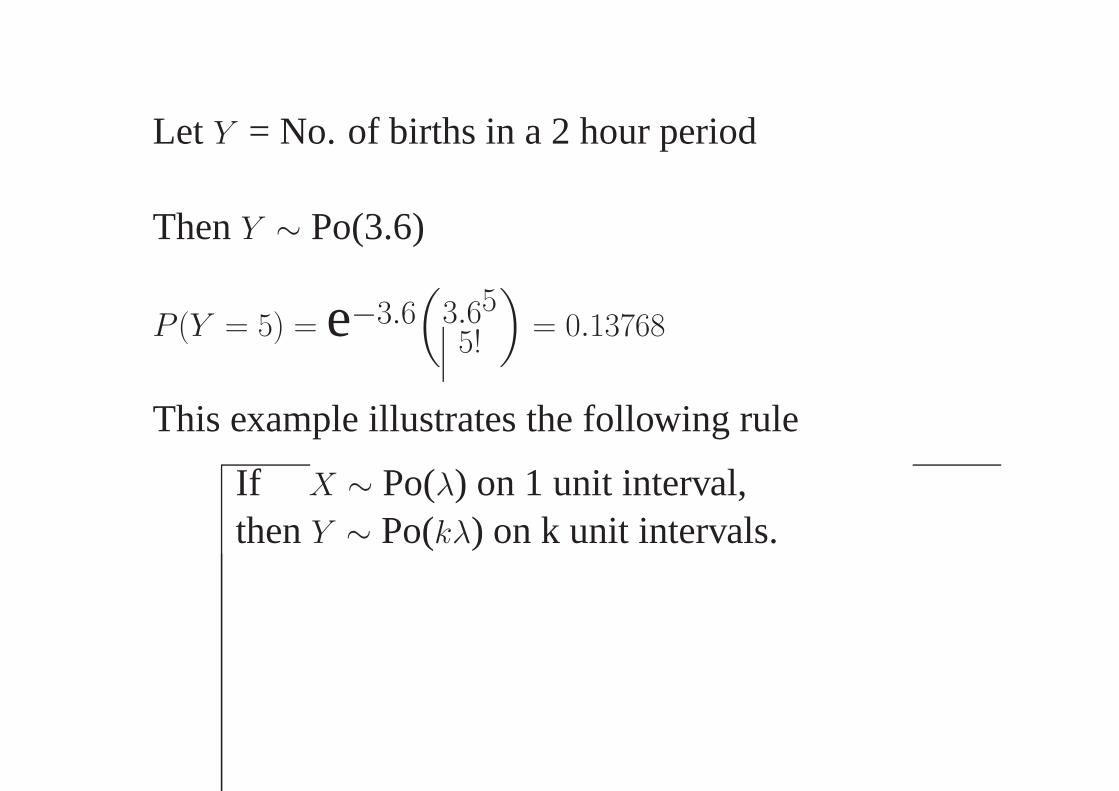
Let Y = No. of births in a 2 hour period
ThenY ∼ Po(3.6)
P (Y = 5) = e−3.6(
3.65
5!
)
= 0.13768
This example illustrates the following rule
If X ∼ Po(λ) on 1 unit interval,thenY ∼ Po(kλ) on k unit intervals.

Sum of two Poisson variables
Now suppose we know that in hospital A births occurrandomly at an average rate of 2.3 births per hour andin hospital B births occur randomly at an average rateof 3.1 births per hour.
What is the probability that we observe 7 birthsin total from the two hospitals in a given 1 hourperiod?
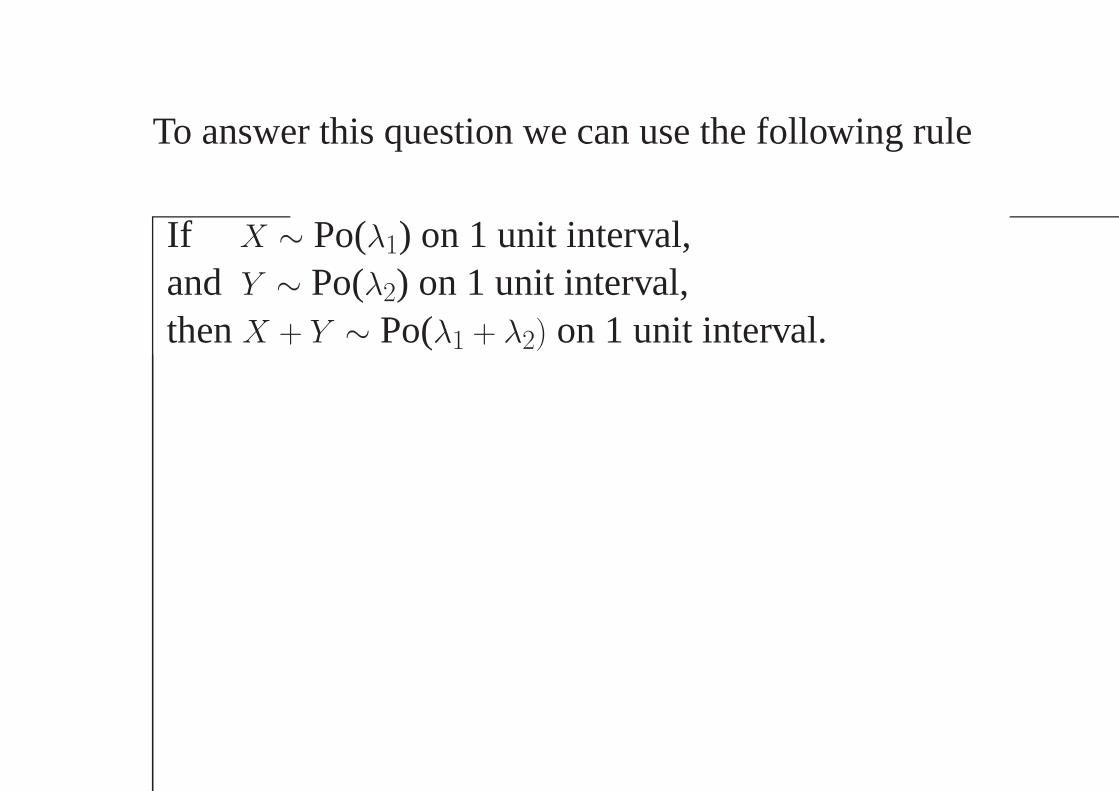
To answer this question we can use the following rule
If X ∼ Po(λ1) on 1 unit interval,and Y ∼ Po(λ2) on 1 unit interval,thenX + Y ∼ Po(λ1 + λ2) on 1 unit interval.
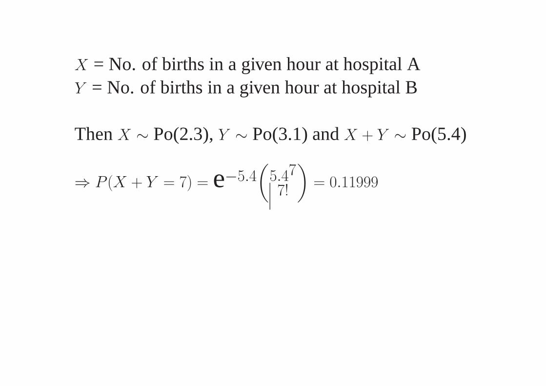
X = No. of births in a given hour at hospital AY = No. of births in a given hour at hospital B
ThenX ∼ Po(2.3),Y ∼ Po(3.1) andX + Y ∼ Po(5.4)
⇒ P (X + Y = 7) = e−5.4(
5.47
7!
)
= 0.11999
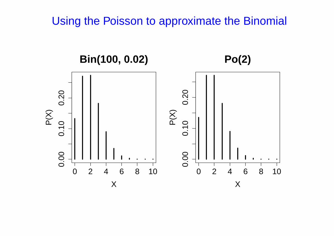
Using the Poisson to approximate the Binomial
0 2 4 6 8 10
0.00
0.10
0.20
Bin(100, 0.02)
X
P(X
)
0 2 4 6 8 10
0.00
0.10
0.20
Po(2)
X
P(X
)
In general,
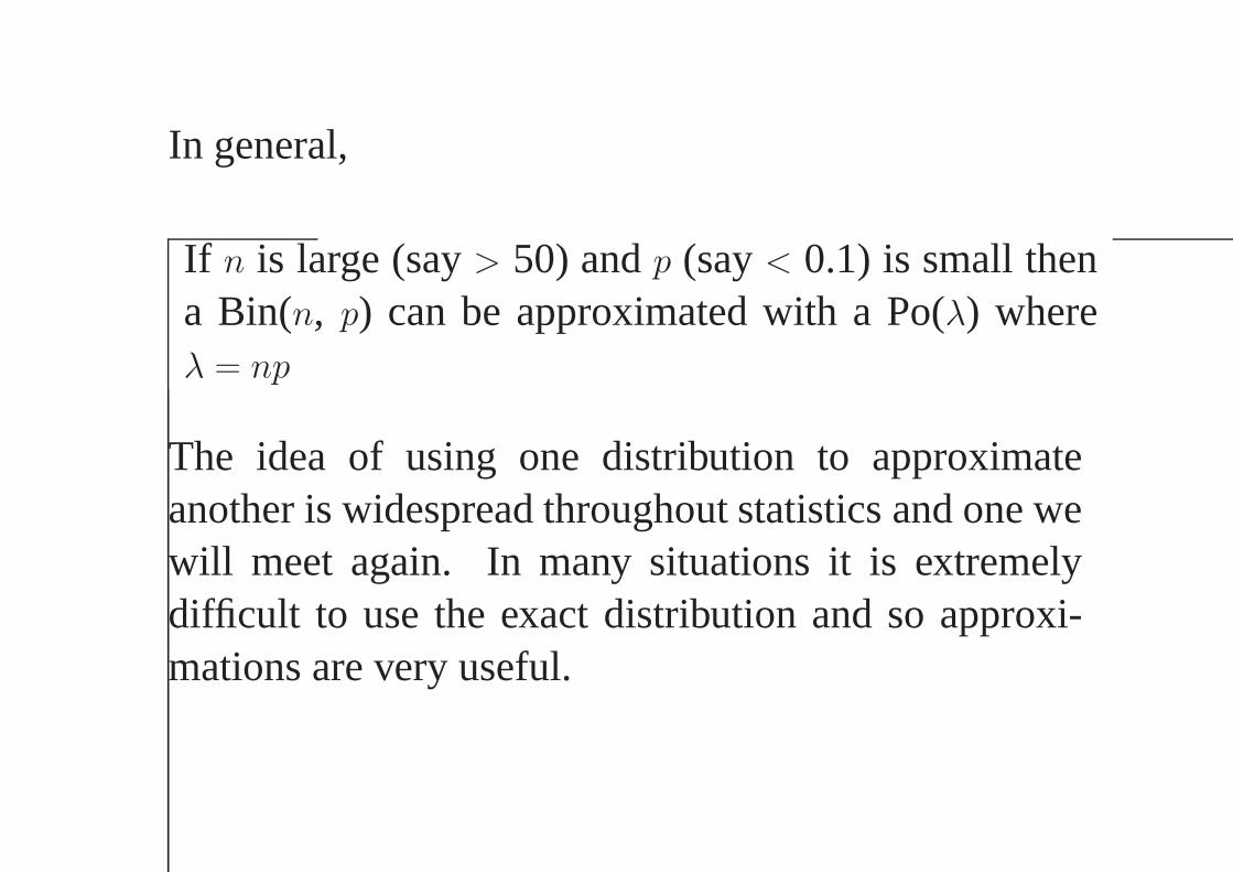
If n is large (say> 50) andp (say< 0.1) is small thena Bin(n, p) can be approximated with a Po(λ) whereλ = np
The idea of using one distribution to approximateanother is widespread throughout statistics and one wewill meet again. In many situations it is extremelydifficult to use the exact distribution and so approxi-mations are very useful.
Example
Given that5% of a population are left-handed, use thePoisson distribution to estimate the probability thata random sample of 100 people contains 2 or moreleft-handed people.
X = No. of left handed people out of 100
X ∼ Bin(100, 0.05)
Poisson approximation⇒ X ∼ Po(λ) with λ = 100 × 0.05 = 5
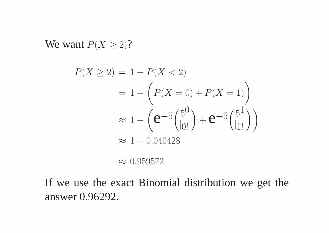
We wantP (X ≥ 2)?
P (X ≥ 2) = 1 − P (X < 2)
= 1 −(
P (X = 0) + P (X = 1)
)
≈ 1 −(
e−5(
50
0!
)
+ e−5(
51
1!
))
≈ 1 − 0.040428
≈ 0.959572
If we use the exact Binomial distribution we get theanswer 0.96292.
Fitting a Poisson distribution
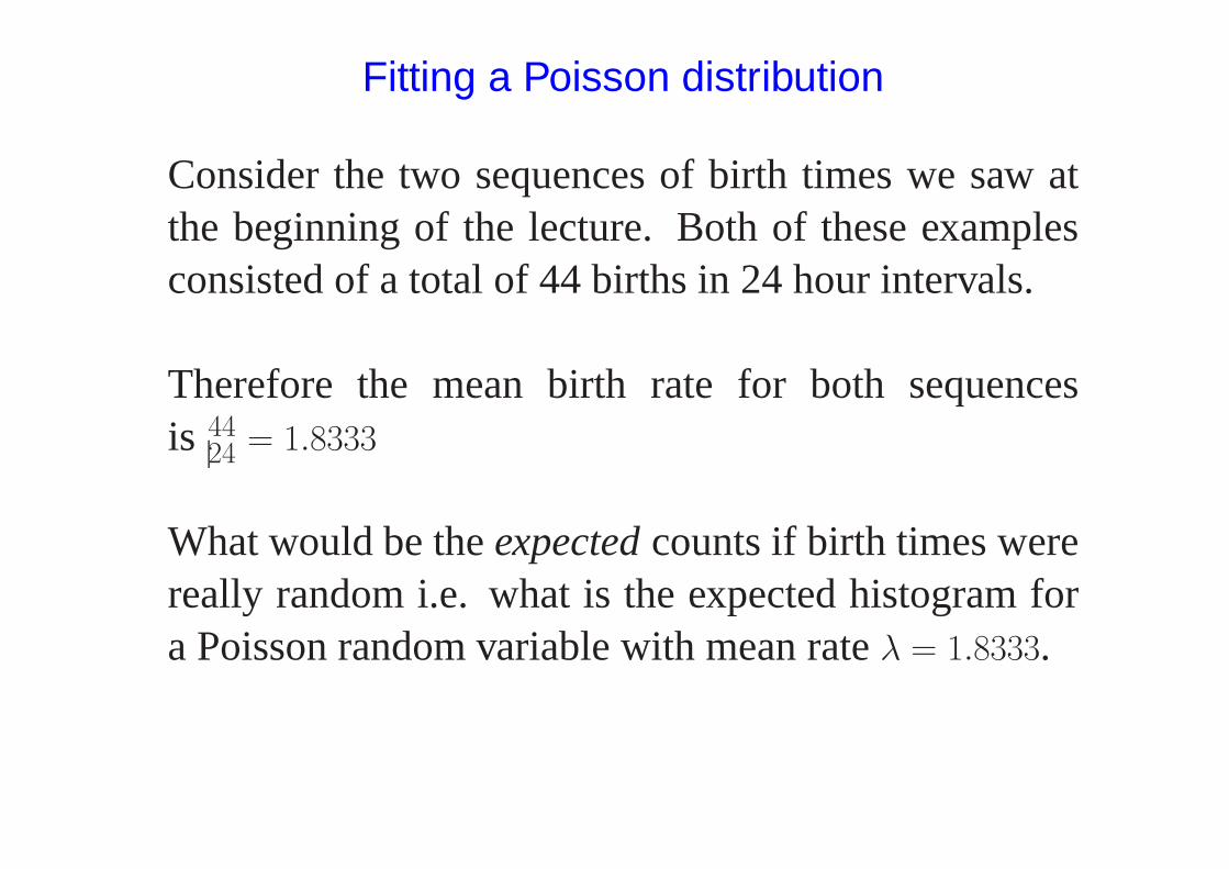
Consider the two sequences of birth times we saw atthe beginning of the lecture. Both of these examplesconsisted of a total of 44 births in 24 hour intervals.
Therefore the mean birth rate for both sequencesis 44
24 = 1.8333
What would be theexpected counts if birth times werereally random i.e. what is the expected histogram fora Poisson random variable with mean rateλ = 1.8333.
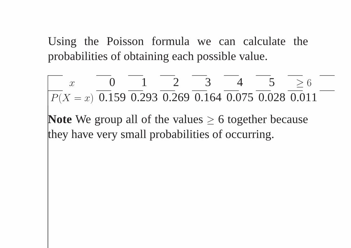
Using the Poisson formula we can calculate theprobabilities of obtaining each possible value.
x 0 1 2 3 4 5 ≥ 6
P (X = x) 0.159 0.293 0.269 0.164 0.075 0.028 0.011
Note We group all of the values≥ 6 together becausethey have very small probabilities of occurring.
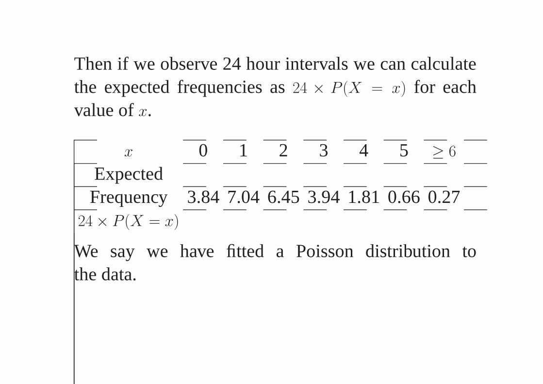
Then if we observe 24 hour intervals we can calculatethe expected frequencies as24 × P (X = x) for eachvalue ofx.
x 0 1 2 3 4 5 ≥ 6
ExpectedFrequency 3.84 7.04 6.45 3.94 1.81 0.66 0.27
24 × P (X = x)
We say we have fitted a Poisson distribution tothe data.

Fitting discrete distributions
3 steps
(i) Estimating the parameters of the distribution fromthe data
(ii) Calculating the probability distribution
(iii) Multiplying the probability distribution by thenumber of observations
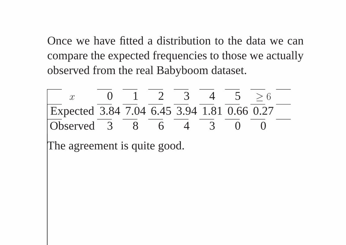
Once we have fitted a distribution to the data we cancompare the expected frequencies to those we actuallyobserved from the real Babyboom dataset.
x 0 1 2 3 4 5 ≥ 6
Expected3.84 7.04 6.45 3.94 1.81 0.66 0.27Observed 3 8 6 4 3 0 0
The agreement is quite good.
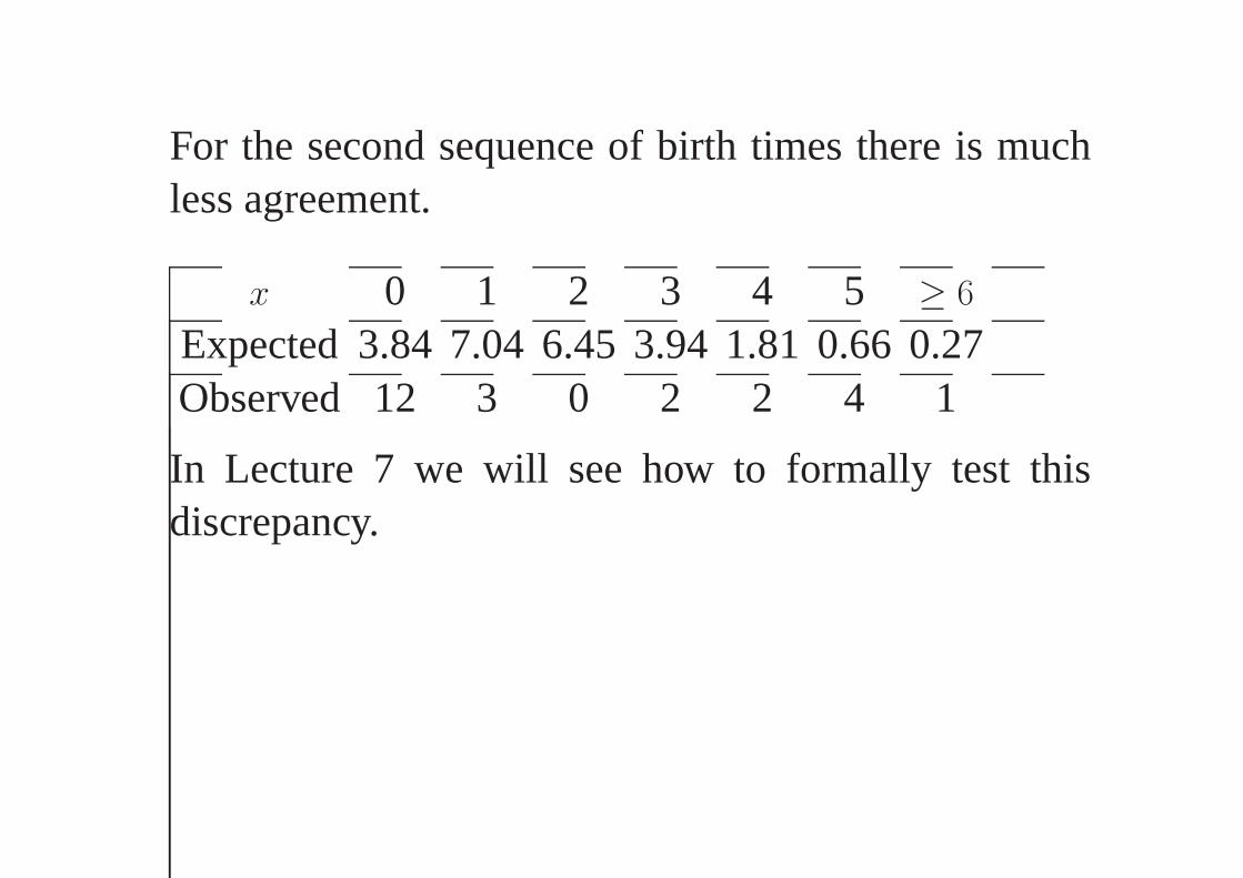
For the second sequence of birth times there is muchless agreement.
x 0 1 2 3 4 5 ≥ 6
Expected3.84 7.04 6.45 3.94 1.81 0.66 0.27Observed 12 3 0 2 2 4 1
In Lecture 7 we will see how to formally test thisdiscrepancy.